235
LECTURE NOTES IN ANALYSIS (2011) Sergiu Klainerman Department of Mathematics, Princeton University, Princeton NJ 08544 E-mail address : [email protected]
| Date post: | 06-Feb-2018 |
| Category: |
Documents |
| Upload: | nguyennguyet |
| View: | 215 times |
| Download: | 0 times |
LECTURE NOTES IN ANALYSIS (2011)
Sergiu Klainerman
Department of Mathematics, Princeton University, Princeton NJ 08544
E-mail address: [email protected]


Part 1
INTRODUCTION TO PDE
1. The world of PDE
To start with partial differential equations, just like ordinary differential or integralequations, are functional equations. That means that the unknown, or unknowns,we are trying to determine are functions. In the case of partial differential equa-tions (PDE) these functions are to be determined from equations which involve, inaddition to the usual operations of addition and multiplication, partial derivativesof the functions. Below are the most basic examples,
• (Laplace equation)
∆u = 0 (1)
where ∆u = ∂2
∂x2u+ ∂2
∂y2u+ ∂2
∂z2u. The other two examples described in the section
of fundamental mathematical definitions are
• (Heat Equation)
− ∂tu+ k∆u = 0, (2)
• (Wave equation)
− ∂2t u+ c2∆u = 0. (3)
In both cases one is asked to find a function u, depending on the variables t, x, y, z,which verifies the corresponding equations. Observe that both (2) and (3) in-volve the symbol ∆ which has the same meaning as in the first equation, that is
∆u = ( ∂2
∂x2 + ∂2
∂y2 + ∂2
∂z2 )u = ∂2
∂x2u + ∂2
∂y2u + ∂2
∂z2u. In both (2) and (3) k > 0 and
c are fixed constants (representing the rate of diffusion for the first and the speedof light in the second). It suffices to study to solve the equations for the specialcases k = 1 and c = 1. Indeed if u(t, x, y, z) is a solution of (3), for example, thenv(t, x, y, z) = u(t, x/c, y/c, z/c) verifies the same equation with c = 1. Both equa-tions are called evolution equations, simply because they are supposed to describethe change relative to the time parameter t of a particular physical object. Observethat (1) can be interpreted as a particular case of both (3) and (2). Indeed solutionsu = u(t, x, y, z) of either (3) or (2) which are independent of t, i.e. ∂tu = 0, verify(1).
Here are some further examples of important PDEs:
• (Schrodinger equation)
i∂tu+ k∆u = 0 (4)
with u : R× R3 → C. The equation describes the quantum evolution of a massiveparticle, k = ~
2m , where ~ > 0 is Planck’s constant and m is the mass of theparticle. As with the heat equation, one can normalize k = 1 by a simple change ofvariables. Though the equation is formally very similar to the heat equation, it hasvery different qualitative behavior. It is important to keep in mind when studying
1. THE WORLD OF PDE 5
PDE’s that small changes in the form of an equation can lead to very differentproperties of solutions.
• (Klein-Gordon equation)
− ∂2t u+ c2∆u−
(mc2
~
)2
u = 0 (5)
This is the relativistic counterpart to the Schrodinger equation, the parameter mhas the physical interpretation of mass and mc2 has the physical interpretation ofrest energy (reflecting Einstein’s famous equation E = mc2). One can normalize
the constants c and mc2
~ to make them both equal 1 by applying a suitable changeof variables to both time and space.
Observe that all three PDE mentioned above satisfy the following simple propertycalled the principle of superposition: If u1, u2 are solutions of an equation so isany linear combination of them λ1u1 + λ2u2 where λ1 and λ2 are arbitrary realnumbers. Such equations are called linear. The following equation in the unknownu = u(x, y), is manifestly not linear:
• (Minimal surfaces
∂x( ∂xu
(1 + |∂xu|2 + |∂yu|2)12
)+ ∂y
( ∂yu
(1 + |∂xu|2 + |∂yu|2)12
)= 0. (6)
Here ∂x and ∂y are short hand notations for the partial derivatives ∂∂x and ∂
∂y .
The equations we have encountered so far can be written in the form P[u] = 0,where P is a differential operator applied to u. A differential operator is simply arule which takes functions u, defined in Rn or an open subset of it, into functionsP[u] by performing the following operations:
• We can take partial derivatives ∂iu = ∂u∂xi relative to the variables x =
(x1, x2, . . . xn) of Rn. One allows also higher partial derivatives of u such
as the mixed second partials ∂i∂ju = ∂2u∂xi∂xj or ∂2
i = ∂2
∂x2i.
The associated differential operators for (2) is P = −∂t + ∆ and thatof (3) is −∂2
t + ƥ Can add and multiply u and its partial derivatives between themselves as
well as with given functions of the variables x. Composition with givenfunctions may also appear.
In the case of the equation (1) the associated differential operator is P = ∆ =
∂21 + ∂2
2 + ∂23 =
∑3i,j=1 e
ij∂i∂j where eij is the diagonal 3 × 3 matrix with entries
(1, 1, 1) corresponding to the euclidean scalar product of vectors X,Y in R3,
< X,Y >= X1Y1 +X2Y2 +X3Y3 =
3∑i,j=1
eijXiXj . (7)
6
The associated differential operators for (2), (3) and (4) are, resp. P = −∂t + ∆,P = −∂2
t + ∆ and P = i∂t + ∆ with variables are t, x1, x2, x3 ∈ R1+3. In theparticular case of the wave equation (3) it pays to denote the variable t by x0. Thewave operator can then be written in the form,
= −∂20 + ∂2
1 + ∂22 + ∂2
3 =
3∑α,β=0
mαβ∂α∂β (8)
where mαβ is the diagonal 4× 4 matrix with entries (−1, 1, 1, 1), corresponding tothe Minkowski scalar product in R1+3. This latter scalar product is defined, for 4vectors X = (X0, X1, X2, X3) and Y = (Y0, Y1, Y2, Y3) by,
m(X,Y ) =
3∑α,β=0
mαβXαYβ = −X0Y0 +X1Y1 +X2Y2 +X4Y4 (9)
The differential operator is called D’Alembertian after the name of the Frenchmathematician who has first introduced it in connection to the equation of a vi-brating string.
Observe that the differential operators associated to the equations (1)–(4) are alllinear i.e.
P[λu+ µv] = λP[u] + µP[v],
for any functions u, v and real, or complex, numbers λ, µ. The following is anothersimple example of a linear differential operator
P[u] = a1(x)∂1u+ a2(x)∂2u (10)
where x = (x1, x2) and a1, a2 are given functions of x. They are called the coeffi-cients of the linear operator. An equation of the form
P[u] = f, (11)
corresponding to a linear differential operator P and a given function f = f(x), iscalled linear-inhomogeneous . Any solution u of such an equation can be expressedin the form u = u0 + v where u0 is a special solution of (11) and v solution to thehomogeneous equation
P[v] = 0. (12)
In the case of the equation (6) the differential operator P can be written, relativeto the variables x1 and x2, in the form,
P[u] =
2∑i=1
∂i
(1
(1 + |∂u|2)12
∂iu
),
where |∂u|2 = (∂1u)2 + (∂2u)2. Clearly P[u] is not linear in this case. We callit a nonlinear operator; the corresponding equation (6) is said to be a nonlinearequation. An important property of both linear and nonlinear differential operatorsis locality. This means that whenever we apply P to a function u, which vanishesin some open set D, the resulting function P[u] also vanish in D.
Observe also that our equations (1)-(4) are also translation invariant. This means,in the case (1) for example, that whenever the function u = u(x) is a solution so
1. THE WORLD OF PDE 7
is the function uc(x) := u(Tcx) where Tc is the translation Tc(x) = x + c. Onthe other hand the equation P[u] = 0, corresponding to the operator P defined by(10) is not, unless the coefficients a1, a2 are constant. Clearly the set of invertibletransformations1 T : Rn → Rn which map any solution u = u(x), of P[u] = 0, toanother solution uT (x) := u(Tx) form a group, called the invariance group of theequation. The composition of two symmetries is again a symmetry, as is the inverseof a symmetry, and so it is natural to view a collection of symmetries as forming agroup (which is typically a finite or infinite-dimensional Lie group).
The Laplace equation (1) is invariant not only with respect to translations but alsorotations, i.e linear transformations O : R3 → R3 which preserve the euclideanscalar product (7) in the sense that < OX,OY >=< X,Y > for all vectors X,Y ∈R3. Similarly the wave equation (3) and Klein-Gordon equation (5) are invariantunder Lorentz transformations, i.e. linear transformations L : R1+3 → R1+3 whichpreserve the Minkowski scalar product (9), i.e. m(LX,LY ) = m(X,Y ). Ourother evolution equations (2) and (4) are clearly invariant under rotations of thespace variables x = (x1, x2, x3) ∈ R3, keeping t fixed. They are also Galileaninvariant, which means, in the particular case of the Schrodinger equation (278),
that whenever u = u(t, x) is a solution so is uv(t, x) = ei(x·v)eit|v|2
u(t, x − vt) forany vector v ∈ R3.
So far we have tacitly assumed that our equations take place in the whole space –R3 for the Laplace equation, R4 for the Heat, Wave and Schrodinger equations andR2 for the minimal surface equation. In reality, one is often restricted to a domainof the corresponding space. Thus, for example, the equation (1) is usually studiedon a bounded open domain of R3 subject to a specified boundary condition. Hereis a typical example.
Example. The Dirichlet problem on an open domain of D ⊂ R3 consists offinding a continuous functions u defined on the closure D of D, twice continuouslydifferentiable in D, such that ∆u = 0 in D and the restriction of u to ∂D, theboundary of D, is prescribed to be a continuous function u0. More precisely werequire that,
u|∂D = u0 (13)
One can impose the same boundary condition for solutions of (6), with D a boundedopen domain of R2. A solution u = u(x, y) of (6) in D, verifying the boundarycondition (13), solves the Plateau problem of finding minimal surfaces in R3 whichpass through a given curve. One can show that the surface given by the graphΓu = (x, y, u(x, y))/(x, y) ∈ D ⊂ R2 has minimum area among all other graphsurfaces Γv verifying the same boundary condition, v|∂D = u0.
Natural boundary conditions can also be imposed for the evolution equations (2)–(4). The simplest one is to prescribe the values of u on the hyperplane t = 0. Inthe case of the heat and Schrodinger equation we set,
u|t=0 = u0
1The transformations are often linear maps.
8
while in the case of the wave equation, which involves a second derivative in t, weimpose two conditions
u|t=0 = u0 and ∂tu|t=0 = u1 (14)
where u0, u1 are functions of the coordinates (x, y, z), called initial conditions. Tosolve the initial value problem in both cases means to find solutions of the equationsfor t > 0 which verify the corresponding initial conditions at t = 0. In additionone may restrict the variables (x, y, z) to an open domain of D ⊂ R3. More to thepoint one may try to solve a boundary value problem in a domain [0,∞)×D with aboundary condition, such as (13), on [0,∞)× ∂D and an initial condition at t = 0.
The choice of boundary condition and initial conditions, for a given PDE, is veryimportant. Finding which are the good boundary and initial conditions is an im-portant aspect of the general theory of PDE which we shall address in section 2.For equations of physical interest these appear naturally from the context in whichthey are derived. For example, in the case of a vibrating string, which is describedby solutions of the one dimensional wave equation ∂2
t u − ∂2xu = 0 in the domain
(a, b) × R, the initial conditions u = u0, ∂tu = u1 at t = t0, amount to specifyingthe original position and velocity of the string. On the other hand the boundarycondition u(a) = u(b) = 0 simply mean that the two ends of the of the string arefixed.
So far we have only considered equations in one unknown. In reality many ofthe equations of interest appear as systems of partial differential equations. Thefollowing important example, contains two unknown functions u1 = u1(x1, x2), u2 =u2(x1, x2) which verify,
• (Cauchy-Riemann)
∂1u2 − ∂2u1 = 0, ∂1u1 + ∂2u2 = 0 (15)
It was first observed by Cauchy that u = u1 + iu2, as a function of z = x1 + ix2, is acomplex analytic function if and only if (15) is satisfied. Setting also ∂ = ∂1 + i∂2,observe that (15) is equivalent to
∂u = 0. (16)
Equation (15) can also be written in the form P[u] = 0 by introducing u = (u1, u2)as a column vector and P[u] the differential operator,
P[u] =
(−∂2 ∂1
∂1 ∂2
)·(u1
u2
)The system of equations (15) contains two equations and two unknowns. This isthe standard situation of a determined system. A system is called over-determinedif it contains more equations than unknowns and underdetermined if it containsfewer equations than unknowns. For example the system of two equations andone unknown ∂xu(x, y) = f, ∂yu(x, y) = g is clearly overdetermined. A necessarycondition for a solution to exist is ∂yf = ∂xg, condition which can be interpreted
1. THE WORLD OF PDE 9
as requiring that the one-form w = f(x, y)dx + g(x, y)dy is exact, i.e. its exte-rior derivative dω is identically zero. Overdetermined systems, such as De Rhamcomplexes, play a very important role in geometry.
Observe that (15) is a linear system. Observe also that the operator P has thefollowing remarkable property.
P2[u] = P[P[u]] =
(∆u1
∆u2
)In other words P2 = ∆ · I, with I the identity operator I[u] = u, and thereforeP can be viewed as a a square root of ∆. One can define a similar type of squareroot for the D’Alembertian . To achieve this we need 4 × 4 complex matricesγ0, γ1, γ3, γ4 which satisfy the property
γαγβ + γβγα = −2mαβI (17)
with I the unit 4 × 4 matrix and mαβ as in (8). Using the γ matrices we canintroduce the Dirac operator acting on u = (u1, u2, u3, u4) defined from R1+3 withvalues in C4 by,
Du = iγα∂αu (18)
Using (17) we easily check that, D2u = u. Thus the Dirac operator D can beviewed as a square root of the D’Alembertian . It leads to the following funda-mental equation introduced by Dirac as the equation of free, massive, relativistic,particle such as the electron:
• (Dirac Equation)
Du = ku (19)
Partial differential equations are ubiquitous throughout Mathematics and Science.They provide the basic mathematical framework for some of the most importantphysical theories, such as Elasticity, Hydrodynamics, Electromagnetism, GeneralRelativity and Non-relativistic Quantum Mechanics. The more modern relativisticquantum field theories lead, in principle, to equations in infinite number of un-knowns, which lie beyond the scope of partial differential equations. Yet, even inthat case, the basic equations preserve the locality property of PDE. Moreover thestarting point of a quantum field theory is always a classical field theory, describedby systems of PDE’s. This is the case, for example, of the Standard Model of weakand strong interactions, based on a Yang -Mills-Higgs field theory. If we also includethe ordinary differential equations of Classical Mechanics, which can be viewed asone dimensional PDE, we see that, essentially, all of Physics is described by differ-ential equations. Other examples of partial differential equations underlining someof our most basic physical theories, are the Maxwell, Einstein, Euler and NavierStokes equations. Note that each equation are at the heart of an entire field ofPhysics, i.e. Electrodynamics, General Relativity and Hydrodynamics,
An important feature of the main PDEs appearing in Physics is their apparentuniversality. Thus, for example, the wave equation, first introduced by D’alembertto describe the motion of a vibrating string was later found to be connected tothe propagation of sound and electromagnetic waves. The heat equation, first
10
introduced by Fourier to describe heat propagation, also comes in many othersituations in which dissipative effects play an important role. The same thing canbe said about the Laplace, Schrodinger and many other basic equations.
It is even more surprising that equations, originally introduced to describe specificphysical phenomena, also play a fundamental role in areas of mathematics, whichare considered pure, such as Complex Analysis, Differential Geometry, Topologyand Algebraic Geometry. Complex Analysis, for example, which studies the prop-erties of holomorphic functions, can be regarded as the study of solutions to theCauchy-Riemann equations (15) in a domain of R2. Hodge theory, which playsa fundamental role in topology and algebraic geometry, is based on studying thespace of solutions to a class of linear systems of partial differential equations onmanifolds which generalize the Cauchy-Riemann equations. The Atiyah-Singer in-dex theorem is formulated in terms of a special classes of linear PDE on manifolds,related to the euclidean version of the Dirac operator (18).2
Important problems in geometry can be reduced to finding solutions to specificpartial differential equations, typically nonlinear. We have already seen such anexample in the case of the Plateau problem of finding surfaces of minimal totalarea which pass through a given curve. The well known uniformization theoremprovides another excellent example.
To state the uniformization theorem, we need to recall the definition of a compactRiemann surface S. This is a 2 -dimensional, compact manifold endowed with asmooth, positive definite metric g. The Gauss curvature K = K(g) is an importantinvariant of the surface which can be calculated explicitely at every point p ∈S in terms of the components gab relative to a local system of coordinates x =(x1, x2) near p. The calculation involves first and second partial derivatives of thecomponents gab relative to x1 and x2. The remarkable fact is that the final value ofK does not depend on the particular system of coordinates in which one makes thecalculation. Moreover in the particular case when S is the standard sphere in R3,given by the equation |x|2 = a2, the Gauss curvature is equal to the expected value,corresponding to our intuition of curvature, that is K = a−2. Another remarkableproperty of the Gauss curvature is that its total integral along S does not depend onthe metric g but only on the topological properties of S. More precisely, accordingto the Gauss-Bonnet formula, we have
χ(S) = (2π)−1
∫S
Kdag,
with dag denoting the area element of the metric g. In coordinates x1, x2 we have
dag =√|g|dx1dx2 with |g| the determinant of the matrix (gab)a,b=1,2. The number
χ(S) is one of the integers 2, 0,−2, . . . − 2k . . . , called the Euler characteristic ofS, and has simple topological interpretation. Thus any surface which can be con-tinuously deformed to the standard sphere has χ(S) = 2 while any surface whichcan be continuously deformed to a torus has χ(S) = 0. We can now state theuniformization theorem:
2This is the operator obtained when we change the minkowski metric m to the euclidean onee in (17).
1. THE WORLD OF PDE 11
Theorem 1.1. Let S be a 2-dimensional, compact, Riemann surface with metric g,Gauss curvature K = K(g) and Euler characteristic χ(S). There exists a conformaltransformation of the metric g, i.e. g = Ω2g, for some smooth non-vanishingfunction Ω, such that the Gauss curvature K of the new metric g is identical equalto 1, 0 or −1 according to whether χ(S) > 0, χ(S) = 0 or χ(S) < 0.
To prove this very important geometric result, which leads to the complete classi-fication of all compact surfaces according to their Euler characteristic, we are ledto a nonlinear partial differential equation on S. Indeed assume that χ(S) = 2 and
therefore we want the Gauss curvature K of the metric g = e2ug to be exactly 1.It is easy to relate K, by a simple calculation, to the Gauss curvature K of theoriginal metric g . This leads to the following equation in u,
∆Su+ e2u = K (20)
where ∆S , called the Laplace-Beltrami operator of S, is a straightforward adap-tation of the Laplace operator, see (1), to the surface S. Thus the proof of theuniformization theorem reduces to solve equation (20), i.e. for a given surface Swith Gauss curvature K, find a real valued function u which verifies (20).
We give below a precise definition of the operator ∆S relative to a system of lo-cal coordinates x = (x1, x2) on an open coordinate chart D ⊂ S. Denote byG(x) = (gab(x))a,b=1,2 the 2 × 2 matrix whose entries are the components of ourRiemannian metric on D. Let G−1(x) denote the matrix inverse to G(x) and denoteits components by (gab(x))a,b=1,2. Thus, for all x ∈ D,∑
c
gac(x)gcb(x) = δab
with δab the usual Kronecker symbol. We also set, as before, |g(x)| = det(G(x))and define,
∆Su(x) =1√|g(x)|
∑a,b=1,2
∂b(√|g(x)| gab(x) ∂au(x))
Typically we suppress the explicit dependence on x in the above formula. It is alsovery convenient to use Einstein’s summation convention over repeated indices, andthus write,
∆Su =1√|g|∂b(√|g| gab ∂au) (21)
As a third example we consider the Ricci flow equation on a compact n dimen-sional manifold M , which is described in one of the articles of the Compendium. Inthe particular case of three dimensions the equation has been recently used, deci-sively, to provide the first proof of Thurston’s geometrization conjecture, includingthe well known Poincare conjecture. The geometrization conjecture, described inthe topology section of the Compendium, is the precise analogous, in three spacedimensions, of the 2-dimensional uniformization theorem mentioned above. TheRicci flow is defined, in arbitrary local coordinates x = (x1, x2, x3) on M , by theequation:
12
• (Ricci Flow)
∂tgij = Rij(g) (22)
Here gij = gij(t) is a family of Riemannian metrics depending smoothly on theparameter t and Rij(g) denotes the Ricci curvature of the metric gij . This is simplya three dimensional generalization of the Gauss curvature we have encounteredin the uniformization theorem. In a given system of coordinates Rij(g) can becalculated in terms of the metric coefficients gij and their first and second partialderivatives. Since both gij and Rij are symmetric relative to i, j = 1, 2, 3 we caninterpret (22) as a non-linear system of six equations with six unknowns. On acloser look it turns out that (22) is related to the heat equation (2). Indeed, bya straightforward calculation relative to a particular system of coordinates x =(x1, x2, x2) called harmonic, it can be shown that the Ricci flow (22) takes the form
∂tgij −∆ggij = Nij(g, ∂g) (23)
where each Nij , i, j = 1, 2, 3, are functions of the components gij and their firstpartial derivatives with respect to the coordinates x and ∆g is, again, a differentialoperator very similar to the Laplacian ∆ in R3, see (??). More precisely, if G−1 =(gab)a,b=1,2,3 denotes the matrix inverse to G = (gab)a,b=1,2,3 we can write, usingthe summation convention,
∆g = gab∂a∂b =
3∑a,b=1
gab∂a∂b.
In a small neighborhood of a point p ∈M we can choose the harmonic coordinatexa such that gab(p) = δab with δab denoting the usual Kronecker symbol. Thus,near p, ∆g looks indeed like ∆ = δab∂a∂b.
The Ricci flow3 allows one to deform an arbitrary Riemannian metric on M to a asimple metric of constant sectional curvature. The idea is to start with a metric gand look for solutions g(t) of (22) which verify the initial condition g(0) = g. Onehopes that as t→∞ the metric g(t) will converge to a metric of constant curvature.Intuitively one can see this working out the same way heat gets evenly distributedin space, as t increases, according to the heat equation (2). Indeed since (22) issimilar to (2) we expect the variations in the curvature of g(t) to become smallerand smaller as the metric evolves according to (22). The type of metric we get inthe limit as t→∞ will allow us to determine the topological character of M . Theflow, however, can develop singularities before we achieve that goal. To overcomethis major technical difficulty one needs to make a detailed qualitative analysis ofthe behavior of solutions to (22), task which requires just about all the advancesmade in geometric PDE in the last hundred years.
As we have seen above the choice of harmonic coordinates allows us to write theRicci flow as a system of nonlinear heat equations (23). This fact is quite typicalto geometric equations. It is useful at this point to discuss another importantexample, that of the Einstein equations in vacuum. An introduction to this equation
3In reality one needs to change the equation (22) slightly to make sure that the total volumeof of M , calculated with respect to the metric g(t), stays constant.
1. THE WORLD OF PDE 13
and short discussion of its importance in General Relativity can be found (seecompendium article). Solutions to the Einstein vacuum equations are given byRicci flat spacetimes, that is Lorentzian manifolds (M, g) with M a four dimensionalmanifold and g a Lorentz metric on it, for which the corresponding Ricci curvaturevanishes identically.
• (Einstein-vacuum)
Ric(g) = 0. (24)
The Ricci curvature of a Lorentz metric, Ric(g), can be defined in exactly the sameway as in the Riemannian case. Thus relative to a coordinate system xα, withα = 0, 1, 2, 3, the Ricci curvature, denoted by Rαβ , can be expressed in terms ofthe first and second partial derivatives of the metric coefficients gαβ . As before,we denote by gαβ the components of the inverse metric. Moreover, by pickinga specified system of coordinates, called wave coordinates4, we can express theEinstein-vacuum equations (24) in the form of a system of equations related to thewave equation (3), in the same way the Ricci flow system (23) was related to theheat equation (2). More precisely,
g gαβ = Nαβ(g, ∂g) (25)
where, as in the case of the Ricci flow, the terms Nαβ(g, ∂g) are expressions, whichcan be calculated explicitely, depending on the metric gαβ , its inverse gαβ and thefirst derivatives of gαβ relative to the coordinates xα. This is a system of 10 equa-tions with respect to the ten unknown components of the metric (gαβ)α,β=0,1,2,3.The differential operator,
g =∑µ,ν
gµν∂µ∂ν
appearing on the left hand side is very similar to the wave operator = mµν∂µ∂ν =−∂2
0 + ∆ which we have encountered before in (8). Indeed, in a neighborhood of apoint p ∈M we can pick our wave coordinates xα in such a way that gµν(p) = mµν .Thus, locally, g looks like = m and we can thus interpret (25) as a nonlinearsystem of wave equations.
The two last examples illustrate the importance of choosing good coordinates forequations which are defined in terms of geometric quantities, such as the Riccicurvature. To solve such equations and find interesting properties of the solutions,it is often very important to pick up a well adapted system of coordinates. In thecase of gauge field theories, such as Yang-Mills equations, the role of coordinates isreplaced by gauge transformations.
Finally we need to note that PDE arise not only in Physics and Geometry but alsoin many fields of applied science. In engineering, for example, one often wants toimpose auxiliary conditions on solutions of a PDE, corresponding to a part of aphysical system which we can directly influence, such as the portion of the stringof a violin in direct contact with the bow, in order to control their behavior, i.e.
4they are the exact analogue of the harmonic coordinates discussed above.
14
obtain a beautiful sound. The mathematical theory dealing with this issue is calledControl Theory.
Often, when dealing with complex physical systems, when we cannot possible havecomplete information about the state of the system at any given time, one makesvarious randomness assumptions about various factors which influence it. Thisleads to a very important class of equations called stochastic differential equations.To give a simple example consider the N × N system of the ordinary differentialequation,
dx
dt= f(x(t)) (26)
Here f is a given function f : RN → RN . A solution x(t) is a vector valued functionx : [0,∞) → RN . Given an initial data x(0) = x0 we can precisely determinethe position x(t) and velocity dx
dt of the solution at any given time t. In appliedsituations, because of various factors which are hard to take into account, the stateof the solution may not be so neatly determined. It is thus reasonable to modifythe equation to take into account random effects which influence the system. Onethen looks at en equation of the form,
dx
dt= f(x(t)) +B(x(t))
dW
dt(t) (27)
where B(x) is a N×M dimensional matrix and W (t) denotes the brownian motionin RM . Similar modifications, which take randomness into account, can be made forpartial differential equations. A particularly interesting example of a PDE, whichis derived from a stochastic process, related to the price of stock options in finance,is the well known Black- Scholes equation. The real price of a stock option u(s, t)at time t and value s, verifies the PDE,
∂tu+ rs∂su+σ2
2s2∂2
su− ru = 0, s > 0, t ∈ [0, T ], (28)
subject to the terminal condition at expiration time T , u = max(0, (s − p)) andboundary condition u(0, t) = 0, t ∈ [0, T ]. Here p is the strike price of the option.Observe that this equation is in fact a (time-reversed) variant of the heat equa-tion (2), thus illustrating the point made above that a single class of mathematicalequations can arise in several completely different applications (in this case, ther-modynamics and mathematical finance).
CHAPTER 1
Equations Derived by the Variational Principle
1. Basic Notions
In this section we will discuss some basic examples of linear and nonlinear equationswhich arise variationaly from a relativistic Lagrangian. The fundamental objectsof a relativistic field theory are:
• Space-time (M,g) which consists of an n + 1 dimensional manifold Mand a Lorentz metric g; i.e . a nondegenerate quadratic form with signa-ture (−1, 1, . . . , 1) defined on the tangent space at each point of M. Wedenote the coordinates of a point in M by xα, α = 0, 1, . . . , n.
Throughout most of this chapter the space-time will in fact be thesimplest possible example - namely, the Minkowski space-time in whichthe manifold is Rn+1 and the metric is given by
ds2 = mαβdxαdxβ = −dt2 +
(dx1)2
+ · · ·+ (dxn)2
(29)
with t = x0,mαβ = diag(−1, 1, . . . , 1). Recall that any system of coordi-nates for which the metric has the form (29) is called inertial. Any twoinertial coordinate systems are related by Lorentz transformations.
• Collection of fields ψ = ψ(1), ψ(2), . . . , ψ(p) which can be scalars, ten-sors, or some other geometric objects1 such as spinors, defined on M.
• Lagrangian density L which is a scalar function on M depending onlyon the tensorfields ψ and the metric2 g.
We then define the corresponding action S to be the integral,
S = S[ψ,g : U ] =
∫UL[ψ]dvg
where U is any relatively compact set of M. Here dvg denotes the volume elementgenerated by the metric g. More precisely, relative to a local system of coordinatesxα, we have
dvg =√−gdx0dx1 · · · dxn =
√−gdx
with g the determinant of the matrix (gαβ).
By a compact variation of a field ψ we mean a smooth one-parameter family offields ψ(s) defined for s ∈ (−ε, ε) such that,
1For simplicity we restrict ourselves to covariant tensors.2as well as its inverse g−1
15
16 1. EQUATIONS DERIVED BY THE VARIATIONAL PRINCIPLE
(1) At s = 0, ψ(0) = ψ.(2) At all points p ∈M \ U we have ψ(s) = ψ.
Given such a variation we denote δψ := ψ :=dψ(s)
ds
∣∣∣s=0
. Thus, for small s,
ψ(s) = ψ + sψ +O(s2)
A field ψ is said to be stationary with respect to S if, for any compact variation(ψ(s),U) of ψ, we have
d
dsS(s)
∣∣∣s=0
= 0
where,
S(s) = S[ψ(s),g;U ]
We write this in short hand notation as
δS
δψ= 0
Action Principle, also called the Variational Principle, states that an acceptablesolution of a physical system must be stationary with respect to a given Lagrangiandensity called the Lagrangian of the system. The action principle allows us to derivepartial differential equations for the fields ψ called the Euler-Lagrange equations.Here are some simple examples:
1. Scalar Field Equations :
One starts with the Lagrangian density
L[φ] = −1
2gµν∂µφ∂νφ− V (φ)
where φ is a complex scalar function defined on (M,g) and V (φ) a given realfunction of φ.
Given a compact variation (φ(s),U) of φ, we set S(s) = S[φ(s),g;U ]. Integrationby parts gives,
d
dsS(s)
∣∣∣s=0
=
∫U
[−gµν∂µφ∂νφ− V ′(φ)φ]√−gdx
=
∫Uφ[gφ− V ′(φ)]dvg]
where g is the D’Alembertian,
gφ =1√−g
∂µ
(gµν√−g ∂νφ
).
In view of the action principle and the arbitrariness of φ we infer that φ must satisfythe following Euler-Lagrange equation
gφ− V ′(φ) = 0, (30)

1. BASIC NOTIONS 17
Equation (30) is called the scalar wave equation with potential V (φ).
CONFORMAL PROPERTIES 2. Wave Maps :
The wave map equations will be defined in the context of a space-time (M,g), aRiemannian manifold N with metric h, and a mapping
φ : M −→ N.
We recall that if X is a vectorfield on M then φ∗X is the vectorfield on N definedby φ∗X(f) = X(f φ). If ω is a 1-form on N its pull-back φ∗ω is the 1-form on Mdefined by φ∗ω(X) = ω(φ∗X), where X is an arbitrary vectorfield on M. Similarlythe pull-back of the metric h is the symmetric 2-covariant tensor on M defined bythe formula (φ∗h)(X,Y ) = h(φ∗X,φ∗Y ). In local coordinates xα on M and ya onN , if φa denotes the components of φ relative to ya, we have,
(φ∗h)αβ(p) =∂φa
∂xα∂φb
∂xβhab(φ(p)) = 〈 ∂φ
∂xα,∂φ
∂xβ〉
where < ·, · > denotes the Riemannian scalar product on N .
Consider the following Lagrangian density involving the map φ,
L = −1
2Trg(φ∗h)
where Trg(φ∗h) denotes the trace relative to g of φ∗h. In local coordinates,
L[φ] = −1
2gµνhab(φ)
∂φa
∂xµ∂φb
∂xν.
By definition wave maps are the stationary points of the corresponding action.Thus by a a straightforward calculation,
0 =d
dsS(s)
∣∣∣s=0
= I1 + I2 (31)
I1 = −1
2
∫U
gµν∂hab(φ)
∂φcφc ∂µφ
a∂νφb√−gdx
I2 = −∫U
gµνhab(φ)∂µφa∂νφ
b√−gdx
After integrating by parts, relabelling and using the symmetry in b, c, we can rewriteI2 in the form,
I2 =
∫Uφa(hab(φ)gφ
b + gµν∂hab∂φc
∂µφc∂νφ
b
)dvg (32)
=
∫Uφa(hab(φ)gφ
b +1
2gµν
(∂hab∂φc
+∂hac∂φb
)∂µφ
b∂νφc
)dvg
Also, relabelling indices
I1 = −1
2
∫U
gµν∂hbc∂φa
φa ∂µφb∂νφ
c dvg.
18 1. EQUATIONS DERIVED BY THE VARIATIONAL PRINCIPLE
Therefore,
0 = I1 + I2
=
∫Uφa(habgφ
b + ∂µφb∂νφ
cgµν1
2
(∂hab∂φc
+∂hac∂φb
− ∂hbc∂φa
))dvg
=
∫Uφa(hadgφ
d + ∂µφb∂νφ
cgµν1
2hdshad ·
(∂hsb∂φc
+∂hsc∂φb
− ∂hbc∂φs
))dvg
=
∫Uφahad
(gφ
d + ∂µφb∂νφ
cgµνΓdbc)dvg
where Γdbc = 12h
ds(∂hsb∂φc + ∂hsc
∂φb− ∂hbc
∂φs
)are the Christoffel symbols corresponding
to the Riemannian metric h. The arbitrariness of φ yields the following equationfor wave maps,
gφa + Γabc gµν∂µφ
b∂νφc = 0 (33)
Example: Let N be a two dimensional Riemannian manifold endowed with a
metric h of the form,
ds2 = dr2 + f(r)2dθ2
Let φ be a wave map from M to N with components φ1, φ2, relative to the r, θ
coordinates. Then, Γ111 = Γ2
11 = Γ112 = Γ2
22 = 0 and Γ122 = −f ′(r)f(r), Γ2
12 = f ′(r)f(r) .
Therefore,
gφ1 = f ′(r)f(r)gµν∂µφ
2∂νφ2
gφ2 = −f
′(r)
f(r)gµν∂µφ
1∂νφ2
The equations of wave maps can be given a simpler formulation when N is a sub-manifold of the Euclidean space Rm. In this case, the metric h is the Euclideanmetric3 so the first term in (31) vanishes.
d
dsS(s)
∣∣∣s=0
= −∫U
gαβ〈 ∂φ∂xα
,∂φ
∂xβ〉dvg
=
∫U< φ, φ > dvg
where 〈 ·, · 〉 is the Euclidean scalar product and the D’Alembertian operator onM. Thus the Euler-Lagrange equations take the form,
(φ(p))T = 0 (34)
where T here means the projection onto the tangent space of N at φ(p).
In the special case when N ⊂ Rm is a hypersurface, we can rewrite (34) in a moreconcrete form. Let ν be the unit normal on N and k the second fundamentalform k(X,Y ) = 〈DXν, Y 〉, with DX the standard covariant derivative of Euclideanspace. The hypersurface N is defined (locally) as the level set of some real valued
3Use the standard coordinates of the ambient Euclidean space.
1. BASIC NOTIONS 19
f . Differentiating the equation f(φ(x)) = 0 with respect to local coordinates xµ onM yields 0 =< ν(φ), ∂µφ > along M. Hence,
0 = ∂µ < ν(φ), ∂µφ >=< φ, ν > +gµν < ∂νν(φ), ∂µφ >
= < 2φ, ν > +gµν < ∇φ∗(Eν)ν, φ∗ (Eµ) >
Where φ∗ (Eµ) = ∂φi
∂xµ∂∂yi is the pushforward of Eµ = ∂
∂xµ . In particular, φ∗(Eµ) is
tangent to N . Therefore,
< φ, ν >= −k(φ∗(Eα), φ∗(Eα)) (35)
Thus the equation for wave maps becomes,
φ = −k(φ∗(Eα), φ∗(Eα)) ν
In the case when N is the standard sphere Sm−1 ⊂ Rm, k(X,Y ) = − < X,Y > andthe equation for wave maps becomes, in standard coordinates xα in Rm, νa(φ) = φa,
φa = −φagαβ < ∂φ
∂xα,∂φ
∂xβ>
3. Maxwell equations:
An electromagnetic field F is an exact two form on a four dimensional manifoldM. That is, F is an antisymmetric tensor of rank two such that
F = dA (36)
where A is a one-form on M called a gauge potential or connection 1-form. Notethat A is not uniquely defined - indeed if χ is an arbitrary scalar function then thetransformation
A −→ A = A+ dχ (37)
yields another gauge potential A for F . This degree of arbitrariness is called gaugefreedom, and the transformations (37) are called gauge transformations.
The Lagrangian density for electromagnetic fields is
L[F ] = −1
4FµνF
µν .
Any compact variation (F(s),U) of F can be written in terms of a compact variation(A(s),U) of a gauge potential A, so that F(s) = dA(s). Write
F =d
dsF(s)
∣∣∣s=0
, A =d
dsA(s)
∣∣∣s=0
20 1. EQUATIONS DERIVED BY THE VARIATIONAL PRINCIPLE
so that relative to a coordinate system xα we have Fµν = ∂µAν−∂νAµ and therefore
Fµν = ∂µAν − ∂νAµ. The action principle gives
0 =d
dsS(s)
∣∣∣s=0
= −1
2
∫M
FµνFµνdvg
= −1
2
∫U
(∂µAν − ∂νAµ)Fµνdvg
= −∫U∂µAνF
µνdvg =
∫UAν
(1√−g
∂ν(√−gFµν
))dvg
Note that the second factor in the integrand is just DµFµν where D is the covariant
derivative on M corresponding to g. Hence the Euler-Lagrange equations take theform
DνFµν = 0. (38)
Together, (36) and (38) constitute the Maxwell equations.
Exercise. Given a vector field Xα on M, show
DαXα =
1√−g
∂α(√−gXα
)We can write the Maxwell equations in a more symmetric form by using the Hodgedual of F ,
?Fµν =1
2∈µναβ Fαβ
and by noticing that (38) is equivalent to d ?F = 0. The Maxwell equations thentake the form
dF = 0, d ?F = 0 (39)
or, equivalently,
DνFµν = 0, Dν
?Fµν = 0 (40)
Note that since Lorentz transformations commute with both the Hodge dual andexterior differentiation, the Lorentz invariance of the Maxwell equations is explicitin (39).
Definition. Given X an arbitrary vector field, we can define the contractions
Eα = (iXF )α = XµFαµ
Hα = (iX?F )α = Xµ ?Fαµ
called, respectively, the electric and magnetic components of F . Note that boththese one-forms are perpendicular to X.
We specialize to the case when M is the Minkowski space and X = ddx0 = d
dt . As
remarked, E,H are perpendicular to ddt , so E0 = H0 = 0. The spatial components
are by definition
Ei = F0i
Hi = ?F0i =1
2∈0ijk F
jk =1
2∈ijk F jk
1. BASIC NOTIONS 21
We now use (39) to derive equations for E and H from above, which imply
Dν?Fµν = 0 (41)
and (38), respectively. Setting µ = 0 in both equations of (40) we derive,
∂iEi = 0, ∂iHi = 0 (42)
Setting µ = i and observing that Fij =∈ijk Hk, ?Fij = − ∈ijk Ek we write
0 = −∂0Ei + ∂jFij = ∂0Ei+ ∈ijk ∂jHk = ∂tEi + (∇×H)i0 = ∂tHi− ∈ijk ∂jEk = ∂tHi − (∇× E)i
Therefore,
∂tE +∇×H = 0 (43)
∂tH −∇× E = 0 (44)
Alongside (43) and (44) we can assign data at time t = 0,
Ei(0, x) = E(0)i , Hi(0, x) = H
(0)i
Exercise. Show that the equations (42) are preserved by the time evolution ofthe system (43)-(44). In other words if E(0), H(0) satisfy (42) then they are satisfiedby E,H for all times t ∈ R.
4. Yang-Mills equations :
The Lagrangians of all classical field theories exhibit the symmetries of the space-time. In addition to these space-time symmetries a Lagrangian can have symmetriescalled internal symmetries of the field. A simple example is the complex scalarLagrangian,
L = −1
2mαβ∂αφ∂βφ− V (|φ|)
where φ is a complex valued scalar defined on the Minkowski space-time Rn+1,φ its complex conjugate. We note that L is invariant under the transformationsφ → eiθφ with θ a fixed real number. It is natural to ask whether the Lagrangiancan be modified to allow more general, local phase transformations of the formφ(x) → eiθ(x)φ(x). It is easy to see that under such transformations, the La-grangian fails to be invariant, due to the term mαβ∂αφ∂βφ. To obtain an in-variant Lagrangian one replaces the derivatives ∂αφ by the covariant derivatives
D(A)α φ ≡ φ,α + iAαφ depending on a gauge potential Aα. We can now easily check
that the new Lagrangian
L = −1
2mαβD(A)
α φD(A)β φ− V (|φ|)
is invariant relative to the local transformations,
φ(xα)→ eiθ(x)φ(xα) , Aα → Aα − θ,α
called gauge transformations.
22 1. EQUATIONS DERIVED BY THE VARIATIONAL PRINCIPLE
Remark that the gauge transformations introduced above fit well with the definitionof the electromagnetic field F . Indeed setting F = dA we notice that F is invariant.This allows us to consider a more general Lagrangian which includes F ,
L = −1
4FαβF
αβ − 1
2mαβφ,αφ,β − V (|φ|)
called the Maxwell-Klein-Gordon Lagrangian.
The Yang-Mills Lagrangian is a natural generalization of the Maxwell-Klein-GordonLagrangian to the case when the group SU(1), corresponding to the phase trans-formations of the complex scalar φ, is replaced by a more general Lie group G. Inthis case the role of the gauge potential or connection 1-form is taken by a G valuedone form A = Aµdx
µ defined on M. Here G is the Lie algebra of the Lie group G.Let [ ·, · ] its Lie bracket and < ·, · > its Killing scalar product. Typically the Liegroup G is one of the classical groups of matrices, i.e. a subroup of either Mat(n,R)or Mat(n,C). We pause briefly to recall some facts about the relavent Lie groupsand their Lie algebras.
(1) The orthogonal groups O(p, q). These are the groups of linear transfor-mations of Ren which preserve a given nondegenerate symmetric bilinearform of signature p, q, p + q = n. We denote by Rn
p,q the correspondingspace. The case p = 0 is that of the Euclidean case, the group is thensimply denoted by O(n). The case p = 1, q = n is that of the Minkowskispace-time Rn+1, the group O(1, n) is the Lorentz group. In general letQ be the diagonal matrix whose first p diagonal elements are −1 and theremaining ones are +1. Then,
O(p, q) = L ∈ Mat(n,R)|LTQL = Q= L ∈ Mat(n,R)|LMLT = M
Note that for L ∈ O(p, q), det(L) = ±1.Recall that the special orthogonal groups SO(p, q) are defined by
SO(p, q) = L ∈ O(p, q)|det L = 1.
They correspond to all orientation preserving isometries of Rnp,q. Both
O(p, q) and SO(p, q) have as Lie algebra4
so(p, q) = A ∈ Mat(n,R)|AQ+QAT = 0.
and that dimRO(p, q) = dimRSO(p, q) = n(n− 1)/2. The Lie bracket forso(p, q) is the usual Lie bracket of matrices, i.e. [A,B] = AB − BA andwe have the Jacobi identity
[A, [B,C]] + [C, [A,B]] + [B, [C,A]] = 0 (45)
and its Killing scalar product < A,B >= −Tr(ABT ) (where Tr is theusual trace for matrices) enjoys the compatibility condition
< A, [B,C] >= − < [A,B], C > (46)
4Recall that the Lie algebra of a Lie group G is simply the tangent space to G at the origin.

1. BASIC NOTIONS 23
(2) The unitary groups U(p, q). These are the complex analogues of theorthogonal groups. They are the groups of all linear transformations ofCn which preserve a given nondegenerate hermitian bilinear form. Denoteby Cnp,q the corresponding space. Then, with the matrix Q as above,
U(p, q) = U ∈ Mat(n,C) | U∗QU = Q
and,
SU(p, q) = U ∈ U(p, q) | detU = 1,
The corresponding Lie algebras are,
u(p, q) = A ∈ Mat(n,C) | AQ+QA∗ = 0,su(p, q) = A ∈ U(p, q) | trMA = 0,
where the trace trQA = QijAij . The Lie bracket is again the usual one formatrices. The Killing scalar product is given by < A,B >= −Tr(AB∗).Remark also that dimRU(p, q) = n2, dimRSU(p, q) = n2 − 1.
In the Yang-Mills theory one is interested in compact Lie groups with a positivedefinite Killing form. This is the case for the groups O(n), SO(n), U(n), SU(n).
In a given system of coordinates the connection 1-form A has the form, Aµdxµ and
we define the (gauge) covariant derivative of a G-valued tensor ψ by
D(A)µ ψ = Dµψ + [Aµ, ψ] (47)
where D is the covariant derivative on M. Observe that (47) is invariant under thefollowing gauge transformations, for a given G-valued gauge potential A and a G-valued tensor ψ,
ψ = U−1ψU, Aα = U−1AαU +(DαU
−1)U (48)
with U ∈ G.
Proposition 1.1.
D(A)µ ψ = U−1
(D(A)µ ψ
)U
= DAψ
Proof : This just requires some patience. First we will show
Dα
(U−1ψU
)= U−1
(Dαψ + [ψ,U(DαU
−1)])U
Indeed
Dα
(U−1ψU
)=
(DαU
−1)ψU + U−1 (Dαψ)U + U−1ψ (DαU)
= U−1(− (DαU)U−1ψ + Dαψ + ψ (DαU)U−1
)U
= U−1(Dαψ + [ψ, (DαU)U−1]
)U
24 1. EQUATIONS DERIVED BY THE VARIATIONAL PRINCIPLE
as desired. Hence
D(A)α ψ = Dαψ + [Aα, ψ]
= U−1(Dαψ + [ψ,U
(DαU
−1)])
+[U−1AαU +
(DαU
−1)U,U−1ψU
]= U−1
(Dαψ + [ψ, (DαU)U−1] + [Aα, ψ] +
[U(DαU
−1), ψ])U
= U−1 (Dαψ + [Aα, ψ])U = D(A)α ψ
As in Riemmanian geometry, commuting two (gauge) covariant derivatives producesa fundamental object called the curvature, here denoted by F
DαDβψ −DβDαψ = [Fαβ , ψ] (49)
where the components Fαβ of the curvature can be deduced by the followingstraightforward computation:
DαDβψ = Dα (Dβψ) + [Aα,Dβψ]
= Dα (Dβψ + [Aβ , ψ]) + [Aα,Dβψ + [Aβ , ψ]]
= DαDβψ + [DαAβ , ψ] + [Aβ ,Dαψ] + [Aα,Dβψ] + [Aα, [Aβ , ψ]]
So that
(DαDβ −DβDα)ψ = [DαAβ −DβAα, ψ]
+ [Aα, [Aβ , ψ]]− [Aβ , [Aα, ψ]]︸ ︷︷ ︸[[Aα,Aβ ],ψ]
Therefore,
Fαβ = DαAβ −DβAα + [Aα, Aβ ] (50)
We leave it to the reader to show that the curvature tensor F is invariant undergauge transformations. That is,
F (A)(≡ U−1F (A)U
)= F (A)
and that F satisfies the Bianchi identity
DαFβγ + DγFαβ + DβFγα = 0 (51)
We are finally ready to present the generalization of the Maxwell theory providedby the Yang-Mills Lagrangian:
L[A] = −1
4< F
(A)αβ , F
(A)αβ >G (52)
1. BASIC NOTIONS 25
We derive the Euler-Lagrange equations just as in the Maxwell theory,
0 =d
dsS(s)
∣∣∣s=0
= −1
2
∫U< Fαβ , F
αβ >G dvg
= −1
2
∫U< DαAβ −DβAα + [Aα, Aβ ] + [Aα, Aβ ], Fαβ >G dvg
= −∫U< DαAβ , F
αβ > + < [Aα, Aβ ], Fαβ >G dvg
=
∫U< Aβ ,DαF
αβ >G + < Aβ ,[Aα, F
αβ]>G dvg
which implies
DνFµν = 0 (53)
Together, (51) and (53) form the Yang-Mills equations.
Note that the equations are invariant under the group of gauge transformations.A solution of the Yang-Mills equations, then, is an equivalence class of gauge-equivalent potentials Aα whose curvature F satisfies (53).
In our later treatment of Yang-Mills, we will almost always specify a representativeof a solution’s equivalence class by imposing additional constraints - called gaugeconditions - on A. There are three standard ways of doing this, each yielding itsown rendition of the Yang-Mills equations with its own faults and advantages:
• Coulomb Gauge is defined by,
∇iAi(t, x) = 0 (t, x) ∈ Rn+1 (54)
To simplify notation, first write (53) in terms of the current J .
DβFαβ = Jα = −[Aβ , Fα,β
](55)
When α = 0 (54) allows us to write (55) as
J0 = ∂iF0i = ∂i (∂0Ai − ∂iA0 + [A0, Ai])−∆A0 + ∂i[A0, Ai]
giving us for the time component of A:
∆A0 = 2 [∂iA0, Ai] + [A0, ∂tAi] + [Ai, [A0, Aj ]] (56)
When α = i, (55) reads
Ji = −∂t + ∂jFij = −∂t (∂iA0 + [Ai, A0]) + ∂j (∂iAj − ∂jAi + [Ai, Aj ])
and after simplifying,
2Ai = −∂t∂iA0 − 2 [Aj , ∂jAi] + [Aj , ∂iAj ] + [∂tAi, Aj ]
+2 [A0, ∂tAi]− [A0, ∂iA0]− [Aj , [Aj , Ai]] + [A0, [A0, Ai]] (57)
• Lorentz Gauge is specified by,
∂µAµ(t, x) = 0 (t, x) ∈ R3+1 (58)
26 1. EQUATIONS DERIVED BY THE VARIATIONAL PRINCIPLE
Appealing in its symmetric treatment of the time and space componentsof A, , the Lorentz gauge also allows (53) to be written as a system ofwave equations:
DβFαβ = Dβ (∂αAβ − ∂βAα + [Aα, Aβ ])
= −2Aα + ∂β [Aα, Aβ ] + [Aβ , ∂αAβ ]− [Aβ , ∂βAα] +[Aβ , [Aα, A
β ]]
The system can be written schematically in the form
2Φ = Φ · ∂Φ + Φ3
Again, it is not at all clear that one can transform an arbitrary solutioninto the Lorentz gauge. In addition, we will have a hard time finding goodestimates for this purely hyperbolic system of nonlinear wave equations.
• Temporal Gauge is specified by the condition A0 = 0.
5. The Einstein Field Equations:
According to the general relativistic variational principle the space-time metric gis itself stationary relative to an action,
S =
∫ULdvg.
Here U is a relatively compact domain of (M,g) and L, the Lagrangian, is assumedto be a scalar function on M whose dependence on the metric should involve nomore than two derivatives5. It is also assumed to depend on the matterfields ψ =ψ(1), ψ(2), . . . ψ(p) present in our space-time.
In fact we write,
S = SG + SMwith,
SG =
∫ULGdvg
SM =
∫ULMdvg
denoting, respectively, the actions for the gravitational field and matter. The mat-ter Lagrangian LM depends only on the matterfields ψ, assumed to be covarianttensorfields, and the inverse of the space-time metric gαβ which appears in thecontraction of the tensorfields ψ in order to produce the scalar LM . It may alsodepend on additional positive definite metrics which are not to be varied 6.
5In fact we only require that the corrsponding Euler-Lagrange equations should involve no
more than two derivatives of the metric.6This is the case of the metric h in the case of wave maps or the Killing scalar product in
the case of the Yang-Mills equations.
1. BASIC NOTIONS 27
Now the only possible candidate for the gravitational Lagrangian LG, which shouldbe a scalar invariant of the metric with the property that the corresponding Euler-Lagrange equations involve at most two derivatives of the metric, is given7 by thescalar curvature R. Therefore we set,
LG = R.
Consider now a compact variation (g(s),U) of the metric g. Let gµν = ddsgµν |s=0.
Thus for small s, gµν(s) = gµν + sgµν +O(s2). Also, gµν(s) = gµν − sgµν +O(s2)where gµν = gαµgβν gαβ . Then,
d
dsSG(s)
∣∣∣s=0
=
∫U
Rdvg +
∫U
R ˙dvg
Now,
˙dvg =1
2gµν gµνdvg
Indeed, relative to a coordinate system, dvg =√−gdx0dx1 . . . dxn Thus, the above
equality follows from,g = ggαβgαβ ,
with g the determinant of gαβ . On the other hand, writing R = gµνRµν and using
the formula ddsg
µν(s)
∣∣∣s=0
= −gµν , we calculate, R = −gµνRµν + gµνRµν . Therefore,
d
dsSG(s)
∣∣∣s=0
= −∫U
(Rµν − 1
2gµνR)gµνdvg +
∫U
gµνRµνdvg (59)
To calculate Rµν we make use of the following Lemma,
Lemma 1.2. Let gµν(s) be a family of space-time metrics with g(0) = g andddsg(0) = g. Set also, d
dsRαβ(s)|s=0 = Rαβ. Then,
Rµν = DαΓαµν −DµΓααν
where Γ is the tensor,
Γαβγ =1
2gαλ(Dβgγλ + Dγ gβλ −Dλgβγ)
Proof : Since both sides of the identity are tensors it suffices to prove the formulaat a point p relative to a particular system of coordinates for which the Christoffelsymbols Γ vanish at p. Relative to such a coordinate system the Ricci tensor hasthe form Rµν = ∂αΓαµν − ∂µΓααν .
Returning to (59) we find that since gµνRµν can be written as a space-time di-vergence of a tensor compactly supported in U the corresponding integral vanishesidentically. We therefore infer that,
d
dsSG(s)
∣∣∣s=0
= −∫U
Eµν gµνdvg (60)
7up to an additive constant
28 1. EQUATIONS DERIVED BY THE VARIATIONAL PRINCIPLE
where Eµν = Rµν − 12gµνR. We now consider the variation of the action integral
SM with respect to the metric. As remarked before LM depends on the metric gthrough its inverse gµν . Therefore if we denote SM (s) = SM [ψ,g(s);U ] we have,
writing dvg = 12gµν g
µνdvg,
d
dsSM (s)
∣∣∣s=0
= −∫U
∂LM∂gµν
gµνdvg +
∫ULMdvg
= −∫U
(∂LM∂gµν
− 1
2gµνLM )gµνdvg
Definition. The symmetric tensor,
Tµν = −(∂LM∂gµν
− 1
2gµνLM
)is called the energy-momentum tensor of the action SM .
With this definition we write,
d
dsSM (s)
∣∣∣s=0
=
∫U
Tµν gµνdvg (61)
Finally, combining 60 with 61, we derive for the total action S,
d
dsS(s)
∣∣∣s=0
= −∫U
(Eµν −Tµν)gµνdvg
Since gµν is an arbitrary symmetric 2-tensor compactly supported in U we derivethe Einstein field equation,
Eµν = Tµν
Recall that the Einstein tensor E satisfies the twice contracted Bianchi identity,
DνEµν = 0
This implies that the energy-momentum tensor T is also divergenceless,
DνTµν = 0 (62)
which is the concise, space-time expression for the law of conservation of energy-momentum of the matter-fields.
2. The energy-momentum tensor
The conservation law (62) is a fundamental property of a matterfield. We now turnto a more direct derivation.
2. THE ENERGY-MOMENTUM TENSOR 29
We consider an arbitrary Lagrangian field theory with stationary solution ψ. LetΦs be the one-parameter group of local diffeomorphisms generated by a given vec-torfield X. We shall use the flow Φ to vary the fields ψ according to
gs = (Φs)∗g
ψs = (Φs)∗ψ.
From the invariance of the action integral under diffeomorphisms,
S(s) = S[ψs,gs; M] = SM [ψ,g; M].
So that
0 =d
dsS(s)
∣∣∣s=0
=
∫M
δS
δψdvg +
∫M
Tµν gµνdvg (63)
The first term is clearly zero, ψ being a stationary solution. In the second term,which represents variations with respect to the metric, we have
gµν =d
ds(gs)µν
∣∣∣s=0
= LXgµν = DµXν + DνXµ
Therefore
0 =
∫M
TµνLXgµνdvg = 2
∫M
TµνDνXµdvg = −2
∫M
DνTµνXµdvg
As X was arbitrary, we conclude
DνTµν = 0. (64)
This is again the law of conservation of energy-momentum.
We list below the energy-momentum tensors of the field theories discussed before.We leave it to the reader to carry out the calculations using the definition.
(1) The energy-momentum for the scalar field equation is,
Tαβ =1
2
(φ,αφ,β −
1
2gαβ(gµνφ,µφ,ν + 2V (φ))
)(2) The energy-momentum for wave maps is given by,
Tαβ =1
2
(< φ,α, φ,β > −
1
2gαβ(gµν < φ,µ, φ,ν >)
)where < , > denotes the Riemannian inner product on the target mani-fold.
(3) The energy-momentum tensor for the Maxwell equations is,
Tαβ = F ·µα Fβµ −1
4gαβ(FµνF
µν)
(4) The energy-momentum tensor for the Yang-Mills equations is,
Tαβ =< F ·µα , Fβµ > −1
4gαβ(< Fµν , F
µν >)
An acceptable notion of the energy-momentum tensor T must satisfy the followingproperties in addition of the conservation law (64),
30 1. EQUATIONS DERIVED BY THE VARIATIONAL PRINCIPLE
(1) T is symmetric(2) T satisfies the positive energy condition that is, T(X,Y ) ≥ 0 , for any
future directed time-like vectors X,Y .
The symmetry property is automatic in our construction. The following propositionasserts that the energy-momentum tensors of the field theories described abovesatisfy the positive energy condition.
Proposition 2.1. The energy-momentum tensor of the scalar wave equation sat-isfies the positive energy condition if V is positive. The energy- momentum tensorsfor the wave maps, Maxwell equations and Yang-Mills satisfy the positive energycondition.
Proof : To prove the positivity conditions consider two vectors X,Y , at somepoint p ∈ M, which are both causal future oriented. The plane spanned by X,Yintersects the null cone at p along two null directions8. Let L,L be the two futuredirected null vectors corresponding to the two complementary null directions andnormalized by the condition
< L,L >= −2
i.e. they form a null pair. Since the vectorfields X,Y are linear combinationswith positive coefficients of L,L, the proposition will follow from showing thatT(L,L) ≥ 0, T(L,L) ≥ 0 and T(L,L) ≥ 0. To show this we consider a frame atp formed by the vectorfields E(n+1) = L, E(n) = L and E(1), . . . , E(n−1) with theproperties,
< E(i), E(n) >=< E(i), E(n+1) >= 0
and< E(i), E(j) >= δij
for all i, j = 1, . . . , n− 1. A frame with these properties is called a null frame.
(1) We now calculate, in the case of the wave equation,
T(L,L) =1
2E(φ)2
T(L,L) =1
2L(φ)2.
which are clearly non-negative. Now,
T(L,L) =1
2[L(φ)L(φ) + (gµνφ,µφ,ν + 2V (φ))]
and we aim to express gµνφ,µφ,ν relative to our null frame. To do this,observe that relative to the null frame the only nonvanishing componentsof the metric gαβ are,
gn(n+1) = −2 , gii = 1 i = 1, . . . , n− 1
and those of the inverse metric gαβ are
gn(n+1) = −1
2, gii = 1 i = 1, . . . , n− 1
8If X,Y are linearly dependent any plane passing through their common direction will do.
2. THE ENERGY-MOMENTUM TENSOR 31
Therefore,gµνφ,µφ,ν = −L(φ)L(φ) + |∇/ φ|2
where
|∇/ φ|2 = (E(1)(φ))2 + (E(2)(φ))2 + . . . E(n−1)(φ)2.
Therefore,
T(L,L) =1
2|∇/ φ|2 + V (φ).
(2) For wave maps we have, according to the same calculation.
T (E,E) =1
2< E(φ), E(φ) >
T (E,E) =1
2< E(φ), E(φ) >
T (E,E) =1
2
n−1∑i=1
< E(i)(φ), E(i)(φ) > .
The positivity of T is then a consequence of the Riemannian metric h onthe target manifold N .
(3) To show positivity for the energy momentum tensor of the Maxwell equa-tions in 3 + 1 dimensions we first write the tensor in the more symmetricform
Tαβ =1
2(Fα
µFβµ + ?Fαµ ?Fβµ) (65)
where ?F is the Hodge dual of F , i.e. ?Fαβ = 12 ∈αβµν F
µν .Exercise. Check formula (65).
We introduce the following null decomposition of F at every pointp ∈M,
αA = FA4 , αA = FA3
ρ =1
2F34 , σ =
1
2?F34.
which completely determines the tensor F . Here the indices A = 1, 2correspond to the directions E1, E2 tangent to the sphere while the indices3, 4 correspond to E3 = L and E4 = L. We then calculate that for ?F ,
?FA4 = − ?αA = , ?FA3 = ?αA?F34 = 2σ , ??F34 = −2ρ
where ?αA =∈AB αB . Here ∈AB is the volume form on the unit sphere,hence ∈AB= 1
2 ∈AB34, i.e. ∈11=∈22= 0, ∈12= −ε21 = 1. With thisnotation we calculate,
T (E(4), E(4)) =1
2
2∑A=1
(F4A · F4A +
1
4?F4A · ?F4A
)
=1
2
2∑A=1
(αA · αA + ?αA · ?αA)
=
2∑A=1
αA · αA = |α|2 ≥ 0.
32 1. EQUATIONS DERIVED BY THE VARIATIONAL PRINCIPLE
Similarly,
T (E(3), E(3)) =
2∑A=1
αA · αA = |α|2 ≥ 0
and in the same vein we find
T (E,E) = ρ2 + σ2 ≥ 0
which proves our assertion.(4) The positivity of the energy-momentum tensor of the Yang- Mills equa-
tions is proved in precisely the same manner as for the Maxwell equations,using the positivity of the Killing scalar product < ·, · >G .
Another important property which the energy momentum tensor of a field theorymay satisfy is the trace free condition, that is
gαβTαβ = 0.
It turns out that this condition is satisfied by all field theories which are conformallyinvariant.
Definition. A field theory is said to be conformally invariant if the correspondingaction integral is invariant under conformal transformations of the metric
gαβ −→ gαβ = Ωgαβ
Ω a positive smooth function on the space-time.
Proposition 2.2. The energy momentum tensor T of a conformally invariant fieldtheory is traceless.
Proof : Consider an arbitrary smooth function f compactly supported in U ⊂M.Consider the following variation of a given metric g,
gµν(s) = esfgµν .
Let S(s) = SU [ψ,g(s)]. In view of the covariance of S we have S(s) = S(0). Hence,
0 =d
dsS(s)|s=0 =
∫UTµν gµνdvg
where
gµν =d
dsgµν(s)
∣∣∣∣s=0
= fgµν .
Hence,∫U (Tµνgµν) fdvg = 0 and since f is arbitrary we infer that,
trT = gµνTµν ≡ 0.
3. CONSERVATION LAWS 33
We can easily check that the Maxwell and the Yang-Mills equations are conformallyinvariant in 3× 1-dimensions. The wave maps field theory is conformally invariantin dimension 1 + 1, i.e. if the space-time M is two-dimensional9.
Remark: The action integral of the Maxwell equations, S =∫U FαβF
αβdvg isconformally invariant in any dimension provided that we also scale the electro-magnetic field F . Indeed if gαβ = Ω2gαβ then dvg = Ωn+1dvg and if we also set
Fαβ = Ω−n−3
2 Fαβ we get
S[F , g] =
∫FαβFγδg
αγ gβδdvg
=
∫FαβFγδg
αγgβδdvg
= S[F,g].
We finish this section with a simple observation concerning conformal field theoriesin 1+1 dimensions. We specialize in fact to the Minkowski space R1+1 and considerthe local conservation law, ∂µTνµ = 0. Setting ν = 0, 1 we derive
∂0T00 + ∂1T01 = 0, ∂0T01 + ∂1T11 = 0 (66)
Since the energy-momentum tensor is trace-free, we get T00 = T11 := A. SetT01 = T10 = B. Therefore (66) implies that both A and B satisfy the linearhomogeneous wave equation;
2A = 0 = 2B. (67)
Using this observation it is is easy to prove that smooth initial data remain smoothfor all time.
For example, wave maps are conformally invariant in dimension 1 + 1. In this case
A = T00 =1
2(< ∂tφ, ∂tφ > + < ∂xφ, ∂xφ >) ,
Given data in C∞0 (R), (67) implies that the derivatives of φ remain smooth for allpositive times. This proves global existence.
3. Conservation Laws
The energy-momentum tensor of a field theory is intimately connected with con-servations laws. This connection is seen through Noether’s principle,
Noether’s Principle: To any one-parameter group of transformations preservingthe action there corresponds a conservation law.
9Similarly for the linear scalar wave equation
34 1. EQUATIONS DERIVED BY THE VARIATIONAL PRINCIPLE
We illustrate this fundamental principle as follows: Let S = S[ψ,g] be the actionintegral of the fields ψ. Let χt be a 1-parameter group of isometries of M, i.e.,(χt)∗g = g. Then
S[(χt)∗ψ,g] = S[(χt)∗ψ, (χt)∗g]
= S[ψ,g].
Thus the action is preserved under ψ → (χt)∗ψ. In view of Noether’s Principle weought to find a conservation law for the corresponding Euler-Lagrange equations10.We derive these laws using the Killing vectorfield X which generates χt.
We begin with a general calculation involving the energy-momentum tensor T of ψand an arbitrary vectorfield X. P the one-form obtained by contracting T with X.
Pα = TαβXβ
Since T is symmetric and divergence-free
DαPα = (DαTαβ)Xβ + Tαβ
(DαXβ
)=
1
2Tαβ (X)παβ
where (X)παβ is the deformation tensor of X.
(X)παβ = (LXg)αβ = DαXβ + DβXα
Notation. We denote the backward light cone with vertex p = (t, x) ∈ Rn+1 by
N−(t, x) = (t, x)∣∣0 ≤ t ≤ t; |x− x| = t− t.
The restriction of this set to some time interval [t1, t2], t1 ≤ t2 ≤ t, will be writtenN−[t1,t2](t, x). These null hypersurfaces are null boundaries of,
J−1(t, x) = (t, x)∣∣ 0 ≤ t ≤ t; |x− x| ≤ t− t
J−[t2,t1](t, x) = (t, x)∣∣t2 ≤ t ≤ t1; |x− x| ≤ t− t
We shall denote by St = St(t, x) and Bt = Bt(t, x) the intersection of the time sliceΣt with N−, respectively J−.
At each point q = (t, x) along N−(p) , we define the null pair (E+, E−) of futureoriented null vectors
L = E+ = ∂t +xi − xi
|x− x|∂i, L = E− = ∂t −
xi − xi
|x− x|∂i
Observe that both L,L are null and < L,L >= −2.
The following is a simple consequence of Stoke’s theorem, in the following form.
10 The same argument holds for conformal isometries acting on a conformally invariant fieldtheory. We therefore also expect conservation laws in such a setting.
3. CONSERVATION LAWS 35
Proposition 3.1. Let Pµ be a one-form satisfying ∂µPµ = F. Then11, for allt1 ≤ t2 ≤ t,∫
Bt2
〈P, ∂t〉+
∫N−
[t1,t2](p)
〈P,E−〉 =
∫Bt1
〈P, ∂t〉 −∫J−
[t1,t2](p)
Fdtdx (68)
where, ∫N−
[t1,t2](p)
〈P,E−〉 =
∫ t2
t1
dt
∫St
〈P,E−〉 dat.
Applying this proposition to Stoke’s theorem to (68 ) we get
Theorem 3.2. Let T be the energy-momentum tensor associated to a field theoryand X an arbitrary vector field. Then
∫Bt2
T(∂t, X) +
∫N−
[t1,t2](p)
T(E−, X) =
∫Bt1
T(∂t, X) (69)
−∫J−
[t1,t2](p)
Tαβ (X)παβdtdx
In the particular case when X is Killing, its deformation tensor π vanishes identi-cally. Thus,
Corollary 3.3. If X is a killing vectorfield,∫Bt2
T(∂t, X) +
∫N−
[t1,t2](p)
T(L,X) =
∫Bt1
T(∂t, X) (70)
Moreover (70) remains valid if T is traceless and X is conformal Killing.
The identity (70) is usually applied to time-like future-oriented Killing vectorfieldsX in which case the positive energy condition for T insures that all integrands in(70) will be positive. We know that (see appendix 4.2, up to a Lorentz transforma-tion the only Killing, future oriented timelike vectorfield is a constant multiple of∂t. Choosing X = ∂t (70) becomes,∫
Bt2
T(∂t, ∂t) +
∫N−
[t1,t2](p)
T(E−, ∂t) =
∫Bt1
T(∂t, ∂t) (71)
In the case of a conformal field theory we can pick X to be the future timelike,conformal Killing vectorfield X = K0 = (t2 + |x|2)∂t + 2txi∂i. Thus,∫
Bt2
T(∂t,K0) +
∫N−
[t1,t2](p)
T(L,K0) =
∫Bt1
T(∂t,K0) (72)
In (71) the term T(∂t, ∂t) is called energy density while T(E−, ∂t) is called energyflux density. The corresponding integrals are called energy contained in Bt1 , and
11The brackets 〈·, ·〉 in (68) denote inner product with respect to the Minkowski metric.
36 1. EQUATIONS DERIVED BY THE VARIATIONAL PRINCIPLE
Bt2 and, respectively, flux of energy through N−. The coresponding terms in (72)are called conformal energy densities, fluxes etc.
Equation (71) can be used to derive the following fundamental properties of rela-tivistic field theories.
(1) Finite propagation speed(2) Uniqueness of the Cauchy problem
Proof : The first property follows from the fact that, if∫Bt1
T(∂t, ∂t) is zero at
time t = t1 then both integrals∫Bt2
T(∂t, ∂t) and∫N−
[t1,t2]
T(E−, ∂t) must vanish
also. In view of the positivity properties of the T it follows that the correspondingintegrands must also vanish. Taking into account the specific form of T, in aparticular theory, one can then show that the fields do also vanish in the domainof influence of the ball Bt1 . Conversely, if the initial data for the fields vanish inthe complement of Bt1 , the the fields are identically zero in the complement of thedomain of influence of of Bt1 .
The proof of the second property follows immediately from the first for a linearfield theory. For a nonlinear theory one has to work a little more.
Exercise 1. Formulate an initial value problem for each of the field theories wehave encountered so far, scalar wave equation (SWE), Wave Maps (WM), Maxwellequations (ME) and Yang-Mills (YM). Proof uniqueness of solutions to the initialvalue problem, for smooth solutions.
The following is another important consequence of (71) and (72). To state theresults we introduce the following quantities,
E(t) =
∫Rn
T (∂t, ∂t) (t, x)dx (73)
Ec(t) =
∫Rn
T (K0, ∂t) (t, x)dx (74)
Theorem 3.4 (Global Energy). For an arbitrary field theory, if E(0) <∞, then
E(t) = E(0) (75)
Moreover, for a conformal field theory, if Ec(0) <∞,
Ec(t) = Ec(0) (76)
Proof : Follows easily by applying (71) and (72) to past causal domains J−(p)with p = (t, 0) between t1 = 0 and t2 = t and letting t→ +∞.
Exercise 2. Consider the Lagrangian,
L = −1
2mαβ∂αφ∂βφ− V (|φ|)
3. CONSERVATION LAWS 37
where φ is a complex valued scalar defined on the Minkowski space-time Rn+1, φits complex conjugate. As noted before L is invariant under the continuous groupof transformations φ → eiθφ with θ ∈ R. According to Noether’s theorem thecorresponding Euler-Lagrange equation should have a conservation law. Can youderive it ?
3.5. Energy dispersion in the conformal invariant case. In this sectionwe shall make use of the global conformal energy identity (76) to show how energydissipates for a filed theories in Minkowski space. Consider a conformal field theorydefined on all of Rn+1. At each point of Rn+1, with t ≥ 0, define the standard nullframe where
L = E+ = ∂t + ∂r
L = E− = ∂t − ∂r.
Observe that the conformal Killing vectorfield K0 = (t2 + r2)∂t + 2rt∂r can beexpressed in the form,
K0 =1
2
[(t+ r)2E+ + (t− r)2E−.
]Thus,
Ec(t) =
∫Rn
1
4(t+ r)2T++ +
1
4(t− r)2T−− +
((t+ r)2 + (t− r)2
)︸ ︷︷ ︸2(t2+r2)
T+−dx.
=
∫Rn
1
4(t+ r)2T++ +
1
2(t2 + r2)T+− +
1
4(t− r)2T−−dx (77)
Ec(0) =
∫Rn
T(∂t,K0)(0, x)dx =
∫Rn|x|2T(∂t, ∂t)dx
According to (76) we have Ec(t) = Ec(0). Assuming that Ec(0) =∫Rn |x|
2T(∂t, ∂t)dxis finite we conclude that, ∫
RnT++(t, ·)dx .
Ec(0)
t2∫Rn
T+−(t, ·)dx .Ec(0)
t2.
The remaining term in (77) contains the factor (t − r)2 which is constant alongoutgoing null directions r = t+ c. Hence for any 0 < ε < 1∫
|x|>(1+ε)t
T−− = O(t−2)∫|x|<(1−ε)t
T−− = O(t−2).
We conclude that most of the energy of a conformal field is carried by the T−−component and propagates near the light cone.
38 1. EQUATIONS DERIVED BY THE VARIATIONAL PRINCIPLE
3.6. The case of φ = 0. The wave equation φ = 0 is only conformalinvariant in dimension n = 1. However we can still derive useful conservation lawscorresponding to conformal Killing vectorfields in any dimension.
Lemma 3.7. Let Tαβ = Tαβ [φ] the corresponding energy momentum tensor to a
solution of φ = 0. Let X be a conformal Killing vectorfield, i.e. π = (X)π =LXm = Ωm, and trπ = mαβπαβ. It is easy to check that Ω = 0; in fact, in theparticular case of X = K0, Ω = 4(n+ 1)t. Let
Pα = TαβXβ +
n− 1
4(n+ 1)trπφ∂αφ−
n− 1
8(n+ 1)∂α(trπ)φ2.
We have,∂αPα = 0.
Now consider the null pair L = ∂t + ∂r, L = ∂t − ∂r as in the previous section. Weeasily check,
Q(L,L) = L(φ)2 (78)
Q(L,L) = |∇/ φ|2 (79)
Q(L,L) = L(φ)2 (80)
where |∇/ φ| =∑A |eA(φ)|2 with (eA)A=1,... ,n−1 an orthonormal frame spanning the
orthogonal complement of L,L.
CHAPTER 2
General Equations
It is tempting to define PDE as the subject which is concerned with all partialdifferential equations, just as Algebraic Geometry, say, deals with all polynomialequations. According to this view, the goal of the subject is to find a general theoryof all, or very general classes of PDE’s. Though this point of view is quite out offashion, it has nevertheless important merits which I hope to illustrate below. Tosee the full power of the general theory we need to, at least, write down generalequations, yet will make sure to explain the main ideas in simplified cases. Weconsider equations, or systems of equations, in Rd with respect to the variablesx = (x1, x2, . . . xd). As before we denote by ∂i = ∂
∂xi the partial derivatives relative
to the coordinate xi and by ∂α = ∂α11 ∂α2
2 · · · ∂αdd the mixed partial derivatives
corresponding to a multi-index α = (α1, α2, . . . αd) ∈ Nd. We denote by ∂k thevector of all partial derivatives ∂α with |α| = α1 + · · ·+ αd = k. Finally we denoteby Λku = (u, ∂u, . . . ∂ku) the set of all partial derivatives of order less or equal tok. In most interesting examples k is one or two.Example. To make these notations more transparent consider the case of R2 andcoordinates x1, x2. For the multi-index α = (2, 0) we have ∂αu = ∂
∂x1∂∂x1u = ∂2
1u
while for α = (1, 1) we have ∂αu = ∂∂x1
∂∂x2u = ∂1∂2u. Also
∂2u = (∂
∂x1
∂
∂x1u,
∂
∂x1
∂
∂x2u,
∂
∂x2
∂
∂x2u) = (∂2
1 u, ∂1∂2 u, ∂22 u)
and Λ2u = (u, ∂1u, ∂2u, ∂21 u, ∂1∂2 u, ∂
22 u).
With this notation the Laplace operator in Rd has the form ∆ = ∂21 + ∂2
2 + . . . ∂2d
while the D’Alembertian in the Minkowski space Rd+1 has the form = −∂2t +∂2
1 +. . . + ∂2
d . To make sense of an equation in which there appear partial derivativesof order up to k we need to work with functions which are k-time differentiableat every point. It is convenient to work with the class Ck of functions which arecontinuous and whose all partial derivatives ∂αu of order |α| ≤ k are continuous.
Definition. A general partial differential equation in Rd of order k is of the form,
F(x,Λku(x)
)= 0, (81)
where F is a specified function. We also consider N × N systems1 in which caseF and u are column N -vectors. A function u of class Ck is said to be a classical2
solution (81) if it verifies the equation as all points x in a specified domain of Rd.
1 That is determined systems of N equations for N unknowns.2We call it classical to distinguish from generalized solutions to be discussed in the following
sections.
39
40 2. GENERAL EQUATIONS
Consider first the one dimensional situation d = 1 in which case (81) becomes anordinary differential equation (ODE), or system of ODE. To simplify further takek = 1 and N = 1, that is the case of an ordinary differential equation of order k = 1.Then (81) is simply, F (x, u(x), ∂xu(x)) = 0 where F is a given function of the threevariables x, u and p = ∂xu such as, for example, F (x, u, p) = x · p+ u3 − sinx. Tosolve the equation (81) in this case is to find a function a C1 function u(x) suchthat
x · ∂xu(x) + u3 = sinx. (82)
Now consider the case of a second order ODE, i.e. d = N = 1 and k = 2. Then(81) becomes, F (x, u(x), ∂xu(x), ∂2
xu(x)) = 0, where F now depends on the fourvariables x, u, p = ∂xu, q = ∂2
xu. As an example take F = q2 +V ′(u), for some givenfunction V = V (u), in which case (81) becomes the nonlinear harmonic oscillatorequation,
∂2xu(x) + V ′(u(x)) = 0 (83)
Passing to a system of ODE, with d = 1, k = 1 and N = 2 we will need avector function F = (F1, F2) with both F1 and F2 depending on the five variablesx, u1, u2, p1 = ∂xu1, p2 = ∂xu2. Then (81) becomes,
F1
(x, u1(x), u2(x), ∂xu1(x), ∂xu2(x)
)= 0
F2
(x, u1(x), u2(x), ∂xu1(x), ∂xu2(x)
)= 0
The case of PDE gets a bit more complicated because of the large number ofvariables involved in the definition of F . Thus for first order (k = 1) scalar equations(N=1) in two space dimensions ( d = 2) we need functions F depending on the twospatial variables x1, x2 as well as u, p1 = ∂1u and p2 = ∂2u. For a given functionof five variables F = F (x, u, p), a general first order PDE in two space dimensionstakes the form,
F (x, u(x), ∂1u(x), ∂2u(x)) = 0. (84)
As a particular example take F = p21 + p2
2 − 1. The corresponding equation is,
(∂1u(x))2 + (∂2u(x))2 = 1 (85)
which plays an important role in geometric optics. A classical solution of theequation is a C1 function u = u(x1, x2) which verifies (85) at all points of a domainD ⊂ R2. A similar example is that given by the Eikonal equation (149).
Remark 1. We have excluded from our definition over-determined (i.e. the num-ber of equations exceeds that of unknowns) or underdetermined systems (i.e. thenumber of equations is less than that of unknowns) despite their obvious interestto Geometry and Physics. The Einstein vacuum equations (24), for example, lookunderdetermined at first glance. They become determined once we fix a particularcoordinate condition, such as the wave coordinate condition alluded to in the in-troduction. Gauge field theories, such as Yang-Mills, have a similar structure. Onthe other hand the equations defined by the De Rham complex on an open set ofRn form an overdetermined system. For example, given a one form ω = ωidxi, thesystem df = ω is overdetermined and can only be solved, locally, if the exteriorderivative of ω vanishes i.e. dω = 0.
2. GENERAL EQUATIONS 41
Remark 2. All higher order scalar equations or systems can in fact be re-expressedas first order systems, i.e. k = 1, by simply introducing all higher order derivativesof u as unknowns together with the obvious compatibility relations between partialderivatives. As an example consider equation (83) and set v = ∂xu. We can thenrewrite the equation as a first order system with N = 2, namely ∂xv + V ′(u) =0, ∂xu− v = 0.
An equation, or system, is called quasi-linear if it is linear with respect to thehighest order derivatives. A quasilinear system of order one (k = 1) in Rd can bewritten in the form,
d∑i=1
Ai(x, u(x))∂iu = F (x, u(x)) (86)
Here u and F are column N−vectors and the coefficients A1, A2, . . . Ad are N ×Nmatrix valued functions.
The minimal surface equation is an example of a second order (k = 2) quasilinearscalar equation (N = 1) in two space dimensions. Indeed, using the coordinatesx1, x2, instead of x, y, we can manipulate (6) with the help of Leibnitz formula andrewrite in the form, ∑
i,j=1,2
hij(∂u)∂i∂ju = 0, (87)
with h11(∂u) = 1 + (∂2u)2, h22(∂u) = 1 + (∂1u)2, h12(∂u) = h21(∂u) = −∂1u · ∂2u,which is manifestly a second order quasi-linear equation.
In the particular case when the top order coefficients of a quasilinear equation,i.e. those corresponding to the highest order derivatives, depend only on the spacevariables x ∈ Rd, the equation, or system, is called semi-linear. For example,equation (20) derived in connection to the uniformization theorem, is semi-linear.
A linear equation, or system, of order k can be written in the form,∑|α|≤k
Aα(x)∂αu(x) = F (x). (88)
Observe that the differential operator on the left hand side is indeed linear in thesense discussed in our introduction. If in addition the coefficients Aα are constant inx, the system is called linear with constant coefficients. The five basic equations (1)–(5) discussed in the introduction are all linear with constant coefficients. Typically,these are the only equations which can be solved explicitly.
We thus have our first useful, indeed very useful, classification of PDE’s into fullynonlinear, quasi-linear, semi-linear and linear. A fully nonlinear equation is nonlin-ear relative to the highest derivatives. The typical example is the Monge Ampereequation. For simplicity consider the case of functions of 2 variables u(x1, x2)in R2 with hessian ∂2u = (∂i∂ju)i,j=1,2. Clearly the determinant det(∂2u) =(∂2
1u) · (∂22u) − (∂1∂2u)2, is quadratic with respect to the second derivatives of
42 2. GENERAL EQUATIONS
u. Thus the Monge -Ampere equation,
det(∂2u) = f(x, u, ∂u), (89)
with f a given function defined on R2×R×R2, is fully nonlinear. This equation playsan important role in Geometry, in relation to the isometric embedding problem aswell as to the problem of finding surfaces in R2 with prescribed Gauss curvature. Avariant of the Monge Ampere equation, for complex valued functions, plays a centralrole in complex geometry in connection to Calabi -Yau manifolds. Calabi-Yaumanifolds, on the other hand, are central mathematical objects in String Theory.
Remark. Most of the basic equations of Physics, such as the Einstein equations,are quasilinear. Fully nonlinear equations appear however in connection to thetheory of characteristics of linear PDE, which we discuss at length below, or ingeometry.
1. First order scalar equations
It does not make sense to give a systematic treatment of this classical topic sincethere are many PDE books which do an excellent job, such as [E] or [J]. In whatfollows I will only attempt to give the main ideas behind the theory. It turns outthat scalar (N = 1) first order (k = 1) PDE in d space dimensions can be reducedto systems of first order ODE.
As a simple illustration of this important fact consider the following equation intwo space dimensions,
a1(x1, x2)∂1u(x1, x2) + a2(x1, x2)∂2u(x1, x2) = f(x1, x2) (90)
where a1, a2, f are given real functions in the variables x = (x1, x2) ∈ R2. Weassociate to (90) the first order 2× 2 system
dx1
ds(s) = a1(x1(s), x2(s)),
dx2
ds= a2(x1(s), x2(s)) (91)
To simplify matters we assume f = 0. Observe that any solution u = u(x1, x2) of(90), with f = 0, is constant along any solution x(s) = (x1(s), x2(s)), i.e.
d
dsu(x1(s), x2(s)
)= 0.
Thus, in principle, the knowledge of solutions to (91), which are called characteristiccurves for (90), allows us to find all solutions to (90). I say in principle because,in general, the nonlinear system (91) is not so easy to solve. Yet ODE are simplerto deal with and the fundamental theorem of ODE, which we will discuss later inthis section, allows us to solve (91), at least locally for a small interval in s. Theconstancy of u along characteristic curves allows us to obtain, even when we cannotfind explicit solutions, important qualitative information. For example, supposethat the coefficients a1, a2 are smooth (or real analytic) and that the initial data issmooth (or real analytic) everywhere on H except at some point x0 ∈ H where itis discontinuous. Then, clearly, as long as the trajectories of (91) are well definedand distinct, the solution u remains smooth (or real analytic) at all points exceptalong the characteristic curve Γ which initiates at x0, i.e. along the solution to (91)
1. FIRST ORDER SCALAR EQUATIONS 43
which verifies the initial condition x(0) = x0. The discontinuity at x0 propagatesprecisely along Γ. We see here the simplest manifestation of a general principle,which we shall state later, that singularities of solutions to PDE propagate alongcharacteristics.
One can generalize equation (90) to allow the coefficients a1, a2 and f to dependnot only on x = (x1, x2) but also on u,
a1(x, u(x))∂1u(x) + a2(x, u(x))∂2u(x) = f(x, u(x)) (92)
The associated characteristic system becomes,
dx1
ds(s) = a1
(x(s), u(s, x(s))
),
dx2
ds= a2
(x(s), u(s, x(s))
)(93)
Then, as in the previous case,
d
dsu(x1(s), x2(s)) = f(x1(s), x2(s), u(x1(s), x2(s))) (94)
Unlike the previous case however (93) is undetermined; we need now to considerthe enlarged ODE system (93)-(94). where the unknowns are x1(s), x2(s), u(s) =u(x1(s), x2(s)). As a special example of (92) consider the scalar equation in twospace dimensions,
∂tu+ u∂xu = 0, u(0, x) = u0(x) (95)
called the Burger equation. Since a1 = 1, a2 = u we can set x1(s) = s, x2(s) = x(s)in (93) and thus derive its characteristic equation in the form,
dx
ds(s) = u(s, x(s)). (96)
Observe that, for any given solution u of (95) and any characteristic curve (s, x(s))we have d
dsu(s, x(s)) = 0. Thus, in principle, the knowledge of solutions to (96)would allow us to determine the solutions to (95). This, however, seems circularsince u itself appears in (96). To see how this difficulty can be circumvented considerthe initial value problem for (95), i.e. look for solutions u which verify u(0, x) =u0(x). Consider an associated characteristic curve x(s) such that, initially, x(0) =x0. Then, since u is constant along the curve, we must have u(s, x(s)) = u0(x0).Hence, going back to (96), we infer that dx
ds = u0(x0) and thus x(s) = x0 + su0(x0).We thus deduce that,
u(s, x0 + su0(x0)) = u0(x0) (97)
which gives us, implicitly, the form of the solution u. We see once more, from (97),that if the initial data is smooth (or real analytic) everywhere except at a point x0,of the line t = 0, then the corresponding solution is also smooth (or real analytic)everywhere, in a small neighborhood V of x0, except along the characteristic curvewhich initiates at x0. The smallness of V is necessary here because new singularitiescan form in the large. Observe indeed that u has to be constant along the linesx + su0(x) whose slopes depend on u0(x). At a point when these lines cross, wewould obtain different values of u which is impossible unless u becomes singularat that point. In fact one can show that the first derivative ux becomes infinite atthe first singular point, i.e. the singular point with the smallest value of |t|. Thisblow-up phenomenon occur for any smooth, non-constant, initial data u0.
44 2. GENERAL EQUATIONS
Remark. There is an important difference between the linear equation (90) andquasi-linear equation (92). The characteristics of the first depend only on thecoefficients a1(x), a2(x) while the characteristics of the second depend, explicitely,on a particular solution u of the equation. In both cases, singularities can onlypropagate along the characteristic curves of the equation. For nonlinear equations,however, new singularities can form in the large, independent of the smoothness ofthe data.
The above procedure extends to fully nonlinear scalar equations in Rd of the form,
∂tu+H(x, ∂u) = 0, u(0, x) = u0(x) (98)
with H = H(x, p) a given function of the variables x = (x1, x2, . . . , xd) and p =(p1, p2, . . . pd), called the Hamiltonian of the system, and ∂u = (∂1u, ∂2u, . . . , ∂du).We associate to (98) the ODE system, with i = 1, 2 . . . , d,
dxi
dt=
∂
∂piH(x(t), p(t)),
dpidt
= − ∂
∂xiH(x(t), p(t)). (99)
The equation (98) is called a Hamilton-Jacobi equation while (99) is known as aHamiltonian system of ODE. The relationship between them is a little more involvedthan in the previous cases discussed above. To simplify the calculations below weassume d = 1, so that H = H(x, p) is only a function of two variables. Let u be asolution of (98). Differentiating (98) in x and applying the chain rule we derive,
∂t∂xu+ ∂pH(x, ∂xu)∂2xu = −∂xH(x, ∂xu) (100)
Now take x(t) a solution of the equation dxdt = ∂pH(x(t), ∂xu(x(t)) and set p(t) :=
∂xu(t, x(t)). Then, by using first the chain rule and then equation (100) we derive,
dp
dt= ∂x∂tu(t, x(t)) + ∂2
xu(t, x(t))∂pH(x(t), p(t))
= −∂xH(x(t), ∂xu(t, x(t))) = −∂xH(x(t), p(t))
Hence x(t), p(t) verify the Hamilton equation
dx
dt= ∂pH(x(t), p(t)),
dp
dt= −∂xH(x(t), p(t)).
On the other hand, ddtu(t, x(t)) = ∂tu(t, x(t)) + ∂xu(t, x(t))∂pH(x(t), p(t)), and,
using equation (98), ∂tu(t, x(t)) = −H(x(t), ∂xu(t, x(t)) = −H(x(t), p(t)). Thus,
d
dtu(t, x(t)) = −H(x(t), p(t)) + p(t)∂pH(x(t), p(t)),
from which we see, in principle, how to construct u based only on the knowledgeof the solutions x(t), p(t), called the bicharacteristic curves of the nonlinear PDE.Once more singularities can only propagate along bichararcteristics. As in the caseof the Burger equation singularities will occur, for essentially, all smooth data;thus a classical, i.e. continuously differentiable, solution can only be constructedlocally in time. Both Hamilton-Jacobi equation and hamiltonian systems play afundamental role in Classical Mechanics as well as in the theory of propagationof singularities in linear PDE. The deep connection between hamiltonian systemsand first oder Hamilton-Jacobi equations have played an important role in theintroduction of the Schrodinger equation in quantum mechanics.
2. INITIAL VALUE PROBLEM FOR ODE 45
2. Initial Value Problem for ODE
To go further with our general presentation we need to discuss the initial valueproblem. For simplicity let us start with a first order ODE
∂xu(x) = f(x, u(x)) (101)
subject to the initial condition
u(x0) = u0 (102)
The reader may assume, for simplicity, that (101) is a scalar equation and that fis a nice function of x and u, such as f(x, u) = u3−u+ 1 + sinx. Observe that theknowledge of the initial data u0 allows us to determine ∂xu(x0). Differentiating theequation (101) with respect to x and applying the chain rule, we derive,
∂2xu(x) = ∂xf(x, u(x)) + ∂uf(x, u(x))∂xu(x) = cosx+ 3u2(x)∂xu(x)− ∂xu(x)
Hence, ∂2xu(x0) = ∂xf(x0, u0) + ∂uf(x0, u0)∂xu0 and since ∂xu(x0) has already
been determined we infer that ∂2xu(x0) can be explicitely calculated from the ini-
tial data u0. The calculation also involves the function f as well as its firstpartial derivatives. Taking higher derivatives of the equation (101) we can re-cursively determine ∂3
xu(x0), as well as all other higher derivatives of u at x0.One can than, in principle, determine u(x) with the help of the Taylor seriesu(x) =
∑k≥0
1k!∂
kxu(x0)(x−x0)k = u(x0)+∂xu(x0)(x−x0)+ 1
2!∂2x(x0)(x−x0)2+. . . .
We say in principle because there is no guarantee that the series converge. There ishowever a very important theorem, called the Cauchy-Kowalewski theorem, whichasserts that, if the function f is real analytic, which is certainly the case for ourf(x, u) = u3 − u + 1 + sinx, then there exists a neighborhood J of x0 where theTaylor series converge to a real analytic solution u of the equation. One can theeasily show that the solution such obtained is the unique solution to (101) subjectto the initial condition (102).
The same result may not hold true if we consider a more general equation of theform,
a(x, u(x))∂xu = f(x, u(x)), u(x0) = u0 (103)
Indeed the recursive argument outlined above breaks down in the case of the scalarequation (x−x0)∂xu = f(x, u) for the simple reason that we cannot even determine∂xu(x0) from the initial condition u(x0) = u0. A similar problem occurs for theequation (u − u0)∂xu = f(x, u). An obvious condition which allows us to extendour previous recursive argument to (103) is that a(x0, u0) 6= 0. Otherwise we saythat the initial value problem (103) is characteristic. If both a and f are alsoreal analytic the Cauchy-Kowalewski theorem applies and we obtain a unique, realanalytic, solution of (103) in a small neighborhood of x0. In the case of a N ×Nsystem,
A(x, u(x))∂xu = F (x, u(x)), u(x0) = u0 (104)
A = A(x, u) is N ×N matrix and the non-characteristic condition becomes
detA(x0, u0) 6= 0. (105)
46 2. GENERAL EQUATIONS
It turns out, and this is extremely important, that while the non-degeneracy con-dition (105) is essential to obtain a unique solution of the equation, the analyticitycondition is not at all important, in the case of ODE. It can be replaced by a simplelocal Lipschitz condition for A and F , i.e. it suffices to assume, for example, thatonly their first partial derivatives exist and that they are merely locally bounded.This is always the case if the first derivatives of A,F are continuous.
The following local existence and uniqueness (LEU) theorem is called the funda-mental theorem of ODE.
Theorem[Fundamental theorem for ODE] If the matrix A(x0, u0) is invertibleand if A,F are continuous and have locally bounded first derivatives then thereexists a time interval x0 ∈ J ⊂ R and a unique solution3 u defined on J verifyingthe initial conditions u(x0) = u0.
Proof The proof of the theorem is based on the Picard iteration method. The ideais to construct a sequence of approximate solutions u(n)(x) which converge to thedesired solution. Without loss of generality we can assume A to be the identitymatrix4. One starts by setting u(0)(x) = u0 and then defines recursively,
∂xu(n)(x) = F (x, u(n−1)(x)), u(n−1)(x0) = u0 (106)
Observe that at every stage we only need to solve a very simple linear problem,which makes Picard iteration easy to implement numerically. As we shall see below,variations of this method are also used for solving nonlinear PDE.
...... To fill in the proof.....
Remark. The local existence theorem is sharp, in general. Indeed we have seenthat the invertibility condition for A(x0, u0) is necessary. Also, in general, theinterval of existence J may not be extended to the whole real line. As an exampleconsider the nonlinear equation ∂xu = u2 with initial data u = u0 at x = 0, forwhich the solution u = u0
1−xu0becomes infinite in finite time, i.e. it blows-up.
Once the LEU result is established one can define the main goals of the mathemat-ical theory of ODE to be:
(1) Find criteria for global existence. In case of blow-up describe the limitingbehavior.
(2) In case of global existence describe the asymptotic behavior of solutionsand family of solutions.
Though is impossible to develop a general theory, answering both goals (in practiceone is forced to restrict to special classes of equations motivated by applications),the general LEU theorem mentioned above gives a powerful unifying theme. It
3Since we are not assuming analyticity for A,F the solution may not be analytic, but it has
continuous first derivatives.4since A is invertible we can multiply both sides of the equation by the inverse matrix A−1
3. INITIAL VALUE PROBLEM FOR PDE 47
would be very helpful, really wonderful, if a similar situation were to hold forgeneral PDE.
3. Initial value problem for PDE
By analogy to the one dimensional situation it is natural to consider, instead ofpoints, hyper-surfaces H ⊂ Rd on which to specify initial conditions for u. For ageneral equation of order k, i.e. involving k derivatives, we would need to specifythe values of u and its first k−1 normal derivatives5 to H. For example in the caseof the second order wave equation (3) we need to specify the initial data for u and∂tu. along the hypersurface t = 0. Without getting into details at this point wecan give the following general definition.
Definition. We say that an initial value problem, for a k-order quasilinear sys-tem, in which we specify, as data, the first k− 1 normal derivatives of a solution ualong H, is non-characteristic at a point x0 of H, if we can formally determine allother higher partial derivatives of u at x0, uniquely, in terms of the data.
To understand the definition, which may seem too general at this point, considerthe much simpler case k = 1, N = 1. In this case we only need to specify therestriction u|H = u0 of u to H. Our initial value problem takes the form,
d∑i=1
ai(x, u(x))∂iu(x) = f(x, u(x)), u|H = u0 (107)
with ai, f real valued functions of x ∈ Rd and u ∈ R. To simplify further taked = 2, i.e. we have the equation in x = (x1, x2),
a1(x, u(x))∂1u(x) + a2(x, u(x))∂2u(x) = f(x, u(x)) (108)
we have encountered earlier in (92). Consider a curve H in R2, parametrized by
x1 = x1(s), x2 = x2(s) whose tangent vector V (s) = (dx1
ds ,dx2
ds ) is non-degenerate,
i.e. |V (s)| = (|dx1
ds |2 + |dx
2
ds |2)1/2 6= 0. It has a well defined unit normal N(s) =
(n1(s), n2(s)), which verifies the conditions,
N(s) · V (s) = 0, N(s) ·N(s) = 1
Observe that the coefficients a1, a2 in (108) can be completely determined, alongH, from the knowledge of the initial condition u0 = u0(s). Consider the firstderivatives (∂1u, ∂2u) evaluated along H, i.e. U(s) =
(∂1u(x(s)), ∂2u(x(s)
). At
every point along H our equation reads,
A(s) · U(s) = f(s), (109)
where A(s) =(a1(x(s), u0(s)), a2(x(s), u0(s)
)and f(s) = f
(x(s), u0(s)
)are com-
pletely determined by the data u0(s). Differentiating u(x(s)) = u0(s) with respectto s we infer that,
U(s) · V (s) = U0(s), U0(s) =d
dsu0(s).
5These are derivatives in the direction of the normal to H.
48 2. GENERAL EQUATIONS
To fully determine U(s) it remains to determine its projection on the normal vectorN(s), i.e. U(s) · N(s). Indeed, since V (x) and N(x) span R2, at all points x =(x1(s), x2(s)) along our curve, we have
U(s) = (U · V )(s)V (s)
|V (s)|2+ (U ·N)(s)N(s) (110)
Therefore, from the equation (109),
f(s) = A(s) · U(s) = (U(s) · V (s))A(s) · V (s)
|V (s)|2+ (U(s) ·N(s))A(s) ·N(s)
from which we can determine U(s) ·N(s) provided that,
A(s) ·N(s) 6= 0. (111)
If, on the other hand, A(s) ·N(s) = 0 then, since V (s) ·N(s) = 0, we infer that thevectors A(s) and V (s) = dx
ds must be proportional, i.e. dxds = λ(s)A(s). One can
then reparametrize the curve H, i.e. introduce another parameter s′ = s′(s) withds′
ds = λ(s), such that relative to the new parameter we have λ = 1. This leads tothe equation,
dx1
ds= a1
(x(s), u(x(s)
),
dx2
ds= a2
(x(s), u(x(s))
)which is precisely the characteristic system (93). Thus,
Along a characteristic curve, the equation (108) is degenerate, that is we cannotdetermine the first order derivatives of u uniquely in terms of the data u0. On theother hand the non-degenerate condition,
A(s0) ·N(s0) 6= 0, i.e. a1(x0, u(x0))n1(x0) + a2(x0, u(x0))n2(x0) 6= 0 (112)
at some point x0 = x(s0) ∈ H, allows us to determine all higher derivatives of u atx0, uniquely in terms of the data u0.
Indeed, if the condition A(s0) · N(s0) 6= 0 is satisfied at x0 = x(s0) ∈ H we haveseen already how to determine the first derivatives ∂1u, ∂2u at that point. Once wehave these it is not difficult to determine all higher derivatives of u. For example,observe, by differentiating equation (108) with respect to x1, that the functionv = ∂1u verifies an equation of the form,
a1(x, u(x))∂1v(x) + a2(x, u(x))∂2v = g(x, u(x), v(x))
with a function g which can be easily determined from the coefficients a and f . Wecan now proceed as before and determine the first derivatives of v i.e. ∂2
1u, ∂2∂1u.Thus, recursively, we can determine all partial derivatives of u of any order.
We can easily extend the discussion above to the higher dimensional case (107).Given a hypersurface H in Rd, with unit normal N = (n1, n2, . . . nd), we find thatH is non-characteristic at x0 for the initial value problem (107) if,
n∑i=1
ai(x0, u0(x0))ni(x0) 6= 0 (113)
3. INITIAL VALUE PROBLEM FOR PDE 49
With a little more work we can extend our discussion to general higher order quasi-linear equations, or systems and get a simple, sufficient condition, for a Cauchyproblem to be non-characteristic. Particularly important for us are second order(k = 2) scalar equations (N = 1). To keep things simple consider the case of asecond order, semi-linear equation in Rd,
d∑i,j=1
aij(x)∂i∂ju = f(x, u(x), ∂u(x)) (114)
and a hypersurface H in Rd defined by the equation ψ(x) = 0 with non-vanishing
gradient ∂ψ. Define the unit normal at a point x0 ∈ H to be N = ∂ψ|∂ψ| , or in
components ni = ∂iψ|∂ψ| . As initial conditions for (114) we prescribe u and its normal
derivative Nu(x) = n1(x)∂1u(x) + n2(x)∂2u(x) + . . . nd(x)∂du(x) on H,
u(x) = u0(x), Nu(x) = u1(x), x ∈ H (115)
We need to find a condition on H such that we can determine all higher derivativesof a solution u, at x0 ∈ H, from the initial data u0, u1. We can proceed exactly inthe same manner as before, and find that all second order derivatives of u can bedetermined at a point x0 ∈ H, provided that,
d∑i,j=1
aij(x0)ni(x0)nj(x0) 6= 0 (116)
It is indeed easy to see that the only second order derivative of u, which is notautomatically determined from u0, u1, is of the form N2u(x0) = N(N(u))(x0).This latter can be determined from the equation (114), provided that (116) isverified. One does this by decomposing all partial derivatives of u into tangentialand normal components, as we have done in (110). One can then show, recursively,that all higher derivatives of u can also be determined. Thus, (116) is exactly thenon-characteristic condition we were looking for.
If, on the other hand,∑di,j=1 a
ij(x)ni(x)nj(x) = 0 at all points we call H a char-
acteristic hypersurface for the equation (114). Since ni = ∂ψ|∂iψ| we find that H is
characteristic if and only if,
d∑i,j=1
aij(x)∂iψ(x)∂jψ(x) = 0 (117)
Remark Observe that only the left hand side6 of (114), called 7, is relevant indetermining the characteristic surfaces of the equation.
Example 1. Assume that the coefficients a of (114) verify,
d∑i,j=1
aij(x)ξiξj > 0, ∀ ξ ∈ Rd, ∀x ∈ Rd (118)
Then no surface in Rd can be characteristic. This is the case, in particular, forthe equation ∆u = f . Consider also the minimal surfaces equation written in the
6containing second order derivatives7principal part
50 2. GENERAL EQUATIONS
form (87). It is easy to check that, the quadratic form associated to the symmetricmatrix hij(∂u) is positive definite independent of ∂u. Indeed,
hij(∂u)ξiξj = (1 + |∂u|2)−1/2(|ξ|2 − (1 + |∂u|2)−1(ξ · ∂u)2
)> 0
Thus, even though (87) is not linear, we see that all surfaces in R2 are non-characteristic.
Example 2. Consider the wave equation u = f in R1+d. All hypersurfaces ofthe form ψ(t, x) = 0 for which,
(∂tψ)2 =
d∑i=1
(∂iψ)2, (119)
are characteristic. This is the same eikonal equation which has appeared before in(149). Observe that it splits into two Hamilton-Jacobi equations, see (98),
∂tψ = ±( d∑i=1
(∂iψ)2 )1/2 (120)
The bicharacteristic curves of the associated Hamiltonians are called bicharac-teristic curves of the wave equation. As particular solutions of (429) we find,ψ+(t, x) = (t− t0) + |x− x0| and ψ−(t, x) = (t− t0)− |x− x0| whose level surfacesψ± = 0 correspond to forward and backward light cones with vertex at p = (t0, x0).These represent, physically, the union of all light rays emanating from a point sourceat p. The light rays are given by the equation (t − t0)ω = (x − x0), for ω ∈ R3
with |ω| = 1, and are precisely the (t, x) components of the bicharacteristic curvesof the Hamilton-Jacobi equations (120).
More general, consider the linear wave equation,
gαβ∂α∂βφ = 0. (121)
where gαβ is the inverse of a general Lorentz metric8 gαβ . The characteristic surfacesof (121) are given by the eikonal equation,
gαβ∂αψ∂βψ = 0. (122)
They are also called null hypersurfaces for the metric g.
Remark. In the particular case when g01 = . . . = g0n = 0, g00 < 0 and gij positivedefinite, (121) takes the form,
− a00(t, x)∂2t u+
∑i,j
aij(t, x)∂i∂ju = 0, (123)
where with a00 = −g−100 and aijgjk = δik. Thus the characteristic equation has the
form −a00(t, x)(∂tψ)2 + aij(x)∂iψ∂jψ = 0 or,
∂tψ = ±((a00)−1
∑i,j
aij(x)∂iψ∂jψ)1/2
. (124)
8 i.e. gαβ = gβα and the associated quadratic form, gαβ(p)XαXβ is non-degenerate at every
point p and has signature (−1, 1, . . . , 1).
3. INITIAL VALUE PROBLEM FOR PDE 51
Thus, through any point p ∈ R1+n pass two distinct characteristic surfaces. Thesame is true for the general case.
The bicharacteristics of the corresponding hamiltonian systems are called bichar-acteristic curves of (123).
Remark. In the case of the first order scalar equations (90) we have seen how theknowledge of characteristics can be used to find, implicitly, the general solutions.We have shown, in particular, that singularities propagate only along characteris-tics. In the case of second order equations the situation is more complicated. thecharacteristics are typically9 not sufficient to solve the equations, but they con-tinue to provide important information, such as propagation of singularities. Forexample, in the case of the wave equation u = 0 with smooth initial data u0, u1
everywhere except at a point p = (t0, x0), the solution u has singularities presentat all points of the light cone −(t− t0)2 + |x− x0|2 = 0 with vertex at p. A morerefined version of this fact shows that the singularities propagate along bicharacter-istics. The general principle here is that singularities propagate along characteristichypersurfaces of a PDE. Since this is a very important principle it pays to give ita more precise formulation which extends to general boundary conditions, such asthe Dirichlet condition for (??).
Propagation of singularities10. If the boundary conditions, or the coefficientsof a linear PDE with smooth (or real analytic) coefficients are singular at somepoint p, and smooth ( or real analytic) away from p in some small neighborhoodV , then a solution of the equation may only be singular in V along a characteristichypersurface passing through p. If there are no such characteristic hypersurfaces,any solution of the equation must be smooth ( or real analytic) in V \ p.
Remark 1. The principle as stated is far too general, it can be proved only ifspecific assumptions are made on the symbol of the operator. It should be viewedhowever as something one might expect for a reasonable equation.
Remark 2. The principle can be extended, under specific minimum regularityassumptions on solutions, to the nonlinear case. It is however invalid in the large.Indeed, as we have shown in in the case of the Burger equation, solutions to nonlin-ear evolution equations, can develop new singularities independent of the smooth-ness of the initial conditions. Global versions of the principle can be formulatedfor linear equations, based on the bicharacteristics of the equation, see remark 3below.
Remark 3. According to the principle it follows that any solution of the equation∆u = f , verifying the boundary condition u|∂D = u0, with a boundary value u0
which is merely continuous, has to be smooth everywhere in the interior of D
9 Characteristics enter however in the explicit form of the fundamental solution for the
standard wave equation. This was made particularly obvious in the derivation starting with theansatz (148). The also play a major role to construct approximate solutions for wave equations
with variable coefficients, such as (123)10A more precise version of the principle relates propagation of singularities to bicharacter-
istics curves.
52 2. GENERAL EQUATIONS
provided that f itself is smooth there. Moreover the solution is real analytic, if fis real analytic.
Remark 4. More precise versions of this principle, which plays a fundamental rolein the general theory, can be given for linear equations. In the case of the generalwave equation (123), for example, one can show that singularities propagate alongbicharacteristics. These are the bicharacteristic curves associated to the Hamilton-Jacobi equation (124).
4. Cauchy-Kowalevsky Theorem
In the case of ODE we have seen that a non-characteristic initial value problemadmits always local in time solutions. Is there also a higher dimensional analogueof this fact ? The answer is yes provided that we restrict ourselves to an extensionof the Cauchy -Kowalewsky theorem. More precisely one can consider generalquasilinear equations, or systems, with real analytic coefficients, real analytic hyper-surfaces H, and real analytic initial data on H.
Theorem[Cauchy-Kowalevsky (CK)] If all the real analyticity conditions madeabove are satisfied and if H is non-characteristic at x0
11, there exists locally, in aneighborhood of x0, a unique real analytic solution u(x) verifying the system andthe corresponding initial conditions.
The CK theorem validates the most straightforward attempts to find solutionsby formal expansions u(x) =
∑α Cα(x − x0)α with constants Cα which can be
determined recursively, by simply algebraic formulas, from the equation and initialconditions on H, using only the non-characteristic condition and the analyticityassumptions. Indeed the theorem insures that the naive expansion obtained in thisway converges in a small neighborhood of x0 ∈ H.
Proof See [E] or [J]
In the special case of linear equations (88) an important companion theorem, dueto Holmgren, asserts that the analytic solution given by the CK theorem is uniquein the class of all smooth solutions and smooth non-characteristic hypersurfaces H.
Theorem 4.1 (Holmgren uniqueness theorem). Consider the initial value problemfor a linear equations of the type (88) with analytic coefficients. If the the hyper-surface H is also analytic and non-characteristic at x0 ∈ H, then the correspondingCauchy problem is unique in the class of smooth solutions, in a small neighborhoodof x0.
Proof See [J]
11In the case of second order equations of type (114) this is precisely condition (116).
4. CAUCHY-KOWALEVSKY THEOREM 53
Remark. The remarkable thing about Holmgren’s theorem is that it proves unique-ness even in cases where existence of solutions cannot be guaranteed. Thus, as weshall see below, the Cauchy problem for the wave equation with data on the hyper-plane x1 = 0 does not, in general, have solutions, yet Holmgren’s theorem assertsthat if a solution exists it must be unique.
At first glance it may seem that the CK theorem is a perfect analogue of the funda-mental theorem for ODE’s. It turns out, however, that the analyticity conditionsrequired by the CK theorem are much too restrictive and thus the apparent general-ity of the result is misleading. A first limitation becomes immediately obvious whenwe consider the wave equation u = 0 whose fundamental feature of finite speedof propagation12 is impossible to make sense in the class of real analytic solutions.A related problem, first pointed out by Hadamard, concerns the impossibility ofsolving the Cauchy problem, in many important cases, for arbitrary smooth, nonanalytic, data. Consider, for example, the Laplace equation ∆u = 0 in Rd. As wehave established above, any hyper-surface H is non-characteristic, yet the Cauchyproblem u|H = u0, N(u)|H = u1, for arbitrary smooth initial conditions u0, u1 mayadmit no local solutions, in a neighborhood of any point of H. Indeed take H tobe the hyperplane x1 = 0 and assume that the Cauchy problem can be solved,for a given, non analytic, smooth data in an domain which includes a closed ballB centered at the origin. The corresponding solution can also be interpreted asthe solution to the Dirichlet problem in B, with the values of u prescribed on theboundary ∂B. But this, according to our heuristic principle13, must be real analyticeverywhere in the interior of B, contradicting our initial data assumptions.
On the other hand the Cauchy problem, for the wave equation u = 0 in Rd+1,has a unique solution for any smooth initial data u0, u1, prescribed on a space-likehyper-surface, that is a hypersurface ψ(t, x) = 0 whose normal vector, at everypoint p = (t0, x0), is directed inside the interior of the future or past directed lightcone passing through that point. Formally this means,
|∂tψ(p)| >( d∑i=1
|∂iψ(p)|2)1/2
. (125)
The condition is clearly satisfied by the hypersurfaces of t = t0, but any otherhypersurface close to it is also spacelike. On the other hand the IVP is ill posed,i.e. not well posed, for a time-like hypersurface, i.e a hypersurface for which,
|∂tψ(p)| <( d∑i=1
|∂iψ(p)|2)1/2
. (126)
In this case we cannot, for general non real analytic initial conditions, find a solutionof the IVP. An example of a time-like hypersurface is given by the hyperplanex1 = 0.
12Roughly this means that if a solution u is compactly supported at some value of t it must
be compactly supported at all later times. Analytic functions cannot be compactly supported
without vanishing identically.13which can be easily made rigorous in this case
54 2. GENERAL EQUATIONS
Definition. A given problem for a PDE is said to be well posed if both existenceand uniqueness of solutions can be established for arbitrary data which belong to aspecified large space of functions, which includes the class of smooth functions14.Moreover the solutions must depend continuously on the data.
The continuous dependence on the data is very important. Indeed solutions to theIVP for a PDE would be of little use if very small changes of the initial conditionswill result, instantaneously, in very large changes in the corresponding solutions.It is only in the class of smooth solutions that the theory of PDE becomes reallyinteresting, relevant and challenging. It means that we have to give up hope fora all encompassing result and look instead for special classes of equations whichhave common features, or really just on special important equations. It is in thatsense that the generality of the CK theorem is really an illusion. The true studyof partial differential equations only begins when we give up on analyticity. In thenext chapter we will analyze in detail the main analytic properties of the simplestequations such as Cauchy-Riemann, Laplace, Heat and Wave equations using theircorresponding fundamental solutions. To do this we need fist to recall the theoryof distributions.
14Here we are necessarily vague. A precise space can be specified in each specific case.
CHAPTER 3
Distribution Theory
This is a very short summary of distribution theory, for more exposure to thesubject I suggest F.G. Friedlander and M. Joshi’s excellent book Introduction tothe Theory of Distributions, [Fr-Io]. Hormander’s first volume of The Analysis ofLinear Partial Differential Operators, [Ho], in Springer can also be useful.
Notation. Throughout these notes we use the notation A . B to mean a ≤ cBwhere c is a numerical constant, independent of A,B. When Ω ⊆ Rn is a set, wemay write (x ∈ Ω) to denote the indicator function of the set Ω. For instance,(5 ≤ |x| < 7) is a function equal to 1 for 5 ≤ x < 7 and 0 otherwise.
1. Introduction to Distribution Theory
A short description of the theory of distributions contains an unavoidable oxymoron:It is an enabling theory which allows us to differentiate functions which are in noway differentiable and manipulate them as if there were no problems whatsoever.Its main application is to the theory of partial differential equations.
We begin by recounting how the notion of a “fundamental solution” in partial dif-ferential equations was born through classical electromagnetism. When charge doesnot move, any charge distribution ρ : R3 → R gives rise to an electric field which(up to a conventional sign and physical constant) is the gradient of a “potentialfunction” V : R3 → R. The classical physical law relating V to the charge densityρ is Poisson’s equation
∆V = ρ (127)
where ∆ =∑3i=1 ∂
2i denotes the Laplacian, and on physical grounds we may require
V (or at least its derivative) to vanish at infinity so that distant interactions areweak.
As with any other field theory, the physical theory cannot be valid and completeunless there exists a unique solution to the equation (127) (for reasonable data ρ)which depends continuously, in some sense, on the data. In addition to resolvingthese issues, we seek at least a qualitative understanding of the behavior of thesolution. In the present case, thanks to a huge amount of symmetry, we will evenbe able to derive an explicit formula, but for the heuristic analysis involved, it willonly be important that the operator ∆ =
∑3i=1 ∂
2i is linear and commutes with
55
56 3. DISTRIBUTION THEORY
translations (i.e. it is a linear differential operator with constant coefficients). Infact, the Laplacian is invariant under both translations and rotations in the sensethat ∆(f T ) = (∆f) T for all smooth functions whenever T is a rigid motion ofthe Euclidean space.
The idea is to solve (127) first in the special case where the charge density ρ(x)is a unit charge completely concentrated at the point y ∈ R3 (we formally writeρ(x) = δy(x) where the Dirac delta function corresponds to the density function ofa unit point mass at y). We will discuss the meaning of the Dirac delta functionlater, but for the moment let us accept the formal definition of it as an operatorwhose action on continuous functions f is to produce the value of f at the point yi.e. δy is the measure,
δy(f) = f(y).
Thus, we look for a solution Vy(x) to the equation ∆Vy(x) = δy(x) (which is cur-rently meaningless since δy is not a function). By linearity of ∆, we can then obtainthe general solution as a superposition of solutions from the point contributions
V (x) =
∫Vy(x)ρ(y)dy (128)
Formally, we can even manage to solve the equation ∆Vy(x) = δy(x) for any fixedy ∈ R3. In view of the translation invariance of ∆, we may assume that y = 0.Since ∆ is rotationally invariant (see Exercise 1) and so is δ0 , then any solutionV0(x) = V0(|x|) should also be rotationally invariant if solutions are to be unique.We call V0(x) a “fundamental solution” for the Laplace operator. Then, postulatingthe existence and spherical symmetry of V0(x), we obtain (using the divergencetheorem)
1 =
∫|x|≤R
δ0(x)dx
=
∫|x|≤R
∆V0(x)dx
=
∫|x|=R
dV
dr(|x|)dσ(x)
= 4πR2 dV
dr(R)
We choose the only fundamental solution decaying at infinity, namely V0(x) = −14π
1R .
Therefore, translating back to δy, we find Vy(x) = −14π
1|x−y| . One can see by direct
computation that ∆Vy(x) = 0 away from y, and one can even prove that (128) doesindeed solve (127) for (say) smooth, compactly supported densities ρ. Furthermore,by taking the gradient of (128), one obtains the experimentally refutable conclusion
1. INTRODUCTION TO DISTRIBUTION THEORY 57
that the electric field decays asymptotically as
total charge
(distance)2
far away from the charge source.
Definition. We call Vy(x) = −14π
1|x−y| a fundamental solution solution for ∆ in
R3. More generally, we define a fundamental solution for a linear operator L inRn (i.e. acting on functions in Rn) is a “ generalized” function Vy(x) such thatL(Vy) = δy.
Given a fundamental solution for L we can find solutions for the equation Lu = f ,for any smooth, compactly supported f by setting, formally (never mind, for themoment, that the integration may make no sense),
u(x) =
∫Vy(x)f(y)dy
Exercise 1. Show, informally, that if L commutes with translations in the sensethat (Lf)(·+ y) = L(f(·+ y)) for all translations x 7→ x+ y then the fundamentalsolution also commutes with translations, in the sense that Vy(x) = V (x− y) withV verifying L(V ) = δ0.
Once a fundamental solution Vy of an operator L has been found, we need to makesense of it as a generalized function as well as of the formal integration above. This isprecisely what the theory of distributions accomplishes. Distribution theory allowsus to make heuristic calculations rigorous and, even more importantly, enables usto deal with singular objects as if they were regular functions. There are, of course,limits to this new freedom which a good theory should spell out.
Exercise 2. It is not difficult to show that, for ρ ∈ C∞0 (R3), the potential
V (x) = −14π
∫R3
1|x−y|ρ(y)dy behaves near infinity like −1
4π
∫R3 ρ(y)dy|x| + o(|x|−2) away
from the support of ρ. One way to prove this asymptotic and understand the error
is to Taylor expand 1|x−sy| = 1
|x| +∫ 1
0dds
1|x−sy|ds (the idea being that the parameter
y is relatively small).
When the charge distribution is centered at the origin (that is, the vector-valuedintegral
∫R3 yρ(y)dy = 0), show the more precise result (with explicit remainder)
that, as |x| → ∞,
V (x) =−1
4π
∫R3 ρ(y)dy
|x|+O(|x|−3)
It may help keep computations simple to apply the precise, first order Taylor expan-
sion φ(1) = φ(0) +φ′(0) +∫ 1
0(1− s)φ′′(s)ds to the auxiliary function φ(s) = 1
|x−sy| .
Also, a convenient way to differentiate the absolute value function is to observethat |x−sy|2 =< x−sy, x−sy > where <,> denotes the Euclidean inner product.
Remark: If the total charge∫ρ(y)dy is not 0, then one can find a “center of
charge” yc =∫yρdy/
∫ρdy so that
∫(y − yc)ρ(y)dy = 0. In this situation, we
58 3. DISTRIBUTION THEORY
could Taylor expand about y = yc to see that the associated potential behavesasymptotically as though it were centered at yc:
V (x) ≈ −1
4π
∫R3 ρ(y)dy
|x− yc|.
Notice, however, that when the charge “cancels out” in the sense that∫ρ(y)dy = 0,
the associated potential function V decays more rapidly at infinity as C|x|2 . This
phenomenon of increased decay for localized, oscillatory data is not only physicallyimportant for explaining why electric forces are weak over distances when chargecancels, but it is also important in analysis where a similar cancelation arises inmany other naturally occurring situations. We will see this sort of cancelation beingused in a critical way later in the notes.
Exercise 3. The reasoning in the previous section can be extended to “solve”for the potential inside of a bounded region whose boundary is grounded. That is,consider the problem ∆V (x) = ρ(x) for x in a bounded domain Ω with V = 0 onthe boundary. In principle, how could you construct a general solution of the formV (x) =
∫K(x, y)ρ(y)dy ? Where does linearity come in?
Exercise 4. Suppose that a unit of negative charge has been distributed uniformlyover the sphere of radius R1 in R3, and that a unit of positive charge has beendistributed uniformly on the sphere of radius R2. Find the electrostatic potentialfunction V associated to this charge configuration ρ.
Exercise 5. a. Use the informal argument from the introduction to find thefundamental solution Kn(x) of ∆ in Rn for every n ≥ 2; i.e. solve ∆Kn(x) = δ0(x)with an explicit formula for Kn.
b. Discuss the behavior as |x| → ∞ of the corresponding solution
V (x) =
∫Kn(x− y)ρ(y)dy
for ρ compactly supported. Namely, as |x| → ∞, what is the main term and howlarge is the error?
2. Test Functions. Distributions
We start with some standard notation. We denote vectors in Rn by x = (x1, . . . , xn)and set λx = (λx1, . . . , λxn), x + y = (x1 + y1, . . . , xn + yn). We denote by x · ythe standard scalar product and by |x| = (x · x)
12 the Euclidean length of x. Given
a function f : Ω → C we denote by supp(f) the closure in Ω of the set wheref(x) 6= 0. We denote by Ck(Ω) the set of complex valued functions on Ω whichare k times continuously differentiable and by Ck0 (Ω) the subset of those which arealso compactly supported. We also denote by C∞(Ω) = ∩k∈NCk(Ω) the space ofinfinitely differentiable functions, and by C∞0 (Ω) the subset of those which also havecompact support. The latter plays a particularly important role in the theory ofdistributions; it is called the space of test functions on Ω.
2. TEST FUNCTIONS. DISTRIBUTIONS 59
Let Ω ⊂ Rn and f ∈ C∞(Ω). We denote by ∂if the partial derivative ∂f∂xi
, i =1, . . . , n. For derivatives of higher order we use the standard multi-index notation.A multi-index α is an n-tuple α = (α1, . . . , αn) of nonnegative integers with length|α| = α1+· · ·+αn. Set α+β = (α1+β1, . . . , αn+βn). We denote by α! the productof factorials α1! · · ·αn!. Now set ∂αf = ∂α1
1 · · · ∂αnn f . Clearly ∂α+βf = ∂α∂βf .Given two smooth functions u, v we have the Leibniz formula,
∂α(u · v) =∑
β+γ=α
α!
β!γ!∂βu∂γv.
Taylor’s formula, around the origin, for a smooth function f : Rn → C can bewritten as follows,
f(x) =∑|α|≤k
1
α!∂αf(0)xα +O(|x|k+1) as x→ 0.
Here xα denotes the monomial xα = xα11 · · ·xαnn .
We start by explaining a general method (often called “mollification”) which canbe used to approximate rougher functions by smooth ones. Essentially, one takesthe function f to be approximated, and replaces f by its average after randomlytranslating f according to some smooth probability measure ρ with small support.It is intuitively clear and easy to prove that the randomly perturbed function isa smooth approximation to the original (imagine a sharply formed sandpile aftera small earthquake), and in order to get a better approximation one shrinks thesupport of ρ to 0. The technical implementation of this method appears as follows.
Proposition 2.1. Let f ∈ Ck0 (Rn), 0 ≤ k < ∞. Let ρ ∈ C∞0 (Rn) be a smoothfunction with support supp(ρ) contained in the unit ball B(0, 1) = |x| ≤ 1 and∫ρ(x)dx = 1. We set ρε(x) = ε−nρ(x/ε) and let
fε(x) = f∗ρε(x) = ε−n∫f(y)ρ(
x− yε
)dy =
∫f(x− εz)ρ(z)dz.
We have:
(1) The functions fε are in C∞0 (Rn) and supp(fε) ⊂ supp(f) +B(0, ε).(2) We have ∂αfε−→∂αf uniformly as ε→ 0.
Proof : The first part of the proposition follows immediately from the definitionsince the statement about supports is immediate and, by integration by parts, wecan transfer all derivatives of fε on the smooth part of the integrand ρε. To provethe second statement we simply write,
∂αfε(x)− ∂αf(x) =
∫ (∂αf(x− εz)− ∂αf(x)
)ρ(z)dz.
60 3. DISTRIBUTION THEORY
Therefore, for |α| ≤ k,
|∂αfε(x)− ∂αf(x)| ≤∫|∂αf(x− εz)− ∂αf(x)||ρ(z)|dz
≤∫|ρ(z)|dz sup
|z|≤1
|∂αf(x− εz)− ∂αf(x)|
. sup|z|≤1
|∂αf(x− εz)− ∂αf(x)|
The proof follows now easily in view of the uniform continuity of the functions ∂αf .
As a corollary of the Proposition, one can easily check that the space of test func-tions C∞0 (Ω) is dense in the spaces Ck(Ω) as well as Lp(Ω), 1 ≤ p <∞. Of course,one must first exhibit at least one such ρ ∈ C∞0 (Rn) with
∫ρdx = 1. Some multiple
of the bump function ρ(x) = e−1
1−|x|2 · (|x| < 1) will do. Another way to constructan example is by starting with any C1 bump function and taking advantage of thesmoothing effects of random translations (as in the above proposition) but keep-ing the support under control to obtain a smooth bump function as a limit of aniterative process.
Definition 2.2. A distribution u ∈ D′(Ω) is a linear functional u : C∞0 (Ω) → Cverifying the following property:
For any compact set K ⊂ Ω there exists an integer N and a constant C = CK,Nsuch that for all φ ∈ C∞0 (Ω), with supp(φ) ⊂ K we have
| < u, φ > | ≤ C∑|α|≤N
sup |∂αφ|.
If the same integer N can be used in the above definition for every K, then thesmallest such N is called the order of the distribution. For example, the RieszRepresentation theorem (characterizing the dual of C(X) for compact Hausdorffspaces) guarantess that distributions of order 0 are Borel measures.
Equivalently, a distribution u is a linear functional u : C∞0 (Ω) → C which is con-tinuous with respect to some topology defined on C∞0 (Ω). This topology turns outto be a rather unorthodox one (non-metrizable1, locally convex) but never mind allthis; we can go quite far without worrying in the least about the precise definition.All we need to know is that in this topology a sequence φj converges to 0 in C∞0 (Ω)if all the supports of φj are included in a compact subset of Ω and, for each multi-index α, ∂αφj → 0 in the uniform norm. With this definition in mind we have thefollowing very useful characterization of distributions:
1This topology can be constructed as an inductive limit topology of Frechet spaces CK , whereK ⊆ Ω is compact and CK is the space of all smooth functions supported in K, endowed with
a Frechet space structure by the seminorms φ 7→ supK |∂αφ| for all multi-indices α. We do not,
however, need the precise definition.
2. TEST FUNCTIONS. DISTRIBUTIONS 61
Proposition 2.3. A linear form u : C∞0 (Ω) −→ C is a distribution in D′(Ω) ifflimj→∞ u(φj) = 0 for every sequence of test functions φj which converges to 0, inC∞0 (Ω), as j →∞.
Proof : This proof can be found in Friedlander, section 1.3, Theorem 1.3.2.
Example 1: Any locally integrable function f ∈ L1loc(Ω) defines a distribution,
< f, φ >=
∫fφ, ∀φ ∈ C∞0 (Ω).
We can thus identify L1loc(Ω) as a subspace of D′(Ω). This is true in particular for
the space C∞(Ω) ⊂ L1loc(Ω).
One often uses the formal notation < u, φ >=∫
Ωu(x)φ(x)dx even when u ∈ D′(Ω)
is not a locally integrable function, and even when φ is not technically a test func-tion. This notation can be conceptually simpler, but keep in mind that this is in noway a genuine Lebesgue integral. One can, however, typically interpret this formalintegration as a limit of classical integrals.
Example 2: The Dirac measure with mass 1 supported at x0 ∈ Rn is definedby
< δx0, φ >= φ(x0).
Remark: We shall also often denote the action of a distribution u on a testfunction by u(φ) instead of < u, φ >. Thus δx0
(φ) = φ(x0).
Definition 2.4. A sequence of distributions uj ∈ D′(Ω) is said to converge, weakly,to a distribution u ∈ D′(Ω) if, uj(φ)→ u(φ) for all φ ∈ C∞0 (Ω).
For example the sequence um = eimx converges weakly to 0 in D′(R) as m → ∞.Also if f ∈ L1(Rn), with
∫Rn f(x)dx = 1, the family of functions fλ(x) = λnf(λx)
converges weakly to δ0 as λ→∞.
We will be able to show that any distribution is the weak limit of a sequenceun ∈ C∞0 (Ω). Due to this fact, many operations defined initially for functionsextend by continuity in a unique, natural way to D′(Ω).
Exercise. Given a compact set K ⊆ Rn and a positive distance δ > 0, constructa smooth function η : Rn → R whose support is contained in x | |y − x| ≤δ for some y ∈ K within a distance δ of K, and such that η(y) = 1 for y in someneighborhood of K. Hint: start with a rough cutoff and leave some wiggle room.
2.5. Operations with distributions. The advantage of working with thespace of distributions is that while this space is much larger than the space ofsmooth functions most important operations on test functions can be carried overto distributions.
62 3. DISTRIBUTION THEORY
1. Multiplication by smooth functions: Given u ∈ D′(Ω) and f ∈ C∞(Ω)we define,
< fu, φ >=< u, fφ >, ∀φ ∈ C∞0 (Ω)
in order to be consistent with the identity when u is a function∫(fu)φdx =
∫u(fφ)dx.
It is easily verified that multiplication by a smooth function is a continuous endo-morphism of the space of distributions.
2. Convolution with a test-function: Consider, u ∈ D′(Rn), φ ∈ C∞0 (Rn).Generalizing the convolution of two functions in a natural way, we define
u∗φ(x) =< uy, φ(x− y) >,
the subscript specifying that u is understood to be acting on functions of the variabley. Observe that the definition coincides with the usual one if u is a locally integrablefunction, u ∈ L1
loc(Rn), for which
u ∗ φ(x) =
∫u(y)φ(x− y)dy.
Remark: The convolution of a distribution and a test function is not merelyanother distribution. Rather, observe that for every distribution u ∈ D′(Rn) andφ ∈ C∞0 (Rn) we have that u∗φ ∈ C∞(Rn) is in fact a smooth function. For example,if ek denotes a standard unit vector, then we can differentiate in the direction ekas follows:
u∗φ(x+ hek)− u∗φ(x)
h= h−1 < uy, φ(x+ hek − y)− φ(x− y) >
= < uy,
∫ 1
0
∂kφ(x+ thek − y)dt > .
Now, since x ∈ K is restricted to some compact set K ⊂ Rn, then for every sequence
hi → 0, the associated sequence of functions y 7→∫ 1
0∂kφ(x+ thiek − y)dt, together
with all its derivatives, converge uniformly toward ∂kφ(x−y) and its correspondingderivatives. Moreover they are all compactly supported with supports contained insome compact set K ′. Therefore,
limh→0
u∗φ(x+ hek)− u∗φ(x)
h= u∗∂kφ(x).
and thus u∗φ has continuous partial derivatives. We can continue in this mannerand conclude that in fact u∗φ ∈ C∞(Rn).
3. Differentiation of distributions: For every distribution u ∈ D′(Ω) we define
< ∂αu, φ >= (−1)|α| < u, ∂αφ > .
We make this definition to be consistent with the integration by parts formula forfunctions ∫
∂iu(x)φ(x)dx =
∫u(x)(−∂iφ(x))dx, φ ∈ C∞0 (Rn),
which may be proven, for example, be considering difference quotients.
3. EXAMPLES OF DISTRIBUTIONS ON THE REAL LINE 63
Again, it is easily verified that we have thus defined a continuous endomorphismof the space of distributions. Of course, the operations above are the only possibleextensions of the usual operations on smooth functions. The minus sign can beviewed dually as a differentiation of the measure µ = φ(x)dx. If we temporarily let“τv” denote the operation “translate by v”, then
∂1µ = limh→0
τhe1µ− µh
has a density function −∂1φ(x) and the limit can be taken in the topology of C∞0 .
In this dual sense, we have ∂1u = limh→0u(x+he1)−u(x)
h in the weak topology, whichoften enables us to “differentiate under the integral sign” provided we interpret allintegrals in the distribution-theoretic sense.
We can now define the action of a general linear partial differential operator ondistributions. Indeed let,
P (x, ∂) =∑|α|≤m
aα∂α, aα ∈ C∞(Ω),
be such an operator. Then,
< P (x, ∂)u, φ >=< u,P (x, ∂)†φ >,
where P (x, ∂)† is the formal adjoint operator,
P (x, ∂)†v =∑|α|≤m
(−1)|α|∂α(aαv).
Observe that if uj ∈ D′(Ω) converges weakly to u ∈ D′(Ω) then P (x, ∂)uj convergesweakly to P (x, ∂)u.
Exercise. Show that for all u ∈ D′(Ω) there exists a sequence uj ∈ C∞0 (Ω) suchthat uj → u as j → ∞ in the sense of distributions( weak convergence). ThusC∞0 (Ω) is dense in D′(Ω), with respect to the weak topology of the latter.
3. Examples of distributions on the real line
1.) The simplest nontrivial distribution is the Dirac delta function δ0 = δ0(x),defined by < δ0(x), φ >= φ(0). We will sometimes write δ(x) without a subscriptto indicate the point mass at the origin on R.2.) Another simple example is the Heaviside function H(x) equal to 1 for x ≥ 0and zero for x < 0. Or, using the standard identification between locally integrablefunctions and distributions,
< H(x), φ >=
∫ ∞0
φ(x)dx.
Observe that H ′(x) = δ(x) and that H(x) =∫ x−∞ δ(t)dt is the cumulative distribu-
tion function of δ0.
64 3. DISTRIBUTION THEORY
3.) A more elaborate example is pv( 1x ), or simply 1
x , called the principal valuedistribution,
<1
x, φ >= lim
ε→0
( ∫ −ε−∞
1
xφ(x)dx+
∫ ∞ε
1
xφ(x)dx
).
Observe that log |x| is locally integrable and thus a distribution by the standardidentification. One can show easily that d
dx log |x| = pv( 1x ). Note that pv( 1
x ) is anodd distribution (it is orthogonal to even test functions), and is of order 1 eventhough it is of order 0 away from the origin. In fact, decomposing φ = φev + φoddinto even and odd parts, we have
< pv(1
x), φ >=
∫φoddx
dx =
∫ ∫ 1
−1
φ′(tx)dt dx
. We also remark that the function 1|x| · (x 6= 0), in contrast, does not admit an
extension as a distribution to the whole line.
Exercise 1. Show that the distribution t ddtδ(t) on the line is equal to −δ(t),
which is a nonzero distribution. This may seem counterintuitive since either t orδ′(t) seems to vanish at every point.
Exercise 2. Let, for z ∈ C with 0 < arg(z) < π, log z = log |z|+ iarg(z). We canregard x → log z = log(x + iy) as a family of distributions depending on y ∈ R+.For x 6= 0 we have limy→0+ log z = log |x| + iπ
(1 −H(x)
). Show that as y → 0 in
R+, ∂x log z converges weakly to a distribution 1x+i0 and,
1
x+ i0= x−1 − iπδ0(x). (129)
Exercise 3. If Ω is open and connected, u ∈ D′(Ω), and all derivatives ∂iu = 0in the sense of distributions, then u is a constant.
Exercise 4. Any non-negative distribution (i.e. < u, φ >≥ 0 when φ ≥ 0) is infact a Borel measure. By the Riesz representation theorem for measures, it sufficesto prove that for every compact set K ⊆ Rn there is a constant C = CK such that
|u(φ)| ≤ CK max |φ|
for all φ with support in K.
Exercise 5. (using the preceding exercises) If u : (−∞, b)→ R is a nondecreasingfunction which (for simplicity) vanishes at −∞, there exists a unique Borel measureµ ≥ 0 so that u(x) =
∫ x−∞ 1dµ(t) for Lebesgue almost every x ∈ (−∞, b]. In terms
of µ, when is u continuous? Absolutely continuous?
Remark: The classical result that monotonic functions are almost everywheredifferentiable can be derived from the above exercise in combination with somebasic measure theory and the Lebesgue differentiation theorem of section (2.6).
3. EXAMPLES OF DISTRIBUTIONS ON THE REAL LINE 65
Exercise 6. Characterize convex functions f : (a, b)→ R. Namely, show that thefollowing are equivalent:
(1) f(αx+ (1− α)y) ≤ αf(x) + (1− α)f(y) for all α ∈ [0, 1] and x, y ∈ (a, b)(2) f is continuous; f ′ (in the distribution-theoretic sense) is a non-decreasing
function, and is therefore locally bounded(3) f is continuous; f ′′ is a non-negative distribution, and is therefore a finite
measure when restricted to any bounded set.
Hint: The class of convex functions remains invariant under the operation of ran-dom translation, therefore mollification may help.
2
We now define an important family of distributions χz+, with z ∈ C, by analyticcontinuation. We will see this family again later while studying the fundamentalsolution to the wave equation, and again in our study of restriction theorems forthe Fourier transform.
First recall the definition of the Gamma function,
Definition 3.1. For Re(z) > 0 we define
Γ(z) =
∫ ∞0
e−ttz−1dt (130)
as well as the Beta function,
B(a, b) =
∫ 1
0
sa−1(1− s)b−1ds (131)
Clearly Γ(a + 1) = aΓ(a) and Γ(1) = 1. Thus Γ(n + 1) = n!. Recall that thefollowing identity holds:
B(a, b) =Γ(a) · Γ(b)
Γ(a+ b)(132)
We also record for future applications,
Γ(a)Γ(1− a) = B(a, 1− a) =π
sin(πa)(133)
In particular Γ(1/2) = π1/2.
Exercise. Prove formulas (132) and (133). For help see Hormander, [?] section3.4.
Definition 3.2. For Re(a) > 0, we denote by ja(λ) the locally integrable functionwhich is identically zero for λ < 0 and
ja(λ) =1
Γ(a)λa−1, λ > 0. (134)
The following proposition is well known,
66 3. DISTRIBUTION THEORY
Proposition 3.3. For all a, b, Re(a), Re(b) > 0,
ja ∗ jb = ja+b
Proof : We have,
ja ∗ jb(λ) =1
Γ(a)
1
Γ(b)
∫ λ
0
µa−1(λ− µ)b−1dµ
=1
Γ(a)
1
Γ(b)λa+b−1
∫ 1
0
sa−1(1− s)b−1ds
=B(a, b)
Γ(a) · Γ(b)λa+b−1 =
1
Γ(a+ b)λa+b−1 = ja+b(λ)
Proposition 3.4. There exists a family of distribution ja, defined for all a ∈ C,which coincide with the functions ja for Re(a) > 0, such that, ja ∗ jb = ja+b,ddλja(λ) = ja−1(λ) and j0 = δ0, the Dirac delta function at the origin. Moreoverfor all positive integers m, j−m(x) = ∂mx δ0(x).
Proof : The proof is based on the observation that ddλja(λ) = ja−1(λ). Thus, for
a test function φ, ∫Rja−1(λ)φ(λ)dλ = −
∫Rja(λ)φ′(λ)dλ
Based on this observation we define, for every a ∈ C such that Re(a) + m > 0 asdistribution
< ja, φ >= (−1)m∫ ∞
0
ja+m(λ)φ(m)(λ)dλ
In particular,
< j0, φ >= −∫ ∞
0
j1(λ)φ′(λ)dλ = −∫ ∞
0
φ′(λ)dλ = φ(0)
Hence j0 = δ0. It is also easy to see that ja∗jb = ja+b for all a, b ∈ C.
Remark: In applications one often sees the family of distributions χa+ = ja+1.
Clearly χa+ ∗χb+ = χa+b+1+ , d
dλχb+(λ) = χb−1
+ (λ), and χ−1+ = δ0. Observe also that
χk+(λ) = λk
k! · (λ > 0) for positive integers k, and more generally χa+ is homogeneousof degree a, i.e. , χa+(tλ) = taχa+(λ), for any positive constant t. This homogeneityclearly makes sense for Re(a) > −1 when χa+ is a function. Can you also makesense of it for all a ∈ C ?
3.5. Support of a distribution. The support of a distribution can be easilyderived as follows:
Definition 3.6. For u ∈ D′(Ω), we define the complement of the support of u,
Ω\supp(u) = x ∈ Ω |∃Vx 3 x open, such that < u, φ >= 0 ∀φ ∈ C∞0 (Vx).
3. EXAMPLES OF DISTRIBUTIONS ON THE REAL LINE 67
Lemma 3.7. If u ∈ D′(Ω) and φ is a test function with supp(φ) ⊂ Ω\supp(u), then< u, φ >= u(φ) = 0.
Proof : This follows easily by a partition of unity argument. The argument canbe found in Friedlander, section 1.4.
The above lemma may be used to show that any distribution u ∈ D′(Ω) of compactsupport extends to test functions in C∞(Rn) by taking an arbitrary cutoff ψ ∈C∞0 (Rn) equal to 1 on the support of u and defining u(φ) = u(ψφ). In fact, thefollowing proposition shows that we may regard a compactly supported distributionas an element of the dual to CN (Rn) for some N .
Proposition 3.8. A distribution u ∈ D′(Rn) has compact support K ⊂ Rn iff thereexists N ∈ N such that ,∀φ ∈ C∞0 (Rn) we have
|u(φ)| ≤ CU supx∈U
∑|α|≤N
|∂αφ(x)|,
where U is an arbitrary open neighborhood of K.
Proof : This is seen by using a cutoff function which is identically 1 on the supportof the distribution.
Remark: If we endow C∞(Rn) with the Frechet topology induced by the family ofseminorms given by φ→ supKi |∂
αφ|, with α ∈ Nn and Ki running over a countablecollection of compact sets exhausting Rn, then the space of compactly supporteddistributions can be identified with C∞(Rn)∗, i.e. the space dual to C∞(Rn).
We have the following useful fact (essentially dual to Taylor expansion) concerningthe structure of distributions supported at one point. We will find this result usefulat various parts of the notes, although its application can essentially always bereplaced by repeating some variant of its proof. We will not give all the details,but the main ideas are present.
Proposition 3.9. Let u ∈ D′(Rn) and assume that supp(u) ⊂ 0. Then we haveu =
∑|α|≤N aα∂
α(δ0), for some integer N , complex numbers aα and δ0 the Dirac
measure in Rn supported at 0.
Proof Let u be a distribution supported at the origin, φ ∈ C∞0 (Rn) be a testfunction. It is not true in general that < u, φ > depends only on the value of φ at0, but it is true that < u, φ > depends only on the restriction of φ to any smallneighborhood of 0. So let η ∈ C∞0 (Rn) be a cutoff function which is equal to 1 ona neighborhood of the origin, and let ηδ(x) = η(xδ ) for δ > 0 be a cutoff functionwith an even smaller support. Then < u, φ >=< u, ηδφ >. We wish to prove that< u, φ > depends only on the first N derivatives of φ, where
| < u,ψ > | ≤ C||ψ||CN = C∑|α|≤N
max |∂αψ|, ψ ∈ C∞0 (Rn)
68 3. DISTRIBUTION THEORY
By Taylor expansion, one reduces to the case where all derivatives ∂aφ = 0 for|α| ≤ N . More precisely, we can write
φ(x) = φ(0) +
∫ 1
0
d
dtφ(tx)dt
= φ(0) +∑i
∫ 1
0
xi∂iφ(tx)dt
= φ(0) +∑i
∂iφ(0)xi +
∫ 1
0
(1− t) d2
dt2φ(tx)dt
and continues integrating by parts until one has written φ as a multinomial withcoefficients corresponding to derivatives of φ at 0 plus a sum of terms of the formxτφτ , where τ is a multi-index with |τ | > N and the functions φτ are smooth (butobviously not all of compact support).
Expanding φ in this way, we need to show that < u, ηδ xτ φτ >= 0. Here we will
use the estimate | < u,ψ > | ≤ C||ψ||CN , so we will have to estimate derivatives ofthe type ∂α (ηδx
τφτ ) with order |α| ≤ N . Observe that
∂α(η(x
δ)) = δ−|α|(∂αη)(
x
δ)
This type of scaling with derivatives is consistent with dimensional analysis, if weview δ and x to have the same “units” and view each differentiation ∂i to havethe reciprocal units. It is also a computation that comes up extremely often inanalysis as we shall see later on. We take advantage of this scaling by absorbingthe monomial factor into the cutoff η(xδ )xτφτ = δτ η(xδ )φτ . We then obtain
| < u, ηδxτφτ > | = δτ | < u, ηδφτ > |
≤ C∑|α|≤N
δτ max |∂α(ηδφτ )|
One could expand these derivatives using the Leibniz formula
∂α(ηδ · φτ ) =∑
β+γ=α
α!
β!γ!∂β ηδ∂
γφτ
and generate a tremendous number of terms, but to find the exact formula for theseproducts may not be useful even though it might be worthwhile to go through thedetails at least once. In practice, however, one avoids details (such as the exactvalues of constants) which are not at the heart of the matter by understandingwhat kinds of terms will occur, and in particular one isolates the “worst” terms. Inthis case, the worst terms occur when a derivative falls upon the cutoff ηδ = η(xδ ),which is becoming increasingly sharp as δ → 0. For such terms, each derivativegenerates a factor of δ−1. However, at most N derivatives can hit this cutoff, andso we have, for some number C ′ independent of δ (although potentially dependenton η and φ),
| < u, ηδxτφτ > | ≤ C ′δτ−N
which tends to 0 as δ → 0 since τ > N .
4. PULL BACK OF DISTRIBUTIONS 69
Now that we have introduced the notion of support, it is important to observe thatthe convolution of two distributions cannot be defined in general, but only whencertain conditions on the support of the distributions are satisfied. We note inparticular the fact that if u1, u2 ∈ D′(Rn) one of which is compactly supported,then the convolution u1∗u2 can be defined. Indeed, assuming u2 to be compactlysupported, we simply define, (∗ ∗ ∗)
(u1∗u2)∗φ = u1∗(u2∗φ), ∀φ ∈ C∞0 (Rn).
Here, supp(u2∗φ) ⊂ x+ y : x ∈ supp(u2), y ∈ supp(φ), which is a compact set.This definition extends the classical convolution for functions.
4. Pull back of distributions
Let Ω ⊆ Rn and Ω′ ⊆ Rm be open sets, u ∈ D′(Ω′) be a distribution on Ω′, andf : Ω → Ω′. We can sometimes define the pull-back f∗u ∈ D′(Ω). There may beobstructions; for example, if f is a constant function, then u f makes sense onlyfor continuous functions u, and more generally if f maps some set with positivemeasure into a set of zero measure, then u f does not even make sense for u ∈ Lp,which are only well-defined as functions up to a set of measure zero. To ensurethat none of the obstructions mentioned above occur, we assume that f is smoothand that its derivative matrix Df has full rank at every point so that, at least, anyopen set maps onto another open set.
To consistently define the pull-back of u by f , when possible, we use duality byregarding the pull-back of a function as the operation adjoint to the push-forwardof a measure and set
< f∗u, φ >=< u, f#φ >
where f#φ is (the density function of) the pushforward of the finite, complex mea-sure φ dx by the map f .
We shall later prove that f#φ is a smooth function and hence that pull-back is well-defined. It is then obvious that f∗u is continuous in the distribution u with respectto weak limits. An immediate consequence of this continuity is that the chain rulefor smooth functions u and f generalizes to the case where u is a distribution. Forexample,
∇u(f(x)) = u′(f(x))∇f(x)
as distributions.
The above definition is certainly consistent with the formalism of measure theory.However, it is not immediately clear that the pushforward measure has a densityfunction which is a valid test function, nor is it clear how to compute using thisdefinition, so let us first discuss a few concrete examples explicitly.
70 3. DISTRIBUTION THEORY
Example 1: When f : Ω → Ω′ is a C∞ diffeomorphism with inverse g, then weapply the familiar change of variables formula for y = f(x),∫
u(f(x))φ(x)dx =
∫u(f(x))φ(g(f(x)))dx
=
∫u(y)φ(g(y)) · | detDg(y)|dy
where Dg is the derivative matrix of g. This calculation motivates the definition ofpullback for such diffeomorphisms
< f∗u, φ >=< u, |detDg(y)|φ g >, φ ∈ C∞0 (Ω)
In this case we see that the change of variables formula is equivalent to the definitionof pullback.
Example 2: If f : Ω → R has a nonvanishing gradient, then we can explicitlyobtain the pullback of the delta function δt, namely f∗(δt) = 1
|∇f |dσ. Here, dσ
denotes the canonical surface measure on the embedded hypersurface f−1(t) =f(x) = t ⊂ Rn and ∇f denotes the gradient of f .
In other words, we can compute the value at t of the pushforward measure’s densityfunction
f#φ(t) =
∫f−1(t)
φ(x)dσ(x)
|∇f |,
and therefore compute < f∗u, φ >=< u, f#φ > not only for a δ-function, but alsofor arbitrary distributions u ∈ D′(R). In this way, the pullback formula may bewritten informally as a sort of decomposition
u(f(x)) =
∫u(t)δ(f(x)− t)dt
which can be formally derived from the identity u(y) =∫u(t)δ(y − t)dt.
As a sample application of this formula, one can see that the derivative of thevolume of the ball of radius R is the surface area of the sphere of radius R fromthe fact that the gradient of ∇|x| = x
|x| has norm 1 and from the differentiation
d
dr
∫H(r − |x|)dx =
∫δ(r − |x|)dx.
This formula is clear geometrically: when one compares the volume of a ball ofradius r to a slightly larger ball of radius r + ε, the change in volume is essentiallyε times the surface area.
Since the pullback of a delta-function will be very important for us, let us givea proof of this formula. Once we have proven this formula, we have built up thetheory enough to carry out the details of the previous calculation in full. One wouldtake difference quotients in the variable r of the distribution H(r − ·), and thesedifference quotients are essentially supported on a thickened sphere. We then usethe trivial observation that the pullback of a distribution < f∗u, φ >=< u, f#φ >is continuous in u with respect to weak limits.
4. PULL BACK OF DISTRIBUTIONS 71
Now let us prove the pullback formula for a δ-function. The geometric picturein the proof is basically a generalization of the special case f(x) = |x| consideredabove.
Proof of the Pullback Formula for m = 1
By taking a partition of unity to decompose φ if necessary, we may assume that fmay be completed to a coordinate system on the support of φ, since this is alwayspossible on a small neighborhood of any point in the support of φ by the nonvan-ishing of |∇f |, and since finitely many such neighborhoods suffice. We consider themeasure µ = φ(y)dy and let Ψ(t) : R→ C be the distribution function defined by
Ψ(t) = f#µ(−∞, t] =
∫φ(y) · (f(y) ≤ t)dy.
We now wish to show that
Ψ′(t) = limε→0
1
ε
∫(t < f(y) ≤ t+ ε) · φ(y)dy
exists at every point t ∈ R, from which it will follow2 that Ψ is absolutely contin-uous and that Ψ′(t) = f#φ(t) given by the formula is in fact the correct densityfunction. For simplicity of notation, let us suppose ε > 0.
We now verify by change of coordinates that, very close to a point y0 ∈ f−1(t) thethickened hypersurface y | t < f(y) ≤ t+ε can be parameterized to have “height”
ε|∇f |(y0)| + o(ε) and “width” ∼ dσf−1(t)(y0), which is at least intuitively plausible
from a picture of the generic situation (for example, in the case of the precedingexample f(x) = |x|).
We may assume (without loss of generality) that ∂f∂y1 (y0) 6= 0 and consider the
smooth function h(x1, . . . , xn) satisfying
f(h(x), x′) = x1 (135)
for all x = (x1, x2, . . . , xn) = (x1, x′) in a neighborhood of (t = f(y0), y10 , . . . , y
n0 )
containing the support of φ. We then essentially use f in place of y1 as a coordi-nate by making the coordinate transformation (y1, y2, . . . , yn) = (h(x), x2, . . . , xn),obtaining:
2The Fundamental Theorem of Calculus applies when Ψ is continuous and classically differ-entiable at every point t.
72 3. DISTRIBUTION THEORY
limε
∫ [1
ε(t < f(y) ≤ t+ ε) · φ(y)
]|dy1 ∧ dy2 ∧ . . . ∧ dyn|
= limε
∫ [1
ε(t < x1 ≤ t+ ε) · φ(h(x), x′)
]|dh ∧ dx2 ∧ . . . ∧ dxn|
= limε
∫ [1
ε(t < x1 ≤ t+ ε) · φ(h(x), x′)
]| ∂h∂x1
(x)||dx1 ∧ dx2 ∧ . . . ∧ dxn|
= limε
∫ [1
ε(t < x1 ≤ t+ ε) · (φ/| ∂f
∂y1|)
(h(x1, x′), x′
)]dx1 . . . dxn
=
∫(φ/| ∂f
∂y1|) (h(t, x′), x′) dx′
To compute the Jacobian of the transformation in the second line, we have usedthe shorthand of differential forms, which quickly encapsulates the fact that thevolume of an n-dimensional parallelopiped remains unchanged when one vertex istranslated within the span of others through the identity
dh ∧ dx2 ∧ . . . ∧ dxn = (∂h
∂x1dx1) ∧ dx2 ∧ . . . ∧ dxn
+ (
n∑2
∂h
∂xidxi) ∧ dx2 ∧ . . . ∧ dxn
=∂h
∂x1dx1 ∧ . . . ∧ dxn
and ∂h∂x1 is computed through implicit differentiation of equation (135) which defines
h implicitly. It is now clear that Ψ′ = f#φ is a smooth function of t.
The equation (135) also shows that, for t fixed, the function ψt(x′) = h(t, x′)
parameterizes the hypersurface f−1(t) as the graph of the function x1 = ψt(x′)
when x′ varies. We now wish to interpret the integral over f−1(t) in terms of thesurface measure
dσf−1(t)(x′) =
(1 +
n∑2
(∂ψt∂xj
)2
)1/2
dx′
so we compute the surface density by implicitly differentiating f(ψt(x′), x′) = t to
obtain
∂f
∂y1· ∂ψt∂xj
+∂f
∂yj= 0 j = 2, . . . , n
Hence, we see that
|∇f | =
√∑(∂f
∂yi
)2
= | ∂f∂y1| ·
(1 +
n∑2
(∂ψt∂xj
)2
)1/2
Substituting into∫
(φ/| ∂f∂y1 |) ψt(x′)dx′ gives the formula in Example 2 above.
4. PULL BACK OF DISTRIBUTIONS 73
The proof above could have been simplified by employing the same change of vari-ables (y1, . . . , yn) = (h(x), x2, . . . , xn) to show directly that∫
u(f(y))φ(y)dy =
∫u(t)f#φ(t)dt
for all u ∈ C∞(R), or equivalently by using a smooth approximate delta-function inplace of the sharp approximate delta-function 1
ε (0 < t ≤ ε). We have alternativelychosen the above, lengthier proof for its intuitive, geometric appeal and also todemonstrate the use of distribution functions for computing f#φ. A briefer andmore general proof is given in the Appendix along with some computational tools.
Exercise 1. Let Sλ : Rn → Rn be the dilation map Sλ(x) = λx. We say that adistribution u ∈ D′(Rn) is homogeneous of degree a if, S∗λu = λau. Show that thedefinition coincides with the usual one if u is a function. Show that, in Rn, δ0 ishomogeneous of degree −n.
Exercise 2. Show that any distribution in Rn which is both homogeneous ofdegree −n and also supported at the origin is a constant multiple of δ0.
The examples above are special cases of a more general formula. We can computef#φ when f : Ω → Rm is a smooth map whose derivative is everywhere surjectiveby the following explicit formula:
(f#φ)(y) =
∫f−1(y)
φ(x)dσ(x)
||f∗ω||(x)(136)
Here dσ denotes the induced measure on the codimension m submanifold f−1(y) ⊆Ω, f∗ω = df1 ∧ . . .∧ dfm is the pullback of the volume form ω = dy1 ∧ . . .∧ dym onRm, and || · || denotes the norm induced by the pointwise inner product on m-forms.
The measure dσ can also be written |∗f∗ω|
||f∗ω|| where ∗f∗ω is the Hodge dual of f∗ω.
These notions are all reviewed further in the Appendix (??), where the generalformula (136) is proven in a different manner than the m = 1 case proven above.The proof consists of decomposing the volume form
dx1 ∧ . . . ∧ dxn =1
||f∗ω||2(f∗ω ∧ ∗f∗ω)
and then integrating first over the level sets of f .
There are more general conditions under which the operation of pullback f∗u ispossible when the singularities of the distribution u are understood in a more precisemanner.
Applications
Our first application of these operations will be to prove Gauss’s divergence theo-rem, which involves expressing the integral of some derivative of a function φ overthe interior of a set Ω in terms of a boundary integral of φ. One can express the
74 3. DISTRIBUTION THEORY
integral of any derivative over Ω as a limit of integrals of difference quotients of φ,but dually one can take the function φ fixed and take adjoint difference quotientsof the characteristic function of Ω; thus, the divergence theorem turns out to beequivalent to the differentiation of the characteristic function of an open set.
We will now compute the gradient of the characteristic function χΩ of a domainΩ with a smooth boundary, but let us first do it in words. One can picture thegraph of χΩ as an Ω-shaped table. If we perturb χΩ slightly to can obtain a smoothapproximation χΩ, it is clear that the gradient of χΩ points inside of Ω and normalto the boundary ∂Ω (in the direction of maximal increase), and furthermore thegradient remains supported essentially on the boundary of Ω. It is therefore nosurprise that we obtain
Proposition 4.1 (Gauss’s divergence theorem). For any test function φ ∈ C∞0 (Rn),
−∫
Ω
∇φ(x)dx =
∫∇χΩ(x)φ(x)dx =
∫∂Ω
φ(x)~ndσ∂Ω(x),
where ~n denotes the inward, unit normal vector.
Proof By taking a partition of unity, we may decompose φ =∑α φα where
each φα is a smooth function supported within a small region Vα so that Vα ∩Ω = x ∈ Vα : fα(x) > 0 is an upper contour set of some defining functionf = fα with nonvanishing gradient on the boundary. In Vα we have the equality(as distributions), χΩ = H fα, i.e.∫
χΩ(x)φ(x)dx =
∫H(fα(x))φ(x)dx
for any test function φ supported in Vα. Therefore, by the chain rule,
∇χΩ(x) = δ(fα(x))∇fα(x) =∇fα|∇fa|
(x)dσ∂Ω(x) = ~ndσ∂Ω(x)
which proves the proposition.
We could have slightly modified the proof to allow for far less stringent regularityconditions on f by first approximating the characteristic function of Ω and takinga limit (for example by letting a family of pre-Heaviside functions Hε converge tothe Heaviside function). For example, when the boundary can be expressed locallyas a graph of a Lipschitz function, then the normal vector is well-defined almosteverywhere, and we obtain in this way the same formula for a larger variety of setssuch as polygons, cubes, etc. The details can be found in Hormander’s book [?].
Extending these ideas, we can outline a quick proof of the more general Stokes’theorem. The proof goes essentially as follows: for an oriented k-dimensional mani-fold Y (which might be embedded inside a higher dimensional manifold X), a k−1form ω on X, and a test function φ ∈ C∞0 (X), we have
0 =
∫Y
d(φω) =
∫Y
φdω +
∫Y
dφ ∧ ω
4. PULL BACK OF DISTRIBUTIONS 75
which is clear when φ has support in a coordinate patch . If M ⊆ Y is an opensubset of Y with smooth boundary ∂M , we take φ to approach the characteristicfunction of M (so that dφ has support on ∂M), and in the limit we obtain Stokes’theorem: ∫
M
dω =
∫∂M
ω
The extension of distribution theory to the setting of manifolds is mostly straight-forward and is outlined in Hormander.
The Appendix on integration over submanifolds included at the end of the notesmay help for some of the following Exercises.
Exercise 3. Show that if f , g are two smooth functions on Rn with non-vanishingdifferential everywhere, then for all a, b ∈ Rn × Rn:∫
δ0(f(a)− x)δ0(g(b)− x)dx = δ0(f(a)− g(b)).
Hint: Both sides are to be interpreted as distributions on Rn × Rn. One couldre-write the definition of pull-back in the form u(g(b)) =
∫u(x)δ0(g(b) − x)dx.
Approximating with approximate δ-functions, we can extend to the case u(x) =δ0(f(a) − x). Alternatively, use the obvious special case where f(a) = a andg(b) = b are both the identity map and pull back for general f and g.
Exercise 4. A point is drawn at random from the punctured square
S = (x, y) : max |x|, |y| < 1, \(0, 0)What is the probability density of the random variable x · y?
Exercise 5. Let f : R3 → R2 be the map (τ, β) = f(x, y, z) = (x2 + y2 + z2, z),which is nonsingular away from the line x = y = 0. For φ ∈ C∞0 (R3\x = y = 0),show directly (e.g. by computing the distribution function) that the pushforwardmeasure f#φ is given by
(∫ 2π
0
φ(τ, β, θ)dθ
)· (τ > β2)
|dτ ∧ dβ|2
in the coordinates (τ, β, θ) on R3 where θ is the polar angle in the x, y plane. Checkthat the formula (136) gives the same result.
Exercise 6. Show that, if δ0 is the Dirac delta function on R, then when viewedas a distribution on (t, x) ∈ R× R3\(0, 0) , we have
< δ0(t2 − |x|2), φ >=
∫R3
(φ(|x|, x) + φ(−|x|, x))dx
2|x|Why does this formula make sense as a distribution on all of R3+1, even thoughthe derivative d(t2 − |x|2) = 2tdt −
∑3i=1 2xidx
i vanishes at the origin? Why isthis the only possible definition extending δ0(t2−|x|2) to all of R3+1 which remainshomogeneous of degree −2?
76 3. DISTRIBUTION THEORY
4.2. Other topics we have not discussed.
We have not included a section on multiplying distributions because one cannotdefine, in general, a meaningful, associative, product of distributions which contin-uously extends the usual multiplication of functions. (Try to produce an example ofthree distributions on the real line whose product, if defined, could not be associa-tive, or an example of two distributions whose product could not be commutative.)
There is no difficulty in multiplying together distributions whose singularities aredisjoint – one simply uses a smooth partition of unity to localize in space. When thesingularities occur at the same points the matter is more subtle. The multiplicationis still possible when the singularities “do not collide” in a sense made precise bythe notion of a wavefront set, which measures inside the cotangent bundle of Rn theposition and direction of the singularities of a distribution – in this situation onemust try to localize in both space and “frequency” to formalize the multiplication.It is possible to show, for example, that δ0(x1, x2) = δ(x1) · δ(x2) ∈ D′(R2). Wewill allude to the concept of the wavefront set at various points in the notes, but wewill remain vague about what this set actually is; for a rigorous discussion of thewavefront set and the propagation of singularities, see (∗ ∗ ∗). For our purposes, itwill be enough to remember that singularities have both location and “directions”.
To give a more explicit hint of the most general setting: given two distributionsu(x) and v(x) ∈ D′(X), one defines a tensor product u(x1)v(x2) ∈ D′(X × X)in the obvious way, and multiplication, when possible, is the pull-back u(x)v(x)of the tensor product by the diagonal embedding X → X × X. Note, however,that the diagonal embedding does not satisfy the conditions we assumed when weoriginally defined pullback of distributions in that its derivative is not surjective.It is sometimes possible to define pullback even in such circumstances, but againsome conditions involving the map and the wavefront set of the distribution to bepulled back must be met, as it is clear, for example, that not all distributions can berestricted to lower dimensional subsets. We will confront this issue later on duringsome of the calculations involving fundamental solutions and again when we studytrace theorems (which allow us to make sense of “boundary values” when dealingwith certain generalized functions in PDE) and restriction theorems for the Fouriertransform.
CHAPTER 4
Fundamental solutions and the basic linear PDEs
In the Introduction, we introduced the basic concept of a fundamental solution inthe particular case of the Laplacian in R3, and used this solution to deduce somebasic facts about Poisson’s equation for compactly supported data. We now beginto study several of the basic linear partial differential equations from the same anglebut in greater depth.
Given a linear partial differential operator with constant coefficients
P (∂) =∑|α|≤k
aα∂α
with aα ∈ C, we say that a distribution E is a fundamental solution if it verifiesP (∂)E = δ0. If this is the case, then we can always find solution of the equationP (∂)u = f , where f ∈ D′(Rn) is a compactly supported distribution, by settingu = E∗f . This follows easily from the observation that δ0∗u = u for any u ∈ D′(Rn)together with the following proposition (which ultimately stems from the fact thatall translations commute in Rn).
Proposition 0.3. Assume u, v ∈ D′(Rn) one of which is compactly supported.Then,
P (∂)(u∗v) = P (∂)u∗v = u∗P (∂)v.
One can prove the following general result.
Theorem 0.4 (Ehrenpreis, Malgrange). Any linear partial differential operatorP (∂) on Rn with constant coefficients has a fundamental solution.
The proof, which involves elementary Fourier and functional analysis, is actuallyrather peripheral to these notes (although a midterm exercise demonstrates thatthere could be obstructions to a similar theorem in more general settings). Ul-timately a fundamental solution has to be quite explicit to be useful in derivinginteresting properties of the underlying equations.
We treat instead specific examples of important, translation-invariant linear dif-ferential operators which have special, useful invariance properties. From the sim-plicity and special symmetries of these operators, we are able to derive explicitformulas for the fundamental solutions. This allows us to derive important qualita-tive properties of the corresponding equations (existence and regularity of solutions,continuous dependence on data, etc.). These qualitative properties, however, will
77
78 4. FUNDAMENTAL SOLUTIONS AND THE BASIC LINEAR PDES
often have nothing to do with the various symmetries, and clearly remain true ifone were to perturb the operator slightly, or even substantially. Therefore keepin mind that, though explicit formulas are very useful, we will ultimately need todevelop more robust techniques to understand properties of PDE’s.
1. Cauchy-Riemann equations
The operator1 ∂∂z = 1
2 ( ∂∂x + i ∂∂y ) is fundamental to complex analysis, which studies
solutions f : C → C to the linear partial differential equation ∂f∂z = 0. Such
functions are called holomorphic and taken together form an algebra over C, inaddition to having many other fascinating properties. The pair of partial differentialequations relating the real and imaginary parts of f are known as the Cauchy-Riemann equations. We will assume the reader is already familiar with the subjectof complex analysis, and proceed to develop basic facts in the subject through theapplication of distribution theory. For this section, we will use the formalism of
differential forms and in particular denote by dz∧dz2i = dx∧ dy the volume form on
C. Given a function f(z, z) we write, in complex notation, df = ∂f∂z dz + ∂f
∂z dz.
According to our general definition, a fundamental solution for ∂∂z is a distribution
K in R2 such that ∂∂zK = δ0. Unlike the Laplace operator, the ∂
∂z operator does
not commute with rotations u(z) 7→ u = u(eitz) as an operator. In fact, we have∂∂z u = e−it ∂u∂z (eitz) from the calculation
d[u(eitz)] =∂u
∂z(eitz)d(eitz) +
∂u
∂z(eitz)d(eitz)
= eit∂u
∂z(eitz)dz + e−it
∂u
∂z(eitz)dz
However, if one has any fundamental solution ∂u∂z = δ0, then by this computation,
one can construct another fundamental solution eitu(eitz) since the δ-function isrotationally invariant. By averaging over the group of rotations, we can assumewithout loss of generality that these two fundamental solutions are the same sothat K(eitz) = e−itK(z), which motivates us to seek a fundamental solution of theform K(reiθ) = g(r)e−iθ.
Since δ0 is homogeneous of degree −2 and ∂∂z lowers the degree of homogeneity by
1, we would suspect that g(r) = cr for some constant c ∈ C, so that the fundamen-
tal solution would be homogeneous of degree −1. Thus, we are led to guess thatK(z) = c
z for some constant c. Indeed, since 1z is locally integrable, it defines a dis-
tribution everywhere in R2 with ∂∂z
1z supported at the origin. Moreover, since ∂
∂z1z
is homogeneous of degree −2, we deduce from the characterization of distributionssupported on a point that it must be a constant multiple of δ0; i.e. ∂
∂z1z = Cδ0 for
some constant C ∈ C (possibly 0).
1An easy way to remember this definition is to write f(x, y) = f( z+z2, z−z
2i). Note also that
∂f∂z
= 12
( ∂∂x− i ∂
∂y) and df = ∂f
∂zdz + ∂f
∂zdz.
1. CAUCHY-RIEMANN EQUATIONS 79
We may determine the constant by applying the distribution to any test functionwe wish, and we will choose our test function to be the characteristic function ofthe unit disk D = |z| ≤ 1. Technically, doing so leaves the realm of distributiontheory that we have covered, but we will have no problem justifying our computa-tions: the point is that one factor is at least continuous wherever the other is a bitsingular, which allows one to pass from smooth approximations. In the notation ofreal variables, it is possible to evaluate∫
H(1− |z|) · ∂∂z
1
zdxdy = −
∫1
x+ iy
∂
∂zH(1− |x+ iy|)dxdy
by integrating by parts. By applying the product rule to
∂
∂z|z|2 =
∂
∂z(zz)
we obtain that ∂∂z |z| =
z2|z| , and hence
−∫
1
x+ iy
∂
∂zH(1− |x+ iy|)dxdy =
∫1
2|z|δ(1− |z|)dxdy
= π
Equivalently, we can apply Stokes’ theorem2 to compute that
∫D
∂
∂z
(1
z
)dz ∧ dz
2i=
∫D
d
(1
z
dz
2i
)=
∫∂D
1
z
dz
2i
=
∫ 2π
0
e−iθieiθdθ
2i
= π
giving the proposition:
Proposition 1.1. Let K(z) = 1π
1z , then ∂K
∂z = δ0
Having found a fundamental solution, we will immediately obtain a representationformula for holomorphic functions. We first note that a variation of the abovecalculation allows us to compute ∂χΩ
∂z when Ω is an open set with Lipschitz boundary3 and with 1
z replaced by an arbitrary test function shows that∫∂χΩ
∂z· φ(z)
dz ∧ dz
2i= −
∫∂Ω
φ(z)dz
2iφ ∈ C∞0 (C)
2 One must take care that the parameterization θ 7→ eiθ gives the correct orientation ofthe circle. A naive replication of the following calculation with the clockwise parameterizationθ 7→ e−iθ would have led to a sign error.
3We proved the divergence theorem assuming the boundary was smooth, however a veryslight variation of the proof works for Lipschitz boundary. See Hormander, for instance.
80 4. FUNDAMENTAL SOLUTIONS AND THE BASIC LINEAR PDES
For example, this follows from integrating the identity
d(χΩφdz) = (∂
∂zχΩφ+ χΩ
∂
∂zφ)dz ∧ dz
One of the easiest ways to check that such integral identities involving distributionsare valid is by allowing the singular distribution χΩ to be approximated by smoothfunctions χεΩ. In this case, ∂
∂zχΩ is a measure since ∂Ω is Lipschitz and φ is acontinuous function, so one can already see that the computation is valid.
In the special case when ∂f∂z = 0 in Ω and f is (say) C1 in a neighborhood of the
closure of Ω, we can pass from smooth approximations φn → f to conclude that∫∂Ωf(z)dz = 04.
Now, applying ∂∂z to the product
∂
∂z
[χΩ ·
1
π(z − z0)
]= δz0 +
1
π(z − z0)
∂χΩ
∂z
gives a compactly supported distribution supported only at z0 and the boundaryof Ω.
We understand this equality by integrating against φdz∧dz2i , giving the identity:
Theorem 1.2. Let Ω ⊆ C be a bounded domain with Lipschitz boundary ∂Ω, z0 ∈ Ωand φ ∈ C∞(C), then
1
2πi
∫∂Ω
φ(z)
z − z0dz = φ(z0) +
1
2πi
∫Ω
∂φ
∂z
1
z − z0dz ∧ dz
We have only stated the theorem for smooth functions, but the theorem holds muchmore generally by approximation. In particular, we can pass from smooth φ to fwhen f is holomorphic in Ω and C1 in a neighborhood of the closure of Ω, and bydoing so we obtain as a corollary
Corollary 1.3 ( Cauchy Integral Formula). Let f , Ω and z0 ∈ Ω as above, then
1
2πi
∫∂Ω
f(z)
z − z0dz = f(z0)
Remark: Some care must be taken when applying the Cauchy Integral formulaand calculating the integral over the boundary. For one thing, the assumption thatf remains well-behaved at the boundary is essential for the passing from smoothapproximations as the example of 1
z on the unit disk with the origin removedillustrates. In thise case, the Cauchy Integral Formula cannot apply to (say) pointsz0 very close to 0 – the boundary integral
∫∂D
1z ·
1z−z0 dz clearly has size not much
larger than the arclength∫|z|=1
1|dz| = 2π. The other important issue which our
4More directly, one can calculate that d(fdz) = df ∧ dz = ∂f∂zdz ∧ dz + ∂f
∂zdz ∧ dz = 0 and
integrate over Ω.
1. CAUCHY-RIEMANN EQUATIONS 81
use of Stokes’ theorem subsumes is that the orientation of the boundary must betaken into account if.
By analyzing the Cauchy Integral Formula one can show that holomorphic functions(under the above conditions) possess a convergent power series expansion about anyinterior point of Ω, and in particular are smooth. Even more usefully, one can makethis smoothness quantitative by deducing estimates of the form ||∂αf ||L∞(K) .||f ||L∞(∂Ω) for compact sets K contained in Ω. The same estimates also indicate
how the solution to ∂f∂z = 0 varies continuously upon its boundary values (when the
solution exists). This analyticity is one example of a more general phenomenon: theregularity of a fundamental solution away from the origin corresponds to regularityof solutions to the PDE. It would be nice in general, however, to achieve a regularityresult such as this one (perhaps not as strong) without relying upon the explicitformulas. We will revisit holomorphic functions shortly.
Exercise 1. We say that u ∈ D′(Ω) is a weak solution to the Cauchy-Riemannequations if ∂u
∂z = 0 in the distribution theoretic sense. Prove that a continuousfunction which is a weak solution is in fact a classical holomorphic function (andhence analytic). (Hint: the class of holomorphic functions is closed under transla-tion and linear combination, so it may be useful to consider a mollification of u.Then use the a-priori estimates.)
Exercise 2. From Exercise 1, deduce:
Theorem 1.4 ( Schwartz Reflection Principle). : Let Ω be an open subregion of Cintersecting the real line in an interval I. If f is continuous on Ω and holomorphicon Ω\I, then f is holomorphic on Ω.
Hint: f(x+ iy) = limε→0(|y| > ε) · f(x+ iy) in the weak sense.
Exercise 3. Also prove:
Theorem 1.5 ( Morera’s theorem). : Let f be a continuous function in the opendisk D. Then f is a holomorphic function in D if and only if for any right triangleinterior T with boundary ∂T contained in D one has
“
∫χT
∂f
∂zdz ∧ dz” ≡
∫∂T
f(z)dz = 0
Note, the leftmost integral makes no sense classically, as no regularity assumptionsabout ∂f
∂z have been made. (Hint: this can be proven either by using the linearity inχT to pass to general test functions, or by taking advantage of translation invariancein the assumptions)
Exercise 4. The Cauchy Integral Formula immediately implies an estimateof the form |f(z0)| ≤ C maxz∈∂Ω |f(z)| for some positive constant C = C(z0)independent of f . However, essentially because δz0 : f → f(z0) is also a ringhomomorphism, we are able to choose C = 1 independent of z0 and thereby prove
82 4. FUNDAMENTAL SOLUTIONS AND THE BASIC LINEAR PDES
Theorem 1.6 ( Maximum Modulus Principle). If Ω is open with compact closureΩ, and f is a holomorhic function in a neighborhood of Ω, then
maxz∈Ω|f(z)| = max
z∈∂Ω|f(z)|
One argument in this spirit is due to Landau.
On the other hand, the estimate |f(z0)| ≤ C maxz∈∂Ω |f(z)| alone implies (by theHahn Banach theorem) that the linear functional δz0 : f → f(z0) defined initiallyfor continuous boundary values of holomorphic functions extends to a continuouslinear functional on C(∂Ω) and is therefore represented by a measure (i.e. for f holo-morphic in Ω and continuous up to the boundary, we have f(z0) =
∫∂Ωf(z)dµz0(z)
for some finite measure µz0 on the boundary which is not necessarily unique apriori). In fact, we have already calculated this measure by proving the CauchyIntegral Formula. On the other hand, the Maximum Modulus Principle can beproven without making use of the Cauchy Integral Formula (the reader is asked toprovide such a proof in Exercise 8 of the following section on the Laplace operator).One sees, therefore, that a-priori estimates and the existence of integral represen-tation formulas come hand in hand in expressing the uniqueness of solutions andcontinuous dependence on data. However, notice:
Exercise 5. If arbitrary boundary data f ∈ C(∂Ω) could be realized by a holo-morphic function u, ∂u∂z = 0 in Ω then the continuous functional δz0 : f 7→ u(z0) forz0 ∈ Ω would be a continuous ring homomorphism defined on the algebra C(∂Ω)according to the Maximum Modulus Principle above. However, any continuous,linear functional on C(∂Ω) extending δz0 as above cannot be a ring homomorphism5. Hence, there exist continuous functions which cannot be realized as boundaryvalues of holomorphic functions.
Therefore, we cannot conclude from a priori estimates (like the Maximum ModulusPrinciple) or representation formulas alone that solutions exist. Understandingthe obstructions to the existence of solutions is an interesting problem in PDE, andusually involves understanding the underlying geometry or topology of the equationof interest. For example, in the present case, a holomorphic function cannot mapa closed curve to another curve with a reversed orientation.
2. Laplace Operator ∆
. As we have seen in the introduction, the Laplace operator (or Laplacian) ∆ =∑ni=1 ∂
2i on Rn is one of the simplest and most important linear differential oper-
ators. Solutions to ∆u = 0 are called “harmonic functions”. In two dimensions,∆ is related to the study of holomorphic functions (for example, from the identity∆ = 4 ∂
∂z∂∂z and our preceding regularity results, we see that real and imaginary
parts of holomorphic functions are harmonic). The operator is also often denoted
5In fact, all such continuous ring homomorphisms on the algebra C(∂Ω) are point masses onthe boundary itself.
2. LAPLACE OPERATOR ∆ 83
∇·∇ = “(∂1, ∂2, . . . , ∂n) · (∂1, ∂2, . . . , ∂n)”; this notation makes clear the rotationalsymmetry of the operator, and also the integration by parts identity
−∫
∆u vdx =
∫∇u · ∇vdx u, v ∈ C∞0 (Rn)
which can be taken as an alternative definition of the operator6.
During the exercises in the introduction, we used spherical symmetry to find thefundamental solution to the Laplace equation. We can now verify rigorously thatthe fundamental solution we derived formally is a true fundamental solution.
Proposition 2.1. Define, for all n ≥ 3, Kn(x) =((2 − n)ωn
)−1|x|2−n while, for
n = 2, K2(x) = (2π)−1 log |x|. Here ωn denotes the area of the unit sphere Sn−1.Then, for all n ≥ 2,
∆Kn = δ0.
Proof : By a direct calculation, ∆Kn = (∂2r + (n−1)
r ∂r)Kn vanishes away fromthe origin and therefore can be expressed as a sum of derivatives of δ0. Therefore,∆Kn is a distribution supported at the origin in Rn and homogeneous of degree −n,implying it is a constant multiple of δ0. To determine the constant, we may useany test function, and (with the same considerations as in the Cauchy-Riemannequations) we choose the characteristic function of the unit ball H(1 − |x|). Byabuse of notation, let us write Kn(x) = Kn(|x|).
∫∆Kn(x)H(1− |x|)dx ≡ −
∫∇Kn(x) · ∇H(1− |x|)dx
=
∫δ(1− |x|)∇Kn(|x|) · x
|x|dx
≡∫δ(1− |x|)dKn
dr(|x|) x
|x|· x|x|dx
=
∫|x|=1
dKn
dr(1)dσ
= 1
With the fundamental solution Kn(x) in hand, we can solve the inhomogeneousequation
∆V = ρ, ρ ∈ C∞0 (Rn)
with the formula V (x) = Kn ∗ρ(x) =∫Kn(x−y)ρ(y)dy. This solution is also often
denoted by ∆−1ρ.
6This latter definition generalizes to the Laplace-Beltrami operator on Riemannian manifolds,
where the gradient, dot product, and volume form must be taken with respect to the metric. Thisgeometric point of view gives us another way of seeing the rotational invariance of the standard
Laplacian.
84 4. FUNDAMENTAL SOLUTIONS AND THE BASIC LINEAR PDES
With some basic knowledge of differential geometry, we can give another proof. Inpolar coordinates x = rω, r > 0, |ω| = 1, ∆ takes the form,
∆ = ∂2r +
n− 1
r∂r + r−2∆Sn−1 ,
where ∆Sn−1 is the Laplace -Beltrami operator on the unit sphere Sn−1.
Exercise 1. Show that the Laplace-Beltrami operator on a Riemannian manifoldwith metric g 7 is given, in local coordinates xi, by
∆gφ =1√|g|∂i(gij√|g|∂jφ).
Here gij are the components of the inverse metric g−1 relative to the coordi-nates xi. The volume element dSg on M is given, in local coordinates, by dSg =√|g|dx1dx2 . . . dxn. Observe that, on compact manifold M ,∫
M
∆gu vdSg =
∫M
u∆gvdSg.
Exercise 2. Calculate the Laplace-Beltrami operator for the unit sphere Sn−1
and check the polar decomposition formula for ∆. For the particular case n = 3,relative to the coordinates x1 = r cos θ1, x2 = r sin θ1 cos θ2, x3 = r sin θ1 sin θ2,θ1 ∈ [0, π), θ2 ∈ [0, 2π) show that,
∆S2 = ∂2θ1 + cotanθ1 ∂θ1 +
1
sin2 θ1∂2θ2 .
Moreover the area element dSω takes the form, dSω = r2 sin θ1dθ1dθ2.
Proof (geometric derivation): For a smooth function φ(x) = φ(rω), in polar co-ordinates r = |x|, ω ∈ Sn−1 unit sphere in Rn, we have
∆φ =(∂2r +
n− 1
r∂r + r−2∆Sn−1
)φ
= r−(n−1)∂r(rn−1∂rφ
)+ r−2∆Sn−1φ
We now pass to polar coordinates x = rω so that the volume element may bewritten dx = rn−1drdSω. Integrating by parts on the Riemannian manifold Sn−1,we calculate that
< ∆Kn, φ > = < Kn,∆φ >
=
∫|ω|=1
∫ ∞0
Kn(r)∂r(rn−1∂rφ
)drdSω +
∫|ω|=1
∫ ∞0
Kn(r)∆Sn−1φdrdSω
=((2− n)ωn
)−1∫|ω|=1
∫ ∞0
r−n+2∂r(rn−1∂rφ
)drdSω + 0
= −∫ ∞
0
r−n+1(rn−1∂rφ
)dr = −
∫ ∞0
∂rφ(r)dr = φ(0)
7 Where ∇gu is defined implicitly by du(X) = g(∇gu,X), and ∆g is defined by the identity
−∫
∆guvdSg =∫g(∇gu,∇gv)dSg for u, v ∈ C∞0 (M),
2. LAPLACE OPERATOR ∆ 85
where in the above calculation we define φ(r) to be the average of φ over |x| = r.We infer that, for n ≥ 3, ∆Kn = δ0 as desired. The case n = 2 can be treated inthe same manner.
Remark : Observe that, up to a constant, the expression of Kn(x) can also beeasily guessed by looking for spherically symmetric solutions K = K(|x|). Indeed,the equation ∆K = 0 reduces to the ODE, K ′′(r) + n−1
r K ′(r) = 0.
Having found a fundamental solution, we can immediately deduce a representationformula as before. Let φ ∈ C∞0 be a smooth test function, let Ω a bounded, openset with Lipschitz boundary, and let x ∈ Ω.
We have
φ(x) =
∫Ω
φ(y)δ(x− y)dy
=
∫χΩφ∆Kn(x− y)dy
Our strategy is to integrate by parts, allowing at most one derivative to hit thecharacteristic function. We recall from our discussion of pullbacks of distributionsthat∇χΩ = ~ndσ∂Ω where ~n is the interior unit normal and dσ is the surface measureon the boundary. In contrast to a classical integration by parts, one proceeds asthough there are no boundary terms since the product χΩφ∆Kn(x−y) has compactsupport. For a function f with a continuous first derivative at the boundary ∂Ω,we let ∂f
∂ν denote the outward unit normal.
φ(x) = −∫∇(χΩφ) · ∇Kn(x− y)dy
= −∫φ∇χΩ · ∇Kn(x− y)dy −
∫χΩ∇φ · ∇Kn(x− y)dy
=
∫∂Ω
φ∂
∂νKn(x− y)dσ(y)−
∫∇φ · ((∇(χΩKn)−Kn∇χΩ)
=
∫∂Ω
φ∂
∂νKn(x− y)dσ(y)−
∫∂Ω
Kn(x− y)∂φ
∂νdσ(y) +
∫Ω
Kn(x− y)∆φdy
We thus derive the representation formula,
φ(x) =
∫Ω
Kn(x− y)∆φdy (137)
+
∫∂Ω
φ∂
∂νKn(x− y)dσ(y)−
∫∂Ω
Kn(x− y)∂φ
∂νdσ(y)
In particular (by approximation), if u is harmonic within Ω (and, say, C2 in aneighborhood of Ω)
Proposition 2.2.
u(y) =
∫∂Ω
(u(x)
∂Kn
∂ν(x− y)− ∂u
∂ν(x)Kn(x− y)
)dσ(x) (138)
86 4. FUNDAMENTAL SOLUTIONS AND THE BASIC LINEAR PDES
With our representation formula in hand, we can repeat much of the same analysisthat had been remarked for the Cauchy-Riemann equations. We find that, thanksto the real analyticity of the fundamental solution, harmonic functions as above arein fact real analytic, with quantitative a priori estimates on derivatives in terms ofthe boundary values of u and ∂u
∂ν . We can also use these estimates to show thatcontinuous functions satisfying ∆u = 0 are actually classical solutions. But to pro-ceed with the analysis of harmonic functions from this formula may be misleadingbecause the interior values of a harmonic function are uniquely determined by itsboundary values alone, and therefore the normal derivative cannot be prescribedarbitrarily.
Indeed, the Maximum Principle for harmonic functions which we now state im-plies that harmonic functions in the interior of a domain are determined by theirboundary values alone.
Theorem 2.3 ( Maximum Principle). If u : Ω → R is C2 on a connected, openset Ω and ∆u ≥ 0 in Ω, then u cannot obtain an interior maximum unless u is aconstant. In particular, when Ω is bounded,
supΩ
u(x) = sup∂Ω
u(x) (139)
and as a consequence, supΩ |u(x)| = sup∂Ω |u(x)| when u is harmonic.
Proof : The first statement is called the strong maximum principle for C2, subhar-monic functions (functions satisfying ∆u ≥ 0 in the classical sense); the theoremimplies that a subharmonic function in a domain Ω remains in the interior strictlybelow any harmonic function with everywhere greater boundary values, hence theterm “subharmonic”. The strong maximum principle will be an easy consequenceof a theorem to be proved later (the mean value inequality for subharmonic func-tions), although we will leave the proof for the reader. At the moment, however,we can at least prove the “weak maximum principle” (that is, inequality (139) ).
Indeed, when ∆u > 0 is strictly positive, the (strong) maximum principle is obviousbecause the function u is at any point strictly convex in at least one direction. By anapproximation (e.g. replacing u by, say, u+εx2
1), we can obtain the weak maximumprinciple when we only assume ∆u ≥ 0 in a bounded domain Ω and that u extendscontinuously to ∂Ω.
It is clear that a “strong minimum principle for superharmonic functions8” holdsupon replacing u with −u, which in particular implies the last equality stated inthe theorem.
The concepts of superharmonic and subharmonic functions described in the proofare useful even for the analysis of harmonic functions themselves because they aremuch easier to construct explicitly (with exponentials, polynomials, etc.) and canbe used to bound harmonic functions according to the maximum principle above.
8 Superharmonic means ∆u ≤ 0.
2. LAPLACE OPERATOR ∆ 87
By the same reasoning that followed the discussion of the maximum modulus princi-ple for holomorphic functions, there must be a representation formula for harmonicfunctions of the form u(y) =
∫∂Ωu(x)dµy(x) for some finite measure µy depending
on y ∈ Ω. We can obtain such a representation formula as follows: if a har-monic function ψy(x) can be found which coincides with the fundamental solutionKn(x − y) on the boundary of Ω, then the function G(x, y) = Kn(x − y) − φy(x)satisfies
∆xG(x, y) = δy(x) in Ω G(x, y) = 0 on ∂Ω
There can be only one such function by the maximum principle. This functionG(x, y) above is called the Green’s function for Ω, and was introduced formally inthe exercises in the Introduction. By computing u(y) =
∫χΩ(x)u(x)∆G(x, y)dx
as in our previous representation formula (this time the boundary condition forG cancels a boundary term: χΩ∇G(x, y) = ∇(χΩG(x, y))) we obtain our desiredrepresentation formula:
Proposition 2.4. If u is harmonic in Ω and C2 in a neighborhood of Ω and G(x, y)is as above, then
u(y) =
∫∂Ω
[u(x)
∂G
∂ν(x, y)
]dσ(x) (140)
Note: we have not proven that the function defined by the right hand side of theformula is defined for arbitrary domains, nor that it defines a harmonic function,nor even that it realizes the boundary values in the integrand as y tends towardsthe boundary. When the boundary is sufficiently nice (say, Lipschitz), all of thesethings can be proven and arbitrary continuous boundary values can be achieved byharmonic functions (in contrast to the Cauchy-Riemann equations).
The probability measure ∂G∂ν (x, y)dσ(x) appearing in (140) describes the probability
distribution of the first contact with the boundary of a random walk beginning atthe point y. Thus, the value of a harmonic function at the point y may be consideredthe expected value which the boundary data obtains at the first contact point of arandom walk beginning at y. From this interpretation some features of harmonicfunctions (the maximum principle and mean value property below, for example)are obvious, but we will not explore this interpretation here.
Example: For the half-space xn > 0 in Rn, one can obtain an explicit formula forthe Green’s function ∆G(x, y) = δy, G(x1, . . . , xn−1, 0) = 0 by placing a negativepoint source at the point y∗ = (y1, . . . , yn−1,−yn), and defining G(x, y) = K(x −y)−K(x− y∗). Then G(x, y) = 0 on xn = 0 since such points are equidistant fromboth y and y∗ and the fundamental solution depends only on Euclidean distance.The same method can also be used to construct a Green’s function for a ball |y| ≤ 1.In this case, one uses the conformal reflection y → y∗ = y
|y|2 , which fixes the sphere
|y| = 1. The Green’s function then takes the form G(x, y) = K(x− y)−K(|x|(x−y∗)). Many more examples can be obtained in two dimensions using holomorphicfunctions.
Among the main results of our analysis up to this point (the maximum principle,some of the various a priori estimates which can be deduced from Green’s formula,
88 4. FUNDAMENTAL SOLUTIONS AND THE BASIC LINEAR PDES
and the existence of solutions on Rn for compactly supported data), many holdfor other operators closely analogous to the Laplacian. For example, by chang-ing variables, we see that when u is a harmonic function and v(Ψ(x)) = u(x) fora diffeomorphism Ψ of Rn, then v will satisfy an equation of the form L[v] =∑ni,j=1 a
ij(y)∂i∂jv + bi(y)∂iv = 0 where the smooth functions aij(y) are the coef-
ficients of a symmetric, positive definite matrix aij(Ψ(x)) = DΨ(x)(DΨ)t(x) andthe first order terms depend on second derivatives of Ψ.
More general operators of the form L =∑ni,j=1 a
ij(x)∂i∂j +∑ni=1 b
i∂i where the
matrices (aij(x)) symmetric and positive definite are called elliptic, and it is nosurprise that they share many properties in common with the Laplacian, but theygenerally do not necessarily possess the same amount of symmetry 9 as the Laplaceoperator does, and therefore they require more robust methods to analyze success-fully. However, there are also methods, for extending and transporting results andestimates for the Laplace operator to more general elliptic operators.
The following theorem embodies the rotational and translational symmetry of theLaplace operator, and in fact characterizes harmonic functions as well as the Laplaceoperator itself. Therefore, it can be used to prove results for the Laplace operatorand harmonic functions which are beyond the reach of other methods, and thereforeits applications are also limited to these purposes. The theorem shows how theLaplacian controls the change in spherical averages of varying radius.
Theorem 2.5. [Mean Value Property] When u is harmonic in the ball of radiusR∗ > R about x, u(x) is equal to its average over the sphere of radius R centeredat the point x
u(x) =1
nωn
1
R(n−1)
∫|y−x|=R
u(y)dσ(y)
with the “=” replaced by “≤” when ∆u ≥ 0. In fact, for all u ∈ C∞(Rn), 0 < R1 <R2 < R∗,
1
R(n−1)2
∫|x|=R2
u(x)dσ(x)− 1
R(n−1)1
∫|x|=R1
u(x)dσ(x)
=
∫ R2
R1
[∫|y|≤τ
∆u(y)dy
]τ−(n−1)dτ
Proof We prove the last formula, since the first identity of the theorem is animmediate consequence (by letting the inner radius tend to 0). In fact, the latterformula shows that spherical averages increase with the radius when ∆u ≥ 0.
9When one refers to the “symmetries” of a partial differential operator, one often has in
mind a collection of vector fields which commute with the operator, or their flows which leavethe operator invariant. The symmetries of ∆ on Rn are the symmetries of the underlying Eu-clidean geometry: the infinitesimal translations ∂x1 , . . . , ∂xn together with the infinitesimal ro-tations. The corresponding flows generate the group of rigid motions of Euclidean space. Inthis diffeomorphism-invariant sense, a coordinate change of the Laplacian as above has the same
amount of symmetry. We will see later that such symmetries can be very helpful when analyzinga differential operator. In any case, it is obvious that the condition of ellipticity alone does notimply the existence of such operator-preserving flows.
2. LAPLACE OPERATOR ∆ 89
Although the formula has been stated in integral form, we prove a differentialversion using the auxiliary function ψ(τ) = 1
τ(n−1)
∫|x|=τ u(x)dσ(x) = 1
τ(n−1)
∫δ(τ−
|x|)u(x)dx. We denote r = |x|.
dψ
dτ=
∫1
τ (n−1)
(∂
∂τ− (n− 1)
τ
)· δ(τ − r)u(x)dx
=1
τ (n−1)
∫ (− ∂
∂r− (n− 1)
r
)· δ(τ − r)u(x)dx
=1
τ (n−1)
∫ (− ∂
∂r− (n− 1)
r
)(− ∂
∂r)H(τ − r)u(x)dx
=1
τ (n−1)
∫∆H(τ − r)u(x)dx
=1
τ (n−1)
∫|x|≤τ
∆u(x)dx
In the second equality, we used the fact that δ(τ − r) is a distribution of order 0,
and that (n−1)r and (n−1)
τ coincide to 0th order on its support, as well as the factthat any distribution pulled back by the map (τ, x) → τ − r remains fixed by anyvector field in the null space of dτ −dr (hence, (∂τ +∂r)δ(τ −r) = 0). In the fourth
line, we recognized that the operator ∂2
∂r2 + (n−1)r
∂∂r coincides with the Laplacian
when applied to spherically symmetric functions.
Integrating in τ from R1 to R2 gives the desired formula.
Remark 2.6. What we have essentially computed is that∫u(x)dµ(x) =
∫∆u∆−1µdx
where µ is the measure in Exercise 5 of the Introduction.
A special case of the above formula has important applications to complex analysis.When f is a nonzero holomorphic function in a disk D, we have the identity
1
2π∆ log |f(z)| =
∑ρk
δρk(z)
where ρk runs over the finite collection zeros of f counted with multiplicity – themeasure on the right hand side is known in algebraic geometry as the zero divisor off . One can see this identity locally near a zero ρj by writing f(z) = eg(z)(z − ρj)nfor some function g holomorphic in a neighborhood of ρj , and by recalling that realparts of holomorphic functions are harmonic and that the fundamental solution forthe Laplacian in two dimensions is given by 1
2π log |z|. This calculation implies inparticular that log |f(z)| is a subharmonic function (a fact which can be used incombination with the maximum principle to give strong estimates on holomorphicfunctions). Applying the general formula in the Theorem (2.5) to u = 1
2π log |f(z)|,we obtain
90 4. FUNDAMENTAL SOLUTIONS AND THE BASIC LINEAR PDES
Proposition 2.7 (Jensen’s formula). Let f be a function which is holomorphicin a neighborhood of the closed ball of radius R centered at zero and whose (discrete)collection of zeros ρj satisfy 0 < |ρj | 6= R. Then we have,
1
2πR
∫ 2π
0
log |f(Reiθ)|dθ − log |f(0)| =∑|ρj |<R
log
∣∣∣∣Rρj∣∣∣∣
Proof Beginning with the general formula in the Theorem (2.5) we let u →1
2π log |f(z)| by the standard mollifier construction, and notice that our assumptionson f(z) are enough to guarantee that the integral formula in the theorem is stillvalid for R2 = R and 0 < R1 < min |ρj |. Letting R1 tend to 0 gives the left handside of Jensen’s formula.
We now calculate the right hand side of the general formula explicitly with Fubini’stheorem (or integration by parts):∫ R
0
[∫|y|≤τ
1
2π∆ log |f(z)|dy
]τ−1dτ =
∫ R
0
∫ τ
0
∑ρj
δ|ρj |(t)dt
τ−1dτ
=
∫ R
0
∑ρj
δ|ρj |(t)
[∫ R
t
τ−1dτ
]dt
=∑|ρj |<R
log
∣∣∣∣Rρj∣∣∣∣
The theorems in Exercises 1 - 5 are basic theorems in the study of the Laplaceequation (along with their generalizations to other elliptic PDE), and their proofsmay be found in some form in either Evans or Gilbarg and Trudinger should thereader wish to consult a reference.
Exercise 1.[ Hopf Lemma] states that a harmonic function on a bounded, openset u : Ω→ R must satisfy ∂u
∂ν (x0) > 0 at a boundary point x0 where the boundaryis smooth and u(x0) > u(x) for x ∈ Ω\x0. Prove this fact. One approach isto design an appropriate superharmonic perturbation of u close to x0 and use theweak maximum principle to bound u below the superharmonic perturbation.
Exercise 2. Prove the strong maximum principle for subharmonic functions. (Bynow you may be able to see more than one proof)
Try to obtain this result also for C2 “subsolutions” to an elliptic equation – in otherwords, supposing
Lu =
n∑i,j=1
aij(x)∂i∂ju+n∑i=1
bi(x)∂iu ≥ 0
where the matrices aij(x)ξiξj ≥ λ|ξ|2 are uniformly positive definite.
2. LAPLACE OPERATOR ∆ 91
Exercise 3. Prove the following properties of the Green’s function of an open setwith nice boundary Ω: G(x, y) =
∫δx(z)G(z, y)dz =
∫δy(z)G(z, x)dz = G(y, x),
G(x, y) < 0 for x ∈ Ω\y and ∂G∂ν (x0) > 0 at any boundary point x0, and∫
∂Ω∂G∂ν (x, y)dσ(x) = 1.
How would you interpret any of these facts either physically or probabilistically?
Exercise 4.[ Harnack’s Inequality] Prove that, If K ⊆ Ω is compact, then there isa constant C depending on K such that for all non-negative harmonic functions uin Ω
supKu ≤ C inf
Ku
Theorem 2.8 (Liouville’s Theorem). A bounded harmonic function on all of Rnis a constant.
Exercise 5. Prove Liouville’s theorem.
Exercise 6. The co-area formula, written distribution theoretically (and a bitvaguely) as h(f(x)) =
∫h(t)δ0(f(x)− t)dt, allows us to decompose a general den-
sity h(f(x)) into surface measures on the level sets of f , which can then be analyzedindividually. For example, when f(x) = |x|, the co-area formula reduces to integra-tion in polar coordinates. This formula is equivalent to the definition of pull-back ofa distribution and is proven in the Appendix; use it to prove the following identity:
Let u ∈ C∞0 (Rn), and ρ(x) = ρ(|x|) be a spherically symmetric density. Then ifρε ≡ ε−nρ(xε ) we have the formula
∂
∂εu ∗ ρε(x) = ε−(n−1)
∫ ∞0
[∫|y|≤εt
∆u(x− y)dy
]tρ(t)dt
Exercise 7. Prove (at least the n ≥ 3 case of) the following
Proposition 2.9. For any f ∈ C∞0 (Rn), n ≥ 3 the equation ∆u = f has a uniquesmooth solution which vanishes at infinity, i.e. tends to zero as |x| → ∞. Thesolution is represented by
∫Rn Kn(x − y)f(y)dy. For n = 2 the same equation has
a smooth solution u(x) with lim|x|→∞|u(x)||x| = 0 and |∂u(x)| → 0 as |x| → ∞. The
solution is represented by∫R2
12π log |x− y|f(y)dy , and is unique (in this class) up
to an additive constant.
Exercise 8. Prove the Maximum Modulus Principle for holomorphic functions.
We will return to the study of the Laplace equation (and some of its generalizations)in Chapter 3.
92 4. FUNDAMENTAL SOLUTIONS AND THE BASIC LINEAR PDES
3. D’Alembertian operator
Recall that the D’alembertian = −∂2t + ∆ is the simplest differential operator in
R1+n invariant under translations and Lorentz transformations, i.e. the Poincare.group. The easiest way to see is to write = mαβ∂α∂β , with m the Minkowskimetric. Since m is invariant under the Poincare group so is . Thus it makessense to look for a fundamental solution of the form φ(t, x) = f(ρ) where10 ρ =t2 − |x|2 = −mαβx
αxβ is invariant under Lorentz transformations. Also, becausethe distribution δ0 on Rn+1 is homogeneous of degree −(n + 1) and applying lowers the degree of homogeneity by 2, we conclude that f must be homogeneousof degree −n−1
2 . Therefore, a good candidate for a fundamental solution must have
the form E = cn(t2−|x|2)−n−1
2 , for some constant cn, in the region t > |x|. We aretherefore led to look for a distribution E+, homogeneous of degree −n + 1, which
coincides with cn(t2 − |x|2)−n−1
2 in the region t > |x|. This may seem difficult at
first, due to the high degree of the singularity of (t2 − |x|2)−n−1
2 along |x| = |t|,until we realize that we can make use of the homogeneous family of distributionsja defined by proposition ??. We need to choose in fact a = −n−1
2 + 1 and take
E+ to be proportional toj−n−12 +1(t2− x2), understood as the pull back f∗(j−n−1
2),
with f = t2 − |x|2. It is more convenient in the context to change notation a littlebit and write,
χa+ := ja+1
Thus,
E = χ−n−1
2+ (t2 − |x|2).
Note that the expression χ−n−1
2+ (t2−|x|2) is not exactly rigorous, since the gradient
of t2−|x|2 vanishes at the origin, and hence χ−n−1
2+ (t2−|x|2) defines a distribution
only on Rn+1 − 0. A rigorous formulation requires a bit more care, but theparticular degree of homogeneity of the distribution basically allows for a uniqueextension to the whole space, See Exercise 3 of section (4) for the n = 3 case. Nowthe distribution we have produced has the right properties except for the fact thatit supported in the entire region |x| ≤ |t|. For deterministic physical reasons weprefer a distribution supported only in the future region |x| ≤ t. This defines our
candidate for a forward fundamental solution E(n+1)+ (t, x) = cnH(t)χ
−n−12
+ (t2 −|x|2) with H(t) the Heavyside function supported on t ≥ 0 and cna normalizingconstant to be determined in the verification. Using the chain rule it is easy to
show that, E(n+1)+ = mαβ∂α∂β
(χ−n−1
2+ (f)
)must vanish outside the origin. By
the usual homogeneity considerations we deduce that E(n+1)+ is proportional to
the δ function at the origin. It thus only remains to determine the normalizingfactor cn. We have the following result,
Theorem 3.1. The distribution E(n+1)+ defined by
E(n+1)+ (t, x) = −1
2π
1−n2 H(t)χ
−n−12
+ (t2 − |x|2) (141)
10 Recall that we denote t = x0 and we use the summation convention w.r.t the indicesα, β = 0, 1, . . . , n.
3. D’ALEMBERTIAN OPERATOR 93
is the unique fundamental solution of the wave equations supported in the forwardregion |x| ≤ t.
We shall prove this theorem later for the moment a few remarks are in order. First,observe a fundamental difference between the cases when n > 1 is odd and thecases when n is even. Indeed in the former case E
(n+1)+ is supported only on the
boundary of the region |x| < t, i.e the future light cone |x| = t while in the latter
case E(n+1)+ is supported in the entire forward region |x| ≤ t. More precisely, using
the chain rule and the fact that ddλχs+(λ) = χs−1
+ (λ), we can write the fundamental
solution a bit more explicitly away from the origin: in dimensions n = 3 + 2k, thefundamental solution looks like a derivative of a measure supported on the forwardlight cone
cnH(t)
(−1
2r∂r
)kδ(t2 − |x|2) = cnH(t)
(1
2t∂t
)kδ(t2 − |x|2)
while in n = 2 + 2k dimensions, it is of the form
cnH(t)
(−1
2r∂r
)k1√
t2 − |x|2· (|x| ≤ t) = cnH(t)
(1
2t∂t
)k1√
t2 − |x|2· (|x| ≤ t)
(the above distributions being equal since 1t ∂t+
1r∂r is in the null space of d(t2−r2)).
In the most important particular case, when n = 3, we have,
E(1+3)+ =
1
2πH(t)δ(t2 − |x|2) =
1
4πδ(t− |x|) (142)
Also, for n = 2,
E(1+2)+ =
1
2π1/2H(t)(t2 − |x|2)1/2 = (143)
It is important to observe that the knowledge of the fundamental solution in odddimensions allows one to determine it for even dimensions. This is called the methodof descent. This can be done by simply applying E
(2k+1+1)+ to a test functions which
are independent of one of the spatial variables. Never mind that this test functiondoes not have compact support, it will work because the fundamental solution hascompact support in x for any t. As an example the reader is invited to deduce(148) from (142). As another simple remark, observe that though E+ is compactlysupported in x for every fixed t. Thus E+ can be applied to any smooth functionswhose compact support in t.
Exercise 1. Deduce the fundamental solution for dimension n = 1. Show infact11 that the general solution to the Cauchy problem takes on the form ψ1(t +x) + ψ2(t− x).
The fundamental solution allows us to solve the general Cauchy problem,
φ = f, φ(0, x) = f(x), ∂tφ(0, x) = g(x) (144)
11In 1 + 1 dimensions, the wave operator factors into = (∂t − ∂x) · (∂t + ∂x)
94 4. FUNDAMENTAL SOLUTIONS AND THE BASIC LINEAR PDES
To see how to do this consider a point p = (t0, x0) with t0 > 0 and observe that,for any test function φ we have in the upper half space, D+ = (t, x) t ≥ 0,
φ(t0, x0) =
∫D+
φ(t, x)δp(t, x)dtdx =
∫R1+n
χ+φ (mαβ∂α∂β)Ep(t, x)dtdx
where χ+ is the characteristic function of D+ and Ep(t, x) = E+(t − to, x − x0).Therefore, integrating by parts,
φ(t0, x0) = −∫R1+n
mαβ∂αχφ∂βEp −∫R1+n
mαβ χ∂αφ∂βEp
= −∫R1+n
mαβ∂αχφ∂βEp +
∫R1+n
χmαβ∂α∂βφEp
+
∫R1+n
mαβ∂bχ∂αφEp
i.e.,
φ(t0, x0) =
∫D+
φEp −∫R1+n
∂αχφ∂αEp +
∫R1+n
∂αχ∂αφEp
=
∫D+
φ+
∫R1+n
∂tχφ∂tEp −∫R1+n
∂tχ∂tφEp
=
∫D+
φ+
∫R1+n
δ(t)φ∂tEp −∫R1+n
δ(t)∂tφEp
=
∫D+
φEp −∫R1+n
δ(t)φ∂t0Ep −∫R1+n
δ(t)∂tφEp
=
∫D+
φEp − ∂t0( ∫
Rnf(x)Ep(0, x)dx
)−∫Rng(x)Ep(0, x)dx
The final formula takes the form,
φ(t0, x0) =
∫ t0
0
∫RnE+(t0 − t, x0 − x)φ(t, x)dtdx (145)
− ∂t0( ∫
RnE+(t0, x− x0)f(x)dx
)−∫RnE+(t0, x− x0)g(x)dx
Leaving aside the issue of uniqueness, which we shall treat separately later on, wededuce the following.
Theorem 3.2. [Kirchoff-Hadamard] The initial value problem φ = F , φ(0, x) =f(x), ∂tφ(0, x) = g(x) has a unique solution for arbitrary smooth functions f, g, F ,given by formula (145).
Exercise 2. Compare formula (145) with (137) for the Laplacian. Explain whatmay go wrong if we try to prove a result for the Laplace equation similar to thatof theorem 3.2 above.
3. D’ALEMBERTIAN OPERATOR 95
Exercise 3. Show that in the particular case of dimension 1 + 3 formula (145)takes the more familiar Kirchoff formula form,
φ(t, x) = ∂t((4πt)−1
∫|x−y|=t
f(y)da(y))
+ (4πt)−1
∫|x−y|=t
g(y)da(y)
+
∫ t
0
ds1
t− s
∫|x−y|=t−s
φ(s, y)da(y) (146)
The traditional way to derive the Kirchoff formula (146) is to first prove it in thehomogeneous case, i.e. φ = 0. In fact it suffices to prove it for the case f = 0and arbitrary g using the beautiful method of spherical means, see [J] for a cleanderivation. Once the homogeneous case is treated one can derive the general formulausing the Duhamel principle. This goes as follows: Let W (t)g denote the solutionφ(t, ·) of the homogeneous problem with data f = 0 and arbitrary g. Think of itas an family of operators, parametrized by t, which take smooth functions in Rn tosmooth functions in Rn. We then have to verify that the solution of the equationφ = F is given by the formula
φ(t, x) =
∫ t
0
W (t− s)F (s, ·)ds (147)
Exercise 4. Prove the claim.
Exercise 5. What happens if we replace in the formulation of the Cauchy problemthe hypersurface t = 0 with a more general hypersurface Σ0 given by t = h(x) ?.Show a similar formula with that in (145) can be deduced if the hypersurface isspace-like, i.e. |∇h(x)| < 1. What happens if the surface becomes time-like, i.e.|∇h(x0)| > 1 at some point (t0, x0) ∈ Σ0. Show that the Cauchy problem withprescribed initial values and normal derivatives on the light cone t = |x| does not,in general, admit a solution in the spatial interior of the cone. What happens whenyou try to derive a representation formula for data on the light cone with H(t−|x|)replacing H(t)?
Exercise 6. Suppose ρ is compactly supported and that ρ is smooth outside ofa compact set K. Let u+ be the solution E+ ∗ ρ to 2u = ρ in Rn+1. Showthat u is smooth outside of the set of light cones emanating from K given byk + (|x|, x) : k ∈ K,x ∈ Rn.
Proof of theorem 3.1 in R1+3. First remark that we can write in terms ofspherical coordinates as follows,
= −∂2t + ∆ = −∂2
t + ∂2r +
2
r∂r + r−2∆Sn−1
we have to check that
E(1+3)+ (t, x) = −1
2π−1H(t)δ0(t2 − |x|2) = − 1
4πr−1δ(t− r)
96 4. FUNDAMENTAL SOLUTIONS AND THE BASIC LINEAR PDES
with r = |x|. Thus, since φ = −r−1(∂t + ∂r)(∂t − ∂r)(rφ) + ∆S2φ, we have withψ(t, rω) = (∂t − ∂r)
(rφ(t, rω)
),
< E+,φ > =1
4π
∫S2
∫ ∞0
∫ ∞0
δ(t− r)(∂t + ∂r)ψdtdrdSω
=1
4π
∫S2
dSω( ∫ ∞
0
d
drψ(r, r)dr
)= −ψ(0, 0) = φ(0)
Thus, E+ = δ0 as desired.
In what follows we give yet another derivation of the fundamental solution for thewave equation in the special case R1+3. This is the so called geometrics opticsderivation. We look for solutions of φ = 0 of the form,
E = Aδ(u) (148)
for given real functions A and u to be determined. Here δ(u) is simply the pullback of δ0 by u as discussed in subsection 4, Example 2. A simple calculation leadsto,
mαβ∂α∂β(Aδ(u)
)= mαβ
(∂α∂βAδ(u) + (2∂αA∂βu+u) δ′(u) + ∂αu∂βu δ
′′(u))
To cancel the coefficient of δ′′(u) we need to chose u such that,
mαβ∂αu∂βu = 0. (149)
This is the famous Eikonal equation in Minkowski space. A simple family of solu-tions is given by u(t, x) = t − t0 − |x − x0| for a given point (t0, x0), whose levelhypersurfaces are simply backward light cones with vertex at (t0, x0). For our pur-poses we choose u = t − |x|. Next, to cancel the coefficient of δ′(u), we need tochoose A such that12,
2∂αA∂βu+u = 0.
One can easily check that the choice A = |x|−1 will do. Finally it only remains tocalculate the term containing δ(u), i.e.,
(A)δ(u) = (−∆|x|−1)δ(u) = −4πδ0(x)δ(u) = −δ0(t, x)
where the first δ0(x) is the delta function in R3 while the final δ0 is the desireddelta function in R1+3. Hence E1+3
+ = − 14π
1|x|δ(t− |x|) as desired.
Exercise 7 Justify that last step involving products of distributions.
Uniqueness of the fundamental solution E+. It suffices to prove uniqueness ofsolutions to the general Cauchy problem in theorem (3.2).
Exercise 8. Verify the above statement.
We start with the simple calculation involving the energy momentum tensor. Tocalculate efficiently it helps to remember that we are using the summation convec-tion with respect to the space-time indices α, β = 0, 1, . . . , n. We will also be using
12It turns out that the equation below can be interpreted as a transport equation along thegenerators of the backward null cone t− |x| = 0.
3. D’ALEMBERTIAN OPERATOR 97
the standard geometric convention of raising, or lowering, the indices relative tothe metric. Thus, if Uα is vector (so called contravariant) we define the covariantvector Uβ = mβαU
α. Similarly, if Vα is a covariant vector, we define V β = mβαVα.
Proposition 3.3. Let
Qαβ [φ] = ∂αφ∂βφ−1
2mαβ
(mγδφγφδ
)= ∂αφ∂βφ−
1
2mαβφ
γφγ (150)
the so called energy momentum tensor of . Then13
∂βQαβ = φ∂αφ. (151)
In particular, if φ = 0, ∂βQ0β = 0. Now consider a point p(t0, x0) ∈ R1+n and thesolution u(t, x) = t− t0 − |x− x0| to (149) introduced above. Let also t1 < tt < t0and consider the distribution H(u)H(t − t1)H(t2 − t), with H(t) the Heavisidefunction, and perform an integration by parts, as we have done many times before,to derive the identity,
0 =
∫R1+n
H(u)H(t− t1)H(t2 − t)∂βQ0β
= −∫R1+n
H ′(u)H(t− t1)H(t2 − t)∂βuQ0β
+
∫R1+n
H(u)H(t− t1)H ′(t2 − t)Q00
−∫R1+n
H(u)H ′(t− t1)H(t2 − t)Q00
This identity can be rewritten in the form,∫D(t2)
Q00 +
∫N (t1,t2)
Q0βLβ =
∫D(t1)
Q00 (152)
where D(t1),D(t2) are t-sections through the solid light cone |x − x0| ≤ t − t0,N (t1, t2) represents the portion of the light cone |x − x0| = t − t0 between thesections t = t1 and t = t2 and
Lβ = −∂βu = mβγ∂γu.
It is easy to check that,
Q00 =1
2(|∂tφ|2 +
n∑1=1
|∂iφ|2) =1
2(|∂tφ|2 + |∇φ|2).
and that we have,Exercise 9. Show that
Q0βLβ ≥ 0.
We thus deduce
13 In view of the raising and lowering of indices convention, ∂βQαβ = mβγ ∂γQαβ . This
works well, since ∂γmαβ = 0.
98 4. FUNDAMENTAL SOLUTIONS AND THE BASIC LINEAR PDES
Theorem 3.4 (Energy inequality). For every solution of the wave equation φ = 0,in a neighborhood of the solid region bounded by the surfaces t− t0 − |x− x0| = 0,t = t1 and t = t2, we have,
∫D(t2)
1
2(|∂tφ|2 + |∇φ|2) ≤
∫D(t1)
1
2(|∂tφ|2 + |∇φ|2)
In particular any smooth solution which vanishes at D(t1) must also vanish atD(t2).
Exercise 10. Deduce from the energy inequality the finite propagation speed forthe Cauchy problem, as we have deduced earlier from the explicit solution. Notethat strong Huygens’ principle in odd spatial dimensions n = 3+2k discussed earlieris a very special phenomenon related to the precise form of the wave operator 2.However the phenomenon of finite speed of propagation exhibited by the waveequation is a more robust feature shared by many related equations for which anenergy inequality as above holds true.
Finally, we check below the validity of our forward fundamental solution in alldimensions.
Proof [Theorem 3.1 all n] We prove the formula (modulo the absolute value of theconstant cn. )
∫ ∫χ− (n−1)
2+ (t2 − |x|2)·H(1− |t|)dxdt
=
∫ ∫∂2t χ− (n−1)
2+ (t2 − |x|2) ·H(1− |t|)dxdt
=
∫ ∫∂tχ− (n−1)
2+ (t2 − r2)δ(1− t)dxdt
−∫ ∫
∂tχ− (n−1)
2+ (t2 − r2)δ(1 + t)dxdt
= 2
∫ ∫∂tχ− (n−1)
2+ (t2 − r2)δ(1− t)dxdt
= 2
∫ ∫(−tr
)∂rχ− (n−1)
2+ (t2 − r2)δ(1− t)dxdt
Taking the definition of δ(1−t) the above becomes an integral over the hypersurfacet = 1 which we put in polar coordinates (writing the volume form rn−1drdΩn−1
with dΩn−1 the surface measure on the unit sphere in Rn). We remark here that,as we will see later on, a distribution does not quite have to be a continuous func-tion in order to have a meaningful restriction to a lower dimensional submanifold.
4. HEAT OPERATOR H. 99
Dropping the unimportant factor of 2, we proceed∫ ∫(−tr
)∂rχ− (n−1)
2+ (t2 − r2)δ(1− t)dxdt
=
∫ ∫−1
r∂rχ
− (n−1)2
+ (1− r2)rn−1drdΩn−1
= |Sn−1|∫ ∞
0
−rn−2∂rχ− (n−1)
2+ (1− r2)dr
Our proposition has therefore reduced to showing that the number
−∫ ∞
0
rn−2∂rχ− (n−1)
2+ (1− r2)dr
is positive. Despite not having defined this number14, we prove its positivity byinduction, separating into cases based on the parity n. For n = 1+2k, we integrateby parts and notice the boundary term vanishes to find
∫ ∞0
rn−2∂rχ− (n−1)
2+ (1− r2)dr =
∫ ∞0
r2k(−∂r2r
)k+1H(1− r2)dr
≡ Ik
= 2−(k+1)
∫∂r(r2k−1 ·H(r)
)(−∂r2r
)kH(1− r2)dr
= 2−(k+1)(2k − 1)
∫ ∞0
r2(k−1)(−∂r2r
)kH(1− r2)dr
= 2−(k+1)(2k − 1)Ik−1
Where the last integral should be positive by induction on k provided we cancalculate
I1 =
∫ ∞0
r2(−∂r2r
)H(1− r2)dr =
∫ ∞0
δ(1− r2)dr
=
∫ ∞0
1
1 + rδ(1− r)dr = 1/2 > 0
This proves the proposition in odd spatial dimensions once cn > 0 has been chosenappropriately. The case n = 2 + 2k is similar.
4. Heat Operator H.
We consider the heat operatorH = ∂t−∆ acting on functions defined on R×Rn =Rn+1. It makes sense to look for spherically symmetric solutions to Hu = 0: thatis to say, functions u(t, x) = u(t, |x|) = u(t, r). It is possible to find in this way
a class of locally integrable solutions Ec(t, x) = cH(t) t−n2 e−|x|
2/4t, with H(t) theHeaviside function (although it is easier to proceed via the Fourier transform).
14Observe, however, that (by the product rule) rn−2 ·H(r) has a decent amount of regularity,and its only singularity is located away from r = 1.
100 4. FUNDAMENTAL SOLUTIONS AND THE BASIC LINEAR PDES
Indeed H(Ec) = 0 for all (t, x) 6= (0, 0). We show below that, in the whole space,H(Ec) is proportional to δ0 and that we can determine the constant c = cn =2−nπ−
n2 such that the corresponding E = Ec is a fundamental solution of H, i.e.
H(E) = δ0.
We could very easily reason by considering the parabolic scaling (t, x)→ (α2t, αx),that HEc = Cδ0 for some constant C (possibly 0). To determine the constant, wecould use any test function, and it would be simple to take H(1− t). More or less,this is exactly how we will proceed.
Let φ ∈ C∞0 (Rn+1),
< H(E), φ > = < E,Htφ >= −∫E(t, x)(∂t + ∆)φ(t, x)dxdt
= − limε→0+
∫ ∞ε
∫RnE(t, x)(∂t + ∆)φ(t, x)dxdt
= limε→0+
∫ ∞ε
∫Rn
(∂t −∆)E(t, x)φ(t, x)dxdt+ limε→0+
∫RnE(ε, x)φ(ε, x)dx
= limε→0+
∫RnE(ε, x)φ(ε, x)dx = cn lim
ε→0+ε−n/2
∫Rne−|x|
2/4εφ(ε, x)dx
We now perform the change of variables x = 2ε1/2y,
< H(E), φ > = 2ncn limε→0+
∫Rnφ(ε, 2ε1/2y)e−|y|
2
dy = 2ncnφ(0, 0)
∫Rne−|y|
2
dy
= φ(0, 0)
Modulo the fact that∫Rn e
−|y|2dy = πn/2 (which will be shown later), we haveproven that
E(t, x) = (4πt)−n/2H(t) e−|x|2/4t (153)
is a fundamental solution for H. Notice that, for any fixed t > 0, E(t, x) hassupport on all of Rn, implying that the heat equation (in contrast to the waveequation) exhibits “infinite speed of propagation”. This phenomenon is related tothe parabolic scaling of the heat operator, which, in constrast to −∂2
t +∑i ∂
2i ,
endows time and space with different “units”. Also notice that E(t, x) is smoothfor t > 0; this fact will lead to instantaneous smoothing for the initial value problemHψ = 0 on (0,∞)× Rn, ψ(0, x) = ψ0(x).
Exercise 1. Derive a representation formula for the initial value problem. Whyis it impossible to solve the heat equation backwards in time for arbitrary initialdata?
Exercise 2. Show that the above representation formula for the Cauchy problemdoes indeed give a classical solution for sufficiently smooth data. Check that thecorrect boundary value is obtained. (This is in contrast to the situation with theCauchy-Riemann equations).
Exercise 3. Write down a maximum principle for C2 solutions to the Hψ = 0 inthe interior of (0, T ]× Ω, for Ω open and bounded.
4. HEAT OPERATOR H. 101
Exercise 4. Let Ψ : [0, T ] × Rn be a solution to the heat equation with decaysrapidly at spatial infinity for fixed time. Show that the “energy”
e(t) =
∫Rn|Ψ(t, x)|2dx
decreases in time. Deduce a uniqueness theorem for the heat equation.
Exercise 5. One often denotes by et∆ψ0 the restriction to a hypersurface offixed time t > 0 of the (canonical) solution to Hψ = 0 on (0,∞) × Rn, ψ(0, x) =ψ0(x). Show that e(t+s)∆ = et∆es∆ as time-evolution operators on rapidly decaying,smooth functions.
4.1. Schrodinger operator S. The Schrodinger operator, S = i∂t + ∆has a fundamental solution which looks, superficially, exactly like that of the Heatoperator,
E(t, x) = (4πit)−n/2H(t) ei|x|2/4t (154)
Yet, of course, the presence of i in the exponential factor ei|x|2/4t makes a world of
difference.
Exercise 1. Show that (for the appropriately chosen branch cut of log) thelocally integrable function E is indeed a fundamental solution for S.
Exercise 2. Similarly to Exercise 5 for the heat equation, one denotes the time-evolution operator for the Schrodinger equation by eit∆. Show that eit∆ is a unitaryoperator in the sense that the quantity∫
Rn|Ψ(t, x)|2dx
remains constant in time.


Part 2
Basic Tools of Analysis

CHAPTER 5
Fourier transform
1. Basic properties.
Recall that if f ∈ L1(Rn), then the Fourier transform F(f) = f is defined as thecontinuous function
f(ξ) =
∫f(x)e−ixξdx (155)
In case that f ∈ L1(Rn), we have the inversion formula
f(x) = (2π)−n∫f(ξ)eixξdξ, (156)
whose proof we shall indicate later. To distinguish between the two conceptually,we refer to the Rn on which f lives as the “physical space” and the set of points ξ
on which f lives as “frequency space”. We denote the frequency space by Rn andendow it with the normalized measure dξ
(2π)n .
The inversion formula supplies us with a valuable heuristic understanding of whatthe Fourier transform does. We see that f(x) can be written as some kind of linear
combination of plane waves (x 7→ eix·ξ) and the measure f(ξ) dξ(2π)n describes the
distribution of f over the space of frequencies. If we view the plane waves eix·ξ
as eigenvectors of the translation operators on Rn, we can consider the Fouriertransform an attempt to simultaneously diagonalize translations. Similarly, if weview the plane waves eix·ξ as the eigenvectors of the operators i ∂
∂xj: j = 1 . . . n,
which are self-adjoint with respect to the L2 inner product (when restricted to theappropriate domain), then we see that differentiation has also been diagonalized bythe Fourier transform.
With these heuristics in mind, we can begin to see how the Fourier transform
might be useful for analysis. For example, if f is concentrated nearby a frequency
ξ′ ∈ Rn, we expect f to behave in some ways like the plane waves nearby eix·ξ′.
For instance, f may admit a bounded, complex-analytic extension into part ofCn. We also expect that ∂xjf(x) ∼ iξ′jf(x) so that differentiation becomes a mucheasier operation to study. Indeed, when we encounter Littlewood Paley theory lateron, the main idea will be to decompose general functions into frequency localizedcomponents, analyze these components separately, and then reassemble.
105
106 5. FOURIER TRANSFORM
Another important principle regarding the Fourier transform is the duality betweensmoothness and decay in physical and frequency space. Intuitively, a function fwhose graph has sudden jumps or spikes in physical space must “be composed of”
arbitrarily large frequencies, whereas when f is compactly supported, f must be
globally tame. Similarly, when f is very smooth, f can decay at infinity thanksto interference ( cancelation ) among nearby plane waves in the inversion formula.There are not one but many formal manifestations of these basic principles all overFourier analysis, so let us keep them in mind as we proceed to develop the theory.
The inversion formula takes particularly concrete form in the case of the Gaussian
function G(x) = e−|x|2/2.
Lemma 1.1. The following calculation holds true for functions of one variable anda, b ∈ R, b > 0, ∫ ∞
−∞eiaxe−bx
2
=(πb
)1/2e−a
2/4b (157)
Thus in Rn, for t > 0 ∫Rneix·ye−ty
2
=(πt
)n/2e−|x|
2/4t (158)
In particular
F(G)(ξ) = (2π)n/2G(ξ) (159)
Proof : Make the change of variables in the complex domain, z = b1/2x− a2b1/2 i,
and denote by Γ the contour Im(z) = − a2b1/2 ,∫ ∞
−∞eiaxe−bx
2
dx =e−a
2/4b
b1/2
∫Γ
e−z2
dz =e−a
2/4b
b1/2
∫ ∞−∞
e−x2
dx
by a standard contour deformation argument. Now to calculate the integral J =∫∞−∞ e−x
2
dx = π1/2, we observe that J2 =∫R2 e−|x|2dx = π by passing to polar
coordinates and from this follows (157) . Formula (158) now follows immediately.
We can give another proof of the above identity after reviewing some of the funda-mental properties of the Fourier transform.
Proposition 1.2. The Fourier transform is linear and verifies the following simpleproperties.
• Fourier transform takes translations in physical space Tx0f(x) = f(x−x0)
into modulations in frequency space F(Tx0f)(ξ) = e−iξ·x0 f(ξ).
• Fourier transform takes modulations in physical space Mξ0f(x) = eix·ξ0f(x)
into translation in frequency space F(Mξ0f)(ξ) = f(ξ − ξ0).• Fourier transform takes conjugation in physical space into conjugation and
reflection in frequency, i.e. F(f)(ξ) = f(−ξ).
1. BASIC PROPERTIES. 107
• Fourier transform takes convolution in physical space into multiplication
in frequency space, f∗g = f g.• Fourier transform takes partial derivatives in physical space into multipli-
cation in frequency space, F(∂xjf)(ξ) = iξj f(ξ).• Fourier transform takes multiplication by xj in physical space into the
partial derivative ∂ξj in frequency space, F(xjf)(ξ) = i∂ξj f(ξ).• We also have the simple self duality relation,∫
f(x)g(x)dx =
∫f(ξ)g(ξ)dξ
• Fourier transform takes scaling in physical space Sλf(x) = f(λx) into
a dual scaling in Fourier space, F(Sλf)(ξ) = λ−nf(ξ/λ). Observe thatSλ(f) preserves size, i.e. ‖Sλf‖L∞ = ‖f‖L∞ while the dual scaling S∗λf =λ−nf(x/λ) preserves mass, that is ‖S∗λf‖L1 = ‖f‖L1 .
Proof Almost all of the above properties reduce to simple identities about ex-ponentials when we specialize to the case where f and g are point masses in thephysical or frequency space1 (and hence are plane waves in the dual space) – theidentities themselves may even be regarded as continuous, (bi)linear extensions ofthese special cases.
Using these properties, we can give another proof of (157). Thanks to the scalingidentity, it suffices to consider b = 1
2 and compute the Fourier transform of G(x) =
e−x2/2. Taking the Fourier transform of the identity, dG
dx = −xG(x) and applying
the properties above, we see that G satisfies the same differential equation in ξ,
and is therefore is of the form G(0)e−ξ2/2. Since we have already shown that
G(0) =∫e−x
2/2 = π1/2, this completes the second proof of (157).
Let Gλ,x0,ξ0(x) = eix·ξ0G((x−x0)/√λ) be a translated, modulated, rescaled Gauss-
ian. Then,
F(Gλ,x0,ξ0)(ξ) = λn/2e−i(ξ−ξ0)·x0
∫e−i√λy·(ξ−ξ0)G(y)dy
= (πλ)n/2G(√λ(ξ − ξ0)
)We can interpret this result as saying that Gλ,x0,ξ0 is localized at spatial position x0,
with spatial spread ∆x ≈√λ, and at frequency position ξ0 with frequency spread
∆ξ = 1/√λ. Observe that ∆x ·∆ξ ≈ 1, so our ability to localize simultaneously in
both physical and frequency space in this way seems to be limited. Surprisingly, thisconstruction is in some sense the best we can do, and it is our first encounter withthe “uncertainty principle” of Fourier analysis, which, in its various manifestations,states that there is a bound on how well one can simultaneously localize in bothfrequency and physical space.
1The Fourier transform of a finite, Borel measure is the continuous function µ(ξ) =∫e−ix·ξdµ(x)..
108 5. FOURIER TRANSFORM
We now prove our first important manifestation of the duality between smoothnessand decay2.
Proposition 1.3 (Riemann Lebesgue). Given an arbitrary f ∈ L1(Rn) we have,
‖f‖L∞ . ‖f‖L1 . Moreover, f(ξ)→ 0 as |ξ| → ∞.
Proof : Only the last statement requires an argument. Observe that if f ∈C∞0 (Rn), then we can use integration by parts to conclude that f decays rapidly.Indeed for any multi-index α, |α| = k ∈ N,
ξαf(ξ) = ik∫∂αx e
−ixξf(x)dx = (−i)k∫e−ixξ∂αx f(x)dx
|ξαf(ξ)| .∫|∂αx f(x)dx| ≤ Cα
for some constant Cα. Thus, |f(ξ)| . (1 + |ξ|)−k which proves the statement inthis case. For general f ∈ L1(Rn), given ε > 0, we can choose g ∈ C∞0 such that||f − g||L1 ≤ ε
2 . From the preceding, we know that |g(ξ)| ≤ ε2 if |ξ| > M = Mε
sufficiently large and therefore,
sup|ξ|>M
|f(ξ)| ≤ ‖f − g‖L1(Rn) + sup|ξ|>M
|g(ξ)| ≤ ε
2. The Schwartz Space and the Inversion Formula
Many of the operations on smooth functions extend naturally to distributions (byduality with C∞0 ), and we would like to see how the Fourier transform extends todistributions. The only possible extension would have to be consistent with theformula
< u, φ >=< u, φ >
but this formula does not make sense for distributions u ∈ D′(Rn) and test functions
φ ∈ C∞0 (Rn) because one cannot guarantee that φ is also compactly supported. In
fact, as a manifestation of the uncertainty principle, both φ and φ cannot simul-taneously be compactly supported unless φ = 0. Thus, if we desire a symmetrictheory generalizing the Fourier transform, we are lead to consider a new family oftest functions (and corresponding distributions) which behaves well with respect toFourier duality.
Definition 2.1. A function φ ∈ C∞(Rn) is said to be rapidly decreasing if for allmulti indices α, β we have
supx∈Rn
|xα∂βφ(x)| <∞.
2We remark that this proposition is not valid for measures which do not have a densityfunction in L1 – for example, the Fourier transform of a point mass is a plane wave, which has
absolutely no decay. Thus, some amount of smoothness is necessary.
2. THE SCHWARTZ SPACE AND THE INVERSION FORMULA 109
This so-called Schwarz space S(Rn) of rapidly decreasing functions is endowed inthe usual way with a natural Frechet topology. A sequence of functions φj convergesto zero in this topology if, for all multi-indices α, β, xα∂βφj converges uniformly tozero. Note that S(Rn) contains the compactly supported functions C∞0 (Rn). SinceC∞0 (Rn) is dense in the Lp(Rn) spaces, for 1 ≤ p < ∞, S(Rn) is also dense in theLp spaces. It is also easy to check that C∞0 (Rn) is dense in S(Rn).
We have the following important fact, which is the reason for considering theSchwarz space in our context:
Proposition 2.2. The Fourier transform is an isomorphism of S(Rn) onto S(Rn)with inverse given by the inversion formula (156). Moreover we have the Plancherelidentity, for all f, g ∈ S(Rn),
(f, g)L2 =
∫Rnf(x)g(x)dx = (2π)−n
∫f gdξ = (f , g)L2(Rn) (160)
In particular we have the Parseval identity ‖f‖L2(Rn) = ‖F(f)‖L2(Rn).
Proof : Observe that |ξα∂βφ(ξ)| = |xβ∂αφ| and that ∂αφ(x) decays faster than
|x|−|β|−n−1. Thus we easily infer that F maps S(Rn) into S(Rn). Let Rf(x) =f(−x) and define T = RF2. Observe that T commutes with partial derivatives ∂jand multiplications by xj . Indeed, for all j = 1, . . . n,
T (∂jf) = ∂j(Tf), T (xjf) = xj(Tf) (161)
The inversion formula follows from the lemma.
Lemma 2.3. A linear operator T : S(Rn) −→ S(Rn) which verifies (161) must beof the form Tφ = cφ for some constant c.
Proof : From the commuting property (161), we see that T is linear over thealgebra of polynomial functions. As a consequence of this linearity, we can showthat the value Tφ(x0) depends only on the value of φ(x0) at the point x0. Forexample, in one dimension, if φ vanishes at the point x0, then we may write
φ(x) = (x− x0)
∫ 1
0
φ′(x0 + t(x− x0))dt = (x− x0)φ
with φ ∈ S(R). Applying T to this identity, we see that Tφ(x0) = 0 as well, andwe may therefore write Tφ = fφφ for some function fφ possibly depending on φ.
But fφ = f does not depend on φ. If ψ is any other Schwartz function, the linearcombination ψ(x0)φ−φ(x0)ψ vanishes at the point x0, and applying T we concludeby the same property that fφ(x0) = fψ(x0) at any point x0 at which ψ and φ aresimultaneously nonzero. It is clear that the function f must be smooth for T tomap S(Rn) into itself, and in order for T to commute with differentiation, f mustbe a constant.
To determine the constants we only have to remark that, in view of lemma 1.1 we
have T (G) =((2π)n/2
)2G = (2π)nG. Hence the constant c = (2π)n which ends
the proof of the inversion formula, and the proposition, for Schwartz functions.
110 5. FOURIER TRANSFORM
The Plancherel and Parseval identities are immediate consequences of the inversionformula.
Corollary 2.4. The following properties hold for all functions in S(Rn):.∫φψdx =
∫φψdξ∫
φψdx = (2π)−n∫φ
¯ψdx
φ∗ψ = φψ
φψ = (2π)−n∫φ(ξ − η)ψ(η)dη = φ∗ψ
The last convolution being taken with respect to the measure on Rn
We only completely worked out the proof of the inversion formula for one dimension,although the same proof requires only a miniscule generalization of the Taylorexpansion to work for general n. The general case can also be deduced from the casen = 1 as follows: the inversion formula is true for tensor products f1(x1) · · · fn(xn)and linear combinations thereof, the delta-function is a tensor product δ0(x) =δ(x1) · · · δ(xn), and an arbitrary function may be written as a linear combinationof delta functions f(x) =
∫f(t)δ(x− t)dt.
Exercise 2.5. Make the above argument into a rigorous, self-contained proof ofthe inversion formula for Rn by using approximate delta-functions.
It is worthwhile to explore the relationship of the above proof of the inversion for-mula via the Lemma 2.3 with other proofs of the formula. Just as a linear operatorbetween vector spaces of finite dimension can be studied via a matrix representa-tion, we can study the operator T in terms of its Kernel K – the distribution onRn × Rn such that
Tφ(x) =
∫φ(x′)K(x, x′)dx′
In asserting that Tφ(x0) depends only on φ(x0), we had proven that applying T wasthe same as multiplying by some function; in terms of the kernel, we had establishedthat
Tφ(x) =
∫φ(x′)f(x)δ(x− x′)dx′
In order for T to commute with differentiation – which is not so different fromcommuting with translation – we concluded that f(x) was a constant.
But we can see directly that an equivalent formulation of the inversion formula isthe distribution-theoretic identity∫
Rnei(x−x
′)·ξ dξ
(2π)n= δ(x− x′) (162)
which is really the special case of the inversion formula for a δ-function. Viewing theintegral on the left hand side as an inner product, the above identity can be regarded
2. THE SCHWARTZ SPACE AND THE INVERSION FORMULA 111
as a statement that the plane waves ξ → eiξx are in some sense “orthonormal” asx varies. Thus, in writing∫
f(t)δ(x− t)dt = f(x) =
∫f(ξ)eiξ
dξ
2π
we might regard the Fourier transform as analogous to a change of orthonormal“basis” from δ-functions in physical space to plane waves so that the Planchareland Parseval identities should follow immediately. For example, in one dimension,distinct plane waves are eigenfunctions for the self-adjoint operator i ddξ with distinct
eigenvalues, and therefore should be orthogonal as a matter of general principle –this argument can be made rigorous to show the above distribution vanishes awayfrom x − x′ = 0, as was essentially done in the previous proof through Taylorexpansion and linearity over the polynomial ring. Let us mention several otherways to establish this identity and hence prove the inversion formula.3
It suffices to show that1
(2π)n
∫eiξ·xdξ = δ0(x)
as a distribution in the variable x on Rn – this translation invariance correspondsto T commuting with d
dx in the previous proof. By viewing the above distributionas a tensor product, it would suffice to consider the case n = 1, but let us refrainfrom doing so. Recall that every distribution supported at the origin is a finitelinear combination of derivatives of δ(x), and hence the δ function itself is, up to aconstant, the only distribution homogeneous of degree −n supported at 0 – thesefacts are easily established by Taylor expansion. As the integral on the left handside is clearly homogeneous of degree −n in x, we will have proven the identity upto a constant if we can show that ∫
eiξ·xdξ (163)
is supported at the origin – in this precise sense, a plane wave ξ 7→ eiξ·x is zero “onaverage”.
Heuristically, let us outline a few ways to perform this calculation. Pretend thatthe integral 163 is a classical integral and that x 6= 0 is fixed. If we view the planewaves as eigenfunctions of differential operators, we may integrate in ξ by partsusing the identity ∫
eiξ·xdξ =
∫1
|x|2∆ξe
iξ·xdξ,
or alternatively we can rotate to the case x = |x|(1, 0, . . . , 0) and integrate by
parts using the identity 1i|x|
∂eiξ·x
∂ξ1. If we would rather view the plane waves as
eigenfunctions of translation operators, we may show the integral is zero for x 6= 0by translating in the ξ variable∫
eiξ·xdξ =
∫ei(ξ−ξ
′)·xdξ = e−iξ′·x∫eiξ·xdξ
3As remarked, the plane waves may be viewed as eigenfunctions of the commuting family ofself-adjoint operators f 7→ i d
dxif . Dually, the delta functions, which are similarly “orthonormal”
in the sense that∫δ0(y − x)δ0(y′ − x)dx = δ(y − y′), can be viewed as eigenfunctions for the
commuting family of operators f 7→ xif .
112 5. FOURIER TRANSFORM
by some appropriate frequency ξ′ depending on x. Of course these are all heuristiclines of attack which treat the integral as though it were a classical one, and wecannot treat x as a fixed point, but we can make these arguments rigorous by fixinga test function localized around x and produce a complete argument akin to thefollowing.
Proof Let ψ ∈ C∞0 (Rn) be supported away from the origin. Let φ be a smooth,rapidly decreasing function with φ(0) = 1.∫ ∫
ψ(x)eiξ·xdxdξ = limδ→0+
∫ (∫ψ(x)eiξ·xdx
)φ(δξ)dξ
= limδ→0+
∫ψ(δx)
(∫eiξ·xφ(ξ)dξ
)dx
This limit is zero by the dominated convergence theorem (the dξ integral is a rapidlydecreasing function of x and ψ(δx)→ 0).
Without assuming anything about the support of ψ, the above proof would haveestablished the Inversion Formula directly with the constant had we chosen a φ(such as a Gaussian) whose Fourier transform was understood. Indeed, if we knowthe Inversion Formula for a Gaussian, the inversion formula is true for rescalingsand translates of Gaussians. As a limiting case, the Inversion Formula holds forany δ function, and hence for an arbitrary function by the decomposition f(x) =∫f(t)δ(x− t)dt.
Exercise 2.6. Create a self-contained, direct proof of the Inversion Formula fromthe case of a Gaussian.
In the case n = 1, there is also a more complex-analytic way to evaluate thedistribution-theoretic integral
∫∞−∞ eiξxdξ, which not only determines the constant4,
but directly relates the 2π in the inversion formula to the 2π in the Cauchy Inte-gral formula (the circumference of a circle). Basically, one uses complex-analyticextensions of the plane waves and the formula (129) for 1
x+i0 in order to decompose
∫ ∞−∞
eiξxdξ =
∫ 0
−∞eiξxdξ +
∫ ∞0
eiξxdξ
= limy→0+
∫ 0
−∞eiξ(x−iy)dξ +
∫ ∞0
eiξ(x+iy)dξ
= i
(−1
x− i0+
1
x+ i0
)= 2πδ(x)
4Incidentally, this argument also determines the integral of a Gaussian indirectly.
3. EXTENSION OF THE FOURIER TRANSFORM 113
3. Extension of the Fourier Transform
As a corollary to the Parseval and Plancherel formulas we can extend our definitionof the Fourier Transform to L2(Rn) functions by a simple density argument. Indeedfor any u ∈ L2 we can choose a sequence of S(Rn) ⊂ L1 functions uj converging tou in the L2 norm. By Plancherel, ‖F(uj) − F(uk)‖L2 . ‖uj − uk‖L2 . Hence thesequence F(uj) forms a Cauchy sequence in L2 and therefore converges to a limitwhich we may call u. Clearly, this definition does not depend on the particularsequence. Moreover one can easily check that the Parseval identity extends to allL2 functions. Since F is therefore an isometry onto its image, its image must beclosed, but then the image must be all of L2 since the image also contains theSchwartz functions. Thus we have proved,
Theorem 3.1. The Fourier transform is an isometry of the Hilbert spaces L2(Rn)
and L2(Rn).
We can extend the Fourier transform even further to a special class of distributionsdefined on Rn.
Definition. We define a tempered distribution to be an element in the dual spaceof the Schwarz space.
Example. While ex is not a tempered distribution on R because it grows tooquickly, the function ex cos(ex) = d
dx sin(ex) is an example. Here we make theusual identification of a function with a distribution.
Note that the tempered distributions embed continuously into the space of ordinarydistributions defined earlier. In analogy with the properties of ordinary distribu-tions, for every tempered distribution u, there exists a natural number N and aconstant C = Cα,β such that
| < u, φ > | ≤ C∑
|α|, |β|≤N
sup |xα∂βφ|, φ ∈ S(Rn)
We can now define the Fourier transform of a tempered distribution; namely,
< u, φ >=< u, φ > .
One easily checks that this defines a tempered distribution u for every tempered u.Moreover, all the properties of the Fourier transform, which have been verified forSchwartz functions in S(Rn) can be easily extended to all tempered distributions.In particular, since all Lp spaces are included in S ′(Rn) we have a definition ofFourier transform for all such spaces. Observe that, in the case of L1 this definitioncoincides with the definition given in (155).
The following simple, and very useful, formulas for the Fourier transform of theDirac measure δ0 now make sense:
F(δ0) = 1, F(1) = (2π)nδ0 (164)
114 5. FOURIER TRANSFORM
Observe also that if we denote by sign(x) the one dimensional tempered distributiongiven by the locally integrable function x
|x| we have,
sign(ξ) = −2ipv(ξ) (165)
Indeed sign′(x) = 2δ0. Hence, iξ sign(ξ) = 2. Therefore, for any rapidly decreasingφ, we have
i
∫sign(x)xφ(x)dx = 2φ(0) = 2
∫φ(x)dx
Also, observe that sign(x) is an odd distribution so that whenever φ(x) = φ(−x)
is an even test function, then < sign, φ >= 0. Now given a general test functionφ, write φ = 1
2 (φ(x) + φ(−x)) + 12 (φ(x) − φ(−x)) = φev + φodd. Hence, from the
preceding, we infer that
< sign, φ >=< sign, ξ(1
ξφodd
)>= −2i < pv(
1
ξ), φ >
as desired.
This fact may also be observed more directly by evaluating the distribution-theoreticintegral ∫
sign(x)e−iξxdx
along the same lines as the complex-analytic proof of the Fourier Inversion Formulaoutlined in the previous section.
Exercise 1. Show that the only harmonic functions which are tempered distri-butions are polynomials.
Exercise 2. Let f(x) = e−|x| ∈ L1(R). Compute f(ξ) (and hence f(0) =∫f(x)dx = 2) using the fact that f satisfies a simple, second order differential
equation. Comment on the precise amounts of regularity and decay of f and fand how they can be anticipated from the physical space representation. Note that
f continues meromorphically into the complex plane – by considering correlationsagainst complex plane waves x → eizx, z ∈ C, you can anticipate the location ofthe poles from the form of f in physical space.
Exercise 3. Suppose that u is a tempered distribution which is invariant undertranslation by a subgroup S of Rn – for instance u could be periodic or a functionof less than n of the variables. Why can we assume S is closed? Show that theFourier transform u is supported on the annihilator subgroup S⊥ of plane waveswhich are invariant under S.
S⊥ = ξ | eiξ·x = 1 for all x ∈ S
4. Uncertainty principle and localization
On the real line let the operators X,D defined by,
Xf(t) = tf(t), Df(t) = −if ′(t)
4. UNCERTAINTY PRINCIPLE AND LOCALIZATION 115
Observe that,
[D,X]f = DXf −XDf = −if
This lack of commutation is responsible for the following:
Proposition 4.1 (Heisenberg uncertainty principle). The following inequality holds,
‖Xf‖L2 · ‖Df‖L2 ≥ 1
2‖f‖2L2
Proof : Observe, using the commutator relation above,
0 ≤ ‖(aX + ibD)f‖2L2 = a2‖Xf‖2L2 + b2‖Df‖2L2 − ab‖f‖2L2
Now, miniize the right hand side by choosing a = ‖Df‖L2 and b = ‖Xf‖L2 .
The uncertainty principle, which can informally be described as5 ∆x · ∆ξ ≥ 1/2,places a limit on how accurately we can localize a function, or any other relevantobject, simultaneously in both space and frequency. Let us investigate these local-izations in more detail.
4.2. Physical space localization. If we want to localize a function f to adomain D ⊂ Rn we may simply multiply f by the characteristic function χD. Theproblem with this localization is that the resulting function χDf is not smooth evenif f is. To correct for this we choose φD ∈ C∞0 (D) in such a way that φD is not toodifferent from χD. In the particular case when D is a ball B(x0, R) centered at x0
we can choose φD to be 1 on the ball B(x0, R) and zero outside the ball B(x0, 2R).This leads to the following bounds for the derivatives of φD,
|∂αφD| . R−|α|.
In general given a domain D to which we can associate a length scale R ( such asits diameter or distance from a fixed point in its interior), we can find a functionφD ∈ C∞0 (D) such that,
|∂αφD| . R−|α|, (166)
for all multi-indices α ∈ Nn.
A general remark: derivative estimates of the form (166) are very common inanalysis and almost always arise when the function obeying the estimates comesfrom a rescaled version of another function, whose derivatives are simply bounded.That is why the particular exponent which appears is consistent with dimensionalanalysis.
5This notation comes from quantum mechanics, where one normalizes ‖f‖L2 = 1 and in-
terprets both |f(x)|2 and|f(ξ)|2
2πas probability densities over states in position and momentum
space respectively. In this setting the Heisenberg uncertainty principle gives a lower bound forthe product of the standard deviations of position and momentum.
116 5. FOURIER TRANSFORM
4.3. Frequency space localization. . Just like before we can localize a
function to a domain D ⊂ Rn in frequency space by F−1(χDf). Once more, itoften pays to use a smoother version of cut-off, thus we set,
PDf(ξ) = φDf(ξ).
PD is an example of a Fourier multiplier operator, that is an operator of the type:
Tmf(ξ) = m(ξ)f(ξ). (167)
with m = m(ξ) a given function called the symbol of the operator. Clearly,
Tmf(x) = f∗K(x) =
∫f(x− y)K(y)dy (168)
where K, the kernel of T , is the inverse Fourer transform of m,
K(x) = (2π)−n∫eix·ξm(ξ)dξ
Clearly any linear differential operator P (∂) is a multiplier with symbol P (iξ).
To compare the action, in physical space, between rough and smooth cut-off oper-ators it suffices to look at the corresponding kernels K. Let I = [−1, 1] ⊂ R andχI the rough cut-off (while ignoring the 2π constants). The corresponding kernel
K(x) =
∫ 1
−1
eix·ξdξ = 2sinx
x
decays very slowly as |x| → ∞. Because of this the operator
F−1(χI f)(x) = 2
∫sin(x− y)
(x− y)f(y)dy
has very poor localization properties. Indeed, the operator spreads around to thewhole R any function supported in some set J ⊂ R. This situation corresponds toa perfect localization in frequency space and a very bad one in physical space. Theexact opposite situation occurs when we do the rough cut-off localization χIf inphysical space. On the other hand, when we use a smooth cut-off φI in frequency
space, then the frequency cutoff operator PIf = F−1(φI f) is of the form f → K ∗fwhere the kernel
K(x) =
∫Reix·ξφI(ξ)dξ
is rapidly decreasing. In this case, we can prove that
Lemma 4.4. Let I = [−1, 1], φI a smooth cut-off on I and PIf = F−1(φI f). Then,if f is any L2 function supported on a set D ⊂ R,
|PI(f)(x)| . Cj‖f‖L2
(1 + dist(x,D)
)−jfor all j ∈ N .
Thus PI spreads the support of any function f by a distance O(1) plus a rapidlydecreasing tail.
4. UNCERTAINTY PRINCIPLE AND LOCALIZATION 117
Exercise. Show that there exists no non-trivial function φ such that both φ andF(φ) are compactly supported.
The above discussion can be easily extended to higher dimensions. In particularwe can get a qualitative description of functions in Rn whose Fourier support isrestricted to a ball BR = B(0, R) centered at the origin. Let φR be a smoothcut-off for BR. More precisely we take it of the form
φR(ξ) = φ(ξ/R)
φ a smooth cut-off for B1, i.e. φ is smooth, identically equal to 1 on B1 andsupported, say, in B2. It is easy to check the estimate for any multi-index α,
supξ|∂αξ φR(ξ)| ≤ cφR−|α|,
with a constant cφ depending only on the fixed φ and its derivatives.
If f is a function whose Fourier support is restricted to BR then f = φRf . Hence,
f(x) =
∫Rnf(y)KR(x− y)dy (169)
where KR(x) = F−1(φR).
Lemma 4.5. The kernel KR(x) verifies the estimates,
|∂αxKR(x)| ≤ CN,αR|α|Rn(1 + |x|R)−N , (170)
for all R > 0, any N ∈ N and multi-index α ∈ Nn, with a constant CN,α whichdepends only on N , α, dimension n and choice of the fixed test function φ.
Proof Indeed, integrating by parts,
KR(x) =
∫Rneix·ξφR(ξ)dξ =
∫Rn
(−1
ix
)α∂αξ (eix·ξ)φR(ξ)dξ
=
∫Rn
( 1
ix
)αeix·ξ∂αξ φR(ξ)dξ
Thus, for any α, |α| = N , denoting by |BR| = cnRn the volume of BR,
|xαKR(x)| ≤∫Rn|∂αξ φR(ξ)| ≤ cφR−N |BR| ≤ cncφR−N+n
Hence, |KR(x)| ≤ CNRn(|x|R)−N , for a constant CN which depends on N , n and
the fixed φ. On the other hand, for |x| ≤ R−1, |KR(x)| . Rn. Hence, for everyN ∈ N,
|KR(x)| . CNRn(1 + |x|R)−N .
It is easy to check also that each derivative of KR costs us a factor of R, proving(170).
Now back to (169) we have
|∂αf(x)| = |∫Rnf(y) ∂αKR(x− y)dy| . R|α|+n
∫Rn|f(y)|(1 +R|x− y|)−Ndy
. R|α|+n‖f‖L1
118 5. FOURIER TRANSFORM
Also, by Holder’s inequality with 1p + 1
p′ = 1,
|∂αf(x)| . ‖f‖Lp‖∂αKR‖Lp′ . R|α|RnR−n/p
′‖f‖Lp
. R|α|+n/p‖f‖Lp
We have just proved the following version (Lp−L∞ version) of the very importantBernstein inequality,
Proposition 4.6. Assue that f is an Lp function which has its fourier transformsupported in the ball BR = B(0, R). Then f has infinitely many derivatives boundedin L∞ and we have,
‖∂αf‖L∞(Rn) . Rn/p+|α|‖f‖Lp .
Remark. Observe that the proposition could have been proved by reducing itto the particular case of R = 1. More precisely assume that the result is truefor R = 1 and consider a function f whose Fourier transform is supported in BR.
Let g(x) = R−nf(R−1x) and observe that, supp g(ξ) = supp f(Rξ) ⊂ B1 andtherefore we have, ‖∂αg‖L∞(Rn) . ‖g‖L1 = R−nRn/p‖f‖Lp . Thus, ‖∂αf‖L∞(Rn) .Rn/p+|α|‖f‖Lp .
As we will very often see during these notes, dimensional analysis can be used torapidly figure out the exponent which arises above. For example, if we regard thespatial variables as having a scale L, so that the volume element dx has scale Ln,then the frequency variables have units R ∼ L−1. We see that ‖∂αf‖L∞ has a scale
L−|α| and ‖f‖Lp =(∫|f(x)|pdx
)1/phas scale Ln/p – thus the power of R appearing
makes the estimate consistent with dimensional analysis.
Qualitatively, the Berenstein estimate embodies some basic intuition regarding Lp
norms and the Fourier Transform. In a sense, the higher Lp norms of a function suchas the L∞ norm control a functions ability to blow up in a localized region of space,whereas lower Lp norms control growth at infinity. The Berenstein estimate saysthat if a frequency-localized function does not grow at infinity (i.e. has a boundedLp norm, 1 ≤ p <∞), then due to the absense of high-frequency components, thefunction is prohibited from having localized singularities as well (i.e. the L∞ normis bounded).
A main reason we are interested in such estimates is not that we often run intofunctions with compactly supported Fourier transforms, but rather that we oftendecompose more general functions into a sum of parts which are frequency localized.We shall return to this idea in our study of Littlewood-Paley theory.
5. Applications to PDE
Consider the initial value problems for our basic PDE’s in R × Rn, written in theform
5. APPLICATIONS TO PDE 119
∂tφ = ∆φ, φ)0, x) = f(x) (171)
∂tφ = i∆φ, φ(0, x) = f(x) (172)
∂2t φ = ∆φ, φ(0, x) = f(x), ∂tφ(0, x) = g(x) (173)
∂2t φ = −∆φ, φ(0, x) = f(x), ∂tφ(0, x) = g(x) (174)
In each of these cases we can write down solutions using the Fourier transformmethod. More precisely we can take the Fourier transform of each equation, set
φ(t, ξ) =
∫e−ix·ξφ(t, x)dx
and solve the resulting differential equation in t. Once this is done we obtain oursolution simply using the inverse Fourier transform, i.e.
φ(t, x) =
∫eix·ξφ(t, ξ)
dξ
(2π)n
In the case of the heat equation (171) we derive,
φ(t, x) = (2π)−1
∫ +∞
−∞eixξe−t|ξ|
2
u0(ξ)dξ
(2π)n(175)
while in the case of the Schrodinger equation,
φ(t, x) = (2π)−1
∫ +∞
−∞eixξe−it|ξ|
2
u0(ξ)dξ
(2π)n(176)
Exercise 1. Show how to relate the formulas (175) and (176) to the physical spaceformulas (153) and (154).
In the particular case of the wave equation (173) we derive,
φ(t, x) =
∫Rneix·ξ
(cos t|ξ|f(ξ) +
sin t|ξ||ξ|
g(ξ)) dξ
(2π)n(177)
Exercise 2. Derive a formula similar to (177) for the Laplace equation (174).Show, using these formulas that (173) has solutions for all f, g ∈ S(Rn) while (174)does not. Show however that if we only prescribe φ(0, x) = f (this is the Dirichletproblem for the Laplacian ∂2
t +∆ in Rn+1), then the problem has a unique solutionφ, which decays to zero as |t|+ |x| → ∞, for all functions f ∈ S(Rn).
Exercise 3. Show, in the special case of dimension 1+3, how to pass from formula(177) to the Kirchoff formula (146)
φ(t, x) = ∂t((4πt)−1
∫|x−y|=t
f(y)da(y))
+ (4πt)−1
∫|x−y|=t
g(y)da(y)(178)
which is consistent with the formulas derived in the previous chapter, based on theexplicit calculation of the fundamental solution.
120 5. FOURIER TRANSFORM
It is interesting to make a comparison between the Fourier based formula (177) andthe Kirchoff formula (178). Observe that it is quite easy, using Parseval, to derivethe global energy identity from (177),∫
Rn(|∂tφ|2 + |∇φ|2) =
∫Rn
(|∇f |2 + |g|2
)dx
while obtaining such an identity from (178) seems not at all obvious, in fact quiteimplausible. On the other hand (178) is perfect for giving us domain of influenceinformation. Indeed we read immediately from the formula that if the data f, g issupported in ball Ba = |x − x0| ≤ a than φ(t, x) is supported in the ball Ba+|t|for any time t. This fact, on the other hand, does not at all seem transparent6
in the Fourier based formula7 (177). The fact that different representations ofsolutions have different, even opposite, strengths and weaknesses has importantconsequences for constructing parametrices, i.e. approximate solutions, for morecomplicated, linear variable coefficient or nonlinear wave equations. There are twotype of possible constructions, those in physical space, which mimic the physicalspace formula (178) or those in Fourier space, which mimic formula (177). The firstare called Kirchoff-Sobolev, or Hadamard parametrices while the second are calledLax parametrices, or, more generally, Fourier integral operators.
6 Support information can ve derived by Paley-Wiener type results.7Support information can be extracted however from (177) using the Paley-Wiener method,
see [?] vol. 1.
CHAPTER 6
Basic Functional Inequalities
1. Basic interpolation theory
1.1. Introduction. Consider the Fourier transform as a linear operator F :
S(Rn)→ S(Rn). According to the Plancherel identity we have ‖F(f)‖L2 ≤ ‖f‖L2 .On the other hand, we have ‖F(f)‖L∞ ≤ ‖f‖L1 . Can we get other bounds ofthe type ‖F(f)‖Lq . ‖f‖Lp ? It turns out that such estimates can be easilyestablished by interpolating between the two estimates mentioned above. Complexinterpolation allows us to conclude an Lp to Lq estimate for any values of p andq such that p−1 + q−1 = 1 and q ≥ 2. This is known as the Young-Hausdorffinequality. Interpolation theory is particularly useful for linear multiplier operatorsof the form
Tmf(ξ) = m(ξ)f(ξ)
with bounded multipler m. In view of Parseval’s identity it is very easy to check theL2−L2 estimate, ‖Tmf‖L2 . ‖f‖L2 . To obtain additional estimates we typically usethe integral representation (168) Tmf(x) = f∗K(x) =
∫f(x− y)K(y)dy where K
is the inverse Fourier transform of m. If, for example, we can establish that K ∈ L1
than we easily deduce that ‖Tmf‖L1 . ‖f‖L1 , since ‖f∗K‖L1 ≤ ‖f‖L1 · ‖K‖L1 .We thus have both L1 − L1 and L2 − L2 estimates for Tm. and it is tempting toconclude we might have an Lp − Lp estimate for all 1 ≤ p ≤ 2. Such an estimateis indeed true and follows by interpolation. On the other hand, if we can establishthat K ∈ L∞ then ‖f∗K‖L∞ . ‖f‖L1 and thus we can prove, by interpolation, thesame Lp − Lq estimate as in the Hausdorff-Young inequality.
1.2. Review of Lp spaces. Given a measurable subset Ω ⊂ Rn the spaceLp(Ω), 1 ≤ p < ∞, consists in all measurables functions f : Ω → C with finite Lp
norm,
‖f‖Lp =
(∫Ω
|f(x)|p dx)1/p
<∞.
The space L∞(Ω) consists of all measurable functions, bounded almost everywhere,that is,
‖f‖L∞ = inf
α :
∫Ω
(|f(x)| > α)dx = 0
= ess sup |f | <∞.
For all values of 1 ≤ p ≤ ∞ the spaces Lp(Ω) are Banach spaces. The theory ofLp spaces generalizes when we replace the Lebesgue measure dx with a general,
121
122 6. BASIC FUNCTIONAL INEQUALITIES
positive measure µ 1 The following is called Holder’s inequality
‖fg‖Lp ≤ ‖f‖Lq‖g‖Lr , (179)
whenever 1/p = 1/q + 1/r. The relationship between the exponents is necessaryso that both sides are homogeneous of degree 1
p in the measure. In particular, forp = 1,
‖fg‖L1 ≤ ‖f‖Lq‖g‖Lq′
where q′ verifying 1q′ = 1 − 1
q is the exponent dual to q. This inequality implies
that we can identify each element g ∈ Lq′ with the bounded, linear functional onthe Banach space Lq given by f 7→
∫f(x)g(x)dx. For all 1 ≤ q < ∞ the space
Lq′(Ω) is dual to Lq(Ω) in the sense that the above identification is an isometry (in
particular, every bounded linear functional on Lq arises this way for a unique g),while the dual of L∞(Ω) includes L1(Ω), but is vastly larger. Often taking the roleof L∞ is the space C0(Rn) of continuous functions vanishing at infinity (since theyconstitute the closure of C∞0 in the L∞ norm), whose dual space is the set of finite,Borel measures on Rn.
The different Lp norms measure different aspects of the size of a function. Anestimate of a higher Lp norm such as ‖f‖L∞ . 1 guarantees that |f | does notbecome too large locally, whereas an estimate of a lower Lp norm such as ‖f‖L1 . 1controls the behavior of f at infinity. The space L2(Ω) is especially importantbecause of its self-duality and its Hilbert space structure given by the inner product
< f, g >=
∫Ω
fgdx
Exercise. Show that C∞0 (Ω) is dense in Lp(Ω) for all 1 ≤ p <∞.
Given a measurable function f and a positive number α, denote by Λ(f, α) thedistribution function of f defined by
Λ(f, α) = |x ∈ Ω : |f(x)| > α|
For 1 ≤ p <∞ we have Chebyschev’s inequality
Λ(f, α) ≤ α−p‖f‖pLp (180)
which quantitatively expresses the fact that the upper contour sets of an Lp functionhave finite measure. It is helpful (at least as a mnemonic) to note that both sideshave the same units since f and α have the same units.
Proof
Λ(f, α) =
∫(|f(x)| > α)dµ(x) ≤
∫ (|f(x)|p
αp
)· (|f(x)| > α)dµ(x) ≤ α−p‖f‖pLp
1There are some complications, however, when the whole space cannot be written as a count-able union of finite µ-measure subsets. This will not concern us in these notes.
1. BASIC INTERPOLATION THEORY 123
We can write the Lp norm of f in terms of its distribution function. Indeed, the inte-gral
∫|f |p is the measure of the region bounded by the graph (β, x) : 0 < β < |f(x)|p,
hence ∫|f(x)|pdx =
∫ ∫ ∞0
(|f(x)|p > β)dβdx = p
∫ ∞0
αp−1Λ(f, α)dα(181)
where the last integral is obtained from the substitution β = αp.
A measurable function f : Ω → C is said to be simple if its range consists of a
finite number of points in C, that is f =∑Ni=1 aiχAi for ai ∈ C and Ai ⊂ Ω
measurable. In this section we denote by S(Ω) the set of all simple functions in Ω.Recall that S(Ω) is dense in Lp(Ω) for all 1 ≤ p ≤ ∞. The proof typically involvesapproximating a fixed f(x) with linear combinations of characteristic functions(f(x) ∈ Eα), and letting the collection Eα tend towards a fine and completepartition of C.
Exercise. Let f(x, y) be a measurable function on Ω1 × Ω2 ⊂ Rn1 × Rn2 . Provethe following version of the Minkowski’s inequality,
‖∫
Ω2
f(x, y)dy‖Lpx(Ω1) ≤∫
Ω2
‖f(x, y)‖Lpx(Ω1)dy
for 1 ≤ p ≤ ∞ both by using duality and without doing so.
1.3. Three lines lemma. The method of analytic interpolation, for linearoperators acting on Lp spaces, is based on a variant of the maximum modulustheorem for a strip-like domain called the three lines lemma. Consider the strip-like domain,
D = z ∈ C : 0 < Re(z) < 1 .We will denote by ABC the set of bounded continuous functions on the closure ofD which are analytic on D.
Lemma 1.4 (Three lines lemma). Let f ∈ ABC such that
|f(0 + ib)| ≤M0, |f(1 + ib)| ≤M1,
for all b ∈ R. Then for all 0 < a < 1 and b ∈ R,
|f(a+ ib)| ≤M1−a0 Ma
1 .
Remark. Recall that log |f(z)| is a subharmonic function when f is holomorphic(and nontrivial). The bounds on the two strips guarantee that log |f(z)| obtainslesser values than the harmonic function φ(a + bi) = (1 − a) logM0 + a logM1 onthe boundary of D, and the conclusion of the Three Lines Lemma asserts thatlog |f(a + bi)| ≤ φ(a + bi) within the domain D, however we cannot simply applythe weak maximum principle, since it is not quite valid for unbounded domains (as
the example z → e−ieiπz
on D shows).
Proof First, by replacing f with f(z)
M1−z0 Mz
1
if necessary, we can assume that M0 =
M1 = 1 and it suffices to show |f(z)| ≤ 1 throughout. When f decays to 0
124 6. BASIC FUNCTIONAL INEQUALITIES
as |=z| → ∞, then one can simply apply the usual maximum modulus principleto a sufficiently large subset of D to conclude |f(z)| ≤ 1 throughout. If this isnot the case, then (because we have assumed already that |f(z)| does not growsubstantially as |=z| → ∞) we can apply the same argument to the approximationFε(z) = eε(1−z)zf(z) (which does decay for large |=z|) and conclude
|f(z)| = limε|Fε(z)| ≤ 1
throughout D.
1.5. Stein-Riesz-Thorin interpolation.
Definition 1.6. We say that a family of linear operators Tz, indexed by z ∈ D, isan analytic family of operators if,
(1) Tz maps simple functions into measurable functions;(2) For any pair of simple functions f, g ∈ S(Ω), the map z 7→
∫g(x)Tzf(x)dx
belongs to ABC .
Remark 1.7. The reason for choosing simple functions as test functions in theprevious definition is because they are easy to manipulate and they make a denseset in Lp for every p ∈ [1,∞).
Theorem 1.8. Let Tz be an analytic family of operators and assume there arepositive constants M0,M1 such that, for every b ∈ R,
‖Tibf‖Lq0 (dµ) ≤M0‖f‖Lp0 (dν), ‖T1+ibf‖Lq1 (dµ) ≤M1‖f‖Lp1(dν) ,
with 1 ≤ q0, p0, q1, p1 ≤ ∞. Then, for z = a + ib ∈ D, Tz extends to a boundedoperator from Lp(dν) to Lq(dµ) and
‖Tzf‖Lq(dµ) ≤M1−a0 Ma
1 ‖f‖Lp(dν),
where1
p=
1− ap0
+a
p1,
1
q=
1− aq0
+a
q1.
Proof : By changing the measures µ and ν themselves by a scalar multiple, wecan assume that M0 = M1 = 1. Adopting a bilinear formulation we have to provethat ∣∣∣∣∫ g(x)Tzf(x)dx
∣∣∣∣ ≤ 1 (182)
for every pair of simple functions f, g with ‖f‖Lp = ‖g‖Lq′ = 1. Fix such a pairf, g and consider the related (analytic) families of simple functions
fz(x) = |f(x)|pp(z)−1f(x), gz(x) = |g(x)|
q′q′(z)−1
g(x),
with the exponents,
1
p(z)=
1− zp0
+z
p1,
1
q′(z)=
1− zq′0
+z
q′1.
We can easily check that
|fib| ≤ |f |p/p0 , |f1+ib| ≤ |f |p/p1 , |gib| ≤ |g|q′/q′0 , |g1+ib| ≤ |g|q
′/q′1 .
1. BASIC INTERPOLATION THEORY 125
Here we use the convention that 1/∞ = 0, and in particular if p0 = p1 = ∞ thenp = p(z) =∞ and fz ≡ f , similarly q′0 = q′1 =∞ then q′ = q′(z) =∞ and gz ≡ g.It is immediate to verify that ‖fz‖
LRe(p(z))= ‖f‖Lp = 1 and ‖gz‖
LRe(q′(z)) =
‖g‖Lq′ = 1.
Now consider the map defined on D,
h(z) =
∫gz(x)Tzfz(x)dx.
It is not difficult to see from our construction and the linearity and analyticityproperties of Tz, that h ∈ ABC . By hypothesis (and Holder) we have that |h(ib)| ≤ 1and |h(1 + ib)| ≤ 1 for every b ∈ R. It follows from the three-lines lemma that|h(z)| ≤ 1 and in particular 182.
1.9. Young inequality. We often need to estimate integral operators of theform2.
Tf(x) =
∫k(x, y)f(y)dy, (183)
The simplest result of this type is given by Young’s theorem below.
Theorem 1.10 (Young). Let k(x, y) be a measurable function and assume that forsome 1 ≤ r ≤ ∞ we have
supx‖k(x, · )‖Lr ≤ 1, sup
y‖k( · , y)‖Lr ≤ 1.
Then, for 1 ≤ p ≤ r′ and
1 +1
q=
1
r+
1
p, (184)
we have
‖Tf‖Lq ≤ ‖f‖Lp . (185)
Proof : By Holder inequality,
‖Tf‖L∞ ≤ ‖f‖Lr′ . (186)
On the other hand the dual operator T ∗ has the same form as T ,
T ∗g(y) =
∫k(x, y)g(x)dx,
and hence,
‖T ∗g‖L∞ ≤ ‖g‖Lr′ ,which by duality gives the other endpoint
‖Tf‖Lr ≤ ‖f‖L1 . (187)
Now, we can use Theorem 1.8, with Tz ≡ T , to interpolate between (186) and (187)and obtain (185).
2In fact, the Schwartz Kernel theorem states that every continuous linear map fromC∞0 (Ω1)→ D′(Ω2) is of the form (183) for some distribution k(x, y) ∈ D′(Ω1 × Ω2)
126 6. BASIC FUNCTIONAL INEQUALITIES
As an immediate consequence, when k is translation invariant, k(x, y) = k(x− y),we obtain the well known estimate for convolutions:
‖k ∗ f‖Lq ≤ ‖k‖Lr‖f‖Lp , (188)
whenever the exponents 1 ≤ p, q, r ≤ ∞ satisfy (184). Note that this relationshipbetween the exponents is necessary so that both sides will have the same degree ofhomogeneity in the measure.
Exercise. More generally, when ‖k‖L∞x Lry ≤ 1 fails and similarly for ‖k‖L∞y Lrx ,
one can reduce to the hypotheses of Theorem (1.10) by changing the measures inthe x and y variables. By doing so, what “more general” Young inequality do youobtain?
Exercise. Prove, using complex interpolation, the Hausdorff-Young inequality forthe Fourier transform F ,
‖F(f)‖Lq . ‖f‖Lp , for all q ≥ 2, 1/q + 1/p = 1.
1.11. Marcinkiewicz interpolation. A slightly weaker condition than Lp
integrability for a function f is the so called weak-Lp property.
Definition 1.12. For 1 ≤ p < ∞, we say that f belongs to weak-Lp if Λ(f, α) .α−p, for every α > 0. If p =∞ we let weak-L∞ coincide with L∞.
By Chebyschev’s inequality (180), any function in Lp is also in weak-Lp. The follow-ing is the simplest example of real interpolation. It applies to sublinear operators,that is,
|T (f + g)(x)| . |Tf(x)|+ |Tg(x)| ,
Theorem 1.13. Consider a sublinear operator T mapping measurable functions onX to measurable functions on Y . Assume that T maps Lpi(X) into weak-Lpi(Y ),with bound
Λ(Tf, α) . α−pi‖f‖piLpi ,
for i = 1, 2 and 1 ≤ p1 < p2 ≤ ∞. Then, for any p, p1 < p < p2, T maps Lp(X)into Lp(Y ), with the bound
‖Tf‖Lp . ‖f‖Lp ,
.
Proof : Given f ∈ Lp(X) and α > 0 we write f = fα + fα, where fα(x) =f(x) · (|f(x)| > α) and fα(x) = f(x) · (|f(x)| ≤ α) are cutoffs of f . In particularfα ∈ Lp1 and fα ∈ Lp2 by Holder’s inequality.
Consider first the case p2 <∞. By our assumptions on T we have
Λ(Tf, 2α) . Λ(Tfα, α) + Λ(Tfα, α) . α−p1‖fα‖p1
Lp1 + α−p2‖fα‖p2
Lp2 . (189)
2. MAXIMAL FUNCTION, FRACTIONAL INTEGRATION AND APPLICATIONS 127
Using the distributional characterization of ‖Tf‖Lp and Fubini’s theorem, we inferthat∫|Tf(x)|p dx .
∫0<α<|f(x)|
|f(x)|p1αp−p1−1dαdx+
∫|f(x)|≤α
|f(x)|p2αp−p2−1dαdx.
But∫ |f(x)|
0αp−p1−1dα ' |f(x)|p−p1 , since p−p1−1 > −1, and
∫∞|f(x)| α
p−p2−1dα '|f(x)|p−p2 , since p− p2 − 1 < −1, and the conclusion follows.
In the case of p2 =∞ the proof is actually simpler. We only have to observe that|Tf(x)| α implies |Tfα(x)| α, since |Tfα(x)| . ‖fα‖L∞ ≤ α. Hence we canreplace (189) by
Λ(Tf,Cα) . Λ(Tfα, α) . α−p1‖fα‖p1
Lp1 ,
where C is some positive constant, and the proof proceeds as before.
2. Maximal function, fractional integration and applications
2.1. Maximal Function. A function f which is in Lp(Rn), for some 1 ≤ p ≤∞, may possess very bad regularity properties. Given α > 0, the set of points xwhere |f(x)| > α may merely be any measurable set (with finite measure if p <∞).It is often desirable to replace f with a positive function which has (almost) thesame integrability properties of f but better local regularity. This is achieved byconsidering maximal averages of f .
Definition 2.2. Given a measurable function on Rn we define its maximal functionby
Mf(x) = supx∈B
1
|B|
∫B
|f(y)|dy.
Here the supremum is taken over all possible euclidean balls B containing x (notonly those centered at x).
Remark 2.3. It follows immediately from the definition thatMf is lower semicon-tinuous. Indeed, for every α ≥ 0, the sets Eα = x ∈ Rn :Mf(x) > α are alwaysopen: if x ∈ Eα then there exists a ball B containing x such that
1
|B|
∫B
|f(y)|dy > α (190)
and this also means that Mf(y) > α for every y ∈ B, hence B ⊂ Eα.
By the triangle inequality we also see that f 7→ Mf is a subadditive operator,
M(f + g)(x) ≤Mf(x) +Mg(x). (191)
The averaging process may improve local regularity, but, because of the supremum,it is not clear whether Mf preserves the integrability properties of f . If f isessentially bounded, then Mf is bounded and
‖Mf‖L∞ ≤ ‖f‖L∞ . (192)
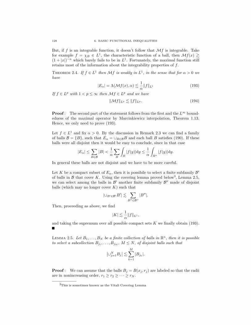
128 6. BASIC FUNCTIONAL INEQUALITIES
But, if f is an integrable function, it doesn’t follow that Mf is integrable. Takefor example f = χB ∈ L1, the characteristic function of a ball, then Mf(x) &(1 + |x|)−n which barely fails to be in L1. Fortunately, the maximal function stillretains most of the information about the integrability properties of f .
Theorem 2.4. If f ∈ L1 then Mf is weakly in L1, in the sense that for α > 0 wehave
|Eα| = Λ(Mf(x), α) .1
α‖f‖L1 (193)
If f ∈ Lp with 1 < p ≤ ∞ then Mf ∈ Lp and we have
‖Mf‖Lp . ‖f‖Lp . (194)
Proof : The second part of the statement follows from the first and the L∞ bound-edness of the maximal operator by Marcinkiewicz interpolation, Theorem 1.13.Hence, we only need to prove (193).
Let f ∈ L1 and fix α > 0. By the discussion in Remark 2.3 we can find a familyof balls B = B, such that Eα = ∪B∈BB and each ball B satisfies (190). If theseballs were all disjoint then it would be easy to conclude, since in that case
|Eα| ≤∑B∈B|B| < 1
α
∑B
∫B
|f(y)|dy ≤ 1
α
∫Rn|f(y)|dy.
In general these balls are not disjoint and we have to be more careful.
Let K be a compact subset of Eα, then it is possibile to select a finite subfamily B′of balls in B that cover K. Using the covering lemma proved below3, Lemma 2.5,we can select among the balls in B′ another finite subfamily B′′ made of disjointballs (which may no longer cover K) such that
|∪B′∈B′B′| .∑
B′′∈B′′|B′′|.
Then, proceeding as above, we find
|K| . 1
α‖f‖L1 ,
and taking the supremum over all possible compact sets K we finally obtain (193).
Lemma 2.5. Let B1, . . . , BN be a finite collection of balls in Rn, then it is possibleto select a subcollection Bj1 , . . . , BjM , M ≤ N , of disjoint balls such that
∣∣∪Nj=1Bj∣∣ . M∑
k=1
|Bjk |.
Proof : We can assume that the balls Bj = B(xj , rj) are labeled so that the radiiare in nonincreasing order, r1 ≥ r2 ≥ · · · ≥ rN .
3This is sometimes known as the Vitali Covering Lemma
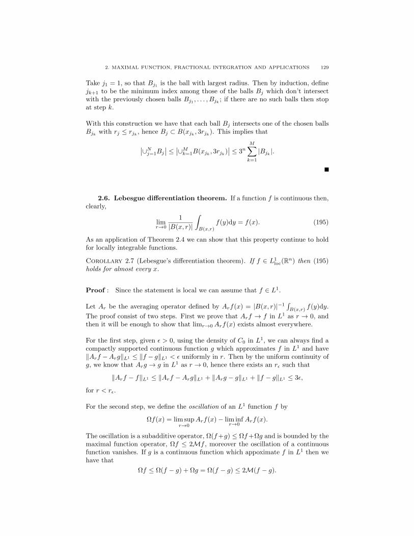
2. MAXIMAL FUNCTION, FRACTIONAL INTEGRATION AND APPLICATIONS 129
Take j1 = 1, so that Bj1 is the ball with largest radius. Then by induction, definejk+1 to be the minimum index among those of the balls Bj which don’t intersectwith the previously chosen balls Bj1 , . . . , Bjk ; if there are no such balls then stopat step k.
With this construction we have that each ball Bj intersects one of the chosen ballsBjk with rj ≤ rjk , hence Bj ⊂ B(xjk , 3rjk). This implies that
∣∣∪Nj=1Bj∣∣ ≤ ∣∣∪Mk=1B(xjk , 3rjk)
∣∣ ≤ 3nM∑k=1
|Bjk |.
2.6. Lebesgue differentiation theorem. If a function f is continuous then,clearly,
limr→0
1
|B(x, r)|
∫B(x,r)
f(y)dy = f(x). (195)
As an application of Theorem 2.4 we can show that this property continue to holdfor locally integrable functions.
Corollary 2.7 (Lebesgue’s differentiation theorem). If f ∈ L1loc(Rn) then (195)
holds for almost every x.
Proof : Since the statement is local we can assume that f ∈ L1.
Let Ar be the averaging operator defined by Arf(x) = |B(x, r)|−1∫B(x,r)
f(y)dy.
The proof consist of two steps. First we prove that Arf → f in L1 as r → 0, andthen it will be enough to show that limr→0Arf(x) exists almost everywhere.
For the first step, given ε > 0, using the density of C0 in L1, we can always find acompactly supported continuous function g which approximates f in L1 and have‖Arf −Arg‖L1 ≤ ‖f − g‖L1 < ε uniformly in r. Then by the uniform continuity ofg, we know that Arg → g in L1 as r → 0, hence there exists an rε such that
‖Arf − f‖L1 ≤ ‖Arf −Arg‖L1 + ‖Arg − g‖L1 + ‖f − g‖L1 ≤ 3ε,
for r < rε.
For the second step, we define the oscillation of an L1 function f by
Ωf(x) = lim supr→0
Arf(x)− lim infr→0
Arf(x).
The oscillation is a subadditive operator, Ω(f+g) ≤ Ωf+Ωg and is bounded by themaximal function operator, Ωf ≤ 2Mf , moreover the oscillation of a continuousfunction vanishes. If g is a continuous function which appoximate f in L1 then wehave that
Ωf ≤ Ω(f − g) + Ωg = Ω(f − g) ≤ 2M(f − g).
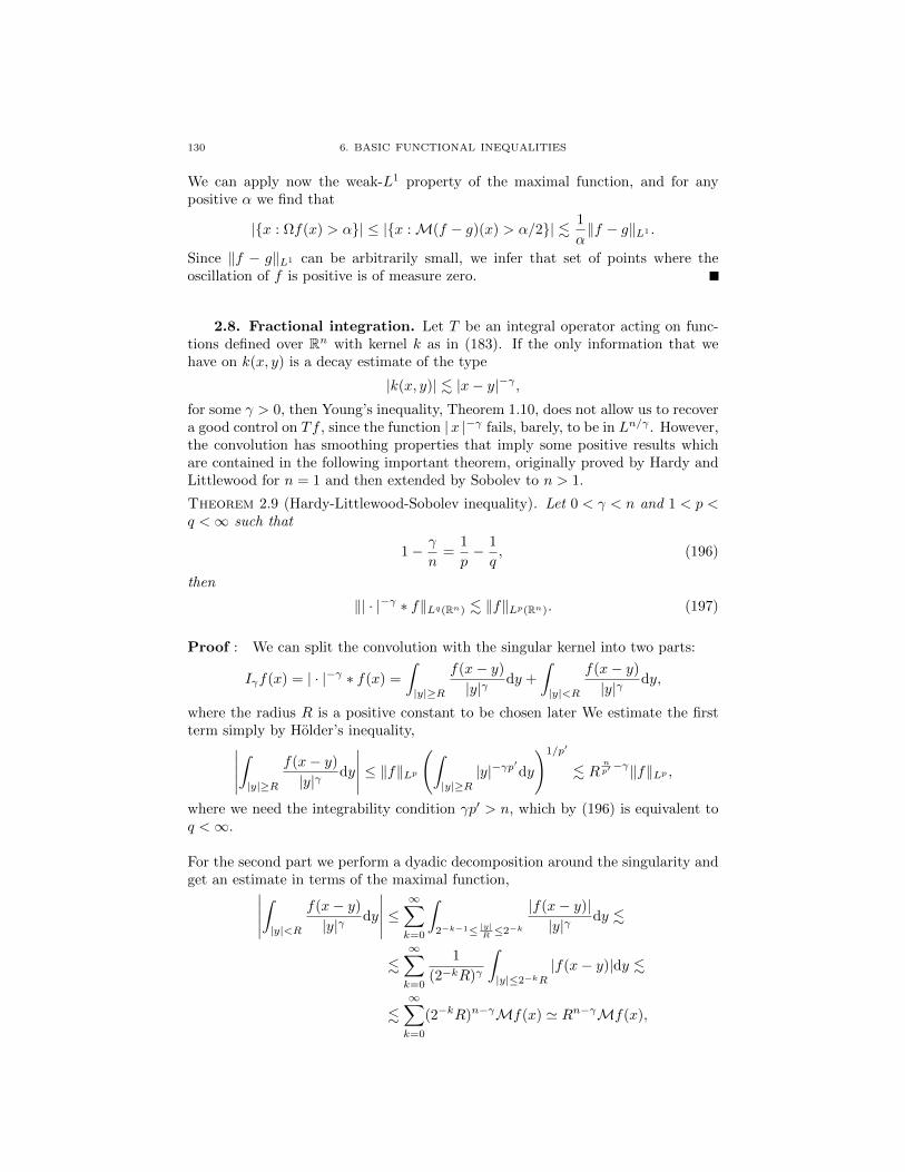
130 6. BASIC FUNCTIONAL INEQUALITIES
We can apply now the weak-L1 property of the maximal function, and for anypositive α we find that
|x : Ωf(x) > α| ≤ |x :M(f − g)(x) > α/2| . 1
α‖f − g‖L1 .
Since ‖f − g‖L1 can be arbitrarily small, we infer that set of points where theoscillation of f is positive is of measure zero.
2.8. Fractional integration. Let T be an integral operator acting on func-tions defined over Rn with kernel k as in (183). If the only information that wehave on k(x, y) is a decay estimate of the type
|k(x, y)| . |x− y|−γ ,for some γ > 0, then Young’s inequality, Theorem 1.10, does not allow us to recovera good control on Tf , since the function |x |−γ fails, barely, to be in Ln/γ . However,the convolution has smoothing properties that imply some positive results whichare contained in the following important theorem, originally proved by Hardy andLittlewood for n = 1 and then extended by Sobolev to n > 1.
Theorem 2.9 (Hardy-Littlewood-Sobolev inequality). Let 0 < γ < n and 1 < p <q <∞ such that
1− γ
n=
1
p− 1
q, (196)
then
‖| · |−γ ∗ f‖Lq(Rn) . ‖f‖Lp(Rn). (197)
Proof : We can split the convolution with the singular kernel into two parts:
Iγf(x) = | · |−γ ∗ f(x) =
∫|y|≥R
f(x− y)
|y|γdy +
∫|y|<R
f(x− y)
|y|γdy,
where the radius R is a positive constant to be chosen later We estimate the firstterm simply by Holder’s inequality,∣∣∣∣∣
∫|y|≥R
f(x− y)
|y|γdy
∣∣∣∣∣ ≤ ‖f‖Lp(∫|y|≥R
|y|−γp′dy
)1/p′
. Rnp′−γ‖f‖Lp ,
where we need the integrability condition γp′ > n, which by (196) is equivalent toq <∞.
For the second part we perform a dyadic decomposition around the singularity andget an estimate in terms of the maximal function,∣∣∣∣∣
∫|y|<R
f(x− y)
|y|γdy
∣∣∣∣∣ ≤∞∑k=0
∫2−k−1≤ |y|R ≤2−k
|f(x− y)||y|γ
dy .
.∞∑k=0
1
(2−kR)γ
∫|y|≤2−kR
|f(x− y)|dy .
.∞∑k=0
(2−kR)n−γMf(x) ' Rn−γMf(x),
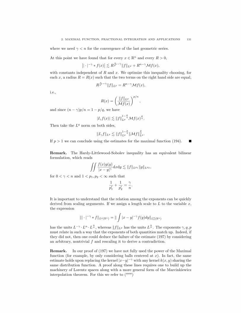
2. MAXIMAL FUNCTION, FRACTIONAL INTEGRATION AND APPLICATIONS 131
where we need γ < n for the convergence of the last geometric series.
At this point we have found that for every x ∈ Rn and every R > 0,∣∣| · |−γ ∗ f(x)∣∣ . R n
p′−γ‖f‖Lp +Rn−γMf(x),
with constants independent of R and x. We optimize this inequality choosing, foreach x, a radius R = R(x) such that the two terms on the right hand side are equal,
Rnp′−γ‖f‖Lp = Rn−γMf(x),
i.e.,
R(x) =
(‖f‖LpMf(x)
)p/n,
and since (n− γ)p/n = 1− p/q, we have
|Iγf(x)| . ‖f‖1−pq
Lp Mf(x)pq .
Then take the Lq norm on both sides,
‖Iγf‖Lq . ‖f‖1− pqLp ‖Mf‖
pq
Lp .
If p > 1 we can conclude using the estimates for the maximal function (194).
Remark. The Hardy-Littlewood-Sobolev inequality has an equivalent bilinearformulation, which reads∫∫
f(x)g(y)
|x− y|γdxdy . ‖f‖Lp1‖g‖Lp2 ,
for 0 < γ < n and 1 < p1, p2 <∞ such that
1
p′1+
1
p′2=γ
n.
It is important to understand that the relation among the exponents can be quicklyderived from scaling arguments. If we assign a length scale to L to the variable x,the expression
‖| · |−γ ∗ f‖Lq(Rn) = ‖∫|x− y|−γf(y)dy‖Lqx(Rn)
has the units L−γ ·Ln ·Lnq , whereas ‖f‖Lp has the units L
np . The exponents γ, q, p
must relate in such a way that the exponents of both quantities match up. Indeed, ifthey did not, then one could deduce the failure of the estimate (197) by consideringan arbitrary, nontrivial f and rescaling it to derive a contradiction.
Remark. In our proof of (197) we have not fully used the power of the Maximalfunction (for example, by only considering balls centered at x). In fact, the sameestimate holds upon replacing the kernel |x−y|−γ with any kernel k(x, y) sharing thesame distribution function. A proof along these lines requires one to build up themachinery of Lorentz spaces along with a more general form of the Marcinkiewiczinterpolation theorem. For this we refer to (***)
132 6. BASIC FUNCTIONAL INEQUALITIES
Using the Hardy-Littlewood-Sobolev inequality, we now show that it is possible togive a very short proof of the Sobolev inequality,
‖f‖Lq . ‖∂f‖Lp ,
for n/q = n/p − 1, in the non sharp regime p > 1. As with the Hardy-LittlewoodSobolev inequality, the exponents are easily deduced by considering the lengthscaling of both sides. The Sobolev inequality quantifies the intuitive fact that afunction can only blow up somewhere if its derivatives blow up even worse.
Proof. Assume f ∈ C∞0 (Rn). For every unit vector ω we have
f(x) = −∫ ∞
0
d
drf(x+ ωr)dr
To consider all possible directions in which f could grow, we integrate over thewhole sphere, and recalling that the volume element in Rn in polar coordinates isdy = rn−1drdσω, we find that
|f(x)| .∫|∂f(y)||x− y|n−1
dy =(| · |1−n ∗ |∂f |
)(x).
We take the Lq norm and use (197) to get
‖f‖Lq . ‖ | · |1−n ∗ |∂f | ‖Lq . ‖ ∂f ‖Lp ,
whenever p > 1 and
1− n− 1
n=
1
p− 1
q.
2.10. Sobolev Inequalities. In the previous section we have seen how toestimate the Lq(Rn) norm of a function in terms of an Lp norm, 1− n−1
n = 1p −
1q ,
p > 1, of the gradient of f . We shall now prove a stronger version of this.
Theorem 2.11 (Galgliardo-Nirenberg-Sobolev). The inequality
‖f‖Lq(Rn) . ‖∂mf‖Lp(Rn), f ∈ C∞0 (Rn), (198)
holds for
1
q=
1
p− m
n> 0, m ∈ N, (1 ≤ p < q <∞). (199)
While for q =∞, we have
‖f‖L∞(Rn) .m∑k=0
‖∂kf‖Lp(Rn), f ∈ C∞0 (Rn), (200)
when np −m < 0.
Remark. We don’t need to remember the precise condition (199); it can be de-duced by a simple dimensional analysis. Since the estimate is homogeneous, it hasto be invariant under dilations, and (199) simply says that both sides in (198) havethe same scaling. Also the condition n
p −m < 0 is a comparison of the scalings of
the two sides of (200) which excludes a very localized and spiky counterexample.
2. MAXIMAL FUNCTION, FRACTIONAL INTEGRATION AND APPLICATIONS 133
Remark. The following non-sharp version of estimate (198) also holds for all1 ≤ p < q <∞ and 1/p−m/n < 1/q,
‖f‖Lq(Rn) .∑|α|≤m
‖∂αf‖Lp f ∈ C∞0 (Rn), (201)
Exercise. Show by an example that the inequality (200) can fail to be true forp = n/m. Prove (201) for m = 1, using the results of theorem 2.11.
Exercise. Show by a scaling argument that if the inequality (201) holds true for1/p = 1/q +m/n < 0 then the homogeneous inequality (198) is also true.
Proof [Proof of (198)]: We obtain the cases with m > 1 by repeated iterations ofthe case m = 1. Hence, we can assume m = 1 and, by (199),
1 ≤ p < n,n
n− 1≤ q =
np
n− p<∞.
Once we have the estimate for p = 1 and q = n/(n − 1), then we get the caseswith p > 1 and q > n/(n − 1) by simply applying Holder inequality. Indeed, letq = λn/(n− 1), for some λ > 1, then
‖f‖λLq = ‖|f |λ‖L
nn−1. ‖|f |λ−1∂f‖L1 ≤ ‖|f |λ−1‖Lp′‖∂f‖Lp ,
and we just have to check that
(λ− 1)p′ =n−1n q − 1
1− 1n −
1q
= q.
But this essentially needs no verification – by the scaling of the inequality, theexponents must work out.
It only remains to prove the special case m = 1, p = 1, q = n/(n − 1). FollowingNirenberg, [?], one can show the stronger result that for f ∈ C∞0 (Rn) we have
‖f‖L
nn−1 (Rn)
.n∏j=1
‖∂jf‖1/nL1(Rn). (202)
When n = 1, this comes easily from writing
f(x) =
∫ x
−∞f ′(y)dy.
When n = 2, we do the same with respect toeach variable and then multiply andintegrate:∫∫
|f(x1, x2)|2dx1dx2 ≤∫∫ ∫
|∂1f(y1, x2)|dy1
∫|∂2f(x1, y2)|dy2dx1dx2
= ‖∂1f‖L1‖∂2f‖L1 .
When n ≥ 3 things become more tricky and, to separate the variables, we have tomake a repeated use of Holder inequality. Let just look at the case n = 3. To ease
134 6. BASIC FUNCTIONAL INEQUALITIES
the notation set fj = ∂jf and∫φ(x)dxj =
∫jφ(xj). We start with
|f(x)| 32 ≤(∫
1
|f1(·, x2, x3)|) 1
2(∫
2
|f2(x1, ·, x3)|) 1
2(∫
3
|f3(x1, x2, ·)|) 1
2
.
Then integrate with respect to x1. The first factor on the right hand side doesn’tdepend on x1, while we use Holder to separate the second from the third,∫
1
|f(·, x2, x3)| 32 ≤(∫
1
|f1(·, x2, x3)|) 1
2(∫
1,2
|f2(·, ·, x3)|) 1
2(∫
1,3
|f3(·, x2, ·)|) 1
2
.
Proceed similarly with the integration with respect tox2,∫1,2
|f(·, ·, x3)| 32 ≤(∫
1,2
|f1(·, ·, x3)|) 1
2(∫
1,2
|f2(·, ·, x3)|) 1
2(∫
1,2,3
|f3(·)|) 1
2
,
and finally do the same with x3,∫1,2,3
|f(·)| 32 ≤(∫
1,2,3
|f1(·)|) 1
2(∫
1,2,3
|f2(·)|) 1
2(∫
1,2,3
|f3(·)|) 1
2
.
When n > 3 the procedure is exacly the same.
Proof [Proof of (200)]: It clearly suffices to look at the case m = 1, since thecases m > 1 will follow from it applying (198). Assume thus m = 1 and p > n, wewant to prove that
|f(0)| . ‖f‖Lp + ‖Df‖Lp .
Suppose first that f has support contained in the unit ball B = |x| < 1, then
f(0) = −∫ 1
0
d
drf(rω)dr, ω ∈ Sn−1. (203)
Integrate with respect toω and then apply Holder,
|f(0)| .∫B
|∂f(x)||x|n−1
dx . ‖∂f‖Lp(∫
B
dx
|x|(n−1)p′
)1/p′
. ‖∂f‖Lp ,(204)
where the integrability condition needed here is (n − 1)p′ < n, which is preciselyp > n.
In general, fix a cutoff function φ ∈ C∞0 with support in B and φ(0) = 1, then inview of the above, |f(0)| = |φ(0)f(0)| . ‖∂(φf)‖Lp . ‖f‖Lp + ‖∂f‖Lp .
2.12. Classical Sobolev spaces. The Sobolev inequalities of theorem (2.11)lead us to the introduction of Sobolev spaces.
Definition 2.13. Let Ω be an open subset of Rn. Fix 1 ≤ p ≤ ∞ and let s ∈ Nbe a non-negative integer. The space W s,p(Ω) consists of all locally integrable, real(or complex) valued functions u on Ω such that for all multiindex α with |α| ≤ s
2. MAXIMAL FUNCTION, FRACTIONAL INTEGRATION AND APPLICATIONS 135
the weak4 derivatives ∂αu belong to Lp(Ω). These spaces come equiped with thenorms,
‖u‖W s,p(Ω) =( ∑|α|≤s
‖∂αu‖pLp(Ω)
)1/p, for 1 ≤ p <∞
‖u‖W s,∞(Ω) =∑|α|≤s
‖∂αu‖L∞(Ω)
We also denote by W k,p0 (Ω) the closure of C∞0 (Ω) in W k,p(Ω).
In the particular case p = 2 we write Hs(Ω) = W s,2(Ω). Clearly H0(Ω) = L2(Ω).
We also write Hs0(Ω) = W s,2
0 (Ω). These spaces are especially important because oftheir Hilbert space structure.
In the particular case p = ∞ we work with the smaller space Cs(Ω) ⊂ W s,∞(Ω),the set of functions which are s times continuously differentiable and have bounded‖ ‖W s,∞ norm.
Exercise. Show that for each s ∈ N and 1 ≤ p ≤ ∞ the spaces W s,p(Ω) areBanach spaces.
There is a lot more to be said about Sobolev spaces in domains Ω ⊂ Rn. Forinstance, We refer the reader to Evans ([E], ch. 5). For the time being we specializeto the case Ω = Rn.
Exercise. Show that the spaces W k,p(Rn) and W k,p0 (Rn) coincide. That means
that C∞0 is dense in W k,p(Rn).
The Sobolev inequalities proved in the previous subsection can be interpreted asembedding theorems. Indeed (198) and (201) can be interpreted as saying thatthe Sobolev space Wm,p(Rn) is included in the Lebesgue space Lq(Rn) as long as1p −
mn ≤
1q .
Proposition 2.14. The following inclusions are continuous
Wm,p(Rn) ⊂ Lq(Rn), if1
p− m
n≤ 1
q.
Moreover, for q = ∞, Wm,p(Rn) embeds into the space of bounded continuousfunctions on Rn provided that m > n/p.
Proof : Follows from theorem 2.11 and the density of C∞0 (Rn) in Wm,p(Rn).
2.15. Holder spaces. Together with Sobolev spaces Holder spaces play a veryimportant role in Analysis, especially in connection to elliptic equations. Beforeintroducing these spaces we recall the definitions of the spaces Cm(Ω) of m times
4That is derivatives in the sense of distributions.
136 6. BASIC FUNCTIONAL INEQUALITIES
continuously differentiable functions u : Ω→ R on an open domain Ω for which theWm,∞ norm is bounded,
‖u‖Cm(Ω) =∑|α|≤m
‖∂αu(x)‖L∞(Ω) <∞.
Definition 2.16. Let Ω be an open domain in Rn. We say that a function u : Ω→R is Holder continuous with exponent 0 < γ ≤ 1 if,
[u]C0,γ(Ω) = supx 6=y∈Ω
|u(x)− u(y)||x− y|γ
<∞. (205)
The Holder space Ck,γ(Ω) consists of all functions u ∈ Ck(Ω) for which the norm,
‖u‖Ck,γ(Ω) = ‖u‖Ck(Ω) +∑|α|=k
[∂αu]C0,γ(Ω). (206)
is finite.
Exercise 2.17. The space Ck,γ(Ω) is a Banach space.
Exercise 2.18. Show that C0,1((a, b)), the space of Lipschitz functions on aninterval, consists exactly of those distributions whose derivative belongs to L∞.
Exercise 2.19. Let f(x) = (a ≤ x ≤ b) be the characteristic function of aninterval. Show that the seven-fold convolution f ∗ · · · ∗f is in the Holder class C5,1.
The following stronger version of the Sobolev embedding in L∞ is important inelliptic theory. As usual, the relationship between the exponents involved can bededuced from dimensional analysis.
Theorem 2.20 (Morrey’s inequality). Assume n < p ≤ ∞. Then, for all u ∈C∞0 (Rn),
‖u‖C0,γ(Rn) . ‖u‖W 1,p(Rn) (207)
provided that γ = 1− n/p.
Proof : In one dimension, this is an easy application of the fundamental theoremof calculus and Holder’s inequality. For the general case, see [E], section 5.6.2.
2.21. Fractional Hs- Sobolev spaces. Consider the Sobolev space
Hs(Rn) = u ∈ L2 : ∂αu ∈ L2, ∀ |α| ≤ s.
Proposition 2.22. The Sobolev space Hs(Rn) coincides with the set of all tempereddistributions u ∈ S ′(RN ) for which u is locally integrable and,
‖u‖2Hs =
∫RN
(1 + |ξ|2)s|u(ξ)|2 <∞ (208)
2. MAXIMAL FUNCTION, FRACTIONAL INTEGRATION AND APPLICATIONS 137
Proof : Follows easily from the Parseval identity, the density of C∞0 in each space,
and the fact that ∂jf(ξ) = iξj f(ξ).
Observe that the equivalent definition of proposition 2.22 makes sense not only forpositive integers but for all real numbers s. We can thus talk about Sobolev spacesHs for all real values of s. We shall also make use of the following homogeneousSobolev norm, for all s ≥ 0,
‖u‖2Hs
=
∫RN|ξ|2s|u(ξ)|2 <∞ (209)
Question. Why does ‖u‖Hs have units LN2 −s if we consider the physical space
variable to have the unit L?
Exercise. For s ∈ (0, 1) the space Hs(Rn) coincides with the space of locallyintegrable functions such that,(∫
Rn
∫Rn
|u(x)− u(x+ y)|2
|y|n+2sdxdy + ‖u‖2L2(Rn)
)1/2
<∞ (210)
Exercise. Prove that, for s > n/2 the Sobolev space Hs(Rn) embeds in the spaceof bounded continuous functions.
2.23. A Trace Theorem. In order to make sense of boundary values of gen-eralized functions for partial differential equations, it is important to prove that theoperation of restriction, which obviously makes sense for continuous functions, con-tinues to make sense even when the function is not continuous. Such theorems arecalled trace theorems. Consider, for simplicity, the case of the hyperplane xn = 0in Rn and define the trace operator,
Tf(x1, . . . , xn) = f(x1, . . . , xn−1, 0). (211)
Clearly the operator makes sense for any continuous functions f , in particular forany test function, in Rn.
Theorem 2.24. The following estimate holds true, uniformly for any test functionf ∈ C∞0 (Rn), n ≥ 2 and any s > 1/2.
‖Tf‖Hs−
12 (Rn−1)
. ‖f‖Hs(Rn) (212)
Therefore T extends as a linear map T : Hs(Rn)→ Hs−1/2(Rn−1).
Remark. Observe that the result is dimensionally sharp, which is somewhat sur-prising if one compares it to the usual embedding of the Sobolev spaces Hs(R) inL∞(R), in which case we know that the sharp case, s = 1/2, is false. In fact theabove trace theorem is also false for the case s = 1/2.
Proof : Take f smooth and g(x′) = f(x′, 0). Let f be the Fourier transform of f in
xn only, and f , g be the Fourier transforms of f and g in Rn and Rn−1, respectively.
138 6. BASIC FUNCTIONAL INEQUALITIES
I.e.
f(x′, ξn) =
∫ ∞−∞
f(x′, xn)e−ixnξndxn
By applying Fourier inversion (with xn = 0) and then the Fourier transform, weget
g(x′) = f(x′, 0) =1
2π
∫ ∞−∞
f(x′, ξm)dξn
g(ξ′) =1
2π
∫ ∞−∞
f(ξ′, ξm)dξn
We can then see, using our knowledge of fractional Hs spaces and Cauchy-Schwartz:
‖g‖Hs−1/2(Rn−1 .∫Rn−1
|g(ξ′)|2(1 + |ξ′|2)s−1/2dξ′
.∫Rn−1
∣∣∣∣∫ ∞−∞
f(ξ)dξn
∣∣∣∣2 (1 + |ξ′|2)s−1/2dξ′
.∫Rn−1
(1 + |ξ′|2)s−1/2
(∫ ∞−∞|f(ξ)|2(1 + |ξ|2)sdξn
)J(ξ′)dξ′
with,
J(ξ′) =
∫ ∞−∞
(1 + |ξ|2)−sdξn
And since s > 1/2, we have
J(ξ′) =
∫ ∞−∞
(1 + |ξ|2)−sdξn =
∫ ∞−∞
(1 + |ξ′|2 + |ξn|2)−sdξn
= (1 + |ξ′|2)−s+1/2
∫ ∞−∞
(1 + y2)−sdy
Plugging this into our above estimate for ‖g‖Hs−1/2 proves the result.
Similar results hold for traces to higher co-dimension hypersurfaces. Here is sucha result, which can be proved by elementary means.
Proposition 2.25. Consider the trace operator T in R3 which takes continuousfunctions f(t, x1, x2) to Tf(t) = f(t, 0, 0). We have, for any test function f ,
‖∂t(Tf)‖L2(R) . ‖∂2f‖L2(R3) (213)
Thus, T extends, as a bounded linear operator, to H2(R3) with values in H1(R).
Proof∫R|∂tf(t, 0, 0)|2dt =
∫ ∞0
dx1
∫ ∞0
dx2(∂1∂2
∫R∂tf(t, x)∂tf(t, x)dt
)= 2
∫ ∞0
dx1
∫ ∞0
dx2( ∫
R∂1∂2∂tf(t, x)∂tf(t, x)dt
)+ 2
∫ ∞0
dx1
∫ ∞0
dx2( ∫
R∂1∂tf(t, x)∂2∂tf(t, x)dt
)
2. MAXIMAL FUNCTION, FRACTIONAL INTEGRATION AND APPLICATIONS 139
Clearly,∣∣∣∣ ∫ ∞0
dx1
∫ ∞0
dx2( ∫−∞
∂1∂tf(t, x)∂2∂tf(t, x)dt)∣∣∣∣ . ‖∂2f‖2L2(R3)
On the other hand, integrating by parts in t,∫R∂1∂2∂tf(t, x)∂tf(t, x)dt = −
∫R∂1∂2f(t, x)∂2
t f(t, x)dt
Hence, ∣∣∣∣ ∫ ∞0
dx1
∫ ∞0
dx2( ∫−∞
∂1∂2∂tf(t, x)∂tf(t, x)dt)∣∣∣∣ . ‖∂2f‖L2(R3).
as desired.
Exercise. Prove the same result using Fourier transform and extend it to all di-mensions and generalHs spaces. Exercise Extend the result to bounded intervalsin t.
2.26. Extensions. To extend results which hold true for functions in Rn todomains in Rn we need to extend the functions in a controlled manner. I will restrictthe discussion to the case of the half space Rn+ = x ∈ Rn/xn ≥ 0. Consider theSobolev space W 1,p(Rn+). We want to prove the following.
Proposition 2.27. There exists a bounded linear operator E : W 1,p(Rn+)→W 1,p(Rn),such that for any continuous f ,
Ef |Rn+ = f
and,
‖Ef‖W 1,p(Rn) . ‖f‖W 1,p(Rn+)
Proof It suffices to prove the result for functions f ∈ C1(Rn+). Given such a func-tion we define, using its higher order reflection, its extension barf which coincidedwith f in Rn+ and, for all xn < 0,
f(x′, xn) = −3f(x′,−xn) + 4f(x′,−1
2xn)
Observe first that f is also C1. Indeed f is continuous across xn = 0 and so are itsderivatives with respect to the variables x′ = (x1, . . . , xn−1). On the other hand,for xn < 0,
∂nf(x′, xn) = 3∂nf(x′,−xn)− 2∂nf(x′,−1
2xn)
Hence, letting xn tend to zero with xn < 0
(∂nf)−(x′, 0) = ∂nf(x′, 0).
Using these calculations we immediately derive the desired estimate.
140 6. BASIC FUNCTIONAL INEQUALITIES
Exercise Extend the result to the W s,p spaces, with s ∈ N. What about fractionalHs spaces ?.
3. Littlewood-Paley theory
In its simplest manifestation Littlewood-Paley theory is a systematic and very use-ful method to understand various properties of functions f , defined on Rn, bydecomposing them in infinite dyadic sums f =
∑k∈Z fk, with frequency local-
ized components fk, i.e. fk(ξ) = 0 for all values of ξ outside the dyadic annulus2k−1 ≤ |ξ| ≤ 2k+1. Such a decomposition can be easily achieved by choosing a testfunction χ(ξ) in Fourier space, supported in 1
2 ≤ |ξ| ≤ 2, and such that, for allξ 6= 0, ∑
k∈Zχ(2−kξ) = 1. (214)
Indeed choose φ(ξ) to be a real radial bump function supported in |ξ| ≤ 2 whichequals 1 on the ball |ξ| ≤ 1. Then the function χ(ξ) = φ(ξ) − φ(2ξ) verifies thedesired properties.
We now define
Pkf(ξ) = χ(ξ/2k)f(ξ) (215)
or, in physical space,
Pkf = fk = mk ∗ f (216)
where mk(x) = 2nkm(2kx) and m(x) the inverse Fourier transform of χ. Clearly,from (214)
f =∑k∈Z
Pkf (217)
as desired. Denoting the map “multiplication by 2−k” by 2−k, we also have theimportant scaling identity
(Pkf) 2−k = P0(f 2−k) (218)
Observe that the Fourier transform of Pkf is supported in the dyadic interval2k−1 ≤ |ξ| ≤ 2k+1 and therefore,
Pk′Pkf = 0, ∀ k, k′ ∈ Z, |k − k′| > 2.
Therefore,
Pkf =∑k′∈Z
Pk′(Pkf) =∑
|k−k′|≤1
Pk′Pkf
Thus, since Pk−1, Pk, Pk+1 do not differ much between themselves we can writePk =
∑|k−k′|≤1 Pk′Pk ≈ P 2
k . It is for this reason that the cut-off operators Pk are
called, improperly, LP projections.
Denote PJ =∑k∈J Pk for all intervals J ⊂ Z. We write, in particular, P≤k =
P(−∞,k] and P<k = P≤k−1. Clearly, Pk = P≤k − P<k.
3. LITTLEWOOD-PALEY THEORY 141
The following properties of these LP projections lie at the heart of the classical LPtheory:
Theorem 3.1. The LP projections verify the following properties:
LP 1. Almost Orthogonality. The operators Pk are selfadjoint and verifyPk1
Pk2= 0 for all pairs of integers such that |k1 − k2| ≥ 2. In particular,
‖f‖2L2 ≈∑k
‖Pkf‖2L2 (219)
LP 2. Lp-boundedness: For any 1 ≤ p ≤ ∞, and any interval J ⊂ Z,
‖PJf‖Lp . ‖f‖Lp (220)
LP 3. Finite band property. We can write any partial derivative ∂Pkf in theform ∂Pkf = 2kPkf and the symbol of Pk is a cut-off operator5 which verifiesproperty LP2. In particular, for any 1 ≤ p ≤ ∞
‖∂Pkf‖Lp . 2k‖f‖Lp (221)
2k‖Pkf‖Lp . ‖∂f‖Lp (222)
LP 4. Bernstein inequalities. For any 1 ≤ p ≤ q ≤ ∞ we have the Bernsteininequalities,
‖Pkf‖Lq . 2kn(1/p−1/q)‖f‖Lp , ∀ k ∈ Z (223)
‖P≤0f‖Lq . ‖f‖Lp . (224)
In particular,
‖Pkf‖L∞ . 2kn/p‖f‖Lp .
LP5. Commutator estimates Consider the commutator
[Pk , f ] · g = Pk(f · g)− f · Pkg
with f, g ∈ C∞0 (Rn). We have,
‖ [Pk , f ] · g‖Lp . 2−k‖∇f‖L∞‖g‖Lp .
LP6. Square function inequalities. Let Sf be the vector valued function Sf =(Pkf)k∈Z. The quantity
Sf(x) = |Sf(x)| =(∑k∈Z|Pkf(x)|2
)1/2(225)
is known as the Littlewood-Paley square function. For every 1 < p <∞ there existsconstant(s), depending on p, such that for all f ∈ C∞0
‖f‖Lp . ‖Sf‖Lp . ‖f‖Lp (226)
5Associated with a slightly different test function χ which remains supported in 12≤ |ξ| ≤ 2,
but may fail to satisfy (214).
142 6. BASIC FUNCTIONAL INEQUALITIES
Proof : Only the proof of LP6 is not straightforward and we postpone it untilnext section. The proof of LP1 is immediate. Indeed we only have to check (219).Clearly,
‖f‖2L2 = ‖∑k
Pkf‖2L2 =∑
|k−k′|≤1
< Pkf, Pk′f >L2
≤∑
|k−k′|≤1
‖Pkf‖L2‖Pk′f‖L2
.∑k
‖Pkf‖2L2
To show that∑k ‖Pkf‖2L2 . ‖f‖2L2 we only need to use Parseval’s identity together
with the definition of the projections Pk.
It suffices to prove LP2 for intervals of the form J = (−∞, k] ⊂ Z, that is to prove
Lp boundedness for P≤k. If χ(ξ) = φ(ξ)− φ(2ξ) then P≤kf = φ(ξ/2k)f(ξ). Thus
P≤kf = mk∗f,
where mk(x) = 2nkm(2kx) and m(x) is the inverse Fourier transform of φ. Observethat ‖mk‖L1 = ‖m‖L1 . 1. Thus, using the convolution inequality (188),
‖P≤kf‖Lp ≤ ‖mk‖L1‖f‖Lp . ‖f‖Lp
as desired.
To prove LP3 we write ∂i(Pkf) = 2k(∂im)k∗f where (∂im)k(x) = 2nk∂im(2kx).Clearly ‖(∂im)k‖L1 = ‖∂im‖L1 . 1. Hence,
‖∂i(Pkf)‖Lp . 2k‖f‖Lp
which establishes (221). To prove (222) we write f(ξ) =∑nj=1
ξji|ξ|2 ∂xjf(ξ). Hence,
2kPkf(ξ) =
n∑j=1
2kξji|ξ|2
χ(ξ/2k)∂xjf(ξ) =
n∑j=1
2kψj(ξ/2k)∂xjf(ξ)
where ψj(ξ) =ξji|ξ|2χ(ξ). Hence, in physical space,
2kPkf =
n∑j=1
(jm)k∗∂jf
with (jm)k(x) = 2nk · jm(2kx) and jm the inverse Fourier transform of ψj . Thus,as before,
2k‖Pkf‖Lp .n∑j=1
‖∂jf‖Lp = ‖∂f‖Lp
as desired.
Property LP4 is an immediate consequence of the physical space representation(216) and the convolution inequality (188).
‖Pkf‖Lq = ‖mk∗f‖Lq . ‖mk‖Lr‖f‖Lp
3. LITTLEWOOD-PALEY THEORY 143
where 1 + q−1 = r−1 + p−1. Now,
‖mk‖Lr = 2nk( ∫
Rn|m(2kx)|rdx
)1/r= 2nk2−nk/r‖m‖Lr . 2nk(1−1/r) . 2nk(1/p−1/q)
It only remains to prove LP5. In view of (216) we can write,
Pk(fg)(x)− f(x)Pkg(x) =
∫Rnmk(x− y)
(f(y)− f(x)
)g(y)dy
On the other hand,
|f(y)− f(x)| .∣∣ ∫ 1
0
d
dsf(x+ s(y − x))ds
∣∣. |x− y|‖∂f‖L∞
Hence,
|Pk(fg)(x)− f(x)Pkg(x)| . 2−k‖∂f‖L∞∫Rn|mk(x− y)||g(y)|dy
where mk(x) = 2nkm(2kx) and m(x) = |x|m(x). Thus,
‖Pk(fg)− fPkg‖Lp . 2−k‖∂f‖L∞‖g‖Lp
We leave the proof of property LP6 for the next section.
Remark. It could have simplified matters in the preceding proof to prove prop-erties LP2-4 only in the case k = 0, and deduce the more general estimates fromthe scaling identity (218). In particular, note that the Bernstein inequality is sim-ply the statement that lower Lp norms control higher Lp norms when f is localizedin frequency space (as opposed to the other way around, which occurs when f islocalized in physical space). This accords with our intuition for Lp norms: whilea frequency localized function may be too large at ∞ in physical space to be inte-grable, one need not worry about sudden jumps or spikes where the function blowsup locally, and hence only the former phenomenon needs to be controlled.
Definition. We say that a Fourier multiplier operator Pk is similar to a standardLP projection Pk if its symbol χk is a bump function adapted to the dyadic region|ξ| ∼ 2k. More precisely we can write χk(ξ) = χ( ξ
2k) for some bump function χ
supported in the region c−12k . |ξ| ≤ c2k for some fixed c > 0.
Remark. Observe that the inequality ‖Pkf‖Lp . ‖f‖Lp holds for every other
operator Pk similar to Pk. The same holds true for the properties LP3, LP4 andLP5.
Remark: We have the following pointwise relation of the operator Pk with themaximal function:
|P≤kf | .Mf(x) (227)
Indeed we have, as before,
P≤kf = mk∗f,
144 6. BASIC FUNCTIONAL INEQUALITIES
where mk(x) = 2nkm(2kx) and m(x) ∈ S(Rn). Therefore,
|P≤kf | . 2nk∫|f(y)|m
(2k(x− y)
)|dy . 2nk
∫|f(y)|(1 + 2k|x− y|)−n−1dy
. 2nk∫B(x,2−k)
|f(y)|(1 + 2k|x− y|)−n−1dy
+ 2nk∞∑j=0
∫2j≤2k|x−y|≤2j+1
|f(y)|(1 + 2k|x− y|)−n−1dy
. 2nk( ∫
B(x,2−k)
|f(y)|dy +∑j≥0
2−(n+1)j
∫|x−y|≤2j+1−k
|f(y)|dy)
. Mf(x) +∑j>0
2−(n+1)j2nk2n(j+1−k) 1
|B(x, 2−k+j+1)|
∫B(x,2−k+j+1)
|f(y)|dy
. Mf(x) + 2n∑j>0
2−jMf(x) .Mf(x)
as desired.
Properties LP3-LP4 go a long way to explain why LP theory is such a useful toolfor partial differential equations. The finite band property allows us to replacederivatives of the dyadic components fk by multiplication with 2k. The Lp → L∞
Bernstein inequality is a dyadic remedy for the failure of the embedding of theSobolev space W
np ,p(Rn) to L∞(Rn). Indeed, in view of the finite band property,
the Bernstein inequality does actually imply the desired Sobolev inequality for eachLP component fk, the failure of the Sobolev inequality for f is due to the summationf =
∑k fk.
In what follows we give a few applications of LP -calculus.
3.2. Interpolation inequalities. The following inequality holds true forarbitrary functions in C∞0 (Rn) and any integers 0 ≤ i ≤ m:
‖∂if‖Lp . ‖f‖1−i/mLp ‖∂mf‖i/mLp (228)
To prove it we decompose f = P≤kf + P>kf = f≤k + f>k. Now, using LP2-LP4,for any fixed value of k ∈ Z,
‖∂if‖Lp ≤ ‖∂if≤k‖Lp + ‖∂if>k‖Lp≤ 2ki‖f‖Lp + 2k(i−m)‖∂mf‖Lp
Thus,
‖∂if‖Lp ≤ λi‖f‖Lp + λi−m‖∂mf‖Lp
for any λ ∈ 2Z. To finish the proof we would like to choose λ such that the twoterms on the right hand side are equal to each other, i.e.,
λ0 =
(‖∂mf‖Lp‖f‖Lp
)1/m
3. LITTLEWOOD-PALEY THEORY 145
since we are restricted to λ ∈ 2Z we choose the dyadic number λ ∈ 2Z such that,λ ≤ λ0 ≤ 2λ Hence,
‖∂if‖Lp ≤ λi0‖f‖Lp +( 2
λ0
)m−i‖∂mf‖Lp . ‖f‖1−i/mLp ‖∂mf‖i/mLp .
In general when an estimate for functions on Rn fails to be dimensionally consistent(in that the scalings of the two sides are not the same), such an estimate can be“amplified” into one which appears even stronger (or proven false).
Exercise. Assuming the inequality
‖∂if‖Lp . ‖f‖Lp + ‖∂mf‖Lpdeduce the estimate (228) by considering the rescalings f → f λ.
3.3. Non-sharp Sobolev inequalities. We shall prove the following slightlyimproved version of the inequality (201), for functions f ∈ C∞0 (Rn) and exponents1 ≤ p < q <∞ with 1/p−m/n < 1/q,
‖f‖Lq(Rn) . ‖f‖Lp + ‖∂mf‖LpWe decompose f = P≤0f+
∑k∈N Pkf = f<0 +
∑k>0 fk. Thus, using LP4 and then
LP3,
‖f‖Lq ≤ ‖f<0‖Lq +∑k>0
‖fk‖Lq . ‖f‖Lp +∑k>0
2kn(1/p−1/q)‖f‖Lp
. ‖f‖Lp +∑k>0
2kn(m/n−ε)‖f‖Lp . ‖f‖Lp +∑k>0
2−knε‖∂mf‖Lp
. ‖f‖Lp + ‖∂mf‖Lp
3.4. Spaces of functions. The Littlewood-Paley theory can be used both togive alternative descriptions of Sobolev spaces and introduce new, more refined,spaces of functions. We first remark that, in view of the almost orthogonalityproperty LP1,
‖f‖2L2 = ‖∑k∈Z
Pkf‖2L2 .∑k∈Z‖Pkf‖2L2∑
k∈Z‖Pkf‖2L2 . ‖f‖L2
We can thus give an LP description of the homogeneous Sobolev norms ‖ ‖Hs(Rn)
‖f‖2Hs≈∑k∈Z
22ks‖Pkf‖2L2 (229)
For k ∈ Z+, define operator ∆k = Pk if k > 0, and ∆0 = P≤0. Also for the Hs
norms,
‖f‖2Hs ≈∞∑k=0
22ks‖∆kf‖2L2 (230)
The Littlewood- Paley decompositions can be used to define new spaces of functionssuch as Besov spaces.
146 6. BASIC FUNCTIONAL INEQUALITIES
Definition: The Besov space Bsp,q(Rn) is the closure of C∞0 (Rn) relative to thenorm:
‖f‖Bsp,q = (
∞∑k=0
2ksq‖∆kf‖qLp)1q (231)
The corresponding homogeneous Besov norm is defined by,
‖f‖Bsp,q = (∑k∈Z
2sqk‖Pkf‖qLp)1q , (232)
One similarly define Triebel space F sp,q by reversing the Lp norm and lq norm in(231). Thus, for example, the Hs norm is equivalent with the Besov norm Bs2,2.Observe that, Hs ⊂ Bs2,1. One reason why the larger space Bs2,1 is useful is becauseof the following
‖f‖L∞ . ‖f‖Bn/22,1(233)
which follows from the Bernstein inequality LP4. (233) will play a key role inthe following section. Another reason to use the Besov norms Bs2,1 will becometransparent in the next section where we discuss product estimates.
3.5. Product estimates. The LP calculus is particularly useful for nonlinearestimates. Let f, g be two functions on Rn. Consider,
Pk(fg) =∑
k′,k′′∈ZPk(Pk′fPk′′g) (234)
Now, since Pk′f has Fourier support in the set D′ = 2k′−1 ≤ |ξ| ≤ 2k
′+1 and
Pk′′f has Fourier support in D” = 2k′′−1 ≤ |ξ| ≤ 2k
′′+1 it follows that Pk′fPk′′ghas Fourier support in D′ + D′′. We only get a nonzero contribution in the sum(234) if D′ + D′′ intersects 2k−1 ≤ |ξ| ≤ 2k+1. Therefore, writing fk = Pkf andf<k = P<kf , and fJ = PJf for any interval J ⊂ Z we derive,
Lemma 3.6. Given functions f, g we have the following decomposition:
Pk(f · g) = HHk(f, g ) + LLk(f, g ) + LHk(f, g ) +HLk(f, g ) (235)
HHk(f, g ) =∑
k′,k′′>k+5,|k′−k′′|≤3
Pk(fk′ · Pk′′g
)LLk(f, g ) = Pk
(f[k−5,k+5] · g[k−5,k+5]
)LHk(f, g ) = Pk
(f≤k−5 · g[k−3,k+3]
)HLk(f, g ) = Pk
(f[k−3,k+3] · g≤k−5
)The term HHk(f, g ) corresponds to high-high interactions. More precisely, eachterm in the sum defining HHk(f, g ) has frequency ∼ 2m for some 2m >> 2k. Weshall write schematically,
HHk(f, g ) = Pk( ∑m>k
fm · gm)
(236)
3. LITTLEWOOD-PALEY THEORY 147
The term LLk(f, g ) consists of a finite number of terms which can be typicallyignored. Indeed they can be treated, in any estimates, like either a finite numberof HH terms or a finite number of LH and HL terms. We write, schematically,
LLk(f, g ) = 0 (237)
Finally the LHk and HLk terms consist of low high, respectively high-low, inter-actions. We shall write schematically,
LHk(f, g ) = Pk(f<k · gk
)(238)
HLk(f, g ) = Pk(fk · g<k
)(239)
Remark. In the correct expression of LHk given by (235) the terms of the formf≤k−5 · gk′′ , k′′ ∈ [k − 3, k + 3], have Fourier supports in the dyadic region ∼ 2k.Thus Pk can be safely ignored and we can write,
LHk(f, g ) ∼ f<k · gk.We have thus established, the famous trichotomy formula,
Pk(f · g) = LHk(f, g) +HLk(f, g) +HHk(f, g) (240)
which is the basis of paradifferential calculus. In practice whenever we apply formula(240) we have to recall that formulas (237)–(239) are only appproximate; the correctdefinitions are given by (235). However in any estimates we can safely ignore theadditional terms as they are estimated precisely in the same way as the terms wekeep.
We shall now make use of the trichotomy formula to prove a product estimate.
Theorem 3.7. The following estimate holds true for all s > 0.
‖fg‖Hs . ‖f‖L∞‖g‖Hs + ‖g‖L∞‖f‖Hs (241)
Thus for all s > n/2,
‖fg‖Hs . ‖f‖Hs‖g‖Hs (242)
In what follows we give a somewhat simple proof of theorem (3.7) which is veryinstructive. The proof6 shows that it is sometimes better not to rely on the fulldecomposition (235) but rather using decompositions sparingly whenever needed.Indeed, we write,
‖fg‖2Hs
.∑k
22ks‖Pk(fg)‖2L2 .∑k
22ks‖Pk(f<kg)‖2L2 +∑k
22ks‖Pk(f≥kg)‖2L2
Now, ∑k
22ks‖Pk(f≥kg)‖2L2 . ‖g‖2L∞∑k
22ks ‖f≥k‖2L2
. ‖g‖2L∞∑k
∑k′≥k
22(k−k′)s‖2k′sfk′‖2L2
= ‖g‖2L∞∑k′
( ∑k≤k′
22(k−k′)s)‖2k′sfk′‖2L2
. ‖g‖2L∞‖f‖2Hs
6 I thank Igor Rodnianski for pointing the argument to me.
148 6. BASIC FUNCTIONAL INEQUALITIES
To estimate∑k 22ks‖Pk(f≤kg)‖2L2 we shall decompose further, proceeding as in the
decomposition (235). But first observe that the term∑k 22ks‖Pk(f[k−3,k]g)‖2L2 can
be treated precisely as∑k 22ks‖Pk(f>kg)‖2L2 . Indeed we might as well estimated∑
k 22ks‖Pk(f>k−3g)‖2L2 instead. Now,
Pk(f≤k−3g) =∑k′
Pk(f≤k−3gk′) =∑
k′<k−2
Pk(f≤k−3gk′) +∑
k−2≤k′≤k+2
Pk(f≤k−3gk′)
+∑
k′>k+2
Pk(f≤k−3gk′)
Observe that the first and last term are zero, therefore,
Pk(f≤k−3g) =∑
k−2≤k′≤k+2
Pk(f≤k−3gk′) ≈ Pk(f≤k−3gk).
Often, for simplicity, we simply write,
Pk(f<kg) ≈ f<k · gk (243)
Of course this formula is not quite right, but is morally right. Now,∑k
22ks‖Pk(f<kg)‖2L2 =∑k
22ks‖f<kgk‖2L2
. ‖f‖2L∞∑k
22ks‖gk‖2L2 = ‖f‖2L∞‖g‖2Hs
as desired.
Remark. In view of (243) we have the following partial decomposition formula,
Pk(fg) = f<kgk + Pk(f≥kg) = LHk(f, g) + Pk(f≥kg) (244)
Contrast this with the full trichotomy decomposition (240).
Similar estimates, easier to prove, hold in Besov spaces. Indeed, for every s > 0 wehave,
‖fg‖Bs2,1 . ‖f‖L∞‖g‖Bs2,1 + ‖g‖L∞‖f‖Bs2,1 (245)
Exercise. Prove estimate (245).
4. Wente’s Inequality
In this section we prove Wente’s inequality as an application of Littlewood-Paleytheory. In what follows given two functions f, g in R2 we consider the bilinearexpression (df ∧dg)∗ = ∂xf∂yg−∂yf∂xg, where ∗ denotes the trivial Hodge dualityin R2. By abuse of language we drop the dual sign below and write simply df ∧ dg.
Theorem 4.1. On R2, assume f , g ∈ H1(R2), ∆u = (df ∧ dg). Then u ∈ L∞ isin fact continuous.

4. WENTE’S INEQUALITY 149
Remark. In fact df ∧dg If ∧ is replaced by ordinary multiplication, then the bestwe can get is df · dg ∈ L1. This is obviously not enough to obtain that u ∈ L∞.It turns out however that df ∧ dg has special structure which allows us to derivethe desired estimate. In the above theorem, we refer to the canonical solutionu = ∆−1(df ∧ dg) obtained through the canonical solution.
Proof : It is easy to see from finite band property that ∆ is a isometric operatorfrom Bsp,1 to Bs−2
p,1 . In fact we shall work with p = 2, In view of the Sobolev
inequality (233), it suffices to show that df ∧ dg ∈ B−12,1(R2). Using the trichotomy
formula and the fact that the LP projections Pk commute with d we write,
I = df ∧ dg = LHk +HLk +HHk
LHk = dP<kf ∧ dPkgHLk = dPk ∧ dP<kgHHk = Pk(
∑m≥k
(dPmf ∧ dPmg)
By symmetry we only need to deal with LH and HH. The LH term is trivial toestimate, without using the special structure of the wedge product. Using theBernstein inequality we write,
2−k‖LHk‖L2 . 2−k∑l<k
‖dPlf‖L∞‖dPk(g)‖L2
.∑l<k
2l−k‖DPlf‖L2‖DPkf‖L2
The proof now follows with the following discrete version of the Young inequality.
Lemma 4.2. Let f(k) ∈ l1(Z) and g(k), h(k) ∈ l2(Z). Then,∑k,l
f(k − l)g(l)h(k) ≤ ‖f‖l1‖g‖L2‖h‖l2 .
Using the lemma, we derive,∑k
2−k‖LHk‖L2 .(∑
l
‖DPlf‖2L2
)1/2(∑k
‖DPkf‖2L2)1/2
. ‖Df‖L2‖Dg‖L2
We now consider HHk. It is here that we need to use the special structure of thewedge product. In fact we shall simply use the identity, df ∧ dg = d(f ∧ dg). Thus,
HHk =∑m≥k
Pk(dPmf ∧ dPmg)
=∑m≥k
dPk(Pmf ∧ dPmg)
Thus, using the finite band property and Bernstein inequality,
‖HHk‖L2 . 22k‖Pmf ∧ dPmg‖L1
. 22k‖Pmf‖L2‖DPmg‖L2
. 22k−m‖DPmf‖L2‖DPmg‖L2
150 6. BASIC FUNCTIONAL INEQUALITIES
Therefore,
2−k‖HHk‖L2 . 2k−m‖DPmf‖L2‖DPmg‖L2
Thus, again, using the discrete Young inequality of the lemma above,∑k
2−k‖LHk‖L2 . ‖Df‖L2‖Dg‖L2
as desired.
5. A Sharp Trace Theorem
In this section, we provide another application of LP theory: a stronger version ofthe the Trace Theorem, in Besov spaces, see [Kl-Rodn3]
For simplicity, let I = [0, 1] and consider I × R2. We will use the mixed normnotation:
‖f‖LqtLpx =
(∫ 1
0
‖f(t, ·)‖qLpx(R2)
dt
) 1q
‖f‖LpxLqt =
(∫R2
‖f(·, x)‖pLqt (I)
dx
) 1p
with the obvious modifications if p =∞ or q =∞.
We will get the following trace-like estimate:
‖∫I
|∂tf |2dt‖B12,1. ‖f‖2H2(I×R2) (246)
We observe that
‖g‖B12,1. ‖∇g‖B0
2,1+ ‖g‖L2
Thus, (246) follows from the “sharp bilinear trace” theorem below.
Theorem 5.1. For any smooth, scalar functions g,h on I × R2, we have
‖∫I
∂tg · hdt‖B02,1. ‖g‖H1(I×R2) · ‖h‖H1(I×R2) (247)
Proof Immediately we see:
‖∫I
∂tg · hdt‖B02,1
=∑k≥0
‖Pk∫ 1
0
∂tg · hdt‖L2x
+ ‖P<0
∫ 1
0
∂tg · hdt‖L2x
.∑k≥0
‖Pk∫ 1
0
∂tg · hdt‖L2x
5. A SHARP TRACE THEOREM 151
We will then decompose g and h with respect to x; g =∑k Pkg =
∑k gk, h =∑
k Pkh =∑k hk. Then we can decompose Pk
∫ 1
0(∂tg · h) = Ak + Bk + Ck + Dk,
where
Ak = Pk
∫ 1
0
(∂tg)<k · h≥k
Bk = Pk
∫ 1
0
(∂tg)≥k · h<k
Ck = Pk
∫ 1
0
(∂tg)<k · h<k
Dk = Pk
∫ 1
0
(∂tg)≥k · h≥k
As in the Trichotomy Formula, Ck is essentially zero (with the exception of finitelymany terms which can be subsumed in Ak, Bk, or Dk).
We now briefly sketch how to estimate each of Ak, Bk, Dk, leaving the details to be
filled in. Note that Pk trivially commutes with the integrals∫ 1
0dt and any partial
derivatives ∂t.
To estimate Ak, note that we can write (using LP2):
‖Ak‖L2x.
∑k′<k≤k′′
∫ 1
0
‖(∂tg)k′ · hk′′‖L2xdt
We can then use Bernstein inequality LP4 and property LP3 on h to pull out thepower 2k
′−k′′ . Writing 2k′−k′′ . 2(k′−k)/2+(k−k′′)/2, using LP1, and summing over
k, we can then get: ∑k≥0
‖Ak‖L∞t L2x. ‖∂tg‖L∞t L2
x· ‖∇h‖L∞t L2
x
To estimate Dk = Pk∫ 1
0(∂tg)≥k · h≥k, write
Dk = D1k +D2
k =∑
k≤k′≤k′′Pk
∫ 1
0
(∂tg)k′ · hk′′ +∑
k≤k′≤k′′Pk
∫ 1
0
(∂tg)k′′ · hk′
D1k can be estimated straightforwardly, without integration by parts. Use LP4 and
LP3 to write
‖D1k‖L2
x. 2k−k
′‖∂tg‖L2
tL2x· ‖∇h‖L2
tL2x
Then sum over k and use LP1 to get:∑k≥0
‖D1k‖L2
x. ‖∂tg‖L2
tL2x· ‖∇h‖L2
tL2x
To estimate D2k we use integration by parts to transfer the ∂t from the high-
frequency gk′′ to the low-frequency hk′ . After integrating by parts we treat the
152 6. BASIC FUNCTIONAL INEQUALITIES
result exactly as D1k. Thus, we need only estimate the boundary terms: ‖Ik(1) −
Ik(0)‖L2x. ‖Ik‖L∞t L2
x, where
Ik =∑
k≤k′<k′′Pk(gk′′ · hk′)
We use the following lemma to do so:
Lemma 5.2. For any k,k’,k” we have
‖Pk(gk′ · hk′′)‖ . 2−14 (|k′−k|+|k′′−k|)‖gk′‖‖hk′′‖
Using this lemma, we integrate by parts and bound D2k just as D1
k plus the boundaryterm, and eventually get: ∑
k
‖D2k‖L2
x. ‖g‖H1 · ‖h‖H1
Now we estimate Bk by similarly decomposing to Bk =∑k′<k≤k′′ Pk
∫ 1
0(∂tg)k′′ ·hk′ .
As above, we integrate by parts and use the lemma to estimate the boundary termsJk =
∑k′<k≤k′′ Pk(gk′′) ·hk′). It is then not hard to manipulate and sum over k to
get ∑k
‖Bk‖L2x. ‖g‖H1 · ‖h‖H1
Combining all the estimates for Ak, Bk, and Dk completes the proof of the theorem.
It only remains to prove the above Lemma which helped us estimate the boundaryterms. Without going into all the details, this is done by considering the threecases:
k′ ≥ k′′ ≥ k, k′ ≥ k > k′′, k > k′ ≥ k′′
We note that the third (“low-low”) case is impossible. The other two cases arebounded using LP3 and the the following (simple) calculus inequality:
‖f‖L∞t L2x. ‖∂tf‖
12
L2tL
2x· ‖f‖
12
L2tL
2x
+ ‖f‖L2tL
2x
(248)
Estimating ‖Pk(gk′ · hk′′)‖L∞t L2x
using (248) and LP3 yields the estimate in thelemma.
Exercise. Fill in the missing steps in the proof of the above theorem.
6. Calderon-Zygmund theory
The following L2 identity
n∑i,j=1
‖∂i∂ju‖2L2 = ‖∆u‖2L2 .
6. CALDERON-ZYGMUND THEORY 153
for any u ∈ C∞0 (Rn) can be easily established by integration by parts, see below in(252). Thus,
‖∂2u‖L2 . ‖∆u‖L2 (249)
It is natural to ask whether such estimate still holds true for other Lp norms. Itturns out that the problem can be reduced to that of study the Lp boundednessproperties for a very important class of linear operators called Calderon-Zygmund.
Definition 6.1. A linear operator T acting on L2(Rn) is called a Calderon-Zygmundoperator if:
(1) T is bounded from L2 to L2.(2) There exists a measurable kernel k such that for every f ∈ L2 with com-
pact support and for x 6∈ suppf , we have
Tf(x) =
∫Rnk(x− y)f(y)dy,
where the integral converges absolutely for all x in the complement ofsuppf .
(3) There exists constants C > 1 and A > 0 such that∫|x|≥C|y|
|k(x− y)− k(x)|dx ≤ A, (250)
uniformly in y. For simplicity one can take C = 2.
Proposition 6.2. Assume that the kernel k(x) verifies, for all x 6= 0,
|k(x)| . |x|−n, |∂k(x)| . |x|−n−1 (251)
Then k verifies the cancellation condition (250).
Exercise. Prove the proposition.
Example 1. Hilbert transform Hf(x) =∫eix·ξ sign ξ f(ξ)dξ. By Plancherel it is
easy to check that H is a bounded linear operator on L2. On the other hand weknow that the inverse Fourier transform of sign ξ is proportional to the principalvalue distribution pv(1/x). Hence, if x 6∈ suppf ,
Hf(x) = c
∫ +∞
−∞
1
x− yf(y)dy.
It is easy to check that the kernel k(x) = 1x verifies condition 3 above.
Example 2. Consider the equation ∆u = f in Rn, n ≥ 3, for f , smooth, com-pactly supported. Recall, see (??), that any solution u, vanishing at7 ∞, can berepresented in the form, u = Kn∗f where Kn(x) = cn|x|2−n. Thus, if x 6∈ suppf ,it makes sense to differentiate under the integral sign and derive,
∂i∂ju = ∂i∂jKn∗f =
∫Rn∂i∂jKn(x− y)f(y)dy.
7In the case of n = 2 any solution whose first derivatives vanish at ∞.
154 6. BASIC FUNCTIONAL INEQUALITIES
It is easy to check that the kernel k(x) = ∂i∂jKn(x) verifies condition 3. To showthat the operators Rijf(x) =
∫Rn ∂i∂jKn(x − y)f(y)dy are Calderon-Zygmund
operators, it only remains to check the L2 -boundedness property. This followseasily from the equation ∆u = f . Indeed u = Kn∗f is the unique solution ofthe equation vanishing at ∞. Moreover |u(x)| . |x|2−n, |∂u(x)| . |x|1−n andRijf = ∂i∂ju(x). Thus we can integrate by parts in the expression,∫
Rn|f(x)|2dx =
∫Rn
∆u(x)∆u(x)dx =
n∑i,j=1
∫Rn|∂i∂ju(x)|2dx
=
n∑i,j=1
∫Rn|Rijf(x)|2dx (252)
Hence for each pair 1 ≤ i, j ≤ n,
‖Rijf‖L2 ≤ ‖f‖L2 .
Thus the operators Rij are Calderon-Zygmund. We shall write schematically Rij =∂i∂j(−∆)−1.
Theorem 6.3. Calderon-Zygmund operators are bounded from L1 into weak-L1.
As a consequence we derive,
Corollary 6.4. Calderon-Zygmund operators are bounded from Lp into Lp, forany 1 < p <∞. They are not bounded, in general, for p = 1 and p =∞.
Proof : The boundedness over Lp for 1 < p < 2 follows from the weak-L1 andthe L2 boundedness by Marcinkiewicz interpolation. The cases p > 2 follow byduality from the fact that the dual of a Calderon-Zygmund operator, with kernelk(x), is again a Calderon-Zygmund operator, with kernel k(−x). More precisely, iff, g have disjoint supports,∫
RnTf(x)g(x)dx =
∫Rn
∫Rnk(x− y)f(y)g(x)dx =
∫Rnf(y)T ∗g(y)dy
where
T ∗g(y) =
∫Rnk(−y + x)g(x)dx, ∀y 6∈ suppg.
On the other hand ‖T ∗f‖L2 = ‖Tf‖L2 . ‖f‖L2 . Hence T ∗ is indeed a CZ operator.
Now, using the duality between Lp and Lp′, 1/p+ 1/p′ = 1 and the fact that T ∗ is
Lp′
bounded for p′ ≤ 2,
‖Tf‖Lp = sup‖g‖
Lp′≤1
|∫RnTf(x)g(x)dx| = sup
‖g‖Lp′≤1
|∫Rnf(x)T ∗g(x)dx|
= sup‖g‖
Lp′≤1
‖f‖Lp · ‖T ∗g‖Lp′ . ‖f‖Lp .
We shall prove the main theorem 6.3 in the next two subsections.
6. CALDERON-ZYGMUND THEORY 155
6.5. Calderon-Zygmund decompositions.
During our study of the Laplace operator in the Introduction, we found that for f ∈C∞0 , ∆−1(f) would decay rapidly away from the support of f provided
∫f(x)dx = 0.
This fact is physically important: it explains why we must have our hands “incontact” with an item in order to move it, even though the same electromagneticforce is well-known to move objects at much greater distances when there is aconcentration of positive or negative charge. We also find that a related specialbehavior with respect to oscillation is quite important to the analysis of CZO’s (ofwhich ∆−1 is not an example, but its close relatives the Riesz potentials are). Wetherefore devote the following section to a way of decomposing a general functioninto one part which is bounded and other parts which oscillate and are physicallylocalized, and this decomposition will allow us to prove theorem 6.3.
Definition 6.6. We define a dyadic cube in Rn to be a cube Q of the form
Q = [2ka1, 2k(a1 + 1)]× · · · × [2kan, 2
k(an + 1)],
where k, a1, . . . , an ∈ Z. We then say that size (Q) = 2k. If Q is a dyadic cubes thenits parent is the only dyadic cube Q∗ such that Q ⊂ Q∗ and size (Q∗) = 2 size (Q)and we say that Q is a child of Q∗.
Lemma 6.7 (Whitney decomposition). Any proper open set Ω in Rn can be coveredby a family Q = Q of disjoint dyadic cubes
Ω = ∪Q∈QQ,where each cube Q ∈ Q satisfies the property
size (Q) ≈ dist (Q, ∂Ω). (253)
Proof : For each x ∈ Ω denote by Qx the largest dyadic cube containing x withthe property: dist (Qx, ∂Ω) > size (Qx). If Q∗ denotes the parent of Qx thendist (Q∗, ∂Ω) ≤ size (Q∗). By the triangular inequality it follows that
dist (Qx, δΩ) ≤√n size (Qx) + dist (Q∗, δΩ) ≤
(√n+ 2
)size (Qx).
Hence, Qx verifies (253). If y ∈ Qx then, by the maximality property of Qx andQy, we necessarily have Qy = Qx. Hence, the family Q = Qxx∈Ω is formed ofdisjoint cubes and covers Ω.
Proposition 6.8 (Calderon-Zygmund decomposition). Let f ∈ L1(Rn) and α > 0.Then it is possible to find a countable family of disjoint dyadic cubes Q = Q anda decomposition f = g +
∑Q∈Q bQ, such that:
‖g‖L∞ . α, (254a)
supp bQ ⊆ Q, (254b)∫bQ(x)dx = 0, (254c)
‖bQ‖L1 . α|Q|, (254d)∑Q
|Q| . 1
α‖f‖L1 . (254e)
156 6. BASIC FUNCTIONAL INEQUALITIES
Remark Note that in the above α, g, bQ and f all have the same units, so thatthese estimates on the sizes and supports of g and bQ are the only ones possiblethat are still dimensionally correct.
Proof : Let Q be the Whitney decomposition of the open set Ω = Mf(x) > αas indicated in Lemma (6.7). For each Q, define fQ = |Q|−1
∫Qf(x)dx. Let
g(x) =
f(x), if x 6∈ Ω,
fQ, if x ∈ Q,
and bQ(x) = χQ(x)(f(x) − fQ) with χQ the characteristic function of the cubeQ. Of course we have f = g +
∑Q bQ. The important property, which follows
from (253), is that each cube Q is contained inside a ball B which is not entirelycontained in Ω and with |Q| ≈ |B|. Let x ∈ B \ Ω, we have
|fQ| ≤1
|Q|
∫Q
|f(y)|dy . 1
|B|
∫B
|f(y)|dy ≤Mf(x) ≤ α. (255)
We check now that this decomposition has the desired properties. For almost everyx outside Ω, by Lebesgue’s differentiation theorem, Corollary 2.7, we have |g(x)| ≤Mf(x) ≤ α. When x ∈ Ω it follows from (255) that g(x) . α. Hence (254a) issatisfied. Properties (254b) and (254c) are immediate consequences of the definitionof hQ. Property (254d) is implied by (255). Finally, (254e) is nothing but the weakL1 property for Mf proved in Theorem 2.4.
6.9. Proof of Theorem 6.3. Consider f ∈ L1 and α > 0. Let f = g +∑Q bQ = g + b be the Calderon-Zygmund decomposition of f according to Theo-
rem 6.8. Since
|Tf(x)| > α ⊆ |Tg(x)| > α/2 ∪ (|Tb(x)| > α/2)
and in view of (254e) it is enough to prove separately that
||Tg(x)| > α/2| . 1
α‖f‖L1 , (256)
||Tb(x)| > α/2| . 1
α‖f‖L1 (257)
Estimate (256) follows from Chebyschev’s inequality, the boundedness of T on L2
and the uniform bound on g,
||Tg(x)| > α/2| . 1
α2‖Tg‖2L2 .
1
α2‖g‖2L2 .
1
α‖g‖L1 ≤
≤ 1
α
‖f‖L1 +∑Q
‖bQ‖L1
. 1
α‖f‖L1 +
∑Q
|Q| . 1
α‖f‖L1 .
It remains to derive (257). Since the family Q is countable we denote its members
by Qj , j ∈ N. For each Qj let y(j) be its center and take Qj to be the cube with
the same center but with the sides expanded by 2n1/2, such that for all x in thecomplement of Qj ,
|x− y(j)| ≥ 2 maxy∈Qj
|y − y(j)|
6. CALDERON-ZYGMUND THEORY 157
Let Ω = ∪jQj and F its complement. We denote bj = bQj . Since∫bjdy = 0 we
write, for x ∈ F ,
T (bj)(x) =
∫Qj
(k(x− y)− k(x− y(j))
)bj(y)dy,
or, since the cubes Qj are disjoint,
T (bj)(x) =
∫Qj
(k(x− y)− k(x− y(j))
)b(y)dy,
Thus, in view of (250),∫F
|T (b)(x)|dx ≤∑j
∫F
|T (b)(x)|dx .∑j
∫x∈Rn\Qj
∫y∈Qj
|k(x− y)− k(x− y(j))| |b(y)|,
=∑j
∫y∈Qj
|bj(y)|∫x∈Rn\Qj
|k(x− y)− k(x− y(j))|
≤∑j
∫y∈Qj
|b(y)|∫x∈Rn\Qj−y(j)
|k(x− (y − yj))− k(x)|
.∑j
∫y∈Qj
|b(y)|∫|x|≥2|(y−yj)|
|k(x− (y − yj))− k(x)|
. A∑j
∫y∈Qj
|b(y)| . ‖f‖L1
Therefore,
|x ∈ F : |Tb(x)| > α/2|| . α−1‖f‖L1
On the other hand, the measure of the complement of F , i.e. Ω = ∪Qj is alsocontrolled by,
|Ω| ≤∑j
|Qj | .∑j
Qj . α−1‖f‖L1 .
Hence,
|x ∈ Rn : |Tb(x)| > α/2|| . α−1‖f‖L1
as desired.
6.10. Michlin-Hormander theorem. An important class of CZ operatorscan be defined by means of Fourier multiplier operators. Recall that these aredefined by Fourier transform,
T f(ξ) = m(ξ)f(ξ), (258)
where m is a bounded function, called the multiplier. We can view these operators
as convolution operators, Tf = k ∗ f , where k = m. It is natural to ask when aFourier multiplier operator gives rise to a CZ operator. Since we know that a CZOwill grant extra decay to a localized function of mean zero, we would expect thatthe multiplier m should be fairly away from the origin. This is precisely the contentof the following theorem.
158 6. BASIC FUNCTIONAL INEQUALITIES
Theorem 6.11. Let l > n/2. Suppose m is a Fourier multiplier of class Cl on
Rn \ 0, such that ∣∣∂αξm(ξ)∣∣ . |ξ|−|α|, ∀ξ ∈ Rn \ 0
for every multiindex α with |α| ≤ l. Then the operator defined by (258) is aCalderon-Zygmund operator.
Proof : Consider the same dyadic partition of unity as that used in the LP pro-jections,
1 =∑λ∈2Z
χλ(ξ) for ξ ∈ Rn \ 0,
generated by χ ∈ C∞0 with suppχ ⊆ 1/2 ≤ |ξ| ≤ 2, and χλ(ξ) = χ(ξ/λ).
Decompose m into dyadic pieces, m =∑λmλ, where mλ = χλm. Since |∂γm(ξ)| .
|ξ|−|γ| and all derivatives of χ(ξ) are bounded,∣∣∂αξmλ(ξ)∣∣ ≤ ∑
|β|+|γ|≤|α|
∣∣∂βχλ|ξ|−γ∣∣ . ∑|β|+|γ|≤|α|
λ−|β|λ−|γ| ≈ λ−|α|.(259)
Let kλ be the inverse Fourier transform of mλ. Since mλ has compact support kλis a smooth function. Moreover, for any integer N we have8
|kλ(x)| . |x|−N‖∂Nmλ‖L1 . |x|−Nλn−N .
Now take N > n and sum over λ ∈ 2Z. Observe that∑λ kλ converges to a well
defined measurable function k on Rn\0, and it easy to see that k satisfies property 2of Definition 6.1.
The boundedness of T on L2 follows immediately from the boundedness of m on
Rn.
For 0 ≤ j ≤ l, by Plancherel’s theorem and (259) we obtain∫|x|2j |kλ(x)|2 dx '
∑|α|=j
∫ ∣∣∂αξmλ(ξ)∣∣2 dξ . λn−2j .
Let R > 0, using the case j = 0 we find that∫|x|≤R
|kλ(x)|dx .(∫|kλ(x)|2 dx
)1/2
Rn/2 . (λR)n/2, (260)
while using the case j = l we find that∫|x|≥R
|kλ(x)|dx .(∫|x|2l |kλ(x)|2 dx
)1/2(∫|x|>R
dx
|x|2l
)1/2
. (λR)n/2−l.(261)
8Recall that, by integration by parts, we have∣∣F−1f(x)
∣∣ ≤ |x|−N‖∂Nξ f‖L1 ,
6. CALDERON-ZYGMUND THEORY 159
If we choose R = 1/λ, summing (260) and (261) we obtain ‖kλ‖L1 . 1 uniformlyin λ. We can apply the same procedure to ∂kλ, which has symbol ξmλ ≈ λmλ, toprove that ‖∂kλ‖L1 . λ. Hence,∫
|x||y||kλ(x− y)− kλ(x)|dx ≤
∫ ∫ |y|0
|∂kλ(x− ty/|y|)|dtdx (262)
= |y| · ‖∂kλ‖L1 . λ|y|, (263)
but also, by (261),∫|x||y|
|kλ(x− y)− kλ(x)|dx ≤ 2
∫|x|≥|y|
|kλ(x)|dx . (λ|y|)n/2−l .(264)
We sum over λ using (262) when λ|y| ≤ 1 and (264) when λ|y| > 1, and obtain9∫|x||y|
|k(x− y)− k(x)|dx . |y|∑
λ≤|y|−1
λ+ |y|n/2−l∑
λ>|y|−1
λn/2−l . 1.
as desired.
Exercise. Let φ ∈ C∞0 (C) and let f be the solution to the inhomogeneous
Cauchy-Riemann equations ∂f∂z = φ which decays at infinity. Show that for 1 < p <
∞ we have the estimate
||∂f ||Lp . ||φ||Lp
6.12. Square function estimates. We recall property LP6 for the square
function, Sf =(∑
k |Pkf |2)1/2
,
Theorem 6.13 (Littlewood-Paley). We have,
‖f‖Lp . ‖Sf‖Lp . ‖f‖Lp (265)
for all 1 < p <∞.
We give two proofs of this estimate.
Proof [first proof]: First we show using duality arguments that the first inequalityin (265) follows from the second one. Indeed using Plancherel’s theorem, the factthat PkPk′ = 0 unless k ∼ k′, and Cauchy-Schwartz inequality we obtain∫
f(x)g(x)dx '∫ ∑
k≈k′Pkf(x)Pk′g(x)dx
.∫ (∑
k
|Pkf(x)|2)1/2(∑
k′
|Pk′g(x)|2)1/2
dx ≤
. ‖Sf‖Lp‖Sg‖Lp′ . ‖Sf‖Lp‖g‖Lp′ .
The left inequality in (265) now follows by taking the sup over all g with ‖g‖Lp′ = 1.
9 Here we used the following summation properties, in dyadic notation, for geometric series,∑λ≤L λ
α ' Lα and∑λ≥L λ
−α ' L−α for α > 0.
160 6. BASIC FUNCTIONAL INEQUALITIES
To prove the right inequality in (265) we need to introduce the Rademacher func-tions rk(t) defined on R as follows: for every k ≥ 0, k ∈ Z and t ∈ R setrk(t) = r0(2kt), where r0(t) is the periodic function, r0(t + 1) = r0(t), such thatr0(t) = 1 for 0 ≤ t < 1/2 and r0(t) = −1 for 1/2 ≤ t < 1. These Rademacherfunctions form an orthonormal sequence in L2[0, 1] and they form a sequence ofindependent identically distributed random variables. The basic property that weneed is that the Lp norm of a linear combination of Rademacher function is equiv-alent to the l2 norm of its coefficients.
Lemma 6.14. Given a sequence of real numbers ak satisfying∑∞k=0 a
2k < ∞,
define
F (t) =
∞∑k=0
akrk(t).
Then F ∈ L2([0, 1]) with ‖F‖L2 = (∑∞k=0 a
2k)1/2. In addition, F ∈ Lp([0, 1]) for
1 < p <∞, and there exist constants Ap so that
A−1p ‖F‖Lp ≤ ‖F‖L2 ≤ Ap‖F‖Lp .
For a proof of this lemma see Stein, [?, Appendix D].
Define the operator Tt so that
Ttf =
∞∑k=0
rk(t)Pkf
Clearly Tt is the Fourier multiplier operator with symbol mt(ξ) =∑k rk(t)χ(2−kξ),
where χ is the smooth cut-off function used to define the LP projections. For ξ 6= 0,at most three of the terms in the sum defining mt(ξ) can be non-zero. We can theneasily verify that mt verifies the condition of Thm. 6.11. That is, that
|∂αξmt(ξ)| ≤ Cα|ξ|−|α|,
with constants Cα independent of t. Thus, by Calderon-Zygmund theory (specifi-cally Corollary 6.4), we have:
‖Ttf‖Lp . ‖f‖Lp
And so, (∫ 1
0
‖Ttf‖pLpdt)1/p
. ‖f‖Lp
In addition, we can use Lemma 6.14 to see that:∫ 1
0
‖Ttf‖pLpdt =
∫ 1
0
∫R|∑k
rk(t)(Pkf)(x)|pdxdt
&∫R
(∑k
|(Pkf)(x)|2)p/2
dx
And so combining our results we get:
‖Sf‖Lp . ‖f‖Lp
6. CALDERON-ZYGMUND THEORY 161
(Note that this argument proves the theorem only in the one-dimensional case,n = 1. It can, however, be extended to Rn as in Stein, Singular Integrals, Ch. IV,Section 5.)
Proof [second proof]: We recall the definition for the vector-valued function,
Sf(x) =(Pkf(x)
)k∈Z.
Clearly, if f ∈ S(Rn), for every x ∈ Rn, Sf(x) ∈ l2 and Sf(x) = |Sf(x)| denotesthe l2 norm of Sf(x). We claim that
Sf(x) =
∫K(x− y)f(y)dy
is a an l2 -valued Calderon-Zygmund operator with the l2-valued kernel defined by,
K(x) =(Kk(x)
)k∈Z, Kk(x) = 2nkχ(2kx)
Denote |K(x)| =(∑
k |Kk(x)|2)1/2
, |∂K(x)| =(∑
k |∂Kk(x)|2)1/2
. We easily
check that the l2− valued version of the condition (251) is verified,
|K(x)| . |x|−n |∂K(x)| . |x|−(n+1), for x 6= 0. (266)
On the other hand,
‖Sf‖L2 := ‖Sf‖L2 . ‖f‖L2 .
Thus S is indeed an l2 valued C-Z operator and therefore, in view of a straightfor-ward extension of Theorem 6.3 and its corollary, we infer that,
‖Sf‖Lp := ‖|Sf |‖Lp = ‖Sf‖Lp . ‖f‖Lp
In view of the beginning of the first proof of our theorem we infer that also,
‖f‖Lp . ‖Sf‖Lp .
Remark that, according to theorem 6.13, |∑k Pkf | ≈
(∑k |Pkf |2
)1/2. A more
general principle asserts that if a sequence of functions f1, f2, . . . fk . . . oscillate at
different rates, that is any two phases are different, then |∑k fk| ≈
(∑k |fk|2
)1/2.
The following version of the property LP6, and theorem 6.13, also holds true forLP projections Pk ∼ Pk. More precisely,
‖(∑
k
|Pkf |2)1/2‖Lp . ‖f‖Lp , 1 < p <∞. (267)
This can be proved in the same manner as the inequality ‖Sf‖Lp . ‖f‖Lp by
introducing the l2 valued operator, Sf = (Pkf)k∈Z, and proceeding exactly as inthe second proof of theorem 6.13. Given an l2 valued vector function g = (gk)k∈Zobserve that
< Sf,g >=
∫Rn
Sf(x) · g(x)dx =
∫Rn
∑k
Pkf(x)gk(x)dx =
∫Rnf(x)
∑k
Pkgk(x)dx
162 6. BASIC FUNCTIONAL INEQUALITIES
Thus,
S∗g =∑k
Pkgk (268)
and therefore the estimate dual to (267) has the form, ‖S∗g‖Lp′ . ‖g‖Lp′ , for1/p+ 1/p′ = 1. In other words,
‖∑k
Pkgk‖Lp . ‖(∑
k
|gk|2)1/2‖Lp , 1 < p <∞. (269)
The following is an easy consequence of theorem 6.13.
Corollary 6.15. For 2 ≤ p <∞ we have
‖f‖2Lp .∑k∈Z‖Pkf‖2Lp . (270)
For 1 < p ≤ 2 we have ∑k∈Z‖Pkf‖2Lp . ‖f‖2Lp . (271)
Proof : Recall that Sf(x)2 =∑k∈Z |Pkf |2. If p/2 ≥ 1, in view of LP6 and
Minkowski inequality, we have
‖f‖2Lp . ‖Sf‖2Lp = ‖∑k
|Pkf |2‖Lp/2 ≤∑k
‖ |Pkf |2 ‖Lp/2 =∑k
‖Pkf‖2Lp .
If p/2 ≤ 1, we make use instead of the reverse Minkowski inequality,
‖f‖2Lp & ‖∑k
|Pkf |2‖Lp/2 ≥∑k
‖ |Pkf |2 ‖Lp/2 =∑k
‖Pkf‖2Lp .
The reverse Minkowski inequality we have used here states that for 0 < q ≤ 1 anda sequence of positive functions (fk)k∈Z
‖∑k
|fk|‖Lq ≥∑k
‖fk‖Lq . (272)
We briefly sketch a proof of (272); it can be found in many books (e.g. Gar-ling, Inequalities or DiBenedetto, Real Analysis, from which we take this particularproof).
One way is to first prove a reverse Holder inequality: For 0 < p < 1, q < 0,1p + 1
q = 1, f ∈ Lp, g ∈ Lq, we have∫|fg| ≥ ‖f‖Lp‖g‖Lq . This can be easily shown
by writing ‖f‖Lp =(∫ |fg|p
|g|p
)1/p
and applying the usual Holder inequality with the
exponents p = 1/p > 1 and q = 1/(1− p) > 1.
6. CALDERON-ZYGMUND THEORY 163
With this in hand, the reverse Minkowski inequality in two terms (‖|f |+ |g|‖Lq ≥‖f‖Lq + ‖g‖Lq for 0 < q ≤ 1) follows (writing 1
q′ = 1− 1q ):
‖|f |+ |g|‖qLq =
∫(|f |+ |g|)q−1(|f |+ |g|)
≥(∫
(|f |+ |g|)(q−1)q′)1/q′
(‖f‖Lq + ‖g‖Lq )
≥ ‖|f |+ |g|‖q−1Lq (‖f‖Lq + ‖g‖Lq )
6.16. W s,p- Sobolev spaces. We recall that we have defined the W s,p normof a function by,
‖f‖W s,p =
s∑j=0
‖∂jf‖Lp
We claim the following
Lemma 6.17. For any j ≥ 0, 1 < p <∞ we have,
‖∂jf‖Lp ≈ ‖(∑
k
|2jkPkf |2)1/2‖Lp
Proof : We first write,
‖∂jf‖Lp . ‖∑k
∂jPkf‖Lp
As in the proof of the property LP5, we can express ∇jPkf = 2jkPkPkf for somePk similar to Pk. Hence, using the estimate (269)
‖∂jf‖Lp . ‖∑k
2jkPkPkf‖Lp . ‖(∑
k
|2jkPkf |2)1/2‖Lp .
On the other hand, we can also write 2jkPkf = Pk∂jf for some other similar LP
projection. Then, in view of (267),
‖(∑
k
|2jkPkf |2)1/2‖Lp . ‖(∑
k
|Pk∂jf |2)1/2‖Lp . ‖∂jf‖Lp
Using the lemma we can now find an equivalent definition using LP projections:
Proposition 6.18. For any 1 < p <∞ and any s ∈ N we have,
‖f‖W s,p ≈ ‖∑k
(1 + 2k)sPkf‖Lp . (273)
Moreover, for the homogeneous W s,p norm ‖f‖W s,p = ‖∂sf‖Lp ,
‖f‖W s,p ≈ ‖∑k
2ksPkf‖Lp . (274)

164 6. BASIC FUNCTIONAL INEQUALITIES
Observe that the expressions on the right hand side of (273) and (274) make sense
for every value s ∈ R. We can thus extend the definitions of W s,p, and W s,p spacesto all real values s.
Additional characterizations of the homogeneous Sobolev norms ‖ ‖W s,p can begiven using the following,
Proposition 6.19. For 2 ≤ p <∞ and any s we have,(∑k
2kps‖Pkf‖pLp
)1/p
. ‖f‖W s,p .
(∑k
22ks‖Pkf‖2Lp
)1/2
. (275)
For 1 < p ≤ 2 and s ∈ R we have(∑k
22ks‖Pkf‖2Lp
)1/2
. ‖f‖W s,p .
(∑k
2kps‖Pkf‖pLp
)1/p
. (276)
Proof : If p/2 ≥ 1, by Theorem 6.13 and Minkowski inequality we have
‖f‖2Lp . ‖∑k
|Pkf |2‖Lp/2 ≤∑k
‖|Pkf |2‖Lp/2 =∑k
‖Pkf‖2Lp .
If p/2 ≤ 1, by Theorem 6.13 and the reverse Minkowski inequality we have
‖f‖2Lp & ‖∑k
|Pkf |2‖Lp/2 ≥∑k
‖|Pkf |2‖Lp/2 =∑k
‖Pkf‖2Lp .
The remaining details should be clear to fill in.
7. Problems
Problem 1.[Distributions in R]
Let f(z) be a an analytic function in the domain D+ = z ∈ C : 0 < =(z) < εsuch that |f(z)| . |=(z)|−N for all z ∈ D. Show that there exists a distributionf+ = f(·+ i0) such that for every φ ∈ C∞0 (Rn),
limy→0,y>0
∫Rf(x+ iy)φ(x)dx = < f+, φ >,
Similarly, for analytic functions defined on D− = z ∈ C/ )− ε < =(z) < 0 we candefine a distribution f− = f(· − i0),
limy→0,y<0
∫Rf(x+ iy)φ(x)dx = < f−, φ >
This defines, in particular when f = 1z = 1
x+iy , the distributions (x + i0)−1 and
(x− i0)−1. Prove the formulas,
(x+ i0)−1 − (x− i0)−1 = −2πiδ0(x).
Show also that,
(x+ i0)−1 = x−1 − iπδ0(x)
7. PROBLEMS 165
where 1x is the principal value distribution defined in the text.
Problem 2.[Fundamental solutions] Consider the operator Lu = ∆u + u in R3.Find all solutions of Lu = 0 with spherical symmetry. Show that
K(x) = −cos |x|4π|x|
is a fundamental solution for L.
Problem 3.[Initial value problem] Consider the initial value problems for thefollowing, four evolution equations in R× Rn,
∂tu = ∆u, u(0, x) = f(x) (277)
∂tu = i∆u, u(0, x) = f(x) (278)
∂2t u = ∆u, u(0, x) = f(x), ∂tu(0, x) = g(x) (279)
∂2t u = −∆u, u(0, x) = f(x), ∂tu(0, x) = g(x) (280)
In each of these cases write down solutions using the Fourier transform method. Inother words take the Fourier transform of each equation, set
u(t, ξ) =
∫e−ix·ξu(t, x)dx
and solve the resulting differential equation in t. Compare the results for the lasttwo equations. Show that (279) has solutions for all f, g ∈ S(Rn) while (280)does not. Show however that if we only prescribe u(0, x) = f (this is the Dirichletproblem for the Laplacian ∂2
t +∆ in Rn+1), then the problem has a unique solutionu, which decays to zero as |t| + |x| → ∞, for all functions f ∈ S(Rn). In all casesexpress10 the resulting solutions as integral operators applied to the initial data(inphysical space).
Problem 4.[Extension operator] Let H be the half space xn > 0 in Rn and1 ≤ p ≤ ∞. Show that there exists an extension operator, that is a bounded linearoperator E : W 1,p(H)→W 1,p(Rn) such that for all u ∈W 1,p(H) we have Eu = ua.e. in H and
‖Eu‖W 1,p(Rn) . ‖u‖W 1,p(H).
Extend the result to any s ∈ N. Can you extend the result to arbitrary domainsU ⊂ Rn ? What about domains with smooth boundaries ?
Problem 5.[Distributions and Fourier Analysis on the Circle] A smooth functionon the circle R/Z is a smooth function on R which is 1-periodic
f(x+ k) = f(x), k ∈ Z
The circle has a discrete space of frequencies m ∈ (R/Z) = Z corresponding to thefunctions x 7→ e2πimx. The discreteness of the frequency space is intimately related
10 You will have to perform the inverse Fourier tarnsform, u(t, x) = F−1u(t, ξ). For the wave
equation this is more difficult, in general, but you can do it for dimension n = 3.
166 6. BASIC FUNCTIONAL INEQUALITIES
to the compactness of the circle. A Schwartz function on the circle is just a smoothfunction; a Schwartz function on Z is one which decays faster than any polynomialat infinity.
a. We define the Fourier transform of a periodic function f(m) =∫ 1
0f(x)e−2πimx.
Prove the Fourier inversion formula
f(x) =∑m∈Z
f(m)e2πimx
for smooth functions on the circle. Deduce the Plancharel formula < f, g >=<
f, g >.
b. We define a distribution u on the circle to be an element of the dual of Ck(R/Z)for some k, i.e. < u, φ >≤ C||φ||Ck for some k,C and all φ ∈ C∞(R/Z). The circlehas a smooth structure, so it is possible to formulate the notion of a fundamentalsolution for a differential operator (the group structure on the circle allows con-volution to make sense as well) – however it is not always possible to find such asolution. Show that there is no fundamental solution u to the operator d
dx . In other
words, there is no distribution u for which dudx = δ(x) in the sense that
<du
dx, φ >≡ − < u,
dφ
dx>= φ(0), φ ∈ C∞(R/Z)
There are many ways to prove this. Can you see this in both physical and frequencyspace? What if we replace the vector field d
dx by another nonvanishing vector field
D = ψ ddx for some nonvanishing, smooth function ψ ∈ C∞(R/Z)?
Problem 6.[Trace theorems] Let Rn−1 be a hyperplane in Rn, for example xn =0. For any f ∈ S(Rn) let Rf denote the restriction of f to Rn−1.
i. Prove that, for any s > 12 ,
‖Rf‖L2(Rn−1) . ‖f‖Hs(Rn) (281)
ii. Show that the result is not true for s ≤ 1/2. Show however that the followingsharp trace theorem holds for all s > 0,
‖Rf‖Hs(Rn−1) . ‖f‖Hs+1/2(Rn) (282)
iii. Show that f is a function with Fourier support in the ball |ξ| . 2k for someinteger k then, for all 1 ≤ p ≤ ∞ and s > 1/p,
‖f‖Lp(Rn−1) . 2k/p‖f‖W s,p(Rn)
Can you deduce from here a trace result, in Lp norms, generalizing that of (281) ?What about (282) ?
iv. Let H be the half space xn > 0. According to the above considerations wecan talk about the trace of a function in W 1,p(H) to the hyperplane xn = 0( Prove
this !). Show that a function f ∈ W 1,p(H) belongs11 to W 1,p0 (H) if and only if its
trace to xn = 0 is zero.
11recall that W 1,p0 (H) is the closure of C∞0 (H) in W 1,p(H)
8. RESTRICTION THEOREMS 167
Problem 7.[Littlewood-Paley] Consider the spaces Λγ = C0,γ(Rn) with norm
‖f‖Λγ = ‖f‖L∞(Rn) + supx 6=y∈Rn
|u(x)− u(y)||x− y|γ
i. Show, using the Littlewood-Paley projections Pk, that
‖f‖Λγ ≈ ‖P≤0f‖L∞ + supk>0
2kγ‖Pkf‖Lp
ii. Define the Zygmund class Λ∗ of functions with norm,
‖f‖Λ∗ = ‖f‖L∞ + supx∈Rn, 0≤h≤1
|f(x+ h) + f(x− h)− 2f(x)|h
Show that
‖f‖Λ∗ ≈ ‖P≤0f‖L∞ + supk>0
2k‖Pk‖Lp .
iii. Prove the product estimate in Besov spaces Bs = Hs,1, s > 0.
‖fg‖Bs . ‖f‖L∞‖g‖Bs + ‖g‖L∞‖f‖Bs
Problem 8. Read on your own the section on Calderon-Zygmund operators. Indi-cate how the theory can be extended to operators valued in a given Hilbert space,such as l2.
8. Restriction Theorems
It is well known that when f ∈ L1(Rn) then its Fourier transform f is a bounded
and continuous function, thus the restriction of f to any hypersurface is perfectly
well defined. On the other hand, if f ∈ L2(Rn) then f may be any function in L2,hence defined only almost everywhere and completely arbitrary on sets of measurezero like hypersurfaces.
Can one make sense of the restriction of f to a smooth hypersurface S when fbelongs to some Lp with 1 < p < 2? This is a basic question in modern Fourieranalysis, which, as we shall see, turns out to be intimately tied to regularity prop-erties of solutions to wave equations.
If we take S to be a hyperplane, we immediately see that the answer is negative.
Indeed, let f(x1, x′) = u(x1)v(x′), f(ξ1, ξ
′) = u(ξ1)v(ξ′), with x1, ξ1 ∈ R and
x′, ξ′ ∈ Rn−1. The restriction of f to the hyperplane ξ1 = 0 is well defined onlywhen u(0) =
∫u(x)dx is well defined. For any p > 1 it is always possible to find
u ∈ Lp(R) such that∫udx doesn’t make sense. We deduce that the restriction of
the Fourier transform on hyperplanes cannot be defined when p > 1.
The answer is different if we consider hypersurfaces which have non vanishing cur-vature. For simplicity we consider the model case of the sphere.
168 6. BASIC FUNCTIONAL INEQUALITIES
8.1. The Stein-Tomas theorem. The following type of result was first provedby Stein [], then extended by Tomas [] and given its final form again by Stein [].
Theorem 8.2 (Stein-Tomas). Let S = Sn−1 be the standard unit sphere in Rn anddσ its standard volume element. Let f ∈ Lp(Rn) with
1 ≤ p ≤ 2(n+ 1)
n+ 3.
Then Rf = f∣∣∣S∈ L2(S) and
‖Rf‖L2(S) . ‖f‖Lp(Rn).
This theorem has an equivalent dual formulation. Define the Stein operator to be
the dual of the Fourier restriction operator Rf = f∣∣∣S,
Sg(x) = R∗g(x) =
∫Seix·ξg(ξ)dσξ ' (gdσ)∨(x),
where now g is a function defined on the sphere.
Theorem 8.3. Let f ∈ L2(S) and
2(n+ 1)
n− 1≤ p ≤ ∞.
Then Sf ∈ Lp(Rn) and
‖Sf‖Lp(Rn) . ‖f‖L2(S). (283)
Remark 8.4. It suffices to prove Theorem 8.3 for p = p∗ = 2(n+1)/(n−1). Indeedfor p > p∗, by Sobolev inequality we have
‖Sf‖Lp . ‖DsSf‖Lp∗
for s = n(1/p∗ − 1/p) > 0, where (Dsu)∧(ξ) = |ξ|su(ξ). But here
DsSf = S(| · |sf) = Sf.
Thus, if we can prove the theorem when p = p∗ then
‖Sf‖Lp . ‖Sf‖Lp∗ . ‖f‖L2(S)
Remark 8.5. The result remains true if we replace dσ by dµ = ψdσ, with ψ ∈C∞0 (Rn), since the theorem implies
‖(fdµ)∨‖Lp . ‖fψ‖L2(S) . ‖f‖L2(S).
Moreover, using a partition of unity, it suffices to prove Theorem 8.3 just for Sf =(fdµ)∨, with dµ = ψdσ and ψ ∈ C∞0 (Rn) supported in a small neighborhood ofa point on the sphere. Though obvious, it is a very important fact that we canlocalize the restriction estimate as we shall see in the future.
8. RESTRICTION THEOREMS 169
8.6. Knapp counterexample. The result of theorem 8.3 is false for anyp < p∗ in virtue of the following counterexample ([?]).
Define, for some small δ > 0, the region in phase space
D =ξ ∈ Rn : |ξ1 − 1| < δ2, |ξ′| < δ
.
Let now f = χS∩D be the characteristic function of the cap S ∩D, then
‖f‖L2(S) = |S ∩D|1/2 ∼ δ(n−1)/2.
We can write
Sf(x) = eix1
∫S∩D
eiφ(x,ξ)dσξ,
with phase φ(x, ξ) = x1(ξ1 − 1) + x′ · ξ′. It then possible to fix a region in physicalspace,
R =x ∈ Rn : |x1| <
π
6δ−2, |x′| < π
6δ−1,
such that for x ∈ R and ξ ∈ D we have |φ(x, ξ)| ≤ π/3, hence, when x ∈ R,
|Sf(x)| ≥ Re(e−ix1Sf(x)) =
∫S∩D
cos(φ(x, ξ))dσξ ≥1
2|S ∩D|.
This implies that
‖Sf‖Lp‖f‖L2
& |S ∩D|1/2|R|1/p ∼ δn−1
2 −n+1p .
For small values of δ, an estimate like (283) will necessarily require n−12 −
n+1p ≥ 0,
which is possible only if p ≥ p∗ = 2(n+ 1)/(n− 1).
This example suggests that there is some sort of parabolic scaling property in thestructure of the operator S which comes from the nonvanishing curvature of thesphere.
8.7. The importance of curvature. The restriction theorem and its dualcounterpart remain true if we replace the standard sphere Sn−1 by a compacthypersurface H ⊂ Rn with non-vanishing Gauss curvature. The importance ofnon-vanishing Gauss curvature is illustrated by the following result.
Lemma 8.8. Let H ⊂ Rn be a compact hypersurface with non-vanishing Gausscurvature (i.e. with all its principal curvatures different from zero) and volumeelement dσ. Then, for any smooth function ψ, we have,
|(ψdσ)∨(x)| . (1 + |x|)−n−1
2 (284)
If exactly one principal curvature vanishes then we have instead,
|(ψdσ)∨(x)| . (1 + |x|)−n−2
2
Proof The general proof is based on the method of stationary phase, see Stein’sHarmonic Analysis book. For the particular case of the standard sphere H = Sn−1
and odd n the proof can be done by a direct computation in polar coordinates.
Exercise Prove the lemma for S2 ⊂ R3.
170 6. BASIC FUNCTIONAL INEQUALITIES
Remark 8.9. Another interesting observation links these restiction theorems topartial differential equations. Indeed if u = dσ∨ ∗ f , then u is a solution of thelinear elliptic equation
∆u+ u = 0,
as we can be easily seen taking the Fourier transform,
F(u+ ∆u)(ξ) ' (1− |ξ|2)δ(1− |ξ|)f(ξ) = 0.
where δ is the Dirac distribution.
8.10. TT ∗ principle. The following simple functional analysis result playsan important role in restriction and Strichartz type estimates. Let B be a Banachspace and denote by B′ its dual. Let H be an Hilbert space with inner productdenoted by 〈·, ·〉. Consider a linear operator T : H → B′. Since we can identifyH with its dual, we can consider T to be the adjoint of the operator T ∗ : B → Hdefined by
〈h, T ∗(x)〉 = Th(x).
Actually, T ∗ is the adjoint of T when B is reflexive, but for our purposes we shallkeep calling T ∗ the adjoint of T .
The TT ∗ principle states that the boundedness of T is equivalent to the bounded-ness of TT ∗. More precisely we have:
Proposition 8.11. The following statements are equivalent:
(i) T : H → B′ is bounded and ‖T‖ = M ;(ii) T ∗ : B → H is bounded and ‖T ∗‖ = M ;(iii) TT ∗ : B → B′ is bounded and ‖TT ∗‖ = M2;(iv) the bilinear form (x, y) 7→ 〈T ∗x, T ∗y〉 is bounded on B×B with norm M2.
The proof is a standard exercise in functional analysis.
8.12. TT ∗ formulation of the restriction theorem. The TT ∗ formula-tion for the Stein operator corresponds to a convolution with the (inverse) Fouriertransform of the measure on the sphere. Formally, we have,
SS∗f(x) = SRf(x) =
∫Seix·ξ f(ξ)dσξ =
∫Rn
∫Sei(x−y)·ξdσξ f(y)dy = dσ∨ ∗ f(x).
We are thus led to the following equivalent form of the restriction theorem,
‖dσ∨ ∗ f‖Lp(Rn) . ‖f‖Lp′ (Rn), (285)
for p ≥ p∗.
One can give three distinct proofs of Theorem 8.3. We shall sketch the first proofbased on analytic interpolation. This is essentially the original proof of Stein andTomas. The second proof, based on introducing a time parameter and treatingSf as an evolution operator allows us to regard the restriction theorem as partof a more general framework which includes Strichartz estimates for various linear
8. RESTRICTION THEOREMS 171
PDE with constant coefficients. Finally the third approach, which only applies forspecific exponents, will allow us to to connect with bilinear estimates.
8.13. First proof: analytic interpolation. According to Remark 8.12 andRemark 8.4 it suffices to prove that Uf = dσ∨ ∗ f verifies
‖Uf‖Lp∗ (Rn) . ‖f‖Lp′∗ (Rn), (286)
where p∗ = 2(n+ 1)/(n− 1) and p′∗ = 2(n+ 1)/(n+ 3).
In general, to obtain Lp′ − Lp estimates directly is usually very complicated and
we don’t know any direct proof except in cases where p is a nice exponent likep = 4, 6 (which happens only for n = 2 or n = 3). We would feel more comfortablewith L2−L2 type estimates, where Plancherel’s theorem is a powerful tool, or withL1−L∞ type estimates, since pointwise decay estimates of oscillatory integrals canbe obtained from stationary phase methods. This suggests to use some interpolationtheory for Lp spaces. But, an L2 − L2 estimate for the operator U is ruled out bythe Knapp counterexample and a L∞−L1 one is too trivial and doesn’t answer toour question. It is here that the Stein interpolation theorem, Thm. 1.8, shows itspower, since it allows us to obtain the Lp
′ − Lp estimate for U from L2 − L2 andL∞ − L1 estimates for other (reasonable) operators different from U .
We will accomplish this by constructing a family of convolution operators Uzf =µ∨z ∗f , with µz being distributions depending analytically in z. The parameter z willessentially reflect the degree of homogeneity of the distribution µz. For this reasonit is natural to place our target at z = −1, requiring U−1 = U or µ−1 = dσ, sincedσ can be written as the pullback of a delta distribution (which is homogeneous ofdegree −1) on the sphere: dσ ' δ(1− |ξ|)dξ.
An L2 − L2 estimate for Uz will follow if µz coincides with a bounded function,indeed, by Plancherel’s theorem, we have
‖Uzf‖L2 ' ‖(Uzf)∧‖L2 ' ‖µz · f‖L2 . ‖µz‖L∞‖f‖L2 . (287)
To have µz(ξ) bounded we must require that µz(ξ) is essentially homogeneous ofdegree 0, hence when z lies on the line Re(z) = 0.
An L1 −L∞ estimate for Uz will follow instead when µ∨z coincides with a boundedfunction, since we directly have
‖Uzf‖L∞ . ‖µ∨z ‖L∞‖f‖L1 . (288)
To obtain (286) from the analytic interpolation of (287) and (288), we would likethe latter to happen on the line Re(z) = a, where a is chosen so that
−1 = θa+ (1− θ)0, 1
p∗=
θ
∞+
1− θ2
,1
p′∗=θ
1+
1− θ2
,
and this happens precisely when Re(z) = a = −(n+ 1)/2.
This argument leads to the precise version of the Stein analytic interpolation the-orem that we are going to use.
172 6. BASIC FUNCTIONAL INEQUALITIES
Proposition 8.14. Let Uz be an analytic family of linear operators such that:
(i) U−1 = U ;(ii) ‖Uzf‖L2 . ‖f‖L2 , uniformly on the line Re(z) = 0;(iii) ‖Uzf‖L∞ . ‖f‖L1 , uniformly on the line Re(z) = −(n+ 1)/2.
Then it follows that‖Uf‖Lp∗ . ‖f‖Lp′∗ .
The above discussion showed that, when we write Uzf as the convolution µ∨z ∗ f ,then the hypothesis of the proposition are fulfilled whenever µz is an analytic familyof distribution such that
(i’) µ−1 = dσ;(ii’) µz(ξ) coincides with a bounded function, with a uniform bound on the
line Re(z) = 0;(iii’) µ∨z (x) coincides with a bounded function, with a uniform bound on the
line Re(z) = −(n+ 1)/2.
It thus remains to define the distributions µz and verify these properties.
Inspired by the identity δ = χ−1+ and dσξ ' δ(1 − |ξ|), we define our family of
distributions as
µz(ξ) = ez2
χz+(1− |ξ|)ψ(|ξ|), (289)
where ψ ∈ C∞0 (R) is a cut-off function supported in a small neighborhood of 1, say[1/2, 3/2], and ψ(1) = 1.
We recall that the homogeneous distributions χz+, when Re(z) > −1, coincide withthe functions:
χz+(t) =
tz/Γ(z + 1) if t ≥ 0,
0 if t < 0,
where the Gamma function is defined by Γ(z+ 1) =∫∞
0tze−tdt. From the identity
Γ(z + 1) = zΓ(z), it follows that
d
dtχz+(t) = χz−1
+ (t). (290)
Using this formula, χz+ can be analytically continued for all z ∈ C by performingrepeated integrations by parts. To do this we first observe that for Re(z) > −1 andφ ∈ C∞0 we have∫
χz+(t)φ(t)dt = −∫χz+1
+ (t)φ′(t)dt = . . . = (−1)m∫χz+m+ (t)φ(m)(t)dt.
Thus integrating by parts sufficiently many times we can make sense of∫χz+φdt
when Re(z) > −1−m for any m, and hence for all z. To see that χ−1+ = δ it takes
just an integration by parts, indeed∫χ−1
+ φdt = − 1
Γ(1)
∫ ∞0
φ′(t)dt = φ(0).
8. RESTRICTION THEOREMS 173
For more information about χz+ and distribution theory one can consult the booksby Gel’fand and Shilov [Ge-S] or Hormander [?].
The factor ez2
in the definition of µz is chosen in order to garantee a uniform
boundedness of our operators for large =(z), indeed ez2
decreases exponentially as=(z)→∞, uniformly on the strip −(n+ 1)/2 ≤ Re(z) ≤ 0. This permits to allowthe various constants in the following inequalities to have a polynomial growth interms of b = =(z).
Clearly µ−1 ' δ(1− |ξ|)ψ(|ξ|) ' dσ. This verifies (i’).
Condition (ii’) is immediately verified, since χ−z+ is always a bounded functionwhen Re(z) = 0. Condition (iii’) will follow from stationary phase arguments,more generally we have:
Proposition 8.15.
|µ∨z (x)| . (1 + |x|)−Re(z)−1−n−12 . (291)
8.16. Second proof: evolution operators approach. In this section wemake the following assumption on f :
f ∈ C∞(S), suppf ⊂ ξ1 > 1/2 . (292)
With this assumption we can relabel x1 = t as a time parameter and rewrite Sf as
Sf(t, x′) =
∫|ξ′|<
√3/2
eit√
1−|ξ′|2eix′·ξ′f(
√1− |ξ′|2, ξ′) dξ′√
1− |ξ′|2
=
∫eit√
1−|ξ′|2eix′·ξ′β(|ξ′|)g(ξ′)dξ′.
with β ∈ C∞0 supported in |ξ′| < 1 and g(ξ′) = f(√
1− |ξ′|2, ξ′)/√
1− |ξ′|2. Ob-serve that ∫
|g(ξ′)|2dξ′ =
∫S
|f(ξ)|2
|ξ1|2dσξ ' ‖f‖2L2(S)
by the assumption on the support of f .
Theorem 8.17. Let β ∈ C∞0 (Rn−1) be supported in the unit ball ξ ∈ Rn−1 : |ξ| <1 and consider the operator
Tg(t, x) =
∫Rn−1
eit√
1−|ξ|2eix·ξβ(ξ)g(ξ)dξ, t ∈ R, x ∈ Rn−1.
Let q, r be Lebesgue exponents verifing the conditions:
0 ≤ 2
q≤ min 1, γ(r) , (293)(
2
q, γ(r)
)6= (1, 1), (294)
where γ(r) = (n − 1)(1/2 − 1/r). Then the following estimate holds true for allg ∈ C∞0 (Rn−1),
‖Tg‖LqtLrx(R×Rn−1) . ‖g‖L2(Rn−1). (295)
174 6. BASIC FUNCTIONAL INEQUALITIES
where we use the mixed norm notation defined in section 7.
By Remark 8.5, Theorem 8.3 follows from the special case q = r = 2n+1n−1 .
Remark 8.18. We can run again the Knapp example to prove the necessity ofcondition (293), when q ≥ 2. Indeed let D ⊂ Rn−1 be the disk defined by |ξ| ≤ δ,for sufficiently small δ > 0, and take g = χD to be the characteristic function of D.We write,
Tg(t, x) = eit∫D
eit(√
1−|ξ|2−1)eix·ξβ(ξ)dξ
and observe that for |t| ≤ δ−2 and |x| ≤ δ−1 we have, with a fixed constant c > 0,
|Tg(t, x)| ≥ c. Indeed this follows easily from ξ| ≤ δ and |√
1− |ξ|2 − 1| . δ2.Therefore, if (295) holds true, we must have, for all sufficiently small δ > 0,
cδ−2q δ−
n−1r . ‖Tg‖LqtLrx . ‖χD‖L2 . δ−
n−12
from which (293), q ≥ 2 follows.
Remark 8.19. The end-point restriction (294) can be removed when n 6= 3, due toa well known result by Keel and Tao [K-T] (“Endpoint Strichartz Inequalities”).The other restriction q ≥ 2, implicit in (293) will be discussed in the next chapter.
We start by calculating T ∗ and TT ∗.
< T ∗F, g > =< F, Tg >=
∫∫FTgdtdx =
=
∫∫F (t, x)
∫e−it√
1−|ξ|2e−ix·ξβ(ξ)g(ξ)dξdtdx =
=
∫g(ξ)β(ξ)
(∫∫e−it√
1−|ξ|2e−ix·ξF (t, x)dtdx
)dξ.
Hence
T ∗F (ξ) = β(ξ)
∫∫e−it√
1−|ξ|2e−ix·ξF (t, x)dtdx,
and
TT ∗F (t, x) =
∫eit√
1−|ξ|2eix·ξβ(ξ)T ∗F (ξ)dξ
=
∫∫ei(t−s)
√1−|ξ|2eix·ξ|β(ξ)|2F (s, ξ)dξds,
where F (s, ξ) =∫e−ix·ξF (s, x)dx. If we introduce the family of operators
U(t)f(x) =
∫eit√
1−|ξ|2eix·ξ|β(ξ)|2f(ξ)dξ,
we can write TT ∗ as a convolution operator,
TT ∗F (t, ·) =
∫U(t− s)F (s, ·)ds. (296)
By Proposition 8.11, to show that T is a bounded operator from LqtLrx(Rn) to
L2(Rn−1) it suffices to prove that TT ∗ is a bounded operator from Lq′
t Lr′
x (Rn) toLqtL
rx(Rn).
8. RESTRICTION THEOREMS 175
We shall first prove an estimate for U(t).
Proposition 8.20. Let 2 ≤ r ≤ ∞ and γ(r) = (n − 1)(1/2 − 1/r). Then U(t)verifies the estimate
‖U(t)f‖Lr(Rn−1) . (1 + |t|)−γ(r)‖f‖Lr′ (Rn−1). (297)
Proof Once we have proved the two extreme cases r = 2 and r =∞,
‖U(t)f‖L2(Rn−1) . ‖f‖L2(Rn−1) (298)
‖U(t)f‖L∞(Rn−1) . (1 + |t|)−(n−1)/2‖f‖L1(Rn−1) (299)
then the estimate follows from the standard Riesz interpolation theorem.
We obtain (298) immediately using Plancherel formula, since
(U(t)f)∧(ξ) ' eit√
1−|ξ|2 |β(ξ)|2f(ξ).
To prove (299) we write
U(t)f(x) =
∫Kt(x− y)f(y)dy,
where
Kt(x) =
∫eix·ξeit
√1−|ξ|2 |β(ξ)|2dξ
'∫∫
eix·ξeitτδ(1− τ2 − |ξ|2)√
1− |ξ|2|β(ξ)|2dτdξ
'∫∫
ei(t,x)·(τ,ξ)δ(1− |(τ, ξ)|)β1(τ, ξ)dτdξ,(β1(τ, ξ) = τ |β(ξ)|2
),
= (β1dσn−1)∨
(t, x).
Hence Kt is just the Fourier transform of a measure supported on the sphere Sn−1,for which we have the decay estimate
|Kt(x)| . (1 + |t|+ |x|)−(n−1)/2,
which implies (299).
We next apply Proposition 8.20 to (296),
‖TT ∗F (t, ·)‖Lrx .∫
1
(1 + |t− s|)γ(r)‖F (s, ·)‖Lr′x ds. (300)
Finally, we are in a position to apply the Hardy-Littlewood-Sobolev inequality and,if 0 < γ(r) < 1, we obtain
‖TT ∗F‖LqtLrx . ‖F‖Lq′t Lr′x ,
when −γ(r) + 1 + 1/q = 1/q′, hence γ(r) = 2/q. Therefore we proved Theorem8.17 in the case 0 < γ(r) = 2/q < 1.
On the other hand if q = 2 and γ(r) > 1 we have from (300),
‖TT ∗F‖L2tL
rx. ‖F‖L2
tLr′x,
by an application of the standard Hausdorff-Young inequality.
176 6. BASIC FUNCTIONAL INEQUALITIES
Finally, if 2/q < 1 and γ(r) > 2/q the result follows from the case γ(r) = 2/q usingSobolev inequalities.
8.21. Third proof: bilinear forms (n = 2 and n = 3). We present nowanother method to prove the restriction theorem for the sphere that works for thespecial cases n = 2, p = 6 or n = 3, p = 4. The idea is that when p is an even integer,the restriction theorem can be viewed as an L2 estimate for a multilinear form,which, through the Fourier transform, has a convolution structure that providessome smoothing effects. The proofs given below are at the root of the so calledbilinear trilinear estimates, which play a fundamental role in the modern theory ofnonlinear wave and dispersive equations.
Let us see the case n = 3 first. We consider the Stein operator Sf = (fdσ)∨, anduse the fact that (Sf · Sf)∧ ' (fdσ) ∗ (fdσ). Let B(f, g) = Sf · Sg, then an L4
estimate for Sf corresponds to an L2 estimate for B(f, f). We have
B(f, g)(ξ) ' (fdσ) ∗ (gdσ)(ξ) =
∫R3
δ(1− |ξ − η|)δ(1− |η|)f(ξ − η)g(η)dη,
and applying Cauchy-Schwarz with respect to the measure δ(1−|ξ−η|)δ(1−|η|)dηwe find
|B(f, g)(ξ)|2 ≤ B(1, 1)(ξ)B(|f |2, |g|2
)(ξ).
Integrating with respect to ξ, we obtain
‖B(f, g)‖2L2(R3) . A‖f‖2L2(S2)‖g‖
2L2(S2), (301)
with
A = supξ|B(1, 1)(ξ)| = sup
ξ
∫δ(1− |ξ − η|)δ(1− |η|)dη. (302)
Thus, to prove the theorem in this case it suffices to check that A is finite. It isuseful to carry out the explicit calculation of A(ξ) = B(1, 1)(ξ). For any dimensionn ≥ 2 we have:
Lemma 8.22.
A(ξ) =
∫Rn
δ(1− |ξ − η|)δ(1− |η|)dη ' 1
|ξ|(4− |ξ|2
)n−32
+. (303)
Proof
A(ξ) =
∫δ(1− |ξ − η|)δ(1− |η|)dη '
∫|η|=1
δ(1− |ξ − η|2)dση =
=
∫|η|=1
δ(|ξ|2 − 2ξ · η)dση '1
|ξ|
∫|η|=1
δ
(|ξ|2− ξ
|ξ|· η)
dση.
Because of the rotational symmetry, we may assume that ξ = (|ξ|, 0, . . . , 0), so that
A(ξ) ' 1
|ξ|
∫ π
0
δ
(|ξ|2− cos θ
)(sin θ)n−2dθ =
=1
|ξ|
∫ 1
−1
δ
(|ξ|2− u)
(1− u2)n−3
2 du =1
|ξ|
(1− |ξ|
2
4
)n−32
,
8. RESTRICTION THEOREMS 177
when |ξ|/2 ∈ [−1, 1].
When n = 3, A(ξ) ' 1/|ξ| is singular only at ξ = 0, but we can avoid this difficultyby assuming that f and g are supported in a small neighborhood of a point inS2 (recall that without loss of generality we can localize the estimate on a smallcap on the sphere). Then the supremum in (302) can be taken over just all ξ ∈supp(f) + supp(g), which is a set bounded away from 0. Hence we may restrict
to |ξ| ≥ C > 0 in (302) and the singularity disappears leaving A <∞.
From the L2 estimate (301) of the bilinear form B(f, g), it follows the L4 estimatefor the Stein operator Sf :
‖Sf‖2L4(R3) = ‖B(f, f)‖L2 ' A1/2‖f‖2L2(S2),
with the assumption that f is supported in a small cap on the sphere.
In the case n = 2 what we want is an L6 estimate for Sf . Since 6 = 3 × 2 wecan try to repeat the same calculation using this time a trilinear form, T (f, g, h) =Sf · Sg · Sh, and the fact that ‖Sf‖3L6 = ‖T (f, f, f)‖L2 . We have
T (f, g, h)(ξ) ' (fdσ) ∗ (gdσ) ∗ (hdσ)(ξ) =
=
∫∫R2×R2
δ(1− |ξ − η − ζ|)δ(1− |η|)δ(1− |ζ|)f(ξ − η)g(η)h(ζ)dηdζ,
and applying Cauchy-Schwarz with respect to the measure δ(1−|ξ−η|)δ(1−|η|)δ(1−|ζ|)dηdζ we find
|T (f, g, h)(ξ)|2 ≤ T (1, 1, 1)(ξ)T(|f |2, |g|2, |h|2
)(ξ).
Integrating with respect to ξ, we obtain
‖T (f, g, h)‖2L2(R2) . A‖f‖2L2(S1)‖g‖
2L2(S1)‖h‖
2L2(S1), (304)
with
A = supξ|T (1, 1, 1)(ξ)| = sup
ξ
∫∫δ(1− |ξ − η|)δ(1− |η|)δ(1− |ζ|)dηdζ.
(305)
The convolution structure allows us to restrict ξ to the set suppf+ suppg+ supph,and, if we make the hypothesis of f, g, h supported in a small cap of the sphere, wecan assume 1 ≤ |ξ| ≤ 3. Using Lemma 8.22 we can evaluate T (1, 1, 1) and showthat A is bounded,
T (1, 1, 1)(ξ) =
∫B(1, 1)(ξ − ζ) δ(1− |ζ|)dζ ∼
∼∫|ξ−ζ|<2
δ(1− |ζ|)(4− |ξ − ζ|2)1/2
dζ =
∫ζ∈S1|ξ−ζ|<2
dσζ(3− 2ξ · ζ + |ξ|2)1/2
'
'∫ 1
a(ξ)
da
(3− |ξ|2 + 2|ξ|a)1/2(1− a2)1/2∼∫ 1
a(ξ)
da
(a− a(ξ))1/2(1− a)1/2' 1,
where a(ξ) = − 3−|ξ|22|ξ| . From the L2 estimate (304) of the trilinear form T (f, g, h),
it follows the L6 estimate for the Stein operator Sf :
‖Sf‖3L6(R2) = ‖T (f, f, f)‖L2 ' A1/2‖f‖3L2(S2).
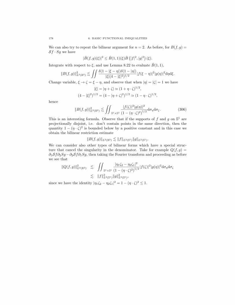
178 6. BASIC FUNCTIONAL INEQUALITIES
We can also try to repeat the bilinear argument for n = 2. As before, for B(f, g) =Sf · Sg we have
|B(f, g)(ξ)|2 ≤ B(1, 1)(ξ)B(|f |2, |g|2
)(ξ).
Integrate with respect to ξ, and use Lemma 8.22 to evaluate B(1, 1),
‖B(f, g)‖2L2(R2) .∫∫
δ(1− |ξ − η|)δ(1− |η|)|ξ|(4− |ξ|2)1/2
|f(ξ − η)|2|g(η)|2dηdξ.
Change variable, ξ → ζ = ξ − η, and observe that when |η| = |ζ| = 1 we have
|ξ| = |η + ζ| ' (1 + η · ζ)1/2,
(4− |ξ|2)1/2 = (4− |η + ζ|2)1/2 ' (1− η · ζ)1/2,
hence
‖B(f, g)‖2L2(R2) .∫∫
S1×S1
|f(ζ)|2|g(η)|2
(1− (η · ζ)2)1/2
dσηdσζ . (306)
This is an interesting formula. Observe that if the supports of f and g on S1 areprojectionally disjoint, i.e. don’t contain points in the same direction, then thequantity 1 − (η · ζ)2 is bounded below by a positive constant and in this case weobtain the bilinear restriction estimate
‖B(f, g)‖L2(R2) . ‖f‖L2(S1)‖g‖L2(S1).
We can consider also other types of bilinear forms which have a special struc-ture that cancel the singularity in the denominator. Take for example Q(f, g) =∂1Sf∂2Sg−∂2Sf∂1Sg, then taking the Fourier transform and proceeding as beforewe see that
‖Q(f, g)‖2L2(R2) .∫∫
S1×S1
|η1ζ2 − η2ζ1|2
(1− (η · ζ)2)1/2|f(ζ)|2|g(η)|2dσηdσζ
. ‖f‖2L2(S1)‖g‖2L2(S1),
since we have the identity |η1ζ2 − η2ζ1|2 = 1− (η · ζ)2 ≤ 1.
Part 3
Analysis of the Wave Equation inMinkowski Space

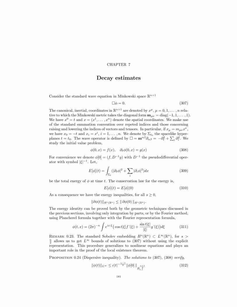
CHAPTER 7
Decay estimates
Consider the standard wave equation in Minkowski space Rn+1
φ = 0. (307)
The canonical, inertial, coordinates in Rn+1 are denoted by xµ, µ = 0, 1, . . . , n rela-tive to which the Minkowski metric takes the diagonal form mµν = diag(−1, 1, . . . , 1).We have x0 = t and x = (x1, . . . , xn) denote the spatial coordinates. We make useof the standard summation convention over repeted indices and those concerningraising and lowering the indices of vectors and tensors. In particular, if xµ = mµνx
ν ,we have x0 = −t and xi = xi, i = 1, . . . , n. We denote by Σt0 the spacelike hyper-planes t = t0. The wave operator is defined by = mαβ∂αβ = −∂2
t +∑i ∂
2i . We
study the initial value problem,
φ(0, x) = f(x), ∂tφ(0, x) = g(x) (308)
For convenience we denote φ[0] = (f,D−1g) with D−1 the pseudodifferential oper-ator with symbol |ξ|−1. Let,
E[φ](t) =
∫Σt
(|∂tφ|2 +∑i
|∂iφ|2)dx (309)
be the total energy of φ at time t. The conservation law for the energy is,
E[φ](t) = E[φ](0) (310)
As a consequence we have the energy inequalities, for all s ≥ 0,
‖∂φ(t)‖Hs(Rn) ≤ ‖ ∂φ(0) ‖Hs(Rn).
The energy identity can be proved both by the geometric techniques discussed inthe previous sections, involving only integration by parts, or by the Fourier method,using Plancherel formula together with the Fourier representation formula,
φ(t, x) = (2π)−n∫eix·ξ
(cos t|ξ|f (ξ) +
sin t|ξ||ξ|
g (ξ))dξ (311)
Remark 0.23. The standard Sobolev embedding Hs(Rn) ⊂ L∞(Rn), for s >n2 allows us to get L∞ bounds of solutions to (307) without using the explicitrepresentation. This procedure generalizes to nonlinear equations and plays animportant role in the proof of the local existence theorem.
Proposition 0.24 (Dispersive inequality). The solutions to (307), (308) verify,
‖φ(t)‖L∞ ≤ c|t|−n−1
2 ‖φ[0] ‖Bn+1
21,1
(312)
181
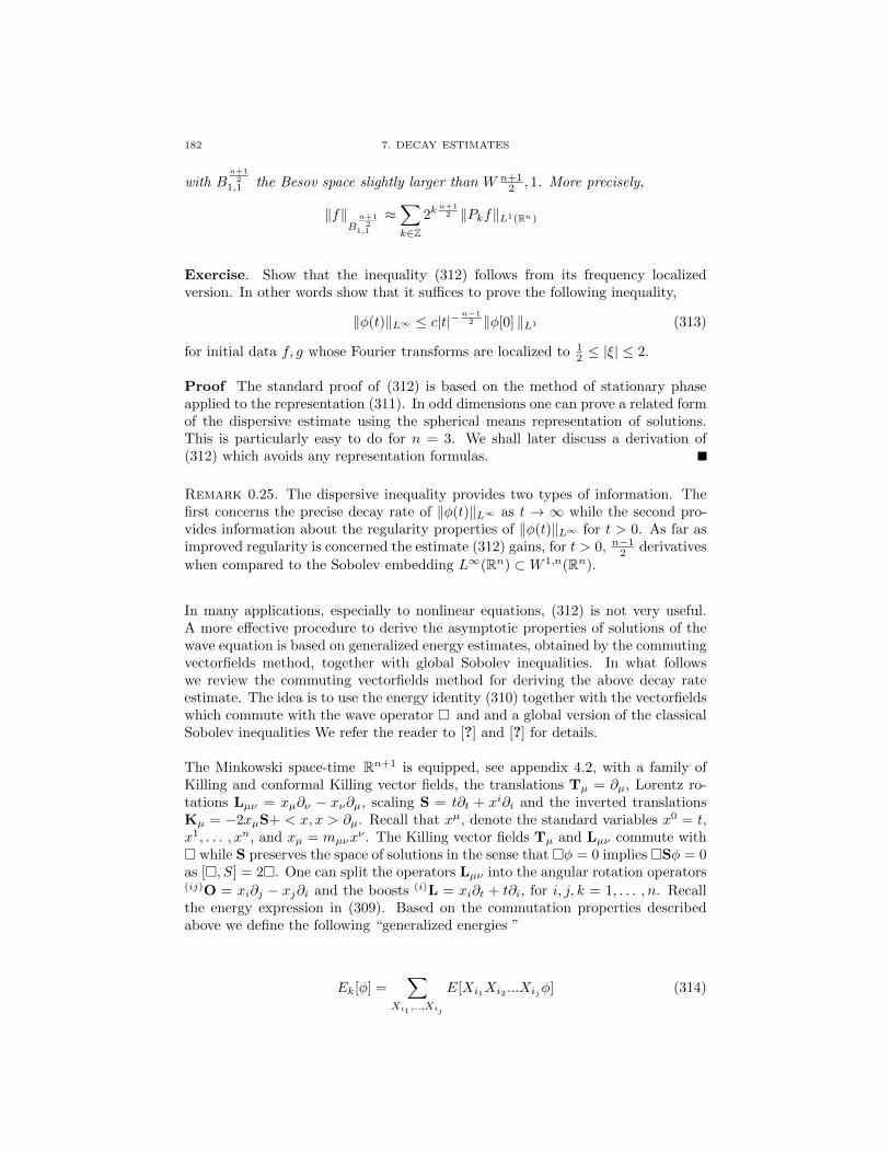
182 7. DECAY ESTIMATES
with Bn+1
21,1 the Besov space slightly larger than W n+1
2 , 1. More precisely,
‖f‖Bn+1
21,1
≈∑k∈Z
2kn+1
2 ‖Pkf‖L1(Rn)
Exercise. Show that the inequality (312) follows from its frequency localizedversion. In other words show that it suffices to prove the following inequality,
‖φ(t)‖L∞ ≤ c|t|−n−1
2 ‖φ[0] ‖L1 (313)
for initial data f, g whose Fourier transforms are localized to 12 ≤ |ξ| ≤ 2.
Proof The standard proof of (312) is based on the method of stationary phaseapplied to the representation (311). In odd dimensions one can prove a related formof the dispersive estimate using the spherical means representation of solutions.This is particularly easy to do for n = 3. We shall later discuss a derivation of(312) which avoids any representation formulas.
Remark 0.25. The dispersive inequality provides two types of information. Thefirst concerns the precise decay rate of ‖φ(t)‖L∞ as t → ∞ while the second pro-vides information about the regularity properties of ‖φ(t)‖L∞ for t > 0. As far asimproved regularity is concerned the estimate (312) gains, for t > 0, n−1
2 derivatives
when compared to the Sobolev embedding L∞(Rn) ⊂W 1,n(Rn).
In many applications, especially to nonlinear equations, (312) is not very useful.A more effective procedure to derive the asymptotic properties of solutions of thewave equation is based on generalized energy estimates, obtained by the commutingvectorfields method, together with global Sobolev inequalities. In what followswe review the commuting vectorfields method for deriving the above decay rateestimate. The idea is to use the energy identity (310) together with the vectorfieldswhich commute with the wave operator and and a global version of the classicalSobolev inequalities We refer the reader to [?] and [?] for details.
The Minkowski space-time Rn+1 is equipped, see appendix 4.2, with a family ofKilling and conformal Killing vector fields, the translations Tµ = ∂µ, Lorentz ro-tations Lµν = xµ∂ν − xν∂µ, scaling S = t∂t + xi∂i and the inverted translationsKµ = −2xµS+ < x, x > ∂µ. Recall that xµ, denote the standard variables x0 = t,x1, . . . , xn, and xµ = mµνx
ν . The Killing vector fields Tµ and Lµν commute with while S preserves the space of solutions in the sense that φ = 0 implies Sφ = 0as [, S] = 2. One can split the operators Lµν into the angular rotation operators(ij)O = xi∂j − xj∂i and the boosts (i)L = xi∂t + t∂i, for i, j, k = 1, . . . , n. Recallthe energy expression in (309). Based on the commutation properties describedabove we define the following “generalized energies ”
Ek[φ] =∑
Xi1 ,..,Xij
E[Xi1Xi2 ...Xijφ] (314)
7. DECAY ESTIMATES 183
with the sum taken over 0 ≤ j ≤ k and over all Killing vector fields T,Lµν as wellas the scaling vector field S. The crucial point of the commuting vectorfield methodis that the quantities Ek, k ≥ 1 are conserved by solutions to (307). Therefore, if,∑
0≤k≤s
∫(1 + |x|)2k
(|∇k+1f(x)|2 + |∇kg(x)|2
)dx ≤ Cs <∞ (315)
then for all t, Es[φ](t) ≤ Cs. The desired decay estimates of solutions to (307) cannow be derived from the following global version of the Sobolev inequalities ( see[?], [?]):
Theorem 0.26 (Global Sobolev). Let φ be an arbitrary function in Rn+1 such thatEs[φ] is finite for some integer s > n
2 . Then,
|∂φ(t, x)| . (1 + t+ |x|)−n−1
2 (1 + |t− |x||)− 12 sup
0≤t′≤tEs[φ](t′)
(316)
for all t > 0. Therefore if the data f, g in (307) satisfy 315, with s > n2 , then for
all t ≥ 0,
|∂φ(t, x)| . 1
(1 + t+ |x|)n−12 (1 + |t− |x||) 1
2
(317)
Remark 0.27. Clearly this estimate, whose proof is purely geometric1, implies thedecay properties given by the dispersive inequality (312). In fact it provides moreinformation outside the wave zone |x| ∼ t which fit very well with the expectedpropagation properties of the linear equation φ = 0. On the other hand, as (316)is really a global version of the Sobolev inequality, it seems that the estimates ofthe Proposition 0.26 have no bearing on the improved regularity features of (312).This is however not quite true as we shall see, later.
Proof We only sketch the main ideas of the proof below. Consider the canonicalnull pair L± = ∂t ± ∂r,, an associated null frame e1, . . . en−1, en = L−, en+1 = L+
as well as the angular vectorfields, Ai = ∂i − xir ∂r. Clearly,∑
i
|Aiφ| . |∇/ φ| .∑i
|Aiφ|.
where |∇/ φ|2 =∑n−1i=1 |ei(φ)|2. Also,
|∂rφ|+∑i
|Aiφ| . |∇φ| . |∂rφ|+∑i
|Aiφ|
We can also easily check the following simple algebraic identities,
1
2
((t+ r)L+ + (t− r)L−
)= S
1
2
((t+ r)L+ − (t− r)L−
)=
∑i
xi|x|
Li
tAi = Li −xi|x|∑j
xj|x|Lj
tOij = xiLj − xjLi
1 In particular it does not require any explicit representation of solutions
184 7. DECAY ESTIMATES
From the first two identities we easily derive,
|L+φ(t, x)| . 1
t|Γφ(t, x)|
|L−φ(t, x)| . 1∣∣t− |x|∣∣ |Γφ(t, x)| (318)
with |Γφ| = |Sφ|+ |Lφ|.
|∇/ φ(t, x)| . 1
t|Γφ(t, x)|. (319)
Clearly, we also have,
|∂φ(t, x)| . 1∣∣t− |x|∣∣ |Γφ(t, x)|
or, more generally,
|∂Nφ(t, x)| . 1∣∣t− |x|∣∣N |ΓNφ(t, x)| (320)
where |ΓNφ| =∑|Γ1 . . .ΓNφ| with Γ1, . . . ,ΓN any of the vectorfields S,L1, . . . Ln.
Combining the above inequalities with the definition of our norms we derive
t‖E+φ(t)‖L2 . ‖Γφ(t)‖L2(Rn)
t‖∇/ φ(t)‖L2 . ‖Γφ(t)‖L2(Rn)
‖uE−φ(t)‖L2 . ‖Γφ(t)‖L2(Rn)
where u = |t− |x|| It remains to derive sup-norm estimates from the L2 estimatesabove.
Proposition 0.28. Let φ = 0 with initial data verifying the assumptions above.Then, for all t ≥ 0, s > n
2 ,
‖φ(t)‖L∞ .(1
t
)n−12 ‖Γsφ(t)‖L2(Rn) (321)
‖(1 + |u|)k∂kφ(t)‖L∞ .(1
t
)n−12 ‖Γsφ(t)‖L2(Rn) (322)
Also,
‖E+φ(t)‖L∞ .(1
t
)n+12 ‖Γs+1φ(t)‖L2(Rn)
‖∇/ φ(t)‖L∞ .(1
t
)n+12 ‖Γs+1φ(t)‖L2(Rn)
‖(1 + |u|)E−φ(t)‖L∞ .(1
t
)n−12 ‖Γs+1φ(t)‖L2(Rn)
7. DECAY ESTIMATES 185
The proof is based on the following Lemma
Lemma 0.29. Let u(x) be a smooth, compactly supported function on Rn, n ≥ 2.We have,
|u(x)| ≤ C 1
|x|n−1
(‖∂ru‖L1 + ‖(r∇/ )n−1∂ru‖L1
)(323)
Proposition 0.30 ( see[?]). The commuting vectorfields method implies the dis-persive inequality (312).
Proof Without loss of generality we may assume that ∂tφ = g = 0 and that theFourier transform of f = φ(0) is supported in the shell λ
2 ≤ |ξ| ≤ 2λ for some
λ ∈ 2N. By a simple scaling argument we may in fact assume λ = 1. For suchinitial conditions, with Fourier supports restricted to 1/2 ≤ |ξ| ≤ 2, it suffices toprove,
‖φ(t)‖L∞ . (1 + |t|)−n−1
2 ‖f‖L1(Rn)
Since φ, the Fourier transform of φ relative to the space variables x, is also supportedin the same shell it suffices to prove the estimates for ∇φ instead of φ.
Next we cover Rn by an union of discs DI centered at points I ∈ Zn with integercoordinates such that each DI intersects at most a finite number cn of discs DJ
with cn depending only on the dimension n. Consider a smooth partition of unity(χI)I∈Zn with suppχI ⊂ DI and each χI positive. Clearly we can arrange to have,for all k, ∑
I∈Zn|∇kχI(x)| ≤ Ck,n (324)
uniformly in x ∈ Rn, with a constant Cn,k depending only on n and k. Nowset, fI = χI · f , and φI the corresponding solution to (307) with data φI(0) =fI , ∂tφI(0) = 0. Clearly f =
∑I fI , φ =
∑I φI . It suffices to prove that for all I,
‖∇kφI(t)‖L∞ . (1 + t)−n−1
2
n+k+1∑j=0
‖DjfI‖L1 (325)
Indeed if (325) holds true we easily infer that,
‖∇kφ(t)‖L∞ ≤∑I
‖∇kφI(t)‖L∞ . (1 + t)−n−1
2
n+k+1∑j=0
∑I
‖DjfI‖L1
186 7. DECAY ESTIMATES
In view of (324) we have,∑I
‖DjfI‖L1 =∑I
‖Dj(χIf)‖L1 .∑I
∑0≤i≤j
∫Rn|DiχI(x)||Dj−if(x)|dx
=∑
0≤i≤j
∫Rn
( ∑I
|DiχI(x)| )∣∣Dj−if(x)|dx
.∑
0≤i≤j
ci,n‖Dj−if‖L1(Rn) . ‖f‖L1(Rn)
Hence,
‖∇kφ(t)‖L∞ . (1 + t)−n−1
2 ‖f‖L1(Rn)
as desired.
It therefore remains to check (325). Without loss of generality, by performing aspace translation, we may assume that I = 0. Applying the proposition 0.26 toψ = ∇φ0 we derive, for s∗ the first integer strictly larger than n
2 ,
‖ψ(t)‖L∞ ≤ c(1 + t)−n−1
2 Es∗ [φ0](t)
≤ c(1 + t)−n−1
2 Es∗ [φ0](0).
Since the support of φ0 is included in in the ball of radius 1 centered at the originwe have,
Es∗ [φ0](0) ≤ Cns∗+1∑j=0
‖Djf0‖L2 .
Finally, according to the standard Sobolev inequality in Rn, ‖f‖L2 ≤ c‖∇n2 f‖L1 ,
we conclude with,
‖ψ(t)‖L∞ ≤ c(1 + t)−n−1
2
n+2∑j=0
‖Djf0‖L1
as desired.
CHAPTER 8
Strichartz Inequalities
Strichartz inequalities are an important tool in the study of linear and nonlinearwave equations. They are intimately tied to restriction theorems. In this chapterwe shall only consider the case of the standard linear wave equation. Similar in-equalities hold true however for linear dispersive equations such as the Schrodinger,linear KdV etc.
0.30.1. Homogeneous wave equation. Consider solutions u = u(t, x), t ∈ R, x ∈Rn to the equation
u = F, (326)
u(0, x) = f(x), ∂tu(0, x) = g(x), (327)
with the wave operator 2 = −∂2t u + ∆. Clearly, a solution to eqrefeq:genwave
can be written as a superposition between a solution to the homogeneous waveequation,
2u = 0, (328)
verifying the initial condition (327) at time t = 0, and a solution to the purelyinhomogeneous wave equation
2u = F, (329)
with zero initial data
u(0, x) = 0, ∂tu(x, 0) = 0.
We denote by W (t)h the fundamental solution of the homogeneous problem (328),i.e. u(t, x) =
(W (t)h
)(x) is the unique solution of (328) which verifies the initial
conditions
u(0, x) = 0, ∂tu(0, x) = h(x)
By Duhamel’s principle any solution of the inhomogeneous equation can itself bewritten as a superposition of solutions to the homogeneous equation according tothe formula,
u(t) =
∫ t
0
W (t− t′)F (t′)dt′, (330)
Before stating the main result of this section we make the following definition.
187
188 8. STRICHARTZ INEQUALITIES
Definition 0.31. We say that the pair of real numbers (q, r) is an admissible wavepair if they satisfy the conditions
q ≥ 2,
2
q≤ (n− 1)
(1
2− 1
r
),
(q, r, n) 6= (2,∞, 3).
We are now ready to state the following.
Theorem 0.32. Suppose that n ≥ 2 and (q, r) is a wave admissible pair 1 withr <∞.
(1) Assume the dimensional condition, 1q + n
r = n2 − γ. Then, if u verifies the
homogeneous equation (328) with initial conditions (327),
‖u‖LqtLrx + ‖u‖L∞t Hγx + ‖∂tu‖L∞t Hγ−1x
. ‖f‖Hγ + ‖g‖Hγ−1 (331)
(2) Assume the dimensional condition,2 1q + n
r = n2 − γ = 1
q′ + nr′ − 2, with q′
dual to q and r′ dual to r. Then, if u verifies the purely inhomogeneousproblem (0.30.1) with zero initial conditions, then on a finite time interval[0, T ]:
‖u‖Lq([0,T ];Lr) + ‖u‖C([0,T ];Hγ) + ‖∂tu‖C([0,T ];Hγ−1) . ‖F‖Lq′ ([0,T ];Lr′ )(332)
(3) We also have the following more general version of (332) for admissiblepairs (q1, r1), (q2, r2) with r1, r2 <∞ verifying the dimensional condition,
1
q1+n
r1=n
2− γ =
1
q′2+n
r′2− 2
Then,
‖u‖Lq1 ([0,T ];Lr1 ) + ‖u‖C([0,T ];Hγ) + ‖∂tu‖C([0,T ];Hγ−1) . ‖F‖Lq′2 ([0,T ];Lr
′2 )
(333)
Remark 0.33. For n ≥ 4, the region of admissable exponents corresponds to aquadrilateral OEPQ in the plane (1/q, 1/r) with vertices O = (1/∞, 1/∞), E =(1/∞, 1/2), P = (1/2, n−3
2(n−1) ) and Q = (1/2, 1/∞). When n = 3 the point P
coincides with Q and the region reduces to the triangle OEQ. When n = 2 we havea smaller triangle OEQ2 where Q2 = (1/4, 1/∞).
For n = 3, the boundary of the triangular region is allowed except for the endpointP . For n ≥ 4, the boundary of the quadrilateral region is entirely allowed, as wewill note below.
The interesting cases are the ones on the segment EP and the ones on PQ closeto P , since all the others can be deduced from these using Sobolev embeddings.The point E corresponds to the energy estimates. There are counterexamples that
1The case when r =∞ can also be included provided that we modify the spaces on the left
of the estimates below to appropriate Besov spaces.2Thus, in fact, γ = 1/2.
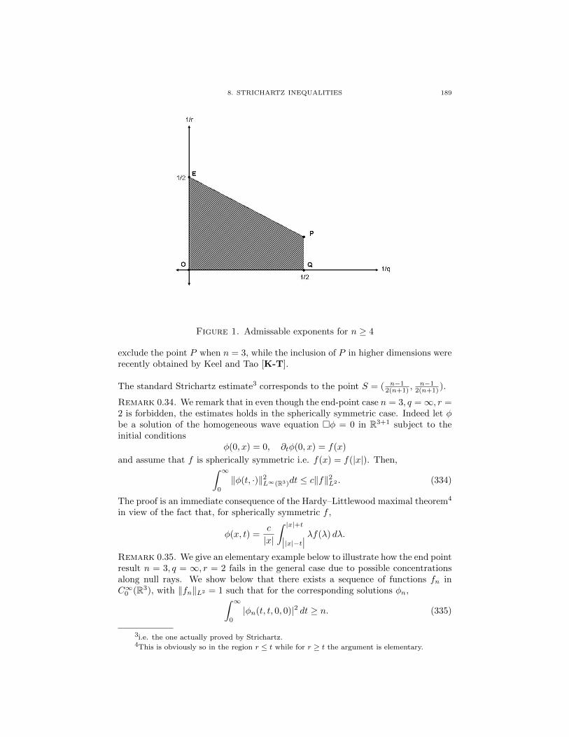
8. STRICHARTZ INEQUALITIES 189
Figure 1. Admissable exponents for n ≥ 4
exclude the point P when n = 3, while the inclusion of P in higher dimensions wererecently obtained by Keel and Tao [K-T].
The standard Strichartz estimate3 corresponds to the point S = ( n−12(n+1) ,
n−12(n+1) ).
Remark 0.34. We remark that in even though the end-point case n = 3, q =∞, r =2 is forbidden, the estimates holds in the spherically symmetric case. Indeed let φbe a solution of the homogeneous wave equation φ = 0 in R3+1 subject to theinitial conditions
φ(0, x) = 0, ∂tφ(0, x) = f(x)
and assume that f is spherically symmetric i.e. f(x) = f(|x|). Then,∫ ∞0
‖φ(t, ·)‖2L∞(R3)dt ≤ c‖f‖2L2 . (334)
The proof is an immediate consequence of the Hardy–Littlewood maximal theorem4
in view of the fact that, for spherically symmetric f ,
φ(x, t) =c
|x|
∫ |x|+t∣∣|x|−t∣∣ λf(λ) dλ.
Remark 0.35. We give an elementary example below to illustrate how the end pointresult n = 3, q = ∞, r = 2 fails in the general case due to possible concentrationsalong null rays. We show below that there exists a sequence of functions fn inC∞0 (R3), with ‖fn‖L2 = 1 such that for the corresponding solutions φn,∫ ∞
0
|φn(t, t, 0, 0)|2 dt ≥ n. (335)
3i.e. the one actually proved by Strichartz.4This is obviously so in the region r ≤ t while for r ≥ t the argument is elementary.
190 8. STRICHARTZ INEQUALITIES
assume by contradiction that in fact, J :=∫∞
0φ(t, t, 0, 0)ϕ(t) dt < C for all f ∈
C∞0 (R3) with ‖f‖L2 = 1 and some ϕ ∈ S(R), ϕ 6≡ 0. In view of the formula (seesection on the fundamental solution of in R3+1),
φ(t, x) = (4π)−1t
∫|ξ|=1
f(x+ tξ) dξ
we find that,
J = (4π)−1
∫R3
|y|−1f1(y1 + |y|, y2, y3)ϕ(|y|) dy
or, changing the variables z = y + (|y|, 0, 0)
J = (4π)−1
∫z1>0
1
z1f(z)ϕ
( |z|22z1
)dz < c.
Since f is an arbitrary C∞0 (R3) function, ‖f‖L2 = 1, we must have that,
z → 1
z1ϕ( |z|2
2z1
)is in L2(R3
+) which is false whenever ϕ 6≡ 0. In fact,∫R3
+
1
z21
ϕ2( |z|2
2z1
)dz =
∫R3
1
(y1 + |y|)|y|ϕ2(|y|)dy = 2π
∫ ∞0
ϕ2(λ)
∫ π
0
sin θ
1 + cos θdθ
diverges logarithmically if ϕ 6≡ 0.
0.36. Fourier representation of solutions. We can solve the homogeneousproblem (328) by the Fourier method. To recall, If we apply the Fourier transformwith respect to the space variables, the initial value problem (328), (327) becomesa Cauchy problem for an ordinary differential equation:
∂2t u+ |ξ|2u = 0, u(0, ξ) = f(ξ), ∂tu(0, ξ) = g(ξ),
which can be solved explicitly:
u(t, ξ) = cos (t|ξ|) f(ξ) + sin (t|ξ|) g(ξ)
|ξ|(336)
Thus the fundamental solution W (t)h, defined above, takes the form,
W (t)h(x) =
∫Rneix·ξ
sin(t|ξ|)|ξ|
h(ξ)dξ. (337)
By Duhamel principle, see (330), the general solution of the inhomogeneou equationu = F can be expressed in the form,
u(t) = ∂tW (t)f +W (t)g +
∫ t
0
W (t− s)F (s)ds. (338)
let D = (−∆)1/2 be the operator whose symbol in Fourier space is given by |ξ|.Observe that,
(DW (t))f(x) = (W (t)Df)(x) =
∫Rneix·ξ sin t|ξ|)f(ξ)dξ.
Since sin t|ξ| and cos t|ξ| are bounded the operators ∂tW (t) andDW (t) mapHs(Rn)in itself. In particular, solutions u of (328), (327) preserves the (Sobolev) regularity
8. STRICHARTZ INEQUALITIES 191
of the initial data f and g. More precisely, If f,D−1g ∈ Hs for some s ∈ R, thenu(t), D−1∂tu(t) ∈ Hs uniformly for t ∈ R. We can also write,
‖u‖L∞t Hγx + ‖∂tu‖L∞t Hγ−1x
. ‖f‖Hγ + ‖g‖Hγ−1
which provides the easy part of estimate5 (331). Therefore to prove (331) it sufficesto prove,
‖u‖LqtLrx . ‖f‖Hγ + ‖g‖Hγ−1 (339)
for and wave admissible pair (q, r).
We also remark that,
∂tW (t)h(x) =
∫Rneix·ξ cos(t|ξ|)h(ξ)dξ
and,
D−1W (t)h(x) =
∫Rneix·ξ
cos(t|ξ|)|ξ|
h(ξ)dξ
We can rewrite (336) as
u(t, ξ) = eit|ξ|f+(ξ) + e−it|ξ|f−(ξ),
where f± = 12
(f ±D−1g
). It follows that u = u+ + u− where
u± =
∫ei(x·ξ±t|ξ|)f±(ξ)dξ
Observe that to prove (339) it suffices to prove,
‖u+‖LqtLrx . ‖f+‖Hγ (340)
and a similar estimate for f−.
0.37. Energy estimates. We will derive a simple L2 estimate for generalsolutions of u = F by integration by parts. It all follows from the simple algebraicidentity:
− 1
2∂t(|∂tu|2 + |∇u|2) + ∂i(∂tu∂iu) = ∂tu · F (341)
where |∇u|2 =∑ni=1(∂iu)2 and ∂i = ∂xi . Integrating with respect to x, and
assuming that u and its derivatives vanish6 at infinity we derive,
∂t
∫Rn
((∂tu)2 + |∇u|2
)dx = 2
∫Rn∂tu · Fdx
Thus integrating in t,
‖∂tu(t)‖2L2 + ‖∇u(t)‖2L2 ≤ ‖∂tu(0)‖2L2 + ‖∇u(0)‖2L2 + 2
∫ t
0
∫Rn∂tu · Fdxds
5Another derivation, based on energy identities, is given in the next subsection.6This can easily be justified by the finite propagation speed property of solutions to the wave
equation
192 8. STRICHARTZ INEQUALITIES
which we rewrite, with |∂u|2 = |∂tu|2 + |∇u|2,
‖∂u(t)‖2L2 = ‖∂u(0)‖2L2 + 2
∫ t
0
∫Rn∂tu · Fdxds. (342)
In particular, applying Holder,
‖∂u(t)‖2L2 ≤ ‖∂u(0)‖2L2 + 2
∫ t
0
‖∂tu(s)‖L2‖F (s)‖L2ds
from which we derive the inhomogeneous energy estimate,
supt∈[0,T ]
‖∂u(t)‖L2 . ‖∂u(0)‖L2 +
∫ T
0
‖F (s)‖L2ds (343)
Now let Ds be the operator Ds = (−∆)s/2 whose symbol in Fourier space is givenby |ξ|s. Since Ds commutes with we easily derive,
‖∂Dsu(t)‖2L2 = ‖∂Dsu(0)‖2L2 + 2
∫Rn∂tD
su ·DsFdx
We can write, using Plancherel with respect to the x variables,∫Rn∂tD
su ·DsFdx =
∫Rn∂tD
2su · Fdx,
Therefore, by Holder, in the slab DT = [0, T ]× Rn,
supt∈[0,T ]
‖∂Dsu(t)‖2L2 ≤ ‖∂Dsu(0)‖2L2 + 2‖D2s∂tu‖LqtLrx(DT )‖F‖Lq′t Lr′x (DT )
Choosing s = −1 we infer that,
supt∈[0,T ]
‖∂D−1/2u(t)‖2L2 ≤ ‖∂D−1/2u(0)‖2L2 + 2‖D−1∂tu‖LqtLrx(DT )‖F‖Lq′t Lr′x (DT )
We apply this energy estimate to solution of the inhomogeneous problem (0.30.1)with zero initial conditions. We also assume that the dimensional condition 1
q + nr =
n2 − γ = 1
q′ + nr′ − 2 is verified. That implies γ = 1
2 . We thus have,
supt∈[0,T ]
‖∂D−1/2u(t)‖2L2 ≤ 2‖D−1∂tu‖LqtLrx(DT )‖F‖Lq′t Lr′x (DT )
Assume for a moment that we can prove the estimate,
‖D−1∂tu‖LqtLrx(DT ) . ‖F‖Lq′t Lr′x (DT )(344)
Then,
supt∈[0,T ]
‖∂D−1/2u(t)‖L2 . ‖F‖Lq′t L
r′x (DT )
which is equivalent to,
supt∈[0,T ]
(‖u(t)‖Hγ) + ‖∂tu‖Hγ−1)
). ‖F‖Lq′ ([0,T ];Lr′ )
thus proving half of estimate (332). Therefore the inhomogeneous estimate (332)reduces to proving,
‖u‖Lq([0,T ];Lr) + ‖D−1∂tu‖Lq([0,T ];Lr) . ‖F‖Lq′ ([0,T ];Lr′ ) (345)
8. STRICHARTZ INEQUALITIES 193
0.38. Homogenous Case. In this section we prove estimate (340) and thuscomplete the proof for the homogeneous Strichartz estimate of theorem 0.32. Usingthe space-time Fourier transform, i.e. Fourier transform with respect to both t andx,
u+(τ, ξ) = δ(τ − |ξ|)f+(ξ), u−(τ, ξ) = −δ(τ + |ξ|)f−(ξ), (346)
These are the components of u living on the forward null cone C+ = τ = |ξ| andon the backward null cone C− = τ = −|ξ|, respectively. Thus we can interpret(340) from the point of view of a restriction theorem for the half light cones C+ or
C−. We next show that it suffices to prove (340) for the case when f+ is includedin fixed dyadic piece. More precisely, dropping the label + it suffices to show that,
‖u+k ‖LqtLrx . 2kγ‖f+
k ‖L2 (347)
where u+ =∑k∈2Z u
+k , u+
k = Pku+, f+
k = Pkf+ and Pk the standard LP projec-
tions with respect to the spatial variables x.
To show that (348) implies (340) is highly nontrivial7 as we need to rely on corollary6.15 adapted to the mixed norms LqtL
rx with both q and r larger than 2. Thus,
‖u+‖2LqtLrx .∑k∈Z‖u+
k ‖2LqtL
rx.∑k∈Z
22kγ‖f+k ‖
2L2 . ‖f+‖Hγ
Finally we observe, using a simple scaling argument, that (348) follows from,
‖u+0 ‖LqtLrx . ‖f+
0 ‖L2 (348)
We now define the truncated cone operator C to be the operator
Cf(t, x) =
∫eit|ξ|eix·ξχ(ξ)f(ξ)dξ, (349)
where χ is a cut-off function supported in 1.2 ≤ |ξ| ≤ 2, such as the one used inthe definition of the LP projections, see (214). The operator C can be viewed asthe adjoint of the restriction of the Fourier transform to a truncated cone,
C∗F (ξ) = χ(ξ) F (|ξ|, ξ)Estimate (348) is an immediate consequence of the following theorem.
Theorem 0.39. Let (q, r), (q1, r1), (q2, r2) be admissable pairs of exponents. Thenwe have the estimates
‖Cf‖LqtLrx . ‖f‖L2 , (350)
and also
‖CC∗F‖Lq1t Lr1x . ‖F‖Lq′2t Lr′2x
. (351)
Composing C with C∗ we derive,
CC∗F (t, x) '∫ei[(t−s)|ξ|+(x−y)·ξ]|β(ξ)|2F (s, y)dsdydξ,
7Without using corollary 6.15 we would only derive a weaker estimate with the Besov normBγ2,1 replacing Hγ norm on the right.
194 8. STRICHARTZ INEQUALITIES
which can be rewritten as the convolution
CC∗F (t, ·) =
∫U(t− s)F (s, ·)ds, (352)
with the evolution operator
U(t)f(x) =
∫ei(t|ξ|+x·ξ)|χ(ξ)|2f(ξ)dξ. (353)
(Observe that U is essentially the same operator as C !) By the TT ∗ principle, weknow that the estimate (350) is equivalent to the following estimate for CC∗,
‖CC∗F‖LqtLrx . ‖F‖Lq′t Lr′x . (354)
which is also equivalent to the polarized form (351). Thus, to prove the theorem itsuffices to prove (354). As in the second proof of the restriction theorem presentedin the previous section to prove (354) we need to prove the following properties forthe evolution operators U(t).
Proposition 0.40. Let χ(ξ) be a fixed C∞0 (Rn) function supported in 1/2 ≤ |ξ| ≤ 2and,
U(t)f(x) =
∫ei(t|ξ|+x·ξ)χ(ξ)f(ξ)dξ. (355)
Then,
‖U(t)f‖L2 . C‖f‖L2 (356)
‖U(t)f‖L∞ . (1 + |t|)−n−1
2 ‖f‖L1 (357)
from which, interpolating, for all 2 ≤ r ≤ ∞,
‖U(t)f‖Lr . (1 + |t|)−n−1
2 (1− 2r )‖f‖Lr′ (358)
Moreover, if in addition, χ = χµ is supported in a cube of size µ, then (357) canbe strengthened to
‖U(t)f‖L∞ . µ(1 + |t|)−n−1
2 ‖f‖L1 (359)
Proof We prove directly the stronger version (359). We only need to check (??).We write,
U(t)f = Kt ∗ f, Kt(x) =
∫ei(x·ξ+t|ξ|)χµ(ξ)dξ
It suffices to show that,
|Kt(x)| . µ 1
(1 + |t|+ |x|)In the regions |x| < |t|/2 and |x| ≥ 2|t| we integrate by parts k times with respect to
the operator L = −i∑j
xj+tξj|ξ
|x+t ξ|ξ| |2∂ξj , such that L(ei(x·ξ+t|ξ|)) = ei(x·ξ+t|ξ|). We also
make use of the straightforward estimate, |∂αξ χµ(ξ)| . µ−|α| to derive, |Kt(x)| .(1 + |t|)−kµn−k or, choosing k = n−1
2 ,
|Kt(x)| . (1 + |t|)−n−1
2 µn+1
2 .
8. STRICHARTZ INEQUALITIES 195
On the other hand, in the region |t| ≈ |x|, we write, with β(|ξ|) vanishing on thesupport of hµ,
Kt(x) =
∫ 1+2µ
1−2µ
eitλχ(λ)
∫|ξ|=λ
eix·ξhµ(ξ)dσ(ξ)
We now need to rely on the following estimate,
sup1/2≤λ≤2
|∫|ξ|=λ
eix·ξh(ξ)dσ(ξ)| . (1 + |x|)−n−1
2 (360)
which follows easily from the decay of the Fourier transform of measures supportedon Sn−1 discussed in the previous section, see lemma 8.8. Therefore, for |t| ∼ |x|,
|Kt(x)| . µ(1 + |x|)−n−1
2 . µ(1 + |t|)−n−1
2
as desired.
We are now ready to prove (354) by following the same argument as in the secondproof of the restriction theorem. Indeed, in view of (352) and (358) we derive,
‖CC∗F‖Lrx(t) .∫ +∞
−∞(1 + |t− s|)−γ(r)‖F (s)‖Lr′x ds (361)
where γ(r) = −n−12 (1 − 2
r ). We are now precisely in the same situation as in thesecond proof of the restriction theorem, see the argument following formula (300).If 0 < γ(r) < 1 we can apply the Hardy-Littlewood-Sobolev inequality to obtain
‖CC∗F‖LqtLrx . ‖F‖Lq′t Lr′x ,
when −γ(r) + 1 + 1/q = 1/q′, hence γ(r) = 2/q. This proves (348), and thustheorem 0.39, in the case 0 < γ(r) = 2/q < 1. If q = 2 and γ(r) > 1 we have from(361),
‖CC∗F‖L2tL
rx. ‖F‖L2
tLr′x,
by an application of the standard Hausdorff-Young inequality.
Finally, if 2/q < 1 and γ(r) > 2/q the result follows from the case γ(r) = 2/q usingSobolev inequalities. Due to the fact that one of the principal curvatures of thelight cone vanishes, the Strichartz estimates for the wave equation is not as strongas it could be. Using the improved dispersive estimate (359) we can however derivea stronger statement ,which is very useful in applications.
Proposition 0.41. Let 0 < µ < 1. Let f be an L2 function with Fourier transformsupported in a cube of size µ at a distance 1 from the origin. Let (q, r) be anadmissable pair of exponents for the Strichartz estimates. Then
‖Cf‖LqtLrx . µ( 1
2−1r )‖f‖L2 . (362)
The proof is based on the improved dispersive estimate (359). Interpolating it with(356) we derive,
‖U(t)f‖Lr . µ1− 2r (1 + |t|)−
n−12 (1− 2
r )‖f‖Lr′The proof the continues exactly as above to derive,
‖CC∗F‖LqtLrx . µ1− 2
r ‖F‖Lq′t L
r′x,
196 8. STRICHARTZ INEQUALITIES
and therefore, by the TT ∗ argument, ‖Cf‖LqtLrx . µ( 12−
1r )‖f‖L2 , as desired. As a
straightforward corollary to the proposition we derive:
Theorem 0.42. Consider a general solution of u = 0 with data f, g supported, inFourier space, on a cube of size µ situated in a dyadic shell of size λ, with λ muchlarger than µ, say λ ≥ 8µ. Then,
‖u‖LqtLrx . µ1− 2
r
(‖f‖Hγ + ‖f‖Hγ−1
)(363)
Proof The proof follows easily by a scaling argument from the proposition above.
Finally we state below another result, which follows easily from the decay estimate(357).
Theorem 0.43. Let u be a free wave, i.e. solution of the homogeneous equationu = 0, with initial data (f, g). Then,
‖u(t)‖L∞ . |t|−n−1
2
∑λ∈2Z
(λn+1
2 ‖fλ‖L1 + λn−1
2 ‖gλ‖L1
)= |t|−
n−12
(‖f‖
Bn+1/21,1
+ ‖g‖Bn−1/21,1
).
The uniform decay rate |t|−n−12 , for large t, plays a very important role in the study
of nonlinear perturbations of the standard wave equation.
0.44. Inhomogeneous Strichartz estimates. We have already reduced theinhomogeneous Strichartz estimate (332) of theorem 0.32 to estimate (345). Pro-ceeding as in the case of the homogeneous estimates we can now reduce (345) tothe case when the spatial Fourier transform of F is supported in the unit dyadicring 1/2 ≤ |ξ| ≤ 2. Moreover, decomposing u as before in the ± parts it suffices toprove the estimates separately for u+ and u−. Therefore we need to prove,
‖u+|Lq([0,T ];Lr) + ‖D−1∂tu+‖Lq([0,T ];Lr) . ‖F‖Lq′ ([0,T ];Lr′ ) (364)
We have,
u+(t, ·) =
∫ t
0
U(t− s)F (s, ·)ds
D−1∂tu+(t, ·) =
∫ t
0
∂tD−1U(t− s)F (s, ·)ds
Since, in view of the dyadic restriction, ∂tD−1U(t) ∼ U(t) it suffices to prove
the estimate for ‖u+|Lq([0,T ];Lr). Clearly, u+ differs from CC∗F in (352) only bythe restriction of the interval of integration to [0, t]. In view of this fact we writeu+ = (CC∗)RF . We are thus led to the following theorem, from which (364) andthus (332).
Theorem 0.45. Let U(t) defined as in (355) and let
(CC∗)RF (t, ·) =
∫ t
0
U(t− s)F (s, ·)ds
8. STRICHARTZ INEQUALITIES 197
Then, for all admissible pairs (q1, r1), (q2, r2),
‖(CC∗)RF‖Lq1t Lr1x ([0,T ]×Rn) . ‖F‖Lq′2t L
r′2x ([0,T ]×Rn)
(365)
Proof The proof is straightforward in the case (q1, r1) = (q2, r2) = (q, r). Indeedin this case we can simply repeat the proof of estimate (354) and just take intoaccount the limits of integration. We have also treated the case when q1 = ∞,r1 = 2, see the subsection on energy estimates. The other non-diagonal case casesare a little more difficult and will be treated in the more general abstract settingdiscuss later in this section. The proof we have given covers however the mostinteresting case of estimate (332). We have thus given complete proofs for the firsttwo parts of theorem 0.32
0.46. Necessity of the admissibility conditions. To understand what isthe optimal range of exponents q and r we consider the analog of the Knapp coun-terexample in the context of the truncated cone operator C defined in (349).
For some small δ > 0, let
D = ξ ∈ Rn : |ξ1 − 1| < 1/2, |ξ′| < δ ,and consider f = χD. We have
Cf(t, x) = ei(t+x1)
∫D
ei[t(|ξ|−ξ1)+(t+x1)(ξ1−1)+x′·ξ′]dξ,
and observe that
|ξ| − ξ1 =|ξ′|2
|ξ|+ ξ1. δ2.
We can then choose a region of space-time R defined by
|t| . δ−2, |t+ x1| . 1, |x′| . δ−1,
such that, when (t, x) ∈ R and ξ ∈ D, then the oscillatory factor inside the lastintegral can be treated as a constant. Hence, |Cf(t, x)| & |D| for (t, x) ∈ R and wehave
‖Cf‖LqtLrx‖f‖L2
&|D|‖χR‖LqtLrx|D|1/2
∼ δn−1
2 −2q−
n−1r .
In the limit δ → 0, an estimate of the form (354) will necessarily imply that q andr satisfy the condition
2
q≤ (n− 1)
(1
2− 1
r
). (366)
The other restriction on the range for q, i.e. q ≥ 2 is a consequence of the invari-ance of the operator CC∗ under time translations. Indeed for translation invariantoperators we have the following general result due to Hormander, [?].
Proposition 0.47. Let T : Lp(Rn) → Lq(Rn) be a (non trivial) linear operatorwhich commutes with translations, in the sense that (Tf) τy = T (f τy), whereτy(x) = x + y, for x, y ∈ Rn. If T is bounded from Lp to Lq then we necessarilyhave q ≥ p.
198 8. STRICHARTZ INEQUALITIES
The proof is based on the following lemma.
Lemma 0.48. Let f ∈ Lp(Rn), then
lim|y|→∞
‖f + f τy‖Lp = 21/p‖f‖Lp .
Proof For every R > 0 consider the decomposition f = gR + hR, where gR(x) =f(x) if |x| < R and 0 if |x| ≥ R, and hR(x) = 0 if |x| < R and f(x) if |x| ≥ R.Then
limR→∞
‖gR‖Lp = ‖f‖Lp , limR→∞
‖hR‖Lp = 0.
For R = |y|/2 we have
f + f τy = gR + gR τy + hR + hR τy.
The functions gR and gR τy have disjoint supports, so that
‖gR + gR τy‖pLp = ‖gR‖pLp + ‖gR τy‖pLp = 2‖gR‖pLp ,
while
lim|y|→∞
‖hR + hR τy‖Lp ≤ lim|y|→∞
2‖hR‖Lp = 0,
hence
lim|y|→∞
‖f + f τy‖Lp = lim|y|→∞
21/p‖gR‖Lp = 21/p‖f‖Lp .
Proof [Proof of Proposition 0.47] Let C > 0 be the optimal constant for theestimate
‖Tf‖Lq ≤ C‖f‖Lp , ∀f ∈ Lp.Then by linearity and the translation invariance,
‖Tf + (Tf) τy‖Lq ≤ C‖f + f τy‖Lp .
When |y| → ∞, applying the lemma we obtain
21/q‖Tf‖Lq ≤ C21/p‖f‖Lp , ∀f ∈ Lp.
The optimality of C implies that 21p−
1q ≥ 1, hence q ≥ p.
The proposition generalizes easily to vector valued Lp spaces and if we considerCC∗ as an operator from Lq
′(R;Lr
′
x ) to Lq(R;Lrx), then we must have q ≥ q′,which is the condition q ≥ 2.
0.49. A general, abstract framework. It turns out that the method ofproving Strichartz estimates described above applies to many other equations, suchas Schrodinger, KdV etc. It thus pays to have a general framework which appliesto all these cases.
Let (X,dµ) be a measure space and H a Hilbert space. Consider a family (U(t))t∈Rof operators U(t) : H → L2(X), which describes the evolution of some system withdata in H. We assume that this evolution satisfies the following two properties:
8. STRICHARTZ INEQUALITIES 199
• for all t ∈ R and f ∈ H we have the energy estimate:
‖U(t)f‖L2(X) . ‖f‖H ; (367)
• for all t 6= s and g ∈ L1(X) we have the dispersive inequality:
‖U(t)U∗(s)g‖L∞(X) . |t− s|−γ0‖g‖L1(X), (368)
for some γ0 > 0.
Interpolating between (367) and (368) we obtain the estimate
‖U(t)U∗(s)g‖Lr(X) . |t− s|−γ(r)‖g‖Lr′ (X), (369)
for r ≥ 2, where
γ(r) = γ0
(1− 2
r
).
Theorem 0.50. If the evolution operator U(t) satisfies (367) and (368), then theestimates
‖U(t)f‖LqtLrX . ‖f‖H , (370)
hold for all q, r ≥ 2 verifing:
2
q= γ(r), (q, r, γ0) 6= (2,∞, 1). (371)
Remark 0.51. This form of the Strichartz inequalities applies to linear dispersiveequations such as Schrodinger.
Proof If we consider the operator T : H → LqtLrX defined by Tf(t, x) = (U(t)f)(x)
then it is easy to verify that the dual of T is the operator T ∗ : Lq′
t Lr′
X → H givenby T ∗F =
∫U∗(s)F (s, ·)ds. By the TT ∗ method, (370) is then equivalent to the
estimate
‖∫U(t)U∗(s)F (s)ds‖LqtLrX . ‖F‖Lq′t Lr′X . (372)
By duality and symmetry considerations, this is in turn equivalent to
|B(F,G)| . ‖F‖Lq′t L
r′X
‖G‖Lq′t L
r′X
, (373)
where B(F,G) is the bilinear form
B(F,G) =
∫∫s<t
〈U∗(t)F (t), U∗(s)G(s)〉dtds. (374)
From the bilinear version of (369) we have that
|B(F,G)| .∫∫‖F (t)‖Lr′‖G(s)‖Lr′
|t− s|γ(r)dsdt. (375)
If γ(r) < 1, we can apply the Hardy-Littlewood-Sobolev inequality and obtain(373). This concludes the proof for the cases q = 2/γ(r) > 2.
The endpoint case, corresponding to γ(r) = 2/q = 1, is allowed when r < ∞. Itsproof will be described in the next section.
200 8. STRICHARTZ INEQUALITIES
Remark 0.52. If we strengthen the dispersive condition (368) to
‖U(t)U∗(s)g‖L∞(X) . (1 + |t− s|)−γ0‖g‖L1(X), (376)
then (375) can be improved to
|B(F,G)| .∫∫‖F (t)‖Lr′‖G(s)‖Lr′
(1 + |t− s|)γ(r)dsdt. (377)
Now we can obtain (373) from Young’s inequality when 2/q = 1/p and (1 +|t|)−γ(r) ∈ Lp(R), i.e. γ(r)p > 1. Hence, (376) allows us to extend the Strichartzestimates (370) in Theorem 0.50 to the range
2
q≤ γ(r), (q, r, γ0) 6= (2,∞, 1). (378)
This case applies to the linear wave equations.
Remark 0.53. We observe that there is a natural scaling associated to the objectsin this abstract formulation. More precisely, the estimates (370) in Theorem 0.50are invariant under the change of scale defined by
U(t)← U(t/λ), U∗(s)← U∗(s/λ), dµ← λγ0dµ, 〈f, g〉H ← λγ0〈f, g〉H .(379)
We can also consider the endpoint case.
q = 2, r =2γ0
γ0 − 1, γ0 > 1.
This, in fact, is more difficult than the previous non-endpoint case, and requiresa two-parameter estimate which is better than the one-parameter family given bythe interpolation (369). This proof is presented in the previously mentioned paperby Keel and Tao, “Endpoint Strichartz Estimates”. We omit it here.
0.54. Inhomogeneous estimates. Saying that an operator T maps the Hilbert
space H into LqtLrX , is equivalent to saying that its dual T ∗ maps Lq
′
t Lr′
X into H,
and is also equivalent to saying that the TT ∗ operator maps Lq′
t Lr′
X into LqtLrX . If
the pair (q, r) is allowed to vary in a set E of admissable exponents, we can viewTT ∗ as a composition of two operators associated with different pairs of exponents.It follows that TT ∗ actually satisfies a larger set of mapping properties, since it
maps Lq′
t Lr′
X into LqtLrX , for any couple of pairs (q, r), (q, r) ∈ E.
The operator Tf(t) = U(t)f defined in the previous subsection can be viewed as thesolution of some homogenous, translation invariant, linear evolution equation. Thesolution of the corresponding inhomogenoues problem, using Duhamel’s principle,would be represented by the retarded operator
RF (t) =
∫s<t
U(t)U∗(s)F (s)ds.
Observe that operator R looks very similar to the TT ∗ operator, which is given by
TT ∗F (t) =
∫U(t)U∗(s)F (s)ds.
8. STRICHARTZ INEQUALITIES 201
The restriction s < t in the definition of R, however, destroys the compositionstructure of TT ∗. Fortunately, all the mapping properties of TT ∗, which we havederived above, can be transfered to R.
Theorem 0.55. The operator R maps Lq′
t Lr′
X into LqtLrX , for any couple of pairs
(q, r), (q, r) for which the Strichartz estimate 370 holds.
Proof First of all observe that in the proof of theorem 0.50 we have actuallyproved the diagonal case (q, r) = (q, r). Indeed, the bilinear form defined in (374)can be written as B(F,G) =
∫∫R(F ) ·Gdxdt and (373) is the dual formulation of
the mapping property for R.
The non diagonal cases with 1q + 1
q < 1 follow from the mapping properties of TT ∗
by using a general argument about integral operators due to Christ and Kiselev(see [] and []) which we summarize in Proposition 0.57 below.
It remains to consider the cases with q = q = 2 and r 6= r, under the assumptionthat the evolution U(t) satisfies the stronger dispersive inequality (376) with γ0 > 1.Since, we have already proved the case r = r, by interpolation it is enough toconsider the extreme case: r = r∗ = 2γ0
γ0−1 , r =∞, and show that
|B(F,G)| . ‖F‖L2tL
r′∗X
‖G‖L2tL
1X.
This estimate follows by decomposing B(F,G) into dyadic pieces, B =∑λ∈2Z Bλ,
where
Bλ(F,G) =
∫∫λ/2≤|t−s|≤2λ
〈U∗(t)F (t), U∗(s)G(s)〉dtds, (380)
The desired conclusion follows immediately from the lemma below.
Lemma 0.56. Let Bλ(F,G) be the bilinear form defined in (380). Then, there existsan ε > 0 such that
|Bλ(F,G)| . minλ, λ−1
ε ‖F‖L2tL
r′∗X
‖G‖L2tL
1X.
Proof We may assume that F and G are supported on disjoint time intervals oflength O(λ) separated by a distance O(λ). Then Bλ(F,G) = 〈T ∗F, T ∗G〉H . Weuse the energy estimate to bound ‖T ∗F‖H and the Strichartz estimate with q = 2and r =∞ to bound ‖T ∗G‖H , so that
|Bλ(F,G)| . ‖F‖L1tL
2X‖G‖L2
tL1X.
We then apply Holder inequality and use the assumption on the support of F toobtain
|Bλ(F,G)| . λ1/2‖F‖L2tL
2X‖G‖L2
tL1X.
We can also write Bλ(F,G) =∫∫∫
F (t) ·U(t)U∗(s)G(s)dxdsdt and make use of thedispersive inequality,
|Bλ(F,G)| . (1 + λ)−γ0‖F‖L1tL
1X‖G‖L1
tL1X.
202 8. STRICHARTZ INEQUALITIES
Again, we apply Holder inequality and use the assumption on the support of F andG to obtain
|Bλ(F,G)| . λ
(1 + λ)γ0‖F‖L2
tL1X‖G‖L2
tL1X.
Hence, Bλ is bounded on L2tL
2X ×L2
tL1X with constant λ1/2 and on L2
tL1X ×L2
tL1X
with constant λ(1+λ)γ0
. By standard interpolation of Lp spaces we obtain that Bλ
is bounded on L2tL
r′∗X × L2
tL1X with constant Cλ, where
Cλ = λθ/2(
λ
(1 + λ)γ0
)1−θ
,1
r′∗=θ
2+
1− θ1
, r∗ =2γ0
γ0 − 1.
Simplyfing the expression we find that
Cλ =λγ0+12γ0
1 + λ. min
λ, λ−1
ε,
with
ε = min
γ0 + 1
2γ0, 1− γ0 + 1
2γ0
=γ0 − 1
2γ0=
1
r∗> 0.
0.56.1. Integral operators with restricted kernel. In this subsection we give a selfcontained exposition of the results of Christ-Kisselev mentioned above. Consideran integral operator with a measurable kernel K(s, t),
Tf(t) =
∫RK(s, t)f(s)ds,
and its restricted version associated with the kernel K(s, t)χ(s < t),
Rf(t) =
∫s<t
K(s, t)f(s)ds.
If T maps Lp into Lq and 1 ≤ p < q ≤ ∞ then we have that R also maps Lp intoLq. An equivalent formulation of this fact is given in the following proposition.
Proposition 0.57. Let K(s, t) be a measurable function on R×R. Let B(f, g) bethe bilinear form with kernel K,
B(f, g) =
∫∫K(s, t)f(s)g(t)dsdt,
and B(f, g) the bilinear form with kernel restricted to the region s < t,
B(f, g) =
∫∫s<t
K(s, t)f(s)g(t)dsdt.
Let p, q ≥ 1, with the condition
1
p+
1
q> 1. (381)
If B is bounded on Lp × Lq,
|B(f, g)| . ‖f‖Lp‖g‖Lq ,
8. STRICHARTZ INEQUALITIES 203
then B is also bounded on Lp × Lq,∣∣∣B(f, g)∣∣∣ . ‖f‖Lp‖g‖Lq .
Remark 0.58. There are cases for which equality in condition (381) is not allowed.Consider for the example the case of the Hilbert transform, which corresponds tothe kernel K(s, t) = 1
s−t , with p = q = 2.
Proof Let f ∈ Lp and g ∈ Lq with ‖f‖Lp = ‖g‖Lq = 1.
Define F (t) =∫s<t|f(s)|pds. F is a continuous non-decreasing function which
maps [−∞,+∞] onto [0, 1]. In particular, the inverse image of an interval of thetype I = [a, b] ⊂ [0, 1] will be an interval of the same type, F−1(I) = [A,B], with
F (A) = a, F (B) = b, and∫ BA|f(s)|pds = F (B)− F (A) = b− a. Hence,
‖f‖Lp(F−1(I)) = |I|1/p. (382)
Consider now a Whitney decomposition of the set Ω =
(x, y) ∈ R2 : x < y
intodisjoint dyadic squares, as in Lemma 6.7, Ω = ∪QQ, where each square Q = I × Jhas the property
dist (I, J) ≈ |I| = |J | = λ, (383)
for some dyadic value of λ. If we look only at those squares needed to cover thetriangle Ω ∩ [0, 1]2, then λ ≤ 1/2.
Observe that s < t implies that either F (s) < F (t) or f ≡ 0 almost everywhere onthe interval [s, t]. Hence, we can write
B(f, g) =
∫∫F (s)<F (t)
K(s, t)f(s)g(t)dsdt =∑Q
B(χF−1(I)f, χF−1(J)g).
Using the boundedness of B on Lp × Lq we obtain∣∣∣B(f, g)∣∣∣ .∑
Q
‖f‖Lp(F−1(I))‖g‖Lq(F−1(J)).
Now we use (382), (383) and the fact that, for each given dyadic interval J , thenumber of intervals I for which I × J is one of the squares in the decomposition ofΩ is bounded by a universal constant. Hence,∣∣∣B(f, g)
∣∣∣ . ∑λ≤1/2
λ1p
∑|J|=λ
‖g‖Lq(F−1(J)).
Next, we apply Holder’s inequality to the summation over the dyadic intervals J oflength λ and since there are λ−1 of them in [0, 1] we have∣∣∣B(f, g)
∣∣∣ . ∑λ≤1/2
λ1pλ− 1q′ ‖g‖Lq =
∑λ≤1/2
λ1p+ 1
q−1 . 1.

CHAPTER 9
Bilinear Estimates
1. Bilinear proofs of some Strichartz estimates
Consider the homogeneous wave equation u = 0 in R1+3. The Strichartz estimate(331) with q = r = 4 and γ = 1/2. Takes the form,
‖u‖L4(R1+3) . ‖f‖H1/2 + ‖g‖H−1/2
Writing u = u+ + u− it suffices to prove,
‖u+‖L4(R1+3) . ‖f+‖H1/2 (384)
where
u+(t, x) =
∫eix·ξ+t|ξ|f(ξ)dξ
Clearly,
‖u+‖2L4(R1+3) = ‖u+ · u+‖L2 = ‖u+ ∗ u+‖L2
Now, recalling (346), and dropping the index +,
u ∗ u(τ, ξ) =
∫ ∫δ(τ − λ− |ξ − η|)f(ξ − η)δ(λ− |η|)f(η)dλdη
=
∫δ((τ − |η| − |ξ − η|)f(η)f(ξ − η)dη
Clearly, (384) follows from the following:
Theorem 1.1. The bilinear operator,
B(F,G) =
∫δ(τ − |η| − |ξ − η|) F (ξ − η)
|ξ − η|1/2G(η)
|η|1/2dη.
verifies the estimate,
‖B(F,G)‖L2(R1+3) . ‖F‖L2(R3)‖G‖L2(R1+3) (385)
Proof By Cauchy-Schwartz,
|B(F,G)(τ, ξ)|2 . J(τ, ξ)
∫δ(τ − |η| − |ξ − η|)|F (ξ − η)|2|G(η)|2dη
J(τ, ξ) =
∫δ(τ − |η| − |ξ − η|) 1
|ξ − η|1
|η|dη
205
206 9. BILINEAR ESTIMATES
It suffices to show that J is uniformly bounded. Indeed, if that is the case,
‖B(F,G)‖L2(R1+3) . supτ,ξ
J(τ, ξ)
∫ ∫δ(τ − |η| − |ξ − η|)F (ξ − η)|2|G(η)|2dηdτdξ
. supτ,ξ
J(τ, ξ)‖F‖2L2‖G‖2L2
Therefore the bilinear estimate is an immediate consequence of the uniform bound-edness of J . This follows from the following more general lemma below.
Lemma 1.2. Let F be an arbitrary function of two variables and JF the integral
J∓F (τ, ξ) =
∫Rnδ(τ − |η| ∓ |ξ − η|)F (|η|, |ξ − η|)
Then,
J−F (τ, ξ) = (τ2 − |ξ|2)n−3
2
∫ 1
−1
F( τ + s|ξ|
2,τ + s|ξ|
2
)(τ2 − x2|ξ|2)(1− |x|2)
n−32 dx,
(386)
J+F (τ, ξ) = (τ2 − |ξ|2)
n−32
∫ ∞1
F( τ + s|ξ|
2,τ + s|ξ|
2
)(τ2 − x2|ξ|2)(1− |x|2)
n−32 dx
(387)
Proof : Observe that in the case ∓ = − the measure δ(τ−|η|−|ξ−η|) is supportedon the ellipsoid of revolution with foci at 0 and ξ, E(τ, ξ) = η ∈ Rn : |η|+ |ξ − η| = τ ,.In this case |ξ| ≤ τ . In the ∓ = + the measure δ(τ−|η|+ |ξ−η|) is supported in thehyperboloid of revolution with foci at 0 and ξ,H(τ, ξ) = η ∈ Rn : |η| − |ξ − η| = τ ,which is an unbounded hypersurface with infinite volume. In this case |ξ|2 ≤ τ2.In the sense of distributions, we have the identity
δ(τ − |η| ∓ |ξ − η|) = δ( (τ − |η|)2 − |ξ − η|2
2(τ − |η|))
= 2(τ − |η|)δ((τ − |η|)2 − |ξ − η|2
)= 2(τ − |η|)δ
(τ2 − |ξ|2 − 2τλ+ 2λξ cos θ)
= 2(τ − |η|)δ(τ2 − |ξ|2 − 2τλ+ 2a|ξ|)
with a the cosine of the angle between η and ξ. Thus, for fixed τ and ξ we musthave, on the support of the measure,
a = −τ2 − |ξ|2 − 2τλ
2|ξ|λ(388)
Observe that in the ellipsoidal case a can take any values in the interval [−1, 1] and
thus, since λ = τ2−|ξ|22(τ−a|ξ|) , we have τ−|ξ|
2 ≤ λ ≤ τ+|ξ|2 . On the other hand, in the
hyperboloidal case when |ξ|2 > τ2, we must also have the restriction,
τ
|ξ|≤ a.
and thus, λ = −τ2+|ξ|22(−τ+a|ξ|) ≥
τ+|ξ2 .
2. IMPROVED BILINEAR STRICHARTZ 207
Thus, since dη = λn−1dλdSω = (1− a2)n−3
2 λn−1dλdSω′ ,
J−F =1
|ξ|
∫ τ+|ξ|2
τ−|ξ|2
F (λ, τ − λ)(τ − λ)λn−2[1−
(τ2 − |ξ|2 − 2τλ
2|ξ|λ)]n−3
2 dλ
=(τ2 − |ξ|2)
n−32
|ξ|n−2
∫ τ+|ξ|2
τ−|ξ|2
F (λ, τ − λ)(τ − λ)λ[(τ + |ξ|
2− λ
)(λ− τ − |ξ|
2
)]n−32
At last we perform the change of variables x = 2λ−τ|ξ| to derive the desired formula
(386). The proof for (387) follows in the same manner.
2. Improved Bilinear Strichartz
Consider two solutions of the homogeneous wave equations, u = v = 0. Forsimplicity, and without loss of generality, we assume that u, v verify the reducedinitial data at t = 0,
u(0, x) = f(x), v(0, x) = g(x), ∂tu(0, x) = ∂tv(0, x) = 0.
We consider estimates of the form,
‖D−b(uv)‖Lq/2t L
r/2x
. ‖f‖Ha‖g‖Ha
with (q, r) an acceptable pair. By dimensional analysis and recalling the exponentγ = n(( 1
2 −1r ))− 1
q in (331), we must have,
2a = −b+ 2(n(
1
2− 1
r)− 1
q
)= −b+ 2γ (389)
We decompose the product u · v by the trichotomy formula,
u · v =∑µ<λ
uµvλ +∑µ<λ
vµuλ +∑µ≤λ
Pµ(uλvλ)
= (u · v)LH + (u · v)HL + (u · v)HH
Here µ, λ ∈ 2Z, uλ = Pλu and Pλ the usual LP projections. Now,
‖D−b(uv)LH‖Lq/2t Lr/2x
≤∑µ≤λ
λ−b‖uµvλ‖Lq/2t Lr/2x≤∑µ≤λ
λ−b‖uµ‖LqtLrx‖vλ‖LqtLrx
in view of the Strichartz estimates of the previous section
‖uµ‖LqtLrx . µ(γ−a)‖fµ‖Ha = µb/2‖fµ‖Ha
‖vλ‖LqtLrx . λ(γ−a)‖gk‖Ha = λb/2‖gλ‖Hα
and therefore, for b > 0,
‖D−b(uv)LH‖Lq/2t Lr/2x
.∑µ≤λ
(µλ
)b‖fµ‖Ha‖gλ‖Ha. ‖f‖Ha‖g‖Ha
208 9. BILINEAR ESTIMATES
By symmetry,
‖D−b(uv)LH‖Lq/2t Lr/2x
. ‖f‖Ha‖g‖Ha
It thus only remains to estimate the high-high term ‖(u · v)HH‖Lq/2t Lr/2x
. This
requires a more subtle argument based on theorem ??. We write,
‖D−b(u · v)HH‖Lq/2t Lr/2x.∑µ≤λ
µ−b‖Pµ(uλvλ)‖Lq/2t L
r/2x
If we use the standard Strichartz estimate, i.e.,
‖Pµ(uλvλ)‖Lq/2t L
r/2x
. ‖uλ‖LqtLrx‖vλ‖LqtLrxλ2(γ−a)‖f‖Ha‖g‖Ha
= λb‖f‖Ha‖g‖Ha (390)
we would derive,
‖D−b(u · v)HH‖Lq/2t Lr/2x.∑µ≤λ
λbµ−b‖f‖Ha‖g‖Ha
which diverges. We need to replace (390) by a stronger estimate which takes intoaccount the presence of Pµ in front of uλvλ. To achieve this, we need first to exploitsome orthogonality properties. We decompose the the data fλ, gλ, in Fourier space,into pieces supported on cubes of size µ, fλ =
∑Q fQ, gλ =
∑Q gQ and denote by
uQ, vQ the corresponding solutions. Clearly the decomposition commutes with thewave operator . Thus, uλ ∼
∑Q uQ, vλ ∼
∑Q vQ and
Pµ(uλ · vλ) ∼∑Q1,Q2
Pµ(uQ1vQ2
)Observe that Pµ(uQ1uQ2) 6= 0 only if Q1 + Q2 intersects the region of frequenciesof size µ where Pµ is supported. For each cube Q1, of size µ, there are only a finitenumber (which depends only on n) of cubes Q2 for which this happens. Morally,by enlarging the cubes if necessary we may assume that Q2 = −Q1 and thus,
Pµ(uλ · vλ) ∼∑Q
uQv−Q.
Hence,
‖Pµ(uλvλ)‖Lq/2t L
r/2x.∑Q
‖uQv−Q‖LqtLrx .∑Q
‖uQ‖LqtLrx‖v−Q‖LqtLrx .
We are now in a position to apply theorem 0.42. Thus,
‖uQ‖LqtLrx .(µλ
) 12−
1r ‖fQ‖Hγ
and similarly for v−Q. Hence,
‖Pµ(uλvλ)‖Lq/2t L
r/2x
.(µλ
)1− 2r∑Q
‖fQ‖Hγ‖gQ‖Hγ
.(µλ
)1− 2r ‖fλ‖Hγ‖gλ‖Hγ
.(µλ
)1− 2r λ2γ−2a‖fλ‖Ha‖gλ‖Ha
.(µλ
)1− 2r λb‖fλ‖Ha‖gλ‖Ha
3. BILINEAR ESTIMATES FOR NULL FORMS. 209
and, consequently,
‖D−b(u · v)HH‖Lq/2t Lr/2x
.∑µ<λ
(µλ
)1− 2r−b‖fλ‖Ha‖gλ‖Ha
. ‖f‖Ha‖g‖Ha
provided that b < 1 − 2r . We have just proved the following bilinear estimate, see
[?].
Theorem 2.1. The following estimate 1 holds for solutions u = v = 0, anyadmissible pair (q, r) and any 0 ≤ b < 1− 2
r ,
‖D−b(u · v)Lq/2t L
r/2x
. ‖u[0]‖Ha‖v[0]‖Ha (391)
provided that the dimensional condition,
a = − b2
+ γ, γ = n(1
2− 1
r)− 1
q(392)
3. Bilinear estimates for null forms.
In this subsection we discuss the simplest bilinear estimates for null quadratic forms,see [?], [?], [?] and [?].
Definition 3.1. Let u, v be two smooth solutions of = v = 0 on Rn+1. Thestandard null quadratic forms are Q0(u, v) = −∂tu ∂tv +
∑ni=1 ∂iu∂iv, as well as
Qij(u, v) = ∂iu∂jv − ∂iv∂ju, and Q0i(u, v) = ∂iu∂tv − ∂iv∂tu for i, j = 1, . . . , n.
Theorem 3.2. For any null form Q and any solutions to = v = 0 on Rn+1,n ≥ 2, we have,
‖Q(u, v)‖L2(Rn+1) . ‖u[0]‖H1(Rn)‖v[0]‖Hn+1
2 (Rn)(393)
Remark 3.3. Without loss of generality, it suffices to consider the reduced initialvalue problems
u(0, x) = f(x), v(0, x) = g(x), ∂tu(0, x) = ∂tv(0, x) = 0 (394)
In what follows we show how to deduce the estimate (3.2) from a more general formof bilinear estimates presented in the next section.
Definition 3.4. Let Dα, Dα+ and Dα
− be the operators in Rn+1 defined by themultipliers with symbols, respectively
|ξ|α , (|τ |+ |ξ|)α,∣∣|τ | − |ξ|∣∣α.
Observe that we can write, for any smooth functions u, v,
2Q0(u, v) = (uv)−uv − uu
1Here ‖u[0]‖Ha = ‖u(0)‖Ha + ‖∂tu(0)‖Ha
210 9. BILINEAR ESTIMATES
Thus, if u = v = 0, using Plancherel,
‖Q0(u, v)‖L2(Rn+1) ≤ 1
2‖(uv)‖L2(Rn+1) =
1
2(2π)−n‖(τ2 − |ξ|2)uv‖L2(Rn+1)
. ‖D+D−(uv)‖L2(Rn+1)
Therefore,
‖Q0(u, v)‖L2(Rn+1) ≤ ‖D+D−(uv)‖L2(Rn+1) (395)
Thus, in the case of the null form Q0, theorem 3.2 reduces to,
‖D+D−(uv)‖L2(Rn+1) . ‖u[0]‖H1(Rn)‖v[0]‖Hn+1
2 (Rn)(396)
which is a special case of theorem ??.
Below we show that similar estimates hold true for the other null forms, Qij , Q0i.
Remark 3.5. Given a solution u of u = 0 with initial data u(0, x) = f(x),∂tu(0, x) = 0 we denote by u′ the solution of the same equation with data u′(0, x) =
f ′(x), ∂tu′(0, x) = 0 where f ′ = F−1(|f |). Observe, of course, that ‖f ′‖Ha =
‖‖f‖Ha and thus, from the point of view of the L2 type estimates we are consideringu and u′ are indistinguishable.
Proposition 3.6. Let u, v be smooth solutions of the homogeneous wave equationwith initial . The following estimates hold true:
‖Qij(u, v)‖L2(Rn+1) . ‖D1/2D1/2− (D1/2u′ ·D1/2v′)‖L2(Rn+1) (397)
‖Q0i(u, v)‖L2(Rn+1) . ‖D1/2+ D
1/2− (D1/2u′ ·D1/2v′)‖L2(Rn+1) (398)
Proof : We first decompose, as before, u = u+ + u−, v = v+ + v− We write, inFourier variables,
˜Qij(u+, v±)(τ, ξ) =
∫qij(η, ξ − η)δ(τ − |η| ± |ξ − η|)f(η)g(ξ − η)dη
where qij(η, ξ−η) = ηi(ξ−η)j−ηj(ξ−η)i = (ξ∧η)ij We now rely on the followingsimple lemma.
Lemma 3.7. The following inequalities hold true,
|ξ ∧ η| . |ξ|1/2|η|1/2|ξ + η|1/2(|ξ|+ |η| − |ξ + η|)1/2 (399)
|ξ ∧ η| . |ξ|1/2|η|1/2|ξ + η|1/2(|ξ + η| −∣∣|ξ| − |η|∣∣)1/2 (400)
We have indeed,
4|ξ ∧ η|2 = 4(|ξ||η| − ξ · η)(|ξ||η|+ ξ · η)
= ((|ξ|+ |η| − |ξ + η|)((|ξ|+ |η|+ |ξ + η|)(|ξ + η| −
∣∣|ξ| − |η|∣∣)(|ξ + η|+∣∣|ξ| − |η|∣∣)
from which the lemma immediately follows.
3. BILINEAR ESTIMATES FOR NULL FORMS. 211
Therefore, in both cases, | ˜Qij(u+, v±)(τ, ξ)| can be bounded by the expression,∫|qij(η, ξ − η)| δ(τ − |η| ± |ξ − η|)|f(η)| |g(ξ − η)|dη
.∣∣|τ | − |ξ|∣∣1/2|ξ|1/2 ∫ δ(τ − |η| ± |ξ − η|) |η|1/2|ξ − η|1/2|f(η)| |g(η)|dη
= D1/2D1/2− (D1/2u′D1/2v′)
as desired.
According to proposition 3.6, theorem 3.2 reduces, for Q = Qij , resp. Q = Q0i, tothe statements,
‖D1/2D1/2− (u · v)‖L2(Rn+1) . ‖u[0]‖H1/2 · ‖u[0]‖Hn/2
‖D1/2+ D
1/2− (u · v)‖L2(Rn+1) . ‖u[0]‖H1/2 · ‖u[0]‖Hn/2
which are particular cases of theorem ??.

APPENDIX A
Basic Concepts in Riemannian and LorentzianGeometry
In what follows we give a short overview of the basic notions in Riemannian andLorentzian geometry. For a more detailed review we refer to [Pet], for Riemanniangeometry, and [Car], [Ha-E], [Wa] for Lorentzian geometry.
1. Introduction
A pseudo-riemannian manifold 1, or simply a spacetime, consist of a pair (M,g)where M is an orientable p + q = n-dimensional manifold and g is a pseudo-riemannian metric defined on it, that is a smooth, a non degenerate, 2-covariantsymmetric tensor field of signature (p, q). This means that at each point p ∈M onecan choose a basis of p + q vectors, e(α), belonging to the tangent space TMp,such that
g(e(α), e(β)) = ηαβ (401)
for all α, β=0, 1, ..., n , where η is the diagonal matrix with −1 in the first p entriesand +1 in the last q entries. If X is an arbitrary vector at p expressed, in terms ofthe basis e(α), as X = Xαe(α), we have
g(X,X) = −(X1)2 − . . .− (Xp)2 + (Xp+1)2 + ....+ (Xp+q)2 (402)
The case when p = 0 and q = n corresponds to Riemannian manifolds of dimensionn. The other case of interest for us is p = 1, q = n which corresponds to a Lorentzianmanifolds of dimension n+ 1. The primary example of Riemannian manifold is theEuclidean space Rn. Any other Riemannian manifold looks, locally, like Rn. Sim-ilarly, the primary example of a Lorentzian manifold is the Minkowski spacetime,the spacetime of Special Relativity. It plays the same role, in Lorentzian geometry,as the Euclidean space in Riemannian geometry. In this case the manifold M isdiffeomorphic to Rn+1 and there exists globally defined systems of coordinates, xα,relative to which the metric takes the diagonal form −1, 1, ..., 1. All such systemsare related through Lorentz transformations and are called inertial. We shall denotethe Minkowski spacetime of dimension n+ 1 by (Rn+1,m).
1We assume that our reader is already familiar with the basics concepts of differential ge-
ometry such as manifolds, tensor fields, covariant, Lie and exterior differentiation. For a shortintroduction to these concepts see Chapter 2 of Hawking and Ellis, “The large scale structure of
space-time”, [?]
213
214 A. BASIC CONCEPTS IN RIEMANNIAN AND LORENTZIAN GEOMETRY
Relative to a given coordinate system xµ, the components of a pseudo-riemannianmetric take the form
gµν = g(∂µ, ∂ν)
where ∂µ = ∂∂xµ are the associated coordinate vectorfields. We denote by gµν the
components of the inverse metric g−1 relative to the same coordinates x, and by |g|the determinant of the matrix gµν . The volume element dvM of M is expressed, in
local coordinates, by√|g|dx =
√|g|dx1 . . . dxn. Thus the integral
∫MfdvM of a
function f , supported in coordinate chart U ⊂M is defined by∫Uf(x)
√|g(x)|dx.
The integral on M of an arbitrary function f is defined by making a partition ofunity subordinated to a covering of M by coordinate charts. One can easily checkthat the definition is independent of the particular system of local coordinates.
In view of (402) we see that a Lorentzian metric divides the vectors in the tangentspace TMp at each p, into timelike, null or spacelike according to whether thequadratic form
(X,X) = gµνXµXν (403)
is, respectively, negative, zero or positive. The set of null vectors Np forms a doublecone, called the null cone of the corresponding point p. The set of timelike vectorsIp forms the interior of this cone. The vectors in the union of Ip and Np are calledcausal. The set Sp of spacelike vectors is the complement of Ip ∪Np.
A frame e(α) verifying (401) is said to be orthonormal. In the case of Lorentzianmanifolds it makes sense to consider, in addition to orthonormal frames, null frames.These are collections of vectorfields2 eα consisting of two null vectors en+1, en andorthonormal spacelike vectors (ea)a=1,... ,n−1 which verify,
g(en, en) = g(en+1, en+1) = 0 , g(en, en+1) = −2
g(en, ea) = g(en+1, ea) = 0 , g(ea, eb) = δab
One-forms A = Aαdxα are sections of the cotangent bundle of M. We denote
by A(X) the natural pairing between A and a vectorfield X. We can raise theindices of A by Aα = gαβAβ . A′ = Aα∂α defines a vectorfield on M and we have,A(X) = g(A′, X). Covariant tensors A of order k are k-multilinear forms on TM.
Notation: We will use the following notational conventions: We shall use bold-face characters to denote important tensors such as the metric g, and the Riemanncurvature tensor R. Their components relative to arbitrary frames will also be de-noted by boldface characters. Thus, given a frame e(α) we write gαβ = g(eα, eβ),Rαβγδ = R(eα, eβ , eγ , eδ) and, for an arbitrary tensor T ,
Tαβγδ... ≡ T (eα, eβ , eγ , eδ, ...)
In the case of a Riemannian manifold we often use latin letters i, j, k, l, . . . todenote indices of coordinates x1, x2, . . . , xn or tensors. For a Lorentzian manifold
2We write eα instead of e(α) to simplify the notation, whenever there can be no confusion.

2. VARIOUS NOTIONS OF DIFFERENTIATION 215
we use greek letters α, β, γ, . . . to denote indices 0, 1, . . . , n. For a general pseudo-riemannian metric of signature s we shall also use greek indices.
We will review the following topics below:
1.) Lie brackets of vectorfields. Frobenius theorem
2.) Lie derivative of a tensorfield
3.) Multilinear forms and exterior differentiation
4.) Connections and covariant derivatives
5.) Pseudo-riemannian metrics. Riemannian and Lorentzian geometry.
6.) Levi-Civita connection associated to a pseudo-riemannian metric.
7.) Parallel transport, geodesics, exponential map, completeness
8.) Curvature tensor of a pseudo-riemannian manifold. Symmetries. First andsecond Bianchi identities.
9.) Isometries and conformal isometries. Killing and conformal Killing vector-fields.
2. Various notions of differentiation
We recall here the three fundamental operators of the differential geometry on aRiemann or Lorentz manifold: the exterior derivative, the Lie derivative, and theLevi-Civita connection with its associated covariant derivative.
2.1. The exterior derivative. Given a scalar function f its differential df isthe 1-form defined by
df(X) = X(f)
for any vector field X. This definition can be extended for all differential forms onM, i.e. Ωk(M), in the following way:
i) d is a linear operator defined from the space of all k-forms to that of k+1-formson M. Thus for all k-forms A,B and real numbers λ, µ
d(λA+ µB) = λdA+ µdB
ii) For any k-form A and arbitrary form B
d(A ∧B) = dA ∧B + (−1)kA ∧ dB
iii) For any form A,
d2A = 0 .
216 A. BASIC CONCEPTS IN RIEMANNIAN AND LORENTZIAN GEOMETRY
We recall that, if Φ is a smooth map defined from M to another manifold M′, then
d(Φ∗A) = Φ∗(dA) .
Finally if A is a one form and X,Y arbitrary vector fields, we have the equation
dA(X,Y ) =1
2
(X(A(Y ))− Y (A(X))−A([X,Y ])
)where [X,Y ] is the commutator X(Y ) − Y (X). This can be easily generalised toarbitrary k forms, see Vol.I, Chapter 7, Theorem 13 in [Sp].
2.2. Lie derivative. Consider an arbitrary vector field X. In local coordi-nates xµ, the flow of X is given by the system of differential equations
dxµ
dt= Xµ(x1(t), ..., xp+q(t)) .
The corresponding curves, xµ(t), are the integral curves of X. For each point p ∈Mthere exists an open neighborhood U , a small ε > 0 and a family of diffeomorphismΦt : U →M, |t| ≤ ε, obtained by taking each point in U to a parameter distancet, along the integral curves of X. We use these diffeomorphisms to construct, forany given tensor T at p, the family of tensors (Φt)∗T at Φt(p) .
The Lie derivative LXT of a tensor field T , with respect to X, is:
LXT |p ≡ limt→0
1
t(T |p − (Φt)∗T |p) .
It has the following properties:
i) LX linearly maps (p, q)-tensor fields into tensor fields of the same type.
ii) LX commutes with contractions.
iii) For any tensor fields S, T ,
LX(S ⊗ T ) = LXS ⊗ T + S ⊗ LXT .
If X is a vector field we easily check that
LXY = [X,Y ]
by writing (LXY )i = − ddt ((Φt)∗Y )i
∣∣∣t=0
and expressing (Φt)∗Y )i∣∣∣p
= ∂xi(Φt(q))∂xj(q) Y j
∣∣∣q,
where q = Φ−t(p). (See [?], Hawking and Ellis, section 2.4 for details.)
If A is a k-form we have, as a consequence of the commutation formula of theexterior derivative with the pull-back Φ∗,
d(LXA) = LX(dA) .
For a given k-covariant tensorfield T we have,
LXT (Y1, . . . , Yk) = XT (Y1, . . . , Yk)−k∑i=1
T (Y1, . . . ,LXYi, . . . , Yk)
2. VARIOUS NOTIONS OF DIFFERENTIATION 217
We remark that the Lie bracket of two coordinate vector fields vanishes,[∂
∂xµ,∂
∂xν
]= 0.
The converse is also true, namely, [Sp], Vol.I, Chapter 5,
Proposition 2.3. If X(0), ...., X(k) are linearly independent vector fields in a neigh-bourhood of a point p and the Lie bracket of any two of them is zero then there existsa coordinate system xµ, around p such that X(ρ) = ∂
∂xρ for each ρ = 0, ..., k .
Proof When k = 2 the proposition is equivalent to the fact that if if two linearlyindependent vector fields X,Y commute , i.e. [X,Y ] = 0, then their flows alsocommute in the following sense. Starting with any point p, if we go a parameterdistance t along the integral curve of X initiating at p then a parameter distances along the integral curve of Y , we arrive at the same point as if one first distances along the integral curve of Y and then distance t along the integral curve of X.To prove the assertion we first consider coordinates t, x relative to which X = ∂t.The coefficient of Y , relative to the same coordinates, are t independent. We thenperform another change of coordinates x = x(y) such that Y = A(y)∂t + ∂y1 .Finally we can make another change of coordinates of the form s = a(y) + t, witha the primitive of A relative to y1. In the new coordinates s, y we must haveX = ∂s, Y = ∂y1 as desired. The general case can be proved in the same manner.
The above proposition is the main step in the proof of Frobenius Theorem. To statethe theorem we recall the definition of a k-distribution in M. This is an arbitrarysmooth assignment of a k-dimensional plane πp at every point in a domain U ofM. The distribution is said to be involute if, for any vector fields X,Y on U withX|p, Y |p ∈ πp, for any p ∈ U , we have [X,Y ]|p ∈ πp. This is clearly the case forintegrable distributions3. Indeed if X|p, Y |p ∈ TNp for all p ∈ N , then X,Y aretangent to N and so is also their commutator [X,Y ]. The Frobenius Theoremestablishes that the converse is also true4, that is being in involution is also asufficient condition for the distribution to be integrable,
Theorem 2.4. (Frobenius Theorem) A necessary and sufficient condition for adistribution (πp)p∈U to be integrable is that it is involute.
Proof If π is involute we can find linearly independent vector fields X1, . . . , Xk
spanning π at every point and such that the Lie bracket of any two of them is alinear combination of X1, . . . , Xk. One can then redefine X ′1 as a linear combinationof the other vector fields such that it commutes with X2, . . . , Xk. One can thenproceed by induction to redefine the other vectorfields such that they all commute.The proof then follows from the previous proposition.
3Recall that a distribution π on U is said to be integrable if through every point p ∈ U there
passes a unique submanifold N , of dimension k, such that πp = TNp.4For a proof see Spivak, [Sp], Vol.I, Chapter 6.
218 A. BASIC CONCEPTS IN RIEMANNIAN AND LORENTZIAN GEOMETRY
2.5. The connection and the covariant derivative. A connection D is arule which assigns to each vectorfield X a differential operator DX . This operatormaps vector fields Y into vector fields DXY in such a way that, with α, β ∈ R andf, g scalar functions on M,
a) DfX+gY Z = fDXZ + gDY Z
b) DX(αY + βZ) = αDXY + βDXZ (404)
c) DXfY = X(f)Y + fDXY
Therefore, at a point p,
DY ≡ Y α; β θ(β) ⊗ e(α) (405)
where the θ(β) are the one-forms of the dual basis respect to the orthonormal framee(β). Observe that Y α;β = θ(α)(De(β)
Y ). On the other side, from c),
D(fY ) = df ⊗ Y + fDY
so that
DY = D(Y αe(α)) = dY α ⊗ e(α) + Y αDe(α)
and finally, using df(·) = e(α)(f)θ(α)(·),
DY =(e(β)(Y
α) + Y γθ(α)(De(β)e(γ))
)θ(β) ⊗ e(α) (406)
Therefore
Y α;β = e(β)(Yα) + ΓαβγY
γ
and the connection is, therefore, determined by its connection coefficients,
Γαβγ = θ(α)(De(β)e(γ)) (407)
which, in a coordinate basis, are the usual Christoffel symbols and have the expres-sion
Γµρν = dxµ(D ∂∂xρ
∂
∂xν)
Finally
DXY =(X(Y α) + ΓαβγX
βY γ)e(α) (408)
In the particular case of a coordinate frame we have
DXY =
(Xµ ∂Y
ν
∂xµ+ ΓνρσX
ρY σ)
∂
∂xν
A connection is said to be a Levi-civita connection if Dg = 0. That is, for anythree vector fields X,Y, Z,
Z(g(X,Y )) = g(DZX,Y ) + g(X,DZY ) (409)
A very simple and basic result of differential geometry asserts that for any given(pseudo-riemannian) metric there exists a unique affine connection associated to it.
2. VARIOUS NOTIONS OF DIFFERENTIATION 219
Proposition 2.6. There exists a unique connection on M, called the Levi-Civitaconnection, which satisfies D g = 0. The connection is torsion free, that is,
DXY −DYX = [X,Y ] .
Moreover, relative to a system of coordinates, xµ, the Christoffel symbol of theconnection is given by the standard formula
Γµρν =1
2gµτ (∂ρgντ + ∂νgτρ − ∂τgνρ) .
Exercise: Prove the proposition yourself, without looking in a book.
So far we have only defined the covariant derivative of a a vector field. We caneasily extend the definition to one forms A = Aαdx
a by the requirement that,
X(A(Y )) = DXA(Y ) +A(DXY ),
for all vectorfields X,Y . Given a k-covariant tensor field T we define its covariantderivative DXT by the rule,
DXT (Y1, . . . , Yk) = XT (Y1, . . . , Yk)−k∑i=1
T (Y1, . . . ,DXYi, . . . , Yk)
We can talk about DT as a covariant tensor of rank k + 1 defined by,
DT (X,Y1, . . . , Yk) = DXT (Y1, . . . , Yk).
Given a frame eα we denote by Tα1... ,αk;β = DT (eβ , ea1 , . . . , eαk) the componentsof DT relative to the frame. By repeated covariant differentiation we can defineD2T, . . .DmT. Relative to a frame eα we write,
Dβ1 . . .DβmTα1...αk = Tα1...αk;β1...βm = DmT (eβ1 . . . , eβm , eα1 , ..., eαk).
The fact that the Levi-Civita connection is torsion free allows us to connect covari-ant differentiation to the Lie derivative. Thus, if T is a k-covariant tensor we have,in a coordinate basis,
(LXT )σ1...σk = XµTσ1...σk;µ +Xµ;σ1Tµσ2...σk + ....+Xµ
;σkTσ1...σk−1µ .
The covariant derivative is also connected to the exterior derivative according tothe following simple formula. If A is a k-form, we have5 A[σ1...σk;µ] = A[σ1...σk,µ]
and
dA =∑
Aσ1...σk;µdxµ ∧ dxσ1 ∧ dxσ2 ∧ .... ∧ dxσk .
Given a smooth curve x : [0, 1] → M, parametrized by t, let T =(∂∂t
)x
be thecorresponding tangent vector field along the curve. A vector field X, defined onthe curve, is said to be parallelly transported along it if DTX = 0. If the curvehas the parametric equations xν = xν(t), relative to a system of coordinates, then
5[σ1...σk;µ] indicates the antisymmetrization with respect to all indices (i.e. 1k!
(alternating
sum of the tensor over all permutations of the indices)) and “, µ” indicates the ordinary derivativewith respect to xµ.
220 A. BASIC CONCEPTS IN RIEMANNIAN AND LORENTZIAN GEOMETRY
Tµ = dxµ
dt and the components Xµ = Xµ(x(t)) satisfy the ordinary differentialsystem of equations
D
dtXµ ≡ dXµ
dt+ Γµρσ(x(t))
dxρ
dtXσ = 0 .
The curve is said to be geodesic if, at every point of the curve, DTT is tangentto the curve, DTT = λT . In this case one can reparametrize the curve such that,relative to the new parameter s, the tangent vector S =
(∂∂s
)x
satisfies DSS= 0 .Such a parameter is called an “affine parameter”. The affine parameter is definedup to a transformation s = as′+b for a, b constants. Relative to an affine parameters and arbitrary coordinates xµ the geodesic curves satisfy the equations
d2xµ
ds2+ Γµρσ
dxρ
ds
dxσ
ds= 0 .
A geodesic curve parametrized by an affine parameter is simply called a geodesic.In Lorentzian geometry timelike geodesics correspond to world lines of particlesfreely falling in the gravitational field represented by the connection coefficients. Inthis case the affine parameter s is called the proper time of the particle.
Given a point p ∈ M and a vector X in the tangent space TpM, let x(t) be theunique geodesic starting at p with “velocity” X. We define the exponential map:
expp : TpM→M .
This map may not be defined for all X ∈ TpM. The theorem of existence anduniqueness for systems of ordinary differential equations implies that the exponen-tial map is defined in a neighbourhood of the origin in TpM. If the exponentialmap is defined for all TpM, for every point p the manifold M is said geodesicallycomplete. In general if the connection is a Cr connection6 there exists an openneighbourhood U0 of the origin in TpM and an open neighbourhood of the pointp in M, Vp, such that the map expp is a Cr diffeomorphism of U0 onto Vp. Theneighbourhood Vp is called a normal neighbourhood of p.
3. Riemann curvature tensor, Ricci tensor, Bianchi identities
Riemann curvature tensor, Ricci tensor, Bianchi identities
In the flat spacetime if we parallel transport a vector along any closed curve weobtain the vector we have started with. This fails in general because the secondcovariant derivatives of a vector field do not commute. This lack of commutationis measured by the Riemann curvature tensor,
R(X,Y )Z = DX(DY Z)−DY (DXZ)−D[X,Y ]Z (410)
or written in components relative to an arbitrary frame,
Rαβγδ = θ(α)
((DγDδ −DδDγ)e(β)
)(411)
6A Cr connection is such that if Y is a Cr+1 vector field then DY is a Cr vector field.
3. RIEMANN CURVATURE TENSOR, RICCI TENSOR, BIANCHI IDENTITIES 221
Relative to a coordinate system xµ and written in terms of the gµν components,the Riemann components have the expression
Rµνρσ =∂Γµσν∂xρ
−∂Γµρν∂xσ
+ ΓµρτΓτσν − ΓµστΓτρν (412)
The fundamental property of the curvature tensor, first proved by Riemann, statesthat if R vanishes identically in a neighbourhood of a point p one can find familiesof local coordinates such that, in a neighbourhood of p, gµν = ηµν
7.
The trace of the curvature tensor, relative to the metric g, is a symmetric tensorcalled the Ricci tensor,
Rαβ = gγδRαγβδ
The scalar curvature is the trace of the Ricci tensor
R = gαβRαβ .
The Riemann curvature tensor of an arbitrary spacetime (M,g) has the followingsymmetry properties,
Rαβγδ = −Rβαγδ = −Rαβδγ = Rγδαβ
Rαβγδ + Rαγδβ + Rαδβγ = 0 (413)
The second identity in (413) is called the first Bianchi identity.
It also satisfies the second Bianchi identities, which we refer to here as the Bianchiequations and, in a generic frame, have the form:
D[εRγδ]αβ = 0 (414)
The traceless part of the curvature tensor, C is called the Weyl tensor, and has thefollowing expression in an arbitrary frame,
Cαβγδ = Rαβγδ −1
n− 1(gαγRβδ + gβδRαγ − gβγRαδ − gαδRβγ)
+1
n(n− 1)(gαγgβδ − gαδgβγ)R (415)
Observe that C verifies all the symmetry properties of the Riemann tensor:
Cαβγδ = −Cβαγδ = −Cαβδγ = Cγδαβ
Cαβγδ + Cαγδβ + Cαδβγ = 0 (416)
and, in addition, gαγCαβγδ = 0 .
We say that two metrics g and g are conformal if g = λ2g for some non zerodifferentiable function λ. Then the following theorem holds (see Hawking- Ellis,[?], chapter 2, section 2.6):
Theorem 3.1. Let g = λ2g, C the Weyl tensor relative to g and C the Weyl tensorrelative to g. Then
Cαβγδ = Cα
βγδ .
Thus C is conformally invariant.
7For a thorough discussion and proof of this fact, see [Sp], Vol. II.
222 A. BASIC CONCEPTS IN RIEMANNIAN AND LORENTZIAN GEOMETRY
3.2. Isometries and conformal isometries, Killing and conformal Killingvector fields. Definition. A diffeomorphism Φ : U ⊂ M → M is said to be aconformal isometry if, at every point p, Φ∗g = Λ2g, that is,
(Φ∗g)(X,Y )|p = g(Φ∗X,Φ∗Y )|Φ(p) = Λ2g(X,Y )|pwith Λ 6= 0. If Λ = 1, Φ is called an isometry of M.
Definition. A vector field K which generates a one parameter group of isome-tries (respectively, conformal isometries) is called a Killing (respectively, conformalKilling) vector field.
Let K be such a vector field and Φt the corresponding one parameter group. Sincethe (Φt)∗ are conformal isometries, we infer that LKg must be proportional to themetric g. Moreover LKg = 0 if K is a Killing vector field.
Definition. Given an arbitrary vector field X we denote (X)π the deformationtensor of X defined by the formula
(X)παβ = (LXg)αβ = DαXβ + DβXα .
The tensor (X)π measures, in a precise sense, how much the diffeomorphism gener-ated by X differs from an isometry or a conformal isometry. The following Propo-sition holds, (see Hawking-Ellis, citeHawkEll, chapter 2, section 2.6):
Proposition 3.3. The vector field X is Killing if and only if (X)π = 0. It isconformal Killing if and only if (X)π is proportional to g.
Remark: One can choose local coordinates such that X = ∂∂xµ . It then immedi-
ately follows that, relative to these coordinates the metric g is independent of thecomponent xµ.
Proposition 3.4. On any pseudo-riemannian spacetime M, of dimension n =p + q, there can be no more than 1
2 (p + q)(p + q + 1) linearly independent Killingvector fields.
Proof: Proposition 3.4 is an easy consequence of the following relation, valid foran arbitrary vector field X, obtained by a straightforward computation and the useof the symmetries of R.
DβDαXλ = RλαβδXδ + (X)Γαβλ (417)
where
(X)Γαβλ =1
2(Dβπαλ + Dαπβλ −Dλπαβ) (418)
and π ≡ (X)π is the X deformation tensor.
If X is a Killing vector field equation (417) becomes
Dβ(DαXλ) = RλαβδXδ (419)
3. RIEMANN CURVATURE TENSOR, RICCI TENSOR, BIANCHI IDENTITIES 223
and this implies, in view of the theorem of existence and uniqueness for ordinarydifferential equations, that any Killing vector field is completely determined by the12 (n+ 1)(n+ 2) values of X and DX at a given point. Indeed let p, q be two pointsconnected by a curve x(t) with tangent vector T . Let Lαβ ≡ DαXβ , Observe thatalong x(t), X,L verify the system of differential equations
D
dtX = T · L ,
D
dtL = R(·, ·, X, T )
therefore the values of X,L along the curve are uniquely determined by their valuesat p.
The n-dimensional Riemannian manifold which possesses the maximum number ofKilling vector fields is the Euclidean space Rn. Simmilarily the Minkowski space-time Rn+1 is the Lorentzian manifold with the maximum numbers of Killing vec-torfields.
3.5. The volume form, Hodge duality and divergence theorem. Let(M,g) be an orientable pseudo-riemannian manifold M of dimension n and signa-ture s. Let e(α) be an arbitrary, positively oriented, frame on M e(α) the corre-sponding dual frame. We can associate it with the n-form,
e(1) ∧ e(2) ∧ . . . ∧ e(n)
If e′(α) = Mβα e(β) denotes another basis and e′ (α) = (M−1)αβ e
(β) the corresponding
dual basis of 1-forms, then,
e′ (1) ∧ e′ (2) ∧ . . . ∧ e′ (n) = det(M−1)e(1) ∧ e(2) ∧ . . . ∧ e(n)
On the other hand if we denote by g and g′ the determinants of the matricesg(e(α), e(β)), g(e′(α), e
′(β)) then, g′ = (detM)2g. Hence, the n from,
∈= |g|1/2e(1) ∧ . . . ∧ e(n) (420)
is independent of changes of basis which preserves the orientation. Thus, if M isorientable, we can define a uniques n form called the volume form of M. Relativeto a positively oriented orthonormal frame e(α) we have ∈α1...αn= 0 whenever twoindices coincide and equal to the signature of the permutation α1α2 . . . αn otherwise.The following multiplication property of ∈ are very useful in calculations,
∈α1...αn∈β1...βn= (−1)s det(δαiβj )i.j=1,... ,n (421)
where s is the signature of the metric. Also, by repeated contractions,
∈α1α2...αn∈α1β2...βn = (−1)s det(δαiβj )i.j=2,... ,n
∈α1α2α3...αn∈α1α2β3...βn = 2(−1)s det(δαiβj )i.j=3,... ,n
. . . = . . .
∈α1...αn∈α1...βn = n!(−1)s
Remark that the covariant derivative of ∈ vanishes. Indeed this follows easily bydifferentiating the formula ∈α1...αn∈α1...αn= n!(−1)s from which it follows that,∈α1...αn∈α1...αn;µ= 0 and therefore, using (421), Dµ ∈α1...αn=∈α1...αn;µ= 0.
224 A. BASIC CONCEPTS IN RIEMANNIAN AND LORENTZIAN GEOMETRY
Hodge duality is a naturally defined operator from Ωk(M) to Ωn−k(M). In a fixed,positively oriented frame, if we denote by Aα0...αk−1
the coefficients of A ∈ Ωk(M)we have,
∗Aα1...αn−k =1
k!∈α1...αn−k
β1...βkAβ1...βk
It is easy to check that, for k-form A we have8,
∗ (∗A) = (−1)s(−1)k(n−k)A (422)
We define the divergence operator δ : Ωk(M)→ Ωk−1(M) by the formula,
δA = ∗ d ∗A (423)
Given a continuous, compactly supported function, f on M we define its integralaccording to the formula, ∫
M
fdvg :=
∫f ∈
If f is supported in a (positively oriented) coordinate chart we have,∫M
fdvg =
∫f(x1, . . . , xn)|g|1/2dx1 ∧ . . . ∧ dxn.
We can thus introduce the scalar product for functions on M,
< f1, f2 >=
∫M
f1f2dvg (424)
Given two (compactly supported) forms A ∈ Ωk(M), B ∈ Ωn−k(M) we define,∫M
A ∧B
with there integration understood as the usual integration of n-forms on M. Alsogiven A,B ∈ Ωk(M) we define, with respect to a fixed frame e1, e2
g(A,B) =1
k!Aα1...αkBα1...αk
and,
< A,B >:=
∫M
g(A,B) (425)
With these definitions we can easily check the following formula for A ∈ Ωk(M), B ∈Ωn−k(M)
< ?A,B > =
∫M
A ∧B
Observe also that the divergence operator δ is dual to d in the following sense (forA ∈ Ωk(M), B ∈ Ωk−1(M)),
< δAB >=< A, dB >
8 In particular, if g is a Lorentz manifold of dimension 4 we have ∗(∗A) = (−1)k+1)A.
3. RIEMANN CURVATURE TENSOR, RICCI TENSOR, BIANCHI IDENTITIES 225
If X is a (compactly supported ) vectorfield on M we define its Hodge dual ∗X tobe the Hodge dual of its associated 1− form, i.e.
(∗X)α1...αn−1=∈α1...αn−1µ X
µ
We easily check that, relative to an arbitrary positively oriented coordinate frame,i.e. ∗X = 1
(k−1)! ∈α1...αn−1µ Xµdxα1 ∧ . . . ∧ dxαn−1 , we have
d(∗X) = (−1)n−1(DαXα)dvg
and hence,
δX =: DivX = DαXα
Combining this fact with the Stokes theorem we deduce the following.
Proposition 3.6. Let X be a vector field in M with ?X its Hodge dual. Let U be adomain in M with smooth boundary oriented with the positive orientation inducedby that of M. Then, ∫
UDivX dvg = (−1)n−1
∫∂U
?X.
We apply this proposition to a Lorentzian manifold of dimension n + 1. Given aspace-like hypersurface Σ with induced Riemannian metric g we denote by dvg thecorresponding volume element of g, relative to the induced positive orientation. Wenow apply the divergence theorem to a lens shaped domain U in M bounded bytwo space-like hypersurfaces Σ0,Σ1.
Corollary 3.7. Let U be a lens shaped domain bounded by two space-like hyper-surfaces Σ0,Σ1. Let T denote the future oriented unit normal on both sides of theboundary and X an arbitrary smooth vectorfield on M. Then,∫
Σ1
(X,T )dvg −∫
Σ0
(X,T )dvg = −∫U
DivXdvg.
Proof Consider first the Σ0 part of the boundary and define, locally around everypoint p ∈ Σ0, a system of coordinates x0, x1, . . . xn such that,
(1) x0 = 0 in Σ0 and x0 < 0 in U .(2) x1, x2, . . . , xn is positively oriented in Σ0.(3) g00 = −1, g0i = 0 on Σ0 near p.
Relative to these coordinates we have dvg =∈12...n dx1∧. . .∧dxn where ∈12lodtsn=∈01...n.
Therefore, on Σ0,
( ?X)i1...in = ∈i1...inµ Xµ =∈i1...i0 X0 = (−1)nX0dvg
226 A. BASIC CONCEPTS IN RIEMANNIAN AND LORENTZIAN GEOMETRY
3.8. Laplace-Beltrami operator. The scalar Laplace-Beltrami operator ona pseudo-riemannian manifold M is defined by,
∆Mu(x) = gµνDµDνu (426)
where u is a scalar function on M. Or, in local coordinates,
∆Mu(x) =1√|g(x)|
∂µ(gµν√|g(x)|∂ν)u(x) (427)
The Laplace-Beltrami operator is called D’Alembertian in the particular case of aLorentzian manifold, and is then denoted by M. On any pseudo-riemannian man-ifold, ∆M is symmetric relative to the following scalar product for scalar functionsu, v:
(u, v)M =
∫u(x)v(x)dvM
Indeed the following identities are easily established by integration by parts, forany two smooth, compactly supported9 functions u, v,
(−∆u, v)M =
∫M
∇u · ∇v dvM = (u,−∆v)M (428)
where∇u·∇v = gij∂iu∂jv. In the particular case when u = v we derive, (−∆u, v)M =∫M|∇u|2, with |∇u|2 = ∇u · ∇u. Thus, −∆ = −∆M is symmetric for functions
u ∈ C∞0 (M). It is positive definite if the manifold M is Riemannian. This is notthe case for Lorentzian manifolds: M is non positive definite.
4. Minkowski space
4.1. Basic definitions. The n+1 dimensional Minkowski space, which we de-note by Rn+1, consists of the manifold Rn+1 together with a Lorentz metric m anda distinguished system of coordinates xα, α = 0, 1, . . . n, called inertial, relativeto which the metric has the diagonal form mαβ = diag(−1, 1, . . . , 1). Two iner-tial systems of coordinates are connected to each other by translations or Lorentztransformations. We use standard geometric conventions of lowering and raisingindices relative to m, and its inverse m−1 = m, as well as the usual summationconvention over repeated indices. The coordinate vectorfields ∂
∂xα are denoted by
∂α, an arbitrary vectorfield is denoted by X = Xα∂α with Xα = Xα(x0, . . . , xn).Observe that by lowering indices relative to m we get X0 = −X0 and Xi = Xi
for all i = 1, . . . , n. We denote by D the flat covariant derivative of Rn+1, that isDαωβ = ∂αωβ for an arbitrary 1- form w = ωαdx
α. We also split the spacetime co-ordinates xα into the time component x0 = t and space components x = xi, . . . xn.Note that t0 = −t and xi = xi for i = 1, . . . , n.
A vector X is said to be timelike, null or spacelike according to whether m(X,X)is < 0, = 0 or > 0. Accordingly a smooth curve xα(s) is said to be timelike,
null or spacelike if its tangent vector dxα
ds is timelike, null or spacelike at everyone of its points. A causal curve may be timelike or null. Similarly a hyper-surface u(x0, . . . xn) = 0 is said to be spacelike, null or timelike if its normal
9This is automatically satisfied if the manifold M is compact.
4. MINKOWSKI SPACE 227
Nα = −mαβ∂βu is, respectively, timelike, null or spacelike. The metric induced bym on a spacelike hypersurface is necessarily positive definite, that is Riemannian.A function t(x0, x1, . . . , xn) is said to be a time function if its level hypersurfacest = t are spacelike. On a null hypersurface the induced metric is degenerate relativeto the normal direction, i.e. m(N,N) = 0. In particular function u = u(x0, . . . xn)whose level surfaces u = u are null must verify the Eikonal equation
mαβ∂αu∂βu = 0 (429)
Equation (429) can also be written in the form DNN = 0. We call N a null geodesicgenerator of the level hypersurfaces of u.
A causal curve can be either timelike and null at any of its points. The canonicaltime orientation of Rn+1 is given by the vectorfield T0 = ∂0. A timelike vector X issaid to be future oriented if m(X,T0) < 0 and past oriented if m(X,T0) > 0. Thecausal future J+(S) of a set S consists of all points in Rn+1 which can be connectedto S by a future directed causal curve. The causal past J−(S) is defined in thesame way. Thus, for a point p = (t, x), J +(p) = (t ≥ t0, x)/|x − x0| ≤ t − t0.Given a smooth domain D, its future set J +(D) may, in general, have a nonsmoothboundary, due to caustics.
We consider conservative domains J +(D1) ∩ J−(D2) with D1 ⊂ Σ1, D2 ⊂ Σ2,spacelike hypersurfaces. The domain is regular if both D1, D2 are regular andits non- spacelike boundaries N1 ⊂ ∂(J +(D1)) \ D1 and N2 ⊂ ∂(J−(D2)) \ D2
are smooth. In the particular case, when D1 = Σ1 and D = D2 ⊂ Σ2, we obtainJ +(Σ1)∩J−(D), called domain of dependence of D relative to Σ1, consisting of allpoints in the causal past ofD ⊂ Σ2, to the future of Σ1. Similarily J +(D)∩J−(Σ2),with D ⊂ Σ1 is called the domain of dependence of influence of D relative toΣ2. Particularly useful examples are given in terms of a time function t withΣ1 = (t, x)/t(t, x) = t1, Σ2 = (t, x)/t(t, x) = t1 two, nonintersecting, levelhypersurfaces, Σ2 lying in the future of Σ1.
A pair of null vectorfields L,L form a null pair if m(L,L) = −2. A null pairen = L, en+1 = L together with vectorfields e1, . . . en−1 such that m(L, ea) =m(L, ea) = 0 and m(ea, eb) = δab, for all a, b = 1, . . . , n− 1, is called a null frame.The null pair,
L = ∂t + ∂r, L = ∂t − ∂r, (430)
with r = |x| and ∂r = xi/r∂i, is called canonical. Simmilarly a null framee1, . . . en+1 with en = L, en+1 = L is called a canonical null frame. In that casee1, . . . , en−1 form, at any point, an orthonormal basis for the the sphere St,r, of con-stant t and r, passing through that point. Observe also that L is the null geodesicgenerator associated to u = t− r while L the null geodesic of u = t+ r.
4.2. Conformal Killing vectorfields. Let xµ be an inertial coordinate sys-tem of Minkowski space Rn+1. The following are all the isometries and conformalisometries of Rn+1.
228 A. BASIC CONCEPTS IN RIEMANNIAN AND LORENTZIAN GEOMETRY
1. Translations: for any given vector a = (a0, a1, ...., an) ∈ Rn+1,
xµ → xµ + aµ
2. Lorentz rotations: Given any Λ = Λρσ ∈ O(1, n),
xµ → Λµν xν
3. Scalings: Given any real number λ 6= 0,
xµ → λxµ
4. Inversion: Consider the transformation xµ → I(xµ), where
I(xµ) =xµ
(x, x)
defined for all points x ∈ Rn+1 such that (x, x) 6= 0.
The first two sets of transformations are isometries of Rn+1, the group generatedby them is called the Poincare group. The last two type of transformations areconformal isometries. the group generated by all the above transformations is calledthe Conformal group. In fact the Liouville theorem, whose infinitesimal version willbe proved later on, states that it is the group of all the conformal isometries of Rn+1.
We next list the Killing and conformal Killing vector fields which generate the abovetransformations.
i. The generators of translations in the xµ directions, µ = 0, 1, ..., n:
Tµ =∂
∂xµ
ii. The generators of the Lorentz rotations in the (µ, ν) plane:
Lµν = xµ∂ν − xν∂µ
iii. The generators of the scaling transformations:
S = xµ∂µ
iv. The generators of the inverted translations 10:
Kµ = 2xµxρ ∂
∂xρ− (xρxρ)
∂
∂xµ
10Observe that the vector fields Kµ can be obtained applying I∗ to the vector fields Tµ.
4. MINKOWSKI SPACE 229
We also list below the commutator relations between these vector fields,
[Lαβ ,Lγδ] = ηαγLβδ − ηβγLαδ + ηβδLαγ − ηαδLβγ[Lαβ ,Tγ ] = ηαγTβ − ηβγTα
[Tα,Tβ ] = 0[Tα,S] = Tα
[Tα,Kβ ] = 2(ηαβS + Lαβ)[Lαβ ,S] = [Kα,Kβ ] = 0[Lαβ ,Kγ ] = ηαγKβ − ηβγKα
(431)
Denoting P(1, n) the Lie algebra generated by the vector fields Tα,Lβγ and K(1, n)the Lie algebra generated by all the vector fields Tα,Lβγ ,S,Kδ we state the fol-lowing version of the Liouville theorem,
Theorem 4.3. The following statements hold true.
1) P(1, n) is the Lie algebra of all Killing vector fields in Rn+1.
2) If n > 1, K(1, n) is the Lie algebra of all conformal Killing vector fields in Rn+1.
3) If n = 1, the set of all conformal Killing vector fields in R1+1 is given by thefollowing expression
f(x0 + x1)(∂0 + ∂1) + g(x0 − x1)(∂0 − ∂1)
where f, g are arbitrary smooth functions of one variable.
Proof: The proof for part 1 of the theorem follows immediately, as a particularcase, from Proposition (3.4). From (417) as R = 0 and X is Killing we have
DµDνXλ = 0 .
Therefore, there exist constants aµν , bµ such that Xµ = aµνxν + bµ. Since X is
Killing DµXν = −DνXµ which implies aµν = −aνµ. Consequently X can bewritten as a linear combination, with real coefficients, of the vector fields Tα, Lβγ .
Let now X be a conformal Killing vector field. There exists a function Ω such that
(X)πρσ = Ωηρσ (432)
From (417) and (418) it follows that
DµDνXλ =1
2(Ω,µηνλ + Ω,νηµλ − Ω,ληνµ) (433)
Taking the trace with respect to µ, ν, on both sides of (433) we infer that
Xλ = −n− 1
2Ωλ
DµXµ =n+ 1
2Ω (434)
and applying Dλ to the first equation, to the second one and subtracting weobtain
Ω = 0 (435)
230 A. BASIC CONCEPTS IN RIEMANNIAN AND LORENTZIAN GEOMETRY
Applying Dµ to the first equation of (434) and using (435) we obtain
(n− 1)DµDλΩ =n− 1
2(DµDλΩ +DλDµΩ) = −(DµXλ +DλXµ)
= −(Ω)ηµλ = 0 (436)
Hence for n 6= 1, DµDλΩ = 0. This implies that Ω must be a linear function of xµ.We can therefore find a linear combination, with constant coefficients, cS + dαKα
such that the deformation tensor of X − (cS + dαKα) must be zero. This is thecase because (S)π = 2η and (Kµ)π = 4xµη. Therefore X − (cS + dαKα) is Killingwhich, in view of the first part of the theorem, proves the result.
Part 3 can be easily derived by solving (432). Indeed posing X = a∂0 + b∂1, weobtain 2D0X0 = −Ω, 2D1X1 = Ω and D0X1 + D1X0 = 0. Hence a, b verify thesystem
∂a
∂x0=
∂b
∂x1,∂b
∂x0=
∂a
∂x1.
Hence the one form adx0 + bdx1 is exact, adx0 + bdx1 = dφ, and ∂2a∂x02 = ∂2b
∂x12 , thatis φ = 0. In conclusion
X =1
2
(∂φ
∂x0+
∂φ
∂x1
)(∂0 + ∂1) +
1
2
(∂φ
∂x0− ∂φ
∂x1
)(∂0 − ∂1)
which proves the result.
Remark. Expresse relative to the canonical null pair,
T0 = 2−1(L + L), S = 2−1(uL + u L), K0 = 2−1(u2 L + u2 L).(437)
Both T0 = ∂t and K0 = (t2+|x|2)∂t+2txi∂i are causal. This makes them importantin deriving energy estimates. Observe that S is causal only in J +(0) ∪ J−(0).
4.4. Null hypersurfaces. Null hypersurfaces are particularly important asthey correspond to the propagation fronts of solutions to the wave or Maxwellequation in Minkowski space11. The simplest way to describe the geometry of anull hypersurfaces is to start with a codimension one hypersurface S0 ⊂ Σ0, whereΣ0 is a fixed spacelike hypersurface of Mn+1. At every point p ∈ S0 there areprecisely two null directions ortogonal to the tangent space Tp(S0). Let L denotea smooth null vectorfield orthogonal to S0 and consider the congruence of nullgeodesics12 generated by the integral curves of L. As long as these null geodesicsdo not intersect the congruence forms a smooth null hypersurface N . We can alsoextend L, by parallel transport, to all points of N . Clearly DLL = 0, m(L,L) = 0,moreover m(L,X) = 0 for every vector X tangent to N . Observe also that L isuniquely defined up to multiplication by a conformal factor depending only on S0.Define, for all vectorfields X,Y tangent to N ,
γ(X,Y ) = m(X,Y ), χ(X,Y ) = m(DXL, Y ) (438)
They are both symmetric tensors, called, respectively, the first and second null fun-damental forms of N . Observe that χ is uniquely defined up to the same conformal
11Or more generally on a Lorentz spacetime.12 These are in fact straight lines in Minkowski space.
4. MINKOWSKI SPACE 231
factor associated to L. Clearly γ(L,X) = χ(L,X) = 0 for all X tangent to N ,therefore they both depend, at a fixed p ∈ N , only on a fixed hyperplane transver-sal to Lp. Define s, called affine parameter, by the condition L(s) = 1, s = 0 on S0.Its level surfaces defines the geodesic foliation of N . Given coordinates w = (ωa),a = 1, . . . n− 1 on S0 we can parametrize points on Ss by the flow xµ(s, ω) defined
by dxµ
ds = Lµ with xµ(0, ω) the point on S0 of coordinates w. Let,
γab = γ(∂
∂ωa,∂
∂ωa), χab = χ(
∂
∂ωa,∂
∂ωb)
denote the components of γ and χ relative to these coordinates. One can easilycheck that d
dsγab = 2χab. The volume element of Ss is given by
daSs =√|γ|dω1 . . . dwn−1
with γ the determinant of the metric γ. Observe that dds log |γ| = γab ddsγab = 2trχ,
with trχ = γabχab the expansion coefficient of the null hypersurface. Thus,
d
ds
√|γ| = trχ
√|γ|.
The rate of change of the total volume |Ss| is given by the following formula,
d
ds|Ss| =
∫Ss
trχdaSs . (439)
We also remark that χ verifies the following Ricatti type equation,
d
dsχ+ χ2 = 0 (440)
which can be explicitely integrated. Thus one can verify that trχ(s, ω0) may become−∞ at a finite value of s > 0 if trχ(0, ω0) < 0 at some point of S0. This occurencecorresponds to the formation of a caustic.
An arbitrary foliation Sv on N can be parametrized by v(s, ω) with (s, ω) thegeodesic coordinates defined above. We call Ω = dv
ds the null lapse function of thefoliation and denote by γ′ and χ′ the restiction of γ, χ to Sv. If X is a vectorfieldtangent to the geodesic foliation Ss then X ′ = X − Ω−1X(v)L is tangent to Sv.Thus, if X,Y are tangent to Ss then γ(X,Y ) = γ(X ′, Y ′) and χ(X ′, Y ′) = χ(X,Y ).Relative to the coordinates (v, ω) we have
γ′ab = γab, χ′ab = χab.
To define the volume element on a null hypersurface N we choose an arbitraryfoliation v with null lapse function dv
ds = Ω and induced metric γ and set
daN = Ω−1daSvdv (441)
where daSv denotes the area element of Sv induced by γ. The definition does notdepend on the particular foliation.
232 A. BASIC CONCEPTS IN RIEMANNIAN AND LORENTZIAN GEOMETRY
4.5. Energy momentum tensor. An energy momentum tensor in Rn+1 isa symmetric two tensor Qαβ verifying the positive energy condition,
Q(X,Y ) ≥ 0,
for all X,Y causal, future oriented. We say that Q is divergenceless if,
DβQαβ = 0 (442)
Given an arbitrary vectorfield X,
Dα(QαβXβ) = QαβDαXβ =
1
2Qαβ (X)παβ ,
where (X)π = LXm denotes the deformation tensor of X. Recall that (X)παβ =∂αXβ + ∂βXα. In the particular case when X is a Killing vectorfield, that is(X)π = 0, we derive
Dα(QαβXβ) = 0. (443)
The same identity holds if X is conformal Killing and Q is traceless, that ismαβQαβ = 0.
A typical conservation law is obtained when we integrate the latter identity, andapply Stokes theorem, on a regular conservative spacetime domain( see section 4.1)J +(D1)∩J−(D2) with smooth spacelike boundaries Di ⊂ Σi and null boundariesNi, i = 1, 2. We denote by T1, T2 the future unit normals to the spacelike hyper-surfaces Σ1,Σ2 and chose the null normals L1, L2 such that m(Li, Ti) = −1 alongthe boundaries Di ⊂ Σi, i = 1, 2. For simplicity we denote both timelike normalsby T and both null normals by L whenever there is no possibility of confusion.
Proposition 4.6. Assume that Qαβ is a divergenceless energy momentum tensorand X a Killing vectorfield in a neighborhood of the regular conservative domainJ (D1, D2) as above. Then,∫
N2
Q(X,L) +
∫D2
Q(X,T ) =
∫N1
Q(X,L) +
∫D1
Q(X,T ) (444)
The integrals are taken with respect to the area elements daN along the null hyper-surfaces N1,N2 and the area elements of the Riemannian metrics induced by m onΣ1,Σ2. Observe that all integrands are positive if X is causal. The identity (444)remains valied if X is conformal Killing and Q is traceless.
Proof : Let Pα = QαβXβ . According to eqrefeq:cons-law1 we have DαPα = 0.
The result simplifies for domains of dependence J +(Σ1)∩J−(D ⊂ Σ2), or influenceJ +(D ⊂ Σ1) ∩ J−(Σ2), with Σ2 in the future of Σ1. We normalize L by thecondition m(L, T ) = −1 on ∂D ⊂ Σ2 where T denotes the unit normal to Σ1,Σ2.
Corollary 4.7. If Q is divergenceless, X is Killing and D ⊂ Σ2,∫NQ(X,L) +
∫D⊂Σ2
Q(X,T ) =
∫J−(D)∩Σ1
Q(X,T ) (445)
4. MINKOWSKI SPACE 233
Similarily, if D ⊂ Σ1,∫NQ(X,L) +
∫D⊂Σ1
Q(X,T ) =
∫J+(D)∩Σ2
Q(X,T ) (446)
The identity remains true if X is conformal Killing and Q is traceless.

Bibliography
[Car] S. M. Carroll, Lecture Note on General Relativity, arXiv:gr-qc/9712019v1, Dec 1997
[E] L.C. Evans, Partial Differential Equations, Providence: American Mathematical Society,1998
[Fr-Io] F.G. Friedlander and M. Ioshi An introduction to the theory of distributions, Cambridge
University Press, second edition, 1998.[G-T] D. Gilbarg and N. Trudinger, Elliptic partial differential equations of second order, Springer
Verlag, second edition,1983.
[Ge-S] I.M. Gelfand and G.E. Shilov Generalized Functions Volume I: Properties and Operations.Academic Press, 1964.
[Ho] L. Hormander, The Analysis of linear partial differential operators vols 1-4, Springer Verlag
1983, 1985.[Ha-E] S.W. Hawking, G.F.R. Ellis, The Large Scale Structure of Space-Time Cambridge Univer-
sity Press, 1973.[J] F. John, Partial Differential Equations, Providence: American Mathematical Society, fourth
edition, 1982.
[K-T] Markus Keel and Terrence Tao, “Endpoint Strichartz Estimates”, Am. J. Math. 120 (1998),955 980.
[Kl-Rodn2] S. Klainerman and I. Rodnianski, Causal geometry of Einstein-vacuum spacetimes
with finite curvature flux, Invent. Math. 159 (2005), 437–529.[Kl-Rodn2] S. Klainerman and I. Rodnianski, A geometric approach to the Littlewood-Paley the-
ory, Geom. Funct. Anal. 16 (2006), 126–163.
[Kl-Rodn3] S. Klainerman and I. Rodnianski, Sharp trace theorems for null hypersurfaces onEinstein metrics with finite curvature flux, Geom. Funct. Anal. 16 (2006), 164–229.
[Pet] P/ Petersen, Rimeannain Geometry, GTM 171, Springer, 1998.
[Sp] M. Sivak, A Comprehensive introduction to Differential Geometry, vols I-V, Wilmington:Publish or Perish.
[T] M.E. Taylor, Partial Differential Equations, Springer Verlag, texts in applied mathematics,vol 23, 1996.
[Wa] , R.M. Wald, General Relativity, The university of Chicago Press, 1984
235


