Lecture Notes in Biomathematics 97 - Urząd Miasta...

Lecture Notes in Biomathematics 97

S.A. Levin

R. May, J.D. Murray, G.F. Oster, A.S. Perelson, L.A. Segel

Editorial Board:

Managing Editor:

Ch. Delisi, M. Feldman, J.B. Keller, M. Kimura,

Mathematical Structuresof Epidemic Systems

Vincenzo Capasso

This work is subject to copyright. All rights reserved, whether the whole or part of the material is concerned, specifically the rights of translation, reprinting, reuse of illustrations, recitation, broadcasting, reproduction on microfilm or in any other way, and storage in data banks. Duplication of this publication or parts thereof is permitted only under the provisions of the German Copyright Law of September, 9, 1965, in its current version, and permission for use must always be obtained from Springer-Verlag. Violations are liable for prosecution under the German Copyright Law.

The use of general descriptive names, registered names, trademarks, etc. in this publication does not imply, even in the absence of a specific statement, that such names are exempt from the relevant protec-tive laws and regulations and therefore free for general use.

Cover design: WMXDesign GmbH, Heidelberg, Germany

Printed on acid-free paper

9 8 7 6 5 4 3 2 1

springer.com

Vincenzo CapassoDipartimento di MatematicaUniversità degli Studi di MilanoVia Saldini, 5020133 MILANO, Italye-mail: [email protected]

ISBN 978-3-540-56526-0

Corrected 2nd printing 2008

Lecture Notes in Biomathematics ISSN 0341-633X

Mathematics Subject Classification (2000): 92D30, 35K57, 34C12, 37C65, 34CXX, 35BXX

e-ISBN 978-3-540-70514-7

© 1993 Springer-Verlag Berlin Heidelberg

Library of Congress Catalog Number: 2008929585

A chi mi ha dedicato

tutti i suoi pensieri.

Foreword

The dynamics of infectious diseases represents one of the oldest and rich-est areas of mathematical biology. From the classical work of Hamer (1906)and Ross (1911) to the spate of more modern developments associated withAnderson and May, Dietz, Hethcote, Castillo-Chavez and others, the subjecthas grown dramatically both in volume and in importance. Given the pace ofdevelopment, the subject has become more and more diffuse, and the need toprovide a framework for organizing the diversity of mathematical approacheshas become clear. Enzo Capasso, who has been a major contributor to themathematical theory, has done that in the present volume, providing a systemfor organizing and analyzing a wide range of models, depending on the struc-ture of the interaction matrix. The first class, the quasi-monotone or positivefeedback systems, can be analyzed effectively through the use of comparisontheorems, that is the theory of order-preserving dynamical systems; the sec-ond, the skew-symmetrizable systems, rely on Lyapunov methods. Capassodevelops the general mathematical theory, and considers a broad range of ex-amples that can be treated within one or the other framework. In so doing, hehas provided the first steps towards the unification of the subject, and madean invaluable contribution to the Lecture Notes in Biomathematics.

Simon A. Levin

Princeton, January 1993

Author’s Preface to Second Printing

In the Preface to the First Printing of this volume I wrote:

I am glad, after such a long time (about twenty years) to have discovered

I wish to thank Catriona Byrne, the Mathematical Editor of Springer-Heidelberg, who kindly insisted that the book be reprinted, thus making it

inal printing was sold out.I have taken the opportunity, in this second printing, to correct all de-

tected misprints. I have also included reference data to papers in the bibliog-raphy that have meanwhile been published.

Vincenzo Capasso

Milan, May 2008

that my book received much more attention than expected.

as a guided tour through the vast literature on the subject.”

available again after many requests that could be not satisfied, since the orig-

“ ..[I] hope to find some reader who may appreciate the volume

”Non con soverchie speranze ...,ne avendo nell’animo illusionispesso dannose, ma nemmeno conindifferenza, deve essere accoltoogni tentativo di sottoporre al calcolofatti di qualsiasi specie.”(Vito Volterra, 1901)

Author’s Preface

It is now exactly twenty years since the first time I read the first edition ofthe now classic book by N.T.J. Bailey, The Mathematical Theory of Epidemics(Griffin, London, 1957). With my background in Theoretical Physics, I hadbeen attracted by the possibility of analyzing with mathematical rigor an areaof Science which deals with highly complex natural systems. Anyway, in thepreface of his book, Bailey stated that the discipline was already old aboutfifty years, in the modern sense of the phrase, by dating the beginnings at thework by William Hamer (1906) and Ronald Ross (1911).

This monograph was started after a suggestion by Simon A. Levin, duringan Oberwolfach workshop in 1984, to organize better my own ideas about themathematical structures of epidemic systems, that I had been presenting invarious papers and conferences. He had been very able to identify the ”leitmotiv” of my thoughts, that a professional mathematician can contribute inthe growth of knowledge only if he is capable of building up a fair and correctinterface between the core subject of a specific discipline and the most recent”tools” of Mathematics.

The scope of this monograph is then to make them available to a largeaudience, in a possibly accessible way, powerful techniques of modern Mathe-matics, without obscuring with ”magic symbols” the intrinsic vitality of math-ematical concepts and methods.

”I non iniziati ai segreti del Calcolo e dell’Algebra si fanno taloral’illusione che i loro mezzi siano di natura diversa da quelli di cuiil comune ragionamento dispone.” (Volterra,1901).

Clearly I did not go much further than my wishful thinking, but stillhope to find some reader who may appreciate the volume as a guided tourthrough the vast literature on the subject. I wish to specify that the list ofreferences includes only the ones explicitly quoted in the text. I apologize formy ignorance of papers directly related with this monograph.

The contribution of Dr. R. Caselli is warmly acknowledged for all the nu-merical simulations and their graphical representation included in the mono-graph.

It is now time to thank Si for his encouragement and patience. Also forher very gentle patience I wish to thank Dr. C. Byrne (Mathematical Editorof Springer-Verlag) who has been waiting and supporting this project for sucha long time.

I shall not forget to thank the Director and the staff of the MathematicalCentre at Oberwolfach for providing me, during a wonderful month in thesummer of 1990, the right scientific environment for producing the core ofthis monograph.

Thanks are due to the numerous Colleagues who carefully read partsof the manuscript, and gave me relevant advice ; in particular I thankEdoardo Beretta, Carlos Castillo-Chavez, Andrea di Liddo, Herb Hethcote,Mimmo Iannelli, John Jacquez, Simon Levin, Stefano Paveri-Fontana, An-drea Pugliese, Carl Simon.

I also wish to thank S. Levin and coauthors for the use of Figures 3.1, 3.3and Tables 3.1-3.5; J. Jacquez and coauthors for Figures 3.5, 3.6; H. Hethcoteand coauthors for Table 3.6.

Finally I would like to thank my research advisor at the University ofMaryland (College Park) Grace Yang, for the key role played in introducingme to this very challenging area of scientific research, and Jim Murray formaking me familiar with reaction-diffusion systems.

Financial assistance is acknowledged by the National Research Council ofItaly (CNR) through the National Group for Mathematical Physics (GNFM)and the Institute for Research in Applied Mathematics (IRMA).

Vincenzo Capasso

Milan, October 1992

Author’s Prefacexii

Table of Contents

1. Introduction 1

2. Linear models 7

2.1 One population models 72.1.1 SIR model with vital dynamics 82.1.2 SIR model with temporary immunity 92.1.3 SIR model with carriers 102.1.4 The general structure of bilinear systems 10

2.2 Epidemic models with two or more interacting populations 132.2.1 Gonorrhea model 132.2.2 SIS model in two communities with migration 142.2.3 SIS model for two dissimilar groups 152.2.4 Host-vector-host model 16

2.3 The general structure 172.3.1 Constant total population 18

2.3.1.1 Case A 212.3.1.1.1 SIR model with vital dynamics 212.3.1.1.2 SIRS model with temporary immunity 222.3.1.1.3 SIR model with carriers 222.3.1.1.4 SIR model with vertical transmission 23

2.3.1.2 Case B 242.3.1.2.1 Gonorrhea model 242.3.1.2.2 SIS model in two communities with migra-

tion 252.3.1.2.3 SIS model for two dissimilar groups 262.3.1.2.4 Host-vector-host model 27

2.3.2 Nonconstant total population 302.3.2.1 The parasite-host system 352.3.2.2 An SIS model with vital dynamics 382.3.2.3 An SIRS model with vital dynamics in a population

with varying size 392.3.2.4 An SIR model with vertical transmission and vary-

ing population size. A model for AIDS 442.3.4 Multigroup models 47

2.3.4.1 SIS model for n dissimilar groups. A model for go-norrhea in an heterogeneous population 47

2.3.4.2 SIR model for n dissimilar groups 49

3. Strongly nonlinear models 57

3.1 The nonlinear SEIRS model 593.1.1 Stability of the nontrivial equilibria 66

3.2 A general nonlinear SEIRS model 693.2.1 Stability of equilibria 75

3.3 An epidemic model with nonlinear dependence upon the popu-lation size 77

3.4 Mathematical models for HIV/AIDS infections 813.4.1 One population models. One stage of infection 813.4.2 One population models. Distributed time of infectiousness 903.4.3 One population models. Multiple stages of infection, with

variable infectiousness 933.4.4 Multigroup models with multiple stages of infectiousness 97

4. Quasimonotone systems. Positive feedback systems.

Cooperative systems 109

4.1 Introduction 1094.2 The spatially homogeneous case 1104.3 Epidemic models with positive feedback 112

4.3.1 Gonorrhea 1134.3.2 Schistosomiasis 1144.3.3 The Ross malaria model 1154.3.4 A man-environment-man epidemic system 117

4.4 Qualitative analysis of the space homogeneous autonomous case 1184.5 The periodic case 1294.6 Multigroup models 133

4.6.1 A model for gonorrhea in a nonhomogeneous population 1334.6.2 Macdonald’s model for the transmission of schistosomiasis

in heterogeneous populations 141

5. Spatial heterogeneity 149

5.1 Introduction 1495.2 Quasimonotone systems 1525.3 The periodic case 163

5.3.1 Existence and stability of a nontrivial periodic endemicstate 166

5.4 Saddle point behavior 1695.5 Boundary feedback systems 1745.6 Lyapunov methods for spatially heterogeneous systems 182

Table of Contentsxiv

6. Age structure 191

6.1 An SIS model with age structure 1936.1.1 The intracohort case 1946.1.2 The intercohort case 198

6.2 An SIR model with age structure 201

7. Optimization problems 207

7.1 Optimal control 2077.2 Identification 210

Appendix A. Ordinary differential equations and dynamical

systems in finite dimensional spaces 211

A.1 The initial value problem for systems of ODE’ s 211A.1.1 Autonomous systems 214

A.1.1.1 Autonomous systems. Limit sets, invariant sets 217A.1.1.2 Two-dimensional autonomous systems 218

A.2 Linear systems of ODE’ s 220A.2.1 General linear systems 220A.2.2 Linear systems with constant coefficients 222

A.3 Stability 226A.3.1 Linear systems with constant coefficients 228A.3.2 Stability by linearization 228

A.4 Quasimonotone (cooperative) systems 229A.4.1 Quasimonotone linear systems 230A.4.2 Nonlinear quasimonotone autonomous systems 232

A.4.2.1 Lower and upper solutions, invariant rectangles,contracting rectangles 235

A.5 Lyapunov methods. LaSalle Invariance Principle 236

Appendix B. Dynamical systems in infinite dimensional spaces 239

B.1 Banach spaces 239B.1.1 Ordered Banach spaces 242B.1.2 Functions 243B.1.3 Linear operators on Banach spaces 246B.1.4 Dynamical systems and Co-semigroups 249

B.2 The initial value problem for systems of semilinear parabolicequations (reaction-diffusion systems) 252B.2.1 Semilinear quasimonotone parabolic autonomous systems 255

B.2.1.1 The linear case 257B.2.1.2 The nonlinear case 259B.2.1.3 Lower and upper solutions. Existence of nontrivial

equilibria 260

Table of Contents xv

B.2.2 Lyapunov methods for PDE’s. LaSalle InvariancePrinciple in Banach spaces 263

References 265

Notation 279

Subject index 281

Table of Contentsxvi

”... l’ universo ... e scritto in lingua matematica,e i caratteri sono triangoli, cerchi, ed altre figuregeometriche ...; senza questie un aggirarsi vanamente per un oscuro laberinto”(Galileo Galilei, Saggiatore (VI, 232), 1623).

”All epidemiology, conceived as it is with thevariation of disease from time to time andfrom place to place, must be consideredmathematically, however many variables areimplicated, if it is to be consideredscientifically at all”(Sir Ronald Ross, 1911)

1. Introduction

The main scope of mathematical modelling in epidemiology is clearlystated in the second edition (1975) of Bailey’s book [19]: ”we need to developmodels that will assist the decision-making process by helping to evaluate theconsequences of choosing one of the alternative strategies available. Thus ,mathematical models of the dynamics of a communicable disease can have adirect bearing on the choice of an immunization program, the optimal allo-cation of scarce resources, or the best combination of control or eradicationtechniques.”

We may like to say with Okubo [177] that ”A mathematical treatment isindispensable if the dynamics of ecosystems are to be analyzed and predictedquantitatively. The method is essentially the same as that used in such fieldsas classical and quantum mechanics, molecular biology, and biophysics... Onemust not be enamored of mathematical models; there is no mystique associ-ated with them...physics and mathematics must be considered as tools ratherthan sources of knowledge, tools that are effective but nonetheless dangerousif misused”.

Even though I consider mathematical reasoning much more than just atool in scientific investigation, in this monograph I have pursued the mainobjective of providing a companion in the scientific process of building andanalyzing mathematical models for communicable diseases.

As reported in the long, but still a sample, list of references, an enor-mous literature is available nowadays, dealing with modelling the dynamicsof infectious diseases (during the final phase of preparation of this monographa monumental volume has appeared due to Anderson and May [9] which isfurther encouraging in this direction). What I personally feel is that there isa concrete possibility of classifying most of the available models according totheir mathematical structure.

In this respect two main classes may be identified. One of them, com-posed of the quasimonotone or positive feedback systems, has attracted vari-

ous mathematicians in the last twenty years to build a mathematical theoryof order preserving dynamical systems. In the other case, Lyapunov methodsplay a central role.

The Italian main precursor in the field of biomathematics, Vito Volterra,in his pioneering work on predator-prey systems, introduced a Lyapunov func-tional (the Volterra-Lyapunov potential) which has been the basis for a largeamount of work on the generalized Lotka-Volterra systems. As shown in thismonograph, these include a large class of epidemic systems, based on the ”lawof mass action”. (The Volterra-Lyapunov potential has been recently givenan information theoretic interpretation by Capasso and Forte in [52]).

A lot of attention has been attracted in the recent years to the mathe-matical modelling of HIV/AIDS infection, in order to predict the evolution ofthis modern ”plague”. Actually this poses highly challenging problems, whichare essentially of modelling more than of analysis. Due to the long duration ofthe disease in each individual, and to the fast transportation means betweendifferent geographical areas of the world, and the increased communicationamong different social groups, coupling at different time and ”space” scalescannot be ignored. Problems of coupling at very different scales pose bigchallenges to mathematical analysis and computation. A chapter has beendevoted to HIV/AIDS infections as a specific case study; but, in the spirit ofthis monograph, only simplified ”educational models” have been analyzed.

Only purely deterministic models are the subject of this monograph, eventhough I think that in order to fit real data, stochastic fluctuations cannotbe ignored, especially in connection with biological systems. Furthermorethe analysis of most stochastic models is based on the common tools of themathematical theory of evolution equations (ODE’s and PDE’s), so that thismay provide the necessary background for stochastic modelling as well.

Who knows ? This might be the first of two volumes...For the biological interpretation of the models which are analyzed here

we refer to the literature, while for an historical development of the subjectwe refer to Dietz and Schenzle [83].

We shall mainly be concerned with the so called ”compartmental models”.Compartmental models are most suitable for microparasitic infections

(typified by most viral and bacterial, and many protozoan, infections) [163];the duration of infection is usually short, relative to the expected life span ofthe host.

In a compartmental model the total population (relevant to the epidemicprocess) is divided into a number (usually small) of discrete categories: suscep-tibles, infected but not yet infective (latent), infective, recovered and immune,without distinguishing different degrees of intensity of infection.

In contrast, for macroparasitic infections, such as helminthic infections,it is relevant to know the parasite burden borne by an individual host: therecan be an important distinction between infection (having one or more par-asites) and disease (having a parasite load large enough to produce illness).Consequently, mathematical models for host-macroparasitic associations needto deal with the full distribution of parasites among the host population [82].

2 1. Introduction

We shall not analyze this case, for which we refer to the literature (seee.g. [82, 92, 173]).

A key problem in modelling the evolution dynamics of infectious diseasesis the mathematical representation of the mechanism of transmission of thecontagion. The concepts of ”force of infection” and ”field of forces of infection”(when dealing with structured populations) which were introduced in [48], willbe the guideline of this presentation.

Suppose at first that the population in each compartment does not exhibitany structure (space location, age, etc.). The infection process (S to I) isdriven by a force of infection (f.i.) due to the pathogen material produced bythe infective population and available at time t

(1.1) (f.i.)(t) = [g(I(·))] (t)

which acts upon each individual in the susceptible class. Thus a typical rateof the infection process is given by the

(1.2) (incidence rate)(t) = (f.i.)(t) S(t).

From this point of view, the ”law of mass action” simply corresponds tochoosing a linear dependence of g(I) upon I [132]

(1.3) (f.i.)(t) = k I(t).

Section 2 is devoted to epidemic models based on the ”law of mass action”.From a mathematical point of view the evolution of the epidemic is described(in the space and time homogeneous cases) by ODE ’s which contain at mostbilinear terms. The major ”tool” in analyzing these systems is the ”Volterra-Lyapunov potential”.

In Section 3 the law of mass action model has been extended to includea nonlinear dependence

(1.4) (f.i.)(t) = g(I(t)) ;

particular cases are

(1.5) g(I) = k Ip

, p > 0

31. Introduction

(1.6) g(I) =k Ip

α + β Iq

, p, q > 0 .

The general model (1.1) for the force of infection may be extended toinclude a nonlinear dependence upon both I and S , as discussed in the recentmodelling of AIDS epidemics.

When dealing with populations which exhibit some structure (identifiedhere by a parameter z) either discrete (e.g. social groups) or continuous (e.g.space location, age, etc.), the target of the infection process is the specific”subgroup” z in the susceptible class, so that the force of infection has tobe evaluated with reference to that specific subgroup. This induces the in-troduction of a classical concept in physics: the ”field of forces of infection”(f.i.)(z; t) such that the incidence rate at time t at the specific ”location” z

will be given by

(1.7) (incidence rate)(z; t) = (f.i.)(z; t) s(z; t).

We may like to remark here that this concept is not very far from themediaeval idea that infectious diseases were induced into a human being by aflow of bad air (”mal aria” in Italian).

Anyhow in quantum field theory any field of forces is due to an exchangeof particles: in this case bacteria, viruses, etc., so that the corpuscular andthe continuous concepts of field are conceptually unified.

It is of interest to identify the possible structures of the field of forces ofinfection which depend upon the specific mechanisms of transmission of thedisease among different groups. This problem has been raised since the veryfirst models when age and/or space dependence had to be taken into account.

Section 5 is devoted to systems with space structure.When dealing with populations with space structure the relevant quan-

tities are spatial densities, such as s(z; t) and i(z; t), the spatial densities ofsusceptibles and of infectives respectively, at a point z of the habitat Ω, andat time t ≥ 0.

The corresponding total populations are given by

(1.8) S(t) =

∫Ω

s(z; t) dz

(1.9) I(t) =

∫Ω

i(z; t) dz

4 1. Introduction

In the law of mass action model, if only local interactions are allowed,the field at point z ∈ Ω is given by

(1.10) (f.i.)(z; t) = k(z) i(z; t).

On the other hand if we wish to take also distant interactions into accountas proposed by D.G. Kendall [130], the field at point z ∈ Ω is given by (seeSection 5.5)

(1.11) (f.i.)(z; t) =

∫Ω

k(z, z′) i(z′; t) dz

′.

When dealing with populations with an age structure (see Section 6) weinterpret the parameter z as the age-parameter so that model (1.10) is a modelwith intracohort interactions while model (1.11) is a model with intercohortinteractions.

Section 4 and consequently large parts of Section 5 are devoted to math-ematical models of communicable diseases, which exhibit a cooperative (pos-itive feedback) structure. The common feature for this class of models is themonotonicity (order preservation) of the dynamical systems associated withthe epidemic models.

The non monotone case has been also considered by means of Lyapunovfunctionals and the LaSalle Invariance Principle (see Section 5.6).

The emergence of travelling waves in epidemic systems with spatial struc-ture will not be discussed here. An elegant introduction to the subject hasbeen provided by J.D. Murray [171].

Chapter 7 contains a brief presentation on the use of mathematical mod-els in the definition of optimal control strategies and in the key problem ofidentification of parameters.

Appendices A and B (more technical in nature) have been added for theease of non professional mathematicians who may then find this monographself consistent as an introduction to the mathematical modelling of infectiousdiseases.

51. Introduction

2. Linear models

2.1. One population models

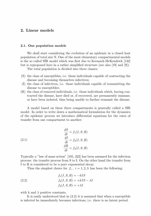
We shall start considering the evolution of an epidemic in a closed hostpopulation of total size N. One of the most elementary compartmental modelsis the so called SIR model which was first due to Kermack-McKendrick [132]but is reproposed here in a rather simplified structure (see also [19] and [9]).

The total population is divided into three classes:

(S) the class of susceptibles, i.e. those individuals capable of contracting thedisease and becoming themselves infectives;

(I) the class of infectives, i.e. those individuals capable of transmitting thedisease to susceptibles;

(R) the class of removed individuals, i.e. those individuals which, having con-tracted the disease, have died or, if recovered, are permanently immune,or have been isolated, thus being unable to further transmit the disease.

A model based on these three compartments is generally called a SIRmodel. In order to write down a mathematical formulation for the dynamicsof the epidemic process we introduce differential equations for the rates oftransfer from one compartment to another:

(2.1)

dS

dt= f1(I, S,R)

dI

dt= f2(I, S,R)

dR

dt= f3(I, S,R)

Typically a ”law of mass action” [105, 222] has been assumed for the infectionprocess: the transfer process from S to I. On the other hand the transfer fromI to R is considered to be a pure exponential decay.

Thus the simplest choice for fi , i = 1, 2, 3 has been the following:

(2.2)

f1(I, S,R) = −kIS

f2(I, S,R) = +kIS − λI

f3(I, S,R) = +λI

with k and λ positive constants.It is easily understood that in (2.2) it is assumed that when a susceptible

is infected he immediately becomes infectious, i.e. there is no latent period.

If latency is allowed, an additional class (E) of latent individuals may beincluded (see Section 3).

2.1.1. SIR model with vital dynamics

In the above formulation the total population

(2.3) N = S + I + R

is a constant, as can be seen by simply adding the three equations in (2.2).The invariance of the total population can be maintained if we introduce

an intrinsic vital dynamics of the individuals in the total population by meansof a net mortality µN compensated by an equal birth input in the susceptibleclass.

In this case (2.2) are substituted by:

(2.4)

f1(I, S,R) = −kIS − µS + µN

f2(I, S,R) = +kIS − λI − µI

f3(I, S,R) = λI − µR

In fact, it is easy to check that

(2.5) N(t) = S(t) + I(t) + R(t)

is again constant in time.We shall assume model (2.4) as a convenient point of departure for subse-

quent analysis, since it already contains the basic features of a general epidemicsystem, including the possibility of a nontrivial steady state as we shall seelater.

System (2.1) together with (2.4) becomes,

(2.6)

dS

dt= −kIS − µS + µN

dI

dt= kIS − µI − λI

dR

dt= λI − µR

for t > 0 , which has to be subject to suitable initial conditions.In this same class other models can be introduced. We shall list the most

well known. From now on, when constant in time, the total population N willbe assumed equal to 1, so that we refer to fractions of the total population.For a discussion about the related values of the parameters, refer to [118].

8 2. Linear models

The SIR model with vital dynamics will then be rewritten as follows:

(2.6′)

dS

dt= −kIS − δS + δ

dI

dt= kIS − γI − δI

dR

dt= γI − δR

We may notice that the first two equations may be solved independently of thethird one. Thus we shall be limiting ourselves to a two-dimensional system.

The same will be done in other cases without further advice.

2.1.2. SIRS model with temporary immunity [110]

This model derives from the SIR model with vital dynamics, but recoverygives only a temporary immunity

(2.7)

dS

dt= −kIS + δ − δS + αR

dI

dt= kIS − (γ + δ)I

dR

dt= γI − αR

2.1.3. SIR model with carriers [110]

A carrier is an individual who carries and spreads the infectious disease,but has no clinical symptoms. If we assume that the number C of the carriersin the population is constant, we modify accordingly the SIR model with vitaldynamics,

(2.8)

dS

dt= −k(I + C)S + δ − δS

dI

dt= k(I + C)S − (γ + δ)I

dR

dt= γI − δR


2.1.4. The general structure of bilinear systems

According to a recent formulation due to Beretta and Capasso [28] all ofthe above models can be written in the general form:

(2.9)dz

dt= diag(z)(e + Az) + c

where

z ∈ IRn, n being the number of different compartments

e ∈ IRn, is a constant vector

A = (aij)i,j=1,...,nis a real constant matrix

c ∈ IRn, is a constant vector.

In the above examples we have in fact:

- SIR model with vital dynamics (model (2.6))

(2.10) A =

(0 −kk 0

); e =

(−δ

−(δ + γ)

); c =

(δ0

)

10 2. Linear models

- SIRS model with temporary immunity (model (2.7))

For our convenience, we change the variables (S, I) into (S, I) such that

S = S +α

k.

Again, by taking into account that S +R+ I = 1 (constant in time), wemay ignore the equation for R.

Thus system (2.1) becomes:

(2.11)

dS

dt= −(δ + α)S − kSI + (δ + α)

(1 +

α

k

)

dI

dt= −(γ + δ + α)I + kSI

so that

A =

(0 −kk 0

); e =

(−(δ + α)

−(γ + δ + α)

); c =

(δ + α)

(1 +

α

k

)

0

- SIR model with carriers (model 2.8)).

We change the variables (S, I) into (S, I), with I = I +C, so that system(2.8) becomes, ignoring the equation for R,

(2.12)

dS

dt= −δS − kIS + δ

dI

dt= −(γ + δ)I + kIS + (γ + δ)C

Hence

A =

(0 −kk 0

); e =

(−δ

−(γ + δ)

); c =

(δ

(γ + δ)C

)

A further extension of the form (2.9) is needed to include the followingmodel.

- SIR model with vertical transmission

A model has been proposed in [40] which extends the SIR model withvital dynamics to include vertical transmission and possible vaccination. Itis assumed that b and b′ are the rates of birth of uninfected and infectedindividuals respectively; r and r′ are the corresponding death rates; v is the


rate of recovery from infection; γ is the rate at which immune individualsloose immunity; q is the rate of vertical transmission (p + q = 1); and m isthe fraction of those born to uninfected parents which are immune because ofvaccination, the rest going into a susceptible class. It has been assumed thatthe vaccine is not effective for the children of infected parents.

The ODE system which describes mathematically such a model is thenthe following,

(2.13)

dS

dt= −kSI + (1 − m)b(S + R) + pb′I − rS + γR

dI

dt= kSI + qb′I − r′I − vI

dR

dt= vI − (r + γ) R + mb(S + R)

In order to keep a constant total population S + I +R = 1 , it is assumed thatb = r, b′ = r′. In this last case the above model reduces to

(2.14)

dS

dt= −kSI + (1 − m)b(1 − I) + pb′I − rS + γR

dI

dt= kSI − (pb′ + v)I

If we set

A =

(0 −kk 0

); e =

(−b − γ−pb′ − v

)

c =

((1 − m)b + γ

0

); B =

(0 (m − 1)b + pb′ + γ0 0

)

system (2.14) can be written in the form

(2.15)dz

dt= diag(z)(e + Az) + c + Bz

which extends equation (2.9) to include the term Bz.This kind of approach of a unifying mathematical structure of epidemic

systems can be further carried out by analyzing epidemic models in two ormore interacting populations.

12 2. Linear models

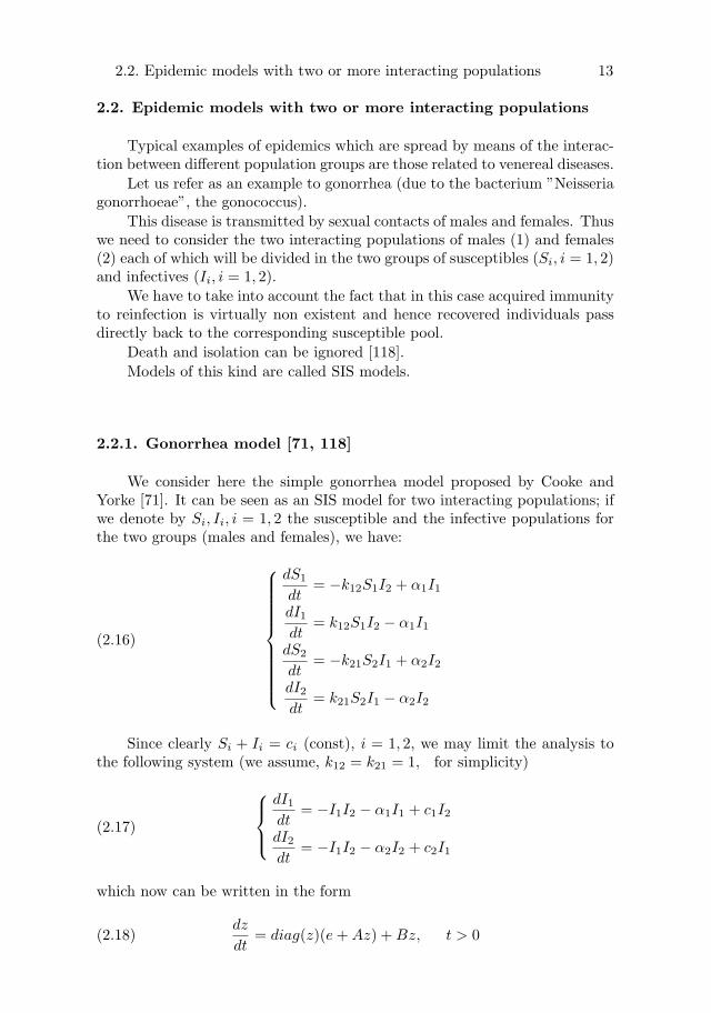
2.2. Epidemic models with two or more interacting populations

Typical examples of epidemics which are spread by means of the interac-tion between different population groups are those related to venereal diseases.

Let us refer as an example to gonorrhea (due to the bacterium ”Neisseriagonorrhoeae”, the gonococcus).

This disease is transmitted by sexual contacts of males and females. Thus

(2) each of which will be divided in the two groups of susceptibles (Si, i = 1, 2)and infectives (Ii, i = 1, 2).

We have to take into account the fact that in this case acquired immunityto reinfection is virtually non existent and hence recovered individuals passdirectly back to the corresponding susceptible pool.

Death and isolation can be ignored [118].

Models of this kind are called SIS models.

2.2.1. Gonorrhea model [71, 118]

We consider here the simple gonorrhea model proposed by Cooke andYorke [71]. It can be seen as an SIS model for two interacting populations; ifwe denote by Si, Ii, i = 1, 2 the susceptible and the infective populations forthe two groups (males and females), we have:

(2.16)

dS1dt

= −k12S1I2 + α1I1

dI1dt

= k12S1I2 − α1I1

dS2dt

= −k21S2I1 + α2I2

dI2dt

= k21S2I1 − α2I2

Since clearly Si + Ii = ci (const), i = 1, 2, we may limit the analysis tothe following system (we assume, k12 = k21 = 1, for simplicity)

(2.17)

dI1dt

= −I1I2 − α1I1 + c1I2

dI2dt

= −I1I2 − α2I2 + c2I1

which now can be written in the form

(2.18)dz

dt= diag(z)(e + Az) + Bz, t > 0

13

we need to consider the two interacting populations of males (1) and females


if we set z = (I1, I2)T

, and

A =

(0 −1−1 0

), e =

(−α1−α2

), B =

(0 c1c2 0

)

2.2.2. SIS model in two communities with migration [110]

In a SIS system with vital dynamics the population is divided into twocommunities; individuals migrate between the two groups. We describe eachcommunity by (Si, Ii) , i = 1, 2 such that

(2.19) Si + Ii = 1 , i = 1, 2 .

Hence we may limit the analysis to the following ODE system:

(2.20)

dI1dt

= k1I1 (1 − I1) − γ1I1 − δ1I1 + θ1 (I2 − I1)

dI2dt

= k2I2 (1 − I2) − γ2I2 − δ2I2 + θ2 (I1 − I2)

Note that the migration terms θi (Ij − Ii) , i, j = 1, 2, i 6= j, are intendedto have an homogeneization effect between the two groups.

Models of this kind are used in ecological systems to describe populationsthat are divided in patches among which discrete diffusion occurs [148, 177,206].

System (2.20) can be written as

(2.21)

dI1dt

= (k1 − γ1 − δ1 − θ1) I1 − k1I12 + θ1I2

dI2dt

= (k2 − γ2 − δ2 − θ2) I2 − k2I22 + θ2I1

which can be put in the form (2.18) if we set

z = (I1, I2)T

,

and

A =

(−k1 00 −k2

), e =

(k1 − γ1 − δ1 − θ1k2 − γ2 − δ2 − θ2

), B =

(0 θ1θ2 0

)

14 2. Linear models

2.2.3. SIS model for two dissimilar groups [110, 142, 218]

In this case the population is divided into two dissimilar groups becauseof age, social structure, space structure, etc.. The two groups may interactwith each other via the infection process; e.g. the force of infection acting onthe susceptibles S1 of the first group will given by

g1 (I1, I2) = k11I1 + k12I2

and the analogous for the other group.

Thus the epidemic system is described by the following set of ODE’s:

(2.22)

dI1dt

= (k11I1 + k12I2) (1 − I1) − γ1I1 − δ1I1

dI2dt

= (k21I1 + k22I2) (1 − I2) − γ2I2 − δ2I2

which can be also written as

(2.23)

dI1dt

= (k11 − γ1 − δ1) I1 − k11I12 − k12I1I2 + k12I2

dI2dt

= (k22 − γ2 − δ2) I2 − k22I22 − k21I2I1 + k21I1

complemented by

I1 + S1 = 1, I2 + S2 = 1

System (2.23) can be put again in the form (2.18) if we define

A =

(−k11 −k12−k21 −k22

); e =

(k11 − γ1 − δ1k22 − γ2 − δ2

); B =

(0 k12

k21 0

).

This case is a particular case (two groups) of the more general case (n groups,n ≥ 2) analyzed by Lajmanovich and Yorke in [142]. We shall deal with thismultigroup case in Section 2.3.4 , or better in Section 4.6.1 .


2.2.4. Host - vector - host model [110]

In an SIS epidemic system with vital dynamics let us suppose that aunique vector is responsible for the spread of the disease among two differenthosts.

In such a case we have three classes of infectives (two hosts and onevector). The force of infection acting on the vector susceptible population(S2) is due to the infectives I1 and I3 of the host.

g2 (I1, I3) = k21I1 + k23I3

while the force of infection acting on the two hosts S1 and S3 due to the vectoris given, respectively, by

g1 (I2) = k12I2

g3 (I2) = k32I2

As a consequence , by assuming, as usual in a SIS model, that

(2.24) Si + Ii = const (= 1), i = 1, 2, 3

we have

(2.25)

dI1dt

= k12I2 (1 − I1) − γ1I1 − δ1I1

dI2dt

= (k21I1 + k23I3) (1 − I2) − γ2I2 − δ2I2

dI3dt

= k32I2 (1 − I3) − γ3I3 − δ3I3

complemented by (2.24).It is more convenient to rewrite system (2.24), (2.25) by emphasizing the

susceptible populations Si = 1 − Ii, which gives

(2.26)

dS1dt

= (−k12 − (γ1 + δ1)) S1 + k12S1S2 + (γ1 + δ1)

dS2dt

= (−k21 − k23 − (γ2 + δ2)) S2 + k21S2S1 + k23S2S3

+ (γ2 + δ2)

dS3dt

= (−k32 − (γ3 + δ3)) S3 + k32S3S2 + (γ3 + δ3) .

System (2.26) can be put in the form (2.9) if we set

A =

0 k12 0

k21 0 k230 k32 0

;

e =

−k12 − (γ1 + δ1)

−k21 − k23 − (γ2 + δ2)−k32 − (γ3 + δ3)

; c =

γ1 + δ1

γ2 + δ2γ3 + δ3

.

16 2. Linear models

2.3. The general structure

To include the models listed in Sections 2.1 and 2.2 we need to generalize(2.9) and write it in the more general form

(2.27)dz

dt= diag(z)(e + Az) + b(z)

where now

(2.28) b(z) = c + Bz

with

(i) c ∈ IRn+

a constant vector

and

(ii) B = (bij)i,j=1,...,na real constant matrix such that

bij ≥ 0, i, j = 1, . . . , n

bii = 0, i = 1, . . . , n

For system (2.27) we shall give a detailed analysis of the asymptotic behaviorbased on recent results due to Beretta and Capasso [28].


2.3.1. Constant total population

We consider at first the case in which the total population N is constant.A direct consequence is that any trajectory

z(t), t ∈ IR+

of system

(2.27) is contained in a bounded domain Ω ⊂ IRn :

(A1) Ω is positively invariant.

Because of the structure of F : IRn → IRn defined by

(2.29) F (z) := diag(z)(e + Az) + b(z)

it is clear that F ∈ C1 (Ω) .We shall denote by Di the hyperplane of IRn :

Di = z ∈ IRn | zi = 0 , i = 1, . . . , n .

Clearly, for any i = 1, . . . , n , Di ∩ Ω will be positively invariant if bi |Di=

0, while Di ∩ Ω will be a repulsive set whenever bi |Di> 0, in which case

F (z) will be pointing inside Ω on Di.Because of the invariance of Ω and the fact that F ∈ C1 (Ω), standard

fixed point theorems [180] (Appendix B, Section B.1) assure the existence ofat least one equilibrium solution of (2.27), within Ω.

Suppose now that a strictly positive equilibrium z∗ exists for system(2.27) (z∗i > 0, i = 1, . . . , n):

diag (z∗) (e + Az∗) + b (z∗) = 0

from which we get

(2.30) e = −Az∗ − diag(z∗−1

)b (z∗)

where we have denoted by

z∗−1 :=

(1

z∗1

, . . . ,1

z∗n

)T

By substitution into (2.27), we get

(2.31)

dz

dt= diag(z)

[A + diag

(z∗−1

)B](z − z∗)

− diag (z − z∗) diag(z∗−1

)b(z)

18 2. Linear models

Since (2.27) is a Volterra like system we may make use of the classicalVolterra-Goh Lyapunov function [96].

(2.32) V (z) :=

n∑i=1

wi

(zi − z∗i − z∗i ln

zi

z∗i

), z ∈ IRn∗

where wi > 0, i = 1, . . . , n , are real constants (the weights).Here we denote by

IRn∗+

:= z ∈ IRn | zi > 0, i = 1, . . . , n ,

and clearlyV : IRn∗

+→ IR+ .

The derivative of V along the trajectories of (2.27) is given by

(2.33) V (z) = (z − z∗)T

WA (z − z∗) −n∑

i=1

wi

bi(z)

ziz∗i(zi − z∗i )

2, z ∈ IRn∗

+

which can be rewritten as

(2.34) V (z) = (z − z∗)T

W

[A + diag

(−b1(z)

z1z∗1, . . . ,

−bn(z)

znz∗n

)](z − z∗)

We have denoted by W := diag(w1, . . . , wn), and by

(2.35) A := A + diag(z∗−1

)B .

The structure of (2.33) and (2.34) stimulates the analysis of the following twocases:

(A) A is W-skew symmetrizable

(B) −

[A + diag

(−b1(z)

z1z∗1, . . . ,

−bn(z)

znz∗n

)]∈ SW .

We say that a real n × n matrix A is ”skew-symmetric” if AT = −A.We say that a real n × n matrix A is W -skew symmetrizable if there

exists a positive diagonal real matrix W such that WA is skew-symmetric.We say that a real n×n matrix A is in SW (resp. ”Volterra-Lyapunov

stable”) if there exists a positive diagonal real matrix W such that WA +AT W is positive definite (resp. negative definite).

In case (B)V (z) ≤ 0, z ∈ IRn∗

+

and the equality applies if and only if z = z∗. The global asymptotic stabilityof z∗ follows from the classical Lyapunov theorem (Appendix A, Section A.5).Thus we have proved the following

Theorem 2.1. If system (2.27) admits a strictly positive equilibrium z∗ ∈Ω(zi > 0, i = 1, . . . , n) and condition (B) applies, then z∗ is globally asymp-totically stable within Ω. The uniqueness of such an equilibrium point followsfrom the GAS.


Consider case (A) now. Since WA is skew-symmetric, from (2.33) we get

(2.36) V (z) = −n∑

i=1

wibi(z)


2

Since bi(z) ≥ 0 for any z ∈ IRn∗+

, i = 1, . . . , n , we have

V (z) ≤ 0 .

Denote by R ⊂ Ω the set of points where V (z) = 0; clearly

(2.37) R = z ∈ Ω | zi = z∗i if bi(z) > 0, i = 1, . . . , n

We shall further denote by M the largest invariant subset of R. By the LaSalleInvariance Principle [145] (Appendix A, Section A.5) we may then state thatevery solution tends to M for t tending to infinity.

In order to give more information about the structure of M , we refer tograph theoretical arguments [205].

Since in case (A) the elements of A have a skew-symmetric sign distribu-tion, we can then associate a graph with A by the following rules.

(α) each compartment i ∈ 1, . . . , n is represented by a labelled knot denotedby

(a.1) ”” if bi(z) = 0 ∀z ∈ Ω

(a.2) ”•” otherwise

(β) if a pair of knots (i, j) is such that ai,j aj,i < 0 then the two knots i andj are connected by an arc (see for examples Sect. 2.3.1.1).

The following lemma holds [205].

Lemma 2.2. Assume that A is skew-symmetrizable. If the associated graphis either

(a) a tree and ρ − 1 of the terminal knots are •or

(b) a chain and two consecutive internal knots are •or

(c) a cycle and two consecutive knots are •

then M = z∗ within R.

As a consequence of this lemma and the above arguments we may statethe following

Theorem 2.3. If system (2.27) admits a strictly positive equilibrium z∗ ∈Ω (z∗i > 0, i = 1, . . . , n) and condition (A) applies under one of the as-sumptions of Lemma 2.2, then the positive equilibrium z∗ is GAS within Ω(again the uniqueness of z∗ follows from its GAS).

20 2. Linear models

The interest of Theorems 2.1. and 2.3. lies in the fact that they providesufficient conditions in order that an equilibrium solution of system (2.27) beglobally asymptotically stable whenever we are able to show that it exists.

This will reduce a problem of GAS to an ”algebraic” problem. On theother hand necessary and sufficient conditions for the existence of an equi-librium solution usually include ”threshold” conditions on the parameters forthe existence of such a nontrivial endemic state.

Sufficient conditions for the existence of a nontrivial endemic state aregiven in the following corollary of Theorems 2.1. and 2.3.

Corollary 2.4. If the vector c in (2.28) (i) is strictly positive, then the system(2.27) admits a strictly positive equilibrium z∗ ∈ Ω+. In either cases (A) and(B), the positive equilibrium z∗ is GAS (and therefore unique) with respectto Ω+.

An extension of these results to the space heterogeneous case can be foundin Sect. 5.6.

2.3.1.1. Case A: epidemic systems for which the matrix A is W-skew

symmetrizable

2.3.1.1.1. SIR model with vital dynamics

It is clearly seen from (2.35) that, since in this case B = 0, we have A = A

and b(z) = c =

(δ0

).

A is thus skew-symmetric and the associated graph is •––. Theorem 2.3.applies.

In this case the nontrivial equilibrium point, i.e. the nontrivial endemicstate, is given by

(2.38) S∗ =γ + δ

k; I∗ =

δ

k

(1

S∗− 1

)

which exists iff

(2.39) σ =k

γ + δ> 1.

Note that if σ ≤ 1 then the only equilibrium point of the system is (1, 0)T,

and this is GAS.


2.3.1.1.2. SIRS model with temporary immunity

Again in this case

A = A and b(z) = c

so that A is skew-symmetric. The associated graph is also •––, and Theorem2.3. applies.

In this case the nontrivial endemic state is given by z∗ = (S∗, I∗)T, where

S∗ =γ + δ

k=:

1

σ

I∗ =(δ + α) (σ − 1)

k + ασ

which exists iff σ > 1.Otherwise, for σ ≤ 1, the only equilibrium point of the system is (1, 0)

T.

2.3.1.1.3. SIR model with carriers

In this caseA = A and b(z) = c.

Since c is positive definite and A is skew-symmetric, we may apply Corollary2.4 to state that a unique positive equilibrium z∗ exists,which is GAS withrespect to the interior of

Ω :=

z =

(S, I)T

∈ IR2+| S + I ≤ 1 + C

In this case then an endemic state always exists. Its coordinates are given by[110]

S∗ = 1 −kI∗

δσ

I∗ =δ

2k

(

σ − 1 − Ck

δ

)+

((σ − 1 − C

k

δ

)2+ 4C

kσ

δ

) 1

2

where, as usual, σ :=k

γ + δ.

22 2. Linear models

2.3.1.1.4. SIR model with vertical transmission

In this case b(z) = c + Bz.

Moreover this system admits the following equilibrium point

(2.40)

S∗ =pb′ + v

k

I∗ =((1 − m)b + γ) k − (b + γ) (pb′ + v)

(v + (1 − m) b + γ) k

This is a nontrivial endemic state (I∗ > 0) iff

(2.41) m <(b + γ) (k − pb′ − v)

bk.

As a consequence

A := A + diag(z∗−1

)B =

0 k

(m − 1)b − γ − v

p b′ + v

k 0

Now, (m − 1)b, −γ, −v are all nonpositive quantities. We assume, toexclude extreme cases, that they are all negative. Thus a suitable positivediagonal matrix W = diag(w1w2) can be easily shown to exist, such that

WA reduces to

(0 −kk 0

). We fall into case (A) Section 2.3.1. Since the

associated graph is •––, the endemic state (2.40) (under (2.41)) is GAS.


2.3.1.2.1. Gonorrhea model

In this case (Eqn. (2.17)),

b(z) = Bz =

(c1I2c2I1

), A =

0c1 − I∗

1

I∗1

c2 − I∗2

I∗2

0

consider the matrix

(2.42) W

A + diag

−c1I2

I∗1I1 −

c2I1I∗2I2

=

−w1c1I2I∗1I1

w1S∗

1

I∗1

w2S∗

2

I∗2

−w2c2I1I∗2I2

which is a symmetric matrix if we choose w1 > 0, and w2 > 0 such that

w2

(S∗

2

I∗2

)= w1

(S∗

1

I∗1

)

The symmetric matrix (2.42) is negative definite. In fact the diagonalelements are negative and

(c1I2I∗1I1

c2I1I∗1I2

−S∗

1S∗

2

I∗1I∗2

)w1w2 =

w1w2I∗1I∗2

(c1c2 − S∗

1S∗

2) > 0 ,

where the fact that 0 < S∗

i < ci, i = 1, 2, is taken into account since

z∗ = (I∗1, I∗2)T

is a positive equilibrium. Theorem 2.3 applies.

24 2. Linear models

2.3.1.2. Case B: epidemic systems for which

−

[A + diag

(−

b1(z)

z1z∗1, . . . ,

bn(z)

znz∗n

)]∈ SW .

2.3.1.2.2. SIS model in two communities with migration

This model has been reduced to system (2.21). Hence

b(z) = Bz =

(θ1I2θ2I1

), and A =

−k1θ1I∗1

θ2I∗2

−k2

Let Ω ⊂ IR2 be defined as

Ω :=

z = (I1, I2)T ∈ IR2 | 0 ≤ Ii ≤ 1, i = 1, 2

Because of Theorem 2.3, the sufficient condition for the asymptotic stabilityof a positive equilibrium z∗, with respect to Ω is

−

[A + diag

(−

θ1I2I∗1I1

,−θ2I1I∗2I2

)]∈ SW

We can observe that

(2.43) WA + diag

(−w1

θ1I2I∗1I1

,−w2θ2I1I∗2I2

)

=

−w1θ1I2I∗1I1

w1θ1I∗1

w2θ2I∗2

−w2θ2I1I∗2I2

+ diag (−k1w1,−k2w2)

The first matrix on the right hand side of (2.43) is symmetric if we choose

w1 > 0, w2 =θ1I

∗

2

θ2I∗1w1.

This matrix is negative semidefinite since

(θ1I2I∗1I1

θ2I1I∗2I2

−θ1I∗1

θ2I∗2

)w1w2 = 0 .

Because of the presence of the diagonal negative matrix on the right hand sideof (2.43), the sufficient condition of Theorem 2.3.k1, k2 > 0.

z∗

GAS within Ω.


Under these assumptions, if a positive equilibrium

holds true provided that

exists, then it is

2.3.1.2.3. SIS model for two dissimilar groups

This model has been reduced to the form (2.23).

Hence

b(z) ≡ Bz =

(k12I2k21I1

), A =

−k11k12I∗1

(1 − I∗1)

k21I∗2

(1 − I∗2) −k22

Consider now

(2.44) W

[A + diag

(−

k12I2I∗1I1

,−k21I1I∗2I2

)]

=

−w1k12I2I∗1I1

w1k12I∗1

(1 − I∗1)

w2k21I∗2

(1 − I∗2) −w2

k21I1I∗2I2

+ diag (−k11w1,−k22w2)

where the first matrix on the right hand side of (2.44) is symmetric when

choosing w1 > 0 and w2 such that

(k21I∗2

)(1 − I∗

2) w2 =

(k12I∗1

)(1 − I∗

1) w1.

Moreover, since 0 < I∗i < 1, i = 1, 2, this matrix is negative definite. Infact, (

k12I2I∗1I1

k21I1I∗2I2

−k12I∗1

(1 − I∗1)

k21I∗2

(1 − I∗2)

)w1w2 > 0.

Hence, provided that k11 ≥ 0, k22 ≥ 0,

−

[A + diag

(−

k12I2I∗1I1

,−k21I1I∗2I2

)]∈ SW

and Theorem 2.3. assures the asymptotic stability of the positive equilibriumz∗ with respect to Ω =

z ∈ IR2

+| Ii ≤ 1, i = 1, 2

.

26 2. Linear models

2.3.1.2.4. Host - vector- host model

This model has been reduced to the form (2.26).Hence

b(z) ≡ c , A ≡ A

By Corollary 2.4, since c is a positive definite vector, one positive equilibrium

z∗ exists in

Ω, where

Ω :=z ∈ IR3

+| 0 ≤ Si ≤ 1, i = 1, 2, 3

.

A has a symmetric sign structure. Hence, by Corollary 2.4, if

−

[A + diag

(−(γ1 + δ1)

S1S∗

1

,−(γ2 + δ2)

S2S∗

2

,−(γ3 + δ3)

S3S∗

3

)]∈ SW

then z∗ is asymptotically stable within

Ω. If we take into account that Si ≤1, i = 1, 2, 3, from (2.34) we see that a sufficient condition for the asymptoticstability of z∗ is

−[A + diag (− (γ1 + δ1) ,− (γ2 + δ2) ,− (γ3 + δ3))] ∈ SW .

Accordingly, let us take

W [A + diag (− (γ1 + δ1) ,− (γ2 + δ2) ,− (γ3 + δ3))]

=

− (γ1 + δ1) w1 k12w1 0

k21w2 − (γ2 + δ2) w2 k23w20 k32w3 − (γ3 + δ3) w3

This matrix is symmetric if we choose

w1 > 0, w2 =

(k12k21

)w1, w3 =

(k23k32

)(k12k21

)w1.

It is negative definite if

[(γ1 + δ1) (γ2 + δ2) − k12k21]w1w2 > 0,

(2.45) −[ (γ1 + δ1) (γ2 + δ2) (γ3 + δ3) − (γ3 + δ3) k12k21

− (γ1 + δ1) k23k32]w1w2w3 < 0

We can observe that, if inequalities in (2.45) hold true, then

[(γ2 + δ2) (γ3 + δ3) − k23k32]w2w3 > 0 .


Hence (2.45) is the sufficient condition for the asymptotic stability (and

uniqueness) of the positive equilibrium z∗ within

Ω.From (2.26) the positive equilibrium z∗ has the following components:

(2.46) S∗

1=

γ1 + δ1k12 (1 − S∗

2) + (γ1 + δ1)

, S∗

3=

γ3 + δ3k32 (1 − S∗

2) + (γ3 + δ3)

,

and S∗

2is a solution of

(2.47) (1 − S2)

p(1 − S2)2

+ q (1 − S2) + r

= 0 ,

where

p = k12k32 [(k21 + k23) + (γ2 + δ2)] ,

q = k32 [(γ1 + δ1) (γ2 + δ2) − k12k21] + k12 [(γ2 + δ2) (γ3 + δ3) − k23k32]

+ k12k21 (γ3 + δ3) + k23k32 (γ1 + δ1)

r = (γ1 + δ1) (γ2 + δ2) (γ3 + δ3) − (γ3 + δ3) k12k21 − (γ1 + δ1) k23k32 .

It is to be noticed that when (2.45) holds true, then q > 0, r > 0, thusassuring that the unique asymptotically stable equilibrium is such that S∗

2=

1, i.e. z∗ = (1, 1, 1)T .When (2.45) fails to hold, by (2.47) we have another positive equilibrium

for which S∗

2< 1 and its remaining components are given by (2.46).

To study the asymptotic stability of this equilibrium we can remem-ber that Ii + Si = 1, i = 1, 2, 3, thus assuring to have a positive equi-librium z∗ = (I∗

1, I∗2, I∗3)T

, 0 < I∗i < 1, i = 1, 2, 3 within the subsetΩ =

z ∈ IR3

+: Ii ≤ 0, i = 1, 2, 3

. In the old variables Ii, i = 1, 2, 3, the

positive equilibrium becomes the origin and the ODE system (2.25) can bearranged in this form:

dI1dt

= − (γ1 + δ1) I1 − k12I1I2 + k12I2 ,

dI2dt

= − (γ2 + δ2) I2 − k21I2I1 − k23I2I3 + (k21I1 + k23I3) ,

dI3dt

= − (γ3 + δ3) I3 − k32I3I2 + k32I2

so that

e =

− (γ1 + δ1)

− (γ2 + δ2)− (γ3 + δ3)

, A =

0 −k12 0

−k21 0 −k230 −k32 0

c = 0, B =

0 k12 0

k21 0 k230 k32 0

28 2. Linear models

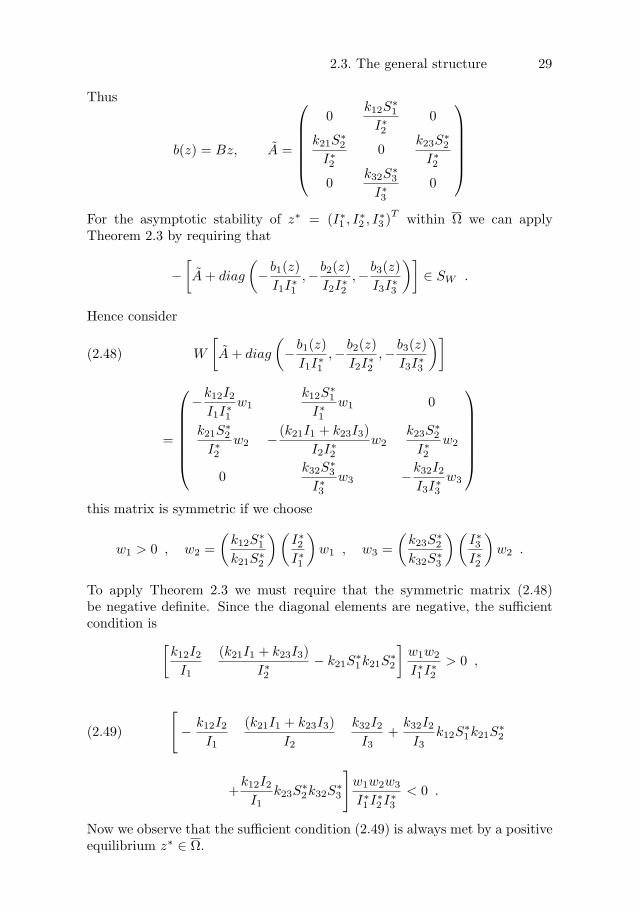
Thus

b(z) = Bz, A =

0k12S

∗

1

I∗2

0

k21S∗

2

I∗2

0k23S

∗

2

I∗2

0k32S

∗

3

I∗3

0

For the asymptotic stability of z∗ = (I∗1, I∗2, I∗3)T

within Ω we can applyTheorem 2.3 by requiring that

−

[A + diag

(−

b1(z)

I1I∗1,−

b2(z)

I2I∗2,−

b3(z)

I3I∗3

)]∈ SW .

Hence consider

(2.48) W

[A + diag

(−

b1(z)

I1I∗1,−

b2(z)

I2I∗2,−

b3(z)

I3I∗3

)]

=

−k12I2I1I∗1

w1k12S

∗

1

I∗1

w1 0

k21S∗

2

I∗2

w2 −(k21I1 + k23I3)

I2I∗2w2

k23S∗

2

I∗2

w2

0k32S

∗

3

I∗3

w3 −k32I2I3I∗3

w3

this matrix is symmetric if we choose

w1 > 0 , w2 =

(k12S

∗

1

k21S∗

2

)(I∗2

I∗1

)w1 , w3 =

(k23S

∗

2

k32S∗

3

)(I∗3

I∗2

)w2 .

To apply Theorem 2.3 we must require that the symmetric matrix (2.48)be negative definite. Since the diagonal elements are negative, the sufficientcondition is

[k12I2

I1

(k21I1 + k23I3)

I∗2

− k21S∗

1k21S

∗

2

]w1w2I∗1I∗2

> 0 ,

(2.49)

[−

k12I2I1

(k21I1 + k23I3)

I2

k32I2I3

+k32I2

I3k12S

∗

1k21S

∗

2

+k12I2

I1k23S

∗

2k32S

∗

3

]w1w2w3I∗1I∗2I∗3

< 0 .

Now we observe that the sufficient condition (2.49) is always met by a positiveequilibrium z∗ ∈ Ω.


In fact

k12I2I1

(k21I1 + k23I3)

I2− k12S

∗

1k21S

∗

2>

k12I2I1

k21I1I2

− k12k21 = 0

and

−k12I2

I1

k21I1I2

k32I2I3

+k32I2

I3k12S

∗

1k21S

∗

2−

k12I2I1

k23I3I2

k32I2I3

+k12I2

I1k23S

∗

2k32S

∗

3=

=I2I3

k32 (−k12k21 + k12S∗

1k21S

∗

2) +

k12I2I1

(−k23k32 + k23S∗

2k32S

∗

3) < 0 ,

where, when proving the inequalities, we have taken into account that S∗

i <1, i = 1, 2, 3.

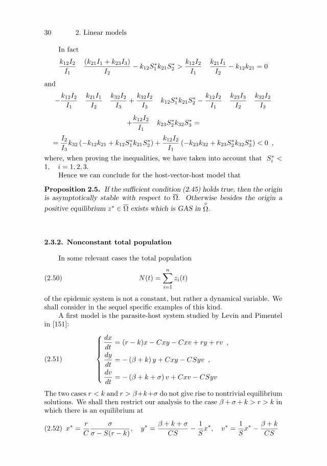
Hence we can conclude for the host-vector-host model that

Proposition 2.5. If the sufficient condition (2.45) holds true, then the originis asymptotically stable with respect to Ω. Otherwise besides the origin a

positive equilibrium z∗ ∈ Ω exists which is GAS in

Ω.

2.3.2. Nonconstant total population

In some relevant cases the total population

(2.50) N(t) =n∑

i=1

zi(t)

of the epidemic system is not a constant, but rather a dynamical variable. Weshall consider in the sequel specific examples of this kind.

A first model is the parasite-host system studied by Levin and Pimentelin [151]:

(2.51)

dx

dt= (r − k)x − Cxy − Cxv + ry + rv ,

dy

dt= − (β + k) y + Cxy − CSyv ,

dv

dt= − (β + k + σ) v + Cxv − CSyv

The two cases r < k and r > β+k+σ do not give rise to nontrivial equilibriumsolutions. We shall then restrict our analysis to the case β + σ + k > r > k inwhich there is an equilibrium at

(2.52) x∗ =r

C

σ

σ − S(r − k), y∗ =

β + k + σ

CS−

1

Sx∗, v∗ =

1

Sx∗ −

β + k

CS

30 2. Linear models

The equilibrium z∗ = (x∗, y∗, v∗) is feasible, i.e. its components are positiveif

(2.53)r

β + k + σ< 1 −

S(r − k)

σ<

r

β + k,

If σ < σ1 where σ1 is such that

(2.54)r

β + k + σ1= 1 −

S(r − k)

σ1,

the first inequality in (2.53) is violated and only a partially feasible equilibriumis present given by

(2.55) x∗ =β + k + σ

C, y∗ = 0, v∗ =

r − k

β + k + σ + rx∗

since r < β + k + σ. If σ = σ1 then (2.52) coalesces in (2.55). If r < β + kand σ > σ2 , where σ2 is such that

(2.56) 1 −S(r − k)

σ2=

r

β + k

then the second inequality in (2.53) is violated and only a partially feasibleequilibrium is present, given by

(2.57) x∗ =β + k

C, y∗ =

r − k

β + k − rx∗, v∗ = 0

since r > k. If σ = σ2 then (2.52) coalesces in (2.57).Concerning system (2.51), if we denote by z = (x, y, v)T and set

A =

0 −C −C

C 0 −CSC CS 0

; e =

r − k

− (β + k)− (β + k + σ)

c = 0, B =

0 r r

0 0 00 0 0

we may reduce it again to the general structure (2.27), but in this case

(2.58)dN

dt= (r − k)N(t)

and the evolution of system (2.51) has to be analyzed in the whole IR3+.

Local stability results were already given in [151]. Here we shall studyglobal asymptotic stability of the feasible or partially feasible equilibrium bythe Beretta-Capasso approach (see Section 2.3.2.1).


A second model that we shall analyze is the SIS model with vital dynam-ics, which is proposed by Anderson and May [8]

(2.59)

dS

dt= (r − b)S − ρSI + (µ + r) I

dI

dt= − (θ + b + µ) I + ρSI

If we denote by z = (S, I)T and set

A =

(0 −ρρ 0

); e =

(r − b

− (θ + b + µ)

)

c = 0; B =

(0 µ + r0 0

)

we go back to system (2.27). In this case

dN

dt(t) = (r − b)N(t) − θI(t)

Other examples will be discussed later. It is clear that if the total populationis a dynamical variable rather than a specified constant, we need to dropassumption (A1) in Section 2.3.1.

For these systems the accessible space is the whole nonnegative orthantIRn+

of the Euclidean space. We cannot apply then the standard fixed pointtheorems.

We can only assume that

(A2) IRn+

is positively invariant.

We shall give now more extensive treatment of system (2.27) includingthe possibility of partially feasible equilibrium points.

We shall say that z∗ is a partially feasible equilibrium whenever anonempty proper subset of its components are zero. If we denote by N =1, . . . , n, we mean that a set I ⊂ N exists, such that I 6= ∅, I 6= N andz∗i = 0 for any i ∈ I.

Assume from now on that this is the case; given the matrices

A = (aij)i,j=1,...,nand B = (bij)i,j=1,...,n

in system (2.27), we define a new matrix

A = (aij)i,j=1,...,n

32 2. Linear models

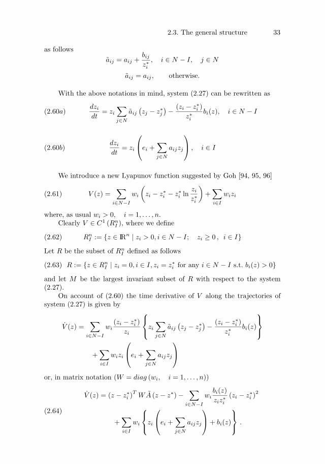
as follows

aij = aij +bij

z∗i, i ∈ N − I, j ∈ N

aij = aij , otherwise.

With the above notations in mind, system (2.27) can be rewritten as

(2.60a)dzi

dt= zi

∑j∈N

aij

(zj − z∗j

)−

(zi − z∗i )

z∗ibi(z), i ∈ N − I

(2.60b)dzi

dt= zi

ei +

∑j∈N

aijzj

, i ∈ I

We introduce a new Lyapunov function suggested by Goh [94, 95, 96]

(2.61) V (z) =∑

i∈N−I

wi

(zi − z∗i − z∗i ln

zi

z∗i

)+∑i∈I

wizi

where, as usual wi > 0, i = 1, . . . , n.Clearly V ∈ C1 (Rn

I ), where we define

(2.62) RnI := z ∈ IRn | zi > 0, i ∈ N − I; zi ≥ 0 , i ∈ I

Let R be the subset of RnI defined as follows

(2.63) R := z ∈ RnI | zi = 0, i ∈ I, zi = z∗i for any i ∈ N − I s.t. bi(z) > 0

and let M be the largest invariant subset of R with respect to the system(2.27).

On account of (2.60) the time derivative of V along the trajectories ofsystem (2.27) is given by

V (z) =∑

i∈N−I

wi

(zi − z∗i )

zi

zi

∑j∈N

aij

(zj − z∗j

)−

(zi − z∗i )

z∗ibi(z)

+∑i∈I

wizi

ei +

∑j∈N

aijzj

or, in matrix notation (W = diag (wi, i = 1, . . . , n))

(2.64)

V (z) = (z − z∗i )T

WA (z − z∗) −∑

i∈N−I

wi

bi(z)


2

+∑i∈I

wi

zi

ei +

∑j∈N

aijzj

+ bi(z)

.


It is clear that

R =

z ∈ RnI | V (z) = 0

.

We are now in a position to state the following

Theorem 2.6. Let z∗ be a partially feasible equilibrium of system (2.27),with z∗i = 0 for i ∈ I ⊂ N, I 6= ∅, I 6= N . Assume that

(a) A is W-skew symmetrizable

(b) ei +∑

j∈N aijz∗

j ≤ 0, i ∈ I

(c) bi(z) ≡ 0, i ∈ I

(d) M ≡ z∗

Then z∗ is globally asymptotically stable within RnI .

Proof. Since A is W-skew symmetrizable, the first term in (2.64) vanishes. Bythe assumptions (b), V (z) ≤ 0 in Rn

I . We can then apply LaSalle InvariancePrinciple [145, Theorem VI Sect. 13 (see also Appendix A, Section A.5)],tostate that z∗ is GAS in Rn

I .

A natural consequence of Theorem 2.6 is the following

Corollary 2.7. Let z∗ be a feasible equilibrium of (2.27) and assume thatA is W-skew symmetrizable. If M ≡ z∗ then z∗ is globally asymptoticallystable within IRn∗

+.

Corollary 2.7 can be seen as a new formulation of Theorem 2.3 in the casein which (A1) is substituted by (A2).

Under the same conditions of this corollary we can also observe that ifthe graph associated with A by means of (α) and (β) satisfies anyone of thehypotheses in Lemma 2.2, then within R we have M ≡ z∗.

We can now solve the two models presented in Section 2.3.1.

34 2. Linear models

2.3.2.1. The parasite-host system [151]

Consider the case in which the equilibrium (2.52) is feasible, i.e. z∗ ∈ IR3+

.Then

(2.65) b(z) ≡ Bz, A =

0 −(C −

r

x∗

)−(C −

r

x∗

)

C 0 −CS

0 CS 0

where z is a vector z = (x, y, v)T

belonging to the non-negative orthant

IR3+

. Since C −r

x∗= CS

(r − k)

σprovided that r > k, matrix A is W-skew

symmetrizable by the diagonal positive matrix W = diag (w1, w2, w3), where

w1 =σ

S(r − k), w2 = w3 = 1. In fact, we obtain

WA =

0 −C −C

C 0 −CSC CS 0

Now we are in position to apply Corollary 2.7.Since b(z) = (r(y + z), 0, 0)T , the subset of all points within IRn∗

+where

we have V (z) = 0 , is

R =z ∈ IRn

+| x = x∗

Now we look for the largest invariant subset M within R . Since x = x∗

for all t ,dx

dt

∣∣∣∣R

= 0 , and from the first of the Eqns. (2.51) we obtain

(y + v) |R=r − k

C −r

x∗

=σ

CS, for all t.

Therefore,d(y + v)

dr

∣∣∣∣R

= 0, and by the last two Eqns. (2.51) we obtain

z |R=1

σ[Cx∗ − (β + k)] [(y + v)]R =

1

CS[Cx∗ − (β + k)] =

x∗

S−

β + k

CS

Then, by taking into account (2.52) we have z |R≡ z∗.


Immediately follows

y |R=σ

CS− v∗ =

β + k + σ

CS−

x∗

S,

i.e. y |R= y∗. Then the largest invariant set M within R is z∗. From Corollary2.7 it follows the global asymptotic stability of the feasible equilibrium (2.52)within IR3∗

+.

It is to be noticed that the only assumptions made in this proof are r > kand that equilibrium (2.52) is feasible. Under these assumptions we excludethat unbounded solutions may exist.

Suppose that σ ≤ σ1, i.e. the equilibrium (2.52) is not feasible and weget the partially feasible equilibrium (2.55) which belongs to

R32

=z ∈ IR3 | zi > 0, i = 1, 3, z2 ≥ 0

In order to apply Theorem 2.6, hypotheses (a) and (b) must be verified.Concerning hypothesis (a), we have

(2.66) − (β + k) + cx∗ − cSv∗ ≤ 0 ,

from which, by taking into account (2.55), we obtain

(2.67) 1 −S(r − k)

σ≤

r

β + k + σ,

Inequality (2.67) is satisfied in the whole range σ ≤ σ1 within which thepartially feasible equilibrium (2.55) occurs. When σ = σ1 the equality appliesin (2.53). Hypothesis (b) is satisfied because b(z) = (r(y + v), 0, 0)T andtherefore b2(z) ≡ 0. Concerning hypothesis (c), consider first the case σ < σ1,i.e. the inequality applies in (2.53).

Then the subset (2.63) is

R =z ∈ R3

2| y = 0, x = x∗

.

Now we look for the largest invariant subset M within R.

Since x = x∗, y = 0 for all t ,dx

dt

∣∣∣∣R

= 0, and from the first of equation

(2.51) we get

36 2. Linear models

v |R=r − k

C −r

x∗

where x∗ =β + k + σ

C.

Therefore, we obtain v |R=

[(r − k)

(β + k + σ − r)

]x∗, i.e. v |R≡ v∗. Thus

the largest invariant set within R is

z∗ =

(x∗ =

β + k + σ

C, y∗ = 0, v∗ =

r − k

β + k + σ − rx∗

)T

.

When σ = σ1, then equality applies in (2.53), and (2.63) becomes

R =z ∈ R3

2| x = x∗

.

In this case, we have already proven that M ≡ z∗. Hence hypothesis(c) is satisfied. Then by Theorem 2.6 the partially feasible equilibrium (2.55)is globally asymptotically stable with respect to R3

2.

If r < β + k and σ ≥ σ2, then the partially feasible equilibrium (2.57)occurs. This equilibrium belongs to

R33

=z ∈ IR3

+| zi > 0, i = 1, 2; z3 ≥ 0

.

Hypothesis (a) of Theorem 2.6 requires

(2.68) − (β + k + σ) + Cx∗ + CSy∗ ≤ 0 ,

from which, by taking into account (2.57), we obtain

(2.69) 1 −S(r − k)

σ≥

r

β + k.

This inequality is satisfied in the whole range of existence of the equilib-rium (2.57), i.e. for all σ ≥ σ2.

When σ = σ2, the equality applies in (2.69). Hypothesis (b) of Theorem2.6 is obviously satisfied. Concerning hypothesis (c), at first we consider thecase in which σ > σ2. Therefore, the inequality applies in (2.68) and thesubset (2.63) of R3

3is


R =z ∈ R3

3| v = 0, x = x∗

.

From (2.57), we are ready to prove that M ≡ z∗. When σ = σ2, Rbecomes

R =z ∈ R3

3| z = x∗

,

and we have already proven that M ≡ z∗. Hypothesis (c) is satisfied. Also,in this case Theorem 2.6 assures the global asymptotic stability of the partiallyfeasible equilibrium (2.57) with respect to R3

3.

Extensions of this model, which have raised further open mathematicalproblems, are due to Levin [149, 150].

2.3.2.2. An SIS model with vital dynamics

Provided that r > b, θ > r−b, system (2.59) has the feasible equilibriumz∗ ∈ IR2∗

+:

(2.70) S∗ =θ + b + µ

ρ, I∗ =

r − b

θ + b − rS∗.

When r ≤ b, or r > θ + b, the equilibrium (2.70) is not feasible and theonly equilibrium of (2.59) is the origin.

Here b(z) ≡ Bz = ((µ + r) I, 0)T. When z∗ is a feasible equilibrium the

matrix A = A + diag(z∗−1

)B is given by

A =

(0 −

(ρ −

µ + r

S∗

)

ρ 0

)

Since S∗ =(θ + b + µ)

ρ, provided that θ > r − b the matrix A is skew-

symmetrizable. Because b1(z) ≥ 0, the graph associated with A is •––, and byCorollary 2.7 the global asymptotic stability of z∗ with respect to IR2

+follows.

When r ≤ b, r > θ + b Theorem 2.6 cannot be applied to studyattractivity of the origin because hypothesis (b) is violated.

38 2. Linear models

2.3.2.3. An SIRS model with vital dynamics in a population with

varying size [44]

As a generalization of the model discussed in Sect. 2.1.2 and Sect.2.3.1.1.2, in [44] Busenberg and van den Driessche propose the following SIRSmodel

(2.71)

dS

dt= bN − dS −

λ

NIS + eR

dI

dt= −(d + ǫ + c)I +

λ

NIS

dR

dt= −(d + δ + f)R + cI

for t > 0 , subject to suitable initial conditions.In this case the evolution equation for the total population N is the fol-

lowing one,

(2.72)dN

dt= (b − d)N − ǫI − δR , t > 0 .

We may notice that whenever b 6= d, N is a dynamical variable. It is thenrelevant to take it into explicit account in the force of infection.

If we take into account the discussion in [110] and [118], we may realizethat also model (8)-(10) in [6] should be rewritten as (2.71).

The biological meaning of the parameters in (2.71) is the following :

b = per capita birth rate

d = per capita disease free death rate

ǫ = excess per capita death rate of infected individuals

δ = excess per capita death rate of recovered individuals

c = per capita recovery rate of infected individuals

f = per capita loss of immunity rate of recovered individuals

λ = effective per capita contact rate of infective individuals with respect to

other individuals.

Clearly (2.72) implies that for b ≤ d, N(t) will tend to zero so that theonly possible asymptotic state for (S, I,R) is (0, 0, 0).


On the other hand, for b > d, N may become unbounded, and the pre-vious methods cannot directly be applied. We shall then follow the approachproposed in [44].

As usual, we may refer to the fractions

(2.73) s(t) =S(t)

N(t); i(t) =

I(t)

N(t); r(t) =

R(t)

N(t), t ≥ 0

so that

(2.74) s(t) + i(t) + r(t) = 1 , t ≥ 0 .

But, being N(t) a dynamical variable, going from the evolution equations(2.71) for S, I,R to the evolution equations for s, i, r we need to take (2.72)into account; we have then

(2.75)

ds

dt= b − bs + fr − (λ − ǫ)si + δsr

di

dt= −(b + c + ǫ)i + λsi + ǫi2 + δir

dr

dt= −(b + f + δ)r + ci + ǫir + δr2

for t > 0.The feasibility region of system (2.75) is now

(2.76) D := (s, i, r)T ∈ IR3+

| s + i + r = 1 ,

and it is not difficult to show that it is an invariant region for (2.75).The trivial equilibrium (1, 0, 0)T (disease free equilibrium) always exists;

we shall define

(2.77) Do := D − (1, 0, 0)T .

Our interest is to give conditions for the existence and stability of non-trivial endemic states z∗ := (s∗, i∗, r∗)T such that i∗ > 0.

40 2. Linear models

This is the content of the main theorem proven in [44]. The authors makeuse of the following ”threshold parameters”

(2.78) Ro :=λ

b + c + ǫ

(2.79) R1 :=

b

d, if Ro ≤ 1

b

d + ǫi∗ + δr∗, if Ro > 1

(2.80) R2 :=

λ

c + d + ǫ, if Ro ≤ 1

λs∗

c + d + ǫ, if Ro > 1 .

Theorem 2.8. [44] Let b, c > 0, and all other parameters be non negative.

a) If Ro ≤ 1 then (1, 0, 0)T is GAS in DIf Ro > 1 then (1, 0, 0)T is unstable

b) If Ro > 1 then a unique nontrivial endemic state exists (s∗, i∗, r∗)T in

D

which is GAS in

D.

Proof. It is an obvious consequence of (2.75) that the trivial solution zo :=(1, 0, 0)T always exists. The local stability of zo for system (2.75) is governedby the Jacobi matrix (let γ = b + c + ǫ)

(2.81) J(zo) =

−b −λ + ǫ f + δ

0 λ − γ 00 c −(b + f + δ)

whose eigenvalues are

(2.82) (λ1, λ2, λ3) = (−b, γ(Ro − 1),−(b + f + δ)) .

Hence, if Ro < 1 all eigenvalues are negative and zo is LAS. On the otherhand if Ro > 1, λ2 > 0 and zo is unstable.


It can be easily seen that if Ro ≤ 1 no nontrivial endemic state z∗ ∈ Do

may exist.By using the relation s = 1 − i − r we may refer to the reduced system

(2.83)

di

dt= γ(Ro − 1)i − (Roγ − ǫ)i2 − (Roγ − δ)ir

dr

dt= −(b + f + δ)r + ci + ǫir + δr2

whose admissible region is

(2.84) D1 := (i, r)T ∈ IR2+

| i + r ≤ 1

For the planar system (2.83) D1 is a bounded invariant region whichcannot contain any other equilibrium point than (0, 0)T .

On the other hand (0, 0)T is LAS in D. Suppose it is not GAS, thenfor an initial condition outside a suitably chosen neighborhood of (0, 0)T ,the corresponding orbit should remain in a bounded region which does notcontain equilibrium points. By the Poincare-Bendixon theorem, this orbitshould spiral into a periodic solution of system (2.83). But in [44] it is proventhat system (2.75) has no periodic solutions, nor homoclinic loops in D, sothis will be the case for system (2.83) in D1, and this leads to a contradiction.

The same holds for Ro = 1, so that part a) of the theorem is completelyproven.

As far as part b) is concerned, from system (2.83) we obtain that anontrivial equilibrium solution (i∗ > 0) must satisfy

(2.85)

γ(1 − Ro) + (λ − ǫ)i + (λ − δ)r = 0

− (b + f + δ)r + ci + ǫir + δr2 = 0

which is proven to have a unique nontrivial solution (i∗, r∗)T ∈

D1 .The local stability of this equilibrium is governed by the matrix

J(i∗, r∗) =

(−(Roγ − ǫ)i∗ −(Roγ − δ)i∗

c + ǫr∗ −(b + f + δ)ǫi∗ + 2δr∗

)

By the Routh-Hurwitz criterion it is not difficult to show that (i∗, r∗)T

is LAS.

42 2. Linear models

Again the Poincare-Bendixon theory, together with the nonexistence of

periodic orbits for system (2.83) implies the GAS of (i∗, r∗)T in

D1, and hence

of (s∗, i∗, r∗)T in

D.Actually for the case δ = 0 we may still refer to the general structure

discussed in Sect. 2.3. In fact if one considers system (2.83), it can be alwaysreduced to the form (2.18) if we define z = (i, r)T ,

A =

(ǫ − λ −λ

ǫ + c/r∗ 0

), e =

(γ(Ro − 1)−(b + f)

)

and

B =

(0 0c 0

).

Suppose that a z∗ ∈

D1 exists (

D1 is invariant for our system), we maydefine A as in (2.35) to obtain

A := A + diag(z∗−1)B =

(ǫ − λ −λ

ǫ + c/r∗ 0

)

which is sign skew-symmetric in the case ǫ < λ . It is then possible to finda W = diag(w1, w2), wi > 0 such that WA is essentially skew-symmetric; infact its diagonal terms are nonpositive; we are in case (A) of Sect. 2.3. The

associated graph is ––•, and Theorem 2.3 applies to show GAS of z∗ in

D1.Altogether it has been completely proven that, for this model too, the

”classical” conjecture according to which a nontrivial endemic state z∗ when-ever it exists is GAS, still holds.

The same conjecture was made in [166] about an AIDS model with excessdeath rate of newborns due to vertical transmission.

We shall analyze this model in the next section.As far as the behavior of N(t) is concerned, the following lemma holds.

Lemma 2.9. [44] Under the assumptions of Theorem 2.8, the total popula-tion N(t) for system (2.71) has the following asymptotic behavior :

a) if R1 < 1 then N(t) ↓ 0, as t → ∞if R1 > 1 then N(t) ↑ +∞, as t → ∞

b) the asymptotic rate of decrease or increase is d(R1−1) when Ro < 1, andthe asymptotic rate of increase is (d + ǫi∗ + δr∗)(R1 − 1) when Ro > 1.

The behavior of (S(t), I(t), R(t)) is a consequence of the following lemma.


Lemma 2.10. [44] The total number of infectives I(t) for the model (2.71)decreases to zero if R2 < 1 and increases to infinity if R2 > 1. The asymptoticrate of decrease or increase is given by (c + d + ǫ) (R2 − 1) .

The complete pattern of the asymptotic behavior of system (2.71) is givenin Table 2.1 .

Table 2.1. Threshold criteria and asymptotic behavior [44]

Ro R1 R2 N → (s, i, r) → (S, I,R) →

≤ 1 < 1 < 1a 0 (1, 0, 0) (0, 0, 0)> 1 < 1 < 1a 0 (s∗, i∗, r∗) (0, 0, 0)≤ 1 > 1 < 1 ∞ (1, 0, 0) (∞, 0, 0)≤ 1 > 1 > 1 ∞ (1, 0, 0) (∞,∞,∞)> 1 > 1 > 1a ∞ (s∗, i∗, r∗) (∞,∞,∞)

a Given Ro, R1, this condition is automatically satisfied

2.3.2.4. An SIR model with vertical transmission and varying popu-

lation. A model for AIDS [166]

A basic model to describe demographic consequences induced by an epi-demic has been recently proposed by Anderson, May and McLean [166], inconnection with the mathematical modelling of HIV/AIDS epidemics (see alsoSect. 3.4).

With our notation, the model is based on the following set of ODE’s

(2.86)

dS

dt= b[N − (1 − α)I] − dS −

λ

NIS

dI

dt=

λ

NIS − (c + d + ǫ)I

dR

dt= cI − dR

The total population N(t) will then be a dynamical variable subject tothe following evolution equation

(2.87)dN

dt= b(N − (1 − α)I) − dN − ǫI

44 2. Linear models

System (2.86) can be seen as a modification of system (2.71) with e = δ =0 (no loss of immunity after the disease, no excess death rate in the recoveredclass), and with a total birth rate reduced by the quantity (1−α)I, α ∈ [0, 1] ,due to vertical transmission of the disease; a fraction α of newborns frominfected mothers may die at birth.

By introducing , as in Sect. 2.3.2.3, the fractions

s(t) =S(t)

N(t), i(t) =

I(t)

N(t), r(t) =

R(t)

N(t), t ≥ 0 ,

we have that

(2.88) s(t) + i(t) + r(t) = 1 , t ≥ 0

so that we may reduce our analysis to the quantities i(t), r(t) in addition toN(t).

The evolution equations for i and r are given by

(2.89)

di

dt= −(b + c + ǫ − λ)i − (λ − ǫ − b(1 − α))i2 − λir

dr

dt= −br + ci + (ǫ + b(1 − α))ir

for t > 0 , while the equation for N is given by

(2.90)dN

dt= (b − d)N − [b(1 − α) + ǫ]I , t > 0 .

System (2.89) can be written in the form (2.18) if we define z := (i, r)T ,and

A =

(−λ + ǫ + b(1 − α) −λ

ǫ + b(1 − α) 0

), e =

(−(b + c + ǫ − λ)

−b

)

B =

(0 0c 0

)

The admissible space for system (2.89) is again


D1 :=(r, i)T ∈ IR2

+| r + i ≤ 1

.

The trivial solution (r, i)T = (0, 0)T always exists, and it is shown in

[166] that a nontrivial endemic state z∗ ∈

D1 exists for system (2.89) provided

Ro :=λ

c + ǫ> 1 (again

D1 is invariant for our system).

We may define A as in (2.35) to obtain

A := A + diag(z∗−1)B =

(−λ + ǫ + b(1 − α) −λǫ + b(1 − α) + c/r∗ 0

);

for λ > ǫ + b(1 − α) it is sign skew-symmetric. It is then possible to find aW = diag(w1, w2), wi > 0 such that WA is essentially skew-symmetric; infact its diagonal terms are nonpositive; we are in case (A) of Sect. 2.3. The

associated graph is ––•, and Theorem 2.3 applies to show GAS of z∗ in

D1.

As far as the asymptotic behavior of N(t), and of the absolute values of(S(t), I(t), R(t)) we refer to Table 2.1 in Sect. 2.3.2.3.

We may like to point out that model (2.86) includes, for α = 1, thecase with no vertical transmission, and corresponds to the model proposed byAnderson and May [6] for host-microparasite associations (see also [163]).

On the other hand , for α = 0, we have complete vertical transmission.

Other models of this kind have been considered in [35, 183]. In thesepapers the force of infection has a more general dependence upon the totalpopulation N , so that the transformation (2.73) does not eliminate the de-pendence upon N ; specific analysis is needed in that case. As an example wehave included an outline of the results obtained in [183] in Sect. 3.3. For theother cases we refer to the literature.

46 2. Linear models

Appendix A. Ordinary differential equations

A.1. The initial value problem for systems of ODE ’s

We shall consider here dynamical systems defined by systems of ordinarydifferential equations of the form

(A.1)dz

dt= f(t, z) ,

with f ∈ C(J×D, IRn) , a continuous function of the variables (t, z) ∈ J×D,where J ⊂ IR is an open interval, and D ⊂ IRn is an open subset.

A function z : Jz → D is called a solution of the differential equation(A.1) (in Jz) if the following holds:

(i) Jz ⊂ J is a nonempty interval

(ii) z ∈ C1(Jz, D), is continuous in Jz up to its first derivative

(iii) for any t ∈ Jz ,dz

dt(t) = f(t, z(t)).

Remark. A function z : Jz → D is a solution of the differential equation(A.1) in Jz iff z ∈ C(Jz, D) and for any t0 ∈ Jz :

(A.2) z(t) = z(t0) +

∫

t

t0

f(s, z(s)) ds , t ∈ Jz .

We shall say that the function f : J ×D → IRn satisfies the ”Lipschitzcondition” with respect to z if a constant L > 0 exists such that

‖f(t, z1)− f(t, z2)‖ ≤ L ‖z1 − z2‖

for t ∈ J and z1, z2 ∈ D. L is called the ”Lipschitz constant”.Given t0 ∈ J and z0 ∈ D we say that f satisfies a ”local Lipschitz

condition” in (t0, z0) with respect to z if a, d, L > 0 constants exist such that

‖f(t, z1)− f(t, z2)‖ ≤ L ‖z1 − z2‖

for t ∈ [t0− a, t0 + a], and z1, z2 ∈ Bd(z0) := z ∈ IRn

| ‖z− z0‖ ≤ d (clearlya, d, L all depend upon (t0, z0)).

Remark. Note that f will always satisfy a local Lipschitz condition at anypoint of a domain J × D ⊂ IR × IRn whenever f and its partial derivatives∂f/∂zi , i = 1, · · · , n are continuous in J ×D.

Theorem A.1. [85, 216] Let f ∈ C(J × D, IRn), be locally Lipschitzian in(t0, z0) ∈ J×D. Then a ∆ > 0 exists such that the differential equation (A.1)admits a unique solution z ∈ C1((t0 −∆, t0 +∆) , D) satisfying

(A.1o) z(t0) = z0 .

Remark. It can be further shown that, with the above notations,

∆ = min

a,d

M

whereM := sup

|t−t0|≤a

‖z−z0‖≤d

|f(t, z)|

The possibility of (global) existence of the solution of problem (A.1),(A.1o) in the whole ”time” interval J ⊂ IR is left to the following theorem.

Theorem A.2. [3] Let f ∈ C(J ×D, IRn) be locally Lipschitzian in J ×D.Then for any (t0, z0) ∈ J ×D there exists a unique nonextendible solution

z(· ; t0, z0) : J(t0, z0) −→ D

of the initial value problem (A.1), (A.1o). The maximal interval of existenceJ(t0, z0) is open:

J(t0, z0) := (τ− (t0, z0), τ+(t0, z0))

and we either have

τ− := τ

− (t0, z0) = inf J , resp. τ+ := τ

+ (t0, z0) = supJ ,

orlim

t→τ±

min

dist(z(t ; t0, z0), ∂D) , |z(t ; t0, z0)|−1

= 0 .

[Here of course we mean the limit as t → τ− when τ− > inf J , andt → τ+ when τ+ < supJ , respectively. Moreover we use the conventiondist(x, ∅) =∞].

The above result can be expressed somewhat imprecisely as : either thesolution exists for all time, or it approaches the boundary of D (where theboundary of D includes the ”point at infinity” (‖z‖ =∞)).

A slight refinement of the above result is given by the following corollary.

Corollary A.3. [223] Under the same assumption of Theorem A.2, as-sume further that given (t0, z0) ∈ J × IRn there is a function m ∈

C ([t0, sup J) , IR+) such that, for any t ∈ [t0, τ+ (t0, z0)) :

‖z(t ; t0, z0)‖ ≤ m(t) ,

212 Appendix A. Ordinary differential equations

thenτ

+ (t0, z0) = sup J .

A useful criterion, implying the boundedness of all solutions of the differ-ential equation (A.1) (for finite time), is given by the following proposition.

Proposition A.4. [3] Assume there exist α, β ∈ C(J, IR+) ∩ L1(J, IR) suchthat

‖f(t, z)‖ ≤ α(t) ‖z‖+ β(t) , (t, z) ∈ J ×D .

Then for any (t0, z0) ∈ J ×D, we have τ+ (t0, z0) = sup J .

A particular case of Proposition A.4 is given by linear systems of differ-ential equations.

Theorem A.5. [3, 223] Let A ∈ C(

J, IRn×n)

, and b ∈ C(J, IRn). Then thelinear (nonhomogeneous) IVP

(A.3) z = A(t) z + b(t) ; z(t0) = z0

has a unique global solution for every (t0, z0) ∈ J × IRn.

For any choice of (t0, z0) ∈ J × D, Theorem A.2 defines a solutionz(t ; t0, z0) , t ∈ (τ− (t0, z0) , τ+ (t0, z0)).

Now z = z(t ; t0, z0) may be seen as a function of the 2 + n variables(t, t0, z0) ; its domain of definition is

Ω :=⋃

(t0,z0)∈J×D

I(t0, z0) ⊂ IR× IR× IRn

where

I(t0, z0) :=

(t, t0, z0) | τ− (t0, z0) < t < τ

+ (t0, z0)

⊂ IR× IR× IRn

.

Theorem A.6. [223] The domain of definition Ω of the (maximal) solutionfunction z(t ; t0, z0) of system (A.1), (A.1o) is an open set in IR× IR× IRn andz is continuous on Ω.

Further regularity of the solution function z(t ; t0, z0) is induced by theregularity of f [3, 223].

For any (t0, z0) ∈ J ×D, the set of points in IRn+1 given by

(t , z(t ; t0, z0)) | t ∈ I(t0, z0)

will be called the ”trajectory” through (t0, z0).

213A.1. The initial value problem for systems of ODE’s

The ”path” or ”orbit” of a trajectory is the projection of the trajectoryinto IRn, the space of dependent variables in (A.1). The space of dependentvariables is usually called the ”state space” or ”phase space” [104].

Suppose, for simplicity, that system (A.1), (A.1o) possesses a forward-unique solution z(·) = z(· ; t0, z0) defined on the forward interval J(t0) =[t0,+∞), for every (t0, z0) ∈ IR × D. Then, defining ϕ(τ, t0, z0) := z(τ +t0, t0, z0), τ ∈ IR+, we see that the mapping ϕ : IR+× IR×D −→ IRn satisfies

(i) ϕ(0 ; t0, z0) = z0 , for any (t0, z0) ∈ IR×D

(ii) ϕ(τ+s ; t0, z0) = ϕ(τ ; s+t0, ϕ(s ; t0, z0)) , for any τ, s ∈ IR+ , (t0, z0) ∈IR×D

(iii) ϕ is continuous on IR+ × IR×D.

Because of (i), (ii), (iii), we say that system (A.1) generates a ”process”ϕ [215, 223].

A.1.1. Autonomous systems

In this section we refer to the case in which the function f of system (A.1)does not depend explicitly upon t; namely we consider the ”autonomous”system

(A.4)dz

dt= f(z) .

Now f ∈ C(D), a continuous function of z ∈ D , with D an open subset ofIRn.

A basic property of autonomous systems is the following : if z(t) is asolution of (A.4) on an interval (a, b) ⊂ IR, then, for any real number τ , thefunction z(t − τ) is a solution of (A.4) on the interval (a + τ, b + τ). This isclear since the differential equation remains unchanged by a translation of theindependent variable.

In particular we have

z(t ; t0, z0) = z(t− t0 ; 0, z0)

for any t ∈ J(t0, z0).Moreover

J(t0, z0) = J(0, z0) + t0

for any (t0, z0) ∈ J ×D (this means that J(t0, z0) is obtained by shifting theinterval J(0, z0) of the quantity t0 ).


Thus the family of solutions of (A.4) subject to the initial condition

(A.4o) z(0) = z0

completely defines the set of solutions of (A.4) subject to initial conditions ofthe more general form (A.1o).

For z0 ∈ D we now set

τ±(z0) : = τ

±(0, z0)

J(z0) : = J(0, z0) = (τ−(z0), τ+(z0))

and we defineϕ(t, z0) := z(t ; 0, z0)

We now let

Ω :=

(t, z) ∈ IR×D | τ−(z) < t < τ

+(z)

.

By specializing Theorem A.6 to the autonomous case, Ω is an open subsetof IRn+1, and ϕ is continuous on Ω.

Moreover

(i) ϕ(0; z0) = z0 , for any z0 ∈ D

(ii) ϕ(t + s ; z0) = ϕ(t ; ϕ(s, z0)) , for any z0 ∈ D and for all s ∈ J(z0) ,

and t ∈ J(ϕ(s ; z0)) .

Because of properties (i) and (ii) we say that system (A.4) generates a”(local) flow” or a ”(local) dynamical system” on D ⊂ IRn.

If Ω = IR × D, that is τ−(z0) = −∞ and τ+(z0) = +∞ for all z0 ∈ D,then ϕ is called a ”global flow” or a ”global dynamical system”.

For any z0 ∈ D we call

Γ+(z0) : =

ϕ(t ; z0) | t ∈[

0, τ+(z0))

,

Γ−(z0) : =

ϕ(t ; z0) | t ∈(

τ−(z0), 0

]

,

Γ(z0) : = ϕ(t ; z0) | t ∈ J(z0) ,

the ”positive semiorbit”, the ”negative semiorbit”, the ”orbit” through z0

respectively.Note that each point of D belongs exactly to one orbit.In the context of autonomous systems the family of vectors f(z) , z ∈

D or better the family (z, f(z)) , z ∈ D is called the ”vector field” definingsystem (A.4).

A point z∗ ∈ D is called an ”equilibrium point” or ”critical point” or”singularity point” or ”stationary point” of an n-dimensional vector field f ∈

C1(D, IRn) if

f(z∗) = 0 .


If z∗ ∈ D is an equilibrium point then clearly

z(t) = z∗

, t ∈ IR

is a (global) solution of system (A.4).The trajectory of the critical point z∗ is the line in IRn+1 given by IR ×

z∗. The orbit of a critical point z∗ is Γ(z∗) = z∗ ⊂ IRn.With the notations introduced above, the following proposition holds

true.

Proposition A.7. [223] Let z0 ∈ D; if ϕ(t ; z0) approaches a point a in D ast → τ+(z0) then τ+(z0) = +∞ and a is a critical point.

Let Cψ denote a curve in IRn parametrized by a continuous functionψ ∈ C ([a, b], IRn). If Cψ does not intersect itself, that is, if ψ is one-to-one(injective) then it is called a ”simple curve” or ”arc”.

If ψ(a) = ψ(b), but still ψ(t1) 6= ψ(t2) for every t1 6= t2 in [a, b), then Cψ

is called a ”simple closed curve” or ”Jordan curve”.

Theorem A.8. [104, 223] Let C denote the orbit of the autonomous system(A.4). The following statements are equivalent

(i) C intersects itself in at least one point.(ii) C is the orbit of a periodic solution.(iii) C is a simple, closed (Jordan) curve.

Because of Theorem A.8 an orbit which is a Jordan curve is sometimescalled a ”periodic orbit”.

Note that if Γ is a closed orbit of (A.4) and z0 ∈ Γ, there is a τ 6= 0 suchthat ϕ(τ ; z0) = z0 = ϕ(0 ; z0). By uniqueness of solutions ϕ(t + τ ; z0) =ϕ(t ; z0) for all t ∈ IR, which says that ϕ(t ; z0) , t ∈ IR has period τ .

If Γ is a closed path, not reducing to an equilibrium point, there exists asmallest positive period T > 0, which is called the ”minimal” or ”fundamentalperiod” of ϕ(t ; z0) for any z0 ∈ Γ; i.e., any z0 ∈ Γ is a fixed point of the mapϕ(T ; ·) : D −→ D.

The map ϕ(T ; ·) is usually called the ”monodromy operator” of our dy-namical system.

It can be shown [3] that there exist exactly three types of orbits for theautonomous system (A.4) in IRn : (i) stationary points; (ii) periodic orbits;(iii) ”open” simple curves. Clearly in cases (i) and (ii) τ+ (z0) = +∞ andτ− (z0) = −∞, for any point z0 of the orbit.


A.1.1.1. Autonomous systems. Limit sets, invariant sets

In this section we consider system (A.4) and assume that f satisfiesenough conditions on D, an open subset of the space IRn, to ensure thatthere exists a unique global solution ϕ(t ; z0) , t ∈ IR for any z0 ∈ D.

A point p ∈ IRn is called an ”ω-limit point” of the solution ϕ(t ; z0) iffthere is a sequence (tk)k∈IN of times such that

(i) limk→∞

tk = +∞

(ii) limk→∞

ϕ(tk ; z0) = p

Similarly a point q ∈ IRn is called an ”α-limit point” of the solutionϕ(t ; z0) iff there is a sequence of real numbers (tk)k∈IN such that

(i)′ limk→∞

tk = −∞

(ii)′ limk→∞

ϕ(tk ; z0) = q .

The ”ω-limit set” of an orbit Γ associated with the dynamical system ϕ

is the set of all its ω-limit points

ω(Γ) :=⋂

z0∈Γ

Γ+(z0) .

Similarly the ”α-limit set” of an orbit Γ associated with the dynamicalsystem ϕ is the set of all its α-limit points

α(Γ) :=⋂

z0∈Γ

Γ−(z0)

A set M ⊂ IRn is called an ”invariant set” of (A.4) if, for any z0 ∈ M ,the solution ϕ(t ; z0) , t ∈ IR belongs to M :

ϕ(t ; M) ⊂ M , for any t ∈ IR .

Any orbit is obviously an invariant set of (A.4).A set M ⊂ IRn is called ”positively (negatively) invariant” if for each

z0 ∈M , ϕ(t ; z0) , t ∈ IR+ ( ϕ(t ; z0) , t ∈ IR−) belongs to M .

Theorem A.9. [104] The α- and ω-limit sets of an orbit Γ are closed andinvariant. Furthermore if for some z0 ∈ D, Γ+(z0) (resp. Γ−(z0)) is bounded,then ω(Γ(z0)) (resp. α(Γ(z0))) is nonempty, compact and connected. More-over dist(ϕ(t ; z0) , ω(Γ(z0))) −→ 0 , as t → +∞ (resp. dist(ϕ(t ; z0),α(Γ(z0))) −→ 0 , as t→ −∞).


A.1.1.2. Two-dimensional autonomous systems

We specialize to the case of a two-dimensional autonomous system

(A.5)

dz1

dt= f1(z1, z2)

dz2

dt= f2(z1, z2) ,

where f := (f1, f2) is a real continuous vector function defined on a boundedopen subset D of the real plane IR2.

We assume further that for each real t0 ∈ IR and each point z0 ∈ D thereexists a unique solution ϕ(t ; z0) of (A.5) such that ϕ(t0 ; z0) = z0.

The theory ensures that ϕ is a continuous function of (t0, z0) for all t forwhich ϕ is defined, and for all z0 ∈ D.

For autonomous systems with phase space D ⊂ IR2, it can be proved thatevery limit set is a critical point, a closed path, or a combination of solutionpaths and critical points joined together. In case n = 2 the phase space isoften called the ”Poincare phase plane”.

Theorem A.10. [223] If the ω-limit set Ω for a solution of the system (A.5)contains a closed path C, then Ω = C.

Theorem A.11. [223] If a path C of system (A.5) contains one of its ownω-limit points, then C is either a critical point or a closed path.

Proposition A.12. If Γ+ and ω(Γ+) have a regular point in common, thenΓ+ is a periodic orbit.

It is clear that if the ω-limit set of a solution consists of precisely oneclosed path C, then the ω-limit set contains no critical point.

The converse of this statement is contained in the following

Theorem A.13. (Poincare-Bendixson) [104] If Γ+ is a bounded positivesemiorbit and ω(Γ+) does not contain a critical point, then either

(i) Γ+ = ω(Γ+)or

(ii) ω(Γ+) = Γ+ − Γ+

In either case the ω-limit set is a periodic orbit, and in the latter case itis referred to as a limit cycle.

Hence, a closed path which is a limit set of a path other than itself iscalled a ”limit cycle”.

If a closed path is a limit cycle, then an other path must approach itspirally.


Theorem A.14. [104] A closed path of system (A.5) must have a criticalpoint in its interior.

Another important test for the non existence of periodic solutions is pro-vided by the following

Theorem A.15. (Bendixson negative criterion) [210] Let f in system (A.5)have continuous first partial derivatives on an open simply connected sub-set D ⊂ IR2 . System (A.5) cannot have periodic solutions in D if divf =∂

∂xf1 +

∂

∂yf2 has the same sign throughout D.

The Bendixson negative criterion can be extended in the following form.

Theorem A.16. (Bendixson-Dulac criterion) [216] Under the same assump-tions as in Theorem A.15, suppose further that there exists a continuously dif-

ferentiable function β : D −→ IR such that the function∂

∂x(βf1) +

∂

∂y(βf2)

does not change sign in D. Then there are no periodic solutions of system(A.5) in the region D.


A.2. Linear systems of ODE ’s

A.2.1. General linear systems

Consider the linear system of n ∈ IN− 0 first order equations

(A.6)d

dtzj =

n∑

k=1

ajk(t) zk + bj(t) , j = 1, · · · , n

where the ajk and bj for j, k = 1, · · · , n are continuous real valued functionson an interval J ⊂ IR. In matrix notation, system (A.6) can be rewritten as

(A.7)dz

dt= A(t) z + b(t)

where A(t) = (ajk(t)) , j, k = 1, · · · , n and b(t) = (b1(t), · · · , bn(t))T

.Thanks to Theorem A.5, system (A.7) admits a unique global solution in

J , subject to the initial condition

(A.7o) z(t0) = z0

for any choice of (t0, z0) ∈ J × IRn.The basic characteristic property of linear systems of the form (A.7) is

the so called ”Principle of Superposition”: If z(t) is any solution of (A.7)corresponding to the ”forcing term” b(t), and y(t) is a solution of (A.7) cor-responding to the forcing term h(t), then for any choice of real (or complex)numbers c and d, c z(t) + d y(t) is a solution of (A.7) corresponding to theforcing term c b(t) + d h(t).

In particular if b = h , z(t)−y(t) is a solution of the homogeneous system

(A.8)dz

dt= A(t) z .

Thus if z(t) is a solution of (A.8) and zp(t) is a solution of (A.7) then z(t)+zp(t)is again a solution of (A.7).

We may then confine our analysis in the search of the ”general” solutionof the homogeneous system (A.8).

Theorem A.17. [104, 216] Every linear combination of solutions of (A.8) isa solution of (A.8).

Suppose now that we have n solution vectors z(i)(t) , i = 1, · · · , n of (A.8)defined on J ⊂ IR.

We can form a matrix X(t) whose columns are these solutions :

X(t) :=[

z(1)(t), · · · , z(n)(t)

]

, t ∈ J .


Clearly, in J ,

(A.9) X(t) = A(t)X(t) .

Furthermore, if c ∈ IRn is any constant vector, then X(t) c is a solutionof (A.8).

Lemma A.18. [104] If X(t) is a n× n matrix solution of (A.9), then eitherdetX(t) = 0, for all t ∈ J , or detX(t) 6= 0 for all t ∈ J .

An n × n matrix X(t) solution of (A.9) such that detX(t) 6= 0 for allt ∈ J , will be called a ”fundamental matrix solution” of system (A.7).

Theorem A.19. [104, 216] If X(t) is any fundamental matrix solution of(A.8) in J ⊂ IR, then every solution of (A.8) in J can be written as X(t) c foran appropriate constant vector c ∈ IRn.

We shall say that z(t; c) = X(t) c ; c ∈ IRn

is a ”general integral” ofsystem (A.8).

In order to obtain the solution passing through the point (t0, z0) ∈ J×IRn,we need to choose c = X−1(t0) z0, so that we get

(A.10) z(t ; t0, z0) = X(t)X−1(t0) z0 , t ∈ J

Remark. In order to obtain a fundamental matrix solution of system (A.8) itsuffices to select n linearly independent initial vectors z0

(i) , i = 1, · · · , n, andfinding the corresponding n linearly independent solutions of system (A.8).

If we now go back to the nonhomogeneous system (A.7) we may statethat if zp(t) is a particular solution of (A.7), the general solution of (A.7) isgiven by

z(t; c) = X(t) c+ zp(t) , c ∈ IRn

provided X(t) is a fundamental matrix solution of (A.8).

Theorem A.20. [104] If X(t) is a fundamental matrix solution of (A.8) thenevery solution of (A.7) is given by the formula

z(t) = X(t)

[

X−1(τ) z(τ) +

∫

t

τ

X−1(s) b(s) ds

]

for any choice of τ ∈ J .

The above theorem (known as the ”variation of constants formula”) givesus in particular the solution passing through the point (t0, z0) ∈ J × IRn :

(A.11) z(t ; t0, z0) = X(t)X−1(t0) z0 +

∫

t

t0

X(t)X−1(s) b(s) ds

221A.2. Linear systems of ODE’s

Note that X(t, t0) := X(t)X−1(t0) is such that X(t0, t0) = I. It is theunique solution of (A.9) such that this happens. The matrix X(t, t0) is knownas the ”principal matrix solution” of (A.7) at initial time t0 ∈ J .

It can be easily shown that

(A.12) X(t, τ) = X(t, s)X(s, τ)

for any choice of τ, s, t in J . Thus the variation of constants formula (A.11)can be rewritten as

(A.13) z(t ; t0, z0) = X(t, t0) z0 +

∫

t

t0

X(t, s) b(s) ds.

A.2.2. Linear systems with constant coefficients

In this section we consider the homogeneous equation

(A.14) z = Az

where A is an n×n real constant matrix. In this case we may assume J = IR.Since system (A.14) is autonomous we may reduce (A.11) to considering

only the case t0 = 0 :

(A.15) z(t; z0) = X(t)X−1(0) z0 +

∫

t

0

X(t)X−1(s) b(s) ds , t ∈ IR .

The principal matrix solution of (A.14) P (t) := X(t, 0) is such thatP (0) = I. In this case equation (A.12) becomes

(A.16) P (t + s) = P (t)P (s)

for any s, t ∈ IR.This relation suggests the notation eAt, for P (t), t ∈ IR.As a consequence of the definition the n× n matrix eAt , t ∈ IR satisfies

the following properties

(i) eA0 = I

(ii) eA(t+s) = eAt eAs , s, t ∈ IR

(iii)(

eAt

)

−1= e−At , t ∈ IR

(iv)d

dteAt = Ae

At = eAt

A , t ∈ IR


(v) a general solution of (A.14) is

eAt c , c ∈ IRn

(vi) if X(t) ( detX(0) 6= 0 ) is a fundamental matrix solution of (A.14) then

eAt = X(t)X−1(0) .

With these notations, equation (A.15) may be rewritten as

(A.17) z(t; z0) = eAt

z0 +

∫

t

0

eA(t−s)

b(s) ds t ∈ IR

In addition to the above properties eAt can be obtained as the sum ofa convergent power series of matrices which resembles structurally the scalarcase [216]

(A.18) eAt =

∞∑

k=0

(At)k

k !

Note that for any t ∈ IR, eAt is always nonsingular, i.e. det(

eAt

)

6= 0.But, what is an effective means for computing eAt ? To find it we need

to introduce the concepts of eigenvalue and eigenvector of a matrix [38, 3].A complex number λ is called an ”eigenvalue” of an n× n real matrix A

if there exists a nonzero vector v such that

(A.19) (A− λI) v = 0

Any nonzero solution v ∈ IRn of equation (A.19) is called an ”eigenvector”associated with the eigenvalue λ.

It is well known that (A.19) admits (for a fixed λ) a nontrivial solution v

iff the matrix (A−λI) is singular. Thus λ needs to satisfy the ”characteristicequation”

(A.20) det(A− λI) = 0 .

This equation is a (real) polynomial of degree n in λ and, therefore,admits n solutions in C, not all of which may be distinct.

On the other hand, if λ1, · · · , λk are k ≤ n distinct eigenvalues of thematrix A and v1, · · · , vk are corresponding eigenvectors, then v1, · · · , vk arelinearly independent.

The set of all eigenvalues of A is called the ”spectrum” of A and is denotedby σ(A).

Lemma A.21. If λ is an eigenvalue of the matrix A and v is an eigenvectorassociated with λ, then the function

z(t) = eλt

v , t ∈ IR

is a solution of system (A.14).


If now A admits n distinct eigenvalues λ1, · · · , λn and v1, · · · , vn are corre-sponding eigenvectors, we may claim, as stated above, that these eigenvectorsare linearly independent.

We may then proceed as suggested in the Remark following TheoremA.19.

Let V (t) be the solution of (A.9) (with A(t) ≡ A) such that V (0) =[

v1, · · · , vn

]

. Due to Lemma A.21, we have

V (t) =[

eλ1t

v1, · · · , e

λnt

vn

]

,

and since V (0) is nonsingular, V (t) is a fundamental matrix of (A.14).Thus a general solution of (A.14) is given by

z(t; c) = V (t) c , c ∈ IRn

and, due to (vi)eAt = V (t)V −1(0) .

If the eigenvalues are not all distinct, it may be still possible to determinea set of n linearly independent eigenvectors of A and proceed as before to finda fundamental matrix of (A.14).

However the technique will fail if the eigenvectors do not form a basisfor IRn. Then there may be solutions of (A.14) which cannot be expressed interms of only exponential functions and constant vectors.

To determine the form of eAt when A is an n × n arbitrary real matrix,compute the distinct eigenvalues λ1, · · · , λk (k ≤ n) of A, with respectivemultiplicities n1, · · · , nk, such that n1 + · · ·+ nk = n.

Corresponding to each eigenvalue λj of multiplicity nj consider the systemof linear equations

(A.21) (A− λjI)nj v = 0 , j = 1, · · · , k .

The linear algebraic system (A.21) has nj linearly independent solutions,that span a subspace Xj of IRn (j = 1, · · · , k).

Moreover, for every z ∈ IRn there exists a unique set of vectors z1, · · · , zk ,

with zj ∈ Xj , such that

(A.22) z = z1 + z2 + · · ·+ zk .

In the language of linear algebra, this means that IRn can be representedas the direct sum of subspaces Xj , j = 1, · · · , k

IRn = X1 ⊕ · · · ⊕Xk .

Each of the subspaces Xj is invariant under A, that is AXj ⊂ Xj , j =1, · · · , n , hence, it is invariant under eAt and for system (A.14).


We look for a solution of system (A.14) subject to the initial conditionz(0) = z0 ∈ IRn.

We know thatz(t; z0) = e

At

z0 ,

but our objective is to give an explicit representation of eAt z0.In accordance with (A.22) there will exist a unique set of vectors v1, · · · , vk,

vj ∈ Xj , such thatz0 = v1 + · · ·+ vk .

Hence

eAt

z0 =k∑

j=1

eAt

vj =k∑

j=1

eλjt

e(A−λjI)t

vj .

Now, by using the series expansion of eAt

e(A−λjI)t

vj =

[

I + t(A− λjI) +t2

2!(A− λjI)

2 + · · ·

+tnj−1

(nj − 1)!(A− λjI)

nj−1

]

vj

since, because of (A.21), all other terms will vanish.Thus, for any t ∈ IR,

(A.23)

z(t; z0) = eAt

z0

=

k∑

j=1

eλjt

[

nj−1∑

i=0

ti

i!(A− λjI)

i

]

vj

We note that it may happen that a qj < nj exists such that

(A− λjI)qj = 0 (j = 1, · · · , n) ;

in such case the corresponding sum in (A.23) will contain only qj terms insteadof nj terms.

We are now in a position to state the following

Theorem A.22. [38] Given the linear system (A.14) if ρ ∈ IR is such that

ρ > maxλ∈σ(A)

Re λ

then there exists a constant k > 0 such that for any z0 ∈ IRn :

‖eAt

z0‖ ≤ k eρt

‖z0‖ , t ∈ IR+ ,

or simply‖e

At

‖ ≤ k eρt

, t ∈ IR+ .


Remark. In Theorem A.22, the constant ρ may be chosen as any numbergreater than or equal to the largest of Re λ, λ ∈ σ(A), whenever every eigen-value whose real part is equal to this maximum is itself simple. In particular,this is always true if A has no multiple eigenvalues.

Corollary A.23. If all eigenvalues of A have negative real parts, then thereexist constants k > 0 , σ > 0 such that , for any z0 ∈ IRn

‖eAt

z0‖ ≤ k e−σt

‖z0‖ , t ∈ IR+

or simply‖e

At

‖ ≤ k e−σt

, t ∈ IR+ .

Corollary A.24. If all eigenvalues of A have real part negative or zero and ifthose eigenvalues with zero real part are simple, then there exists a constantk > 0 such that

‖eAt

‖ ≤ k , t ∈ IR+

i.e., for any z0 ∈ IRn,

‖eAt

z0‖ ≤ k ‖z0‖ , t ∈ IR+ ,

hence any solution is bounded on IR+.

A.3. Stability

Suppose f : IR × D −→ IRn

, D ⊂ IRn be such to ensure existence,uniqueness and continuous dependence on parameters; e.g. f ∈ C1(IR ×D, IRn).

Consider the (nonautonomous) system of ODE’s

(A.24)dz

dt= f(t, z) ,

and let φ(t) be some solution of (A.24) existing for t ∈ IR.As usual we shall denote by z(t ; t0, z0), a solution of (A.24) passing

through z0 ∈ D at time t0 ∈ IR ( z(t0 ; t0, z0) = z0 ).The solution φ(t) , t ∈ IR of (A.24) is said to be ”stable” if for every

ε > 0 and every t0 ∈ IR there exists a δ > 0 (δ may depend upon ε and t0)such that whenever ‖z0 − φ(t0)‖ < δ, the solution z(t ; t0, z0) exists for anyt > t0 and satisfies

‖z(t ; t0, z0)− φ(t)‖ < ε , for t ≥ t0 .

This definition may be extended as follows.The solution φ(t) , t ∈ IR is said to be ”asymptotically stable” if it is

stable and if there exists a δ0 > 0 ( δ0 may again depend upon t0 ) such that


whenever ‖z0−φ(t0)‖ < δ0, the solution z(t ; t0, z0) approaches φ(t) as t tendsto +∞; i.e.

limt→+∞

‖z(t ; t0, z0)− φ(t)‖ = 0 .

In the same context as above, we speak of ”uniform stability” of φ if δ

does not depend upon t0; we speak of ”uniform asymptotic stability” if alsoδ0 does not depend upon t0.

Suppose now that f does not depend upon t, so that we consider theautonomous system

(A.25)dz

dt= f(z) .

Let z∗ ∈ D be a critical point of f (f(z∗) = 0), hence an equilibrium of(A.25). We may specialize the previous definitions to the stability of z∗.

The equilibrium solution z∗ of (A.25) is said to be ”stable” if for eachnumber ε > 0 we can find a number δ > 0 (depending upon ε) such thatwhenever ‖z0−z∗‖ < δ, the solution z(t; z0) exists for all t ≥ 0 and ‖z(t; z0)−z∗‖ < ε for t ≥ 0.

The equilibrium solution z∗ is said to be asymptotically stable if it isstable and if there exists a number δ0 > 0 such that whenever ‖z0− z∗‖ < δ0,then lim

t→+∞

‖z(t; z0)− z∗‖ = 0.

The equilibrium solution z∗ is said to be unstable if it is not stable.Note that because system (A.25) is autonomous the numbers δ , δ0 are

independent of the initial time which can always be chosen to be t0 = 0.Thus the stability and asymptotic stability are always uniform.The above definitions raise the problem of finding the region of asymptotic

stability of a solution φ(t), i.e. the subset D ⊂ D such that, for a given t0,for all z0 ∈ D one has

limt→∞

‖z(t ; t0, z0)− φ(t)‖ = 0 .

We shall speak of ”global asymptotic stability in D” when D is a knownsubset of D. When D = D we shall simply say ”global asymptotic stability”.

227A.3. Stability

A.3.1. Linear systems with constant coefficients

Let A be a real n× n matrix and consider the system

(A.26)dz

dt= Az .

Clearly the zero solution is an equilibrium solution of (A.26).It is an immediate consequence of Theorem A.22 and Corollaries A.23,

A.24, the following

Theorem A.25. [38, 216] If all the eigenvalues of A have nonpositive realparts and all those eigenvalues with zero real parts are simple, then the so-lution z∗ = 0 of (A.26) is stable. If and only if all eigenvalues of A havenegative real parts, the zero solution of (A.26) is asymptotically stable. If oneor more eigenvalues of A have a positive real part, the zero solution of (A.26)is unstable.

The reader should observe that actually, for linear systems, the stabilityproperties are global in IRn.

A.3.2. Stability by linearization

Theorem A.26. (Poincare-Lyapunov) [210] Consider the equation

(A.27)dz

dt= Az +B(t) z + f(t, z) .

Let A be a real constant n×n matrix with all eigenvalues having negativereal parts; B(t) is a continuous real n× n matrix with the property

limt→+∞

‖B(t)‖ = 0 ;

the vector function f ∈ C(J ×D, IRn) is Lipschitz continuous in a neighbor-hood of 0 ∈ D, an open subset of IRn ; it is such that

(A.28) lim‖z‖→0

‖f(t, z)‖

‖z‖= 0 , uniformly in t ∈ IR .

Then the solution z∗ of (A.27) is asymptotically stable.

Note that in this case we do not necessarily have global asymptotic sta-bility.

Theorem A.27. [210] Under the same assumptions of Theorem A.26 if nowA admits at least one eigenvalue with positive real part, then the trivial solu-tion of (A.27) is unstable.


Theorems A.26 and A.27 play a central role in the analysis of the localbehavior of a nonlinear autonomous system.

Suppose we are given the system

(A.29)dz

dt= F (z)

where F ∈ C1(D), D an open subset of IRn.Suppose that z∗ ∈ D is an equilibrium of (A.29) so that F (z∗) = 0.If z(t) , t ∈ IR+ is any solution of (A.29) we may write it in the form

z(t) = z∗ + y(t) , t ∈ IR+

so thatd

dty(t) = F (z∗ + y(t))

= F (z∗) + JF (z∗) y(t) + g(y(t))

= JF (z∗) y(t) + g(y(t))

with g(0) = 0 . Here JF (z∗) is the Jacobi matrix of F at z∗, i.e. the constant

matrix whose (i, j) elements are

∂Fi

∂zj

(z∗) , i, j = 1, · · · , n .

Thus the displacement y(t) of z(t) from the equilibrium z∗ satisfies theequation

(A.30)dy

dt= JF (z

∗) y + g(y)

which is of the form (A.27).

A.4. Quasimonotone (cooperative) systems

In this section we shall deal with systems of ODE’s of the form

(A.31)dz

dt= f(t, z)

where f ∈ C1(

J × IRn

+ , IRn)

is a quasimonotone (cooperative) function forany t ∈ J ⊂ IR.

This means that, for any t ∈ J , the off-diagonal terms of the Jacobimatrix Jf (t; z) at any point z ∈ IRn

+ are nonnegative

∂fi

∂zj

(t; z) ≥ 0 , i 6= j

for i, j = 1, · · · , n.

229A.4. Quasimonotone (cooperative) systems

A.4.1. Quasimonotone linear systems

Notations. Let IK denote the positive cone of IRn, i.e. its nonnegativeorthant,

IK := IRn

+ := z ∈ IRn

| zi ≥ 0 , i = 1, · · · , n .

This cone induces a partial order in IRn via

y ≤ x iff x− y ∈ IK .

In addition we shall use the notation

y < x iff x− y ∈ IK , and x 6= y

y ¿ x iff x− y ∈

IK (the interior of IK ) .

A nonnegative matrix B is a matrix with nonnegative entriesbij ≥ 0 , i, j = 1, · · · , n. It is such that it leaves IK invariant:

B(IK) ⊂ IK

A positive matrix B is a matrix with positive entries bij > 0 , i, j =1, · · · , n.

It satisfies the equivalent property that

B(IK− 0) ⊂

IK .

In this section we shall analyze linear systems

(A.32)dz

dt= Az

where A is a (nonnegative) ”quasimonotone” n×n real matrix, i.e. such thatall nondiagonal elements of A are nonnegative:

(A.33) aij ≥ 0 , i 6= j ; i, j = 1, · · · , n .

Clearly for a certain α > 0 the matrix B = A+ αI will be a nonnegativematrix, i.e. all its elements will be nonnegative.

Theorem A.28. [93] A necessary and sufficient condition that all the eigen-values of the quasi-monotone matrix A should have negative real parts, is thatthe following inequalities be satisfied

(A.34)

a11 < 0

det

(

a11 a12

a21 a22

)

> 0

·

·

·

(−1)n detA > 0


Theorem A.29. [31, 93] A quasimonotone matrix A always admits a realeigenvalue µ such that for any other λ ∈ σ(A)

µ ≥ Re λ ;

thus

µ = max Re λ | λ ∈ σ(A) .

To this dominant eigenvalue µ there corresponds a nonnegative eigenvec-tor η ∈ IK

Aη = µη .

An n× n matrix B is ”reducible” if for some permutation matrix P

P B PT =

(

B1 C

0 B2

)

,

where B1 and B2 are square matrices. Otherwise B will be said ”irreducible”.

Theorem A.30. (Perron-Frobenius) [31, 93] If A is an irreducible quasi-monotone matrix its dominant eigenvalue µ is a simple eigenvalue of A. Toµ there corresponds a positive eigenvector

η ∈

IK (η À 0) .

Theorem A.31. [31] Let A be a quasi-monotone matrix. Then

(i) eAt IK ⊂ IK , for any t ≥ 0 .

Moreover

(ii) eAt (IK− 0) ⊂

IK , for any t > 0 , iff A is irreducible ,

Assume A is a quasimonotone matrix.As a consequence of (i) and (ii) in Theorem A.31 we have the following.If z1, z2 ∈ IK, and z1 ≤ z2 we have z2−z1 ∈ IK so that e

At (z2 − z1) ∈ IK;hence

(A.35) z1 , z2 ∈ IK , z1 ≤ z2 =⇒ eAt

z1 ≤ eAt

z2 , t ∈ IR+ .

We shall say that a quasimonotone (nonnegative) matrix A induces a”monotone flow” on system (A.32).

Further, if in addition A is irreducible, we have

(A.36) z1 , z2 ∈ IK , z1 < z2 =⇒ eAt

z1 ¿ eAt

z2 , t > 0 .

i.e. A induces a ”strongly monotone flow” [72, 139].


A.4.2. Nonlinear autonomous quasimonotone systems

Differential inequalities can be used to show that the flow generated bythe differential system

(A.37)dz

dt= f(z)

is monotone.

Theorem A.32. [128, 72] Suppose f ∈ C1(

IK , IRn) , and that f is a quasi-monotone (cooperative) vector function. If z(t) , t ∈ IR+ satisfies

(A.38)dz

dt≤ f(z) ;

if y(t) , t ∈ IR+ satisfies

(A.39)dy

dt≥ f(y)

and if

(A.40) z(0) = z0 ≤ y0 = y(0)

then,

(A.41) z(t) ≤ y(t) , for all t ∈ IR+ .

In particular if both z(t; z0) and y(t; z0) are solutions of the ODE system(A.37) but their initial conditions satisfy (A.40), then (A.41) still holds. Wemay again state that system (A.37) is order preserving, or that it generates amonotone flow.

Whenever f is such that its Jacobi matrix Jf (z) at any z ∈

IK is irre-ducible, then for any z0 , y0 ∈ IK

z0 < y0 =⇒ z(t)¿ y(t) , t > 0 ,

i.e. system (A.37) generates a ”strongly monotone flow”.

In particular, if we assume for f ∈ C1(

IK, IRn) the following hypotheses

(F1) f(0) = 0

(F2) f is quasimonotone (cooperative) in IK

(F3) for any ξ ∈ IK a ξ0 ∈ IK exists, ξ0 À 0 such that ξ ≤ ξ0 andf(ξ0)¿ 0 ,


we may claim that for any choice of z0 ∈ IK, a unique global solution of system(A.37) exists, subject to the initial condition z0 at t = 0.

We may denote such a solution by V (t) z0 , t ∈ IR+ so that a (non-linear) Co-semigroup of evolution operators V (t) , t ∈ IR+ is defined forsystem (A.37) (see Appendix B; Section B.1.4).

In fact, thanks to the above mentioned comparison theorem we may statethat the evolution operator satisfies the following properties.

(i) V (0) = I

(ii) V (t+ s) = V (t)V (s) , s , t ≥ 0

(iii) V (t) 0 = 0 , t ≥ 0

(iv) for any t ≥ 0, the mapping z0 ∈ IK −→ V (t) z0 ∈ IRn is continuous,uniformly in t ∈ [t1, t2] ⊂ IR+

(v) for any z0 ∈ IK, the mapping t ∈ IR+ −→ V (t) z0 ∈ IK is continuous

(vi) for any z1 , z2 ∈ IK, z1 ≤ z2 =⇒ V (t) z1 ≤ V (t) z2, for any t ∈ IR+

(vii) for any t ∈ IR+ : V (t) IK ⊂ IK

The following lemma is a consequence of Theorem A.31 and of TheoremA.32.

Lemma A.33. Under the assumptions (F1)-(F3) for f , if further a quasi-monotone irreducible n × n matrix B exists for which a δ > 0 exists suchthat

(A.42) for any ξ ∈ IK , |ξ| ≤ δ : f(ξ) ≥ Bξ

then the evolution operator V (t) of system (A.37) is strongly positive for anyt > 0 ; i.e.

z0 ∈ IK , z0 6= 0 =⇒ V (t) z0 À 0 , t > 0

or

(A.43) V (t)(

˙IK)

⊂

IK , t > 0

(we have denoted by ˙IK := IK− 0).

Suppose now that the Jacobi matrix Jf (z) of f be irreducible for anyz ∈ IK, and nonincreasing in z, i.e.

0 ≤ η ≤ ξ =⇒ (Jf (η))ij≥ (Jf (ξ))

ij, i, j = 1, · · · , n .


This implies that

(F4) for any R > 0 there exists a quasimonotone positive irreducible matrixCR such that

0 ≤ η ≤ ξ , ‖ξ‖ , ‖η‖ ≤ R =⇒ f(ξ)− f(η) ≥ CR (ξ − η)

Lemma A.34. [161] Under assumptions (F4) for f in system (A.37), ifz0 , y0 ∈ IK ,

z0 < y0 =⇒ V (t) z0 ¿ V (t) y0 , t > 0 .

Finally if we introduce the property of strict sublinearity for f

(F5) for any z ∈ IK and for any τ ∈ (0, 1)

τ f(z) < f(τz)

the following lemma holds.

Lemma A.35. [161] Under assumptions (F4) and (F5) for f the evolutionoperator V (t) of system (A.37) is strongly concave for any t > 0. This meansthat

(A.44)for any z0 ∈

IK, and for any σ ∈ (0, 1) an α = α(z0, σ) > 0

exists such that

V (t) (σz0) ≥ (1 + α)σ V (t) z0 , t > 0

We anticipate here the following theorem (see Section B.1.1 for defini-tions):

Theorem A.36. [137] Let E be a real Banach space with cone IK. If anoperator A on E is strongly positive, strongly monotone and strongly concavewith respect to IK, then A cannot have two distinct nontrivial fixed points inthe cone IK.

Remark. Clearly Theorem A.36 excludes the existence of more than one non-trivial equilibrium for system (A.37) under assumptions of Lemmas A.33-A.35,since in this case V (t) is, for any t > 0, a strongly positive, strongly monotoneand strongly concave operator, and any equilibrium of system (A.37) is a fixedpoint for any V (t) , t > 0.


A.4.2.1.

rectangles

We say that z∗ is an equilibrium solution for system (A.37) if it satisfiesthe system

(A.45)

We shall say that z ∈ IK is a ”lower (upper) solution” for (A.45) if

(A.46) f(z) ≥ 0 (≤ 0) .

Theorem A.37. (Invariant Rectangles) [39] Under the assumptions of The-orem A.32, if z , z are a lower solution, respectively an upper solution, ofsystem (A.45), then

R := [z , z] = z ∈ IK | z ≤ z ≤ z

is an invariant rectangle for system (A.37).

Remark. Note that the existence of an invariant rectangle R for system(A.37) insures the global existence of solutions with initial condition in R.

Theorem A.38. (Nested Invariant Rectangles) [39] Let z∗ be an equilibrium

for (A.37) in

IK, and let θR be the following rectangle in IK

(A.47) θR := z ∈ IK | |zi − z∗

i| ≤ θai , i = 1, · · · , n

with θ ∈ [0, 1], and ai ∈ IR+, i = 1, · · · , n. If, for any θ ∈ [0, 1], θR isan invariant rectangle, then z∗ is stable as an equilibrium solution of system(A.37).

We shall say that a bounded rectangle R ⊂ IK is ”contracting” for thevector field f if at every point z ∈ ∂R we have

(A.48) f(z) · νz < 0

where νz is the outward pointing normal at z.

Theorem A.39. (Nested Contracting Rectangles)[185, 39] Under the as-sumptions of Theorem A.38, if further, for any θ ∈ (0, 1], the rectangle (A.47)is contracting for the vector field f , then z∗ is asymptotically stable as anequilibrium solution of system (A.37); globally in R.

Actually the proof of Theorem A.39 is based on the Lyapunov’s directmethod which will be introduced later.


Lower and upper solutions, invariant rectangles, contracting

f(z) = 0

A.5. Lyapunov methods, LaSalle Invariance Principle

In the previous section the concepts of stability and asymptotic stabilityof an equilibrium solution of an ODE system were introduced.

Actually, apart from the quasimonotone case, the only technical tool toshow that stability holds was based on the knowledge of the eigenvalues ofthe Jacobi matrix of the function f at the equilibrium. But this providesonly information on the local behavior at equilibrium in the case of nonlinearsystems.

The methods due to Lyapunov provide a means for identifying the regionof attraction of a critical point.

We shall assume that 0 is a critical point for our system. Concepts canbe easily extended to any other point.

Let Ω ⊂ IRn be an open set in IRn such that 0 ∈ Ω.A scalar function

V : Ω −→ IR

is ”positive semidefinite” on Ω if it is continuous on Ω, V (0) = 0 and

V (z) ≥ 0 , z ∈ Ω .

A scalar function V is ”positive definite” on Ω if it is positive semidefiniteon Ω and

V (z) > 0 , z ∈ Ω− 0 .

A scalar function V is ”negative semidefinite (negative definite)” on Ω if−V is positive semidefinite (positive definite) on Ω.

Lemma A.40. (Sylvester) [27] The quadratic form

zT

Az =n∑

i,j=1

aijzizj , z ∈ IRn

associated with the n× n symmetric matrix A = AT is positive definite iff

det (aij ; i, j = 1, · · · , s) > 0

for any s = 1, · · · , n.

Consider the differential equation

(A.49)dz

dt= f(z)

where f ∈ C (D , IRn) satisfies enough smoothness properties to ensure thata solution of (A.49) exists through any point in D, is unique and dependscontinuously upon the initial data (we shall assume that 0 ∈ D and thatf(0) = 0 so that 0 is an equilibrium solution of (A.49)).


Let Ω ⊂ D be an open subset of D in IRn and let V ∈ C1(Ω, IR). Wedefine V with respect to system (A.49) as

(A.50) V (z) = grad V (z) · f(z) , z ∈ Ω .

If z(t) is a solution of (A.49), then the total derivative of V (z(t)) withrespect to t ∈ IR+ is

d

dtV (z(t)) = V (z(t)) ;

that is V is the derivative of V along the trajectories of (A.49).

Theorem A.41. (Lyapunov) [104] If there is a positive definite functionV ∈ C1(Ω, IR) on the open subset Ω ⊂ D, such that 0 ∈ Ω, with V negativesemidefinite in Ω, then the solution z = 0 is stable for system (A.49). If, inaddition, V is negative definite on Ω, then the solution z = 0 is asymptoticallystable for system (A.49), globally in Ω.

Lemma A.42. (Lyapunov) [104, 38] Let A be an n × n real matrix. Thematrix equation

(A.51) AT

B +BA = −C

has a positive definite solution B (which is symmetric), for every positivedefinite symmetric matrix C, iff A is a stable matrix, i.e. Re λ < 0 for anyλ ∈ σ(A).

As an application of Lemma A.42, consider the linear differential system

(A.52)dz

dt= Az

and the scalar function

V (z) = zT

B z z ∈ IRn

where B is a positive definite symmetric matrix then, with respect to (A.52)

V (z) = zT (AT

B +BA) z , z ∈ IRn

According to Lemma A.42, if A is stable we may choose B so that AT B+BA is negative definite.

Thus the stability of A implies the (global) asymptotic stability of 0 forsystem (A.52), as already known by direct argument.

237A.5. Lyapunov methods, LaSalle Invariance Principle

Let V ∈ C1(Ω, IR) be a positive definite function on the open set Ω ⊂ D

such that 0 ∈ D. We say that V is a ”Lyapunov function” for system (A.49)if

(A.53) V (z) = grad V (z) · f(z) ≤ 0 , in Ω .

Theorem A.43. (LaSalle Invariance Principle)[104, 216] Let V be a Lya-punov function for system (A.49) in an open subset Ω ⊂ D, and let V becontinuous on Ω, the closure of Ω. Let

E :=

z ∈ Ω | V (z) = 0

and let M be the largest invariant subset of (A.49) in E. Suppose that forany initial point z0 ∈ Ω the positive orbit Γ+(z0) of (A.49) lies in Ω and isbounded. Then the ω-limit set of Γ+(z0), ω (Γ+(z0)) ⊂ M , so that

limt→+∞

dist (z(t; z0) , M) = 0

Corollary A.44. Under the same assumptions as in Theorem A.43 if M =z∗, with f(z∗) = 0, then the equilibrium solution z∗ is a global attractor inΩ, for system (A.49).

Corollary A.45. [104] If V is a Lyapunov function on

Ω = z ∈ IRn

| V (z) < ρ

and Ω is bounded, then every solution of (A.49) with initial value in Ω ap-proaches M as t → +∞.

Corollary A.46. [104] If V is a Lyapunov function in IRn , bounded frombelow, and such that V (z) → +∞ as ‖z‖ → +∞ , then every positiveorbit of (A.49) is bounded and approaches the largest invariant subset M ofE′ := z ∈ IRn

| V (z) = 0 , as t → +∞ . In particular if M = z∗ , withf(z∗) = 0 , then the equilibrium solution z∗ is globally asymptotically stablein IRn for system (A.49).


Date post:	18-Jun-2020
Category:	Documents
Upload:	others
View:	3 times
Download:	0 times

Lecture Notes in Biomathematics 97 - Urząd Miasta...

Documents