lecture notes in

Mathematical Logic

Contents

1 Propositional Logic 81.1 Formulas of propositional logic . . . . . . . . . . . . . . . . . . . 81.2 Semantics of propositional logic . . . . . . . . . . . . . . . . . . . 101.3 Normal form . . . . . . . . . . . . . . . . . . . . . . . . . . . . . 141.4 Satisfiability . . . . . . . . . . . . . . . . . . . . . . . . . . . . . . 231.5 Provability . . . . . . . . . . . . . . . . . . . . . . . . . . . . . . 27

2 Predicate Logic 362.1 Formulas of predicate logic . . . . . . . . . . . . . . . . . . . . . 362.2 Semantics of predicate logic . . . . . . . . . . . . . . . . . . . . . 402.3 Provability . . . . . . . . . . . . . . . . . . . . . . . . . . . . . . 462.4 Completeness . . . . . . . . . . . . . . . . . . . . . . . . . . . . . 482.5 Compactness . . . . . . . . . . . . . . . . . . . . . . . . . . . . . 50

1

These are lecture notes in progress, supplementing a course in MathematicalLogic as presented at the Czech Technical University in Prague during 2013–2015. Please send your comments to jan.stary@fit.cvut.cz.

version: November 13, 2017

2

Introduction

In this text we study mathematical logic as the language and deductive systemof mathematics and computer science. The language is formal and very simple,yet expressive enough to capture all mathematics.

We want to first convince the reader that it is both usefull and necessary toexplore these foundations, starting with the language.

The language of mathematics Why do we need a special formal languageat all? We talk about most things using a natural language and apparently itworks just fine. Why would the situation be different in mathematics?

(1) Not long ago, a mathematical notion would be introduced as follows:

Given a sequence of real numbers, consider, gentle reader, the ensem-ble of all numbers possesing the property that whenever a number ischosen arbitrarily close in magnitude to the considered number fromthe ensemble, a number from the sequence can be found arbitrarilyfar, i.e. beyond any given member of the sequence, which will beeven closer in magnitude than the number chosen.

A definition of the set of cluster points in calculus could look like that. Butif we make it any longer or add another pronoun or two, parsing the sentencealone will become more difficult than understanding the actual mathematicalcontent. That’s one of the reasons that led people to invent a formal language:an economy of expression. Indeed, using the well-known epsilon-delta languageof calculus and set theory, the notion above can be expressed with a single line.

{x ∈ R; (∀ε > 0)(∀n0 ∈ N)(∃n > n0)|an − x| < ε}

(2) The natural language is rich and often ambiguous. This can be a problemwhen we want to express ourselves with absolute clarity, leaving no doubt aboutwhat exactly we had in mind. The formal language of symbols is also free fromthe ubiquitous exceptions and irregularities of the natural language.

(3) The most fundamental reason for introducing a special language, distinctfrom the colloquial language we use every day, is the fact that the language itselfcan misguide us. Consider the well-known Berry’s paradox in which the Berrynumber is defined as the smallest natural number which cannot be defined usingless than fourteen words. There is only finitely many words, so there is onlyfinitely many fourteen-tuples of words, and therefore only finitely many numberscan be defined by them. But there are infinitely many numbers, hence some

3

numbers cannot be defined like that, and the first of these is the Berry numberdefined above — using thirteen words.

The paradox results from using a language able to “talk about itself”. Thelanguage used in giving the “definition” is also used as a meta-language whichtalks about definitions, using expressions like “cannot be defined”. We certainlyexpect the language of mathematics to be a powerful tool able to express math-ematical ideas, not paradoxial statements about itself. Apparently, the naturallanguage allows for such conundrums.

We introduce instead a strict, simple, formal language to give definitions,formulate theories, give proofs, etc. We will continue to use our colloquiallanguage as an informal meta-language to talk about mathematics, but willpractice mathematics itself in the formal language of predicate logic.

We will describe this language in two traditional parts. Firstly, we introducethe propositional connectives and study propositional logic. Later, we refinethis language introducing quantifiers and predicates and study predicate logic.Statements expressed in this formal language are called formulas.

What is a proof? Another of the motivating problems that led to the inven-tion of formal logic was to clarify the fundamental notion of a proof : what doesit entail to prove a statement? Can the notion of a proof be defined rigorously sothat we can effectively recognize valid proofs and study them mathematically?

The gentle reader surely has some intuitive idea of what a proof shouldbe: a line of argument which starts with self-evident or explicitly acceptedassumptions, goes in a series of obviously correct steps, and culminates withthe desired statement, which is hence demonstrated beyond any doubt. As anexample, we present to the reader the following argument — is this a proof ?

Let ≺ be a binary relation satisfying

(i) for every x ≺ y and y ≺ z we also have x ≺ z(ii) for no x does x ≺ x hold

Then for no x ≺ y can we have y ≺ x.

In the opposite case, we simultaneously have x ≺ y and y ≺ x forsome x, y; hence we also have x ≺ x due to (i). But this cannothappen, due to (ii). Hence no such x, y can exist.

Mathematical logic introduces the notion of a formal proof : a finite sequenceof formulas, each of which is either an axiom explicitly given in advance, or isderived from some previously proven formulas using a deduction rule, explicitlygiven in advance. The question is, of course, which axioms and what rulesshould those be. We will desribe the Hilbert system of predicate logic, whichhas established itself as a standard.

The argument above is not a formal proof in this sense — in fact, it’s noteven a sequence of formulas. It is an example of an informal proof , which amathematician would routinely present. With a bit of effort though, it can bemade into a formal proof.

It is important to notice that in a formal proof, the “meaning” of the ≺symbol has no part. We are merely manipulating symbols — an act of pure

4

syntax, not dependent on which relation exactly does ≺ denote, and what do(i) and (ii) “mean” then. A reader familiar with the notion of an ordered setwill surely notice that such a relation is a strict partial ordering, and we havejust proved that it must be antisymetric. But the correctness of the formalproof does not depend on this (or any other) understanding — in fact, it canbe verified mechanically.

Is is natural to ask whether we can effectively decide the provability of aformula. We will see that this is possible in propositional logic (we say thatpropositional logic is decidable) but not in predicate logic. However, if we knowin advance that a given formula is provable, a proof can effectively be found.

Syntax and semantics The language of predicate logic, just as any otherlanguage, formal or natural, has its syntax and its semantics.

Syntax sets the rules of grammar: what do we even consider to be well-formed expressions (called terms and formulas) and how can simple expressionsbe combined into complex ones, much like simple statements are combined intocompound sentences in the natural language. The syntactic considerations areentirely formal: we study the expressions of a language as strings of symbols.In particular, formal proofs, being sequences of formulas, are purely syntactic.

Semantics assigns a meaning to the expressions and asks whether the for-mulas we consider are true. That’s a meeting point of logic and philosophy thatspawned logic centuries ago: using a suitable language (logos), we try to capturetruth — or at least the truth about mathematical objects.

The basic questions mathematical logic asks then are is it true? (semanti-cally) and can it be proved? (syntactically).

Another fundamental question is the relation between truth and provability.We will show that the Hilbert system is correct and complete. This meansthat every formula provable in the system is true, and conversely that everytrue formula is provable in the system. So the notions of truth and provabilitycorrespond to each other in the best possible way. Such a formal system is agood framework for doing mathematics.

Logic as metamathematics Every field of study has its objects of interestand a suitable language to talk about them. Calculus, for instance, deals withreal numbers, limits, etc, and uses the well-known epsilon-delta formalism as itslanguage. Linear algebra deals with vector spaces, linear operators, matrices,etc, and uses its own language, quite different from the language of calculus.Arithmetic studies natural numbers and uses yet another language.

What does mathematical logic deal with then, as a separate field? Broadlyspeaking, the language and methods of mathematics themselves. The expressiveand deductive apparatus, common to all branches of mathematics, is now theobject of interest. Formulas, theories, definitions, theorems, proofs, all used aseveryday tools in the respective fields, become themselves the objects of study.For instance, we will study the relation of consequence between formulas, likee.g. arithmetic studies the relation of divisibility between numbers; we willstudy proofs, like e.g. algebra studies polynomials. In this sense, mathematicallogic is metamathematics.

5

At the same time, mathematical logic is itself a part of mathematics: itsmethods borrow from algebra, set theory, computer science and topology. Otherfields of mathematics benefit from interaction with logic by studying e.g. thecompleteness or decidability of various algebraic theories, the consistency ofvarious topological and set-theoretical principles, the complexity of decision al-gorithms, etc. The benefit is mutual, and the interaction has been very fruitfulin the twentieth century, leading to many deep results in both mathematics andcomputer science — and to some hard open problems as well.

Logic and computer science Computability theory , also called recursiontheory , separated from mathematical logic during the thirties of the last century.In turned out that some parts of logic are of a special nature: they can be entirelycarried out by a mechanical procedure; for example, to verify that one formulais an instance of another, or that a given sequence of formulas constitutes aformal proof. Finding a proof, on the other hand, is usually far from beingroutine, and to decide provability is in general not even possible.

It became a question, then, what exactly should we consider a mechanicalprocedure; which integer functions, for instance, can we consider to be effec-tively computable, i.e. such that the computation of their function values canbe delegated to a machine? For which decision problems is there a decisionprocedure, correctly answering each particular case in finite time? There is aphilospohical aspect to this question: to what extent can reason be replaced bya machine, and where exactly lies the boundary beyond which it can not?

Various formalizations of an algorithm were proposed since then: Turing ma-chines, recursive functions, register machines and others. Eventually it turnedout that all these formalizations are equivalent; for instance, a function is re-cursive if and only if it can be computed by a Turing machine. This led to thegenerally accepted thesis (the Church thesis) that there is a “definite” idea ofan algorithm, independent of the ways we are describing it.

The basic formalizations of computability precede the advent of actual com-puting machines (not to mention the later mega-industry). The theory of re-cursion is not concerned with the limitations of actual physical machines, suchas time and space constraints, and asks instead what can even be computed ,in principle. Any actual computer is a very modest incorporation of a Turingmachine; a programmer can view recursion theory as the freest form of pro-gramming, limited only by the boundaries of the possible.

Let us note right away that some problems provably lie beyond this bound-ary. For example, no algorithm can correctly decide for every given polynomialwith integer coefficients whether it has integer roots; no algorithm can correctlydecide for every given arithmetical formula whether it is provable in arithmetic;no algorithm can correctly decide for every Turing machine and every inputwhether the computation will halt.

These negative results probably do not appeal very much to the practicalprogrammer interested in the positive side of computability, i.e. the problemswhich can be algorithmically solved. After finding out that an algorithm indeedexists, practical questions follow, concerning the time and memory requirements,possible optimizations, etc. These questions are studied in complexity theory .A typical question there is e.g. whether there is an algorithm solving the given

6

problem in only polynomialy many steps (with respect to the size of the input),or what is the minimal possible degree of such a polynomial. A typical resultthen is a lower or an upper bound.

We will only touch upon the questions of computational complexity when wecome across certain problems in logic and arithmetic which have a very promi-nent position in the complexity hierarchy. The most important of these are theproblems which are complete for some class of problems, which roughly means“at least as complex as any other problem from the class.” Computationallyhard problems appear already in propositional logic, the satisfiability problembeing the most prominent.

Logic and set theory We will describe the first-order language of predicatelogic which allows for quantifying objects (as in “every prime larger than 2”),but not sets of objects (as in “every commutative subgroup” or “every boundedsubset”); this is only possible in the language of second-order logic. Languagesof higher orders allow for quantifying systems of sets, families of such systems,etc. The first-order language of predicate logic, however, is fully capable ofcapturing all usual mathematics.

This is done by laying the foundations of mathematics on set-theory , whichoriginated in about the same time as mathematical logic, and its position inmathematics also is two-fold in a similar way: it is a separate field with itsown topics and problems, but also has a metamathematical side. It turnedout soon after the discovery of set theory that the primitive notion of “being amember of a set” can be used to model all the usual notions of mathematics suchas number , relation, function, etc. Algebra can be viewed then as a study ofrelations and functions on sets, general topology as a study of certain families ofsets and mappings between them, functional analysis as a topology on familiesof functions, etc. All the usual objects of mathematics (numbers, functions,spaces, . . . ) or computer science (graphs, trees, languages, databases, . . . ) canthen be viewed as sets endowed with a suitable structure.

The axiomatic theory of sets makes it possible to reduce the language ofmathematics to the language of first-order predicate logic: quantifying objects(i.e. sets) is also quantifying sets of objects, which themselves are individualobjects (i.e. sets) again. We will not develop an axiomatic theory of sets,however; only the most basic set theoretical notions and constructions will beneeded. They are surveyed in the appendix for the reader’s convenience.

What we omit We will not trace the historical development of logic or itsphilosophical roots. We will not mention the Aristotelian syllogisms, the stoicschool of ancient Greece, or the scholastic logic of the middle ages. We onlybecome interested in logic at the turn of the twentieth century where it trulybecomes a mathematical field.

We will entirely omit non-classical logics such as logics with more than twotruth-values, modal logic, languages with infinitely long expressions or non-standard quantifiers (“for uncountably many”), fuzzy logic, etc.

7

Chapter 1

Propositional Logic

In this chapter we study the simplest part of mathematical logic — the propo-sitional logic which only studies the language of mathematics on the level ofpropositional connectives: ¬ negation, ∧ conjunction, ∨ disjunction, → impli-cation, ↔ equivalence.

The purpose of these symbols is to capture in the formal language we arebuilding the most natural figures of speech made by the connectives not , and ,or , if . . . then . . . , if and only if . In propositional logic, we ignore the innerstructure of the individual propositions connected with these symbols. In ananalogy with the natural language, this can be viewed as analyzing a compoundstatement without analyzing the individual sentences.

1.1 Formulas of propositional logic

1.1.1 Definition. Let A be a nonempty set, whose members we will call atomicformulas or propositional atoms. Then a propositional formula above A is anyexpression obtained using the following rules in finitely many steps.

(i) Every atomic formula from A is a formula.

(ii) Given formulas ϕ and ψ, the following are also formulas:(¬ϕ), (ϕ ∧ ψ), (ϕ ∨ ψ), (ϕ→ ψ), (ϕ↔ ψ).

Every substring of a formula which is itself a formula is its subformula.

The formulas obtained by using the propositional connectives read, respec-tively: “not ϕ”, “ϕ and ψ”, “ϕ or ψ”, “if ϕ then ψ” (“ϕ implies ψ”), “ϕ isequivalent with ψ” (“ϕ if and only if ψ”, often abbreviated as “ϕ iff ψ”).1

In propositional logic, we don’t care at all what the atomic propositions are.It is natural to picture them as some elementary statements of our language, e.g.“all primes are odd”, or of some formal language, such as (∀x)(∀y)(xy = yx).But as we will not study the inner structure of these atomic statements, weregard them simply as indecomposable symbols. For now, we only deal with howthey are composed together into more complex formulas using the connectives.We will generally use the letters A,B,C . . . , P,Q,R, . . . , possibly indexed, as in

1Negation is a unary connective (takes one argument); the other connectives are binary.

8

A1, A2, A3, . . . etc as atomic propositions. When studying predicate logic later,we will refine the language and analyze their inner structure too.

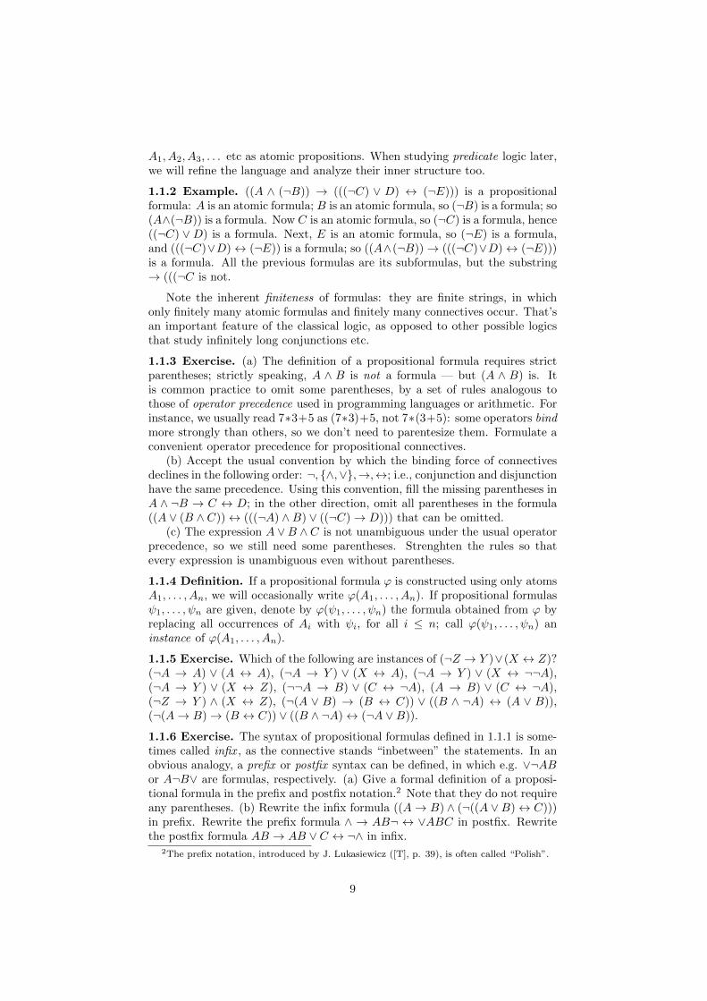
1.1.2 Example. ((A ∧ (¬B)) → (((¬C) ∨ D) ↔ (¬E))) is a propositionalformula: A is an atomic formula; B is an atomic formula, so (¬B) is a formula; so(A∧(¬B)) is a formula. Now C is an atomic formula, so (¬C) is a formula, hence((¬C) ∨D) is a formula. Next, E is an atomic formula, so (¬E) is a formula,and (((¬C)∨D)↔ (¬E)) is a formula; so ((A∧(¬B))→ (((¬C)∨D)↔ (¬E)))is a formula. All the previous formulas are its subformulas, but the substring→ (((¬C is not.

Note the inherent finiteness of formulas: they are finite strings, in whichonly finitely many atomic formulas and finitely many connectives occur. That’san important feature of the classical logic, as opposed to other possible logicsthat study infinitely long conjunctions etc.

1.1.3 Exercise. (a) The definition of a propositional formula requires strictparentheses; strictly speaking, A ∧ B is not a formula — but (A ∧ B) is. Itis common practice to omit some parentheses, by a set of rules analogous tothose of operator precedence used in programming languages or arithmetic. Forinstance, we usually read 7∗3+5 as (7∗3)+5, not 7∗(3+5): some operators bindmore strongly than others, so we don’t need to parentesize them. Formulate aconvenient operator precedence for propositional connectives.

(b) Accept the usual convention by which the binding force of connectivesdeclines in the following order: ¬, {∧,∨},→,↔; i.e., conjunction and disjunctionhave the same precedence. Using this convention, fill the missing parentheses inA ∧ ¬B → C ↔ D; in the other direction, omit all parentheses in the formula((A ∨ (B ∧ C))↔ (((¬A) ∧B) ∨ ((¬C)→ D))) that can be omitted.

(c) The expression A ∨B ∧C is not unambiguous under the usual operatorprecedence, so we still need some parentheses. Strenghten the rules so thatevery expression is unambiguous even without parentheses.

1.1.4 Definition. If a propositional formula ϕ is constructed using only atomsA1, . . . , An, we will occasionally write ϕ(A1, . . . , An). If propositional formulasψ1, . . . , ψn are given, denote by ϕ(ψ1, . . . , ψn) the formula obtained from ϕ byreplacing all occurrences of Ai with ψi, for all i ≤ n; call ϕ(ψ1, . . . , ψn) aninstance of ϕ(A1, . . . , An).

1.1.5 Exercise. Which of the following are instances of (¬Z → Y )∨(X ↔ Z)?(¬A → A) ∨ (A ↔ A), (¬A → Y ) ∨ (X ↔ A), (¬A → Y ) ∨ (X ↔ ¬¬A),(¬A → Y ) ∨ (X ↔ Z), (¬¬A → B) ∨ (C ↔ ¬A), (A → B) ∨ (C ↔ ¬A),(¬Z → Y ) ∧ (X ↔ Z), (¬(A ∨ B) → (B ↔ C)) ∨ ((B ∧ ¬A) ↔ (A ∨ B)),(¬(A→ B)→ (B ↔ C)) ∨ ((B ∧ ¬A)↔ (¬A ∨B)).

1.1.6 Exercise. The syntax of propositional formulas defined in 1.1.1 is some-times called infix , as the connective stands “inbetween” the statements. In anobvious analogy, a prefix or postfix syntax can be defined, in which e.g. ∨¬ABor A¬B∨ are formulas, respectively. (a) Give a formal definition of a proposi-tional formula in the prefix and postfix notation.2 Note that they do not requireany parentheses. (b) Rewrite the infix formula ((A→ B) ∧ (¬((A ∨B)↔ C)))in prefix. Rewrite the prefix formula ∧ → AB¬ ↔ ∨ABC in postfix. Rewritethe postfix formula AB → AB ∨ C ↔ ¬∧ in infix.

2The prefix notation, introduced by J. Lukasiewicz ([T], p. 39), is often called “Polish”.

9

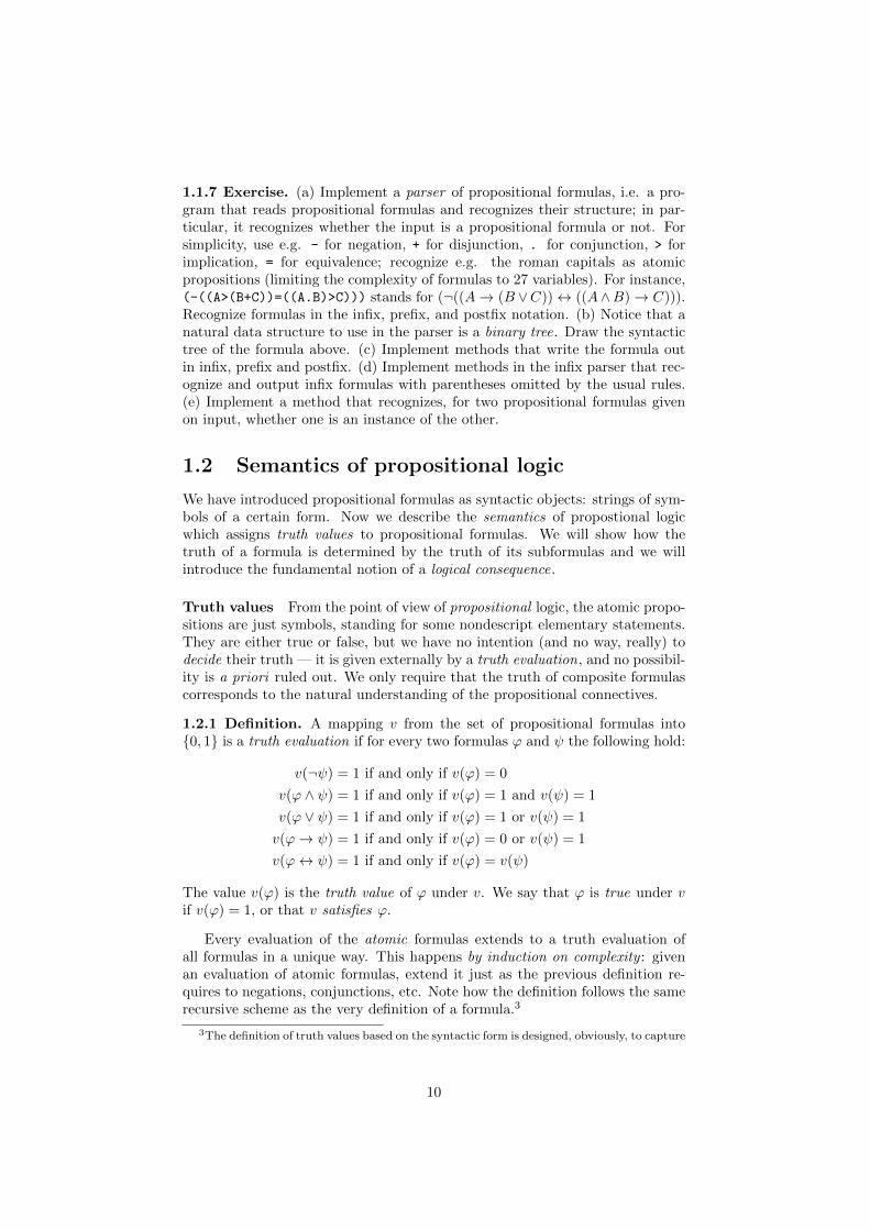
1.1.7 Exercise. (a) Implement a parser of propositional formulas, i.e. a pro-gram that reads propositional formulas and recognizes their structure; in par-ticular, it recognizes whether the input is a propositional formula or not. Forsimplicity, use e.g. - for negation, + for disjunction, . for conjunction, > forimplication, = for equivalence; recognize e.g. the roman capitals as atomicpropositions (limiting the complexity of formulas to 27 variables). For instance,(-((A>(B+C))=((A.B)>C))) stands for (¬((A→ (B ∨C))↔ ((A∧B)→ C))).Recognize formulas in the infix, prefix, and postfix notation. (b) Notice that anatural data structure to use in the parser is a binary tree. Draw the syntactictree of the formula above. (c) Implement methods that write the formula outin infix, prefix and postfix. (d) Implement methods in the infix parser that rec-ognize and output infix formulas with parentheses omitted by the usual rules.(e) Implement a method that recognizes, for two propositional formulas givenon input, whether one is an instance of the other.

1.2 Semantics of propositional logic

We have introduced propositional formulas as syntactic objects: strings of sym-bols of a certain form. Now we describe the semantics of propostional logicwhich assigns truth values to propositional formulas. We will show how thetruth of a formula is determined by the truth of its subformulas and we willintroduce the fundamental notion of a logical consequence.

Truth values From the point of view of propositional logic, the atomic propo-sitions are just symbols, standing for some nondescript elementary statements.They are either true or false, but we have no intention (and no way, really) todecide their truth — it is given externally by a truth evaluation, and no possibil-ity is a priori ruled out. We only require that the truth of composite formulascorresponds to the natural understanding of the propositional connectives.

1.2.1 Definition. A mapping v from the set of propositional formulas into{0, 1} is a truth evaluation if for every two formulas ϕ and ψ the following hold:

v(¬ψ) = 1 if and only if v(ϕ) = 0

v(ϕ ∧ ψ) = 1 if and only if v(ϕ) = 1 and v(ψ) = 1

v(ϕ ∨ ψ) = 1 if and only if v(ϕ) = 1 or v(ψ) = 1

v(ϕ→ ψ) = 1 if and only if v(ϕ) = 0 or v(ψ) = 1

v(ϕ↔ ψ) = 1 if and only if v(ϕ) = v(ψ)

The value v(ϕ) is the truth value of ϕ under v. We say that ϕ is true under vif v(ϕ) = 1, or that v satisfies ϕ.

Every evaluation of the atomic formulas extends to a truth evaluation ofall formulas in a unique way. This happens by induction on complexity : givenan evaluation of atomic formulas, extend it just as the previous definition re-quires to negations, conjunctions, etc. Note how the definition follows the samerecursive scheme as the very definition of a formula.3

3The definition of truth values based on the syntactic form is designed, obviously, to capture

10

The truth value of a formula apparently depends only on the evaluation ofthe propositional atoms that actually appear in it. We will prove this trivialstatement now, to illustrate a proof by induction on complexity .

1.2.2 Lemma. Let ϕ be a propositional formula, let A1, A2, . . . , An be thepropositional atoms occuring in ϕ. Let v and w be two evaluations agreeingon Ai, i ≤ n, i.e. v(Ai) = w(Ai) for every i ≤ n. Then v(ϕ) = w(ϕ).

Proof. (i) For an atomic formula the statement is trivial. (ii) If ϕ is of the form¬ψ and the statement holds for ψ, then v(ϕ) = v(¬ψ) = 1− v(ψ) = 1−w(ψ) =w(¬ψ) = w(ϕ). (iii) If ϕ is of the form ψ ∧ ϑ and the statement holds for ψ aϑ, then v(ϕ) = v(ψ ∧ ϑ) = 1 iff v(ψ) = 1 = v(ϑ), which is iff w(ψ) = 1 = w(ϑ),which is iff w(ψ∧ϑ) = w(ϕ) = 1. (iv) If ϕ is of the form ψ∨ϑ and the statementholds for ψ a ϑ, then v(ϕ) = v(ψ ∨ ϑ) = 1 iff v(ψ) = 1 or v(ϑ) = 1, which isiff w(ψ) = 1 or w(ϑ) = 1, which is iff w(ψ ∨ ϑ) = w(ϕ) = 1. We leave theremaining cases of (v) an implication ψ → ϑ and (vi) an equivalence ψ ↔ ϑ tothe reader.

Notice again how the recursive structure of the preceding proof correspondsto the recursive definition of a propositional formula.

Truth tables The truth values just introduced can be expressed in a compactform by the following truth table.

A B ¬A A ∧B A ∨B A→ B A↔ B0 0 1 0 0 1 10 1 1 0 1 1 01 0 0 0 1 0 01 1 0 1 1 1 1

By 1.2.2, the evaluation only depends on the evaluation of atoms occuring inthe given formula. There is only finitely many of those, as a formula is a finitestring; so there is only finitely many evaluations to consider. Hence a truthtable can be recursively compiled for any propositional formula.

1.2.3 Exercise. Compile the table of truth values for (A ∧ ¬B)→ (¬C ∨D).How many evaluations is there to consider?

1.2.4 Exercise. Show that every truth table (with 2n rows) is a truth table ofsome propositional formula (with n atoms).

1.2.5 Exercise. Implement a procedure which outputs the truth table of agiven formula. Apparently, this requires an evaluator that computes the valuesrecursively, for all possible evaluations.

A programmer will notice that we are describing certain bit operations: oninputs of 0 or 1, we return a value of 0 or 1. It is customary for some to write

the natural understanding of the connectives “and”, “or”, etc, as used in everyday language.The disjunction is used in the usual “non-exclusive” sense, so that A∨B is true if A is true orB is true, including the case when both are true. The semantics of implication is sometimescalled material implication — the truth of A → B under a given evaluation means just thatB is true if A is true; this does not mean that there is any actual cause-and-effect.

11

~A, A&B, A|B instead of ¬A, A ∧ B, A ∨ B. Introducing these operations, weimpose an algebraic structure on the set {0, 1}. In fact, we have already usedsome elementary properties of this structure, when we wrote v(¬ψ) = 1− v(ψ)for brevity in the proof of 1.2.2. We will deal with the algebraic properties oflogic when we study Boolean algebras.

Tautologies In general, the truth value of a formula depends on the evaluationof atoms. However, some formulas are special in that their truth or falsity doesin fact not depend on the evaluation.

1.2.6 Definition. A propositional formula is

(i) a contradiction if it is true under no evaluation;

(ii) satisfiable if it is true under some evaluation;

(iii) a tautology if it is true under all evaluations.

If ϕ is a tautology, we write |= ϕ.

For instance, A→ A is a tautology and B ∧ ¬B is a contradiction. A→ Bis satisfiable, but is neiter a tautology nor a contradiction. Every tautologyis satisfiable, and contradictions are precisely the non-satisfiable formulas. Anegation of a tautology is a contradiction and vice versa.

Tautologies are “always true”. We cannot expect such formulas to say any-thing specific: they are true regardless what they even talk about. The formulaA → A is always true, for any statement A, true or false. For example, thestatement if every sequence of reals converges, then any sequence of reals con-verges is surely true, but it doesn’t really say anything about convergence. It istrue simply due to its form, A→ A.

1.2.7 Exercise. Verify that the following equivalences (the deMorgan laws) aretautologies: ¬(A ∧B)↔ (¬A ∨ ¬B), ¬(A ∨B)↔ (¬A ∧ ¬B).

1.2.8 Exercise. Find out which of the following formula are tautologies, con-tradictions, and satisfiable formulas. ¬A → (A → B); A → (A → ¬A);A → (B → ¬A); ¬(A → B) → A; (A → B) ∨ (B → A); ¬A ∧ (B → A);(A↔ B) ∧ (B → ¬A); ((A→ B) ∧ (B → C) ∧ (C → D))→ (A→ D).

1.2.9 Exercise. Which of the following are tautologies? A → (B → A),(A→ (B → C))→ ((A→ B)→ (A→ C)), (¬B → ¬A)→ (A→ B).

1.2.10 Exercise. Verify that the following equivalences are tautological.¬¬A↔ A; (A∧A)↔ A; (A∨A)↔ A; (A∧B)↔ (B ∧A); (A∨B)↔ (B ∨A);(A ∧ B) ∧ C ↔ A ∧ (B ∧ C); (A ∨ B) ∨ C ↔ A ∨ (B ∨ C); A ∧ (A ∨ B) ↔ A;A∨(A∧B)↔ A; A∧(B∨C)↔ (A∧B)∨(A∧C); A∨(B∧C)↔ (A∨B)∧(A∨C);(A→ B)↔ (¬A ∨ B); A→ (B ∧ ¬B)↔ ¬A; A→ (B → C)↔ (A ∧ B)→ C;(A↔ (B ↔ C))↔ ((A↔ B)↔ C).

1.2.11 Exercise. Verify that the following formulas are tautologies.(A ∧ (A→ B))→ B, ((A→ B) ∧ ¬B)→ ¬A,(A→ B) ∧ (C → D) ∧ (A ∨ C)→ (B ∨D),(A→ B) ∧ (C → D) ∧ (¬B ∨ ¬D)→ (¬A ∨ ¬C)

12

1.2.12 Example. The truth of some formulas can be decided more effectivelythan in the general case, i.e. by checking the 2n evaluations.

(a) The formula ((A → (B → C)) → ((A → B) → (A → C))) is of a veryspecial form: it consists entirely of implications. The truth of such a formulacan be verified by considering the “worst possible case”: for an evaluation vunder which this formula is false, we necessarily have v(A → (B → C)) = 1and v((A → B) → (A → C)) = 0. hence v(A → B) = 1 and v(A → C) = 0;so v(A) = 1 and v(C) = 0; hence v(B) = 1. But under such evaluation,v(A→ (B → C)) = 0, so the whole formula is satisfied.

(b) Show that a propositional formula consisting entirely of equivalences is atautology if and only if the number of occurrences of every propositional atomis even. (Hint: the connective ↔ is commutative and associative.)

1.2.13 Definition. Let ϕ,ψ be propositional formulas. Say that ψ is a logicalconsequence of ϕ, or that ψ follows from ϕ, if every evaluation satisfying ϕ alsosatisfies ψ. In that case, write4 ϕ |= ψ. If ϕ |= ψ and ψ |= ϕ hold simultaneously,say that ϕ a ψ are logically equivalent and write ϕ |= ψ.

The basic properties of the relation of consequence are easy to see: (i) ϕ |= ψif and only if ϕ→ ψ is a tautology. (ii) ϕ |= ψ if and only if ϕ↔ ψ is a tautology.(iii) Every two tautologies — and every two contradictions — are equivalent.(iv) If ϑ is a tautology, then ϕ |= (ϕ ∧ ϑ) for every formula ϕ. (v) If ξ is acontradiction, then ϕ |= (ϕ ∨ ξ) for every formula ϕ.

1.2.14 Exercise. (a) Is the formula B∨C a consequence of (A∨B)∧(¬A∨C)?(b) Is (A→ B) ∧ (B → C) ∧ (C → A) equivalent to A↔ C?

1.2.15 Exercise. For every pair of formulas in the following sets,find out whether one is a consequence of the other, or vice versa.(a) (A ∧B)→ C, (A ∨B)→ C, (A→ C) ∧ (B → C), (A→ C) ∨ (B → C)(b) A→ (B ∧ C), A→ (B ∨ C), (A→ B) ∧ (A→ C), (A→ B) ∨ (A→ C)

1.2.16 Exercise. Let ϕ and ψ be formulas, let ϑ be a tautology, and let ξ bea contradiction. Then ϕ |= ϕ∨ ψ, ψ |= ϕ∨ ψ, ϕ∧ ψ |= ϕ, ϕ∧ ψ |= ψ, |= ξ → ϕ,|= ϕ→ ϑ, |= ϕ ∧ ϑ↔ ϕ, |= ϕ ∨ ϑ↔ ϑ, |= ϕ ∧ ξ ↔ ξ, |= ϕ ∨ ξ ↔ ϕ, |= ϑ↔ ¬ξ.

1.2.17 Exercise. Find out whether the following equivalence is a tautology,and consider the statement “The contract is valid if and only if it is written inblood or is verified by two witnesses and specifies a price and a deadline.”

((B ∨W ) ∧ (P ∧D))↔ (B ∨ (W ∧ P ∧D))

1.2.18 Exercise. How many mutually non-equivalent formulas exist over thefinite set A1, . . . , An of propositional atoms? (Hint: use 1.2.4.)

1.2.19 Exercise. Let ϕ0 and ψ0 be two logically equivalent formulas. If ϕ0 isa subformula of ϕ, and ψ is obtained from ϕ by replacing all occurrences of ϕ0

with the equivalent ψ0, then ϕ and ψ are equivalent again.

1.2.20 Example. Let ϕ be a propositional formula.

(a) If ϕ is a tautology, then every instance of ϕ is a tautology.

4For a tautology ψ, the notation |= ψ corresponds to ψ being true under any evaluation.

13

(b) If ϕ is a contradiction, then every instance of ϕ is a contradiction.

(c) If ϕ is neither a tautology nor a contradiction, then for any given truthtable there is an instance of ϕ with the prescribed truth values. (Thisstrenghtens 1.2.4.) In particular, some instance of ϕ is a tautology andsome instance of ϕ is a contradiction.

Assume that ϕ(A1, . . . , An) is neither a tautology nor a contradiction. Thenfor some evaluation f we have f(ϕ) = 0 and for some evaluation t we havet(ϕ) = 1. For every i ≤ n, choose a formula ψi(X) such that v(ψi(X)) = f(Ai)under v(X) = 0 and w(ψi(X)) = t(Ai) under w(X) = 1. Then the instanceϕ(ψ1(X), . . . , ψn(X)) of ϕ is equivalent to X. Given any truth table, choose aformula ϑ with the prescribed values, as in 1.2.4. Then ϕ(ψ1(ϑ), . . . , ψn(ϑ)) isan instance of ϕ with the prescribed table.

1.2.21 Exercise. Find an instance of A1 → (A2∨¬A3) which (i) is a tautology,(ii) is a contradiction, (iii) has the truth table 00:1, 01:0, 10:0, 11:1.

1.2.22 Exercise. Implement a procedure which for a given formula ϕ and agiven truth table finds an instance of ϕ with the prescribed truth values.

1.3 Normal form

In this section we study the expressive power of individual connectives: the lan-guage of propositional logic can be reduced in various ways, and every propo-sitional formula can be equivalently expressed in a canonical normal form. Wewill show how to find this form and how to minimize it.

The expressive power of connectives The language of propositional logicis built using the connectives ¬,∧,∨,→ and ↔. These connectives express themost needed figures of speech, and we want to capture them in the formallanguage of mathematics.

However, we have not yet tried to capture other useful figures of speech,such as the exclusive disjunction, meaning “one or the other, but not both.”This can be done with the connective A4B called XOR (exclusive or) with truthvalues of (A ∧ ¬B) ∨ (B ∧ ¬A).

It is reasonable to ask whether we should include 4 among the basic con-nectives. Such a language would surely be redundant , as 4 can be equivalentlyexpressed using the other connectives (namely by ¬,∧ and ∨; or by ¬ and↔, asA4B |= ¬A↔ B), so we can consider4 a useful shorthand, but can do withoutit. Similarly, we can consider A↔ B just a shortand for (A→ B) ∧ (B → A).

We can ask the same question about each of the connectives. A naturalrequirement for economy of language leads us to notice that some connectivescan be expressed using the others, and the language of propositional logic can bereduced . For example, all the classical connectives can be equivalently expressedusing just ¬ and ∧; indeed, (A ∨ B) ↔ ¬(¬A ∧ ¬B), (A → B) ↔ ¬(A ∧ ¬B)and (A↔ B)↔ (¬(A ∧ ¬B) ∧ ¬(B ∧ ¬A)) are tautologies.

1.3.1 Definition. A set C of connectives is complete if for any propositionalformula there is an equivalent formula using only connectives from C.

14

So we have just shown that {¬,∧} is a complete set of connectives.

1.3.2 Exercise. (a) Show that {¬,∨} and {¬,→} are complete. Reducing thelanguage of propositional logic to ¬ and → will be the first step of introducingthe formal deductive system of propositional logic later. (b) Consider a binaryconnective ⊥ (false), for which the truth value of A⊥B is 0 under all evaluations.Show that {⊥,→} is a complete set.

1.3.3 Exercise. (a) Show that A→ B cannot be equivalently expressed usingonly ¬ and ↔. So {¬,↔} is not complete. (b) Show that a propositionalformula using only ∧ and ∨ can never be a tautology or a contradiction. So{∧,∨} is not complete. (c) Show that {∧,∨,→,↔} is not complete either.

1.3.4 Exercise. An extreme case of a universal set is a universal connectiveable to express all formulas by itself. These happen to exist: A ↑ B (NAND) andA ↓ B (NOR) with truth values defined as in ¬(A∧B) and ¬(A∨B), respectively.Show that ↑ and ↓ are indeed universal. Which evaluations satisfy the formula(((((((A ↑ B) ↓ C) ↑ D) ↓ E) ↑ F ) ↓ G) ↑ H)?

1.3.5 Lemma. ↑ and ↓ are the only universal connectives.

Proof. Let A � B be a universal connective. Then under u(A) = 1 = u(B) wemust have u(A �B) = 0, for if u(A �B) = 1, then every formula built from A,Busing only � would have a value of 1 under u (which is easily seen by induction);but then � could not be universal. Similarly, under v(A) = 0 = v(B) we havev(A � B) = 1. Notice that the universal connectives ↑ and ↓ indeed have thisproperty. It remains to check the value of A � B under w(A) = 0, w(B) = 1and z(A) = 1, z(B) = 0. Considering the four possibilities, we see that A � Bbehaves either as A ↑ B or A ↓ B and we are done, or as ¬A or ¬B, which areeasily seen not to be universal.

As a corollary, we obtain that the universal sets {¬,∧}, {¬,∨}, {¬,→},{⊥,→} from above are also minimal , i.e. they cannot be further reduced.

1.3.6 Exercise. Implement a procedure which translates a given formula intoan equivalent formula in a given minimal universal set of connectives.

1.3.7 Exercise. After introducing XOR, NAND and NOR, we can ask what exactlydo we consider a connective. Abstractly, a binary connective is a mapping from{0, 1} × {0, 1} to {0, 1}. Hence there is as many “connectives” as there are

mappings from 22 to 2, i.e. 222

= 16. Compile the truth table of all 16 binaryconnectives and decribe them using the connectives introduced so far.

Normal form

1.3.8 Definition. A propositional formula is

(i) a literal if it is an atomic formula or a negation of an atomic formula;

(ii) a minterm if it is a conjunction of literals;

(iii) a maxterm or a clause if it is a dijunction of literals;

(iv) in a disjunctive normal form (DNF) if it is a disjunction of minterms;

15

(v) in a conjunctive normal form (CNF) if it is a conjunction of maxterms;

(vi) in a complete normal form if all minterms/maxterms use the same atoms.

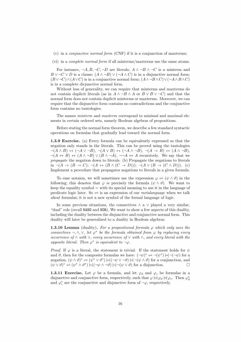
For instance, ¬A,B,¬C,¬D are literals; A ∧ ¬B ∧ ¬C is a minterm andB ∨ ¬C ∨D is a clause; (A ∧ ¬B) ∨ (¬A ∧ C) is in a disjunctive normal form;(B∨¬C)∧ (A∨C) is in a conjunctive normal form; (A∧¬B∧C)∨ (¬A∧B∧C)is in a complete dicjunctive normal form.

Without loss of generality, we can require that minterms and maxterms donot contain duplicit literals (as in A ∧ ¬B ∧ A or B ∨ B ∨ ¬C) and that thenormal form does not contain duplicit minterms or maxterms. Moreover, we canrequire that the disjunctive form contains no contradictions and the conjunctiveform contains no tautologies.

The names minterm and maxterm correspond to minimal and maximal ele-ments in certain ordered sets, namely Boolean algebras of propositions.

Before stating the normal form theorem, we describe a few standard syntacticoperations on formulas that gradually lead toward the normal form.

1.3.9 Exercise. (a) Every formula can be equivalently expressed so that thenegation only stands in the literals. This can be proved using the tautologies¬(A ∧ B) ↔ (¬A ∨ ¬B), ¬(A ∨ B) ↔ (¬A ∧ ¬B), ¬(A → B) ↔ (A ∧ ¬B),¬(A ↔ B) ↔ (A ∧ ¬B) ∨ (B ∧ ¬A), ¬¬A ↔ A recursively. We say that wepropagate the negation down to literals. (b) Propagate the negations to literalsin ¬(A → (B → C); ¬(A ↔ (B ∧ (C → D))); ¬(A ∨ (B → (C ∧ D))). (c)Implement a procedure that propagates negations to literals in a given formula.

To ease notaion, we will sometimes use the expression ϕ (ψ ∧ ϑ) in thefollowing; this denotes that ϕ is precisely the formula (ψ ∧ ϑ). We want tokeep the equality symbol = with its special meaning to use it in the language ofpredicate logic later. So is an expression of our metalanguage when we talkabout formulas; it is not a new symbol of the formal language of logic.

In some previous situations, the connectives ∧ a ∨ played a very similar,“dual” role (recall NAND and NOR). We want to show a few aspects of this duality,including the duality between the disjunctive and conjunctive normal form. Thisduality will later be generalized to a duality in Boolean algebras.

1.3.10 Lemma (duality). For a propositional formula ϕ which only uses theconnectives ¬,∧,∨, let ϕ∗ be the formula obtained from ϕ by replacing everyoccurrence of ∧ with ∨, every occurrence of ∨ with ∧, and every literal with theopposite literal. Then ϕ∗ is equivalent to ¬ϕ.

Proof. If ϕ is a literal, the statement is trivial. If the statement holds for ψand ϑ, then for the composite formulas we have: (¬ψ)∗ ¬(ψ∗) |= ¬(¬ψ) for anegation, (ψ ∧ ϑ)∗ (ψ∗ ∨ ϑ∗) |= (¬ψ ∨ ¬ϑ) |= ¬(ψ ∧ ϑ) for a conjunction, and(ψ ∨ ϑ)∗ (ψ∗ ∧ ϑ∗) |= (¬ψ ∧ ¬ϑ) |= ¬(ψ ∨ ϑ) for a disjunction.

1.3.11 Exercise. Let ϕ be a formula, and let ϕd and ϕc be formulas in adisjunctive and conjunctive form, respectively, such that ϕ |= ϕd |= ϕc. Then ϕ∗dand ϕ∗c are the conjunctive and disjunctive form of ¬ϕ, respectively.

16

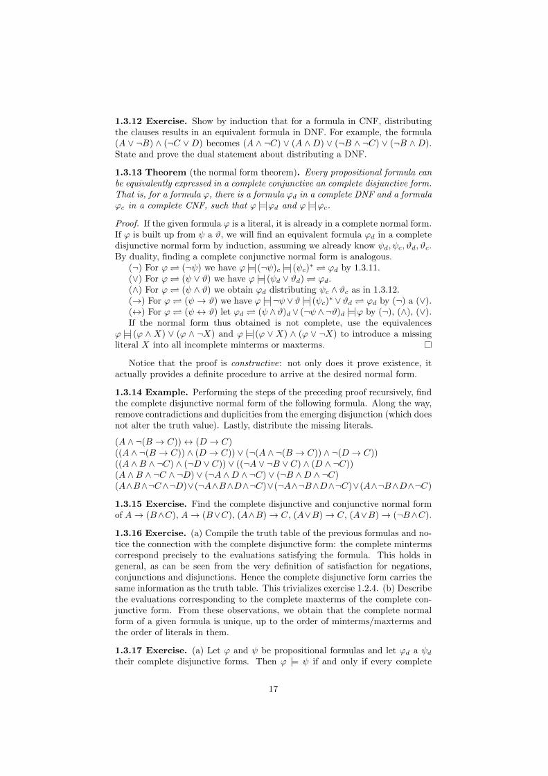
1.3.12 Exercise. Show by induction that for a formula in CNF, distributingthe clauses results in an equivalent formula in DNF. For example, the formula(A ∨ ¬B) ∧ (¬C ∨D) becomes (A ∧ ¬C) ∨ (A ∧D) ∨ (¬B ∧ ¬C) ∨ (¬B ∧D).State and prove the dual statement about distributing a DNF.

1.3.13 Theorem (the normal form theorem). Every propositional formula canbe equivalently expressed in a complete conjunctive an complete disjunctive form.That is, for a formula ϕ, there is a formula ϕd in a complete DNF and a formulaϕc in a complete CNF, such that ϕ |= ϕd and ϕ |= ϕc.

Proof. If the given formula ϕ is a literal, it is already in a complete normal form.If ϕ is built up from ψ a ϑ, we will find an equivalent formula ϕd in a completedisjunctive normal form by induction, assuming we already know ψd, ψc, ϑd, ϑc.By duality, finding a complete conjunctive normal form is analogous.

(¬) For ϕ (¬ψ) we have ϕ |= (¬ψ)c |= (ψc)∗ ϕd by 1.3.11.

(∨) For ϕ (ψ ∨ ϑ) we have ϕ |= (ψd ∨ ϑd) ϕd.(∧) For ϕ (ψ ∧ ϑ) we obtain ϕd distributing ψc ∧ ϑc as in 1.3.12.(→) For ϕ (ψ → ϑ) we have ϕ |= ¬ψ ∨ϑ |= (ψc)

∗ ∨ϑd ϕd by (¬) a (∨).(↔) For ϕ (ψ ↔ ϑ) let ϕd (ψ ∧ ϑ)d ∨ (¬ψ ∧¬ϑ)d |= ϕ by (¬), (∧), (∨).If the normal form thus obtained is not complete, use the equivalences

ϕ |= (ϕ ∧ X) ∨ (ϕ ∧ ¬X) and ϕ |= (ϕ ∨ X) ∧ (ϕ ∨ ¬X) to introduce a missingliteral X into all incomplete minterms or maxterms.

Notice that the proof is constructive: not only does it prove existence, itactually provides a definite procedure to arrive at the desired normal form.

1.3.14 Example. Performing the steps of the preceding proof recursively, findthe complete disjunctive normal form of the following formula. Along the way,remove contradictions and duplicities from the emerging disjunction (which doesnot alter the truth value). Lastly, distribute the missing literals.

(A ∧ ¬(B → C))↔ (D → C)((A ∧ ¬(B → C)) ∧ (D → C)) ∨ (¬(A ∧ ¬(B → C)) ∧ ¬(D → C))((A ∧B ∧ ¬C) ∧ (¬D ∨ C)) ∨ ((¬A ∨ ¬B ∨ C) ∧ (D ∧ ¬C))(A ∧B ∧ ¬C ∧ ¬D) ∨ (¬A ∧D ∧ ¬C) ∨ (¬B ∧D ∧ ¬C)(A∧B∧¬C∧¬D)∨(¬A∧B∧D∧¬C)∨(¬A∧¬B∧D∧¬C)∨(A∧¬B∧D∧¬C)

1.3.15 Exercise. Find the complete disjunctive and conjunctive normal formof A→ (B∧C), A→ (B∨C), (A∧B)→ C, (A∨B)→ C, (A∨B)→ (¬B∧C).

1.3.16 Exercise. (a) Compile the truth table of the previous formulas and no-tice the connection with the complete disjunctive form: the complete mintermscorrespond precisely to the evaluations satisfying the formula. This holds ingeneral, as can be seen from the very definition of satisfaction for negations,conjunctions and disjunctions. Hence the complete disjunctive form carries thesame information as the truth table. This trivializes exercise 1.2.4. (b) Describethe evaluations corresponding to the complete maxterms of the complete con-junctive form. From these observations, we obtain that the complete normalform of a given formula is unique, up to the order of minterms/maxterms andthe order of literals in them.

1.3.17 Exercise. (a) Let ϕ and ψ be propositional formulas and let ϕd a ψd

their complete disjunctive forms. Then ϕ |= ψ if and only if every complete

17

minterm of ϕd is also a complete minterm of ψd. State the dual statement forconjunctive normal forms. (b) Find the complete DNF of ¬((A∨B)→ ¬C) anddecide whether it is a consequence of ¬(A→ (B ∨¬C)). (c) Find the completeCNF of A → (¬B ∧ C) and decide whether the formula B → (A → C) is itsconsequence. (d) Find the DNF of (A → (D ∨ ¬E)) → (C ∧ ¬(A → B)) anddecide whether it is a consequence of (¬(E → D)) ∧A.

1.3.18 Exercise. Is there a formula ϕ such that both ϕ→ (A∧B) and (ϕ∨¬A)are tautologies? (Hint: what is the complete DNF of such a formula?)

1.3.19 Exercise. Give the missing dual half of the proof of 1.3.13, i.e. describehow to arrive at the conjunctive normal form, by induction on complexity.

1.3.20 Exercise. Implement a procedure that rewrites a given formula into itscomplete conjunctive/disjunctive normal form.

Minimization We have described a way to arrive at the complete normalform. Now we will describe a method of finding a minimal normal form, whichcan be useful in applications.

1.3.21 Example. The following formula is in a complete disjunctive form:

(A∧¬B ∧¬C)∨ (¬A∧¬B ∧¬C)∨ (A∧B ∧C)∨ (A∧B ∧¬C)∨ (¬A∧B ∧¬C)

It is natural to ask whether it can be written in a shorter normal form, and whatis the shortest normal form possible. Notice that some pairs of the completeminterms differ in precisely one literal, e.g. (A∧¬B∧¬C) and (¬A∧¬B∧¬C).Using the distributivity law, every such pair can be equivalently replaced withone shorter minterm; in this case, (¬B∧¬C). Similarly, the complete minterms(A ∧ B ∧ ¬C) ∨ (¬A ∧ B ∧ ¬C) can be replaced with (B ∧ ¬C). Now theminterms (¬B∧¬C)∨(B∧¬C) can be merged to ¬C, and the formula becomes(A ∧B) ∨ ¬C. This is a DNF where nothing can be merged anymore.

There is more than one way to merge the minterms with opposite literals:pairing the first two via A,¬A and the second two via C,¬C, we get

(¬B ∧ ¬C) ∨ (A ∧B) ∨ (¬A ∧B ∧ ¬C)

which cannot be further simplified either, but the one above is shorter: twominterms instead of three, and fewer literals in each. So the choice of mergingthe minterms can make a difference.

1.3.22 Example ([Sha]). A switching circuit can be described by a diagramwhere every switch is annotated with a necessary and sufficient condition forthe current to flow. For example, the current flows through

A B

C

¬BA

18

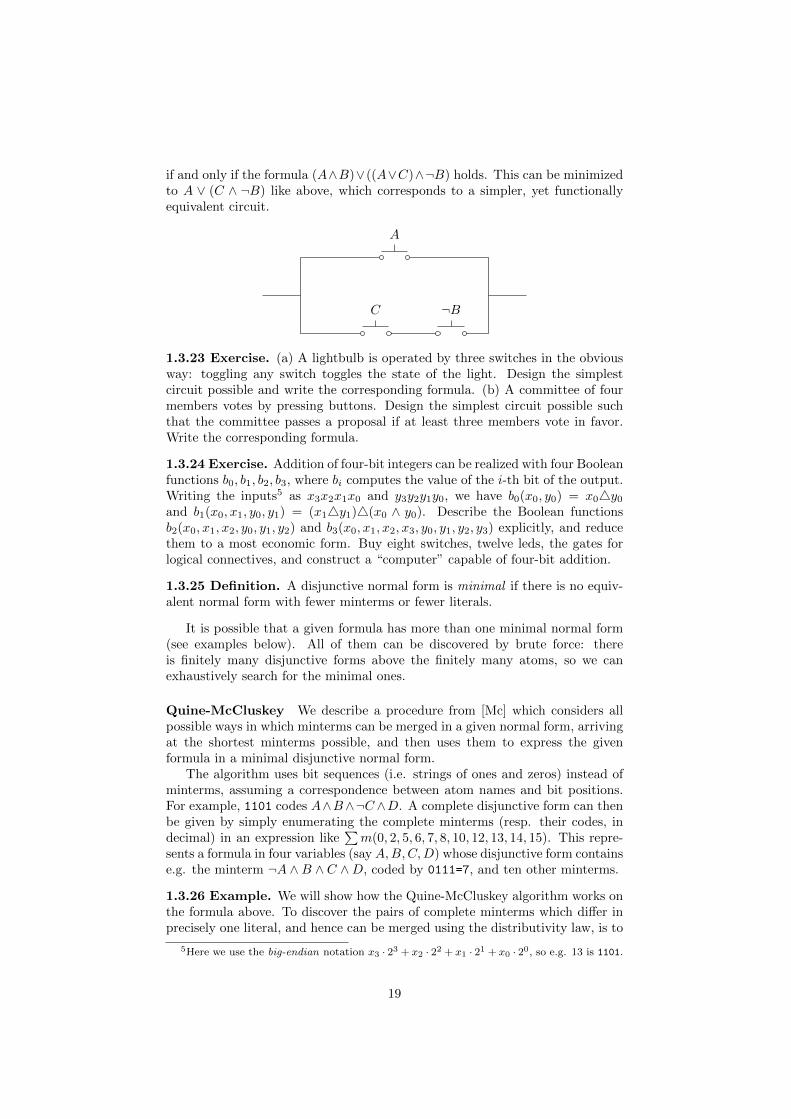
if and only if the formula (A∧B)∨((A∨C)∧¬B) holds. This can be minimizedto A ∨ (C ∧ ¬B) like above, which corresponds to a simpler, yet functionallyequivalent circuit.

A

C ¬B

1.3.23 Exercise. (a) A lightbulb is operated by three switches in the obviousway: toggling any switch toggles the state of the light. Design the simplestcircuit possible and write the corresponding formula. (b) A committee of fourmembers votes by pressing buttons. Design the simplest circuit possible suchthat the committee passes a proposal if at least three members vote in favor.Write the corresponding formula.

1.3.24 Exercise. Addition of four-bit integers can be realized with four Booleanfunctions b0, b1, b2, b3, where bi computes the value of the i-th bit of the output.Writing the inputs5 as x3x2x1x0 and y3y2y1y0, we have b0(x0, y0) = x04y0and b1(x0, x1, y0, y1) = (x14y1)4(x0 ∧ y0). Describe the Boolean functionsb2(x0, x1, x2, y0, y1, y2) and b3(x0, x1, x2, x3, y0, y1, y2, y3) explicitly, and reducethem to a most economic form. Buy eight switches, twelve leds, the gates forlogical connectives, and construct a “computer” capable of four-bit addition.

1.3.25 Definition. A disjunctive normal form is minimal if there is no equiv-alent normal form with fewer minterms or fewer literals.

It is possible that a given formula has more than one minimal normal form(see examples below). All of them can be discovered by brute force: thereis finitely many disjunctive forms above the finitely many atoms, so we canexhaustively search for the minimal ones.

Quine-McCluskey We describe a procedure from [Mc] which considers allpossible ways in which minterms can be merged in a given normal form, arrivingat the shortest minterms possible, and then uses them to express the givenformula in a minimal disjunctive normal form.

The algorithm uses bit sequences (i.e. strings of ones and zeros) instead ofminterms, assuming a correspondence between atom names and bit positions.For example, 1101 codes A∧B∧¬C∧D. A complete disjunctive form can thenbe given by simply enumerating the complete minterms (resp. their codes, indecimal) in an expression like

∑m(0, 2, 5, 6, 7, 8, 10, 12, 13, 14, 15). This repre-

sents a formula in four variables (say A,B,C,D) whose disjunctive form containse.g. the minterm ¬A ∧B ∧ C ∧D, coded by 0111=7, and ten other minterms.

1.3.26 Example. We will show how the Quine-McCluskey algorithm works onthe formula above. To discover the pairs of complete minterms which differ inprecisely one literal, and hence can be merged using the distributivity law, is to

5Here we use the big-endian notation x3 · 23 + x2 · 22 + x1 · 21 + x0 · 20, so e.g. 13 is 1101.

19

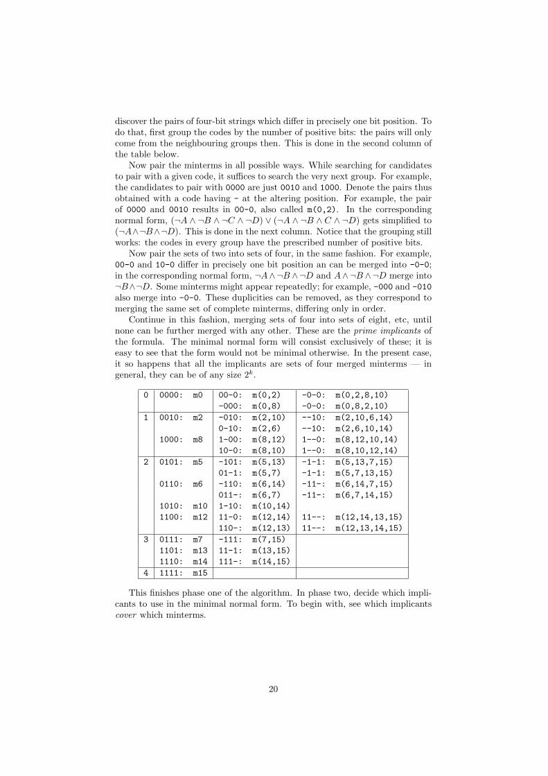
discover the pairs of four-bit strings which differ in precisely one bit position. Todo that, first group the codes by the number of positive bits: the pairs will onlycome from the neighbouring groups then. This is done in the second column ofthe table below.

Now pair the minterms in all possible ways. While searching for candidatesto pair with a given code, it suffices to search the very next group. For example,the candidates to pair with 0000 are just 0010 and 1000. Denote the pairs thusobtained with a code having - at the altering position. For example, the pairof 0000 and 0010 results in 00-0, also called m(0,2). In the correspondingnormal form, (¬A ∧ ¬B ∧ ¬C ∧ ¬D) ∨ (¬A ∧ ¬B ∧ C ∧ ¬D) gets simplified to(¬A∧¬B∧¬D). This is done in the next column. Notice that the grouping stillworks: the codes in every group have the prescribed number of positive bits.

Now pair the sets of two into sets of four, in the same fashion. For example,00-0 and 10-0 differ in precisely one bit position an can be merged into -0-0;in the corresponding normal form, ¬A∧¬B ∧¬D and A∧¬B ∧¬D merge into¬B∧¬D. Some minterms might appear repeatedly; for example, -000 and -010

also merge into -0-0. These duplicities can be removed, as they correspond tomerging the same set of complete minterms, differing only in order.

Continue in this fashion, merging sets of four into sets of eight, etc, untilnone can be further merged with any other. These are the prime implicants ofthe formula. The minimal normal form will consist exclusively of these; it iseasy to see that the form would not be minimal otherwise. In the present case,it so happens that all the implicants are sets of four merged minterms — ingeneral, they can be of any size 2k.

0 0000: m0 00-0: m(0,2) -0-0: m(0,2,8,10)

-000: m(0,8) -0-0: m(0,8,2,10)

1 0010: m2 -010: m(2,10) --10: m(2,10,6,14)

0-10: m(2,6) --10: m(2,6,10,14)

1000: m8 1-00: m(8,12) 1--0: m(8,12,10,14)

10-0: m(8,10) 1--0: m(8,10,12,14)

2 0101: m5 -101: m(5,13) -1-1: m(5,13,7,15)

01-1: m(5,7) -1-1: m(5,7,13,15)

0110: m6 -110: m(6,14) -11-: m(6,14,7,15)

011-: m(6,7) -11-: m(6,7,14,15)

1010: m10 1-10: m(10,14)

1100: m12 11-0: m(12,14) 11--: m(12,14,13,15)

110-: m(12,13) 11--: m(12,13,14,15)

3 0111: m7 -111: m(7,15)

1101: m13 11-1: m(13,15)

1110: m14 111-: m(14,15)

4 1111: m15

This finishes phase one of the algorithm. In phase two, decide which impli-cants to use in the minimal normal form. To begin with, see which implicantscover which minterms.

20

0 2 5 6 7 8 10 12 13 14 15

-0-0: m(0,2,8,10) * * * *

--10: m(2,6,10,14) * * * *

1--0: m(8,10,12,14) * * * *

-1-1: m(5,7,13,15) * * * *

-11-: m(6,7,14,15) * * * *

11--: m(12,13,14,15) * * * *

Some minterms are only covered by one implicant; for example, 0=0000 isonly covered by m(0,2,8,10), and m(5,7,13,15) is the only implicant covering5=0101. These are the esential implicants: they must be present in the minimalform. In the original language, this means the minimal form will necessarilycontain the minterms (¬B ∧ ¬D) and (B ∧D). The essential implicants coverm(0,2,5,7,8,10,13,15). It remains to find a minimal cover of the rest.

6 12 14

--10: m(2,6,10,14) * *

1--0: m(8,10,12,14) * *

-11-: m(6,7,14,15) * *

11--: m(12,13,14,15) * *

These coverings are not mutually independent: every implicant covering 6

or 12 also covers 14. This is minterm dominance. Hence 14 can be ignored andit only remains to cover 6 and 12.

6 12

--10: m(2,6,10,14) *

1--0: m(8,10,12,14) *

-11-: m(6,7,14,15) *

11--: m(12,13,14,15) *

Now each of the remaining minterms covered by m(2,6,10,14) is also cov-ered by m(6,7,14,15), and vice versa. The same relation holds for the impli-cants m(8,10,12,14) and m(12,13,14,15). This is implicant dominance. Itsuffices to choose one from each; choose the first from each, for instance.

6 12

--10: m(2,6,10,14) *

1--0: m(8,10,12,14) *

After these reductions, all implicants become essential for a cover of theremaining minterms. These are the secondary essentials. The correspondingminimal normal form is then

(¬B ∧ ¬D) ∨ (B ∧D) ∨ (C ∧ ¬D) ∨ (A ∧ ¬D).

In the extreme case when all primary implicats are essential, the minimalform is uniquely determined. Generally, as in the present case, it depends onthe covering choices. Any of the following is also a minimal normal form.

(¬B ∧ ¬D) ∨ (B ∧D) ∨ (C ∧ ¬D) ∨ (A ∧B)

(¬B ∧ ¬D) ∨ (B ∧D) ∨ (B ∧ C) ∨ (A ∧ ¬D)

(¬B ∧ ¬D) ∨ (B ∧D) ∨ (B ∧ C) ∨ (A ∧B)

21

1.3.27 Exercise. Add 4=0100 (i.e. ¬A∧B∧¬C ∧¬D) to the disjunctive formabove, perform the QMC algorithm, and see how the minimal form changes.

1.3.28 Exercise. Implement the Quine-McCluskey algorithm.

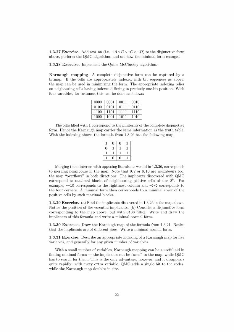
Karnaugh mapping A complete disjunctive form can be captured by abitmap. If the cells are appropriately indexed with bit sequences as above,the map can be used in minimizing the form. The appropriate indexing relieson neigbouring cells having indexes differing in precisely one bit position. Withfour variables, for instance, this can be done as follows:

0000 0001 0011 00100100 0101 0111 01101100 1101 1111 11101000 1001 1011 1010

The cells filled with 1 correspond to the minterms of the complete disjunctiveform. Hence the Karnaugh map carries the same information as the truth table.With the indexing above, the formula from 1.3.26 has the following map.

1 0 0 10 1 1 11 1 1 11 0 0 1

Merging the minterms with opposing literals, as we did in 1.3.26, correspondsto merging neighbours in the map. Note that 0, 2 or 8, 10 are neighbours too:the map “overflows” in both directions. The implicants discovered with QMCcorrespond to maximal blocks of neighbouring pisitive cells of size 2k. Forexample, --10 corresponds to the rightmost column and -0-0 corresponds tothe four corners. A minimal form then corresponds to a minimal cover of thepositive cells by such maximal blocks.

1.3.29 Exercise. (a) Find the implicants discovered in 1.3.26 in the map above.Notice the position of the essential implicants. (b) Consider a disjunctive formcorresponding to the map above, but with 0100 filled. Write and draw theimplicants of this formula and write a minimal normal form.

1.3.30 Exercise. Draw the Karnaugh map of the formula from 1.3.21. Noticethat the implicants are of different sizes. Write a minimal normal form.

1.3.31 Exercise. Describe an appropriate indexing of a Karnaugh map for fivevariables, and generally for any given number of variables.

With a small number of variables, Karnaugh mapping can be a useful aid infinding minimal forms — the implicants can be “seen” in the map, while QMChas to search for them. This is the only advantage, however, and it disappearsquite rapidly: with every extra variable, QMC adds a single bit to the codes,while the Karnaugh map doubles in size.

22

1.4 Satisfiability

In this section, we deal with satisfiability of propositional formulas and propo-sitional theories. The question of satisfiability of formulas is a link betweenmathematical logic and complexity theory via the well-known SAT Problem.We describe the resolution method which effectively decides the satisfiability offinite propositional theories, and prove the compactness theorem which dealswith satisfiability of infinite theories.

SAT Problem Compiling a truth table is an effective procedure deciding sat-isfiability of a propositional formula. However, for a formula with n variables,there are 2n evaluations to consider, so the method of truth tables is not partic-ularly effective: the complexity of computation grows exponentially in relationto the size of input. It is natural to ask whether there is a more effective way.

The problem of deciding satisfiability of any given propositional formula isknown as SAT , and an algorithm solving this problem is a SAT solver . Sofar, we have described two: compiling the truth table and finding the completenormal form. Now we ask how complex a SAT solver needs to be.

The focus is shifted now: while the solvability of SAT is trivial from the pointof view of logic, the complexity of a solution is interesting for computer science.It is proven in [Co] that SAT is NP-complete. The NP class of complexity con-sists of problems that can be solved in polynomial time with a non-deterministicTuring machine.6 Cook’s theorem says that every such problem can be reducedto SAT, with a deterministic machine in polynomial time. A solution to SATthan yields a solution to the original problem. Hence SAT itself must be com-putationally very hard: at least as hard as any problem from NP.

In fact, [Co] proves more: SAT is NP-complete even in the case when theinput formulas are presented in a disjunctive form, and moreover none of theminterms contains more than three literals.

The P class of complexity consists of the problems which can be solved inpolynomial time with a deterministic Turing machine. As a consequence ofCook’s theorem, we get that if there is a deterministic polynomial SAT solver(i.e. if SAT is in P), then a deterministic polynomial solution also exists for allproblems from NP, and so P = NP . The question whether P = NP is knownas the PNP Problem, and is widely considered to be one of the most importantopen questions of computer science. By Cook’s theorem, the question can bereduced to the existence of a deterministic polynomial SAT solver.

Resolution We generalize the basic notions of propositional logic form for-mulas to sets of formulas, i.e. propositional theories, and describe an algorithmthat decides the satisfiability of finite theories. This is a SAT solver, because tosatisfy a finite theory ϕ1, . . . , ϕn is to satisfy the formula ϕ1 ∧ . . . ∧ ϕn.

1.4.1 Definition. Any set of propositional formulas is a propositional theory ,and its members are its axioms. A propositional theory T is satisfied under anevaluation v, if v satisfies every axiom in T . A theory is satisfiable if there is anevaluation satisfying it.

6See [Mo] for an introduction into Turing machines and computability in general.

23

1.4.2 Definition. Lat T be a propositional theory and let ϕ be a propositionalformula. Say that ϕ follows from T , or that it is a consequence of T , and writeT |= ϕ, if every evaluation satisfying T also satisfies ϕ. More generally, if S andT are propositional theories, say that T follows from S, and write S |= T , ifevery evaluation satisfying S also satisfies T . If both S |= T and T |= S holdsimultaneously, say that S and T are equivalent , and write S |= T .

If T is a propositional theory and ϕ is a formula, then T |= ϕ if and only ifT ∪ {¬ϕ} is not satisfiable. Two theories S and T are equivalent if and only iffor every formula ϕ we have T |= ϕ iff S |= ϕ. In other words, two theories areequivalent if they have the same consequences.

1.4.3 Exercise. Are {A∨¬B,C∨¬A,A} and {C,B → C,A∨¬C} equivalent?Are {A ∨B,¬A ∨ C} and {A→ C,B ∨ C} equivalent?

The resolution method extends a given porpositional theory into an equiv-alent theory R(T ) whose satisfiability can be decided trivially. We know hatevery formula, and so every finite theory as well, can be expressed in a con-junctive normal form. Hence without loss of generality, we can view any givenproositional theory as a set of clauses, and the clauses as sets of literals.

If (A ∨ B1 ∨ . . . ∨ Bn) and (¬A ∨ C1 ∨ . . . ∨ Cm) are two clauses, then(B1 ∨ . . . ∨Bn ∨ C1 ∨ . . . ∨ Cm) is their reslovent . The resolvent can be empty,e.g. A a ¬A have an empty resolvent; we will denote an empty resolvent as ⊥and call it a contradiction, as usual. Is is easy to see that the resolvent is aconsequence of the two clauses.

1.4.4 Lemma. Every truth evaluation satisfying clauses (A ∨ B1 ∨ . . . ∨ Bn)and (¬A ∨ C1 ∨ . . . ∨ Cm) also satisfies (B1 ∨ . . . ∨Bn ∨ C1 ∨ . . . ∨ Cm).

If T is a finite set of clauses, denote by r(T ) the union of T with the set ofall possible resolvents of clauses from T . Clearly T ⊆ r(T ), and if T is finite,r(T ) is finite too. The theories T and r(T ) are equivalent, as all the clauses inr(T ) are consequences of T .

Put r0(T ) = T and rn+1(T ) = r(rn(T )). Then T = r0(T ) ⊆ r1(T ) ⊆ . . . ⊆rn(T ) ⊆ rn+1(T ) ⊆ . . . is an increasing chain of finite theories. As there areonly finitely many clauses using the finitely many literals from T , and resolutiondoes not introduce new literals, the increasing chain must stabilize at some finitestep, i.e. rn(T ) = rn+1(T ) for some n ∈ N. We will call this set of clauses theresolution closure of T and denote it by R(T ).

1.4.5 Example. The resolution closure of T = {A ∨ B,B → C,C → D,D →E} grow by the following contributions to the rn(T ):

r0: A ∨B,¬B ∨ C,¬C ∨D,¬D ∨ Er1: A ∨ C,¬B ∨D,¬C ∨ Er2: A ∨D,¬B ∨ E,A ∨ E

Checking all pairs of clauses systematically, it is easy to check that there areno other resolvents. The resoltion closure has stabilized after two iterations.

The theories T , r(T ) and R(T ) are equivalent. In particular, T is satisfi-able iff R(T ) is satisfiable. Now we can formulate the theorem that makes theresolution method work.

1.4.6 Theorem (J. Herbrand). A finite set T of clauses is satisfiable if andonly if its resolution closure R(T ) does not contain a contradiction.

24

Proof. One direction is immediate: if R(T ) contains a contradiction, it is notsatisfiable, and neither is the equivalent theory T . In the other direction, weshow that R(T ) is satisfiable, provided it does not contain a contradiction.

Let A1, . . . , Ak be the language of T , i.e. the atoms occurring in the clausesfrom T . By induction, we define an evaluation v of these atoms which satisfiesR(T ). If Aj is the first atom not yet evaluated, define v(Aj) as follows: if thereis a clause in R(T ) which consists exclusively of ¬Aj and literals evaluatedinversely to the evaluation so far, put v(Aj) = 0; otherwise, put v(Aj) = 1.

If ϕ is a clause form R(T ) not satisfied by v, then ϕ consists exclusively ofliterals evaluated inversely to v; in that case, let j ≤ k be the first possible indexsuch that all atoms occurring in some such ϕ are among A1, . . . , Aj . This doesnot necessarily mean that all of them occur in ϕ, but the atom Aj must occur,or the chosen j was not the first possible. We check the case when ϕ containsthe literal Aj — the opposite case when ϕ contains ¬Aj is analogous.

So we have v(Aj) = 0, otherwise ϕ is satisfied. Hence by the definitionof v, there is some clause ψ in R(T ) consisting exclusively of ¬Aj and literalsevaluated inversely to A1, . . . , Aj−1. The atom Aj must occur in ψ, otherwisej was not the first possible; so ψ contains ¬Aj . But then the resolvent of ϕand ψ, a member of R(T ), consists exclusively of literals evaluated inversely toAj , . . . , Aj−1. This contradicts the minimality of the chosen j ≤ k. The onlyremaining possibility is that the resolution is empty, i.e. a contradiction. ButR(T ) does not contain a contradiction.

1.4.7 Example. Is {P ∧Q→ R,¬R∧P,¬Q∨¬R} satisfiable? The resolutionstabilizes without reaching a contradiction, and moreover ¬Q is among theresolvents, so P,¬Q,¬R is the only satisfying evaluation.

1.4.8 Exercise. (a) Is the formula (¬B ∧ ¬D)→ (¬A ∧ ¬E) a consequence of{A→ (B∨C), E → (C ∨D),¬C}? Checking truth tables means considering 25

evaluations of four different formulas. Denote the formula as ϕ and the theoryas T and ask instead whether T,¬ϕ is satisfiable. (b) It is natural to alsoask whether the theory T is itself satisfiable, because if not, any formula is itsconsequence. Check the satisfiability of T .

1.4.9 Exercise. Check {B∧D → E,B∧C → F,E∨F → A,¬C → D,B} |= Aand {B ∧D → E,B ∧ C → F,E ∨ F → A,C → D,B} |= A.

1.4.10 Exercise. The Law and Peace political party needs to get their ministerout of a corruption case. This requires either to intimmidate witness A or tobribe judge B. To intimmidate A, person C needs to be jailed. To bribe judgeB, the company F must be overtaken and given contract E. Jailing C andovertaking F require killing person D. Does Law and Peace need to kill D?

1.4.11 Exercise. Implement the resolution method as a program which trans-lates a given finite theory into a set of clauses, generates all resolvents, andeither stops at a contradiction or stabilizes at a satisfiable resolution closure,obtaining a satisfying evaluation as in 1.4.6.

Compactness Satisfiability of a finite propositional theory is not really differ-ent from satisfiability of a formula. We discuss now the interesting case: infinitetheories. We prove the compactness theorem for propositional logic, which is in

25

fact a principle inherent in all mathematics based on set theory. We show twoapplications of compactness: colouring graphs and linearizing orders.

1.4.12 Exercise. (a) In the language of {An;n ∈ N}, consider the infinite theo-ries S = {¬An ↔ An+2;n ∈ N} and T = {¬An ↔ (An+1 ∨An+2);n ∈ N}. De-cide whether they are satisfiable, and if so, describe the satisfying evaluations.(b) Show that neither of the theories S and T follows from the other. (c) Foran infinite theory T , it is natural to ask whether there is a finite fragmentT0 ⊂ T such that T |= T0. The satisfiability of T could then be reduce to thesatisfiability of T0. Show that S and T above have no equivalent finite part.

1.4.13 Theorem (compactness of propositional logic). A propositional theoryis satisfiable if and only if every finite fragment is satisfiable.

The theorem is only interesting for infinite theories, and one direction isimmediate: an evaluation satisfying the theory also satisfies every fragment —the strength is in the opposite direction.

We present two proofs of the compactness theorem. Firstly, we assume thelanguage of the theory to be countable, which makes it possible to build thesatisfying evaluation by induction. In the proof, we use the notion of a finitelysatisfiable theory , which is a theory whose every finite part can be satisfied. Weare to show that such a theory is, in fact, satisfiable.

1.4.14 Lemma. Let T be a finitely satisfiable theory, let ϕ be a formula. Theneither T ∪ {ϕ} or T ∪ {¬ϕ} is also finitely satisfiable.

Proof. If not, then some finite parts T0∪{ϕ} ⊆ T∪{ϕ} and T1∪{¬ϕ} ⊆ T∪{¬ϕ}are not satisfiable. But then T0 ∪ T1 ⊆ T is a non-satisfiable fragment of T : anevaluation satisfying T0 ∪ T1 could satisfy neither ϕ nor ¬ϕ.

Proof of the compactness theorem. Let T be a finitely satisfiable propositionaltheory. Assume that the language of T is countable, and enumerate all7 propo-sitional formulas as {ϕn;n ∈ N}.

We construct by induction a propositional theory U extending T . Startwith U0 = T . If a finitely satisfiable theory Un is known, let Un+1 be either thefinitely satisfiable Un ∪ {ϕn} or the finitely satisfiable Un ∪ {¬ϕn}; one of thesemust be the case, by the previous lemma. Finaly, put U =

⋃Un.

Notice that U is finitely satisfiable: a finite part of U is a finite part of someUn already. Moreover, the following holds for any formulas ϕ and ψ:

(i) ¬ϕ ∈ U iff ϕ /∈ U . Both cannot be the case, as U is finitely satisfiable.The formula ϕ is one of the ϕn, so either ϕ ∈ Un+1 or ¬ϕ ∈ Un+1 at the latest.

(ii) ϕ ∧ ψ ∈ U iff ϕ,ψ ∈ U . For if ϕ ∧ ψ ∈ U but ϕ /∈ U or ψ /∈ U , then¬ϕ ∈ U or ¬ψ ∈ U by (i), so either {¬ϕ,ϕ∧ψ} or {¬ψ,ϕ∧ψ} is a non-satisfiablefinite part of U . Conversely, if ϕ,ψ ∈ U but ϕ ∧ ψ /∈ U , then ¬(ϕ ∧ ψ) ∈ U by(i), and {ϕ,ψ,¬(ϕ ∧ ψ)} is a non-satisfiable finite part of U .

(iii) ϕ ∨ ψ ∈ U iff ϕ ∈ U or ψ ∈ U . For if (ϕ ∨ ψ) ∈ U but ϕ,ψ /∈ U , then¬ϕ,¬ψ ∈ U by (i), and {ϕ ∨ ψ,¬ϕ,¬ψ} is a non-satisfiable finite part of U .Similarly in the other direction.

(iv) ϕ → ψ ∈ U iff either ¬ϕ ∈ U or ψ ∈ U . For if ϕ → ψ ∈ U but¬ϕ,ψ /∈ U , then ϕ,¬ψ ∈ U by (i) and {ϕ,ϕ→ ψ,¬ψ} is a non-satisfiable finitepart of U . Similarly in the other direction.

7Note that we enumerate all formulas, not just those in T .

26

(v) ϕ ↔ ψ ∈ U iff either ϕ,ψ ∈ U or ϕ,ψ /∈ U . For if ϕ ↔ ψ ∈ U but e.g.ϕ ∈ U and ψ /∈ U , then ¬ψ ∈ U by (i) and {ϕ ↔ ψ,ϕ,¬ψ} is a non-satisfiablefinite part of U . Similarly in the other direction.

Now let v(ϕ) = 1 iff ϕ ∈ U . The properties above say precisely that vis a truth evaluation. Clearly v satisfies all formulas from U , in particular allformulas from T ⊆ U . Hence T is satisfiable.

It remains to prove the theorem for a language A of arbitrary cardinality. Wepresent a general proof, which needs a few notions from set-theoretical topology.

Proof of the compactness theorem. Let T be a finitely satisfiable theory. Forevery finite fragment S ⊆ T denote by sat(S) the set of all evaluations v : A → 2satisfying S. By assumption, sat(S) is nonempty for every finite S ⊆ T . Itis easily seen that sat(S) is closed in the topological product 2A. The systemS = {sat(S);S ⊆ T finite} is centered, as the intersection sat(S1)∩· · ·∩sat(Sn)contains the nonempty sat(S1 ∪ · · · ∪ Sn). Hence we have a centered system Sof nonempty closed sets in 2A, which is a compact topological space, so theintersection

⋂S is nonempty. Every evaluation v ∈

⋂S 6= ∅ satisfies all finite

S ⊆ T simultaneously; in particular, it satisfies every formula from T .

Notice that the above proof is purely existential : we have shown that asatisfying evaluation exists, without presenting any particular one.

1.4.15 Lemma. Let T be a propositional theory T and ϕ be a propositionalformula. Then T |= ϕ if and only if T0 |= ϕ for some finite T0 ⊆ T .

Proof. T |= ϕ iff T ∪{¬ϕ} is not satisfiable, which by the compactness theoremmeans that T0 ∪ {¬ϕ} is not satisfiable for some finite T0 ⊆ T . So T0 |= ϕ.

1.4.16 Lemma. Let T be a propositional theory, and let S be a finite proposi-tional theory such that S |= T . Then there is a finite T0 ⊆ T such that T0 |= T .

Proof. For every formula ϕ from S, we have T |= ϕ by assumption. By theprevious lemma, there is a finite Tϕ ⊆ T such that Tϕ |= ϕ. Put T0 =

⋃ϕ∈S Tϕ.

Being a finite union of finite sets, T0 is a finite part of T ; in particular, T |= T0.Clearly T0 |= S, and by assumption, S |= T ; hence T0 |= T .

For example, the propositional theories from 1.4.12 have no equivalent finitefragment. By the lemma just proven, they have no finite equivalent at all.

1.5 Provability

So far, we have been concerned with the semantics of propositional logic, askingquestions of truth, satisfiability and consequence. Now we describe the otherface of propositional logic, the formal deductive system. We introduce the notionof a formal proof and ask which formulas are provable, either in logic alone orfrom other formulas. We demonstrate the deduction theorem which considerablysimplifies and shortens provability arguments. We demonstrate the completenessof propositional logic, showing the notions of truth and provability in accord.

27

A formal deductive system When proposing a deductive system for propo-sitional logic, we first need to specify the language it will use. In this language,certain formulas are chosen as axioms from which everything else will be derived,and a set of deductive rules is explicitly given which are the only permitted waysof deriving anything. It is almost philosophical to ask what the axioms and therules should be, and different formal systems answer this question differently.The system introduced by D. Hilbert is widely recognized as the standard.

The Hilbert system The language of the Hilbert deductive system is thelanguage of propositional logic reduced to the connectives ¬ and →. The pur-pose of this reduction is an economy of expression; we know from 1.3.2 that{¬,→} is a minimal complete set of connectives. The axioms are all instancesof any of the following formulas:

H1: A→ (B → A)

H2: (A→ (B → C))→ ((A→ B)→ (A→ C))

H3: (¬B → ¬A)→ (A→ B)

The only deductive rule is the rule of detachment or modus ponens:

MP: From ϕ and ϕ→ ψ, derive ψ.

Do H1–H3 constitute the right foundation upon which the provability ofpropositions should stand, and does MP truly capture the way reason progressesfrom the known to the new? We will not be concerned with these questions here,leaving them to the philosophy of mathematics.

1.5.1 Exercise. Note that there are not just three axioms, but infinitely manyaxioms of three types. (a) Which of the following formulas are axioms, andof which type? (b) Implement a procedure which recognizes if a given inputformula is a Hilbert axiom, and of which type.

(A → B) → ((¬C ↔ (D ∧ E)) → (A → B))

(A → B) → ((¬C ↔ (D ∧ E)) → (A → (A ∨B)))

(A → ((B ∧ ¬C) → D)) → ((A → (B ∧ ¬C)) → (A → D))

(A → ((B ∧ ¬C) → D)) → ((A → (B ∧ ¬C)) → D)

(¬(A ∧B) → (C ∨D)) → (¬(C ∨D) → (A ∧B))

(¬(A ∧B) → ¬¬(C ∨D)) → (¬(C ∨D) → (A ∧B))

1.5.2 Definition. Let ϕ be a propositional formula. Say that a finite sequenceϕ1, . . . , ϕn of propositional formulas is a proof of ϕ in propositional logic, ifevery ϕi from the sequence is either an instance of an axiom, or is derived fromsome previous ϕj , ϕk, j, k < i by modus ponens, and ϕn is ϕ. If a proof of ϕexists, say that ϕ is provable and write ` ϕ.

The notion of a proof captures what we expect from it in mathematics:starting from explicitly given assumptions, it proceeds by explicitely given rules,and is verifiable in each of its finitely many steps. This verification can even bemechanical, see 1.5.6.

1.5.3 Example. The following sequence is a formal proof of A→ A in propo-sitional logic. In every step, we note which axiom or rule exactly is being used.

28

H1: (A → ((A → A) → A))

H2: (A → ((A → A) → A)) → ((A → (A → A)) → (A → A))

MP: (A → (A → A)) → (A → A)

H1: (A → (A → A))

MP: (A → A)

Note that the notion of a proof is entirely syntactic: it is a sequence offormulas, i.e. expressions of certain form, which itself is of certain form. Thequestions of truth or satisfaction are entirely irrelevant here.

It is easy to verify that the sequence above is indeed a proof, but it gives nohint about how to find a proof. We will see later that for a provable formula, evenfinding the proof is a mechanical procedure, although very hard computationally.

Introducing formal proofs, a note of warning is in order: we also present“proofs” in this text, and they are not sequences of formulas (except 1.5.3).To clearly separate these two levels of a language, we could call our proofsdemonstrations or metaproofs, as is sometimes done. However, we keep callingthem “proofs” and rely on the reader’s ability to differentiate between a formalproof in logic and a demonstration given in English, which is the metalanguagewe use to talk about logic, i.e. about formulas, theories — and proofs.

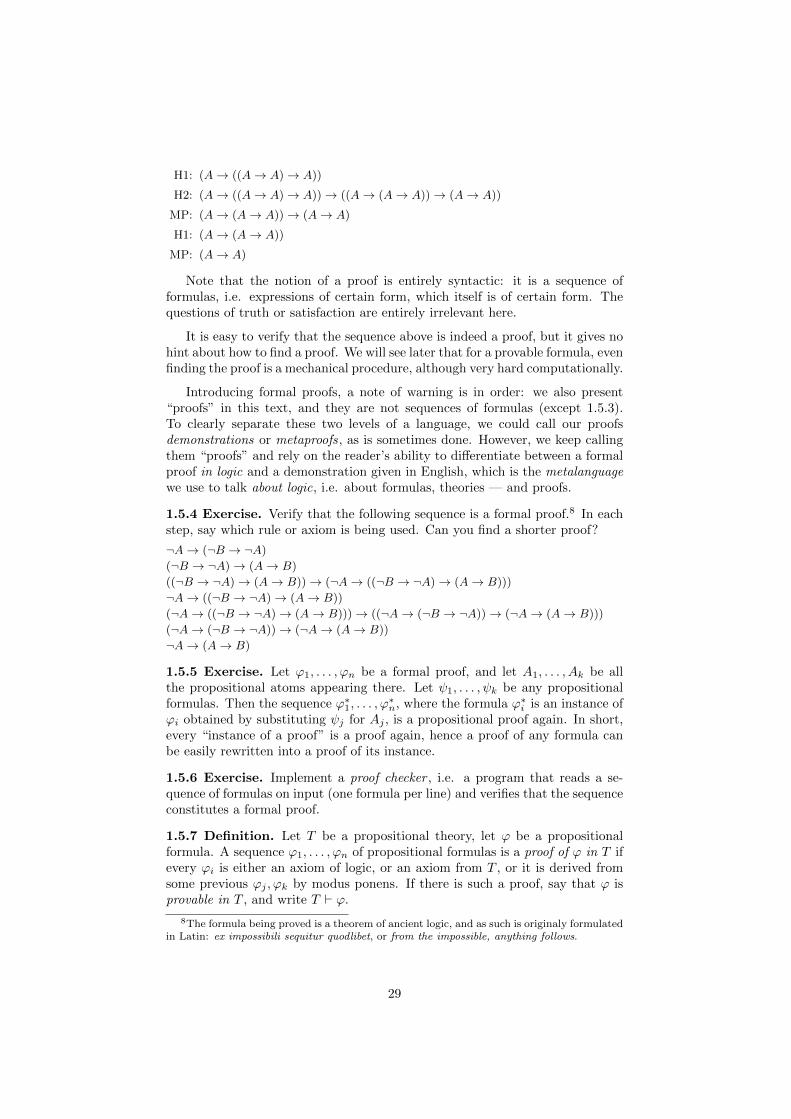
1.5.4 Exercise. Verify that the following sequence is a formal proof.8 In eachstep, say which rule or axiom is being used. Can you find a shorter proof?

¬A → (¬B → ¬A)

(¬B → ¬A) → (A → B)

((¬B → ¬A) → (A → B)) → (¬A → ((¬B → ¬A) → (A → B)))

¬A → ((¬B → ¬A) → (A → B))

(¬A → ((¬B → ¬A) → (A → B))) → ((¬A → (¬B → ¬A)) → (¬A → (A → B)))

(¬A → (¬B → ¬A)) → (¬A → (A → B))

¬A → (A → B)

1.5.5 Exercise. Let ϕ1, . . . , ϕn be a formal proof, and let A1, . . . , Ak be allthe propositional atoms appearing there. Let ψ1, . . . , ψk be any propositionalformulas. Then the sequence ϕ∗1, . . . , ϕ

∗n, where the formula ϕ∗i is an instance of

ϕi obtained by substituting ψj for Aj , is a propositional proof again. In short,every “instance of a proof” is a proof again, hence a proof of any formula canbe easily rewritten into a proof of its instance.

1.5.6 Exercise. Implement a proof checker , i.e. a program that reads a se-quence of formulas on input (one formula per line) and verifies that the sequenceconstitutes a formal proof.

1.5.7 Definition. Let T be a propositional theory, let ϕ be a propositionalformula. A sequence ϕ1, . . . , ϕn of propositional formulas is a proof of ϕ in T ifevery ϕi is either an axiom of logic, or an axiom from T , or it is derived fromsome previous ϕj , ϕk by modus ponens. If there is such a proof, say that ϕ isprovable in T , and write T ` ϕ.

8The formula being proved is a theorem of ancient logic, and as such is originaly formulatedin Latin: ex impossibili sequitur quodlibet, or from the impossible, anything follows.

29

The generalization is in that we allow formulas from T as steps of the proof.The notation ` ϕ introduced before corresponds to the case when ϕ is provablein an empty theory, i.e. in logic alone.

If the theory in question is finite, it is usual to simply list its axioms. Forexample, we write B,¬A→ ¬B ` A instead of {B,¬A→ ¬B} ` A (see below).Similarly, if a theory T is extended with extra axioms ϕ and ψ, it is usual towrite shortly T, ϕ, ψ instead of T ∪ {ϕ,ψ} etc.

1.5.8 Exercise. (a) Verify the steps of a formal proof of A→ B from ¬A: ¬A,¬A→ (¬B → ¬A), ¬B → ¬A, (¬B → ¬A)→ (A→ B), A→ B.(b) Give a proof of A→ B from B and a proof of A from B,¬A→ ¬B.

1.5.9 Exercise ([T]). For a propositional theory T , denote by Thm(T ) the setof formulas provable in T . Decide which the following hold:

(a) T ⊆ Thm(T )

(b) Thm(Thm(T )) = Thm(T )

(c) S ⊆ T if and only if Thm(S) ⊆ Thm(T )

(d) S ⊆ Thm(T ) if and only if Thm(S) ⊆ Thm(T )

(e) Thm(S ∪ T ) = Thm(S) ∪ Thm(T )

(f) Thm(S ∪ T ) = Thm(S ∪ Thm(T )) = Thm(Thm(S) ∪ Thm(T ))

(g) If Tn ⊆ Tn+1 for every n ∈ N, then Thm(⋃Tn) =

⋃Thm(Tn)

(h) If Tn is a directed system, then Thm(⋃Tn) =

⋃Thm(Tn)

Correctness and consistence Having introduced formal proofs, it is naturalto ask which formulas are provable, in logic or in a given theory. We show firstthat the Hilbert system is correct and propositional logic is therefore consistent .

1.5.10 Theorem (correctness). Let T be a propositional theory and let ϕ be apropositional formula. If ϕ is provable in T , then ϕ is a logical consequence ofT . In particular, porpositional logic itself only proves tautologies.

Proof. Let ϕ1, ϕ2, . . . , ϕn be a proof of ϕ in T . If ϕi is an axiom of propositionallogic, it is a tautology, as we have verified in 1.2.9 and 1.2.20, so T |= ϕi. If ϕi

is a member of T , then T |= ϕi by definition. Finally, if ϕi is derived for someprevious two by modus ponens, note that an evaluation satisfying % and %→ ϑalso satisfies ϑ; hence modus ponens only derives tautologies from tautologies,and only derives consequences of T from consequences of T .

1.5.11 Definition. A propositional theory is inconsistent if it proves everyformula; otherwise, it is consistent . A formal system itself is inconsistent if theempty theory is inconsistent.

Hence by the correctness theorem, propositional logic is consistent : a formulawhich is not a tautology cannot be proven. We also get from correctness that

1.5.12 Theorem. Every satisfiable theory is consistent.

30

Proof. Let v be an evaluation satisfying T . If T is inconsistemt, it proves any for-mula, in particular some ϕ and ¬ϕ, simultaneously. By the correctness theorem,T |= ϕ and T |= ¬ϕ. Hence v satisfies both ϕ and ¬ϕ, which is impossible.

The property that an inconsistent theory proves both ϕ and ¬ϕ, for someformula ϕ, does in fact characterize the inconsistent theories, and is sometimestaken as the definition. For if ψ is any formula, we have ` ¬ϕ → (ϕ → ψ) by1.5.4, so if T ` ϕ and T ` ¬ϕ, use modus ponens twice to get T ` ψ.

Deduction theorem We present an indispensable technical tool: the deduc-tion theorem, which simplifies and shortens proofs. We use it to show provabilityof some simple formulas needed later.

1.5.13 Theorem (deduction). Let T be a propositional theory, let ϕ,ψ be propo-sitional formulas. Then T ` ϕ→ ψ if and only if T, ϕ ` ψ.

The deduction theorem formalizes the usual technique of proving an impli-cation ϕ → ψ: the assumption ϕ is added to the theory, and the conclusion ψis proved. Such a proof is typically shorter, as we are proving a simpler formulafrom stronger assumptions. In 1.5.4, for instance, we have given a formal proofof ¬ϕ→ (ϕ→ ψ) in propositional logic, in seven steps. In 1.5.8 we have provedϕ→ ψ from ¬ϕ in five notably easier steps.

Proof. (i) If T ` ϕ → ψ, let ϑ1, ϑ2, . . . , ϑn (ϕ → ψ) be a proof. Extend thissequence by ϕ,ψ, obtaining ϑ1, ϑ2, . . . , (ϕ→ ψ), ϕ, ψ, a proof of ψ form T, ϕ.

(ii) If T, ϕ ` ψ, let ϑ1, ϑ2, . . . , ϑn ψ be a proof of ψ in T, ϕ. By induction,we show that T ` ϕ→ ϑi for every ϑi. In particular, T ` ϕ→ ψ for i = n.

(a) If ϑi is an axiom, then ϑi, ϑi → (ϕ→ ϑi), ϕ→ ϑi is a proof of ϕ→ ϑi.(b) If ϑi is from T , then the sequence from (a) is a proof of ϕ→ ϑi from T .(c) If ϑi ϕ, we need to show T ` ϕ→ ϕ. But ` ϕ→ ϕ by 1.5.3.(d) If ϑi is derived from some previous ϑj , ϑj → ϑi using modus ponens, we

already have T ` ϕ → ϑj and T ` ϕ → (ϑj → ϑi). A proof of ϕ → ϑi in T isthen obtained by extending the proofs of ϕ→ ϑj and ϕ→ (ϑj → ϑi) by

H2: (ϕ → (ϑj → ϑi)) → ((ϕ → ϑj) → (ϕ → ϑi))

MP: (ϕ → ϑj) → (ϕ → ϑi)

MP: ϕ → ϑi

This covers all cases of ϑi being in the original proof.

The demonstration is constructive: it describes an algorithm which trans-lates a proof of ψ from T, ϕ into a proof of ϕ→ ψ from T , and vice versa.

1.5.14 Example. We show how to rewrite the proof 1.5.8 of A→ B from ¬Ainto a proof of ¬A→ (A→ B) in logic. We follow the constructive demonstra-tion of the deduction theorem: for each of the formulas ϑ1, ϑ2, ϑ3, ϑ4, ϑ5, i.e¬A, ¬A → (¬B → ¬A), ¬B → ¬A, (¬B → ¬A) → (A → B), A → B of theoriginal proof, we construct a proof of ¬A→ ϑi.

(1) ϑ1 is ¬A itself, case 1.5.13 (c), using 1.5.3:

(¬A → ((¬A → ¬A) → ¬A))

(¬A → ((¬A → ¬A) → ¬A)) → ((¬A → (¬A → ¬A)) → (¬A → ¬A))

(¬A → (¬A → ¬A)) → (¬A → ¬A)

31

(¬A → (¬A → ¬A))

(¬A → ¬A)

(2) ϑ2 is an axiom of logic, case 1.5.13 (a):

¬A → (¬B → ¬A)

(¬A → (¬B → ¬A)) → (¬A → (¬A → (¬B → ¬A)))

¬A → (¬A → (¬B → ¬A))

(3) ϑ3 was derived from ϑ1 and ϑ2, case 1.5.13 (d):

(¬A → (¬A → (¬B → ¬A))) → ((¬A → ¬A) → (¬A → (¬B → ¬A)))

(¬A → ¬A) → (¬A → (¬B → ¬A))

¬A → (¬B → ¬A)

(4) ϑ4 is an axiom of logic, case 1.5.13 (a):

(¬B → ¬A) → (A → B)

((¬B → ¬A) → (A → B)) → (¬A → ((¬B → ¬A) → (A → B)))

¬A → ((¬B → ¬A) → (A → B))

(5) ϑ5 was derived from ϑ3 and ϑ4, case 1.5.13 (d):

(¬A → ((¬B → ¬A) → (A → B))) → ((¬A → (¬B → ¬A)) → (¬A → (A → B)))

(¬A → (¬B → ¬A)) → (¬A → (A → B))

¬A → (A → B)

Apparently, formal proofs of even simple formulas can get quite tedious.9

The deduction theorem makes it possible to keep provability arguments tolerablysimple. At the same time, the use of the deduction theorem can always beeliminated as above, mechanically.

1.5.15 Exercise. Demonstrate that (A → (B → C)) → (B → (A → C)) and(A → B) → ((B → C) → (A → C)) are provable. The deduction theoremmakes it possible to show provability without actually giving a formal proof .

1.5.16 Exercise. Extend your proof checker to a proof preprocessor whichaccepts provability arguments like above and unfolds every use of the deductiontheorem into an actual formal proof.

We will be using the deduction theorem freely when showing provability ofvarious propositional formulas below. The gentle reader can try and see howmuch more tedious it would be to present the actual formal proofs.

1.5.17 Lemma. (i) ` ¬¬A→ A, (ii) ` A→ ¬¬A.

Proof. Using 1.5.4 and the deduction theorem, we have

1.5.4: ` ¬¬A → (¬A → ¬¬¬A)

DT: ¬¬A ` (¬A → ¬¬¬A)

H3: ` (¬A → ¬¬¬A) → (¬¬A → A)

MP: ¬¬A ` ¬¬A → A

DT: ¬¬A ` A

DT: ` ¬¬A → A

9The formal proof obtained above can in fact be simplified: the first eleven steps prove aninstance of an axiom, which, moreover, is already present as the sixth step. Eliminating theredundancies leads to the proof in 1.5.4.

32

and

(i) ` ¬¬¬A → ¬AH3: ` (¬¬¬A → ¬A) → (A → ¬¬A)

MP: ` A → ¬¬A

1.5.18 Lemma. (i) ` (A→ B)→ (¬B → ¬A), (ii) ` A→ (¬B → ¬(A→ B))

Proof. Using 1.5.17 and the deduction theorem, we have

1.5.17, DT: ¬¬A ` A

MP: ¬¬A,A → B ` B

1.5.17, MP: ¬¬A,A → B ` ¬¬BDT: A → B ` ¬¬A → ¬¬B

H3, MP: A → B ` ¬B → ¬BDT: ` (A → B) → (¬B → ¬B)

and

MP: A,A → B ` B

DT: A ` (A → B) → B

(i), MP: A ` ¬B → ¬(A → B)

DT: ` A → (¬B → ¬(A → B))

1.5.19 Lemma. ` (¬A→ A)→ A.

Proof. Using 1.5.18 and the deduction theorem, we have

MP: ¬A,¬A → A ` A

DT: ¬A ` (¬A → A) → A

1.5.18, MP: ¬A ` ¬A → ¬(¬A → A)

DT, DT: ` ¬A → ¬(¬A → A)

H3, MP: ` (¬A → A) → A

1.5.20 Exercise. ` (A→ ¬B)→ (B → ¬A), ` (¬A→ B)→ (¬B → A).

Using the previous lemmas, we obtain the following characterization of prov-ability. This can be viewed as a formalization of a proof by contradiction.

1.5.21 Lemma. T ` ϕ if and only if T,¬ϕ is inconsistent.

Proof. (i) By 1.5.4 we have ` ¬ϕ → (ϕ → ψ), so ` ϕ → (¬ϕ → ψ) by 1.5.15.Hence if T ` ϕ, then T ` ¬ϕ→ ψ, and so T,¬ϕ ` ψ by the deduction theorem.

(ii) If T,¬ϕ is inconsistent, it proves any formula, in particular T,¬ϕ ` ϕ,and we have T ` ¬ϕ→ ϕ by the deduction theorem. Now ` (¬ϕ→ ϕ)→ ϕ by1.5.19, hence T ` ϕ by modus ponens.

These provability results are only concerned with the connectives ¬ and →;we show now some simple proofs of formulas concerning the other connectives,taking them as shortcuts for equivalents in the basic language.

33

1.5.22 Lemma. (i) A ∧B ` A,B, (ii) A,B ` A ∧B.

Proof. (i) A ∧ B stands for ¬(A → ¬B). By 1.5.4 we have ¬A → (A → B),so by 1.5.17 and 1.5.18 we have ` ¬(A → ¬B) → A by modus ponens. Hence¬(A → ¬B) ` A by the deduction theorem. Also, ¬B → (A → ¬B) is anaxiom, hence 1.5.17 and 1.5.18 give ` ¬(A → ¬B) → B by modus ponens, so¬(A→ ¬B) ` B by the deduction theorem. (ii) We have A,B ` ¬¬B by 1.5.17,so by 1.5.18 A,¬¬B ` ¬(A→ ¬B). Hence A,B ` A∧B by modus ponens.

1.5.23 Lemma. A↔ B standing for (A→ B) ∧ (B → A), we have

(i) A↔ B ` A→ B; A↔ B ` B → A

(ii) A→ B,B → A ` A↔ B

(iii) If ` A↔ B, then T ` A iff T ` B.

(iv) ` (A1 → (A2 → . . . (An → B) . . . )↔ ((A1 ∧A2 . . . ∧An)→ B)

1.5.24 Exercise. (i) A ` A∧A, (ii) A ` A∨A, (iii) A∧A ` A, (iv) A∨A ` A.

Completeness of propositional logic We show now the completeness ofthe Hilbert system: it proves exactly the tautologies. This means that the setof axioms and rules of inference fully characterize the truth of propositionalformulas by entirely formal, syntactic means.

1.5.25 Lemma (neutral formula). Let T be a propositional theory and let ϕ,ψbe propositional formulas. If T, ϕ ` ψ and T,¬ϕ ` ψ, then T ` ψ.

Proof. From T,¬ϕ ` ψ we have T ` ¬ψ → ¬¬ϕ by 1.5.18, so T,¬ψ ` ¬¬ϕby the deduction theorem, and T,¬ψ ` ϕ by 1.5.17. From T, ϕ ` ψ we haveT ` ϕ → ψ by the deduction theorem, so T,¬ψ ` ψ by modus ponens, andT ` ¬ψ → ψ. By 1.5.19 we have ` (¬ψ → ψ)→ ψ, so T ` ψ.

For a propositional formula ϕ and a truth evaluation v, let ϕv denote eitherϕ, in case v(ϕ) = 1, or ¬ϕ, in case v(ϕ) = 0. In any case, v(ϕv) = 1.

1.5.26 Lemma. Let ϕ be a propositional formula and let A1, . . . , An be itspropositional atoms. Then Av

1, . . . , Avn ` ϕv for any evaluation.

Proof. If ϕ is an atom itself, the statement is trivial. If ϕ is ¬ψ and the statementis already proved for ψ, consider two cases. For v(ψ) = 0, the formula ψv is ¬ψ,and by induction Av

1, . . . , Avn ` ¬ψ; but ¬ψ is ϕv. For v(ψ) = 1, the formula ψv

is ψ, and by induction Av1, . . . , A

vn ` ψ. By 1.5.17 we have ` ψ → ¬¬ψ, hence

Av1, . . . , A

vn ` ¬¬ψ by modus ponens; but ¬¬ψ is ϕv.

If ϕ is ψ → ϑ and the statement is already proved for ψ and ϑ, consider thecases of v(ψ) and v(ϑ). If v(ψ) = 0, ψv is ¬ψ and ϕv is ψ → ϑ. By 1.5.4 and thededuction theorem we have ¬ψ ` ψ → ϑ, so the statement follows by induction.In case v(ψ) = 1 = v(ϑ), we have v(ϕ) = 1, so ϕv is ψ → ϑ. By H1 and thededuction theorem we have ϑ ` ψ → ϑ; but ϑ is ϑv, so the statement followsby induction. In case v(ψ) = 1, v(ϑ) = 0 we have v(ϕ) = 0, so ϕv is ¬ϕ, i.e.¬(ψ → ϑ). By 1.5.18 and the deduction theorem we have ψ,¬ϑ ` ¬(ψ → ϑ);but ψ is ψv and ¬ϑ is ϑv, so the statement follows by induction.

34

1.5.27 Theorem (E. Post). Every propositional tautology is provable.

Proof. Let ϕ be a tautology, and let A1, . . . , An be its propositional atoms. Forevery evaluation v we have Av

1, . . . , Avn ` ϕ by the previous lemma. Let w be an

evaluation which agrees with v everywhere except An. We have Aw1 , . . . , A

wn ` ϕ

again, i.e. Av1, A

v2, . . . , A

vn−1, A

wn ` ϕ. Hence we have

Av1, A

v2, . . . , A

vn−1, An ` ϕ

Av1, A

v2, . . . , A

vn−1,¬An ` ϕ

simultaneously and Av1, . . . , A

vn−1 ` ϕ by 1.5.25. Repeat n times to get ` ϕ.

1.5.28 Theorem (completeness of propositional logic). Let ϕ be a propositionalformula and T a propositional theory. Then T ` ϕ iff T |= ϕ. In particular,propositional logic itself proves exactly the tautologies.

Proof. One direction is the corectess theorem. In the other direction, let T |= ϕ.By the compactness theorem, we already have T0 |= ϕ for some finite partT0 = {ϕ1, . . . , ϕn} of T . This means that ϕ1 → (ϕ2 → . . . (ϕn → ϕ) . . . ) is atautology, and is provable in propositional logic by Post’s theorem. Using thededuction theorem n times, we get ϕ1, . . . , ϕn ` ϕ, hence T ` ϕ.

We have demonstrated the correspondence between truth and provability inpropositional logic. This has interesting corollaries and equivalents.

1.5.29 Theorem. A propositional theory is consistent iff it is satisfiable.

Proof. One direction is 1.5.12. If T is not satisfiable, then by compactness somefinite {ϕ1, . . . , ϕn} ⊆ T is not satisfiable. Hence ¬ϕ1 ∨ . . .∨¬ϕn is a tautology,denote it by ϕ. By the completeness theorem, ϕ is provable in logic, so T ` ϕas well. At the same time, every ϕi is provable in T , hence T ` ϕ1 ∧ . . . ∧ ϕn

by 1.5.22. But this formula is equivalent to ¬ϕ, so T ` ¬ϕ by 1.5.23.

In the demonstration we use the compactness theorem, which itself followsfrom the previous theorem. For if T is not satisfiable, it is inconsistent. But theformal proof of a contradiction in T only uses a finite part T0 ⊆ T , as a proofis a finite sequence. So the finite T0 is inconsistent, hence not satisfiable.

The completeness theorem itself also follows from the previous theorem. Forif T |= ϕ, then T,¬ϕ is not satisfiable, and is therefore inconsistent. Hence somefinite part T0,¬ϕ is inconsistent, which means T0 ` ϕ by 1.5.21.

Decidability of propositional logic The question of provability for propo-sitional formulas is, by the completeness theorem, the same as the question oftruth. Yet the truth of a propositional formula can be effectively decided, hencethere is a procedure effectively deciding provability of any given propositionalformula. We say that propositional logic is decidable.

In the next chapter, we study predicate logic, which also has a completenesstheorem, but is undecidable. In predicate logic, there is no analogy of the truthtables which could effectively decide the truth of formulas.

35

Chapter 2

Predicate Logic

The language of propositional connectives is hardly fine enough to be the lan-guage of mathematics. In this chapter, we study the language in more detail,introducing the functional and relational symbols used in mathematics to de-scribe objects and their properties, and study its syntax and semantics. Weextend the Hilbert axioms and rules of inference to these new symbols anddescribe the deductive system of predicate logic, which has become the formalframework of mathematics. We prove the corectness and completeness theorem,and show the compactness of predicate logic.

2.1 Formulas of predicate logic

In propositional logic, we have studied the connectives and how they operate onthe atomic statements, ignoring the inner structure of these statements. Nowwe study this structure in detail.

When studying the formal language of mathematics, designed to describemathematical structures, we must ask first what the language is supposed toexpress. Surely we want to name some particular objects, for instance. Thelanguage of predicate logic contains constant symbols for this. For example,the symbols 0 and 1 in arithmetic or π in real analysis are names for someprominent numbers, the constants sin or exp name certain functions, etc.

Apart from names of particular objects, we need generic names for objects,when we speak about some number, space, permutation, etc. This is the pur-pose of variables. Following tradition, we will mostly use small latin letters(x, y, z, . . . ) for variables, possibly indexed (x1, x2, x3, . . . ).

We need to be able to talk about properties of objects and relations amongobjects, such as divisibility of numbers, various orderings, perpendicularity oflines, symmetry of graphs, equivalence of grammars, etc. The language of pred-icate logic contains relational symbols, or predicates, for this. For example, ≤is the usual relational symbol for an ordering, ‖ denotes parallels in geometry,∈ usually denotes membership in a set, etc. The predicates differ in arity : theunary predicates describe a property of an object (prime number, maximal ele-ment), binary predicates express a relation between two objects (perpendicularlines, one set being a member of another, one number dividing another), etc.

36

We also need to talk about various operations we perform on the objects:multiplying numbers, composing permutations, concatenating words, intersect-ing sets, inverting ratios, etc. The language of predicate logic contains functionalsymbols for this, differing in arity as with relational symbols.

We need to quantify our statements: sometime we want to state a propertyof all objects of interest (“for every vector in the space . . . ”), other times westate an existence of an object. This is the purpose of quantifires: the universalquantifier ∀ and the existential quantifier ∃, in classical logic.1

Finally, we want to compose our statements into logical compounds withpropositional connectives, as we did in propositional logic.

2.1.1 Definition. The language of predicate logic consists of

(a) a set of constant symbols

(b) a set of functional symbols, each having a specified arity

(c) a set of relational symbols, each having a specified arity

(d) an unlimited set of variables

(e) the propositional connectives ¬,∧,∨,→,↔

(f) the quantifiers ∀ and ∃

(g) parentheses {[()]} for readability

We assume that these sets of symbols are mutually disjoint, so that a variableis not simultaneously a constant, a bracket is not a predicate, a connective isnot a function name, etc.2

The symbols in (a), (b), (c) are specific for the given language and reflectthe area we want to describe using it (see examples below). These are the extra-logical or special symbols. The other symbols are the logical symbols, commonto all predicate languages: we need variables, connectives, etc in every language,whatever field we want to describe.

The binary symbol = for equality is prominent among the relational symbols.Usually, it is also considered a logical symbol, and its behaviour is described byextra axioms. Unless we state otherwise, we assume = to be a binary relationalsymbol of any language we consider, making it a language with equality .

2.1.2 Example. (a) The language of set theory has one binary predicate ∈.(b) The language of oriented graphs has one binary predicate →.(c) The language of order theory has one binary predicate <.(d) The language of group theory has a binary functional symbol ∗, a constant

symbol 1, a unary functional symbol −1, and no relational symbols.(e) The language of arithmetic has constants 0 and 1, a binary predicate <,

a unary functional symbol S, and binary functional symbols + a ∗.

We see that the various languages are designed with the intention to describea specific area of mathematics. For example, the language of < is perfectlysuitable to describe any order relation, but would be insufficient to describe

1Yes, these look like an inverted A and E, standing for alle und existiert , or all and exists.2Just like the syntax of a programming language forbids a variable named && or while, etc.

37

arithmetic. Similarly, the language of group theory is adequate to describe thegroup operation, the neutral element, and the inverses, but would be unsuitablefor describing an order.

In the examples, we have specified the languages in their basic form. It iscommon practice to extend the language as we learn about new properties ofthe objects. For instance, studying arithmetic, we soon discover the relation ofdivisibility, the notion of least common multiples, etc. It is natural to extend thebasic language by, say, a binary predicate x|y and a binary functional symbollcm(x, y), even if we could do without them. Similarly, when studying sets, wesoon arrive at the existence of an empty set, and it is natural to name it witha constant, say ∅, to introduce a functional symbol ∩ for intersections, etc. Wewill describe the formalities of extending a language later.

2.1.3 Definition. Let L be a language of predicate logic. A term of L is everyexpression obtained by applying the following operations finitely many times:

(a) Every constant of L is a term.

(b) Every variable of L is a term.

(c) If t1, . . . , tn are terms of L, and f is an n-ary functional symbol of L, thenf(t1, . . . , tn) is a term.

For binary operations, it is customary to use the infix notation and writee.g. x+ y instead of the formally correct +(x, y).

2.1.4 Example. The basic language of set theory, graph theory and ordertheory has no terms except the variables. The expressions 1, x ∗ 1, x ∗ y, x−1,(x ∗ y)−1, y ∗x ∗ y−1 are terms of group theory. The expressions 1, x+ y, x+ 1,y ∗ 0, x ∗ (y + z), S(x ∗ (1 + 1)) are terms of arithmetic.

2.1.5 Definition. Let L be a language of predicate logic. A formula of L isevery expression obtained by applying the following rules finitely many times:

(a) If t1 and t2 are terms of L, then t1 = t2 is a formula.

(b) If t1, . . . , tn are terms of L and R is an n-ary relational symbol of L, thenR(t1, . . . , tn) is a formula.

(c) If ϕ,ψ are formulas, then the following are also formulas:(¬ϕ), (ϕ ∧ ψ), (ϕ ∨ ψ), (ϕ→ ψ), (ϕ↔ ψ).

(d) If x is a variable and ϕ is a formula, then (∀x)ϕ and (∃x)ϕ are formulas.

A subformula of a formula is any substring which is a formula itself.

The formulas from (a) and (b) are atomic — they are the simplest statementspossible in the language. Clearly, the atomic formulas are precisely the formulashaving no proper subformulas. The formulas from (c) are constructed fromsimpler formulas using the propositional connectives, as in the previous chapter.The language of predicate logic is finer than the language of propositional logic:the connectives are applied to expressions with an inner structure, as opposedto nondivisible propositional atoms.

38

The formulas (∀x)ϕ and (∃x)ϕ from (d) read, respectively, “for all x, ϕ”and “there is an x such that ϕ.” An important feature of the language is thatformulas only quantify variables, i.e. objects, not sets of objects, or properties,or sets of properties, etc; this is a first-order language. We will not be concernedwith languages of higher orders.3

As with binary functional symbols, it is customary to use infix notation withbinary predicates and write e.g. x < y instead of < (x, y), or x ∈ y instead of∈ (x, y) etc. The negated atomic formulas are usually written as x 6= y, x /∈ y,x 6< y etc, instead of the formally correct ¬(x = y), ¬(x ∈ y), ¬(x < y). Wealso write (∀x, y)ϕ instead of (∀x)(∀y)ϕ, (∃x, y)ϕ instead of (∃x)(∃y)ϕ, etc.

2.1.6 Example. (a) The following expressions are formulas of set theory: x ∈ y,x /∈ y, (∀x)(x /∈ x), (∀x)(x /∈ y), (∃y)(∀x)(x /∈ y), (∀x)((x ∈ y) → (x ∈ z)),(∀x)(∀y)(∀z)((z ∈ x ↔ z ∈ y) → (x = y)), (∀t)((t ∈ z) ↔ ((t = x) ∨ (t = z))),(∀t)((t ∈ z)↔ (t ∈ x ∧ t ∈ z)), (∀t)((t ∈ z)↔ (∀u)(u ∈ t→ u ∈ x)).

(b) The following are formulas of the language4 of directed graphs: x → y,(∀x)(x 6→ x), (∃x)(∀y)(x → y), (∀x)(∀y)(x → y), (∀x)(∀y)(x → y ↔ y → x),(∃x)(∃y)(∃z)(x→ y ∧ y → z ∧ z → x), (∃x)(∃y)(∀z)(x→ z ∨ y → z).

(c) These expressions are formulas of the language of order theory: x < y,(∀x)(x 6< x), (∀x)(∀y)(∀z)((x < y ∧ y < z) → (x < z)), ¬(x < y ∧ y < x),(∃x)(∀y)(x < y), (∃z)(x < z ∧ z < y), (∀x)(∀y)[(x < y)→ (∃z)(x < z ∧ z < y)],(∃y)[(x < y) ∧ (∀z)((x < z)→ (y < z ∨ y = z))], (∀x)(∀y)(∃z)(x < z ∧ y < z).

(d) The following expressions are formulas of group theory: 1 ∗ x = x,(∀x)(1 ∗ x = x ∧ x = x ∗ 1), (∀x)(∀y)(∀z)(x ∗ (y ∗ z) = (x ∗ y) ∗ z), x ∗ x−1 = 1,x ∗ x = 1, (x ∗ y)−1 = y−1 ∗ x−1, (∃y)(y ∗ x ∗ y−1 = x), (∀x)(∀y)(x ∗ y = y ∗ x).

(e) The following expressions are formulas of arithmetic: x < y, S(x) 6= 0,x+0 = 1∗x, (∃x)(y = S(x)), (∃u)(x∗u = y), (∃u)(∃v)((x∗u = y)∧(x∗v = z)),0 6= 1, (∃u)((x ∗ u = y) ∧ (x ∗ u = z)), (∀y)[(∃z)(x = y ∗ z)→ (y = 1 ∨ z = 1)],(@u)(x = u + u), (∃u)(x = u ∗ u), (∀x)(∃y)(x < y ∧ (∃u)(x = (u + u) + 1)),(∀x)(∀y)(∀z)(x ∗ (y + z) = (x ∗ y) + (x ∗ z)), (x ∗ y = 0) → (x = 0 ∨ y = 0),(∀x)(∀y)(x+ y = y + x), S(x) = S(y)→ x = y.

Beside the usual quantifications “for all” and “there exists”, it is sometimesconvenient to state that a given property holds “for almost every number” or“for infinitely many numbers”. For instance, the usual definition of a limit incalculus requires that every neighbourhood contains almost all members of thesequence, arithmetic proves that there are infinitely many primes, etc. In thelanguage of arithmetic, these statements are often expressed with (∀∞x)ϕ and(∃∞x)ϕ, which stand for (∃y)(∀x)((x > y)→ ϕ) and (∀y)(∃x)((x > y) ∧ ϕ).

2.1.7 Exercise. Describe in full detail why the following is a formula of arith-metic, and write out all of its subformulas.

(∀x)(∃y)((x < y) ∧ (∀z)((∃u)(y = z ∗ u)→ ((z = 1) ∨ (z = y))))

3Languages of higher orders have variables not only for objects, but also for sets of objects,or different sets of variables for different types of objects, such as separate variables for naturalnumbers. Such logic differs substantially from the first-order predicate logic; for example, thesecond-order logic is not compact. We have mentioned in the introduction how set theory canbe used in mathematics to work around the limitations of a first-order language.

4The binary relational symbol → for an arrow between nodes in a graph is completelyunrelated to the → connective. This is one of the cases of “standard abuse of notation”,violating the agreement that the various classes of symbols are mutually disjoint.

39

2.1.8 Exercise. Write the formulas of the basic language of set theory whichexpress the following properties of sets: the set x is empty; there is an emptyset; no set is a member of itself; the set x is a subset of y; sets with the sameelements are equal; the set x has exactly three elements; the set x is a unionof y and z; the set x is an intersection of y and z; the union of y and z is thesmallest superset of both; the intersection of y and z is the largest subset ofboth; for every two sets x and y, there is a set with precisely the elements xand y; for every set, there is a set of all its subsets; there is no set of all sets.

2.1.9 Exercise. Write the formulas of the language of oriented graphs whichexpress the following properties: there are no loops; every two nodes are con-nected by a path of length at most five; x has arrows to all other nodes; x is anisolated node; there are no isolated nodes; every node lies on a triangle.

2.1.10 Exercise. Write the formulas of the language of order which express thefollowing properties in ordered sets: every two elements are comparable; betweenevery two comparable elements, there is another; there are two comparableelements with no other between them; every two elements have a common upperbound; x is the largest (smallest) element; there is a largest (smallest) element;there is at most one largest element; there is no largest or smallest element;there are at least two maximal elements; below any element exists a minimalelement; no two maximal elements are comparable.

2.1.11 Exercise. Write the formulas of the language of arithmetic which ex-press the following properties of natural numbers: x is even; x is odd; x is asquare; x divides y; x is a power of two; x only has odd divisors; x is a com-mon divisor of y and z; x is the greatest common divisor of y and z; x is theleast common multiple of y and z; x is a prime; x is the largest prime dividingy; every prime except 2 is odd; there are infinitely many primes; there are in-finitely many twin5 primes; every number has only finitely many divisors; everyeven number except 2 is a sum of two primes; 0 is the smallest number; everynumber except 0 has an immediate predecessor; no two numbers have the samesuccessor; there is no largest number.

2.2 Semantics of predicate logic

The terms and formulas of predicate logic are purely syntactical objects, ex-pressions of a certain form. Now we assign meaning to these expressions: termsbecome names of objects, and formulas become statements about those objects.

2.2.1 Definition. Let L be a language of predicate logic. Then a model of L,or a structure for L, is a nonempty set M equipped with

(i) a designated element cM ∈M for every constant symbol c;

(ii) an n-ary function fM : Mn →M for every n-ary functional symbol f ;

(iii) an n-ary relation RM ⊆Mn for every n-ary relational symbol R.

The set M is the underlying set or the universe and its elements are the indi-viduals. We say that the structure M = (M,RM, . . . , fM, . . . , cM, . . . ) realizesthe symbols of L in the set M , and we write M |= L.

5Twin primes are neighbouring primes, e.g. 17 and 19.

40

To emphasize the difference between syntax and semantics, i.e. the differencebetween the symbols of a language and their realization, we will differentiatebetween e.g. the symbol 0 of the language of arithmetic and the natural number0 realizing this symbol in the standard model N. Similarly, + is a symbol ofarithmetic, while +N is a binary function on the set of natural numbers, whichis not the same thing. It is important to separate the symbol and its meaning;6

in another model, the same symbol can be realized differently.For example, both the set R+ of positive real numbers and the set Z of in-

tegers realize the language7 of groups. In the first case, the binary functionalsymbol ∗ is realized by the binary operation of multiplying positive reals, theunary symbol −1 is realized by the usual operation of an inverse, and the con-stant 1 is realized by the neutral element 1. In the second case, ∗ is realized bythe operation of addition, the inverse being the opposite integer and the neutralinteger 0 playing the role of 1.

A model for a language assigns a meaning to the constant, functional andrelational symbols. If we want to assign meaning to other expressions of thelanguage, i.e. terms and formulas, we need to start with variables.

2.2.2 Definition. Let L be a language and let M = (M, . . . ) |= L be a struc-ture. Then every mapping e from the set of variables of L into M is an evaluationof variables. For a given evaluation e and a given term t of L, define the valuet[e] ∈M of t under e by induction on complexity as follows:

(a) if t is a constant c, let t[e] = cM;

(b) if t is a variable x, let t[e] = e(x);

(c) if t is f(t1, . . . , tn), where f is an n-ary functional symbol realized by fM

and ti are terms with values ti[e] ∈M , let t[e] = fM(t1[e], . . . , tn[e]).

2.2.3 Lemma. Let M |= L and let e1 and e2 be evaluations which agree on vari-ables x1, . . . , xk. Then for any term t of L containing only variables x1, . . . , xkthe values t[e1] and t[e2] are identical.

Given a structure and an evaluation, we can finally define satisfaction offormulas. We will use the following notation. If e is an evaluation of variablesin M , then for a variable x and an element m ∈ M , let e(x/m) denote theevaluation which maps x to m but otherwise agrees with e.

2.2.4 Definition. Let L be a language, let M |= L, and let e be an evaluationof variables in M. We say that a formula ϕ of L is satisfied in M under e, andwrite M |= ϕ[e], in the following cases:

(a) M |= (t1 = t2)[e] iff the values t1[e] ∈M and t2[e] ∈M are identical.

(b) M |= R(t1, . . . , tn)[e] iff (t1[e], . . . , tn[e]) ∈ RM,where R is an n-ary relational symbol realized in M by RM.

(c) M |= (¬ψ)[e] iff M |= ψ[e] is not the case; we write M 6|= ψ[e].

6Even if for everyday symbols like + the relationship is so routine it is comfortable toignore the difference and indentify the symbol with its “obvious” meaning.

7Not only do they realize the language, but they are actually groups.

41

(d) M |= (ψ ∧ ϑ)[e] iff M |= ψ[e] and M |= ϑ[e].

(e) M |= (ψ ∨ ϑ)[e] iff M |= ψ[e] or M |= ϑ[e].

(f) M |= (ψ → ϑ)[e] iff M 6|= ψ[e] or M |= ϑ[e].

(g) M |= (ψ ↔ ϑ)[e] iff M |= ψ[e] exactly when M |= ϑ[e].

(h) M |= ((∀x)ψ)[e] iff M |= ψ[e(x/m)] for every m ∈M .

(i) M |= ((∃x)ψ)[e] iff M |= ψ[e(x/m)] for some m ∈M .

If M |= ϕ[e] holds for every evaluation e, we say that the formula ϕ issatisfied in M, or holds in M, and write M |= ϕ. If ϕ is satisfied in every modelM |= L, we say that ϕ is logically valid and write |= ϕ.

We require that the binary predicate = for equality is always realized by theidentity relation, as we would expect. The satisfaction of other atomic formulasis given by the realizations of the special symbols of L in the structure. Theinductive steps for logical connectives and quantifiers are then defined accordingto our understanding of the expressions “and”, “for all”, etc.

Clearly for a given M, ϕ, e we have either M |= ϕ[e] or M |= ¬ϕ[e], and thetruth of a formula under a given evaluation only depends on the variables thatactually occur in the formula. In fact, we can say more.

Free and bound variables Different variables can occur in formulas in dif-ferent roles. For example, the variable x is quantified in the arithmetical formula(∃x)(y = x+ x), but y is not. This influences the satisfaction of the formula.

2.2.5 Definition. Let ϕ be a formula of a language L. An occurrence of avariable x in ϕ is bound if it occurs in a subformula of the form (∀x)ψ or (∃x)ψ.An occurrence which is not bound is free. A formula without free variables is aclosed formula or a sentence of L. A formula without bound variables is open.

In the arithmetical formula (∀y)(∀z)(x = y ∗ z → (x = y ∨ x = z)), for in-stance, the variable x is free and y, z are bound. By the next lemma, satisfactionof this formula only depends on the evaluation of x.

2.2.6 Lemma. Let M |= L and let e1 and e2 be two evaluations agreeing onthe variables x1, . . . , xn. Then for any formula ϕ of L whose free variables areamong x1, . . . , xn we have M |= ϕ[e1] if and only if M |= ϕ[e2].

Proof. If ϕ is either of the form t1 = t2 or R(t1, . . . , tk), where t1, . . . , tk areterms of L, then all variables in ϕ are free, so e1 and e2 agree on all variables inϕ, and all the terms ti have the same values under e1 and e2. Hence by definitionof satisfaction for atomic formulas, M |= ϕ[e1] if and only if M |= ϕ[e2]. Theinduction steps for logical connectives are obvious. If ϕ is of the form (∀x)ψ,then M |= ϕ[e1] means, by definition, that M |= ψ[e1(x/m)] for every m ∈ M .But for every m ∈ M , the evaluations e1(x/m) and e2(x/m) agree on thefree variables of ψ: if xi is free in ϕ, the agreement is assumed; if xi is x,they agree by definition of e(x/m). Hence by the induction hypothesis we haveM |= ψ[e1(x/m)] iff M |= ψ[e2(x/m)]. Thus M |= ψ[e2(x/m)] for every m ∈M ,i.e. M |= ((∀x)ψ)[e2], i.e. M |= ϕ[e2]. The induction step for ∃ is analogous.

42

Consider for instance the arithmetical formula (∃y)(x = y + y) and thestandard model N with the usual operations. Then N |= (∃y)(x = y + y)[e]is true under the evaluations e which evaluate the free variable x to an evennumber e(x) ∈ N. The evaluation of the bound variable y does not matter.

We will commonly evaluate free variables only. In particular, a closed for-mula has no free variables, and is thus satisfied in a given model under allevaluations, or under none.

A variable can have both free and bound occurrences in a formula, for in-stance in ((∀x)(x ∗ x = 1)) → (x ∗ x = 1). This is an undesirable situation,8

but can always be avoided. The hint is in the preceding observation: the sat-isfaction of (∃z)(x = z + z) also depends on the evaluation of x only, henceN |= (∃y)(x = y + y)[e] iff N |= (∃z)(x = z + z)[e], for any evaluation e.

2.2.7 Lemma. For every formula ϕ of a language L, there is a formula ψ inwhich no variable is simultaneously free and bound, and for every model M |= Land every evaluation e we have M |= ϕ[e] if and only if M |= ψ[e]

Whenever we write ϕ(x1, . . . , xn), we mean that all the free variables of ϕare among x1, . . . , xn and none of them is bound in ϕ at the same time.

2.2.8 Exercise. For each of the following formulas of the language of orientedgraphs, describe all evaluations of variables in the set M = {0, 1, 2, 3}, equippedwith the relation {(0, 0), (0, 1), (0, 2), (0, 3), (1, 3), (2, 3), (3, 0), (3, 3)}, for whichthe formula is (resp. is not) satisfied — or show that no such evaluation exists.

(x → x); ¬(x → x); (∃y)(x → y); (∃y)(y → x); (∀y)(x → y); (∀y)(y → x);(∃u)(x→ u ∧ u→ y); (∃u)(x→ u ∧ u→ u); (∃u)(∃v)(x→ u ∧ u→ v ∧ v → y).

Decide which of the following sentences are true in this structure.(∀x)(∃y)((x → y) ∧ (y → x)); (∀x)(∃y)(∃z)((x → y) ∧ (y → z) ∧ (z → x));

(∀x)(∀y)(∃u)(∃v)((x→ u) ∧ (u→ v) ∧ (v → y)); (∀x)(∀y)((x→ y) ∨ (y → x)).

2.2.9 Exercise. For each of the following formulas of the language of order, findan evaluation which makes the formula satisfied (resp. not) in the structures(N, <), (N, |), (N,N × N), (Z, <), (Q, <), (R, <), (P (N),⊂) — or show that nosuch evaluation exists: (∀y)(x < y ∨ x = y); (∀y)¬(x < y); (∃z)(x < z ∧ z < y);(x < y) ∧ ¬(∃z)(x < z ∧ z < y); ¬(x < y ∨ y < x); (∃y)(∃z)(y < x < z).

Decide which of the following sentences are true in these structures:(∀x)(∀y)(∀z)(x < y ∧ y < z → x < z); (∀x)¬(x < x); (∀x)(∃y)(x < y);

(∀x)(∀y)(x < y → (∃z)(x < z ∧ y < z)); (∀x)(∀y)(x < y ∨ x = y ∨ y < x).

2.2.10 Exercise. For each of the following formulas of the language of groups,find an evaluation which makes the formula satisfied (resp. not) in the structures(Z,+,−, 0) and (Q+, ∗,−1 , 1), or show that no such evaluation exists: 1∗x = x;(∃y)(y ∗ y = x); (∃y)(y ∗ y ∗ y = x); (x ∗ y)−1 = x−1 ∗ y−1; (∃y)(y ∗ x ∗ y−1 = x)

Decide if (∀x)[(∀y)(x ∗ y = y)→ (x = 1)] is satisfied in these structures.

2.2.11 Exercise. For each of the following formulas of arithmetic, find anevaluation in the standard model N with the usual order and operations whichmakes the formula satisfied (or not) — or show that no such evaluation exists.

(∃x)(y = S(x)); (∃u)(x ∗ u = y); (∃x)(∃y)(∃z)((u = x ∗ z) ∧ (v = y ∗ z));(∃u)(∃v)((x ∗ u = y) ∧ (x ∗ v = z)); (∀y)(∀z)(x = y ∗ z) → (y = 1 ∨ z = 1);(∃y)(x < y ∧ (∃u)(y = (u+ u) + 1)); (∀y)((∃u)(y = u ∗ u)→ (y < x)).

8Similar to a local variable masking a global variable of the same name in source code.

43

2.2.12 Exercise. Write a sentence in {+, ∗,0,1} which is (a) true in N, butnot in Z; (b) true in Z, but not in Q; (c) true in Q, but not in R; (d) true in R,but not in C. The number classes are equipped with the usual operations.

2.2.13 Exercise. Consider a language with a single unary predicate P anddecide which models satisfy the sentence (∀x)(∀y)[x = y ∨ (P (x) ∧ ¬P (y))].

2.2.14 Exercise. Consider the following sentences in a language with a binaryrelational symbol � and two binary functional symbols ⊗ a ⊕.

(i) (∀x)(∀y)(x⊗ y � x ∧ x⊗ y � y)

(ii) (∀x)(∀y)(x � y ↔ (∃z)(x⊕ z = y))

(iii) (∀x)(∀y)(∀z)(x⊕ z � y ⊕ z → x � y)

(iv) (∀x)(∀y)(∀z)((x⊕ y)⊕ z = x⊕ (y ⊕ z))

(v) (∀x)(∀y)(∀z)(z � x ∧ z � y → z � x⊗ y)

Decide which of these sentences are satisfied in the following structures.

(a) the natural numbers N with the usual order, multiplication and addition;

(b) the interval (−1, 1) with the usual order, multiplication, and half of sum;

(c) the interval [0, 1] with the usual order, multiplication, and half of sum;

(d) the set N with divisibility, greatest common divisor, and multiplication;

(e) the set P (N), where � is inclusion, ⊗ is intersection and ⊕ is union.

2.2.15 Definition. A formula of a language L which is true in every model ofL is logically valid . A formula which is satisfied in at least one model under atleast one evaluation is satisfiable. A non-satisfiable formula is a contradiction.

Clearly, every logically valid formula is satisfiable, and contradictions areprecisely the non-satisfiable formulas; a negation of a logically valid formulais a contradiction and vice versa. An easy source of logically valid formulasare the propositional tautologies: it suffices to substitute formulas of L for thepropositionals atoms of a tautology. For instance, (x < y) ∨ ¬(x < y) is alogically valid formula of the language of order. As in propositional logic, wecannot expect the logically valid formulas to say anything specific: thanks toits syntactical form, the formula (x < y) ∨ ¬(x < y) is satisfied in any modelof the language < of order, whichever relation realizes the predicate < on anygiven set, and however the variables x and y are evaluated.

2.2.16 Exercise. For every formula ϕ(x) with one free variable, the formulas¬(∀x)ϕ(x) ↔ (∃x)¬ϕ(x) and ¬(∃x)ϕ(x) ↔ (∀x)¬ϕ(x) are logically valid. Forevery formula ψ(x, y) with two free variables, the formulas ¬(∀x)(∃y)ψ(x, y)↔(∃x)(∀y)¬ψ(x, y) and ¬(∃x)(∀y)ψ(x, y)↔ (∀x)(∃y)¬ψ(x, y) are logically valid.

2.2.17 Exercise. Is at least one of the following formulas (in a language withone binary predicate R) logically valid? Show so, or show a counterexample.(∀x)(∃y)R(x, y)→ (∃y)(∀x)R(x, y); (∃y)(∀x)R(x, y)→ (∀x)(∃y)R(x, y).

44

2.2.18 Exercise. Consider the following formulas in a language with two bi-nary predicates P,Q. Decide which of them are logically valid, satisfiable orcontradictory. If the formula is not a contradiction, describe a model where it issatisfied; if it is not logically valid, describe a model in which it is not satisfied.

(∀x)(P (x) ∧Q(x))↔ ((∀x)P (x) ∧ (∀x)Q(x))

(∃x)(P (x) ∧Q(x))↔ ((∃x)P (x) ∧ (∃x)Q(x))

(∀x)(P (x) ∨Q(x))↔ ((∀x)P (x) ∨ (∀x)Q(x))

(∃x)(P (x) ∨Q(x))↔ ((∃x)P (x) ∨ (∃x)Q(x))

(∀x)(P (x)→ Q(x))↔ ((∀x)P (x)→ (∀x)Q(x))

(∃x)(P (x)→ Q(x))↔ ((∃x)P (x)→ (∃x)Q(x))

(∀x)(P (x)↔ Q(x))↔ ((∀x)P (x)↔ (∀x)Q(x))

(∃x)(P (x)↔ Q(x))↔ ((∃x)P (x)↔ (∃x)Q(x))

Substitution of terms In mathematics, it is usual to substitute into termsand formulas, like with equations in elementary algebra. If x1, . . . , xn are mu-tually distinct variables and t, t1, . . . , tn are terms of L, let tx1,...,xn [t1, . . . , tn]be the term obtained from t by replacing every occurence of xi with ti. For ex-ample, if t is the arithmetical term x ∗ (y+ z) and t1, t2, t3 are (a+ b), 1, (d ∗ e),respectively, then tx,y,z[t1, t2, t3] is (a + b) ∗ (1 + d ∗ e). It is easy to check byinduction that tx1,...,xn

[t1, . . . , tn] is again a term of L.Similarly for a formulas ϕ of L, a variable x and a term t, let ϕx[t] be the

formula obtained from ϕ by replacing every free occurence of x with t. It iseasy to check that ϕx[t] is agan a formula of L. Analogously, we can defineϕx1,...,xn

[t1, . . . , tn]. Every such formula is an instance of ϕ.The purpose of such substitutions is that the formula ϕx[t] “says” about t

what ϕ “says” about x. For example, let ϕ be the formula (∃y)(x = y + y)of arithmetic, with one free variable x, which says x is an even number . If tis p + q, then ϕx[t] is the formula (∃y)(p + q = y + y) with free variables p, q,which says p+ q is an even number . But if t is y + 1, then ϕx[t] is the formula(∃y)(y+1 = y+y), in which y is bound. This leads us to the following definition.

2.2.19 Definition. Let x be a variable, t a term and ϕ a formula of L. Theterm t is substituable for x into ϕ if no variable y in t is bound in any subformulaof ϕ in which x is free.

Whenever we write ϕx[t] in the following, we assume that the term t issubstituable. By the lemma above, the formula ϕ can be rewritten, if needed,into an equivalent formula with bound variables renamed.

2.2.20 Exercise. Show by induction that if t, t1, . . . , tn are terms, then theexpression obtained from t by replacing mutually distinct variables x1, . . . , xnin t with t1, . . . , tn, respectively, is a term again. Similarly, if ϕ is a formula, thenthe expression obtained from ϕ by replacing the free occurences of x1, . . . , xn inϕ by t1, . . . , tn is a formula again.

2.2.21 Exercise. Let M |= L, let ϕ be a formula of L, let x1, . . . , xn bevariables, and let e be an evaluation under which ti[e] is mi ∈ M . Thentx1,...,xn

[t1, . . . , tn][e] is t[e(x1/m1, xn/mn)], and M |= ϕx1,...,xn[t1, . . . , tn][e]

holds if and only if M |= ϕ[e(x1/m1, xn/mn)].

45

2.3 Provability

The Hilbert system As in the case of propositional logic, we start withreducing the language: we retain only ¬ and → as propositional connectives,and consider the other ones as shortcuts. We only use ∀ as a quantifier, andconsider (∃x)ϕ a shortcut for ¬(∀x)¬ϕ. The purpose of this reduction is tosimplify the basic language and reduce the number of axioms. Every formula ofa given language L can be equivalently expressed in the reduced language.

As axioms, we accept the following formulas describing the syntactical prop-erties of the connectives and the universal quantifier. Firstly, for any formulasA,B,C of L, each of the following formulas is an axiom of predicate logic:

H1: A→ (B → A)

H2: (A→ (B → C))→ ((A→ B)→ (A→ C))

H3: (¬B → ¬A)→ (A→ B)

With these axioms, propositional logic becomes a part of predicate logic. Ifthe set A of primary (propositional) formulas is taken to be the set of atomicformulas of L and formulas of the form (∀x)ϕ and (∃x)ϕ, where x is a variableand ϕ is a formula of L, then every formula of L is obtained from A using justpropositional connectives. If we also accept modus ponens as a rule of inference,then every propositional formula over A will be provable in predicate logic.

The syntactical properties of the general quantifier ∀ are described by twoaxiom schemata. The first is the schema of specification axioms: for everyformula ϕ of L, every variable x, and every term t of L substituable into ϕ forx, the formula

(∀x)ϕ→ ϕx[t]

is an axiom of predicate logic.The meaning of these axioms is very natural: if the formula ϕ holds “for

every” x, then it also holds in every particular case.The second schema will be useful in finding the prenex form of formulas. For

every two formulas ϕ,ψ of L and every variable x which is not free in ϕ, thefollowing formula is an axiom:

(∀x)(ϕ→ ψ)→ (ϕ→ (∀x)ψ)

The rules of deduction for predicate logic are modus ponens which we knowfrom propositional logic, and which brings all propositional provability with it,and the rule of generalization:

For any variable x, from ϕ, derive (∀x)ϕ.

Hence if ϕ is a provable formula, then (∀x)ϕ is also provable — such is theposition of free variables.

Later, we also specify the axioms describing the binary predicate = for equal-ity; that will extend the predicate logic in language L into a logic with equality .

Introducing the axioms and rules of deduction for predicate logic gives anew meaning to the ` symbol for provability. The notion of a proof is definedanalogously, but ` now means provability from the axioms just introduced, usingboth rules of deduction.

46

2.3.1 Definition. Let L be a language of predicate logic. A finite sequenceϕ1, . . . , ϕn of formulas of L is a proof of ϕ in predicate logic, if ϕn is ϕ andevery ϕi is either an axiom of predicate logic or is derived from some previouslyproven formulas using one of the deduction rules. If such a proof exists, we saythat ϕ is provable in predicate logic, and write ` ϕ.

Logic with equality The binary predicate = for equality has a prominentposition: usually, we consider it to be a symbol of every language, and in se-mantics, we require that it is always realized the way we expect, i.e. by theidentity relation. Now we describe its syntactical properties in three shemasof axioms which capture the natural ideas about equality: every individual isequal to itself, equal individuals satisfy the same relations and give the sameresults under operations.

(E1) For every variable x, the formula x = x is an axiom.

(E2) For variables x1, . . . , xn, y1, . . . , yn and an n-ary predicate R:x1 = y1 → (x2 = y2 → . . . → (xn = yn → R(x1, . . . , xn) → R(y1, . . . , yn)) . . . )

(E3) For variables x1, . . . , xn, y1, . . . , yn and an n-ary functional symbol f :x1 = y1 → (x2 = y2 → . . . → (xn = yn → f(x1, . . . , xn) = f(y1, . . . , yn)) . . . )

2.3.2 Lemma. For any variables x, y, z

(i) ` x = y → y = x

(ii) ` x = y → (y = z → x = z)

Proof. (i) The formula9 x = y → x = x → x = x → y = x is an instanceof (E2). Reordering the assumptions in the implication as usual, we get thatx = x → x = x → x = y → y = x is provable as well. Hence we get` x = y → y = x from (E1) using modus ponens.

(ii) The formula y = x → z = z → y = z → x = z is an instance of (E2);hence ` z = z → y = x → y = z → x = z as well. Using modus ponens and(E1) we get ` y = x→ y = z → x = z, so ` x = y → y = z → x = z by (i).

2.3.3 Lemma. For terms s1, . . . , sn, t1, . . . , tn such that ` si = ti,

(i) if s is a term and t is obtained from s by replacing the occurences of siwith the corresponding ti, then ` s = t.

(ii) if ϕ is a formula, and ψ is obtained from ϕ by replacing the occurences ofsi in atomic subformulas by the corresponding ti, then ` ϕ↔ ψ.

2.3.4 Lemma. For any terms s1, . . . , sn, t1, . . . , tn, t, any variable x not occur-ing in t, and any formula ϕ,

(i) ` s1 = t1 → s2 = t2 → . . .→ sn = tn → t[s1, . . . , sn] = t[t1, . . . , tn]

(ii) ` s1 = t1 → s2 = t2 → . . .→ sn = tn → ϕ[s1, . . . , sn]↔ ϕ[t1, . . . , tn]

(iii) ` ϕx[t]↔ (∀x)(x = t→ ϕ)

(iv) ` ϕx[t]↔ (∃x)(x = t ∧ ϕ)

We leave the straightforward proofs by induction to the reader.

9The ommited parentheses accumulate to the right.

47

2.4 Completeness

In the previous sections, we have described the semantics and syntax of predicatelogic, i.e. satisfaction of formulas in structures and the formal deductive system.Now we show that they correspond to each other: formulas provable in theHilbert system are precisely the logically valid formulas.

For generality, instead of provability in logic and satisfaction in models ofthe language, we will study provability in a given theory and satisfaction in itmodels. Predicate logic itself becomes a special case — an empty theory.

2.4.1 Definition. Let L be a language of predicate logic. A theory in L isany set of formulas of L; these formulas are its axioms. A realization M of Lis a model of T , denoted by M |= T , if every axiom from T is satisfied in M.If a formula ϕ of L holds in every model M |= T , we say that ϕ is a logicalconsequence of T and write T |= ϕ.

In particular, any realization of L is a model of the empty theory; if a formulaϕ holds in every realization of L, we say that ϕ is logically valid and write |= ϕ.

Axiomatizing a theory is a standard way to describe the structures we wantto deal with. In a language designed for this particular purpose, we formulate theaxioms which we find natural or interesting, and study the structures satisfyingthese axioms, i.e. models of the theory.

Working in a given theory, we are then mostly interested in ist specific prop-erties and consequences, i.e. statements which reflect its axioms. The logicallyvalid formulas, which hold in every realization of the language, are not veryinteresting from this point of view: they hold in any other model of any othertheory with the same language.

For example, (∀x)(∀y)(x < y → x < y) is a logically valid formula of thelanguage < of orders. It holds in every realization of a language with one binarypredicate, i.e. in any set equipped with a binary relation. The specific propertiesof a relation which is an ordering do not reflect in the satisfation of this formula.

We work now towards the completenes theorem of predicate logic, whichsays that formulas provable in a theory are exactly those which are its logicalconsequences. One direction of this statement is contained in the following.

2.4.2 Theorem (correctness). Let T be a theory in L, let ϕ be a formula of L.If ϕ is provable in T , then it holds in every model of T .

Proof. Let ϕ1, . . . , ϕn be a proof of ϕ in T , let M |= T be any model. We showby induction that every ϕi holds in M under any evaluation.

(i) If ϕi is an axiom of T , then M |= ϕi by definition.

(ii) If ϕi is an axiom of propositional logic, it is a tautology, and it is easy toverify that it holds in M (and any other model of L) under any evaluation.

(iii) If ϕi is an axiom of specification of the form (∀x)ψ → ψx[t], let e be anyevaluation of variables in M. If (∀x)ψ does not hold in M under e, theimplication does hold. In the opposite case, we have M |= ψ[e(x/m)] forany m ∈M , in particular for t[e] ∈M , hence M |= ψx[t][e].

48

(iv) If ϑi is an axiom of the form (∀x)(ψ → ϑ) → (ψ → (∀x)ϑ), where x isnot free in ψ, let e be any evaluation of variables, and consider the onlyinteresting case when M |= (∀x)(ψ → ϑ)[e]. Then for any m ∈M we haveM |= (ψ → ϑ)[e(x/m)], i.e. either M 6|= ψ[e(x/m)] or M |= ϑ[e(x/m)]. Inthe first case we also have M 6|= ψ[e], as x is not free in ϕ; in the secondcase we have M |= (∀x)ϑ[e] by definition. Hence in any case we haveM |= (ψ → (∀x)ϑ)[e].

(v) If ϕi is one of the axioms of equality, we easily verify that it holds in M(as well as any other model of L) under any evaluation.

(vi) If ϕi is derived from some previous ϕj and ϕj → ϕi by modus ponens, thenfor any evaluation e we already have M |= ϕj [e] and M |= (ϕj → ϕi)[e]by induction. We know from propositional logic that modus ponens iscorrect, i.e. that under these assumptions M |= ϕi[e] as well.

(vii) If ϕi is of the form (∀x)ϕj , derived from some previous ϕj by generaliza-tion, then for every evaluation e we already have M |= ϕj [e] by induction.In particular, M |= ϕj [e(x/m)] for any m ∈ M , hence M |= (∀x)ϕj [e] bydefinition, so we have M |= ϕi[e].

We have shown that every ϕi from the proof ϕ1, . . . , ϕn holds in every modelM |= T under every evaluation. For the case of ϕn, this proves the theorem.

From the proof of the correctness theorem we see that the axioms of predicatelogic and all formulas provable from these using the deduction rules hold notonly in a model of the given theory, but in any other model of its language aswell. Hence every formula provable in predicate logic is logically valid .

Using the correctness theorem, a formula ϕ can be shown to not be provablein a given theory T : it suffices to find a model M |= T and an evaluation underwhich ϕ does not hold. For instance, the formula x∗y = y∗x cannot be provablein group theory, as it does not hold in a group with non-commuting elements;at the same time, x ∗ y 6= y ∗ x cannot be provable either, as it does not hold inany commutative group.

2.4.3 Theorem. A theory which has a model is consistent.

Proof. Let M |= T and let ϕ be any closed formula. By the definition ofsatisfaction, either ϕ or ¬ϕ holds in M. By the correctnes theorem then, either¬ϕ or ϕ is not provable in T . Hence T is consistent.

Any realization M |= L of the language is a model of the empty theory in L,as a special case. Thus by the correctnes theorem, predicate logic is consistent .

The completeness theorem By the correctness theorem, every formulaprovable in predicate logic is logically valid. We show now the opposite di-rection: every logically valid formula has a formal proof in oredicate logic. Thisshows that the syntax and semantics of the Hilbert system are in perfect accord.As with the correctness theorem, we study provability in a given theory.

2.4.4 Theorem (Godel). Let L be a language of predicate logic and let T be atheory in L. Then for every closed formula ϕ of L, T ` ϕ if and only if T |= ϕ.

49

2.4.5 Theorem (Godel). A theory is consistent if and only if it has a model.

The implication from left to right in the first theorem is precisely the state-ment of the correctness theorem, and the implication from right to left in thesecond theorem is 2.4.3. Note that the first theorem follows from the second:if T is a theory, ϕ is a formula of its language, and ϕ is the closure of ϕ, thenT ` ϕ means by the deduction theorem exactly that T,¬ϕ is onconsistent. By2.4.5, this is if and only if T,¬ϕ does not have a model, which is, by definition,if and only if every model of T satisfies ϕ.

Hence it remains to find a model for the given consistent theory.

2.5 Compactness

2.5.1 Theorem (compactness). Let T be a theory and ϕ a formula in a lan-guage of predicate logic. Then T |= ϕ iff T0 |= ϕ for some finite T0 ⊆ T .

Proof. By the completeness theorem, T |= ϕ iff T ` ϕ. Every proof of ϕ in T isa finite sequence and only uses finitely many axioms from some finite T0 ⊆ T .Hence T0 ` ϕ, and we have T0 |= ϕ. The other direction is immediate.

2.5.2 Theorem (compactness). Let L be a language of predicate logic and T atheory in L. Then T has a model iff every finite fragment of T has a model.

Proof. By the completeness theorem, T has a model iff it is consistent. But Tis consistent if and only if every finite T0 ⊆ T is consistent.

2.5.3 Example. The terms S(0), S(S(0)), S(S(S(0))), . . . of arithmetic arecalled numerals; they are usually denoted as n, if the symbol S is used n times.For instance, 4 is shorthand for S(S(S(S(0)))).

Extend the basic language of arithmetic with a new constant c and extendPeano arithmetic into a theory T by adding all formulas n 6= c as new axioms.Every finite fragment of T has a model: it is satisfied in the standard modelN if c is realized by a natural number large enough — larger than any of thefinitely many numerals mentioned in the finitely many axioms.

By the compactness theorem, T itself has a model M. The individual cM ∈M which realizes the constant c in M cannot realize any numeral n. Hence Mcannot be isomorphic to N where, on the contrary, every individual realizes anumeral. The model M is a nonstandard model of arithmetic.10

2.5.4 Exercise. Let S and T be equivalent theories (i.e. every formula from Tis provable in S and vice versa), and let S be finite. Show that in that case, Tis equivalent to some finite T0 ⊆ T . Hence if T can be equivalently replaced bysome finite theory S, it can also be replaced with a finite fragment of itself.

2.5.5 Example. For a natural number n, let n×1 denote the term 1+1+· · ·+1(n summands) of the language {+, ∗, 0, 1}, and let χn be the formula n× 1 = 0.A field which satisfies every ¬χn is a field of characteristic zero; if it satisfies¬χ1 ∧ ¬χ2 ∧ . . . ∧ ¬χn−1 ∧ χn, it is a field of characteristic n.11

10It is natural to ask then what is the position of N among the other models of arithmetic.It can be shown that the “initial segment” of every model of arithmetic is isomophic to N.

11It can be shown that the characteristic of any given field is either zero or a prime number.For instance, the reals have characteristic zero and Z5 is of characteristic 5. Similarly for Zp,hence there are finite fields of arbitrarily large finite characteristic.

50

The theory of fields extended with the formulas ¬χn becomes the theory offields of characteristic zero; denote it as T . Using the compactness theorem, weshow that this theory cannot be axiomatized by a finite number of formulas.

Let ϕ be a sentence that holds in all fields of characteristic zero. By thecompactness theorem, we have T0 |= ϕ for some finite T0 ⊆ T . The finite theoryT0 contains only finitely many of the axioms ¬χn; let m be the index of thelast one in T0. Then every field of characteristic larger than m is a model ofT0, and therefore satisfies ϕ. So every finite set of formulas satisfied in thefields of characteristic zero is already satisfied in any field of sufficiently largecharacteristic. In first-order predicate logic, fields of characteristic zero can onlybe axiomatized with an infinite set of formulas.

2.5.6 Exercise. Find a finite theory T which has both finite and infinite models,and a formula ϕ which holds in every finite model of T , but T 6|= ϕ.

2.5.7 Exercise. Consider a system of predicate logic whose syntax and deduc-tive system is identical to the Hilbert system, but the semantics is different:only finite sets are considered realizations of a language. Show that such a logicis not compact and not complete.

51

Bibliography

[Ba] J. Barwise, An Introduction to First-Order Logic,in Handbook of Mathematical logic, Elsevier, 1977

[Bo] G. Boole, The mathematical analysis of logic, Cambridge, 1847

[Co] S. A. Cook, The complexity of theorem-proving procedures, Proc. of theThird ACM Symposium on Theory of Computing (1971), 151–158

[F] G. Frege, Begriffsschrift: eine der arithmetischen nachgebildete Formel-sprache des reinen Denkens, Halle, 1879

[H] D. Hilbert, Die logischen Grundlagen der Mathematik ,Math. Annalen 88 (1923), 151–165

[Ka] M. Karnaugh, The map method for synthesis of combinatorial logicalcircuits, Trans. AIEE 72 (1953), 593–598

[Kl] S. C. Kleene, Mathematical logic, Dover Publications, 1967

[L] J. Lukasiewicz, Elementy logiki matematycznej , Warszawa, 1929

[Mc] E. J. McCluskey, Minimization of Boolean Functions, BSTJ 35 (1956),1417–1444

[Me] E. Mendelsohn, Introduction to mathematical logic, Van Nostrand, 1979

[Mo] J. D. Monk, Mathematical logic, Springer Verlag, 1976

[P] E. Post, Introduction to a General Theory of Elementary Propositions,American Journal of Mathematics 43:3 (1921), 163–185

[Sha] C. E. Shannon, A Symbolic Analysis of Relay and Switching Circuits,Trans. AIEE 57:12 (1938), 713–723

[She] H. M. Sheffer, A set of five independent postulates for Boolean algebras,Trans. AMS 14 (1913), 481–488

[T] A. Tarski, Logic, Semantics, Metamathematics, Clarendon Press, 1956

52