LECTURE NOTES ON DIGITAL SIGNAL PROCESSING...

GVPW DIGITAL SIGNAL PROCESSING Page 1

LECTURE NOTES

ON

DIGITAL SIGNAL PROCESSING

III B.TECH II SEMESTER (JNTUK – R 13)

FACULTY : B.V.S.RENUKA DEVI (Asst.Prof) / Dr. K. SRINIVASA RAO (Assoc. Prof)

DEPARTMENT OF ELECTRONICS AND COMMUNICATIONS ENGINEERING

GVP COLLEGE OF ENGINEERING FOR WOMEN

MADHURAWADA, VISAKHAPATNAM-48


UNIT III – DISCRETE FOURIER SERIES & FOURIER TRANSFORMS

Syllabus

Properties of discrete Fourier series, DFS representation of periodic sequences, Discrete Fourier transforms:

Properties of DFT, linear convolution of sequences using DFT, Computation of DFT, Fast Fourier transforms

(FFT) - Radix-2 decimation in time and decimation in frequency FFT Algorithms, Inverse FFT.

Discrete – Fourier Series

Fourier Series is a mathematical tool that allows the representation of any periodic signal as the sum of

harmonically related complex exponential signals. The Fourier Series representation of a discrete time

periodic signal involves a finite number of terms.

DFS representation of periodic sequences

A discrete time sequence x[n] is periodic if

𝑥[𝑛] = 𝑥[𝑛 + 𝑚𝑁] ∀ 𝑚

The smallest value of N for which this holds is called the fundamental period. The fundamental frequency is

𝜔0 =2𝜋

𝑁 𝑟𝑎𝑑/𝑠𝑎𝑚𝑝𝑙𝑒.

A periodic sequence x[n] can be represented by a Discrete Fourier Series made up of complex exponential

signals of fundamental frequency 𝜔0 =2𝜋

𝑁 and its harmonics.

Similar to continuous Fourier Series, the discrete time exponential Fourier Series consists of exponentials

𝑒𝑗0𝑛, 𝑒±𝑗𝜔0𝑛, 𝑒±𝑗2𝜔0𝑛,⋯⋯ , 𝑒±𝑗𝑘𝜔0𝑛, ⋯⋯⋯

The discrete time complex exponentials whose frequencies are separated by 2π are identical.

𝜑𝑘(𝑛) = 𝑒𝑗2𝜋𝑁𝑘𝑛 = 𝑒𝑗

2𝜋𝑁𝑘𝑛𝑒𝑗2𝜋𝑛 = 𝑒𝑗

2𝜋𝑁(𝑘+𝑁)𝑛 = 𝜑𝑘+𝑁(𝑛)

i.e., in general, the first harmonic is identical to the (N+1)st harmonic, the second harmonic to (N+2)nd

harmonic, and so on.

This implies that there are only N independent or unique harmonics whose frequencies range over 2π. So, the

Discrete Fourier Series can be expressed as

𝑥[𝑛] = ∑ 𝑋𝑘𝑒𝑗𝑘𝜔0𝑛

𝑁−1

𝑘=0

, 𝜔0 =2𝜋

𝑁

Where, the Discrete Fourier Series Coefficients Xk are given by

𝑋𝑘 =1

𝑁∑ 𝑥[𝑛]𝑒−𝑗𝑘𝜔0𝑛𝑁−1

𝑛=0


Since Xk are complex, they can be expressed as

𝑋𝑘 = |𝑋𝑘|𝑒𝑗∠𝑋𝑘

The plot of |𝑋𝑘| versus ω is called the magnitude spectrum, and the plot of ∠𝑋𝑘 versus ω is called the

phase spectrum.

Properties of Discrete Fourier Series

A periodic signal x[n] with DFS coefficients Xk is represented as

𝑥[𝑛] ↔ 𝑋𝑘

1. Linearity

If x[n] and y[n] are two periodic signals with period N, and their corresponding DFS coefficients are

Xk and Yk .i.e.,

If 𝑥[𝑛] ↔ 𝑋𝑘

And y[𝑛] ↔ 𝑌𝑘

Then, A𝑥[𝑛] + 𝐵𝑦[𝑛] ↔ 𝐴𝑋𝑘 + 𝐵𝑌𝑘

2. Time – shifting


then x[𝑛 − 𝑛0] ↔ 𝑒−𝑗𝑘𝜔0𝑛0𝑋𝑘

3. Frequency – shifting


Then 𝑒𝑗𝑛𝜔0𝑘0𝑥[𝑛] ↔ 𝑋𝑘−𝑘0

4. Time – reversal


Then 𝑥[−𝑛] ↔ 𝑋−𝑘

5. Periodic convolution



Then, ∑ 𝑥[𝑟]𝑦[𝑛 − 𝑟] ↔ 𝑁𝑋𝑘𝑌𝑘𝑟=⟨𝑁⟩

6. Multiplication



Then 𝑥[𝑛]𝑦[𝑛] ↔ ∑ 𝑋𝑟𝑌𝑘−𝑟𝑟=⟨𝑁⟩


7. Complex conjugation


Then 𝑥∗[𝑛] ↔ 𝑋∗−𝑘

8. Parseval’s Relation

1

𝑁∑ |𝑥[𝑛]|2

𝑛=⟨𝑁⟩

= ∑ |𝑋𝑘|2

𝑘=⟨𝑁⟩

Discrete – Fourier Transform (DFT)

The Fourier transform of a discrete – time non periodic sequence x[n] is given by

𝑋(𝜔) = ∑ 𝑥[𝑛]𝑒−𝑗𝜔𝑛∞

𝑛=−∞

If the sequence is of finite length N, then

𝑋(𝜔) = ∑ 𝑥[𝑛]𝑒−𝑗𝜔𝑛𝑁−1

𝑛=0

Now, sampling X(ω) at equally spaced frequencies in ω .i.e., at 𝜔𝑘 =2𝜋

𝑁𝑘, 𝑘 = 0,1,2,⋯ ,𝑁 − 1, we

obtain the Discrete – Fourier Transform

𝑋(𝑘) = 𝑋(𝜔)|𝜔=2𝜋𝑘𝑁= ∑ 𝑥[𝑛]𝑒

−𝑗2𝜋𝑘𝑛𝑁

𝑁−1

𝑛=0

= ∑ 𝑥[𝑛]𝑊𝑁𝑛𝑘

𝑁−1

𝑛=0

, 𝑘 = 0,1,⋯ ,𝑁 − 1

The Inverse Discrete – Fourier Transform is given by

𝑥[𝑛] =1

𝑁∑𝑋(𝑘)𝑒

𝑗2𝜋𝑘𝑛𝑁

𝑁−1

𝑛=0

=1

𝑁∑ 𝑋(𝑘)𝑊𝑁

−𝑛𝑘

𝑁−1

𝑛=0

, 𝑛 = 0, 1,⋯ ,𝑁 − 1

Where 𝑊𝑁 = 𝑒−𝑗2𝜋

𝑁 = 𝑇𝑤𝑖𝑑𝑑𝑙𝑒 𝑓𝑎𝑐𝑡𝑜𝑟

Properties of DFT

1. Periodicity

If 𝑥[𝑛] ↔ 𝑋(𝑘) then

𝑋(𝑘 + 𝑚𝑁) = 𝑋(𝑘),𝑚 = 𝑖𝑛𝑡𝑒𝑔𝑒𝑟

𝑎𝑛𝑑, 𝑥[𝑛 + 𝑚𝑁] = 𝑥[𝑛], 𝑚 = 𝑖𝑛𝑡𝑒𝑔𝑒𝑟

i.e., both DFT and Inverse DFT are periodic with period N.


2. Linearity

If 𝑥1[𝑛] ↔ 𝑋1(𝑘) And 𝑥2[𝑛] ↔ 𝑋2(𝑘)

Then 𝐴𝑥1[𝑛] + 𝐵𝑥2[𝑛] ↔ 𝐴𝑋1(𝑘) + 𝐵𝑋2(𝑘)

3. Circular Time Shifting

An N – point sequence x[n] is defined for 0 ≤ n ≤ N-1, and zero for other values of n. for any

integer n0, the shifted sequence x[n-n0] is no longer defined for the range 0 ≤ n ≤ N-1. But, by

definition, DFT requires signal values in the range 0 ≤ n ≤ N-1. To achieve this, using the

periodicity property of IDFT, we consider xp[n], the periodic extension of x[n]. We delay this by

n0 samples and consider N samples between 0 ≤ n ≤ N-1. Let this sequence be represented as

xc[n]. This is equivalent to moving the last n0 samples of x[n] to the beginning of the sequence.

This is called circular shift.

Thus, a circular shift of an N – point sequence is equivalent to a linear shift of its periodic

extension.

The finite – duration circular time shifted sequence xc[n] is related to the original sequence x[n]

by a modulo operation.

𝑥𝑐[𝑛] = 𝑥[⟨𝑛 − 𝑛0⟩𝑁]

Modulo Operation: if the argument (n – n0) is between 0 and N-1, then leave it as it is;

otherwise, add or subtract multiples of N from the argument (n – n0) until the result is between 0

and N – 1.

If 𝑥[𝑛] 𝑁−𝑝𝑜𝑖𝑛𝑡 𝐷𝐹𝑇↔ 𝑋[𝑘]

Then 𝑥[⟨𝑛 − 𝑛0⟩𝑁] 𝑁−𝑝𝑜𝑖𝑛𝑡 𝐷𝐹𝑇↔ 𝑋[𝑘]𝑊𝑁

𝑘𝑛0

4. Circular frequency shifting


Then 𝑊𝑁−𝑛𝑘0𝑥[𝑛]

𝑁−𝑝𝑜𝑖𝑛𝑡 𝐷𝐹𝑇↔ 𝑋[⟨𝑘 − 𝑘0⟩𝑁]

5. Circular time reversal

An N – point sequence x[n] is defined for 0 ≤ n ≤ N-1, and zero for other values of n. The time

reversed sequence x[- n] is no longer defined for the range 0 ≤ n ≤ N-1. But, by definition, DFT

requires signal values in the range 0 ≤ n ≤ N-1. To achieve this, using the periodicity property of

IDFT, we consider xp[n], the periodic extension of x[n]. We time reverse (or flip) this and

consider N samples between 0 ≤ n ≤ N-1. Let this sequence be represented as xc[n]. If x[n] is

plotted on a circle in anti-clockwise direction, time reversal is equivalent to plotting the sequence


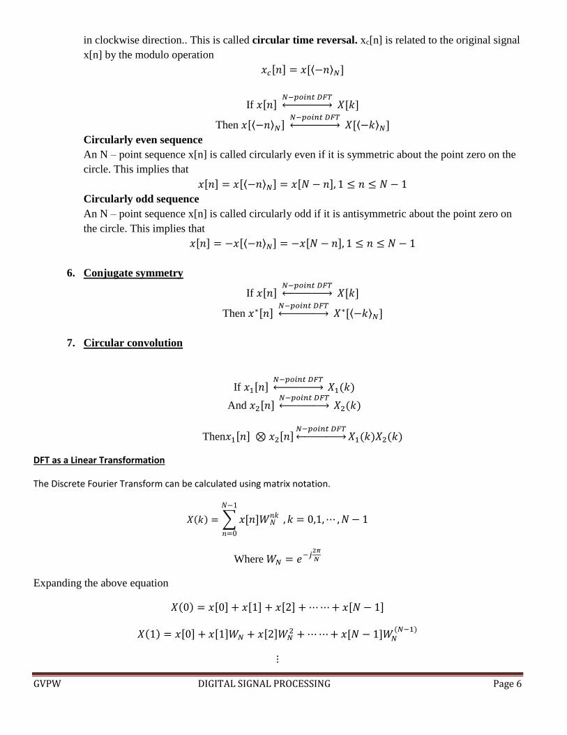
in clockwise direction.. This is called circular time reversal. xc[n] is related to the original signal

x[n] by the modulo operation

𝑥𝑐[𝑛] = 𝑥[⟨−𝑛⟩𝑁]


Then 𝑥[⟨−𝑛⟩𝑁] 𝑁−𝑝𝑜𝑖𝑛𝑡 𝐷𝐹𝑇↔ 𝑋[⟨−𝑘⟩𝑁]

Circularly even sequence

An N – point sequence x[n] is called circularly even if it is symmetric about the point zero on the

circle. This implies that

𝑥[𝑛] = 𝑥[⟨−𝑛⟩𝑁] = 𝑥[𝑁 − 𝑛], 1 ≤ 𝑛 ≤ 𝑁 − 1

Circularly odd sequence

An N – point sequence x[n] is called circularly odd if it is antisymmetric about the point zero on

the circle. This implies that

𝑥[𝑛] = −𝑥[⟨−𝑛⟩𝑁] = −𝑥[𝑁 − 𝑛], 1 ≤ 𝑛 ≤ 𝑁 − 1

6. Conjugate symmetry


Then 𝑥∗[𝑛] 𝑁−𝑝𝑜𝑖𝑛𝑡 𝐷𝐹𝑇↔ 𝑋∗[⟨−𝑘⟩𝑁]

7. Circular convolution

If 𝑥1[𝑛] 𝑁−𝑝𝑜𝑖𝑛𝑡 𝐷𝐹𝑇↔ 𝑋1(𝑘)

And 𝑥2[𝑛] 𝑁−𝑝𝑜𝑖𝑛𝑡 𝐷𝐹𝑇↔ 𝑋2(𝑘)

Then𝑥1[𝑛] ⊗ 𝑥2[𝑛]𝑁−𝑝𝑜𝑖𝑛𝑡 𝐷𝐹𝑇↔ 𝑋1(𝑘)𝑋2(𝑘)

DFT as a Linear Transformation

The Discrete Fourier Transform can be calculated using matrix notation.

𝑋(𝑘) = ∑ 𝑥[𝑛]𝑊𝑁𝑛𝑘

𝑁−1

𝑛=0

, 𝑘 = 0,1,⋯ ,𝑁 − 1

Where 𝑊𝑁 = 𝑒−𝑗2𝜋

𝑁

Expanding the above equation

𝑋(0) = 𝑥[0] + 𝑥[1] + 𝑥[2] + ⋯⋯+ 𝑥[𝑁 − 1]

𝑋(1) = 𝑥[0] + 𝑥[1]𝑊𝑁 + 𝑥[2]𝑊𝑁2 +⋯⋯+ 𝑥[𝑁 − 1]𝑊𝑁

(𝑁−1)

⋮


𝑋(𝑁 − 1) = 𝑥[0] + 𝑥[1]𝑊𝑁(𝑁−1) + 𝑥[2]𝑊𝑁

2(𝑁−1) +⋯⋯+ 𝑥[𝑁 − 1]𝑊𝑁(𝑁−1)(𝑁−1)

Expressing the above set of equations in matrix notation, we obtain

[ 𝑋(0)𝑋(1)𝑋(2)⋮

𝑋(𝑁 − 1)]

=

[ 1 1 1 ⋯ 1

1 𝑊𝑁 𝑊𝑁2 ⋯ 𝑊𝑁

(𝑁−1)

1 𝑊𝑁2 𝑊𝑁

4 ⋯ 𝑊𝑁2(𝑁−1)

⋮ ⋮ ⋮ ⋯ ⋮

1 𝑊𝑁(𝑁−1)

𝑊𝑁2(𝑁−1)

⋯ 𝑊𝑁(𝑁−1)(𝑁−1)

]

[ 𝑥[0]𝑥[1]𝑥[2]⋮

𝑥[𝑁 − 1]]

𝑜𝑟, �̅� = 𝑾𝑵̅̅ ̅̅ ̅ �̅� ………𝐸𝑞𝑛. 𝐴

Similarly, for the IDFT equation, 𝑥[𝑛] =1

𝑁∑ 𝑋(𝑘)𝑊𝑁

−𝑛𝑘𝑁−1𝑛=0 , 𝑛 = 0, 1,⋯ ,𝑁 − 1, the matrix notation would

be

�̅� =1

𝑁𝑾𝑵̅̅ ̅̅ ̅∗ �̅� ………𝐸𝑞𝑛 𝐵

But, from equation A,

�̅� = 𝑾𝑵̅̅ ̅̅ ̅−𝟏 �̅� …… . . 𝐸𝑞𝑛. 𝐶

From Equations B & C, we have

𝑾𝑵̅̅ ̅̅ ̅−𝟏 =

1

𝑁𝑾𝑵̅̅ ̅̅ ̅∗

Linear Convolution Using Circular Convolution

The output of an LTI system is the linear convolution of the input x[n] and the system’s impulse response

h[n]. the DFT is a practical approach for implementing linear system operations in the frequency domain.

But, the problem is, the DFT operations result in a circular convolution in time domain , and not the linear

convolution. i.e., 𝑋1(𝑘)𝑋2(𝑘)𝑁−𝑝𝑜𝑖𝑛𝑡 𝐼𝐷𝐹𝑇↔ 𝑥1[𝑛] ⊗ 𝑥2[𝑛]

Let x[n] be of length Nx and h[n] be of length Nh, and let Nx > Nh. then, the result of linear convolution is of

length N = Nx + Nh – 1 , whereas that of cicular convolution is of length N = max (Nx, Nh).

For circular convolution to yield the same result as the linear convolution, both the sequences must be zero –

padded so that both are of length Nx + Nh – 1. Let the padded sequences be xp[n] and hp[n]. then we compute

the N (= Nx + Nh – 1) point circular convolution of xp[n] and hp[n], resulting in a sequence equal to the linear

convolution x[n]*h[n].

i.e., 𝑋𝑝(𝑘)𝐻𝑝(𝑘)𝑁−𝑝𝑜𝑖𝑛𝑡 𝐼𝐷𝐹𝑇↔ 𝑥[𝑛] ∗ ℎ[𝑛]

Filtering of Long Data sequences using DFT

To filter signals like speech signals, etc., which are long data sequences, using DFT, it is required to compute

a large DFT. Moreover, the output samples are not available until all the input samples are produced , thus


introducing an unacceptably large amount of delay. To overcome this problem, the input sequence is divided

into smaller sections/blocks, and each block is processed via DFT and IDFT to produce a block of output

data. The output blocks are fitted together to yield the final output sequence. This procedure is called

sectioned / block convolution. There are two ways to do this: overlap – save method and overlap – add

method.

Overlap – save method

Let h[n] be the impulse response of length M, and x[n] be the input sequence of length much greater than M.

• x[n] is divided into sections xr[n], each of length N, so that each input section overlaps the preceding

section by M – 1 samples.

• The first M – 1 samples of the first section are set to zero.

• Then, the N – point circular convolution, yr[n] of each section xr[n] with h[n] is obtained.

• The first M – 1 samples of each output section must be discarded.

• The remaining N – M + 1 samples from each successive sections are concatenated to reconstruct the

final filtered output.

Overlap – add method

• x[n] is represented as a sum of finite – length segments of length N

𝑥[𝑛] = ∑𝑥𝑟𝑟

[𝑛 − 𝑟𝑁]

Where 𝑥𝑟[𝑛] = {𝑥[𝑛 + 𝑟𝑁], 0 ≤ 𝑛 ≤ 𝑁 − 1

0, 𝑒𝑙𝑠𝑒

• the final output of the filter is given by the linear convolution

𝑦[𝑛] = ℎ[𝑛] ∗ 𝑥[𝑛] = ℎ[𝑛] ∗ ∑𝑥𝑟𝑟

[𝑛 − 𝑟𝑁]

=∑𝑦𝑟𝑟

[𝑛 − 𝑟𝑁]

Where 𝑦𝑟[𝑛] = ℎ[𝑛] ∗ 𝑥𝑟[𝑛]

Since h[n] is of length M and 𝑥𝑟[𝑛] is of length N, the linear convolution result 𝑦𝑟[𝑛] is of length N +

M – 1, which can be obtained using N + M – 1 point DFTs.

• Since 𝑥𝑟[𝑛] is the section of x[n] starting at n = rN, so 𝑦𝑟[𝑛] also starts at n = rN. But, each 𝑦𝑟[𝑛] is

of length N + M – 1, whereas each 𝑥𝑟[𝑛] is of length N.

i.e.,

𝑦0[𝑛] = ℎ[𝑛] ∗ 𝑥0[𝑛], 0 ≤ 𝑛 ≤ 𝑁 +𝑀 − 2

𝑦1[𝑛] = ℎ[𝑛] ∗ 𝑥1[𝑛], 𝑁 ≤ 𝑛 ≤ 2𝑁 +𝑀 − 2

𝑦2[𝑛] = ℎ[𝑛] ∗ 𝑥2[𝑛], 2𝑁 ≤ 𝑛 ≤ 3𝑁 +𝑀 − 2, 𝑎𝑛𝑑 𝑠𝑜 𝑜𝑛


So, there is an overlap of M – 1 samples between every two consecutive sections. These overlapping

samples must be added to obtain final output.

Fast Fourier Transform (FFT)

Fast Fourier Transform is an efficient algorithm developed by Cooley & Tukey in 1965, used to compute the

DFT with reduced computations. Due to the efficiency of FFT, it is used for spectrum analysis, convolutions,

correlations and linear filtering.

FFT reduces the problem of calculating an N – point DFT to that of calculating many smaller – sized DFTs.

The properties of the twiddle factor WN used in this algorithm are:

1. 𝑊𝑁𝑘+

𝑁

2 = 𝑒−𝑗2𝜋𝑘

𝑁 𝑒−𝑗𝜋 = − 𝑊𝑁𝑘 (Symmetry Property)

2. 𝑊𝑁𝑘+𝑁 = 𝑒−

𝑗2𝜋𝑘

𝑁 𝑒−𝑗2𝜋 = 𝑊𝑁𝑘 (periodicity property)

3. 𝑊𝑁𝑚 = 𝑒−

𝑗2𝜋𝑚

𝑁 = 𝑒−𝑗2𝜋𝑁𝑚⁄ = 𝑊𝑁

𝑚⁄

The Decimation – In – Time (DIT) and Decimation – In – Frequency (DIF) FFT algorithms use the “divide –

and – conquer” approach. This is possible if the length of the sequence N is chosen as N = rm. here, r is called

the radix of the FFT algorithm. The most practically implemented choice for r = 2 leads to radix – 2 FFT

algorithms. So, with N = 2m, the efficient computation is achieved by breaking the N – point DFT into two 𝑁

2

- point DFTs, then breaking each 𝑁

2 - point DFT into two

𝑁

4 - point DFTs and continuing this process until 2 –

point DFTs are obtained. For N=8, the Decimation – In – Time algorithm decomposition would be

Decimation – In – Time (DIT) FFT algorithm


In this algorithm, the time – domain sequence x[n] is decimated into two 𝑁

2 – point sequences, one composed

of even – indexed values of x[n], and other composed of odd – indexed values of x[n].i.e.,

𝑔[𝑛] = 𝑥[2𝑛]……… . 𝑒𝑞𝑛. 1

𝑎𝑛𝑑, ℎ[𝑛] = 𝑥[2𝑛 + 1]……… . 𝑒𝑞𝑛. 2

The N – point DFT of x[n] is given by


𝑁−1

𝑛=0

, 𝑘 = 0,1,⋯ ,𝑁 − 1

This can be rewritten as


𝑁−1

𝑛=0,𝑒𝑣𝑒𝑛

+ ∑ 𝑥[𝑛]𝑊𝑁𝑛𝑘

𝑁−1

𝑛=0,𝑜𝑑𝑑

= ∑ 𝑥[2𝑛]𝑊𝑁2𝑛𝑘

𝑁2−1

𝑛=0

+ ∑ 𝑥[2𝑛 + 1]𝑊𝑁(2𝑛+1)𝑘

𝑁2−1

𝑛=0

= ∑ 𝑥[2𝑛]𝑊𝑁2𝑛𝑘

𝑁2−1

𝑛=0

+ 𝑊𝑁𝑘∑𝑥[2𝑛 + 1]𝑊𝑁

2𝑛𝑘

𝑁2−1

𝑛=0

Using the third property of the twiddle factor, WN, the above equation can be rewritten as

= ∑ 𝑥[2𝑛]𝑊𝑁2⁄

𝑛𝑘

𝑁2−1

𝑛=0

+ 𝑊𝑁𝑘∑𝑥[2𝑛 + 1]𝑊𝑁

2⁄𝑛𝑘

𝑁2−1

𝑛=0

Using equations 1 & 2 in the above equation, we obtain

𝑋(𝑘) = ∑ 𝑔[𝑛]𝑊𝑁2⁄

𝑛𝑘

𝑁2−1

𝑛=0

+ 𝑊𝑁𝑘∑ℎ[𝑛]𝑊𝑁

2⁄𝑛𝑘

𝑁2−1

𝑛=0

𝑜𝑟, 𝑋(𝑘) = 𝐺(𝑘) +𝑊𝑁𝑘𝐻(𝑘)……𝑒𝑞𝑛. 3

Where G(k) and H(k) are the N/2 – point DFTs of g[n] and h[n] respectively. So, G(k) and H(k) are periodic

with period N/2 .i.e.,

𝐺 (𝑘 +𝑁

2) = 𝐺(𝑘)……𝑒𝑞𝑛. 4

𝑎𝑛𝑑,𝐻 (𝑘 +𝑁

2) = 𝐻(𝑘)……𝑒𝑞𝑛. 5


And using the symmetry property of the twiddle factor, WN, and equations4 & 5

𝑋(𝑘 + 𝑁/2) = 𝐺(𝑘) −𝑊𝑁𝑘𝐻(𝑘)……𝑒𝑞𝑛. 6

Equations 3 and 6 result in the following butterfly diagram

For example, for N = 8, the DFT points in terms of G and H are

𝑋(0) = 𝐺(0) +𝑊𝑁0𝐻(0)

𝑋(1) = 𝐺(1) +𝑊𝑁1𝐻(1)

𝑋(2) = 𝐺(2) +𝑊𝑁2𝐻(2)

𝑋(3) = 𝐺(3) +𝑊𝑁3𝐻(3)

For the remaining 4 points X(4) to X(7), we use equations 4, 5, 6 and 7 to get

𝑋(4) = 𝐺(0) −𝑊𝑁0𝐻(0)

𝑋(5) = 𝐺(1) −𝑊𝑁1𝐻(1)

𝑋(6) = 𝐺(2) −𝑊𝑁2𝐻(2)

𝑋(7) = 𝐺(3) −𝑊𝑁3𝐻(3)

The butterfly diagram for the above set of equations is


The above process is repeated for calculating the N/2 point DFTs of g[n] and h[n], and this is continued till

we get two point DFTs. Once we reach a two – point sequence, say p[n]={p[0], p[1]}, its 2 – point DFT

would be

𝑃(𝑘) = ∑ 𝑝[𝑛]𝑊2𝑛𝑘

1

𝑛=0

, 𝑘 = 0,1

𝑜𝑟, 𝑃(𝑘) = 𝑝[0] + 𝑝[1]𝑊2𝑘, , 𝑘 = 0,1

⇒ 𝑃(0) = 𝑝[0] + 𝑝[1]

𝑎𝑛𝑑 𝑃(1) = 𝑝[0] +𝑊2𝑝[1] = 𝑝[0] − 𝑝[1]

The overall butterfly diagram for DIT FFT algorithm for N =8 is


Due to repeated decimations, the input sequence is scrambled, and the order of the final input sequence is

obtained as follows

Input sequence Index Binary form of

index

Bit reversed

form of index

Decimal

representation

Final input

sequence order

x[0] 0 000 000 0 x[0]

x[1] 1 001 100 4 x[4]

x[2] 2 010 010 2 x[2]

x[3] 3 011 110 6 x[6]

x[4] 4 100 001 1 x[1]

x[5] 5 101 101 5 x[5]

x[6] 6 110 011 3 x[3]

x[7] 7 111 111 7 x[7]

Decimation – In – Frequency (DIF) FFT algorithm

In this algorithm, we decimate the DFT sequence X(k) into smaller and smaller subsequences (Instead of the

time – domain sequence x[n]).


𝑁−1

𝑛=0

=∑ 𝑥[𝑛]𝑊𝑁𝑛𝑘

𝑁2−1

𝑛=0

+∑ 𝑥[𝑛]𝑊𝑁𝑛𝑘

𝑁−1

𝑛=𝑁2

= ∑ 𝑥[𝑛]𝑊𝑁𝑛𝑘

𝑁2−1

𝑛=0

+∑ 𝑥[𝑛 +𝑁

2]𝑊𝑁

𝑛𝑘

𝑁2−1

𝑛=0

𝑊𝑁

𝑁2𝑘

𝑏𝑢𝑡,𝑊𝑁

𝑁2𝑘= (−1)𝑘


𝑋(𝑘) = ∑ {𝑥[𝑛] + (−1)𝑘𝑥 [𝑛 +𝑁

2]}𝑊𝑁

𝑛𝑘

𝑁2−1

𝑛=0

, 𝑘 = 0,1, … ,𝑁 − 1

Now, decimating X(k) into even and odd – indexed samples,

𝑋(2𝑘) = ∑ {𝑥[𝑛] + 𝑥 [𝑛 +𝑁

2]}𝑊𝑁

2

𝑛𝑘

𝑁2−1

𝑛=0

, 𝑘 = 0,1, … ,𝑁

2− 1……𝑒𝑞𝑛. 1

𝑋(2𝑘 + 1) = ∑ {𝑥[𝑛] − 𝑥 [𝑛 +𝑁

2]}𝑊𝑁

𝑛 𝑊𝑁2

𝑛𝑘

𝑁2−1

𝑛=0

, 𝑘 = 0,1, … ,𝑁

2− 1……𝑒𝑞𝑛. 2

𝑙𝑒𝑡 𝑔[𝑛] = 𝑥[𝑛] + 𝑥 [𝑛 +𝑁

2] , 0 ≤ 𝑛 ≤

𝑁

2− 1……𝑒𝑞𝑛. 3

𝑎𝑛𝑑, ℎ[𝑛] = {𝑥[𝑛] − 𝑥 [𝑛 +𝑁

2]}𝑊𝑁

𝑛, 0 ≤ 𝑛 ≤𝑁

2− 1……𝑒𝑞𝑛. 4

Substituting equations 3 & 4 in equations 1 & 2 respectively

𝐺(𝑘) = 𝑋(2𝑘), 0 ≤ 𝑘 ≤𝑁

2− 1

𝑎𝑛𝑑, 𝐻(𝑘) = 𝑋(2𝑘 + 1) 0 ≤ 𝑘 ≤𝑁

2− 1

For example, for N=8, using equations 3 & 4, we get

𝑔[0] = 𝑥[0] + 𝑥[4]

𝑔[1] = 𝑥[1] + 𝑥[5]

𝑔[2] = 𝑥[2] + 𝑥[6]

𝑔[3] = 𝑥[3] + 𝑥[7]

ℎ[0] = {𝑥[0] − 𝑥[4]}𝑊80

ℎ[1] = {𝑥[1] − 𝑥[5]}𝑊81

ℎ[2] = {𝑥[2] − 𝑥[6]}𝑊82

ℎ[3] = {𝑥[3] − 𝑥[7]}𝑊83


the butterfly diagram for the above set of equations is as follows

The above process of decimation is repeated for G(k) and H(k), until we reach a 2 – point sequence. The 2 –

point DFT is calculated as in the previous section. The final butterfly diagram for Decimation – In –

Frequency FFT algorithm for N = 8 is as follows


In this algorithm, the output X(k) is in bit –reversed order.

Efficiency of FFT algorithm

A direct computation of DFT requires a large number of multiplications and additions. An N – point DFT is

given by


𝑁−1

𝑛=0

, 𝑘 = 0,1,⋯ ,𝑁 − 1

In the above equation, each DFT point computation involves N complex multiplications and (N – 1) complex

additions. So, the N – point DFT calculations involve N2 complex multiplications and N(N – 1) complex

additions. This means approximately 106 complex multiplications and additions for a 1024 – point

sequence.

On the other hand, in an FFT algorithm, a basic butterfly in DIT – FFT algorithm is represented as

And for DIF – FFT algorithm, it is represented as

• Number of stages in a butterfly diagram =log2𝑁

• Number of butterflies in each stage=N/2

• Number of complex multiplications in each butterfly=1

• Number of complex additions in each butterfly=2.


From the above, for an N – point FFT algorithm,

• Total number of complex multiplications =𝑁

2log2𝑁

• Total number of complex additions = 𝑁 log2𝑁

For a 1024 – point sequence, this means approximately 5120 complex multiplications and 10240

complex additions. i.e., approximately 100 times less additions and 200 times less multiplications than

direct computation of DFT.

As the number of input samples increase, the savings in the number of computations also increase.

In – Place computations

Another advantage of FFT algorithm is In – Place computations. As shown in the previous diagram of a basic

butterfly, any butterfly calculation involves 2 complex inputs a and b, and 2 complex outputs A and B. once,

these two outputs are calculated, the inputs of the butterfly are not used in any other calculation. So, A and B

can be stored in the same memory locations as a and b. this is called In – Place computation.

Inverse FFT Algorithm

Let X(k) be the N – point DFT of a length – N sequence x[n]. The inverse DFT is given by

𝑥[𝑛] =1

𝑁∑𝑋(𝑘)𝑊𝑁

−𝑛𝑘

𝑁−1

𝑛=0

, 𝑛 = 0, 1,⋯ , 𝑁 − 1

𝑜𝑟, 𝑥[𝑛] =1

𝑁∑ 𝑋(𝑘)(𝑊𝑁

𝑛𝑘)∗𝑁−1

𝑛=0

, 𝑛 = 0, 1,⋯ ,𝑁 − 1

An FFT algorithm can be used to compute the inverse DFT by replacing x[n] by X(k), taking the negative

powers of WN, and dividing the output by N. Hence, in order to compute the inverse DFT from an FFT

algorithm, following steps can be followed

• Take X(k) as the input sequence and x[n] as the output sequence

• Compute FFT by replacing the twiddle factors WN by 𝑊𝑁−1

• Divide the output sequence by N

So, the DIT – FFT algorithm becomes DIF Inverse FFT algorithm and vice – versa.

For example the DIT – Inverse FFT butterfly diagram for N =8 would be as follows


Date post:	19-Apr-2020
Category:	Documents
Upload:	others
View:	8 times
Download:	0 times

LECTURE NOTES ON DIGITAL SIGNAL PROCESSING...

Documents