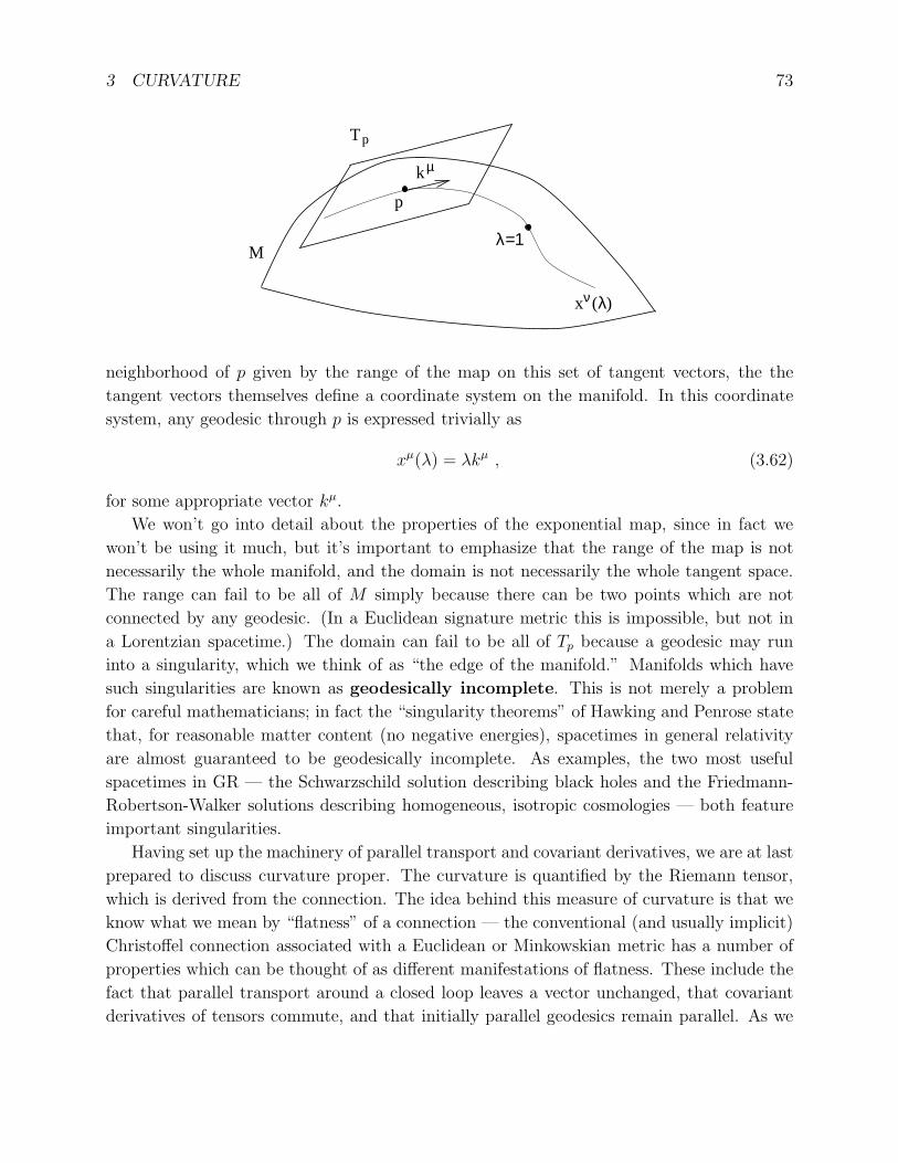
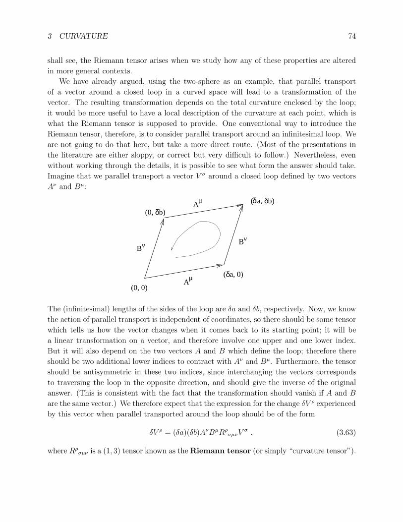
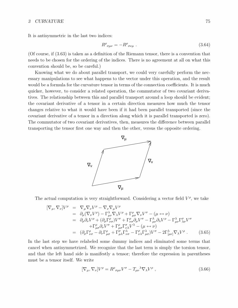
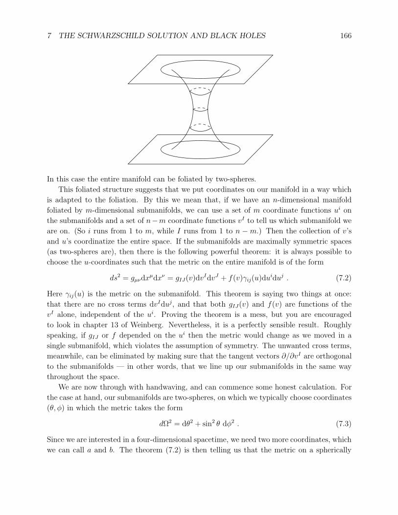
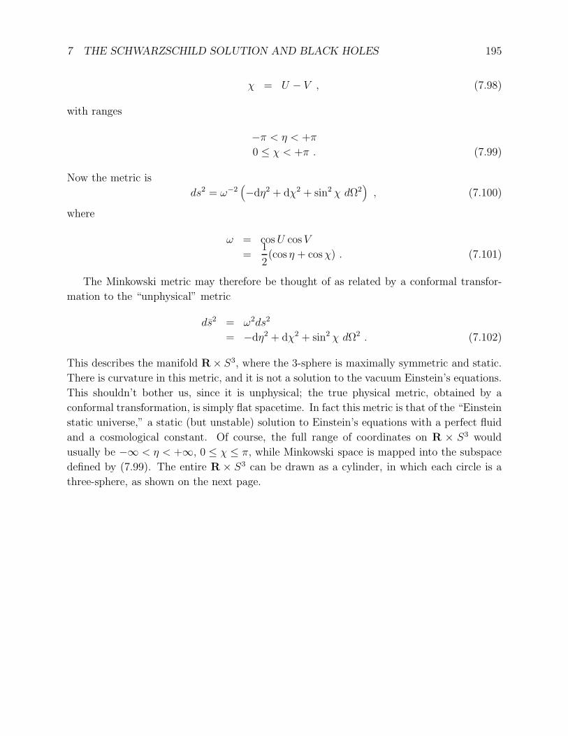
arXiv:gr-qc/9712019v1 3 Dec 1997 Lecture Notes on General Relativity Sean M. Carroll Institute for Theoretical Physics University of California Santa Barbara, CA 93106 [email protected]December 1997 Abstract These notes represent approximately one semester’s worth of lectures on intro- ductory general relativity for beginning graduate students in physics. Topics include manifolds, Riemannian geometry, Einstein’s equations, and three applications: grav- itational radiation, black holes, and cosmology. Individual chapters, and potentially updated versions, can be found at http://itp.ucsb.edu/~carroll/notes/. NSF-ITP/97-147 gr-qc/9712019
It is frequently useful to consider contractions of the Riemann tensor. Even without the
metric, we can form a contraction known as the Ricci tensor:
Rµν = Rλµλν . (3.90)
Notice that, for the curvature tensor formed from an arbitrary (not necessarily Christoffel)
connection, there are a number of independent contractions to take. Our primary concern is
with the Christoffel connection, for which (3.90) is the only independent contraction (modulo
conventions for the sign, which of course change from place to place). The Ricci tensor
associated with the Christoffel connection is symmetric,
Rµν = Rνµ , (3.91)
as a consequence of the various symmetries of the Riemann tensor. Using the metric, we can
take a further contraction to form the Ricci scalar:
R = Rµµ = gµνRµν . (3.92)
An especially useful form of the Bianchi identity comes from contracting twice on (3.87):
0 = gνσgµλ(∇λRρσµν + ∇ρRσλµν + ∇σRλρµν)
= ∇µRρµ −∇ρR + ∇νRρν , (3.93)
or
∇µRρµ =1
2∇ρR . (3.94)
(Notice that, unlike the partial derivative, it makes sense to raise an index on the covariant
derivative, due to metric compatibility.) If we define the Einstein tensor as
Gµν = Rµν −1
2Rgµν , (3.95)
then we see that the twice-contracted Bianchi identity (3.94) is equivalent to
∇µGµν = 0 . (3.96)
3 CURVATURE 82
The Einstein tensor, which is symmetric due to the symmetry of the Ricci tensor and the
metric, will be of great importance in general relativity.
The Ricci tensor and the Ricci scalar contain information about “traces” of the Riemann
tensor. It is sometimes useful to consider separately those pieces of the Riemann tensor
which the Ricci tensor doesn’t tell us about. We therefore invent the Weyl tensor, which is
basically the Riemann tensor with all of its contractions removed. It is given in n dimensions
by
Cρσµν = Rρσµν −2
(n− 2)
(gρ[µRν]σ − gσ[µRν]ρ
)+
2
(n− 1)(n− 2)Rgρ[µgν]σ . (3.97)
This messy formula is designed so that all possible contractions of Cρσµν vanish, while it
retains the symmetries of the Riemann tensor:
Cρσµν = C[ρσ][µν] ,
Cρσµν = Cµνρσ ,
Cρ[σµν] = 0 . (3.98)
The Weyl tensor is only defined in three or more dimensions, and in three dimensions it
vanishes identically. For n ≥ 4 it satisfies a version of the Bianchi identity,
∇ρCρσµν = −2(n− 3)
(n− 2)
(∇[µRν]σ +
1
2(n− 1)gσ[ν∇µ]R
). (3.99)
One of the most important properties of the Weyl tensor is that it is invariant under confor-
mal transformations. This means that if you compute Cρσµν for some metric gµν , and then
compute it again for a metric given by Ω2(x)gµν , where Ω(x) is an arbitrary nonvanishing
function of spacetime, you get the same answer. For this reason it is often known as the
“conformal tensor.”
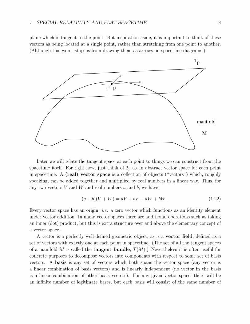
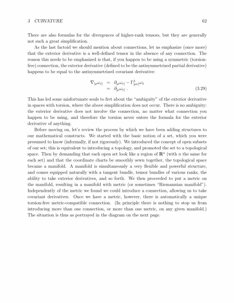
After this large amount of formalism, it might be time to step back and think about what
curvature means for some simple examples. First notice that, according to (3.85), in 1, 2, 3
and 4 dimensions there are 0, 1, 6 and 20 components of the curvature tensor, respectively.
(Everything we say about the curvature in these examples refers to the curvature associated
with the Christoffel connection, and therefore the metric.) This means that one-dimensional
manifolds (such as S1) are never curved; the intuition you have that tells you that a circle is
curved comes from thinking of it embedded in a certain flat two-dimensional plane. (There is
something called “extrinsic curvature,” which characterizes the way something is embedded
in a higher dimensional space. Our notion of curvature is “intrinsic,” and has nothing to do
with such embeddings.)
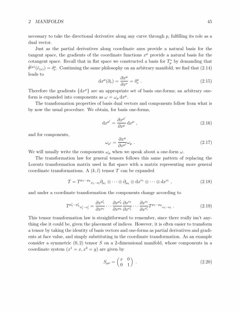
The distinction between intrinsic and extrinsic curvature is also important in two dimen-
sions, where the curvature has one independent component. (In fact, all of the information
3 CURVATURE 83
identify
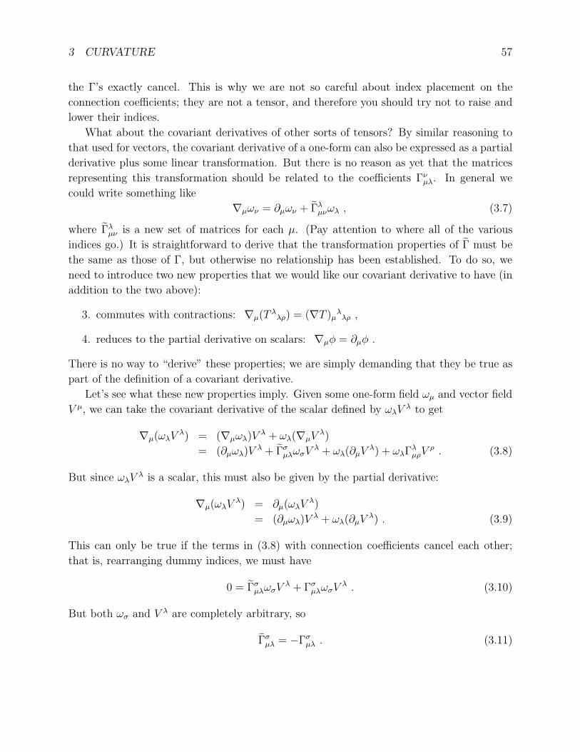
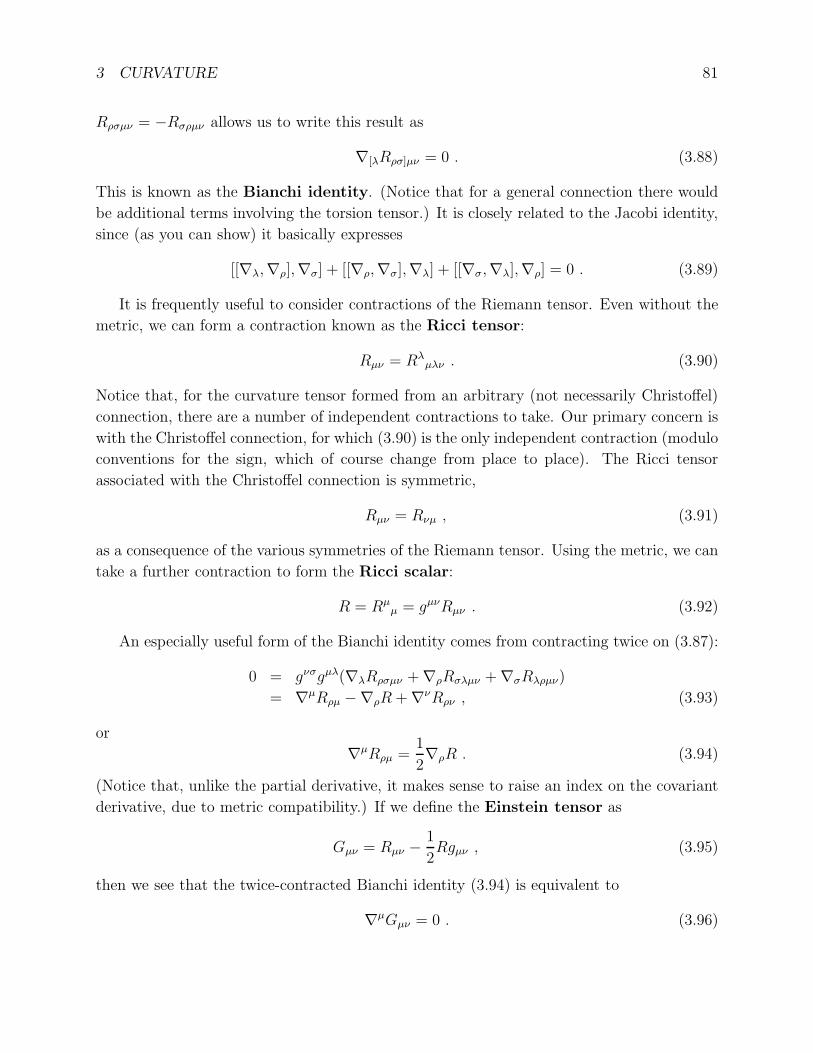
about the curvature is contained in the single component of the Ricci scalar.) Consider a
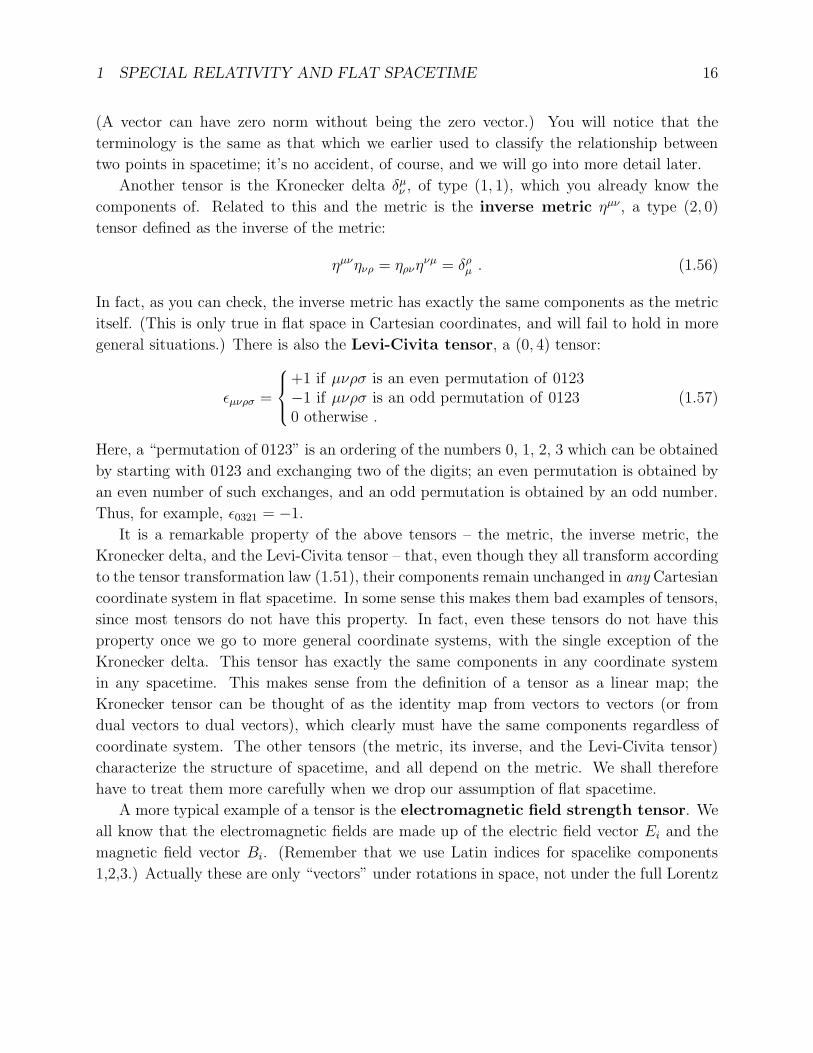
cylinder, R × S1. Although this looks curved from our point of view, it should be clear
that we can put a metric on the cylinder whose components are constant in an appropriate
coordinate system — simply unroll it and use the induced metric from the plane. In this
metric, the cylinder is flat. (There is also nothing to stop us from introducing a different
metric in which the cylinder is not flat, but the point we are trying to emphasize is that it
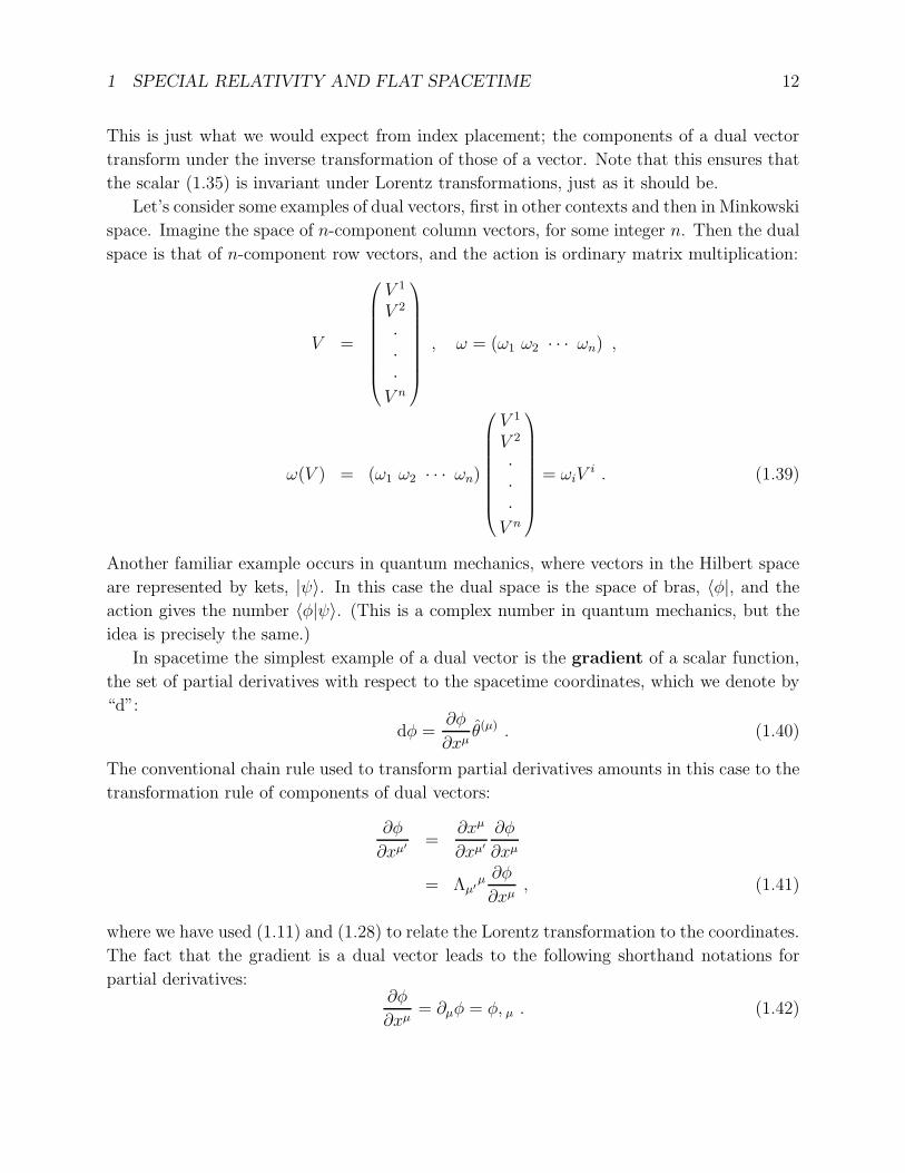
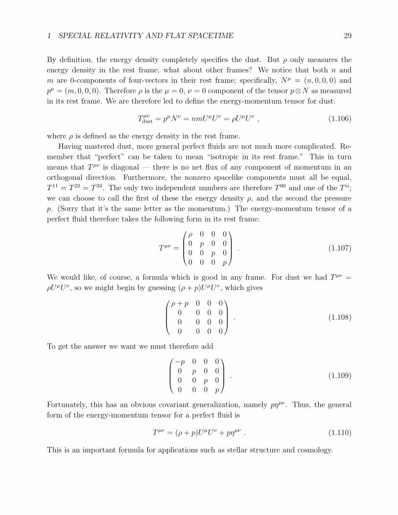
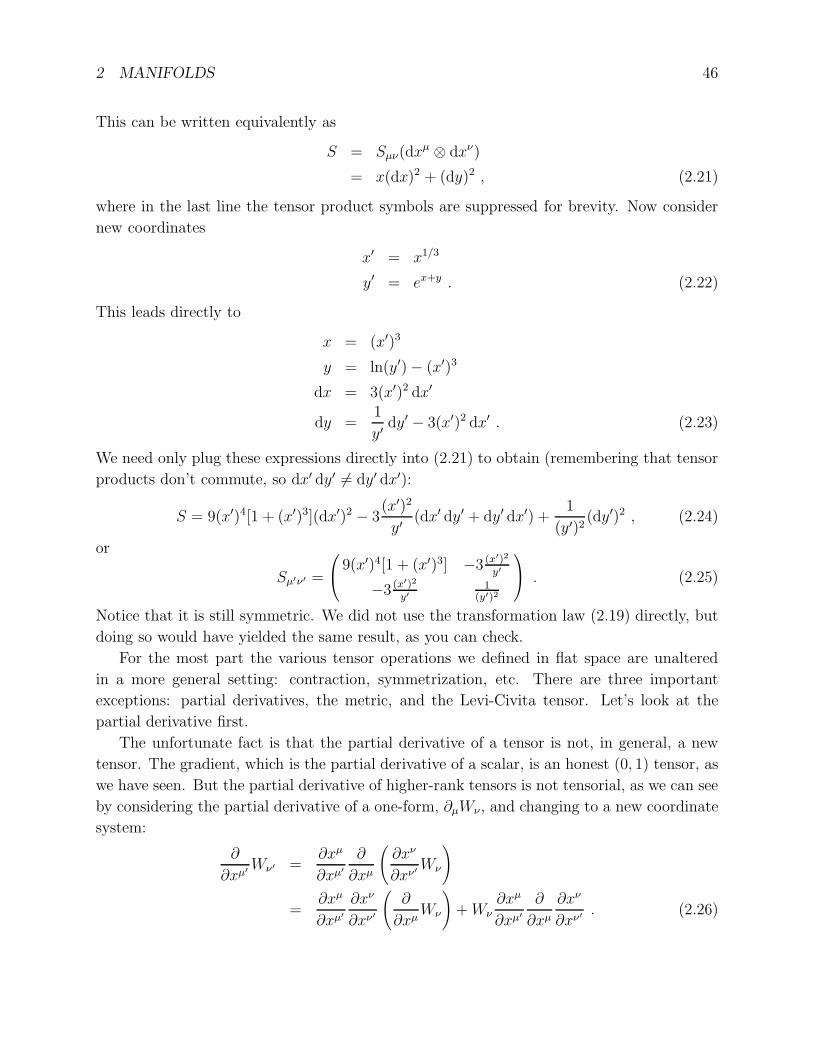
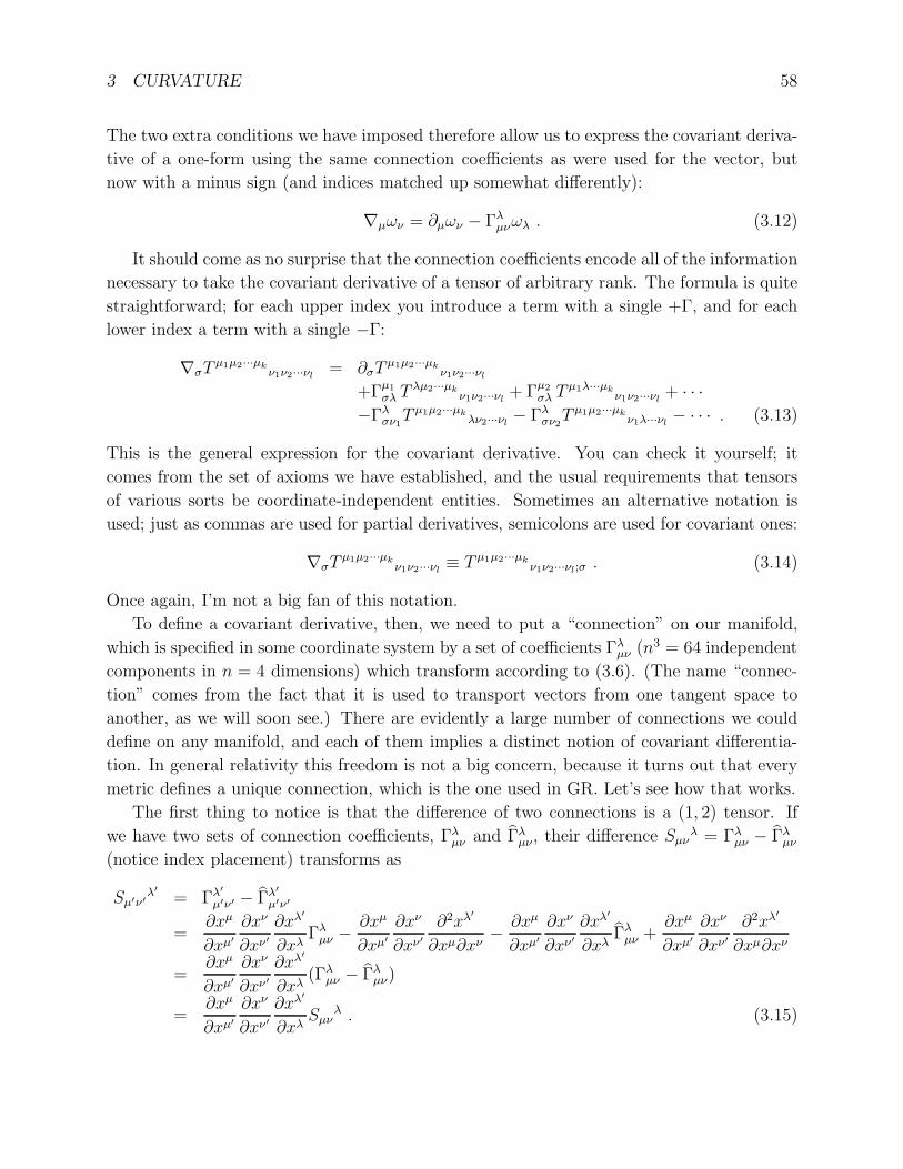
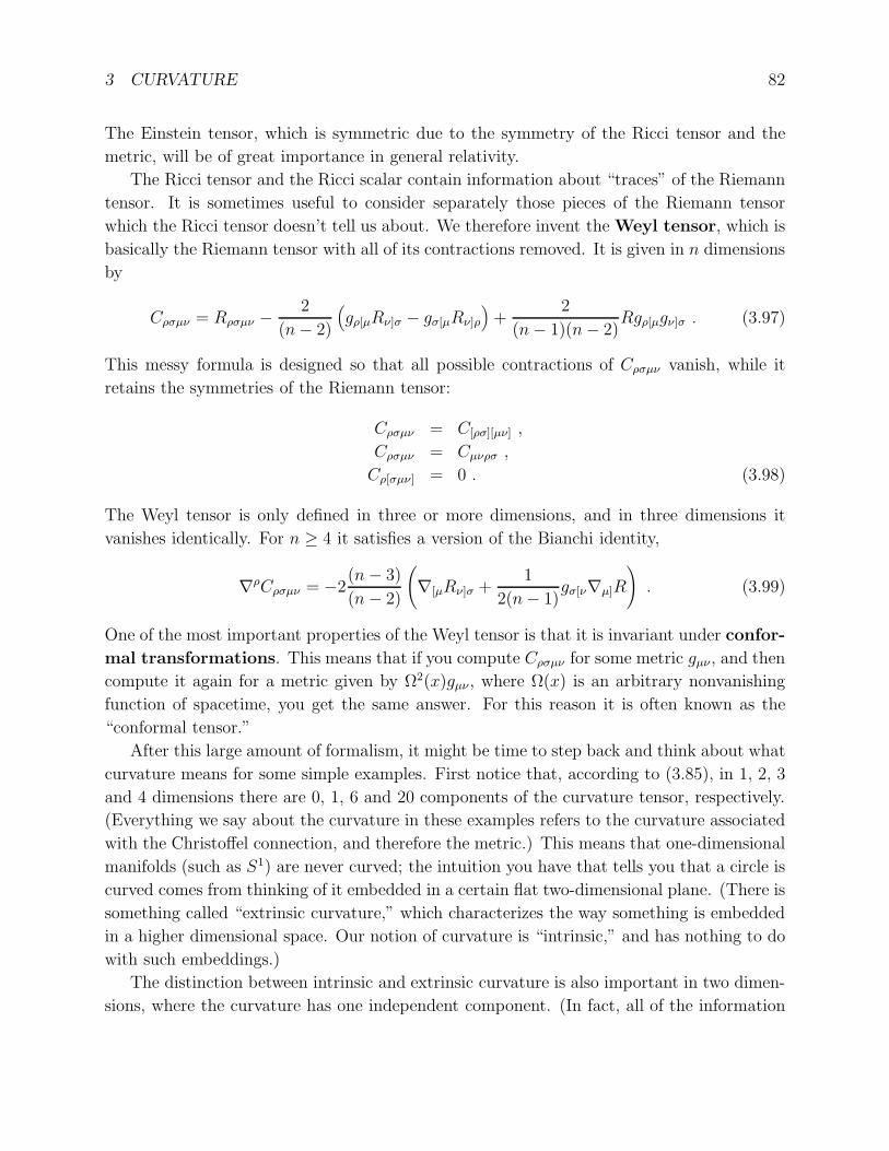
can be made flat in some metric.) The same story holds for the torus:
identify
We can think of the torus as a square region of the plane with opposite sides identified (in
other words, S1 × S1), from which it is clear that it can have a flat metric even though it
looks curved from the embedded point of view.
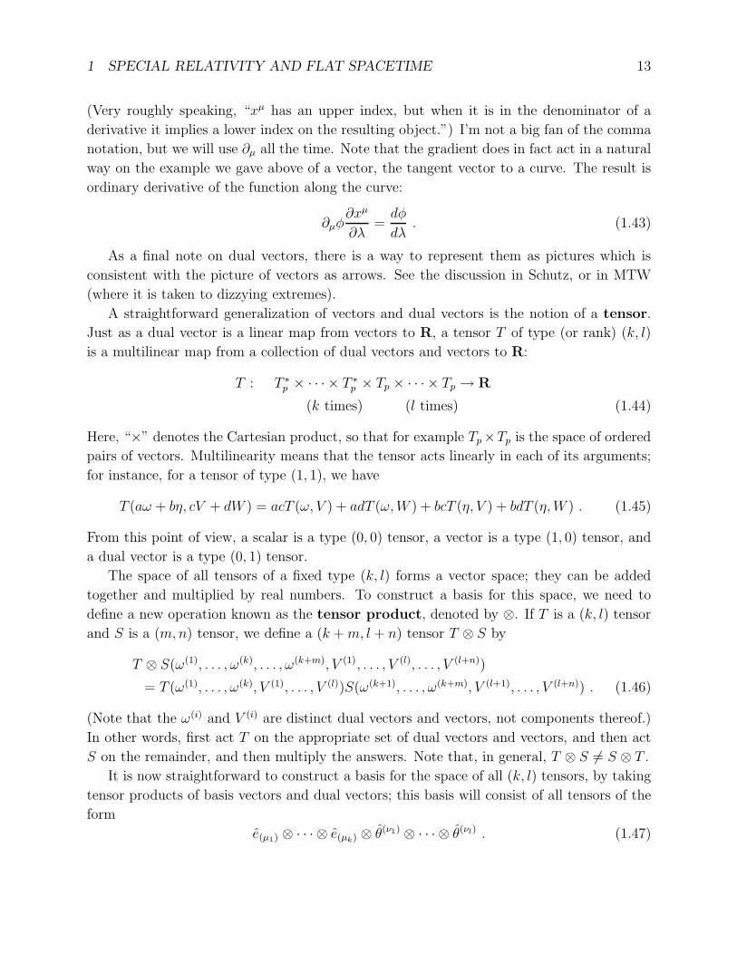
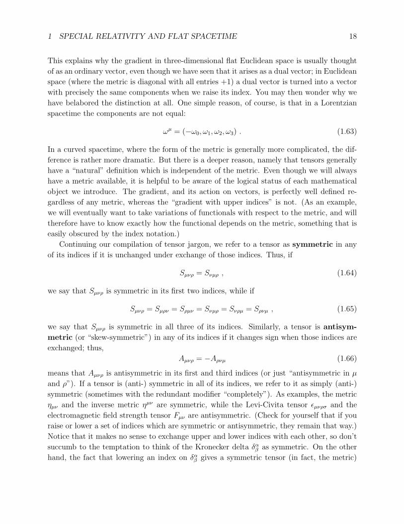
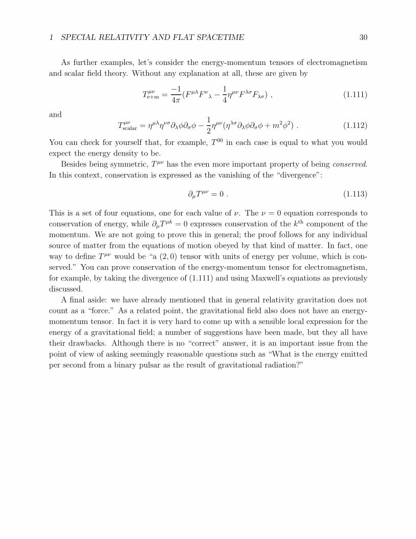
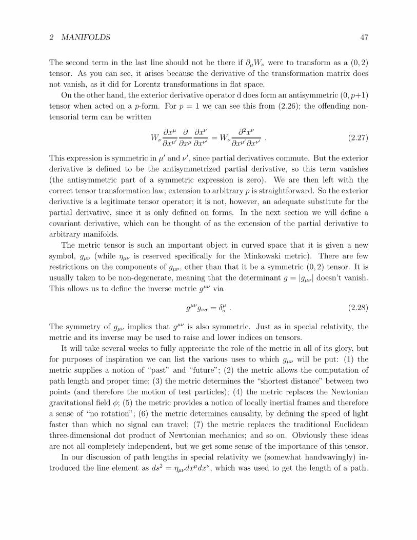
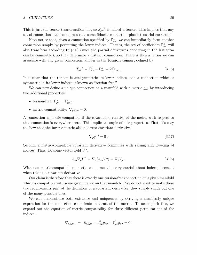
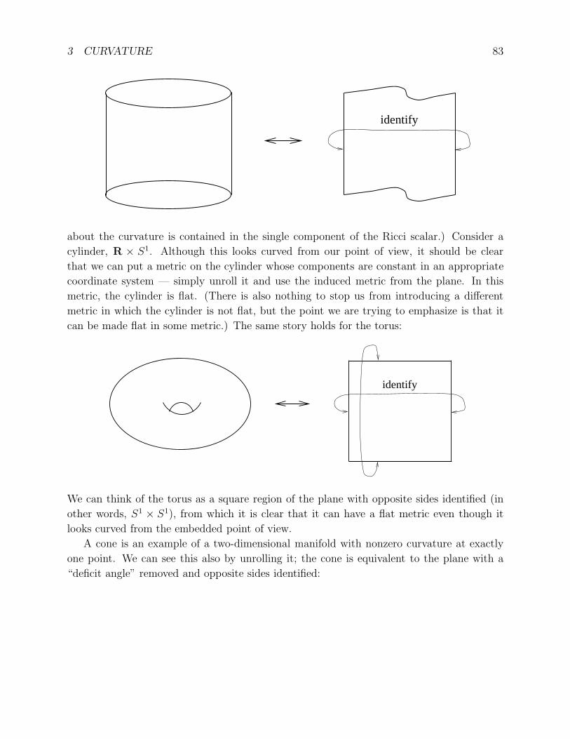
A cone is an example of a two-dimensional manifold with nonzero curvature at exactly
one point. We can see this also by unrolling it; the cone is equivalent to the plane with a
“deficit angle” removed and opposite sides identified:
3 CURVATURE 84
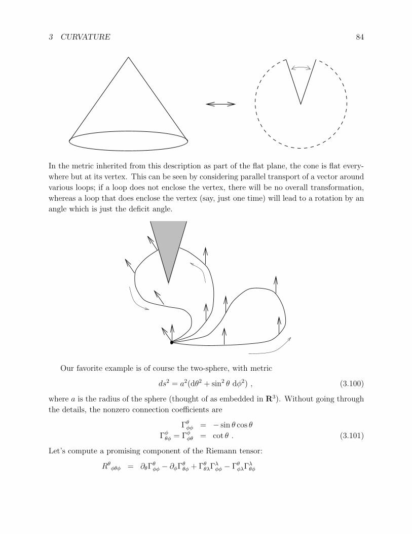
In the metric inherited from this description as part of the flat plane, the cone is flat every-
where but at its vertex. This can be seen by considering parallel transport of a vector around
various loops; if a loop does not enclose the vertex, there will be no overall transformation,
whereas a loop that does enclose the vertex (say, just one time) will lead to a rotation by an
angle which is just the deficit angle.
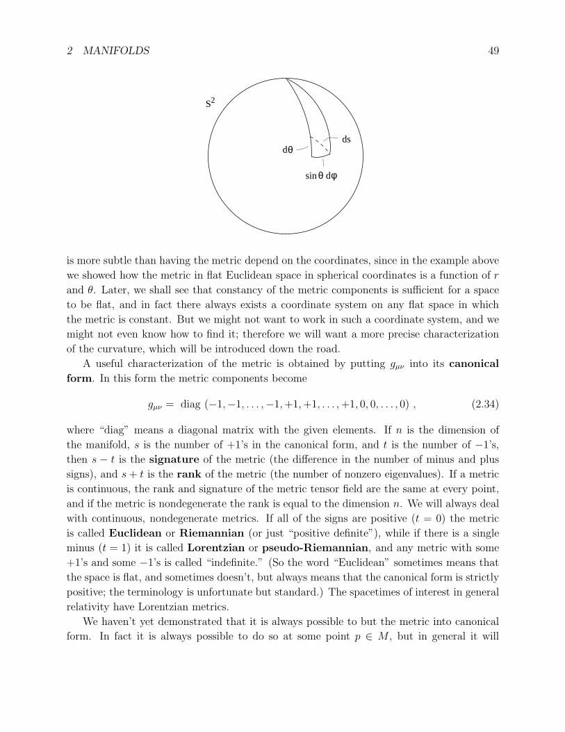
Our favorite example is of course the two-sphere, with metric
ds2 = a2(dθ2 + sin2 θ dφ2) , (3.100)
where a is the radius of the sphere (thought of as embedded in R3). Without going through
the details, the nonzero connection coefficients are
Γθφφ = − sin θ cos θ
Γφθφ = Γφ
φθ = cot θ . (3.101)
Let’s compute a promising component of the Riemann tensor:
Rθφθφ = ∂θΓ
θφφ − ∂φΓθ
θφ + ΓθθλΓ
λφφ − Γθ
φλΓλθφ
3 CURVATURE 85
= (sin2 θ − cos2 θ) − (0) + (0) − (− sin θ cos θ)(cot θ)
= sin2 θ . (3.102)
(The notation is obviously imperfect, since the Greek letter λ is a dummy index which is
summed over, while the Greek letters θ and φ represent specific coordinates.) Lowering an
index, we have
Rθφθφ = gθλRλ
φθφ
= gθθRθφθφ
= a2 sin2 θ . (3.103)
It is easy to check that all of the components of the Riemann tensor either vanish or are
related to this one by symmetry. We can go on to compute the Ricci tensor via Rµν =
gαβRαµβν . We obtain
Rθθ = gφφRφθφθ = 1
Rθφ = Rφθ = 0
Rφφ = gθθRθφθφ = sin2 θ . (3.104)
The Ricci scalar is similarly straightforward:
R = gθθRθθ + gφφRφφ =2
a2. (3.105)
Therefore the Ricci scalar, which for a two-dimensional manifold completely characterizes
the curvature, is a constant over this two-sphere. This is a reflection of the fact that the
manifold is “maximally symmetric,” a concept we will define more precisely later (although it
means what you think it should). In any number of dimensions the curvature of a maximally
symmetric space satisfies (for some constant a)
Rρσµν = a−2(gρµgσν − gρνgσµ) , (3.106)
which you may check is satisfied by this example.
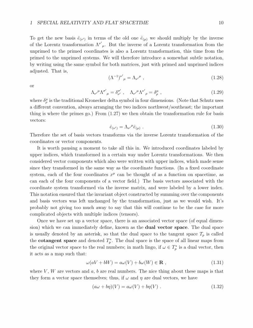
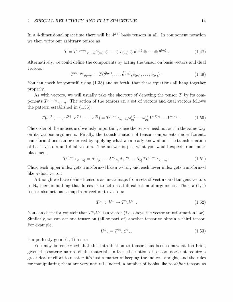
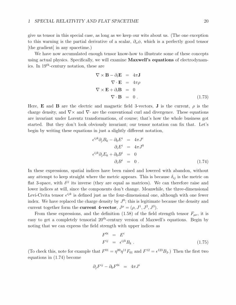
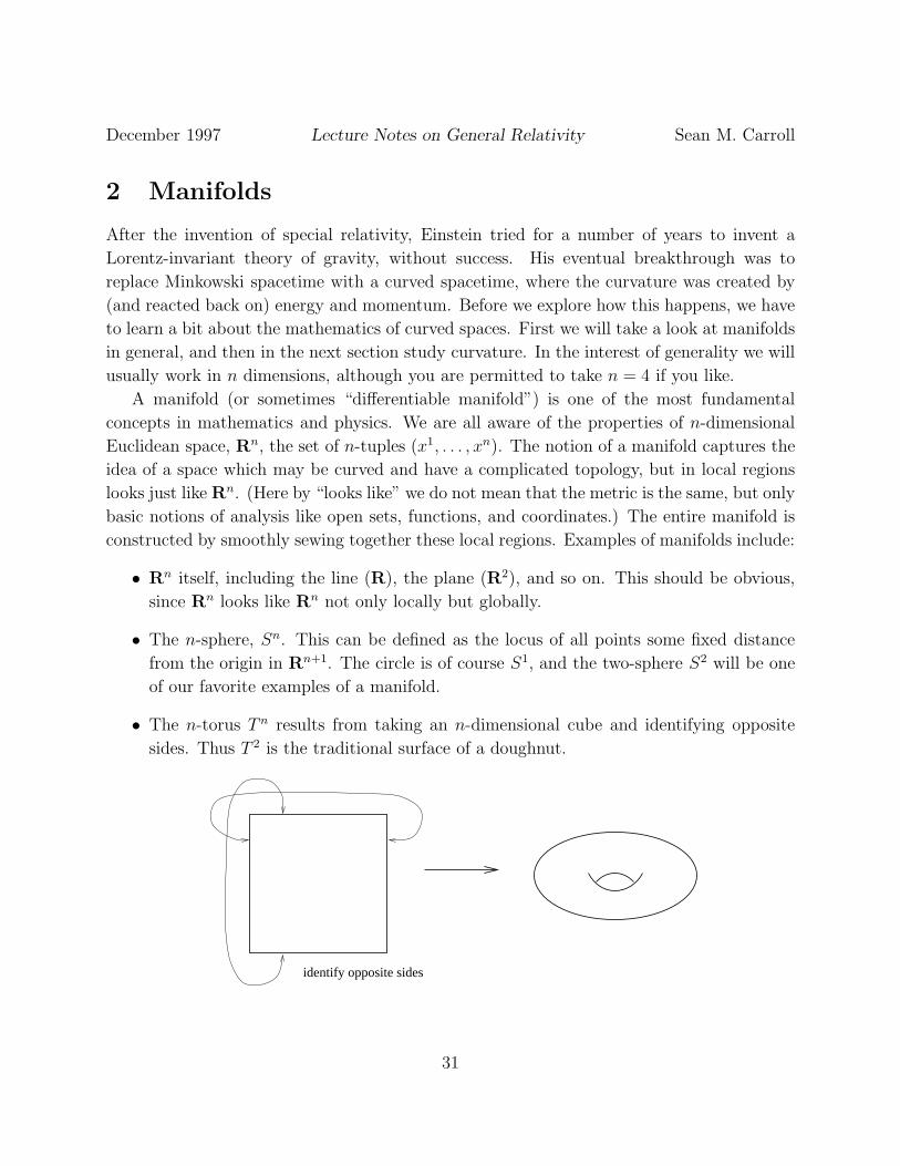
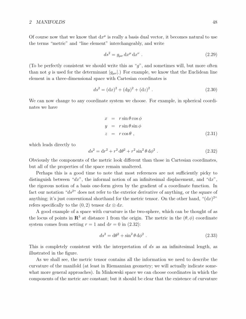
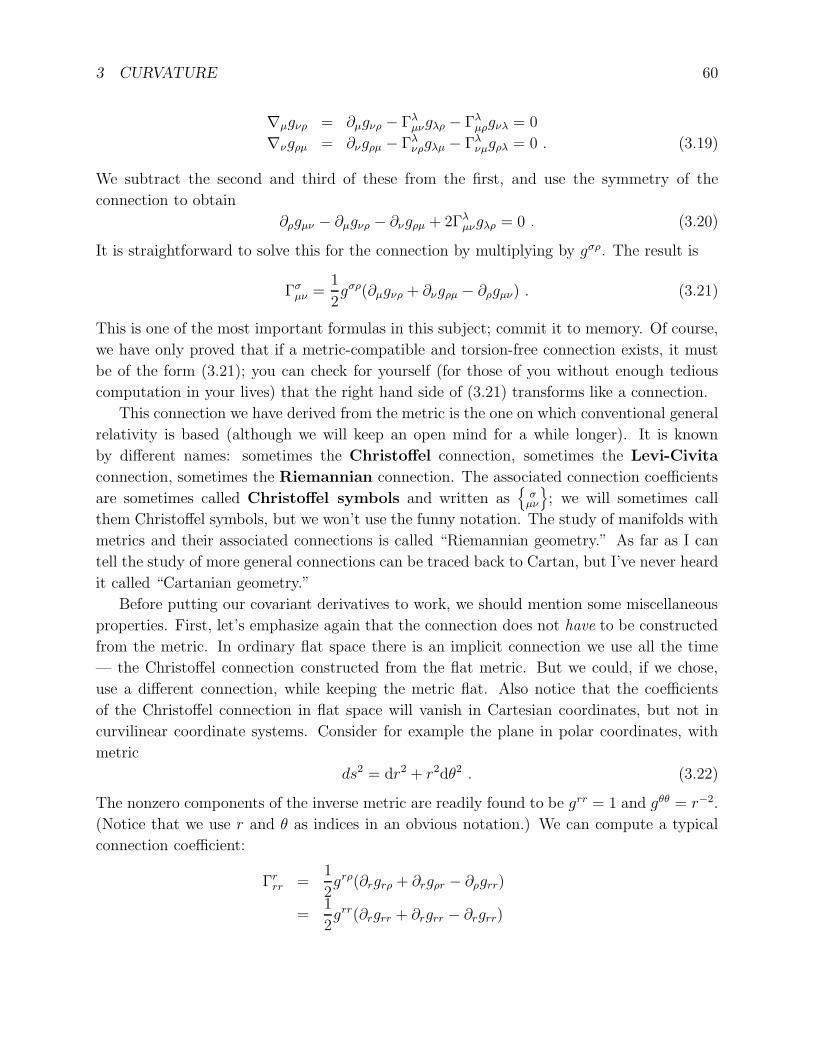
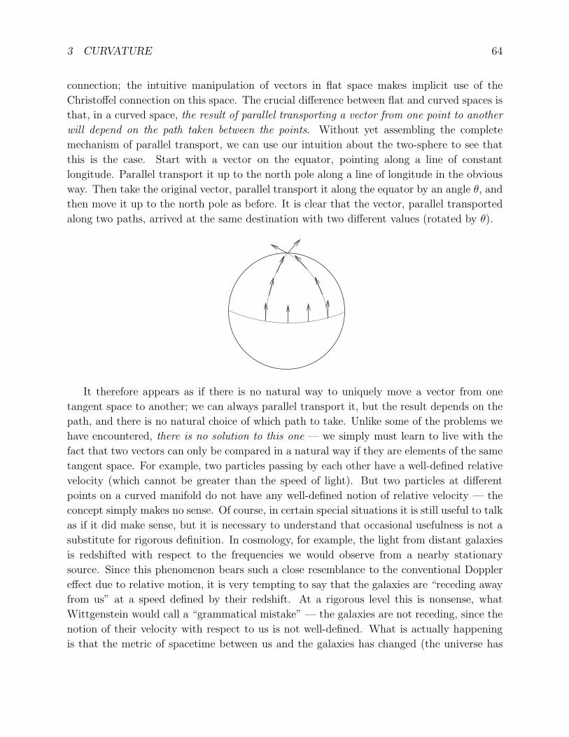
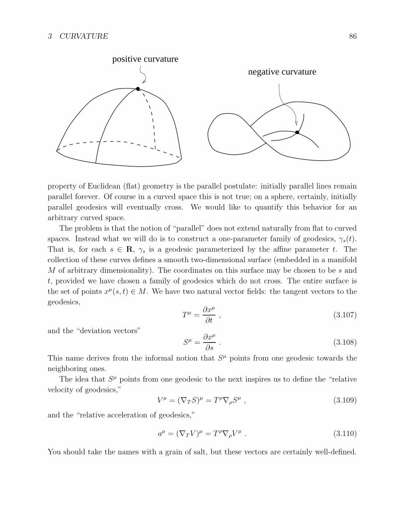
Notice that the Ricci scalar is not only constant for the two-sphere, it is manifestly
positive. We say that the sphere is “positively curved” (of course a convention or two came
into play, but fortunately our conventions conspired so that spaces which everyone agrees
to call positively curved actually have a positive Ricci scalar). From the point of view of
someone living on a manifold which is embedded in a higher-dimensional Euclidean space,
if they are sitting at a point of positive curvature the space curves away from them in the
same way in any direction, while in a negatively curved space it curves away in opposite
directions. Negatively curved spaces are therefore saddle-like.
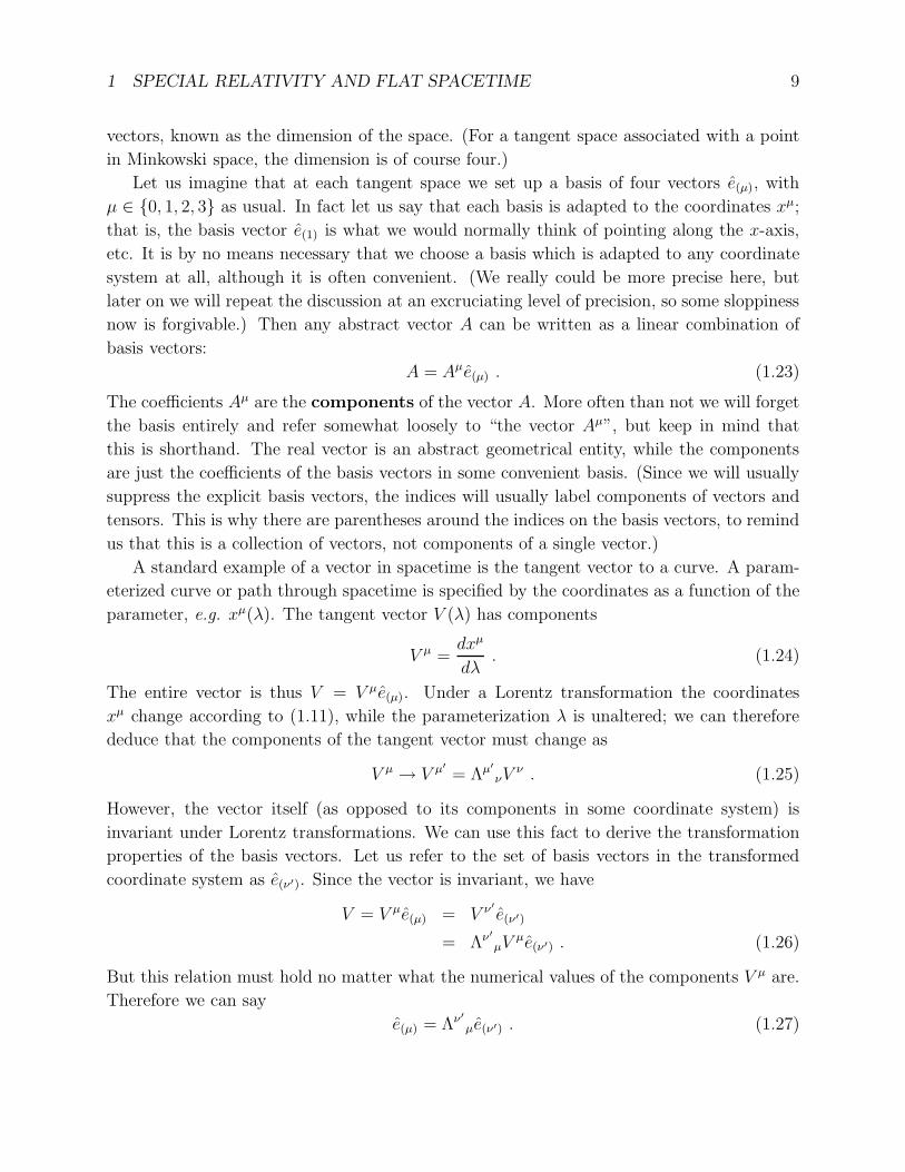
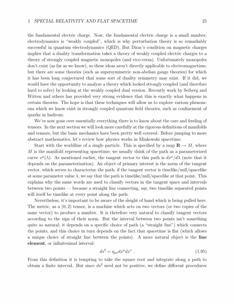
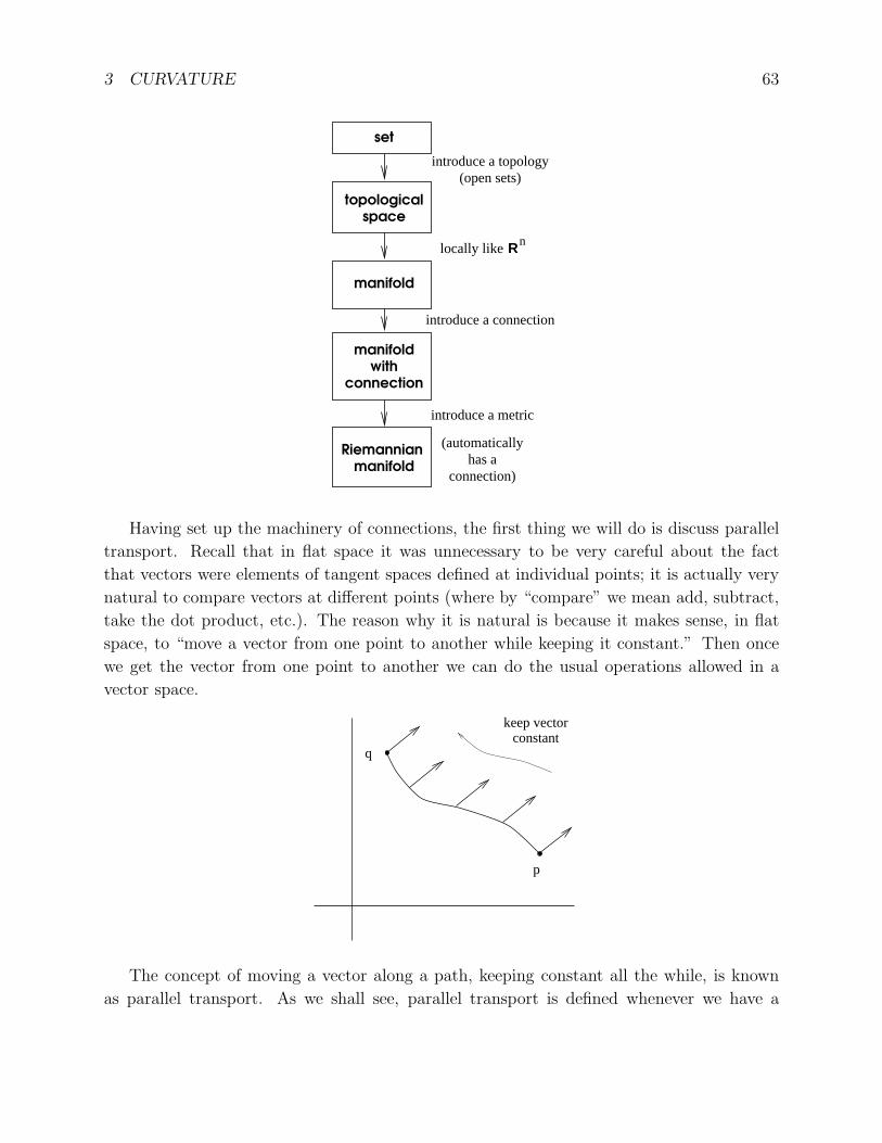
Enough fun with examples. There is one more topic we have to cover before introducing
general relativity itself: geodesic deviation. You have undoubtedly heard that the defining
3 CURVATURE 86
positive curvaturenegative curvature
property of Euclidean (flat) geometry is the parallel postulate: initially parallel lines remain
parallel forever. Of course in a curved space this is not true; on a sphere, certainly, initially
parallel geodesics will eventually cross. We would like to quantify this behavior for an
arbitrary curved space.
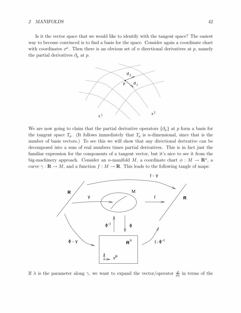
The problem is that the notion of “parallel” does not extend naturally from flat to curved
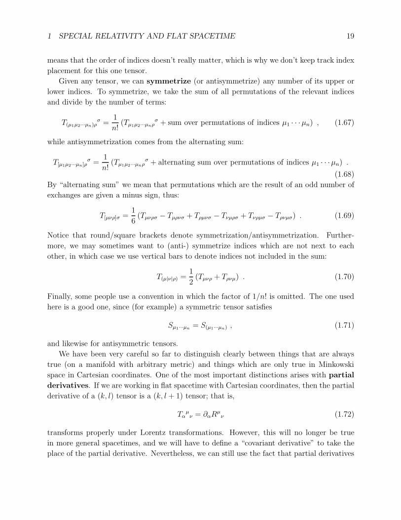
spaces. Instead what we will do is to construct a one-parameter family of geodesics, γs(t).
That is, for each s ∈ R, γs is a geodesic parameterized by the affine parameter t. The
collection of these curves defines a smooth two-dimensional surface (embedded in a manifold
M of arbitrary dimensionality). The coordinates on this surface may be chosen to be s and
t, provided we have chosen a family of geodesics which do not cross. The entire surface is
the set of points xµ(s, t) ∈M . We have two natural vector fields: the tangent vectors to the
geodesics,
T µ =∂xµ
∂t, (3.107)
and the “deviation vectors”
Sµ =∂xµ
∂s. (3.108)
This name derives from the informal notion that Sµ points from one geodesic towards the
neighboring ones.
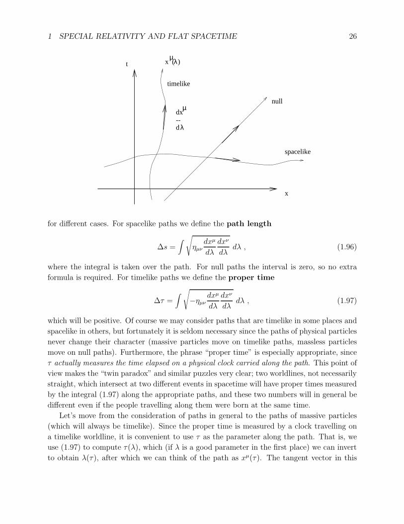
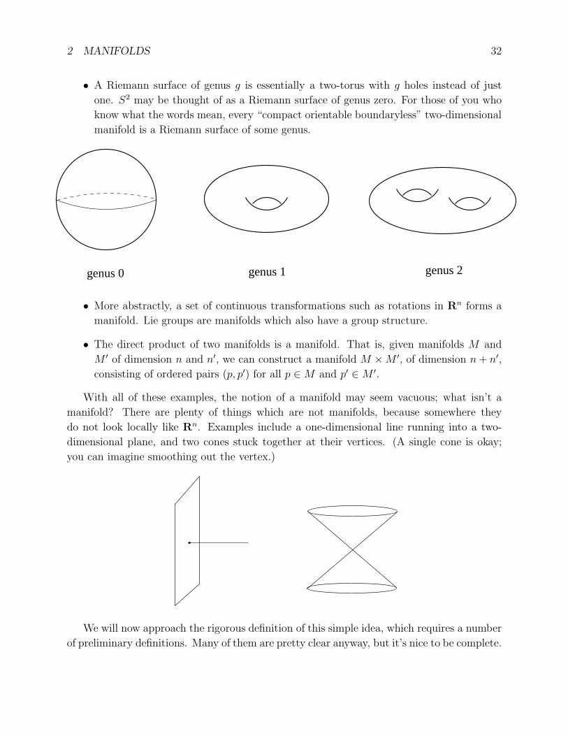
The idea that Sµ points from one geodesic to the next inspires us to define the “relative
velocity of geodesics,”
V µ = (∇TS)µ = T ρ∇ρSµ , (3.109)
and the “relative acceleration of geodesics,”
aµ = (∇TV )µ = T ρ∇ρVµ . (3.110)
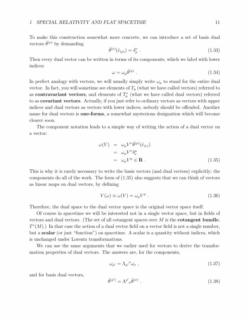
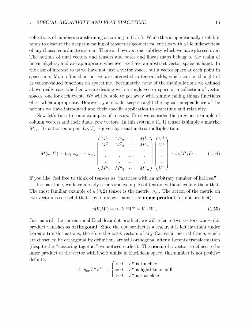
You should take the names with a grain of salt, but these vectors are certainly well-defined.
3 CURVATURE 87
t
s
T
S
γ ( )s tµ
µ
Since S and T are basis vectors adapted to a coordinate system, their commutator van-
ishes:
[S, T ] = 0 .
We would like to consider the conventional case where the torsion vanishes, so from (3.70)
we then have
Sρ∇ρTµ = T ρ∇ρS
µ . (3.111)
With this in mind, let’s compute the acceleration:
aµ = T ρ∇ρ(Tσ∇σS
µ)
= T ρ∇ρ(Sσ∇σT
µ)
= (T ρ∇ρSσ)(∇σT
µ) + T ρSσ∇ρ∇σTµ
= (Sρ∇ρTσ)(∇σT
µ) + T ρSσ(∇σ∇ρTµ +Rµ
νρσTν)
= (Sρ∇ρTσ)(∇σT
µ) + Sσ∇σ(T ρ∇ρTµ) − (Sσ∇σT
ρ)∇ρTµ +Rµ
νρσTνT ρSσ
= RµνρσT
νT ρSσ . (3.112)
Let’s think about this line by line. The first line is the definition of aµ, and the second
line comes directly from (3.111). The third line is simply the Leibniz rule. The fourth
line replaces a double covariant derivative by the derivatives in the opposite order plus the
Riemann tensor. In the fifth line we use Leibniz again (in the opposite order from usual),
and then we cancel two identical terms and notice that the term involving T ρ∇ρTµ vanishes
because T µ is the tangent vector to a geodesic. The result,
aµ =D2
dt2Sµ = Rµ
νρσTνT ρSσ , (3.113)
3 CURVATURE 88
is known as the geodesic deviation equation. It expresses something that we might have
expected: the relative acceleration between two neighboring geodesics is proportional to the
curvature.
Physically, of course, the acceleration of neighboring geodesics is interpreted as a mani-
festation of gravitational tidal forces. This reminds us that we are very close to doing physics
by now.
There is one last piece of formalism which it would be nice to cover before we move
on to gravitation proper. What we will do is to consider once again (although much more
concisely) the formalism of connections and curvature, but this time we will use sets of basis
vectors in the tangent space which are not derived from any coordinate system. It will turn
out that this slight change in emphasis reveals a different point of view on the connection
and curvature, one in which the relationship to gauge theories in particle physics is much
more transparent. In fact the concepts to be introduced are very straightforward, but the
subject is a notational nightmare, so it looks more difficult than it really is.
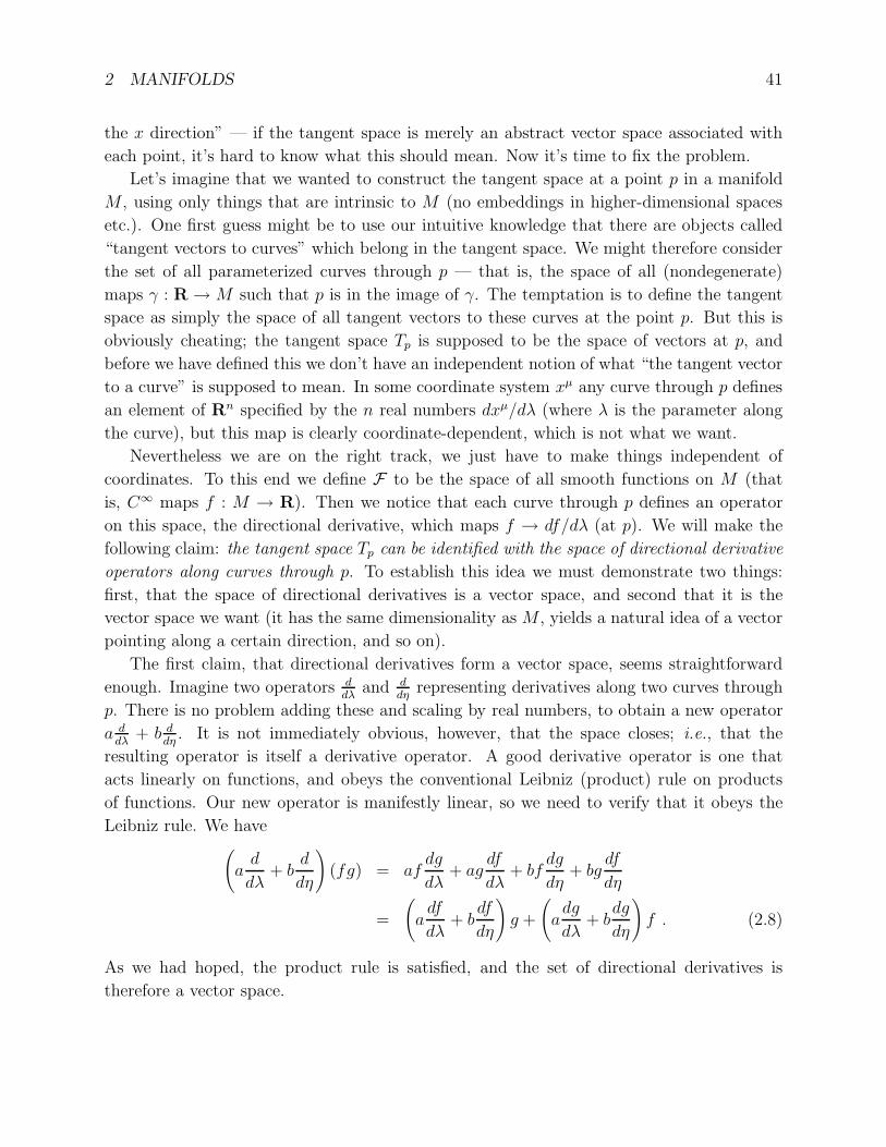
Up until now we have been taking advantage of the fact that a natural basis for the
tangent space Tp at a point p is given by the partial derivatives with respect to the coordinates
at that point, e(µ) = ∂µ. Similarly, a basis for the cotangent space T ∗p is given by the gradients
of the coordinate functions, θ(µ) = dxµ. There is nothing to stop us, however, from setting up
any bases we like. Let us therefore imagine that at each point in the manifold we introduce
a set of basis vectors e(a) (indexed by a Latin letter rather than Greek, to remind us that
they are not related to any coordinate system). We will choose these basis vectors to be
“orthonormal”, in a sense which is appropriate to the signature of the manifold we are
working on. That is, if the canonical form of the metric is written ηab, we demand that the
inner product of our basis vectors be
g(e(a), e(b)) = ηab , (3.114)
where g( , ) is the usual metric tensor. Thus, in a Lorentzian spacetime ηab represents
the Minkowski metric, while in a space with positive-definite metric it would represent the
Euclidean metric. The set of vectors comprising an orthonormal basis is sometimes known
as a tetrad (from Greek tetras, “a group of four”) or vielbein (from the German for “many
legs”). In different numbers of dimensions it occasionally becomes a vierbein (four), dreibein
(three), zweibein (two), and so on. (Just as we cannot in general find coordinate charts which
cover the entire manifold, we will often not be able to find a single set of smooth basis vector
fields which are defined everywhere. As usual, we can overcome this problem by working in
different patches and making sure things are well-behaved on the overlaps.)
The point of having a basis is that any vector can be expressed as a linear combination
of basis vectors. Specifically, we can express our old basis vectors e(µ) = ∂µ in terms of the
3 CURVATURE 89
new ones:
e(µ) = eaµe(a) . (3.115)
The components eaµ form an n × n invertible matrix. (In accord with our usual practice of
blurring the distinction between objects and their components, we will refer to the eaµ as
the tetrad or vielbein, and often in the plural as “vielbeins.”) We denote their inverse by
switching indices to obtain eµa , which satisfy
eµae
aν = δµ
ν , eaµe
µb = δa
b . (3.116)
These serve as the components of the vectors e(a) in the coordinate basis:
e(a) = eµa e(µ) . (3.117)
In terms of the inverse vielbeins, (3.114) becomes
gµνeµae
νb = ηab , (3.118)
or equivalently
gµν = eaµe
bνηab . (3.119)
This last equation sometimes leads people to say that the vielbeins are the “square root” of
the metric.
We can similarly set up an orthonormal basis of one-forms in T ∗p , which we denote θ(a).
They may be chosen to be compatible with the basis vectors, in the sense that
θ(a)(e(b)) = δab . (3.120)
It is an immediate consequence of this that the orthonormal one-forms are related to their
coordinate-based cousins θ(µ) = dxµ by
θ(µ) = eµa θ
(a) (3.121)
and
θ(a) = eaµθ
(µ) . (3.122)
The vielbeins eaµ thus serve double duty as the components of the coordinate basis vectors
in terms of the orthonormal basis vectors, and as components of the orthonormal basis
one-forms in terms of the coordinate basis one-forms; while the inverse vielbeins serve as
the components of the orthonormal basis vectors in terms of the coordinate basis, and as
components of the coordinate basis one-forms in terms of the orthonormal basis.
Any other vector can be expressed in terms of its components in the orthonormal basis.
If a vector V is written in the coordinate basis as V µe(µ) and in the orthonormal basis as
V ae(a), the sets of components will be related by
V a = eaµV
µ . (3.123)
3 CURVATURE 90
So the vielbeins allow us to “switch from Latin to Greek indices and back.” The nice property
of tensors, that there is usually only one sensible thing to do based on index placement, is
of great help here. We can go on to refer to multi-index tensors in either basis, or even in
terms of mixed components:
V ab = ea
µVµ
b = eνbV
aν = ea
µeνbV
µν . (3.124)
Looking back at (3.118), we see that the components of the metric tensor in the orthonormal
basis are just those of the flat metric, ηab. (For this reason the Greek indices are sometimes
referred to as “curved” and the Latin ones as “flat.”) In fact we can go so far as to raise and
lower the Latin indices using the flat metric and its inverse ηab. You can check for yourself
that everything works okay (e.g., that the lowering an index with the metric commutes with
changing from orthonormal to coordinate bases).
By introducing a new set of basis vectors and one-forms, we necessitate a return to our
favorite topic of transformation properties. We’ve been careful all along to emphasize that
the tensor transformation law was only an indirect outcome of a coordinate transformation;
the real issue was a change of basis. Now that we have non-coordinate bases, these bases can
be changed independently of the coordinates. The only restriction is that the orthonormality
property (3.114) be preserved. But we know what kind of transformations preserve the flat
metric — in a Euclidean signature metric they are orthogonal transformations, while in a
Lorentzian signature metric they are Lorentz transformations. We therefore consider changes
of basis of the form
e(a) → e(a′) = Λa′
a(x)e(a) , (3.125)
where the matrices Λa′a(x) represent position-dependent transformations which (at each
point) leave the canonical form of the metric unaltered:
Λa′
aΛb′bηab = ηa′b′ . (3.126)
In fact these matrices correspond to what in flat space we called the inverse Lorentz trans-
formations (which operate on basis vectors); as before we also have ordinary Lorentz trans-
formations Λa′
a, which transform the basis one-forms. As far as components are concerned,
as before we transform upper indices with Λa′
a and lower indices with Λa′a.
So we now have the freedom to perform a Lorentz transformation (or an ordinary Eu-
clidean rotation, depending on the signature) at every point in space. These transformations
are therefore called local Lorentz transformations, or LLT’s. We still have our usual
freedom to make changes in coordinates, which are called general coordinate trans-
formations, or GCT’s. Both can happen at the same time, resulting in a mixed tensor
transformation law:
T a′µ′
b′ν′ = Λa′
a∂xµ′
∂xµΛb′
b ∂xν
∂xν′T aµ
bν . (3.127)
3 CURVATURE 91
Translating what we know about tensors into non-coordinate bases is for the most part
merely a matter of sticking vielbeins in the right places. The crucial exception comes when
we begin to differentiate things. In our ordinary formalism, the covariant derivative of a
tensor is given by its partial derivative plus correction terms, one for each index, involving
the tensor and the connection coefficients. The same procedure will continue to be true
for the non-coordinate basis, but we replace the ordinary connection coefficients Γλµν by the
spin connection, denoted ωµab. Each Latin index gets a factor of the spin connection in
the usual way:
∇µXab = ∂µX
ab + ωµ
acX
cb − ωµ
cbX
ac . (3.128)
(The name “spin connection” comes from the fact that this can be used to take covari-
ant derivatives of spinors, which is actually impossible using the conventional connection
coefficients.) In the presence of mixed Latin and Greek indices we get terms of both kinds.
The usual demand that a tensor be independent of the way it is written allows us to
derive a relationship between the spin connection, the vielbeins, and the Γνµλ’s. Consider the
covariant derivative of a vector X, first in a purely coordinate basis:
∇X = (∇µXν)dxµ ⊗ ∂ν
= (∂µXν + Γν
µλXλ)dxµ ⊗ ∂ν . (3.129)
Now find the same object in a mixed basis, and convert into the coordinate basis:
∇X = (∇µXa)dxµ ⊗ e(a)
= (∂µXa + ωµ
abX
b)dxµ ⊗ e(a)
= (∂µ(eaνX
ν) + ωµabe
bλX
λ)dxµ ⊗ (eσa∂σ)
= eσa(ea
ν∂µXν +Xν∂µe
aν + ωµ
abe
bλX
λ)dxµ ⊗ ∂σ
= (∂µXν + eν
a∂µeaλX
λ + eνae
bλωµ
abX
λ)dxµ ⊗ ∂ν . (3.130)
Comparison with (3.129) reveals
Γνµλ = eν
a∂µeaλ + eν
aebλωµ
ab , (3.131)
or equivalently
ωµab = ea
νeλb Γ
νµλ − eλ
b∂µeaλ . (3.132)
A bit of manipulation allows us to write this relation as the vanishing of the covariant
derivative of the vielbein,
∇µeaν = 0 , (3.133)
which is sometimes known as the “tetrad postulate.” Note that this is always true; we did
not need to assume anything about the connection in order to derive it. Specifically, we did
not need to assume that the connection was metric compatible or torsion free.
3 CURVATURE 92
Since the connection may be thought of as something we need to fix up the transformation
law of the covariant derivative, it should come as no surprise that the spin connection does
not itself obey the tensor transformation law. Actually, under GCT’s the one lower Greek
index does transform in the right way, as a one-form. But under LLT’s the spin connection
transforms inhomogeneously, as
ωµa′
b′ = Λa′
aΛb′bωµ
ab − Λb′
c∂µΛa′
c . (3.134)
You are encouraged to check for yourself that this results in the proper transformation of
the covariant derivative.
So far we have done nothing but empty formalism, translating things we already knew
into a new notation. But the work we are doing does buy us two things. The first, which
we already alluded to, is the ability to describe spinor fields on spacetime and take their
covariant derivatives; we won’t explore this further right now. The second is a change in
viewpoint, in which we can think of various tensors as tensor-valued differential forms. For
example, an object like Xµa, which we think of as a (1, 1) tensor written with mixed indices,
can also be thought of as a “vector-valued one-form.” It has one lower Greek index, so we
think of it as a one-form, but for each value of the lower index it is a vector. Similarly a
tensor Aµνab, antisymmetric in µ and ν, can be thought of as a “(1, 1)-tensor-valued two-
form.” Thus, any tensor with some number of antisymmetric lower Greek indices and some
number of Latin indices can be thought of as a differential form, but taking values in the
tensor bundle. (Ordinary differential forms are simply scalar-valued forms.) The usefulness
of this viewpoint comes when we consider exterior derivatives. If we want to think of Xµa
as a vector-valued one-form, we are tempted to take its exterior derivative:
(dX)µνa = ∂µXν
a − ∂νXµa . (3.135)
It is easy to check that this object transforms like a two-form (that is, according to the
transformation law for (0, 2) tensors) under GCT’s, but not as a vector under LLT’s (the
Lorentz transformations depend on position, which introduces an inhomogeneous term into
the transformation law). But we can fix this by judicious use of the spin connection, which
can be thought of as a one-form. (Not a tensor-valued one-form, due to the nontensorial
transformation law (3.134).) Thus, the object
(dX)µνa + (ω ∧X)µν
a = ∂µXνa − ∂νXµ
a + ωµabXν
b − ωνabXµ
b , (3.136)
as you can verify at home, transforms as a proper tensor.
An immediate application of this formalism is to the expressions for the torsion and
curvature, the two tensors which characterize any given connection. The torsion, with two
antisymmetric lower indices, can be thought of as a vector-valued two-form Tµνa. The
3 CURVATURE 93
curvature, which is always antisymmetric in its last two indices, is a (1, 1)-tensor-valued
two-form, Rabµν . Using our freedom to suppress indices on differential forms, we can write
the defining relations for these two tensors as
T a = dea + ωab ∧ eb (3.137)
and
Rab = dωa
b + ωac ∧ ωc
b . (3.138)
These are known as the Maurer-Cartan structure equations. They are equivalent to
the usual definitions; let’s go through the exercise of showing this for the torsion, and you
can check the curvature for yourself. We have
Tµνλ = eλ
aTµνa
= eλa(∂µeν
a − ∂νeµa + ωµ
abeν
b − ωνabeµ
b)
= Γλµν − Γλ
νµ , (3.139)
which is just the original definition we gave. Here we have used (3.131), the expression for
the Γλµν ’s in terms of the vielbeins and spin connection. We can also express identities obeyed
by these tensors as
dT a + ωab ∧ T b = Ra
b ∧ eb (3.140)
and
dRab + ωa
c ∧ Rcb − Ra
c ∧ ωcb = 0 . (3.141)
The first of these is the generalization of Rρ[σµν] = 0, while the second is the Bianchi identity
∇[λ|Rρσ|µν] = 0. (Sometimes both equations are called Bianchi identities.)
The form of these expressions leads to an almost irresistible temptation to define a
“covariant-exterior derivative”, which acts on a tensor-valued form by taking the ordinary
exterior derivative and then adding appropriate terms with the spin connection, one for each
Latin index. Although we won’t do that here, it is okay to give in to this temptation, and
in fact the right hand side of (3.137) and the left hand sides of (3.140) and (3.141) can be
thought of as just such covariant-exterior derivatives. But be careful, since (3.138) cannot;
you can’t take any sort of covariant derivative of the spin connection, since it’s not a tensor.
So far our equations have been true for general connections; let’s see what we get for the
Christoffel connection. The torsion-free requirement is just that (3.137) vanish; this does
not lead immediately to any simple statement about the coefficients of the spin connection.
Metric compatibility is expressed as the vanishing of the covariant derivative of the metric:
∇g = 0. We can see what this leads to when we express the metric in the orthonormal basis,
where its components are simply ηab:
∇µηab = ∂µηab − ωµcaηcb − ωµ
cbηac
3 CURVATURE 94
= −ωµab − ωµba . (3.142)
Then setting this equal to zero implies
ωµab = −ωµba . (3.143)
Thus, metric compatibility is equivalent to the antisymmetry of the spin connection in its
Latin indices. (As before, such a statement is only sensible if both indices are either upstairs
or downstairs.) These two conditions together allow us to express the spin connection in
terms of the vielbeins. There is an explicit formula which expresses this solution, but in
practice it is easier to simply solve the torsion-free condition
ωab ∧ eb = −dea , (3.144)
using the asymmetry of the spin connection, to find the individual components.
We now have the means to compare the formalism of connections and curvature in Rie-
mannian geometry to that of gauge theories in particle physics. (This is an aside, which is
hopefully comprehensible to everybody, but not an essential ingredient of the course.) In
both situations, the fields of interest live in vector spaces which are assigned to each point
in spacetime. In Riemannian geometry the vector spaces include the tangent space, the
cotangent space, and the higher tensor spaces constructed from these. In gauge theories,
on the other hand, we are concerned with “internal” vector spaces. The distinction is that
the tangent space and its relatives are intimately associated with the manifold itself, and
were naturally defined once the manifold was set up; an internal vector space can be of any
dimension we like, and has to be defined as an independent addition to the manifold. In
math lingo, the union of the base manifold with the internal vector spaces (defined at each
point) is a fiber bundle, and each copy of the vector space is called the “fiber” (in perfect
accord with our definition of the tangent bundle).
Besides the base manifold (for us, spacetime) and the fibers, the other important ingre-
dient in the definition of a fiber bundle is the “structure group,” a Lie group which acts
on the fibers to describe how they are sewn together on overlapping coordinate patches.
Without going into details, the structure group for the tangent bundle in a four-dimensional
spacetime is generally GL(4,R), the group of real invertible 4 × 4 matrices; if we have a
Lorentzian metric, this may be reduced to the Lorentz group SO(3, 1). Now imagine that
we introduce an internal three-dimensional vector space, and sew the fibers together with
ordinary rotations; the structure group of this new bundle is then SO(3). A field that lives
in this bundle might be denoted φA(xµ), where A runs from one to three; it is a three-vector
(an internal one, unrelated to spacetime) for each point on the manifold. We have freedom
to choose the basis in the fibers in any way we wish; this means that “physical quantities”
should be left invariant under local SO(3) transformations such as
φA(xµ) → φA′
(xµ) = OA′
A(xµ)φA(xµ) , (3.145)
3 CURVATURE 95
where OA′
A(xµ) is a matrix in SO(3) which depends on spacetime. Such transformations
are known as gauge transformations, and theories invariant under them are called “gauge
theories.”
For the most part it is not hard to arrange things such that physical quantities are
invariant under gauge transformations. The one difficulty arises when we consider partial
derivatives, ∂µφA. Because the matrix OA′
A(xµ) depends on spacetime, it will contribute an
unwanted term to the transformation of the partial derivative. By now you should be able
to guess the solution: introduce a connection to correct for the inhomogeneous term in the
transformation law. We therefore define a connection on the fiber bundle to be an object
AµA
B, with two “group indices” and one spacetime index. Under GCT’s it transforms as a
one-form, while under gauge transformations it transforms as
AµA′
B′ = OA′
AOB′
BAµA
B − OB′
C∂µOA′
C . (3.146)
(Beware: our conventions are so drastically different from those in the particle physics liter-
ature that I won’t even try to get them straight.) With this transformation law, the “gauge
covariant derivative”
DµφA = ∂µφ
A + AµA
BφB (3.147)
transforms “tensorially” under gauge transformations, as you are welcome to check. (In
ordinary electromagnetism the connection is just the conventional vector potential. No
indices are necessary, because the structure group U(1) is one-dimensional.)
It is clear that this notion of a connection on an internal fiber bundle is very closely
related to the connection on the tangent bundle, especially in the orthonormal-frame picture
we have been discussing. The transformation law (3.146), for example, is exactly the same
as the transformation law (3.134) for the spin connection. We can also define a curvature or
“field strength” tensor which is a two-form,
FAB = dAA
B + AAC ∧ AC
B , (3.148)
in exact correspondence with (3.138). We can parallel transport things along paths, and
there is a construction analogous to the parallel propagator; the trace of the matrix obtained
by parallel transporting a vector around a closed curve is called a “Wilson loop.”
We could go on in the development of the relationship between the tangent bundle and
internal vector bundles, but time is short and we have other fish to fry. Let us instead finish
by emphasizing the important difference between the two constructions. The difference
stems from the fact that the tangent bundle is closely related to the base manifold, while
other fiber bundles are tacked on after the fact. It makes sense to say that a vector in the
tangent space at p “points along a path” through p; but this makes no sense for an internal
vector bundle. There is therefore no analogue of the coordinate basis for an internal space —
3 CURVATURE 96
partial derivatives along curves have nothing to do with internal vectors. It follows in turn
that there is nothing like the vielbeins, which relate orthonormal bases to coordinate bases.
The torsion tensor, in particular, is only defined for a connection on the tangent bundle, not
for any gauge theory connections; it can be thought of as the covariant exterior derivative
of the vielbein, and no such construction is available on an internal bundle. You should
appreciate the relationship between the different uses of the notion of a connection, without
getting carried away.
December 1997 Lecture Notes on General Relativity Sean M. Carroll
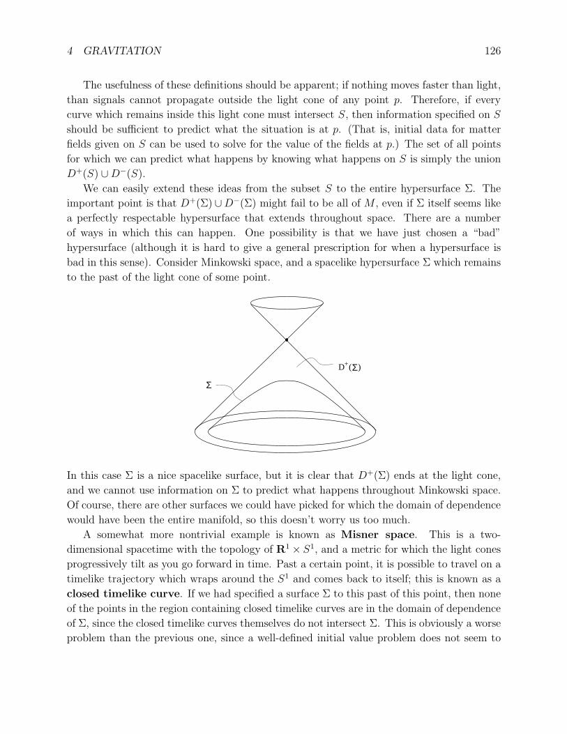
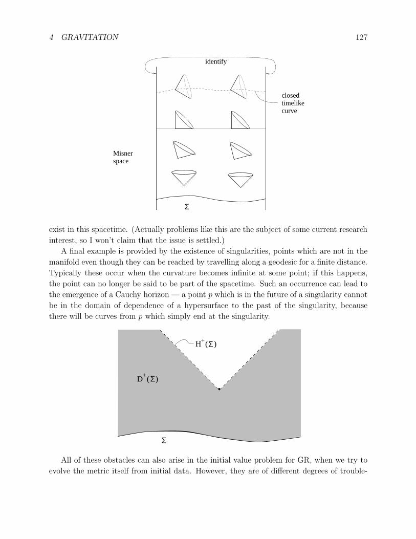
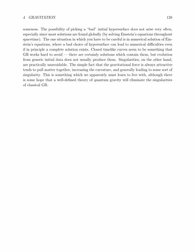
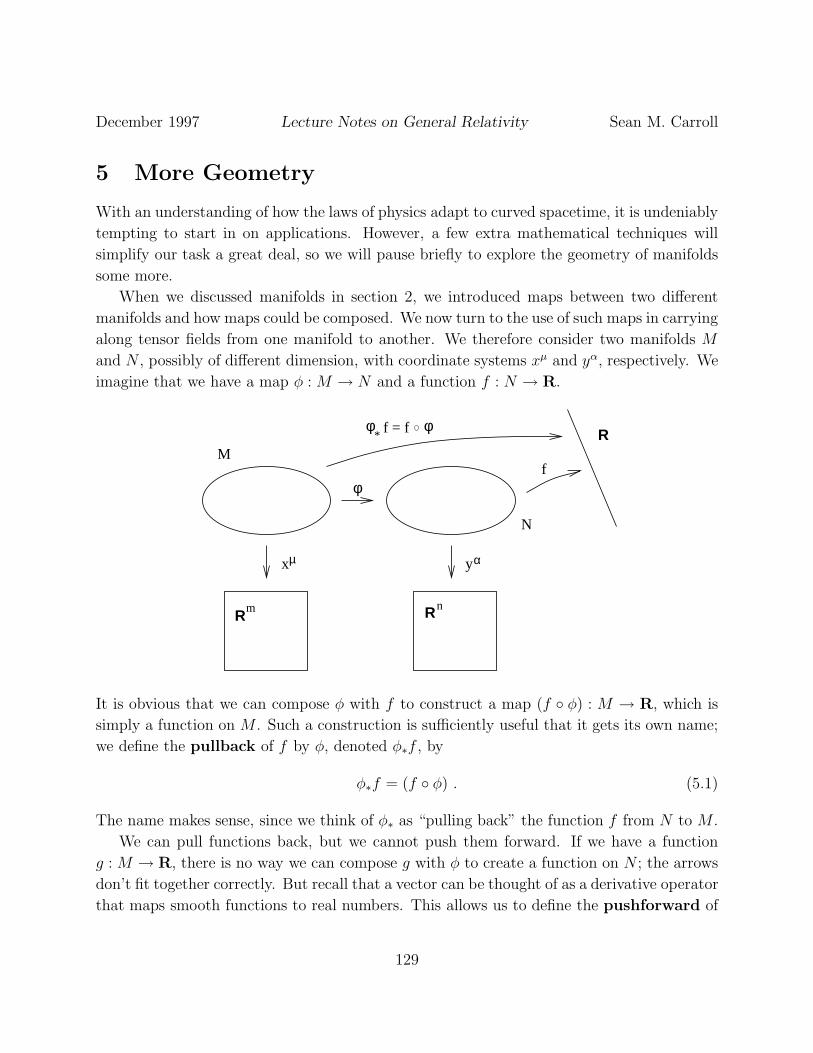
4 Gravitation
Having paid our mathematical dues, we are now prepared to examine the physics of gravita-
tion as described by general relativity. This subject falls naturally into two pieces: how the
curvature of spacetime acts on matter to manifest itself as “gravity”, and how energy and
momentum influence spacetime to create curvature. In either case it would be legitimate
to start at the top, by stating outright the laws governing physics in curved spacetime and
working out their consequences. Instead, we will try to be a little more motivational, starting
with basic physical principles and attempting to argue that these lead naturally to an almost
unique physical theory.
The most basic of these physical principles is the Principle of Equivalence, which comes
in a variety of forms. The earliest form dates from Galileo and Newton, and is known as
the Weak Equivalence Principle, or WEP. The WEP states that the “inertial mass” and
“gravitational mass” of any object are equal. To see what this means, think about Newton’s
Second Law. This relates the force exerted on an object to the acceleration it undergoes,
setting them proportional to each other with the constant of proportionality being the inertial
mass mi:
f = mia . (4.1)
The inertial mass clearly has a universal character, related to the resistance you feel when
you try to push on the object; it is the same constant no matter what kind of force is being
exerted. We also have the law of gravitation, which states that the gravitational force exerted
on an object is proportional to the gradient of a scalar field Φ, known as the gravitational
potential. The constant of proportionality in this case is called the gravitational mass mg:
fg = −mg∇Φ . (4.2)
On the face of it, mg has a very different character than mi; it is a quantity specific to the
gravitational force. If you like, it is the “gravitational charge” of the body. Nevertheless,
Galileo long ago showed (apocryphally by dropping weights off of the Leaning Tower of Pisa,
actually by rolling balls down inclined planes) that the response of matter to gravitation was
universal — every object falls at the same rate in a gravitational field, independent of the
composition of the object. In Newtonian mechanics this translates into the WEP, which is
simply
mi = mg (4.3)
for any object. An immediate consequence is that the behavior of freely-falling test particles
is universal, independent of their mass (or any other qualities they may have); in fact we
97
4 GRAVITATION 98
have
a = −∇Φ . (4.4)
The universality of gravitation, as implied by the WEP, can be stated in another, more
popular, form. Imagine that we consider a physicist in a tightly sealed box, unable to
observe the outside world, who is doing experiments involving the motion of test particles,
for example to measure the local gravitational field. Of course she would obtain different
answers if the box were sitting on the moon or on Jupiter than she would on the Earth.
But the answers would also be different if the box were accelerating at a constant velocity;
this would change the acceleration of the freely-falling particles with respect to the box.
The WEP implies that there is no way to disentangle the effects of a gravitational field
from those of being in a uniformly accelerating frame, simply by observing the behavior of
freely-falling particles. This follows from the universality of gravitation; it would be possible
to distinguish between uniform acceleration and an electromagnetic field, by observing the
behavior of particles with different charges. But with gravity it is impossible, since the
“charge” is necessarily proportional to the (inertial) mass.
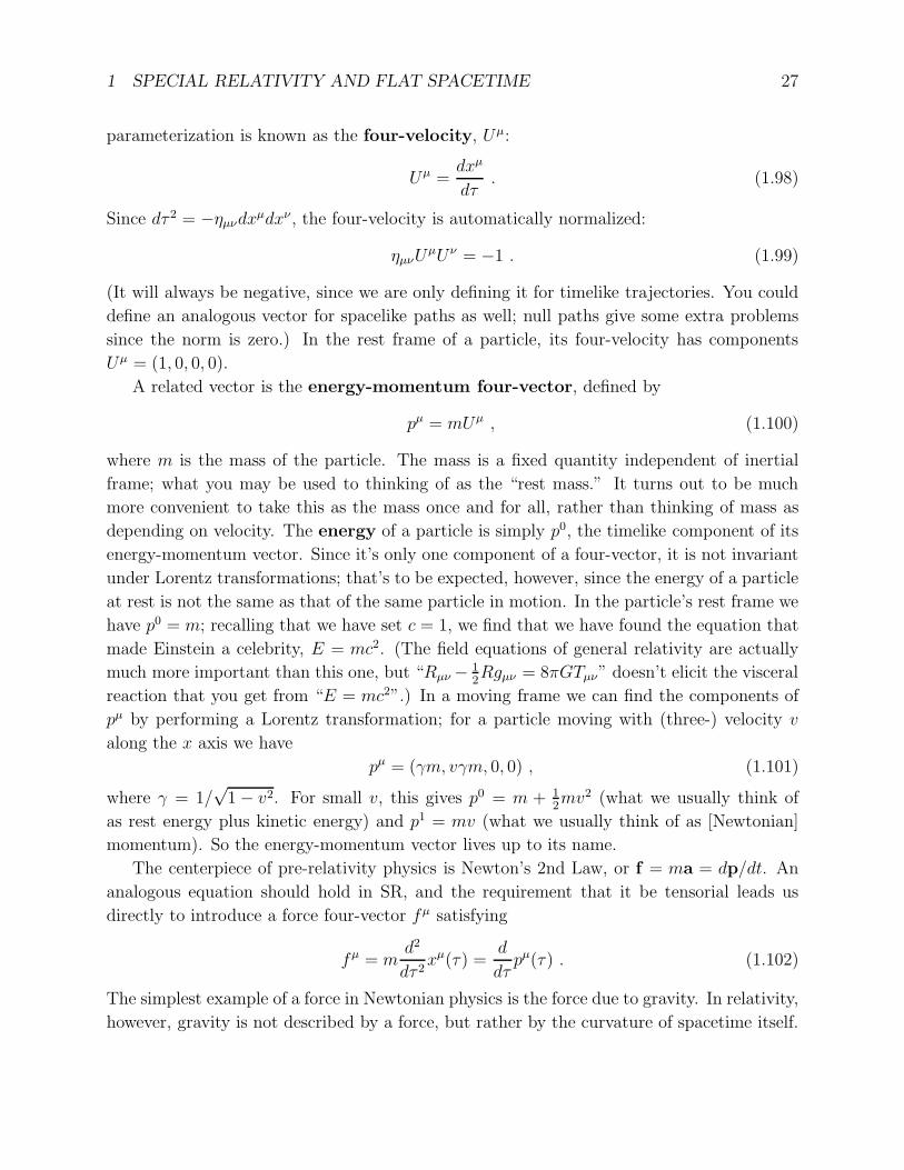
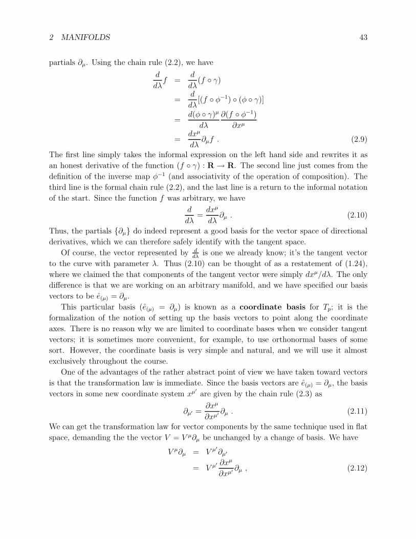
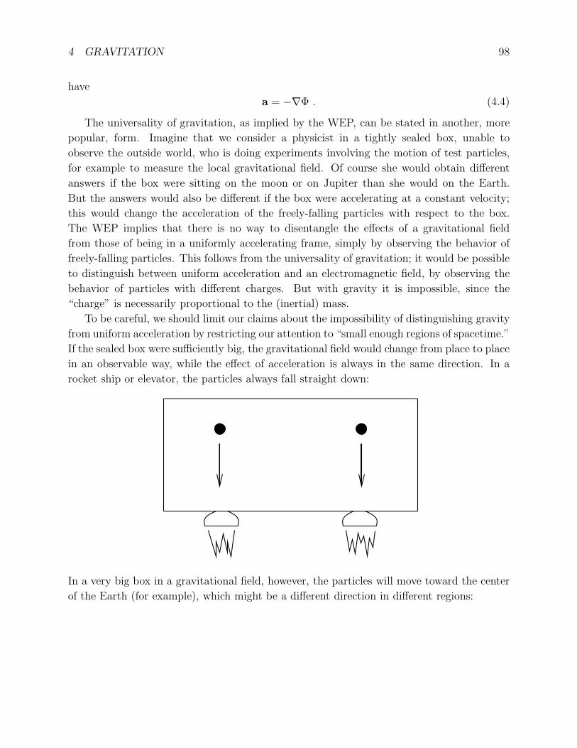
To be careful, we should limit our claims about the impossibility of distinguishing gravity
from uniform acceleration by restricting our attention to “small enough regions of spacetime.”
If the sealed box were sufficiently big, the gravitational field would change from place to place
in an observable way, while the effect of acceleration is always in the same direction. In a
rocket ship or elevator, the particles always fall straight down:
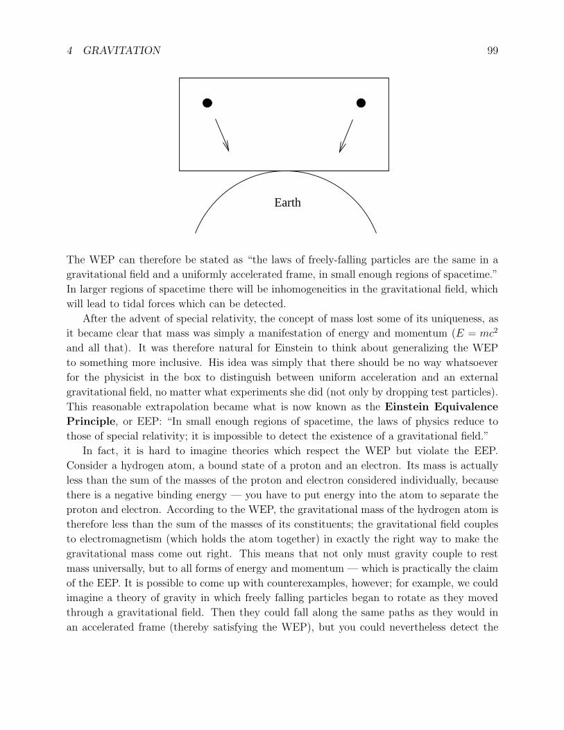
In a very big box in a gravitational field, however, the particles will move toward the center
of the Earth (for example), which might be a different direction in different regions:
4 GRAVITATION 99
Earth
The WEP can therefore be stated as “the laws of freely-falling particles are the same in a
gravitational field and a uniformly accelerated frame, in small enough regions of spacetime.”
In larger regions of spacetime there will be inhomogeneities in the gravitational field, which
will lead to tidal forces which can be detected.
After the advent of special relativity, the concept of mass lost some of its uniqueness, as
it became clear that mass was simply a manifestation of energy and momentum (E = mc2
and all that). It was therefore natural for Einstein to think about generalizing the WEP
to something more inclusive. His idea was simply that there should be no way whatsoever
for the physicist in the box to distinguish between uniform acceleration and an external
gravitational field, no matter what experiments she did (not only by dropping test particles).
This reasonable extrapolation became what is now known as the Einstein Equivalence
Principle, or EEP: “In small enough regions of spacetime, the laws of physics reduce to
those of special relativity; it is impossible to detect the existence of a gravitational field.”
In fact, it is hard to imagine theories which respect the WEP but violate the EEP.
Consider a hydrogen atom, a bound state of a proton and an electron. Its mass is actually
less than the sum of the masses of the proton and electron considered individually, because
there is a negative binding energy — you have to put energy into the atom to separate the
proton and electron. According to the WEP, the gravitational mass of the hydrogen atom is
therefore less than the sum of the masses of its constituents; the gravitational field couples
to electromagnetism (which holds the atom together) in exactly the right way to make the
gravitational mass come out right. This means that not only must gravity couple to rest
mass universally, but to all forms of energy and momentum — which is practically the claim
of the EEP. It is possible to come up with counterexamples, however; for example, we could
imagine a theory of gravity in which freely falling particles began to rotate as they moved
through a gravitational field. Then they could fall along the same paths as they would in
an accelerated frame (thereby satisfying the WEP), but you could nevertheless detect the
4 GRAVITATION 100
existence of the gravitational field (in violation of the EEP). Such theories seem contrived,
but there is no law of nature which forbids them.
Sometimes a distinction is drawn between “gravitational laws of physics” and “non-
gravitational laws of physics,” and the EEP is defined to apply only to the latter. Then
one defines the “Strong Equivalence Principle” (SEP) to include all of the laws of physics,
gravitational and otherwise. I don’t find this a particularly useful distinction, and won’t
belabor it. For our purposes, the EEP (or simply “the principle of equivalence”) includes all
of the laws of physics.
It is the EEP which implies (or at least suggests) that we should attribute the action
of gravity to the curvature of spacetime. Remember that in special relativity a prominent
role is played by inertial frames — while it was not possible to single out some frame of
reference as uniquely “at rest”, it was possible to single out a family of frames which were
“unaccelerated” (inertial). The acceleration of a charged particle in an electromagnetic field
was therefore uniquely defined with respect to these frames. The EEP, on the other hand,
implies that gravity is inescapable — there is no such thing as a “gravitationally neutral
object” with respect to which we can measure the acceleration due to gravity. It follows
that “the acceleration due to gravity” is not something which can be reliably defined, and
therefore is of little use.
Instead, it makes more sense to define “unaccelerated” as “freely falling,” and that is
what we shall do. This point of view is the origin of the idea that gravity is not a “force”
— a force is something which leads to acceleration, and our definition of zero acceleration is
“moving freely in the presence of whatever gravitational field happens to be around.”
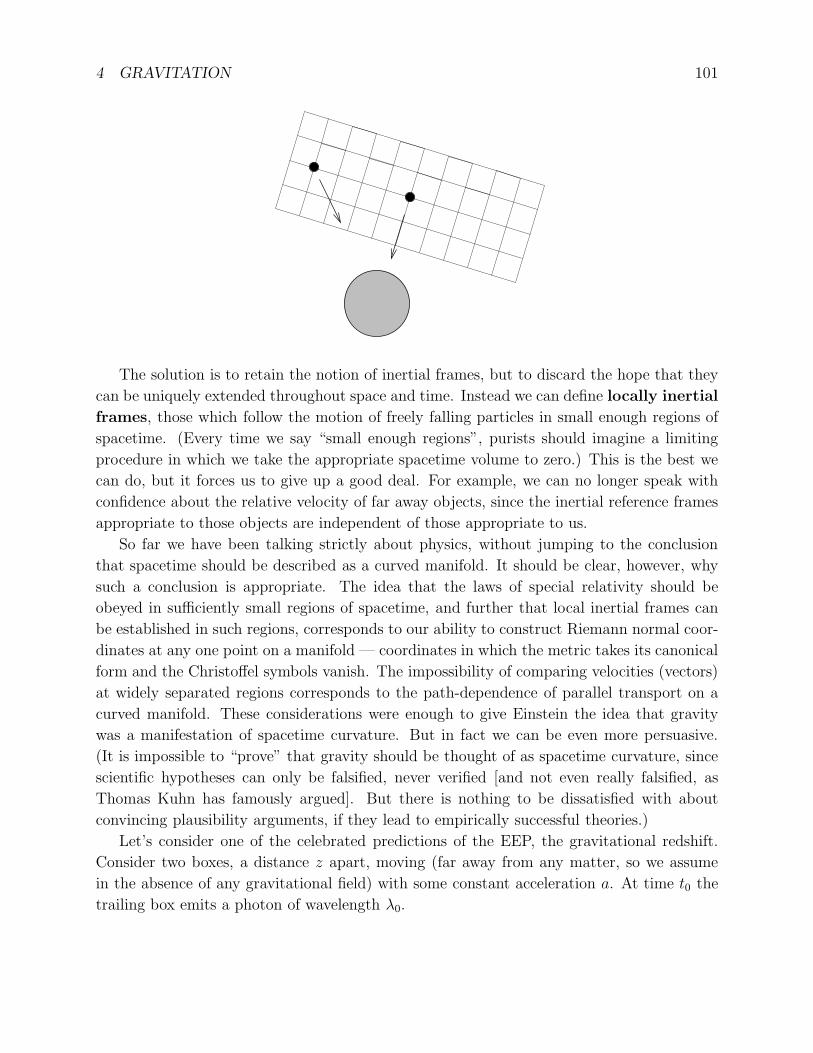
This seemingly innocuous step has profound implications for the nature of spacetime. In
SR, we had a procedure for starting at some point and constructing an inertial frame which
stretched throughout spacetime, by joining together rigid rods and attaching clocks to them.
But, again due to inhomogeneities in the gravitational field, this is no longer possible. If
we start in some freely-falling state and build a large structure out of rigid rods, at some
distance away freely-falling objects will look like they are “accelerating” with respect to this
reference frame, as shown in the figure on the next page.
4 GRAVITATION 101
The solution is to retain the notion of inertial frames, but to discard the hope that they
can be uniquely extended throughout space and time. Instead we can define locally inertial
frames, those which follow the motion of freely falling particles in small enough regions of
spacetime. (Every time we say “small enough regions”, purists should imagine a limiting
procedure in which we take the appropriate spacetime volume to zero.) This is the best we
can do, but it forces us to give up a good deal. For example, we can no longer speak with
confidence about the relative velocity of far away objects, since the inertial reference frames
appropriate to those objects are independent of those appropriate to us.
So far we have been talking strictly about physics, without jumping to the conclusion
that spacetime should be described as a curved manifold. It should be clear, however, why
such a conclusion is appropriate. The idea that the laws of special relativity should be
obeyed in sufficiently small regions of spacetime, and further that local inertial frames can
be established in such regions, corresponds to our ability to construct Riemann normal coor-
dinates at any one point on a manifold — coordinates in which the metric takes its canonical
form and the Christoffel symbols vanish. The impossibility of comparing velocities (vectors)
at widely separated regions corresponds to the path-dependence of parallel transport on a
curved manifold. These considerations were enough to give Einstein the idea that gravity
was a manifestation of spacetime curvature. But in fact we can be even more persuasive.
(It is impossible to “prove” that gravity should be thought of as spacetime curvature, since
scientific hypotheses can only be falsified, never verified [and not even really falsified, as
Thomas Kuhn has famously argued]. But there is nothing to be dissatisfied with about
convincing plausibility arguments, if they lead to empirically successful theories.)
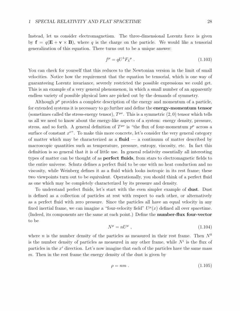
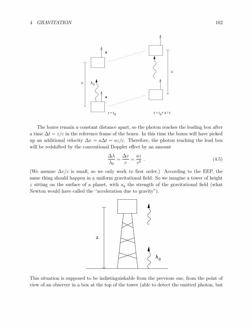
Let’s consider one of the celebrated predictions of the EEP, the gravitational redshift.
Consider two boxes, a distance z apart, moving (far away from any matter, so we assume
in the absence of any gravitational field) with some constant acceleration a. At time t0 the
trailing box emits a photon of wavelength λ0.
4 GRAVITATION 102
z
z
t = t t = t + z / c
a
a
0 0
λ0
The boxes remain a constant distance apart, so the photon reaches the leading box after
a time ∆t = z/c in the reference frame of the boxes. In this time the boxes will have picked
up an additional velocity ∆v = a∆t = az/c. Therefore, the photon reaching the lead box
will be redshifted by the conventional Doppler effect by an amount
∆λ
λ0=
∆v
c=az
c2. (4.5)
(We assume ∆v/c is small, so we only work to first order.) According to the EEP, the
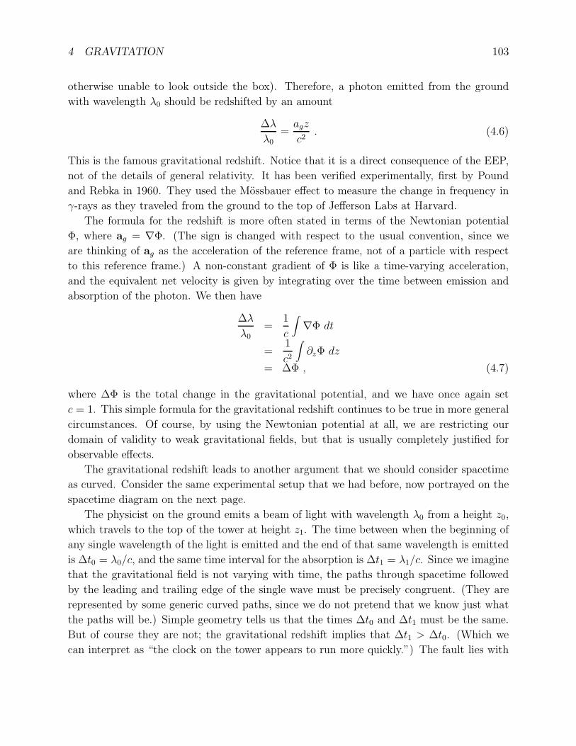
same thing should happen in a uniform gravitational field. So we imagine a tower of height
z sitting on the surface of a planet, with ag the strength of the gravitational field (what
Newton would have called the “acceleration due to gravity”).
λ0
z
This situation is supposed to be indistinguishable from the previous one, from the point of
view of an observer in a box at the top of the tower (able to detect the emitted photon, but
4 GRAVITATION 103
otherwise unable to look outside the box). Therefore, a photon emitted from the ground
with wavelength λ0 should be redshifted by an amount
∆λ
λ0=agz
c2. (4.6)
This is the famous gravitational redshift. Notice that it is a direct consequence of the EEP,
not of the details of general relativity. It has been verified experimentally, first by Pound
and Rebka in 1960. They used the Mossbauer effect to measure the change in frequency in
γ-rays as they traveled from the ground to the top of Jefferson Labs at Harvard.
The formula for the redshift is more often stated in terms of the Newtonian potential
Φ, where ag = ∇Φ. (The sign is changed with respect to the usual convention, since we
are thinking of ag as the acceleration of the reference frame, not of a particle with respect
to this reference frame.) A non-constant gradient of Φ is like a time-varying acceleration,
and the equivalent net velocity is given by integrating over the time between emission and
absorption of the photon. We then have
∆λ
λ0
=1
c
∫∇Φ dt
=1
c2
∫∂zΦ dz
= ∆Φ , (4.7)
where ∆Φ is the total change in the gravitational potential, and we have once again set
c = 1. This simple formula for the gravitational redshift continues to be true in more general
circumstances. Of course, by using the Newtonian potential at all, we are restricting our
domain of validity to weak gravitational fields, but that is usually completely justified for
observable effects.
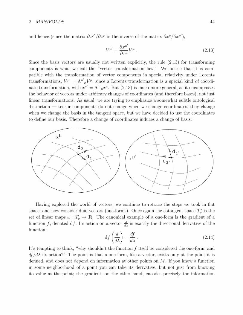
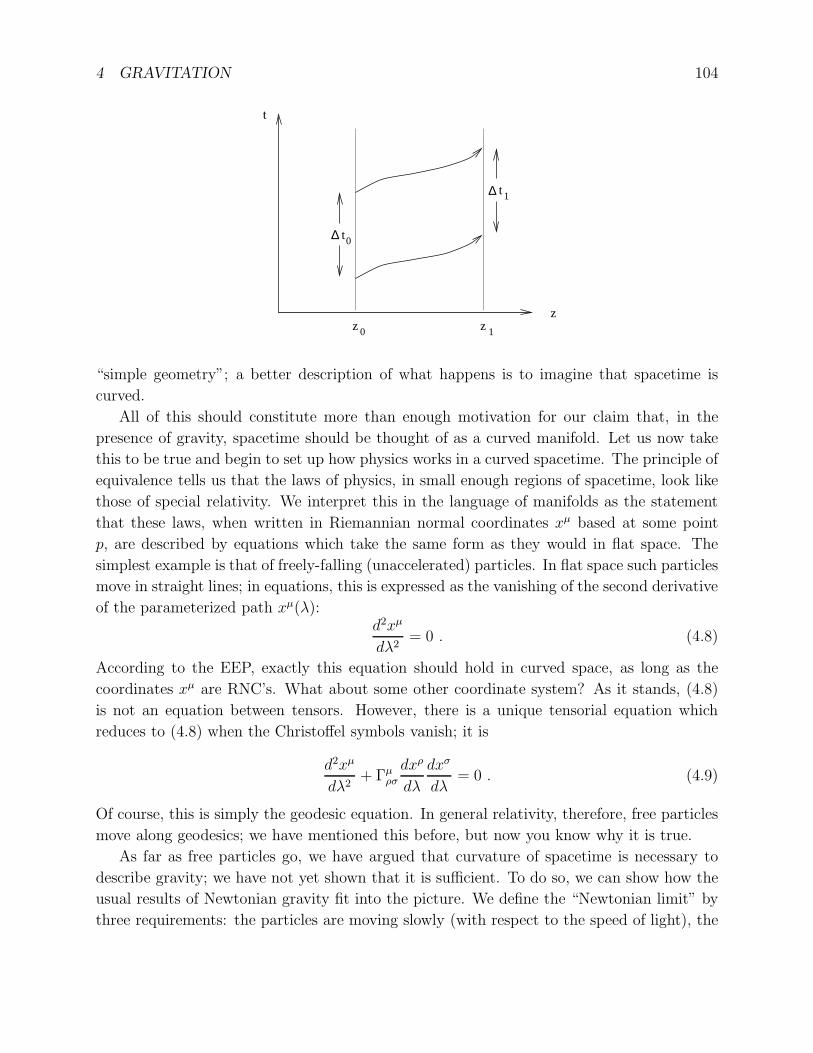
The gravitational redshift leads to another argument that we should consider spacetime
as curved. Consider the same experimental setup that we had before, now portrayed on the
spacetime diagram on the next page.
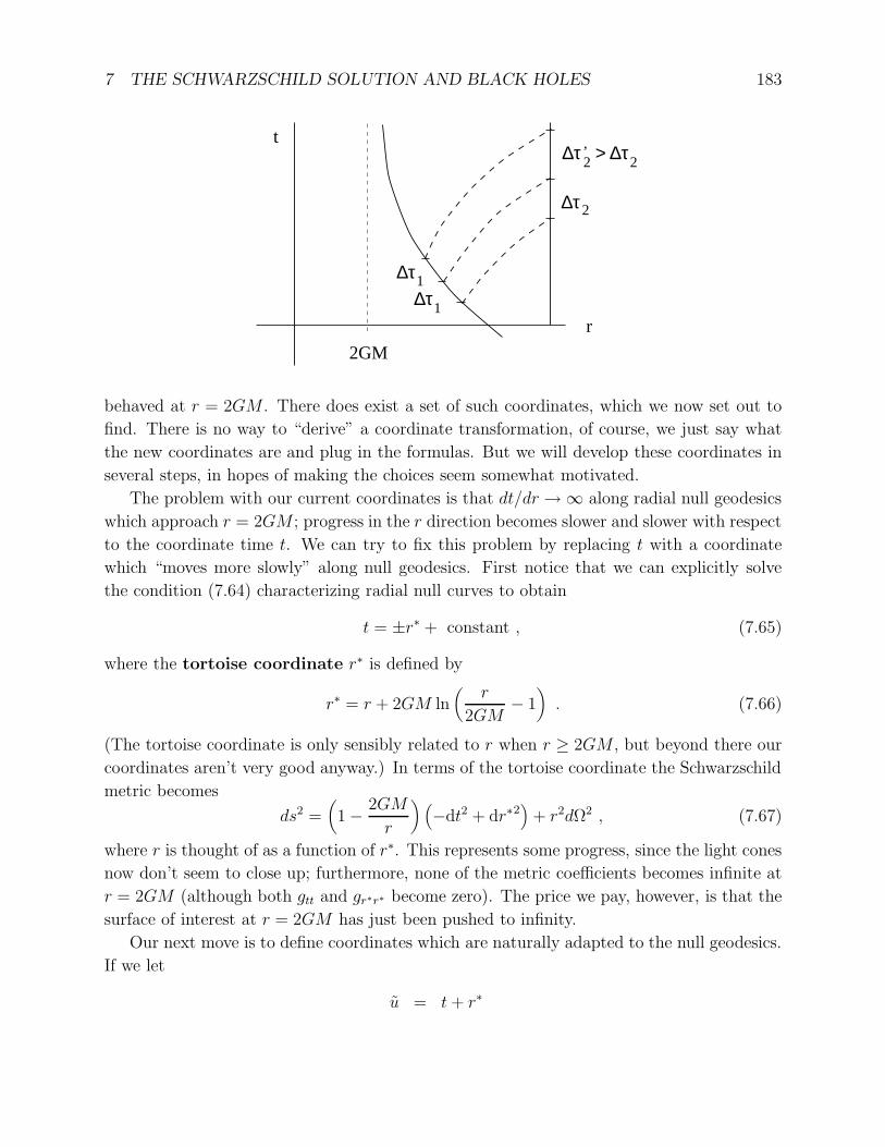
The physicist on the ground emits a beam of light with wavelength λ0 from a height z0,
which travels to the top of the tower at height z1. The time between when the beginning of
any single wavelength of the light is emitted and the end of that same wavelength is emitted
is ∆t0 = λ0/c, and the same time interval for the absorption is ∆t1 = λ1/c. Since we imagine
that the gravitational field is not varying with time, the paths through spacetime followed
by the leading and trailing edge of the single wave must be precisely congruent. (They are
represented by some generic curved paths, since we do not pretend that we know just what
the paths will be.) Simple geometry tells us that the times ∆t0 and ∆t1 must be the same.
But of course they are not; the gravitational redshift implies that ∆t1 > ∆t0. (Which we
can interpret as “the clock on the tower appears to run more quickly.”) The fault lies with
4 GRAVITATION 104
z zz
t
t∆ 0
∆ t 1
0 1
“simple geometry”; a better description of what happens is to imagine that spacetime is
curved.
All of this should constitute more than enough motivation for our claim that, in the
presence of gravity, spacetime should be thought of as a curved manifold. Let us now take
this to be true and begin to set up how physics works in a curved spacetime. The principle of
equivalence tells us that the laws of physics, in small enough regions of spacetime, look like
those of special relativity. We interpret this in the language of manifolds as the statement
that these laws, when written in Riemannian normal coordinates xµ based at some point
p, are described by equations which take the same form as they would in flat space. The
simplest example is that of freely-falling (unaccelerated) particles. In flat space such particles
move in straight lines; in equations, this is expressed as the vanishing of the second derivative
of the parameterized path xµ(λ):d2xµ
dλ2= 0 . (4.8)
According to the EEP, exactly this equation should hold in curved space, as long as the
coordinates xµ are RNC’s. What about some other coordinate system? As it stands, (4.8)
is not an equation between tensors. However, there is a unique tensorial equation which
reduces to (4.8) when the Christoffel symbols vanish; it is
d2xµ
dλ2+ Γµ
ρσ
dxρ
dλ
dxσ
dλ= 0 . (4.9)
Of course, this is simply the geodesic equation. In general relativity, therefore, free particles
move along geodesics; we have mentioned this before, but now you know why it is true.
As far as free particles go, we have argued that curvature of spacetime is necessary to
describe gravity; we have not yet shown that it is sufficient. To do so, we can show how the
usual results of Newtonian gravity fit into the picture. We define the “Newtonian limit” by
three requirements: the particles are moving slowly (with respect to the speed of light), the
4 GRAVITATION 105
gravitational field is weak (can be considered a perturbation of flat space), and the field is
also static (unchanging with time). Let us see what these assumptions do to the geodesic
equation, taking the proper time τ as an affine parameter. “Moving slowly” means that
dxi
dτ<<
dt
dτ, (4.10)
so the geodesic equation becomes
d2xµ
dτ 2+ Γµ
00
(dt
dτ
)2
= 0 . (4.11)
Since the field is static, the relevant Christoffel symbols Γµ00 simplify:
Γµ00 =
1
2gµλ(∂0gλ0 + ∂0g0λ − ∂λg00)
= −1
2gµλ∂λg00 . (4.12)
Finally, the weakness of the gravitational field allows us to decompose the metric into the
Minkowski form plus a small perturbation:
gµν = ηµν + hµν , |hµν | << 1 . (4.13)
(We are working in Cartesian coordinates, so ηµν is the canonical form of the metric. The
“smallness condition” on the metric perturbation hµν doesn’t really make sense in other
coordinates.) From the definition of the inverse metric, gµνgνσ = δµσ , we find that to first
order in h,
gµν = ηµν − hµν , (4.14)
where hµν = ηµρηνσhρσ. In fact, we can use the Minkowski metric to raise and lower indices
on an object of any definite order in h, since the corrections would only contribute at higher
orders.
Putting it all together, we find
Γµ00 = −1
2ηµλ∂λh00 . (4.15)
The geodesic equation (4.11) is therefore
d2xµ
dτ 2=
1
2ηµλ∂λh00
(dt
dτ
)2
. (4.16)
Using ∂0h00 = 0, the µ = 0 component of this is just
d2t
dτ 2= 0 . (4.17)
4 GRAVITATION 106
That is, dtdτ
is constant. To examine the spacelike components of (4.16), recall that the
spacelike components of ηµν are just those of a 3 × 3 identity matrix. We therefore have
d2xi
dτ 2=
1
2
(dt
dτ
)2
∂ih00 . (4.18)
Dividing both sides by(
dtdτ
)2has the effect of converting the derivative on the left-hand side
from τ to t, leaving us withd2xi
dt2=
1
2∂ih00 . (4.19)
This begins to look a great deal like Newton’s theory of gravitation. In fact, if we compare
this equation to (4.4), we find that they are the same once we identify
h00 = −2Φ , (4.20)
or in other words
g00 = −(1 + 2Φ) . (4.21)
Therefore, we have shown that the curvature of spacetime is indeed sufficient to describe
gravity in the Newtonian limit, as long as the metric takes the form (4.21). It remains, of
course, to find field equations for the metric which imply that this is the form taken, and
that for a single gravitating body we recover the Newtonian formula
Φ = −GMr
, (4.22)
but that will come soon enough.
Our next task is to show how the remaining laws of physics, beyond those governing freely-
falling particles, adapt to the curvature of spacetime. The procedure essentially follows the
paradigm established in arguing that free particles move along geodesics. Take a law of
physics in flat space, traditionally written in terms of partial derivatives and the flat metric.
According to the equivalence principle this law will hold in the presence of gravity, as long
as we are in Riemannian normal coordinates. Translate the law into a relationship between
tensors; for example, change partial derivatives to covariant ones. In RNC’s this version of
the law will reduce to the flat-space one, but tensors are coordinate-independent objects, so
the tensorial version must hold in any coordinate system.
This procedure is sometimes given a name, the Principle of Covariance. I’m not
sure that it deserves its own name, since it’s really a consequence of the EEP plus the
requirement that the laws of physics be independent of coordinates. (The requirement that
laws of physics be independent of coordinates is essentially impossible to even imagine being
untrue. Given some experiment, if one person uses one coordinate system to predict a result
and another one uses a different coordinate system, they had better agree.) Another name
4 GRAVITATION 107
is the “comma-goes-to-semicolon rule”, since at a typographical level the thing you have to
do is replace partial derivatives (commas) with covariant ones (semicolons).
We have already implicitly used the principle of covariance (or whatever you want to
call it) in deriving the statement that free particles move along geodesics. For the most
part, it is very simple to apply it to interesting cases. Consider for example the formula for
conservation of energy in flat spacetime, ∂µTµν = 0. The adaptation to curved spacetime is
immediate:
∇µTµν = 0 . (4.23)
This equation expresses the conservation of energy in the presence of a gravitational field.
Unfortunately, life is not always so easy. Consider Maxwell’s equations in special relativ-
ity, where it would seem that the principle of covariance can be applied in a straightforward
way. The inhomogeneous equation ∂µFνµ = 4πJν becomes
∇µFνµ = 4πJν , (4.24)
and the homogeneous one ∂[µFνλ] = 0 becomes
∇[µFνλ] = 0 . (4.25)
On the other hand, we could also write Maxwell’s equations in flat space in terms of differ-
ential forms as
d(∗F ) = 4π(∗J) , (4.26)
and
dF = 0 . (4.27)
These are already in perfectly tensorial form, since we have shown that the exterior derivative
is a well-defined tensor operator regardless of what the connection is. We therefore begin
to worry a little bit; what is the guarantee that the process of writing a law of physics in
tensorial form gives a unique answer? In fact, as we have mentioned earlier, the differential
forms versions of Maxwell’s equations should be taken as fundamental. Nevertheless, in this
case it happens to make no difference, since in the absence of torsion (4.26) is identical
to (4.24), and (4.27) is identical to (4.25); the symmetric part of the connection doesn’t
contribute. Similarly, the definition of the field strength tensor in terms of the potential Aµ
can be written either as
Fµν = ∇µAν −∇νAµ , (4.28)
or equally well as
F = dA . (4.29)
The worry about uniqueness is a real one, however. Imagine that two vector fields Xµ
and Y ν obey a law in flat space given by
Y µ∂µ∂νXν = 0 . (4.30)
4 GRAVITATION 108
The problem in writing this as a tensor equation should be clear: the partial derivatives can
be commuted, but covariant derivatives cannot. If we simply replace the partials in (4.30)
by covariant derivatives, we get a different answer than we would if we had first exchanged
the order of the derivatives (leaving the equation in flat space invariant) and then replaced
them. The difference is given by
Y µ∇µ∇νXν − Y µ∇ν∇µX
ν = −RµνYµXν . (4.31)
The prescription for generalizing laws from flat to curved spacetimes does not guide us in
choosing the order of the derivatives, and therefore is ambiguous about whether a term
such as that in (4.31) should appear in the presence of gravity. (The problem of ordering
covariant derivatives is similar to the problem of operator-ordering ambiguities in quantum
mechanics.)
In the literature you can find various prescriptions for dealing with ambiguities such as
this, most of which are sensible pieces of advice such as remembering to preserve gauge
invariance for electromagnetism. But deep down the real answer is that there is no way to
resolve these problems by pure thought alone; the fact is that there may be more than one
way to adapt a law of physics to curved space, and ultimately only experiment can decide
between the alternatives.
In fact, let us be honest about the principle of equivalence: it serves as a useful guideline,
but it does not deserve to be treated as a fundamental principle of nature. From the modern
point of view, we do not expect the EEP to be rigorously true. Consider the following
alternative version of (4.24):
∇µ[(1 + αR)F νµ] = 4πJν , (4.32)
where R is the Ricci scalar and α is some coupling constant. If this equation correctly
described electrodynamics in curved spacetime, it would be possible to measure R even in
an arbitrarily small region, by doing experiments with charged particles. The equivalence
principle therefore demands that α = 0. But otherwise this is a perfectly respectable equa-
tion, consistent with charge conservation and other desirable features of electromagnetism,
which reduces to the usual equation in flat space. Indeed, in a world governed by quantum
mechanics we expect all possible couplings between different fields (such as gravity and elec-
tromagnetism) that are consistent with the symmetries of the theory (in this case, gauge
invariance). So why is it reasonable to set α = 0? The real reason is one of scales. Notice that
the Ricci tensor involves second derivatives of the metric, which is dimensionless, so R has
dimensions of (length)−2 (with c = 1). Therefore α must have dimensions of (length)2. But
since the coupling represented by α is of gravitational origin, the only reasonable expectation
for the relevant length scale is
α ∼ l2P , (4.33)
4 GRAVITATION 109
where lP is the Planck length
lP =
(Gh
c3
)1/2
= 1.6 × 10⁻³³ cm , (4.34)
where h is of course Planck’s constant. So the length scale corresponding to this coupling is
extremely small, and for any conceivable experiment we expect the typical scale of variation
for the gravitational field to be much larger. Therefore the reason why this equivalence-
principle-violating term can be safely ignored is simply because αR is probably a fantastically
small number, far out of the reach of any experiment. On the other hand, we might as well
keep an open mind, since our expectations are not always borne out by observation.
Having established how physical laws govern the behavior of fields and objects in a curved
spacetime, we can complete the establishment of general relativity proper by introducing
Einstein’s field equations, which govern how the metric responds to energy and momentum.
We will actually do this in two ways: first by an informal argument close to what Einstein
himself was thinking, and then by starting with an action and deriving the corresponding
equations of motion.
The informal argument begins with the realization that we would like to find an equation
which supersedes the Poisson equation for the Newtonian potential:
∇2Φ = 4πGρ , (4.35)
where ∇2 = δij∂i∂j is the Laplacian in space and ρ is the mass density. (The explicit form of
Φ given in (4.22) is one solution of (4.35), for the case of a pointlike mass distribution.) What
characteristics should our sought-after equation possess? On the left-hand side of (4.35) we
have a second-order differential operator acting on the gravitational potential, and on the
right-hand side a measure of the mass distribution. A relativistic generalization should take
the form of an equation between tensors. We know what the tensor generalization of the mass
density is; it’s the energy-momentum tensor Tµν . The gravitational potential, meanwhile,
should get replaced by the metric tensor. We might therefore guess that our new equation
will have Tµν set proportional to some tensor which is second-order in derivatives of the
metric. In fact, using (4.21) for the metric in the Newtonian limit and T00 = ρ, we see that
in this limit we are looking for an equation that predicts
∇2h00 = −8πGT00 , (4.36)
but of course we want it to be completely tensorial.
The left-hand side of (4.36) does not obviously generalize to a tensor. The first choice
might be to act the D’Alembertian 2 = ∇µ∇µ on the metric gµν , but this is automatically
zero by metric compatibility. Fortunately, there is an obvious quantity which is not zero
4 GRAVITATION 110
and is constructed from second derivatives (and first derivatives) of the metric: the Riemann
tensor Rρσµν . It doesn’t have the right number of indices, but we can contract it to form the
Ricci tensor Rµν , which does (and is symmetric to boot). It is therefore reasonable to guess
that the gravitational field equations are
Rµν = κTµν , (4.37)
for some constant κ. In fact, Einstein did suggest this equation at one point. There is a prob-
lem, unfortunately, with conservation of energy. According to the Principle of Equivalence,
the statement of energy-momentum conservation in curved spacetime should be
∇µTµν = 0 , (4.38)
which would then imply
∇µRµν = 0 . (4.39)
This is certainly not true in an arbitrary geometry; we have seen from the Bianchi identity
(3.94) that
∇µRµν =1
2∇νR . (4.40)
But our proposed field equation implies that R = κgµνTµν = κT , so taking these together
we have
∇µT = 0 . (4.41)
The covariant derivative of a scalar is just the partial derivative, so (4.41) is telling us that T
is constant throughout spacetime. This is highly implausible, since T = 0 in vacuum while
T > 0 in matter. We have to try harder.
(Actually we are cheating slightly, in taking the equation ∇µTµν = 0 so seriously. If as
we said, the equivalence principle is only an approximate guide, we could imagine that there
are nonzero terms on the right-hand side involving the curvature tensor. Later we will be
more precise and argue that they are strictly zero.)
Of course we don’t have to try much harder, since we already know of a symmetric (0, 2)
tensor, constructed from the Ricci tensor, which is automatically conserved: the Einstein
tensor
Gµν = Rµν −1
2Rgµν , (4.42)
which always obeys ∇µGµν = 0. We are therefore led to propose
Gµν = κTµν (4.43)
as a field equation for the metric. This equation satisfies all of the obvious requirements;
the right-hand side is a covariant expression of the energy and momentum density in the
4 GRAVITATION 111
form of a symmetric and conserved (0, 2) tensor, while the left-hand side is a symmetric and
conserved (0, 2) tensor constructed from the metric and its first and second derivatives. It
only remains to see whether it actually reproduces gravity as we know it.
To answer this, note that contracting both sides of (4.43) yields (in four dimensions)
R = −κT , (4.44)
and using this we can rewrite (4.43) as
Rµν = κ(Tµν −1
2Tgµν) . (4.45)
This is the same equation, just written slightly differently. We would like to see if it predicts
Newtonian gravity in the weak-field, time-independent, slowly-moving-particles limit. In
this limit the rest energy ρ = T00 will be much larger than the other terms in Tµν , so we
want to focus on the µ = 0, ν = 0 component of (4.45). In the weak-field limit, we write (in
accordance with (4.13) and (4.14))
g00 = −1 + h00 ,
g00 = −1 − h00 . (4.46)
The trace of the energy-momentum tensor, to lowest nontrivial order, is
T = g00T00 = −T00 . (4.47)
Plugging this into (4.45), we get
R00 =1
2κT00 . (4.48)
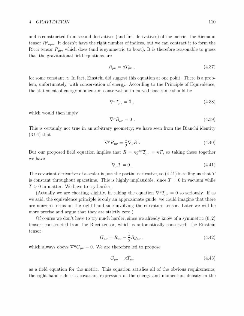
This is an equation relating derivatives of the metric to the energy density. To find the
explicit expression in terms of the metric, we need to evaluate R00 = Rλ0λ0. In fact we only
need Ri0i0, since R0
000 = 0. We have
Ri0j0 = ∂jΓ
i00 − ∂0Γ
ij0 + Γi
jλΓλ00 − Γi
0λΓλj0 . (4.49)
The second term here is a time derivative, which vanishes for static fields. The third and
fourth terms are of the form (Γ)2, and since Γ is first-order in the metric perturbation these
contribute only at second order, and can be neglected. We are left with Ri0j0 = ∂jΓ
i00. From
this we get
R00 = Ri0i0
= ∂i
(1
2giλ(∂0gλ0 + ∂0g0λ − ∂λg00)
)
= −1
2ηij∂i∂jh00
4 GRAVITATION 112
= −1
2∇2h00 . (4.50)
Comparing to (4.48), we see that the 00 component of (4.43) in the Newtonian limit predicts
∇2h00 = −κT00 . (4.51)
But this is exactly (4.36), if we set κ = 8πG.
So our guess seems to have worked out. With the normalization fixed by comparison
with the Newtonian limit, we can present Einstein’s equations for general relativity:
Rµν −1
2Rgµν = 8πGTµν . (4.52)
These tell us how the curvature of spacetime reacts to the presence of energy-momentum.
Einstein, you may have heard, thought that the left-hand side was nice and geometrical,
while the right-hand side was somewhat less compelling.
Einstein’s equations may be thought of as second-order differential equations for the
metric tensor field gµν . There are ten independent equations (since both sides are symmetric
two-index tensors), which seems to be exactly right for the ten unknown functions of the
metric components. However, the Bianchi identity ∇µGµν = 0 represents four constraints on
the functions Rµν , so there are only six truly independent equations in (4.52). In fact this is
appropriate, since if a metric is a solution to Einstein’s equation in one coordinate system
xµ it should also be a solution in any other coordinate system xµ′
. This means that there are
four unphysical degrees of freedom in gµν (represented by the four functions xµ′
(xµ)), and
we should expect that Einstein’s equations only constrain the six coordinate-independent
degrees of freedom.
As differential equations, these are extremely complicated; the Ricci scalar and tensor are
contractions of the Riemann tensor, which involves derivatives and products of the Christoffel
symbols, which in turn involve the inverse metric and derivatives of the metric. Furthermore,
the energy-momentum tensor Tµν will generally involve the metric as well. The equations
are also nonlinear, so that two known solutions cannot be superposed to find a third. It
is therefore very difficult to solve Einstein’s equations in any sort of generality, and it is
usually necessary to make some simplifying assumptions. Even in vacuum, where we set the
energy-momentum tensor to zero, the resulting equations (from (4.45))
Rµν = 0 (4.53)
can be very difficult to solve. The most popular sort of simplifying assumption is that the
metric has a significant degree of symmetry, and we will talk later on about how symmetries
of the metric make life easier.
The nonlinearity of general relativity is worth remarking on. In Newtonian gravity the
potential due to two point masses is simply the sum of the potentials for each mass, but
4 GRAVITATION 113
clearly this does not carry over to general relativity (outside the weak-field limit). There is
a physical reason for this, namely that in GR the gravitational field couples to itself. This
can be thought of as a consequence of the equivalence principle — if gravitation did not
couple to itself, a “gravitational atom” (two particles bound by their mutual gravitational
attraction) would have a different inertial mass (due to the negative binding energy) than
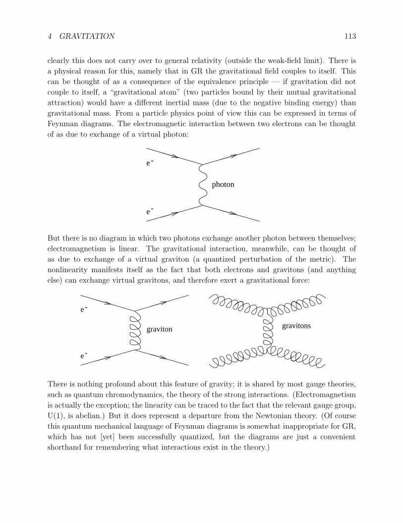
gravitational mass. From a particle physics point of view this can be expressed in terms of
Feynman diagrams. The electromagnetic interaction between two electrons can be thought
of as due to exchange of a virtual photon:
e
e-
-
photon
But there is no diagram in which two photons exchange another photon between themselves;
electromagnetism is linear. The gravitational interaction, meanwhile, can be thought of
as due to exchange of a virtual graviton (a quantized perturbation of the metric). The
nonlinearity manifests itself as the fact that both electrons and gravitons (and anything
else) can exchange virtual gravitons, and therefore exert a gravitational force:
e
e-
-
graviton gravitons
There is nothing profound about this feature of gravity; it is shared by most gauge theories,
such as quantum chromodynamics, the theory of the strong interactions. (Electromagnetism
is actually the exception; the linearity can be traced to the fact that the relevant gauge group,
U(1), is abelian.) But it does represent a departure from the Newtonian theory. (Of course
this quantum mechanical language of Feynman diagrams is somewhat inappropriate for GR,
which has not [yet] been successfully quantized, but the diagrams are just a convenient
shorthand for remembering what interactions exist in the theory.)
4 GRAVITATION 114
To increase your confidence that Einstein’s equations as we have derived them are indeed
the correct field equations for the metric, let’s see how they can be derived from a more
modern viewpoint, starting from an action principle. (In fact the equations were first derived
by Hilbert, not Einstein, and Hilbert did it using the action principle. But he had been
inspired by Einstein’s previous papers on the subject, and Einstein himself derived the
equations independently, so they are rightly named after Einstein. The action, however, is
rightly called the Hilbert action.) The action should be the integral over spacetime of a
Lagrange density (“Lagrangian” for short, although strictly speaking the Lagrangian is the
integral over space of the Lagrange density):
SH =∫dnxLH . (4.54)
The Lagrange density is a tensor density, which can be written as√−g times a scalar. What
scalars can we make out of the metric? Since we know that the metric can be set equal to
its canonical form and its first derivatives set to zero at any one point, any nontrivial scalar
must involve at least second derivatives of the metric. The Riemann tensor is of course
made from second derivatives of the metric, and we argued earlier that the only independent
scalar we could construct from the Riemann tensor was the Ricci scalar R. What we did not
show, but is nevertheless true, is that any nontrivial tensor made from the metric and its
first and second derivatives can be expressed in terms of the metric and the Riemann tensor.
Therefore, the only independent scalar constructed from the metric, which is no higher than
second order in its derivatives, is the Ricci scalar. Hilbert figured that this was therefore the
simplest possible choice for a Lagrangian, and proposed
LH =√−gR . (4.55)
The equations of motion should come from varying the action with respect to the metric.
In fact let us consider variations with respect to the inverse metric gµν , which are slightly
easier but give an equivalent set of equations. Using R = gµνRµν , in general we will have
δS =∫dnx
[√−ggµνδRµν +√−gRµνδg
µν +Rδ√−g
]
= (δS)1 + (δS)2 + (δS)3 . (4.56)
The second term (δS)2 is already in the form of some expression times δgµν ; let’s examine
the others more closely.
Recall that the Ricci tensor is the contraction of the Riemann tensor, which is given by
Rρµλν = ∂λΓ
λνµ + Γρ
λσΓσνµ − (λ↔ ν) . (4.57)
The variation of this with respect the metric can be found first varying the connection with
respect to the metric, and then substituting into this expression. Let us however consider
4 GRAVITATION 115
arbitrary variations of the connection, by replacing
Γρνµ → Γρ
νµ + δΓρνµ . (4.58)
The variation δΓρνµ is the difference of two connections, and therefore is itself a tensor. We
can thus take its covariant derivative,
∇λ(δΓρνµ) = ∂λ(δΓ
ρνµ) + Γρ
λσδΓσνµ − Γσ
λνδΓρσµ − Γσ
λµδΓρνσ . (4.59)
Given this expression (and a small amount of labor) it is easy to show that
δRρµλν = ∇λ(δΓ
ρνµ) −∇ν(δΓ
ρλµ) . (4.60)
You can check this yourself. Therefore, the contribution of the first term in (4.56) to δS can
be written
(δS)1 =∫dnx
√−g gµν[∇λ(δΓ
λνµ) −∇ν(δΓ
λλµ)]
=∫dnx
√−g ∇σ
[gµσ(δΓλ
λµ) − gµν(δΓσµν)], (4.61)
where we have used metric compatibility and relabeled some dummy indices. But now we
have the integral with respect to the natural volume element of the covariant divergence of
a vector; by Stokes’s theorem, this is equal to a boundary contribution at infinity which we
can set to zero by making the variation vanish at infinity. (We haven’t actually shown that
Stokes’s theorem, as mentioned earlier in terms of differential forms, can be thought of this
way, but you can easily convince yourself it’s true.) Therefore this term contributes nothing
to the total variation.
To make sense of the (δS)3 term we need to use the following fact, true for any matrix
M :
Tr(lnM) = ln(detM) . (4.62)
Here, lnM is defined by exp(lnM) = M . (For numbers this is obvious, for matrices it’s a
little less straightforward.) The variation of this identity yields
Tr(M−1δM) =1
detMδ(detM) . (4.63)
Here we have used the cyclic property of the trace to allow us to ignore the fact that M−1
and δM may not commute. Now we would like to apply this to the inverse metric, M = gµν .
Then detM = g−1 (where g = det gµν), and
δ(g−1) =1
ggµνδg
µν . (4.64)
4 GRAVITATION 116
Now we can just plug in:
δ√−g = δ[(−g−1)−1/2]
= −1
2(−g−1)−3/2δ(−g−1)
= −1
2
√−ggµνδgµν . (4.65)
Hearkening back to (4.56), and remembering that (δS)1 does not contribute, we find
δS =∫dnx
√−g[Rµν −
1
2Rgµν
]δgµν . (4.66)
This should vanish for arbitrary variations, so we are led to Einstein’s equations in vacuum:
1√−gδS
δgµν= Rµν −
1
2Rgµν = 0 . (4.67)
The fact that this simple action leads to the same vacuum field equations as we had
previously arrived at by more informal arguments certainly reassures us that we are doing
something right. What we would really like, however, is to get the non-vacuum field equations
as well. That means we consider an action of the form
S =1
8πGSH + SM , (4.68)
where SM is the action for matter, and we have presciently normalized the gravitational
action (although the proper normalization is somewhat convention-dependent). Following
through the same procedure as above leads to
1√−gδS
δgµν=
1
8πG
(Rµν −
1
2Rgµν
)+
1√−gδSM
δgµν= 0 , (4.69)
and we recover Einstein’s equations if we can set
Tµν = − 1√−gδSM
δgµν. (4.70)
What makes us think that we can make such an identification? In fact (4.70) turns out to
be the best way to define a symmetric energy-momentum tensor. The tricky part is to show
that it is conserved, which is in fact automatically true, but which we will not justify until
the next section.
We say that (4.70) provides the “best” definition of the energy-momentum tensor because
it is not the only one you will find. In flat Minkowski space, there is an alternative defini-
tion which is sometimes given in books on electromagnetism or field theory. In this context
4 GRAVITATION 117
energy-momentum conservation arises as a consequence of symmetry of the Lagrangian un-
der spacetime translations. Noether’s theorem states that every symmetry of a Lagrangian
implies the existence of a conservation law; invariance under the four spacetime translations
leads to a tensor Sµν which obeys ∂µSµν = 0 (four relations, one for each value of ν). The
details can be found in Wald or in any number of field theory books. Applying Noether’s
procedure to a Lagrangian which depends on some fields ψi and their first derivatives ∂µψi,
we obtain
Sµν =δL
δ(∂µψi)∂νψi − ηµνL , (4.71)
where a sum over i is implied. You can check that this tensor is conserved by virtue of the
equations of motion of the matter fields. Sµν often goes by the name “canonical energy-
momentum tensor”; however, there are a number of reasons why it is more convenient for
us to use (4.70). First and foremost, (4.70) is in fact what appears on the right hand side of
Einstein’s equations when they are derived from an action, and it is not always possible to
generalize (4.71) to curved spacetime. But even in flat space (4.70) has its advantages; it is
manifestly symmetric, and also guaranteed to be gauge invariant, neither of which is true for
(4.71). We will therefore stick with (4.70) as the definition of the energy-momentum tensor.
Sometimes it is useful to think about Einstein’s equations without specifying the theory
of matter from which Tµν is derived. This leaves us with a great deal of arbitrariness; consider
for example the question “What metrics obey Einstein’s equations?” In the absence of some
constraints on Tµν , the answer is “any metric at all”; simply take the metric of your choice,
compute the Einstein tensor Gµν for this metric, and then demand that Tµν be equal to Gµν .
(It will automatically be conserved, by the Bianchi identity.) Our real concern is with the
existence of solutions to Einstein’s equations in the presence of “realistic” sources of energy
and momentum, whatever that means. The most common property that is demanded of
Tµν is that it represent positive energy densities — no negative masses are allowed. In a
locally inertial frame this requirement can be stated as ρ = T00 ≥ 0. To turn this into a
coordinate-independent statement, we ask that
TµνVµV ν ≥ 0 , for all timelike vectors V µ . (4.72)
This is known as the Weak Energy Condition, or WEC. It seems like a fairly reasonable
requirement, and many of the important theorems about solutions to general relativity (such
as the singularity theorems of Hawking and Penrose) rely on this condition or something
very close to it. Unfortunately it is not set in stone; indeed, it is straightforward to invent
otherwise respectable classical field theories which violate the WEC, and almost impossible
to invent a quantum field theory which obeys it. Nevertheless, it is legitimate to assume
that the WEC holds in all but the most extreme conditions. (There are also stronger energy
conditions, but they are even less true than the WEC, and we won’t dwell on them.)
4 GRAVITATION 118
We have now justified Einstein’s equations in two different ways: as the natural covariant
generalization of Poisson’s equation for the Newtonian gravitational potential, and as the
result of varying the simplest possible action we could invent for the metric. The rest of
the course will be an exploration of the consequences of these equations, but before we start
on that road let us briefly explore ways in which the equations could be modified. There
are an uncountable number of such ways, but we will consider four different possibilities:
the introduction of a cosmological constant, higher-order terms in the action, gravitational
scalar fields, and a nonvanishing torsion tensor.
The first possibility is the cosmological constant; George Gamow has quoted Einstein as
calling this the biggest mistake of his life. Recall that in our search for the simplest possible
action for gravity we noted that any nontrivial scalar had to be of at least second order in
derivatives of the metric; at lower order all we can create is a constant. Although a constant
does not by itself lead to very interesting dynamics, it has an important effect if we add it
to the conventional Hilbert action. We therefore consider an action given by
S =∫dnx
√−g(R− 2Λ) , (4.73)
where Λ is some constant. The resulting field equations are
Rµν −1
2Rgµν + Λgµν = 0 , (4.74)
and of course there would be an energy-momentum tensor on the right hand side if we had
included an action for matter. Λ is the cosmological constant; it was originally introduced
by Einstein after it became clear that there were no solutions to his equations representing
a static cosmology (a universe unchanging with time on large scales) with a nonzero matter
content. If the cosmological constant is tuned just right, it is possible to find a static solution,
but it is unstable to small perturbations. Furthermore, once Hubble demonstrated that the
universe is expanding, it became less important to find static solutions, and Einstein rejected
his suggestion. Like Rasputin, however, the cosmological constant has proven difficult to kill
off. If we like we can move the additional term in (4.74) to the right hand side, and think of
it as a kind of energy-momentum tensor, with Tµν = −Λgµν (it is automatically conserved
by metric compatibility). Then Λ can be interpreted as the “energy density of the vacuum,”
a source of energy and momentum that is present even in the absence of matter fields. This
interpretation is important because quantum field theory predicts that the vacuum should
have some sort of energy and momentum. In ordinary quantum mechanics, an harmonic
oscillator with frequency ω and minimum classical energy E0 = 0 upon quantization has a
ground state with energy E0 = 12hω. A quantized field can be thought of as a collection of
an infinite number of harmonic oscillators, and each mode contributes to the ground state
energy. The result is of course infinite, and must be appropriately regularized, for example
4 GRAVITATION 119
by introducing a cutoff at high frequencies. The final vacuum energy, which is the regularized
sum of the energies of the ground state oscillations of all the fields of the theory, has no good
reason to be zero and in fact would be expected to have a natural scale
Λ ∼ m4P , (4.75)
where the Planck mass mP is approximately 1019 GeV, or 10−5 grams. Observations of the
universe on large scales allow us to constrain the actual value of Λ, which turns out to be
smaller than (4.75) by at least a factor of 10120. This is the largest known discrepancy between
theoretical estimate and observational constraint in physics, and convinces many people that
the “cosmological constant problem” is one of the most important unsolved problems today.
On the other hand the observations do not tell us that Λ is strictly zero, and in fact allow
values that can have important consequences for the evolution of the universe. This mistake
of Einstein’s therefore continues to bedevil both physicists, who would like to understand
why it is so small, and astronomers, who would like to determine whether it is really small
enough to be ignored.
A somewhat less intriguing generalization of the Hilbert action would be to include scalars
of more than second order in derivatives of the metric. We could imagine an action of the
form
S =∫dnx
√−g(R + α1R2 + α2RµνR
µν + α3gµν∇µR∇νR + · · ·) , (4.76)
where the α’s are coupling constants and the dots represent every other scalar we can make
from the curvature tensor, its contractions, and its derivatives. Traditionally, such terms
have been neglected on the reasonable grounds that they merely complicate a theory which
is already both aesthetically pleasing and empirically successful. However, there are at
least three more substantive reasons for this neglect. First, as we shall see below, Einstein’s
equations lead to a well-posed initial value problem for the metric, in which “coordinates” and
“momenta” specified at an initial time can be used to predict future evolution. With higher-
derivative terms, we would require not only those data, but also some number of derivatives
of the momenta. Second, the main source of dissatisfaction with general relativity on the part
of particle physicists is that it cannot be renormalized (as far as we know), and Lagrangians
with higher derivatives tend generally to make theories less renormalizable rather than more.
Third, by the same arguments we used above when speaking about the limitations of the
principle of equivalence, the extra terms in (4.76) should be suppressed (by powers of the
Planck mass to some power) relative to the usual Hilbert term, and therefore would not be
expected to be of any practical importance to the low-energy world. None of these reasons
are completely persuasive, and indeed people continue to consider such theories, but for the
most part these models do not attract a great deal of attention.
A set of models which does attract attention are known as scalar-tensor theories of
gravity, since they involve both the metric tensor gµν and a fundamental scalar field, λ. The
4 GRAVITATION 120
action can be written
S =∫dnx
√−g[f(λ)R+
1
2gµν(∂µλ)(∂νλ) − V (λ)
], (4.77)
where f(λ) and V (λ) are functions which define the theory. Recall from (4.68) that the
coefficient of the Ricci scalar in conventional GR is proportional to the inverse of Newton’s
constant G. In scalar-tensor theories, then, where this coefficient is replaced by some function
of a field which can vary throughout spacetime, the “strength” of gravity (as measured by
the local value of Newton’s constant) will be different from place to place and time to time.
In fact the most famous scalar-tensor theory, invented by Brans and Dicke and now named
after them, was inspired by a suggestion of Dirac’s that the gravitational constant varies
with time. Dirac had noticed that there were some interesting numerical coincidences one
could discover by taking combinations of cosmological numbers such as the Hubble constant
H0 (a measure of the expansion rate of the universe) and typical particle-physics parameters
such as the mass of the pion, mπ. For example,
m3π
H0
∼ cG
h2 . (4.78)
If we assume for the moment that this relation is not simply an accident, we are faced with
the problem that the Hubble “constant” actually changes with time (in most cosmological
models), while the other quantities conventionally do not. Dirac therefore proposed that in
fact G varied with time, in such a way as to maintain (4.78); satisfying this proposal was
the motivation of Brans and Dicke. These days, experimental test of general relativity are
sufficiently precise that we can state with confidence that, if Brans-Dicke theory is correct,
the predicted change in G over space and time must be very small, much slower than that
necessary to satisfy Dirac’s hypothesis. (See Weinberg for details on Brans-Dicke theory
and experimental tests.) Nevertheless there is still a great deal of work being done on other
kinds of scalar-tensor theories, which turn out to be vital in superstring theory and may
have important consequences in the very early universe.
As a final alternative to general relativity, we should mention the possibility that the
connection really is not derived from the metric, but in fact has an independent existence as a
fundamental field. We will leave it as an exercise for you to show that it is possible to consider
the conventional action for general relativity but treat it as a function of both the metric
gµν and a torsion-free connection Γλρσ, and the equations of motion derived from varying
such an action with respect to the connection imply that Γλρσ is actually the Christoffel
connection associated with gµν . We could drop the demand that the connection be torsion-
free, in which case the torsion tensor could lead to additional propagating degrees of freedom.
Without going into details, the basic reason why such theories do not receive much attention
is simply because the torsion is itself a tensor; there is nothing to distinguish it from other,
4 GRAVITATION 121
“non-gravitational” tensor fields. Thus, we do not really lose any generality by considering
theories of torsion-free connections (which lead to GR) plus any number of tensor fields,
which we can name what we like.
With the possibility in mind that one of these alternatives (or, more likely, something
we have not yet thought of) is actually realized in nature, for the rest of the course we will
work under the assumption that general relativity as based on Einstein’s equations or the
Hilbert action is the correct theory, and work out its consequences. These consequences, of
course, are constituted by the solutions to Einstein’s equations for various sources of energy
and momentum, and the behavior of test particles in these solutions. Before considering
specific solutions in detail, lets look more abstractly at the initial-value problem in general
relativity.
In classical Newtonian mechanics, the behavior of a single particle is of course governed
by f = ma. If the particle is moving under the influence of some potential energy field Φ(x),
then the force is f = −∇Φ, and the particle obeys
md2xi
dt2= −∂iΦ . (4.79)
This is a second-order differential equation for xi(t), which we can recast as a system of two
coupled first-order equations by introducing the momentum p:
dpi
dt= −∂iΦ
dxi
dt=
1
mpi . (4.80)
The initial-value problem is simply the procedure of specifying a “state” (xi, pi) which serves
as a boundary condition with which (4.80) can be uniquely solved. You may think of (4.80)
as allowing you, once you are given the coordinates and momenta at some time t, to evolve
them forward an infinitesimal amount to a time t+ δt, and iterate this procedure to obtain
the entire solution.
We would like to formulate the analogous problem in general relativity. Einstein’s equa-
tions Gµν = 8πGTµν are of course covariant; they don’t single out a preferred notion of “time”
through which a state can evolve. Nevertheless, we can by hand pick a spacelike hypersurface
(or “slice”) Σ, specify initial data on that hypersurface, and see if we can evolve uniquely
from it to a hypersurface in the future. (“Hyper” because a constant-time slice in four di-
mensions will be three-dimensional, whereas “surfaces” are conventionally two-dimensional.)
This process does violence to the manifest covariance of the theory, but if we are careful we
should wind up with a formulation that is equivalent to solving Einstein’s equations all at
once throughout spacetime.
Since the metric is the fundamental variable, our first guess is that we should consider
the values gµν |Σ of the metric on our hypersurface to be the “coordinates” and the time
4 GRAVITATION 122
Initial DataΣ
t
derivatives ∂tgµν |Σ (with respect to some specified time coordinate) to be the “momenta”,
which together specify the state. (There will also be coordinates and momenta for the matter
fields, which we will not consider explicitly.) In fact the equations Gµν = 8πGTµν do involve
second derivatives of the metric with respect to time (since the connection involves first
derivatives of the metric and the Einstein tensor involves first derivatives of the connection),
so we seem to be on the right track. However, the Bianchi identity tells us that ∇µGµν = 0.
We can rewrite this equation as
∂0G0ν = −∂iG
iν − ΓµµλG
λν − ΓνµλG
µλ . (4.81)
A close look at the right hand side reveals that there are no third-order time derivatives;
therefore there cannot be any on the left hand side. Thus, although Gµν as a whole involves
second-order time derivatives of the metric, the specific components G0ν do not. Of the ten
independent components in Einstein’s equations, the four represented by
G0ν = 8πGT 0ν (4.82)
cannot be used to evolve the initial data (gµν , ∂tgµν)Σ. Rather, they serve as constraints
on this initial data; we are not free to specify any combination of the metric and its time
derivatives on the hypersurface Σ, since they must obey the relations (4.82). The remaining
equations,
Gij = 8πGT ij (4.83)
are the dynamical evolution equations for the metric. Of course, these are only six equations
for the ten unknown functions gµν(xσ), so the solution will inevitably involve a fourfold
ambiguity. This is simply the freedom that we have already mentioned, to choose the four
coordinate functions throughout spacetime.
It is a straightforward but unenlightening exercise to sift through (4.83) to find that
not all second time derivatives of the metric appear. In fact we find that ∂2t gij appears in
(4.83), but not ∂2t g0ν . Therefore a “state” in general relativity will consist of a specification
4 GRAVITATION 123
of the spacelike components of the metric gij|Σ and their first time derivatives ∂tgij|Σ on the
hypersurface Σ, from which we can determine the future evolution using (4.83), up to an
unavoidable ambiguity in fixing the remaining components g0ν . The situation is precisely
analogous to that in electromagnetism, where we know that no amount of initial data can
suffice to determine the evolution uniquely since there will always be the freedom to perform a
gauge transformation Aµ → Aµ+∂µλ. In general relativity, then, coordinate transformations
play a role reminiscent of gauge transformations in electromagnetism, in that they introduce
ambiguity into the time evolution.
One way to cope with this problem is to simply “choose a gauge.” In electromagnetism
this means to place a condition on the vector potential Aµ, which will restrict our freedom
to perform gauge transformations. For example we can choose Lorentz gauge, in which
∇µAµ = 0, or temporal gauge, in which A0 = 0. We can do a similar thing in general
relativity, by fixing our coordinate system. A popular choice is harmonic gauge (also
known as Lorentz gauge and a host of other names), in which
2xµ = 0 . (4.84)
Here 2 = ∇µ∇µ is the covariant D’Alembertian, and it is crucial to realize when we take
the covariant derivative that the four functions xµ are just functions, not components of a
vector. This condition is therefore simply
0 = 2xµ
= gρσ∂ρ∂σxµ − gρσΓλ
ρσ∂λxµ
= −gρσΓλρσ . (4.85)
In flat space, of course, Cartesian coordinates (in which Γλρσ = 0) are harmonic coordi-
nates. (As a general principle, any function f which satisfies 2f = 0 is called an “harmonic
function.”)
To see that this choice of coordinates successfully fixes our gauge freedom, let’s rewrite
the condition (4.84) in a somewhat simpler form. We have
gρσΓµρσ =
1
2gρσgµν(∂ρgσν + ∂σgνρ − ∂νgρσ) , (4.86)
from the definition of the Christoffel symbols. Meanwhile, from ∂ρ(gµνgσν) = ∂ρδ
µσ = 0 we
have
gµν∂ρgσν = −gσν∂ρgµν . (4.87)
Also, from our previous exploration of the variation of the determinant of the metric (4.65),
we have1
2gρσ∂νg
ρσ = − 1√−g ∂ν
√−g . (4.88)
4 GRAVITATION 124
Putting it all together, we find that (in general),
gρσΓµρσ =
1√−g ∂λ(√−ggλµ) . (4.89)
The harmonic gauge condition (4.85) therefore is equivalent to
∂λ(√−ggλµ) = 0 . (4.90)
Taking the partial derivative of this with respect to t = x0 yields
∂2
∂t2(√−gg0ν) = − ∂
∂xi
[∂
∂t(√−ggiν)
]. (4.91)
This condition represents a second-order differential equation for the previously uncon-
strained metric components g0ν , in terms of the given initial data. We have therefore
succeeded in fixing our gauge freedom, in that we can now solve for the evolution of the
entire metric in harmonic coordinates. (At least locally; we have been glossing over the fact
our gauge choice may not be well-defined globally, and we would have to resort to working
in patches as usual. The same problem appears in gauge theories in particle physics.) Note
that we still have some freedom remaining; our gauge condition (4.84) restricts how the
coordinates stretch from our initial hypersurface Σ throughout spacetime, but we can still
choose coordinates xi on Σ however we like. This corresponds to the fact that making a
coordinate transformation xµ → xµ + δµ, with 2δµ = 0, does not violate the harmonic gauge
condition.
We therefore have a well-defined initial value problem for general relativity; a state is
specified by the spacelike components of the metric and their time derivatives on a spacelike
hypersurface Σ; given these, the spacelike components (4.83) of Einstein’s equations allow
us to evolve the metric forward in time, up to an ambiguity in coordinate choice which
may be resolved by choice of gauge. We must keep in mind that the initial data are not
arbitrary, but must obey the constraints (4.82). (Once we impose the constraints on some
spacelike hypersurface, the equations of motion guarantee that they remain satisfied, as you
can check.) The constraints serve a useful purpose, of guaranteeing that the result remains
spacetime covariant after we have split our manifold into “space” and “time.” Specifically,
the Gi0 = 8πGT i0 constraint implies that the evolution is independent of our choice of
coordinates on Σ, while G00 = 8πGT 00 enforces invariance under different ways of slicing
spacetime into spacelike hypersurfaces.
Once we have seen how to cast Einstein’s equations as an initial value problem, one issue
of crucial importance is the existence of solutions to the problem. That is, once we have
specified a spacelike hypersurface with initial data, to what extent can we be guaranteed
that a unique spacetime will be determined? Although one can do a great deal of hard work
4 GRAVITATION 125
Σ
to answer this question with some precision, it is fairly simple to get a handle on the ways
in which a well-defined solution can fail to exist, which we now consider.
It is simplest to first consider the problem of evolving matter fields on a fixed background
spacetime, rather than the evolution of the metric itself. We therefore consider a spacelike
hypersurface Σ in some manifold M with fixed metric gµν , and furthermore look at some
connected subset S in Σ. Our guiding principle will be that no signals can travel faster than
the speed of light; therefore “information” will only flow along timelike or null trajectories
(not necessarily geodesics). We define the future domain of dependence of S, denoted
D+(S), as the set of all points p such that every past-moving, timelike or null, inextendible
curve through p must intersect S. (“Inextendible” just means that the curve goes on forever,
not ending at some finite point.) We interpret this definition in such a way that S itself is a
subset of D+(S). (Of course a rigorous formulation does not require additional interpretation
over and above the definitions, but we are not being as rigorous as we could be right now.)
Similarly, we define the past domain of dependence D−(S) in the same way, but with “past-
moving” replaced by “future-moving.” Generally speaking, some points in M will be in one
of the domains of dependence, and some will be outside; we define the boundary of D+(S)
to be the future Cauchy horizon H+(S), and likewise the boundary of D−(S) to be the
past Cauchy horizon H−(S). You can convince yourself that they are both null surfaces.
Σ S
D (S)
H (S) D (S)
H (S)+
- -
+
4 GRAVITATION 126
The usefulness of these definitions should be apparent; if nothing moves faster than light,
than signals cannot propagate outside the light cone of any point p. Therefore, if every
curve which remains inside this light cone must intersect S, then information specified on S
should be sufficient to predict what the situation is at p. (That is, initial data for matter
fields given on S can be used to solve for the value of the fields at p.) The set of all points
for which we can predict what happens by knowing what happens on S is simply the union
D+(S) ∪D−(S).
We can easily extend these ideas from the subset S to the entire hypersurface Σ. The
important point is that D+(Σ) ∪D−(Σ) might fail to be all of M , even if Σ itself seems like
a perfectly respectable hypersurface that extends throughout space. There are a number
of ways in which this can happen. One possibility is that we have just chosen a “bad”
hypersurface (although it is hard to give a general prescription for when a hypersurface is
bad in this sense). Consider Minkowski space, and a spacelike hypersurface Σ which remains
to the past of the light cone of some point.
Σ
D ( )Σ+
In this case Σ is a nice spacelike surface, but it is clear that D+(Σ) ends at the light cone,
and we cannot use information on Σ to predict what happens throughout Minkowski space.
Of course, there are other surfaces we could have picked for which the domain of dependence
would have been the entire manifold, so this doesn’t worry us too much.
A somewhat more nontrivial example is known as Misner space. This is a two-
dimensional spacetime with the topology of R1 × S1, and a metric for which the light cones
progressively tilt as you go forward in time. Past a certain point, it is possible to travel on a
timelike trajectory which wraps around the S1 and comes back to itself; this is known as a
closed timelike curve. If we had specified a surface Σ to this past of this point, then none
of the points in the region containing closed timelike curves are in the domain of dependence
of Σ, since the closed timelike curves themselves do not intersect Σ. This is obviously a worse
problem than the previous one, since a well-defined initial value problem does not seem to
4 GRAVITATION 127
Σ
identify
closedtimelikecurve
Misnerspace
exist in this spacetime. (Actually problems like this are the subject of some current research
interest, so I won’t claim that the issue is settled.)
A final example is provided by the existence of singularities, points which are not in the
manifold even though they can be reached by travelling along a geodesic for a finite distance.
Typically these occur when the curvature becomes infinite at some point; if this happens,
the point can no longer be said to be part of the spacetime. Such an occurrence can lead to
the emergence of a Cauchy horizon — a point p which is in the future of a singularity cannot
be in the domain of dependence of a hypersurface to the past of the singularity, because
there will be curves from p which simply end at the singularity.
Σ
Σ
D ( )
H ( )
Σ+
+
All of these obstacles can also arise in the initial value problem for GR, when we try to
evolve the metric itself from initial data. However, they are of different degrees of trouble-
4 GRAVITATION 128
someness. The possibility of picking a “bad” initial hypersurface does not arise very often,
especially since most solutions are found globally (by solving Einstein’s equations throughout
spacetime). The one situation in which you have to be careful is in numerical solution of Ein-
stein’s equations, where a bad choice of hypersurface can lead to numerical difficulties even
if in principle a complete solution exists. Closed timelike curves seem to be something that
GR works hard to avoid — there are certainly solutions which contain them, but evolution
from generic initial data does not usually produce them. Singularities, on the other hand,
are practically unavoidable. The simple fact that the gravitational force is always attractive
tends to pull matter together, increasing the curvature, and generally leading to some sort of
singularity. This is something which we apparently must learn to live with, although there
is some hope that a well-defined theory of quantum gravity will eliminate the singularities
of classical GR.
December 1997 Lecture Notes on General Relativity Sean M. Carroll
5 More Geometry
With an understanding of how the laws of physics adapt to curved spacetime, it is undeniably
tempting to start in on applications. However, a few extra mathematical techniques will
simplify our task a great deal, so we will pause briefly to explore the geometry of manifolds
some more.
When we discussed manifolds in section 2, we introduced maps between two different
manifolds and how maps could be composed. We now turn to the use of such maps in carrying
along tensor fields from one manifold to another. We therefore consider two manifolds M
and N , possibly of different dimension, with coordinate systems xµ and yα, respectively. We
imagine that we have a map φ : M → N and a function f : N → R.
M
x
f = f
fφ
R
R
Rm n
µ yα
N
*φ φ
It is obvious that we can compose φ with f to construct a map (f φ) : M → R, which is
simply a function on M . Such a construction is sufficiently useful that it gets its own name;
we define the pullback of f by φ, denoted φ∗f , by
φ∗f = (f φ) . (5.1)
The name makes sense, since we think of φ∗ as “pulling back” the function f from N to M .
We can pull functions back, but we cannot push them forward. If we have a function
g : M → R, there is no way we can compose g with φ to create a function on N ; the arrows
don’t fit together correctly. But recall that a vector can be thought of as a derivative operator
that maps smooth functions to real numbers. This allows us to define the pushforward of
129
5 MORE GEOMETRY 130
a vector; if V (p) is a vector at a point p on M , we define the pushforward vector φ∗V at the
point φ(p) on N by giving its action on functions on N :
(φ∗V )(f) = V (φ∗f) . (5.2)
So to push forward a vector field we say “the action of φ∗V on any function is simply the
action of V on the pullback of that function.”
This is a little abstract, and it would be nice to have a more concrete description. We
know that a basis for vectors on M is given by the set of partial derivatives ∂µ = ∂∂xµ , and
a basis on N is given by the set of partial derivatives ∂α = ∂∂yα . Therefore we would like
to relate the components of V = V µ∂µ to those of (φ∗V ) = (φ∗V )α∂α. We can find the
sought-after relation by applying the pushed-forward vector to a test function and using the
chain rule (2.3):
(φ∗V )α∂αf = V µ∂µ(φ∗f)
= V µ∂µ(f φ)
= V µ∂yα
∂xµ∂αf . (5.3)
This simple formula makes it irresistible to think of the pushforward operation φ∗ as a matrix
operator, (φ∗V )α = (φ∗)αµV
µ, with the matrix being given by
(φ∗)αµ =
∂yα
∂xµ. (5.4)
The behavior of a vector under a pushforward thus bears an unmistakable resemblance to the
vector transformation law under change of coordinates. In fact it is a generalization, since
when M and N are the same manifold the constructions are (as we shall discuss) identical;
but don’t be fooled, since in general µ and α have different allowed values, and there is no
reason for the matrix ∂yα/∂xµ to be invertible.
It is a rewarding exercise to convince yourself that, although you can push vectors forward
from M to N (given a map φ : M → N), you cannot in general pull them back — just keep
trying to invent an appropriate construction until the futility of the attempt becomes clear.
Since one-forms are dual to vectors, you should not be surprised to hear that one-forms can
be pulled back (but not in general pushed forward). To do this, remember that one-forms
are linear maps from vectors to the real numbers. The pullback φ∗ω of a one-form ω on N
can therefore be defined by its action on a vector V on M , by equating it with the action of
ω itself on the pushforward of V :
(φ∗ω)(V ) = ω(φ∗V ) . (5.5)
Once again, there is a simple matrix description of the pullback operator on forms, (φ∗ω)µ =
(φ∗)µαωα, which we can derive using the chain rule. It is given by
(φ∗)µα =
∂yα
∂xµ. (5.6)
5 MORE GEOMETRY 131
That is, it is the same matrix as the pushforward (5.4), but of course a different index is
contracted when the matrix acts to pull back one-forms.
There is a way of thinking about why pullbacks and pushforwards work on some objects
but not others, which may or may not be helpful. If we denote the set of smooth functions
on M by F(M), then a vector V (p) at a point p on M (i.e., an element of the tangent space
TpM) can be thought of as an operator from F(M) to R. But we already know that the
pullback operator on functions maps F(N) to F(M) (just as φ itself maps M to N , but
in the opposite direction). Therefore we can define the pushforward φ∗ acting on vectors
simply by composing maps, as we first defined the pullback of functions:
F F(M) (N)
φ*(V(p)) = V(p) φ
R
φ
V(p)*
*
Similarly, if TqN is the tangent space at a point q on N , then a one-form ω at q (i.e., an
element of the cotangent space T ∗q N) can be thought of as an operator from TqN to R. Since
the pushforward φ∗ maps TpM to Tφ(p)N , the pullback φ∗ of a one-form can also be thought
of as mere composition of maps:
T Mp φ(p)T N
φ*= ω(ω)*
φ
φ*
ω
R
If this is not helpful, don’t worry about it. But do keep straight what exists and what
doesn’t; the actual concepts are simple, it’s just remembering which map goes what way
that leads to confusion.
You will recall further that a (0, l) tensor — one with l lower indices and no upper ones
— is a linear map from the direct product of l vectors to R. We can therefore pull back
not only one-forms, but tensors with an arbitrary number of lower indices. The definition is
simply the action of the original tensor on the pushed-forward vectors:
(φ∗T )(V (1), V (2), . . . , V (l)) = T (φ∗V (1), φ∗V (2), . . . , φ∗V (l)) , (5.7)
5 MORE GEOMETRY 132
where Tα1···αlis a (0, l) tensor on N . We can similarly push forward any (k, 0) tensor Sµ1···µk
by acting it on pulled-back one-forms:
(φ∗S)(ω(1), ω(2), . . . , ω(k)) = S(φ∗ω(1), φ∗ω
(2), . . . , φ∗ω(k)) . (5.8)
Fortunately, the matrix representations of the pushforward (5.4) and pullback (5.6) extend to
the higher-rank tensors simply by assigning one matrix to each index; thus, for the pullback
of a (0, l) tensor, we have
(φ∗T )µ1···µl=∂yα1
∂xµ1· · · ∂y
αl
∂xµlTα1···αl
, (5.9)
while for the pushforward of a (k, 0) tensor we have
(φ∗S)α1···αk =∂yα1
∂xµ1· · · ∂y
αk
∂xµkSµ1···µk . (5.10)
Our complete picture is therefore:
φ*
φ*( )
( )k0 ( )k
0
l l0 ( )0
φNM
Note that tensors with both upper and lower indices can generally be neither pushed forward
nor pulled back.
This machinery becomes somewhat less imposing once we see it at work in a simple
example. One common occurrence of a map between two manifolds is when M is actually a
submanifold of N ; then there is an obvious map from M to N which just takes an element
of M to the “same” element of N . Consider our usual example, the two-sphere embedded in
R3, as the locus of points a unit distance from the origin. If we put coordinates xµ = (θ, φ)
on M = S2 and yα = (x, y, z) on N = R3, the map φ : M → N is given by
φ(θ, φ) = (sin θ cos φ, sin θ sin φ, cos θ) . (5.11)
In the past we have considered the metric ds2 = dx2 + dy2 + dz2 on R3, and said that it
induces a metric dθ2 + sin2 θ dφ2 on S2, just by substituting (5.11) into this flat metric on
5 MORE GEOMETRY 133
R3. We didn’t really justify such a statement at the time, but now we can do so. (Of course
it would be easier if we worked in spherical coordinates on R3, but doing it the hard way is
more illustrative.) The matrix of partial derivatives is given by
∂yα
∂xµ=(
cos θ cosφ cos θ sin φ − sin θ− sin θ sinφ sin θ cos φ 0
). (5.12)
The metric on S2 is obtained by simply pulling back the metric from R3,
(φ∗g)µν =∂yα
∂xµ
∂yβ
∂xνgαβ
=(
1 00 sin2 θ
), (5.13)
as you can easily check. Once again, the answer is the same as you would get by naive
substitution, but now we know why.
We have been careful to emphasize that a map φ : M → N can be used to push certain
things forward and pull other things back. The reason why it generally doesn’t work both
ways can be traced to the fact that φ might not be invertible. If φ is invertible (and both φ
and φ−1 are smooth, which we always implicitly assume), then it defines a diffeomorphism
between M and N . In this case M and N are the same abstract manifold. The beauty of
diffeomorphisms is that we can use both φ and φ−1 to move tensors from M to N ; this will
allow us to define the pushforward and pullback of arbitrary tensors. Specifically, for a (k, l)
tensor field T µ1···µkν1···µl
on M , we define the pushforward by
(φ∗T )(ω(1), . . . , ω(k), V (1), . . . , V (l)) = T (φ∗ω(1), . . . , φ∗ω
(k), [φ−1]∗V (1), . . . , [φ−1]∗V (l)) ,
(5.14)
where the ω(i)’s are one-forms on N and the V (i)’s are vectors on N . In components this
becomes
(φ∗T )α1···αkβ1···βl
=∂yα1
∂xµ1· · · ∂y
αk
∂xµk
∂xν1
∂yβ1· · · ∂x
νl
∂yβlT µ1···µk
ν1···νl. (5.15)
The appearance of the inverse matrix ∂xν/∂yβ is legitimate because φ is invertible. Note
that we could also define the pullback in the obvious way, but there is no need to write
separate equations because the pullback φ∗ is the same as the pushforward via the inverse
map, [φ−1]∗.
We are now in a position to explain the relationship between diffeomorphisms and coordi-
nate transformations. The relationship is that they are two different ways of doing precisely
the same thing. If you like, diffeomorphisms are “active coordinate transformations”, while
traditional coordinate transformations are “passive.” Consider an n-dimensional manifold
M with coordinate functions xµ : M → Rn. To change coordinates we can either simply
introduce new functions yµ : M → Rn (“keep the manifold fixed, change the coordinate
5 MORE GEOMETRY 134
maps”), or we could just as well introduce a diffeomorphism φ : M → M , after which the
coordinates would just be the pullbacks (φ∗x)µ : M → Rn (“move the points on the man-
ifold, and then evaluate the coordinates of the new points”). In this sense, (5.15) really is
the tensor transformation law, just thought of from a different point of view.
φ*
φ
n
( x)
x
y
µ
µ
µ
R
M
Since a diffeomorphism allows us to pull back and push forward arbitrary tensors, it
provides another way of comparing tensors at different points on a manifold. Given a diffeo-
morphism φ : M →M and a tensor field T µ1···µkν1···µl
(x), we can form the difference between
the value of the tensor at some point p and φ∗[Tµ1···µk
ν1···µl(φ(p))], its value at φ(p) pulled
back to p. This suggests that we could define another kind of derivative operator on tensor
fields, one which categorizes the rate of change of the tensor as it changes under the diffeo-
morphism. For that, however, a single discrete diffeomorphism is insufficient; we require a
one-parameter family of diffeomorphisms, φt. This family can be thought of as a smooth
map R×M →M , such that for each t ∈ R φt is a diffeomorphism and φs φt = φs+t. Note
that this last condition implies that φ0 is the identity map.
One-parameter families of diffeomorphisms can be thought of as arising from vector fields
(and vice-versa). If we consider what happens to the point p under the entire family φt, it is
clear that it describes a curve in M ; since the same thing will be true of every point on M ,
these curves fill the manifold (although there can be degeneracies where the diffeomorphisms
have fixed points). We can define a vector field V µ(x) to be the set of tangent vectors to
each of these curves at every point, evaluated at t = 0. An example on S2 is provided by
the diffeomorphism φt(θ, φ) = (θ, φ+ t).
We can reverse the construction to define a one-parameter family of diffeomorphisms
from any vector field. Given a vector field V µ(x), we define the integral curves of the
vector field to be those curves xµ(t) which solve
dxµ
dt= V µ . (5.16)
Note that this familiar-looking equation is now to be interpreted in the opposite sense from
our usual way — we are given the vectors, from which we define the curves. Solutions to
5 MORE GEOMETRY 135
φ
(5.16) are guaranteed to exist as long as we don’t do anything silly like run into the edge of
our manifold; any standard differential geometry text will have the proof, which amounts to
finding a clever coordinate system in which the problem reduces to the fundamental theorem
of ordinary differential equations. Our diffeomorphisms φt represent “flow down the integral
curves,” and the associated vector field is referred to as the generator of the diffeomorphism.
(Integral curves are used all the time in elementary physics, just not given the name. The
“lines of magnetic flux” traced out by iron filings in the presence of a magnet are simply the
integral curves of the magnetic field vector B.)
Given a vector field V µ(x), then, we have a family of diffeomorphisms parameterized by
t, and we can ask how fast a tensor changes as we travel down the integral curves. For each
t we can define this change as
∆tTµ1···µk
ν1···µl(p) = φt∗[T
µ1···µkν1···µl
(φt(p))] − T µ1···µkν1···µl
(p) . (5.17)
Note that both terms on the right hand side are tensors at p.
T[ (p)]φt
(p)
p
[T( (p))]φt tφ*
T(p)
x (t)µ
φt
M
We then define the Lie derivative of the tensor along the vector field as
£V T µ1 ···µkν1 ···µl
= limt→0
(∆tT
µ1 ···µkν1 ···µl
t
). (5.18)
5 MORE GEOMETRY 136
The Lie derivative is a map from (k, l) tensor fields to (k, l) tensor fields, which is manifestly
independent of coordinates. Since the definition essentially amounts to the conventional
definition of an ordinary derivative applied to the component functions of the tensor, it
should be clear that it is linear,
£V (aT + bS ) = a£V T + b£V S , (5.19)
and obeys the Leibniz rule,
£V (T ⊗ S ) = (£V T ) ⊗ S + T ⊗ (£V S ) , (5.20)
where S and T are tensors and a and b are constants. The Lie derivative is in fact a more
primitive notion than the covariant derivative, since it does not require specification of a
connection (although it does require a vector field, of course). A moment’s reflection shows
that it reduces to the ordinary derivative on functions,
£V f = V (f ) = V µ∂µf . (5.21)
To discuss the action of the Lie derivative on tensors in terms of other operations we
know, it is convenient to choose a coordinate system adapted to our problem. Specifically,
we will work in coordinates xµ for which x1 is the parameter along the integral curves (and
the other coordinates are chosen any way we like). Then the vector field takes the form
V = ∂/∂x1; that is, it has components V µ = (1, 0, 0, . . . , 0). The magic of this coordinate
system is that a diffeomorphism by t amounts to a coordinate transformation from xµ to
yµ = (x1 + t, x2, . . . , xn). Thus, from (5.6) the pullback matrix is simply
(φt∗)µν = δν
µ , (5.22)
and the components of the tensor pulled back from φt(p) to p are simply
φt∗[Tµ1···µk
ν1···µl(φt(p))] = T µ1···µk
ν1···µl(x1 + t, x2, . . . , xn) . (5.23)
In this coordinate system, then, the Lie derivative becomes
£V T µ1 ···µk
ν1 ···µl=
∂
∂x 1T µ1 ···µk
ν1 ···µl, (5.24)
and specifically the derivative of a vector field Uµ(x) is
£V U µ =∂U µ
∂x 1. (5.25)
Although this expression is clearly not covariant, we know that the commutator [V, U ] is a
well-defined tensor, and in this coordinate system
[V, U ]µ = V ν∂νUµ − Uν∂νV
µ
5 MORE GEOMETRY 137
=∂Uµ
∂x1. (5.26)
Therefore the Lie derivative of U with respect to V has the same components in this coordi-
nate system as the commutator of V and U ; but since both are vectors, they must be equal
in any coordinate system:
£V U µ = [V ,U ]µ . (5.27)
As an immediate consequence, we have £V S = −£W V . It is because of (5.27) that the
commutator is sometimes called the “Lie bracket.”
To derive the action of £V on a one-form ωµ, begin by considering the action on the
scalar ωµUµ for an arbitrary vector field Uµ. First use the fact that the Lie derivative with
respect to a vector field reduces to the action of the vector itself when applied to a scalar:
£V (ωµUµ) = V (ωµU
µ)
= V ν∂ν(ωµUµ)
= V ν(∂νωµ)Uµ + V νωµ(∂νU
µ) . (5.28)
Then use the Leibniz rule on the original scalar:
£V (ωµUµ) = (£Vω)µU
µ + ωµ(£V U )µ
= (£Vω)µUµ + ωµV
ν∂νUµ − ωµU
ν∂νVµ . (5.29)
Setting these expressions equal to each other and requiring that equality hold for arbitrary
Uµ, we see that
£Vωµ = V ν∂νωµ + (∂µVν)ων , (5.30)
which (like the definition of the commutator) is completely covariant, although not manifestly
so.
By a similar procedure we can define the Lie derivative of an arbitrary tensor field. The
answer can be written
£V T µ1 µ2 ···µk
ν1 ν2 ···νl= V σ∂σT
µ1µ2···µkν1ν2···νl
−(∂λVµ1)T λµ2···µk
ν1ν2···νl− (∂λV
µ2)T µ1λ···µkν1ν2···νl
− · · ·+(∂ν1V
λ)T µ1µ2···µkλν2···νl
+ (∂ν2Vλ)T µ1µ2···µk
ν1λ···νl+ · · · .(5.31)
Once again, this expression is covariant, despite appearances. It would undoubtedly be
comforting, however, to have an equivalent expression that looked manifestly tensorial. In
fact it turns out that we can write
£V T µ1 µ2 ···µk
ν1ν2 ···νl= V σ∇σT
µ1µ2···µkν1ν2···νl
−(∇λVµ1)T λµ2···µk
ν1ν2···νl− (∇λV
µ2)T µ1λ···µkν1ν2···νl
− · · ·+(∇ν1V
λ)T µ1µ2···µkλν2···νl
+ (∇ν2Vλ)T µ1µ2···µk
ν1λ···νl+ · · · ,(5.32)
5 MORE GEOMETRY 138
where ∇µ represents any symmetric (torsion-free) covariant derivative (including, of course,
one derived from a metric). You can check that all of the terms which would involve connec-
tion coefficients if we were to expand (5.32) would cancel, leaving only (5.31). Both versions
of the formula for a Lie derivative are useful at different times. A particularly useful formula
is for the Lie derivative of the metric:
£V gµν = V σ∇σgµν + (∇µVλ)gλν + (∇νV
λ)gµλ
= ∇µVν + ∇νVµ
= 2∇(µVν) , (5.33)
where ∇µ is the covariant derivative derived from gµν .
Let’s put some of these ideas into the context of general relativity. You will often hear it
proclaimed that GR is a “diffeomorphism invariant” theory. What this means is that, if the
universe is represented by a manifold M with metric gµν and matter fields ψ, and φ : M →M is a diffeomorphism, then the sets (M, gµν , ψ) and (M,φ∗gµν , φ∗ψ) represent the same
physical situation. Since diffeomorphisms are just active coordinate transformations, this is
a highbrow way of saying that the theory is coordinate invariant. Although such a statement
is true, it is a source of great misunderstanding, for the simple fact that it conveys very little
information. Any semi-respectable theory of physics is coordinate invariant, including those
based on special relativity or Newtonian mechanics; GR is not unique in this regard. When
people say that GR is diffeomorphism invariant, more likely than not they have one of two
(closely related) concepts in mind: the theory is free of “prior geometry”, and there is no
preferred coordinate system for spacetime. The first of these stems from the fact that the
metric is a dynamical variable, and along with it the connection and volume element and
so forth. Nothing is given to us ahead of time, unlike in classical mechanics or SR. As
a consequence, there is no way to simplify life by sticking to a specific coordinate system
adapted to some absolute elements of the geometry. This state of affairs forces us to be very
careful; it is possible that two purportedly distinct configurations (of matter and metric)
in GR are actually “the same”, related by a diffeomorphism. In a path integral approach
to quantum gravity, where we would like to sum over all possible configurations, special
care must be taken not to overcount by allowing physically indistinguishable configurations
to contribute more than once. In SR or Newtonian mechanics, meanwhile, the existence
of a preferred set of coordinates saves us from such ambiguities. The fact that GR has no
preferred coordinate system is often garbled into the statement that it is coordinate invariant
(or “generally covariant”); both things are true, but one has more content than the other.
On the other hand, the fact of diffeomorphism invariance can be put to good use. Recall
that the complete action for gravity coupled to a set of matter fields ψi is given by a sum of
the Hilbert action for GR plus the matter action,
S =1
8πGSH [gµν ] + SM [gµν , ψ
i] . (5.34)
5 MORE GEOMETRY 139
The Hilbert action SH is diffeomorphism invariant when considered in isolation, so the matter
action SM must also be if the action as a whole is to be invariant. We can write the variation
in SM under a diffeomorphism as
δSM =∫dnx
δSM
δgµνδgµν +
∫dnx
δSM
δψiδψi . (5.35)
We are not considering arbitrary variations of the fields, only those which result from a
diffeomorphism. Nevertheless, the matter equations of motion tell us that the variation of
SM with respect to ψi will vanish for any variation (since the gravitational part of the action
doesn’t involve the matter fields). Hence, for a diffeomorphism invariant theory the first
term on the right hand side of (5.35) must vanish. If the diffeomorphism in generated by a
vector field V µ(x), the infinitesimal change in the metric is simply given by its Lie derivative
along V µ; by (5.33) we have
δgµν = £V gµν
= 2∇(µVν) . (5.36)
Setting δSM = 0 then implies
0 =∫dnx
δSM
δgµν∇µVν
= −∫dnx
√−gVν∇µ
(1√−g
δSM
δgµν
), (5.37)
where we are able to drop the symmetrization of ∇(µVν) since δSM/δgµν is already symmetric.
Demanding that (5.37) hold for diffeomorphisms generated by arbitrary vector fields V µ, and
using the definition (4.70) of the energy-momentum tensor, we obtain precisely the law of
energy-momentum conservation,
∇µTµν = 0 . (5.38)
This is why we claimed earlier that the conservation of Tµν was more than simply a conse-
quence of the Principle of Equivalence; it is much more secure than that, resting only on the
diffeomorphism invariance of the theory.
There is one more use to which we will put the machinery we have set up in this section:
symmetries of tensors. We say that a diffeomorphism φ is a symmetry of some tensor T if
the tensor is invariant after being pulled back under φ:
φ∗T = T . (5.39)
Although symmetries may be discrete, it is more common to have a one-parameter family
of symmetries φt. If the family is generated by a vector field V µ(x), then (5.39) amounts to
£V T = 0 . (5.40)
5 MORE GEOMETRY 140
By (5.25), one implication of a symmetry is that, if T is symmetric under some one-parameter
family of diffeomorphisms, we can always find a coordinate system in which the components
of T are all independent of one of the coordinates (the integral curve coordinate of the
vector field). The converse is also true; if all of the components are independent of one
of the coordinates, then the partial derivative vector field associated with that coordinate
generates a symmetry of the tensor.
The most important symmetries are those of the metric, for which φ∗gµν = gµν . A
diffeomorphism of this type is called an isometry. If a one-parameter family of isometries
is generated by a vector field V µ(x), then V µ is known as a Killing vector field. The
condition that V µ be a Killing vector is thus
£V gµν = 0 , (5.41)
or from (5.33),
∇(µVν) = 0 . (5.42)
This last version is Killing’s equation. If a spacetime has a Killing vector, then we know
we can find a coordinate system in which the metric is independent of one of the coordinates.
By far the most useful fact about Killing vectors is that Killing vectors imply conserved
quantities associated with the motion of free particles. If xµ(λ) is a geodesic with tangent
vector Uµ = dxµ/dλ, and V µ is a Killing vector, then
Uν∇ν(VµUµ) = UνUµ∇νVµ + VµU
ν∇νUµ
= 0 , (5.43)
where the first term vanishes from Killing’s equation and the second from the fact that xµ(λ)
is a geodesic. Thus, the quantity VµUµ is conserved along the particle’s worldline. This can
be understood physically: by definition the metric is unchanging along the direction of
the Killing vector. Loosely speaking, therefore, a free particle will not feel any “forces” in
this direction, and the component of its momentum in that direction will consequently be
conserved.
Long ago we referred to the concept of a space with maximal symmetry, without offering
a rigorous definition. The rigorous definition is that a maximally symmetric space is one
which possesses the largest possible number of Killing vectors, which on an n-dimensional
manifold is n(n+ 1)/2. We will not prove this statement, but it is easy to understand at an
informal level. Consider the Euclidean space Rn, where the isometries are well known to us:
translations and rotations. In general there will be n translations, one for each direction we
can move. There will also be n(n− 1)/2 rotations; for each of n dimensions there are n− 1
directions in which we can rotate it, but we must divide by two to prevent overcounting
(rotating x into y and rotating y into x are two versions of the same thing). We therefore
5 MORE GEOMETRY 141
have
n +n(n− 1)
2=n(n+ 1)
2(5.44)
independent Killing vectors. The same kind of counting argument applies to maximally
symmetric spaces with curvature (such as spheres) or a non-Euclidean signature (such as
Minkowski space), although the details are marginally different.
Although it may or may not be simple to actually solve Killing’s equation in any given
spacetime, it is frequently possible to write down some Killing vectors by inspection. (Of
course a “generic” metric has no Killing vectors at all, but to keep things simple we often deal
with metrics with high degrees of symmetry.) For example in R2 with metric ds2 = dx2+dy2,
independence of the metric components with respect to x and y immediately yields two
Killing vectors:
Xµ = (1, 0) ,
Y µ = (0, 1) . (5.45)
These clearly represent the two translations. The one rotation would correspond to the
vector R = ∂/∂θ if we were in polar coordinates; in Cartesian coordinates this becomes
Rµ = (−y, x) . (5.46)
You can check for yourself that this actually does solve Killing’s equation.
Note that in n ≥ 2 dimensions, there can be more Killing vectors than dimensions. This
is because a set of Killing vector fields can be linearly independent, even though at any one
point on the manifold the vectors at that point are linearly dependent. It is trivial to show
(so you should do it yourself) that a linear combination of Killing vectors with constant
coefficients is still a Killing vector (in which case the linear combination does not count as
an independent Killing vector), but this is not necessarily true with coefficients which vary
over the manifold. You will also show that the commutator of two Killing vector fields is a
Killing vector field; this is very useful to know, but it may be the case that the commutator
gives you a vector field which is not linearly independent (or it may simply vanish). The
problem of finding all of the Killing vectors of a metric is therefore somewhat tricky, as it is
sometimes not clear when to stop looking.
December 1997 Lecture Notes on General Relativity Sean M. Carroll
6 Weak Fields and Gravitational Radiation
When we first derived Einstein’s equations, we checked that we were on the right track by
considering the Newtonian limit. This amounted to the requirements that the gravitational
field be weak, that it be static (no time derivatives), and that test particles be moving slowly.
In this section we will consider a less restrictive situation, in which the field is still weak but
it can vary with time, and there are no restrictions on the motion of test particles. This
will allow us to discuss phenomena which are absent or ambiguous in the Newtonian theory,
such as gravitational radiation (where the field varies with time) and the deflection of light
(which involves fast-moving particles).
The weakness of the gravitational field is once again expressed as our ability to decompose
the metric into the flat Minkowski metric plus a small perturbation,
gµν = ηµν + hµν , |hµν | << 1 . (6.1)
We will restrict ourselves to coordinates in which ηµν takes its canonical form, ηµν =
diag(−1,+1,+1,+1). The assumption that hµν is small allows us to ignore anything that is
higher than first order in this quantity, from which we immediately obtain
gµν = ηµν − hµν , (6.2)
where hµν = ηµρηνσhρσ. As before, we can raise and lower indices using ηµν and ηµν , since
the corrections would be of higher order in the perturbation. In fact, we can think of
the linearized version of general relativity (where effects of higher than first order in hµν
are neglected) as describing a theory of a symmetric tensor field hµν propagating on a flat
background spacetime. This theory is Lorentz invariant in the sense of special relativity;
under a Lorentz transformation xµ′
= Λµ′
µxµ, the flat metric ηµν is invariant, while the
perturbation transforms as
hµ′ν′ = Λµ′
µΛν′
νhµν . (6.3)
(Note that we could have considered small perturbations about some other background
spacetime besides Minkowski space. In that case the metric would have been written gµν =
g(0)µν + hµν , and we would have derived a theory of a symmetric tensor propagating on the
curved space with metric g(0)µν . Such an approach is necessary, for example, in cosmology.)
We want to find the equation of motion obeyed by the perturbations hµν , which come by
examining Einstein’s equations to first order. We begin with the Christoffel symbols, which
are given by
Γρµν =
1
2gρλ(∂µgνλ + ∂νgλµ − ∂λgµν)
142
6 WEAK FIELDS AND GRAVITATIONAL RADIATION 143
=1
2ηρλ(∂µhνλ + ∂νhλµ − ∂λhµν) . (6.4)
Since the connection coefficients are first order quantities, the only contribution to the Rie-
mann tensor will come from the derivatives of the Γ’s, not the Γ2 terms. Lowering an index
for convenience, we obtain
Rµνρσ = ηµλ∂ρΓλνσ − ηµλ∂σΓλ
νρ
=1
2(∂ρ∂νhµσ + ∂σ∂µhνρ − ∂σ∂νhµρ − ∂ρ∂µhνσ) . (6.5)
The Ricci tensor comes from contracting over µ and ρ, giving
Rµν =1
2(∂σ∂νh
σµ + ∂σ∂µh
σν − ∂µ∂νh− 2hµν) , (6.6)
which is manifestly symmetric in µ and ν. In this expression we have defined the trace of
the perturbation as h = ηµνhµν = hµµ, and the D’Alembertian is simply the one from flat
space, 2 = −∂2t + ∂2
x + ∂2y + ∂2
z . Contracting again to obtain the Ricci scalar yields
R = ∂µ∂νhµν − 2h . (6.7)
Putting it all together we obtain the Einstein tensor:
Gµν = Rµν −1
2ηµνR
=1
2(∂σ∂νh
σµ + ∂σ∂µh
σν − ∂µ∂νh− 2hµν − ηµν∂µ∂νh
µν + ηµν2h) . (6.8)
Consistent with our interpretation of the linearized theory as one describing a symmetric
tensor on a flat background, the linearized Einstein tensor (6.8) can be derived by varying
the following Lagrangian with respect to hµν :
L =1
2
[(∂µh
µν)(∂νh) − (∂µhρσ)(∂ρh
µσ) +
1
2ηµν(∂µh
ρσ)(∂νhρσ) − 1
2ηµν(∂µh)(∂νh)
]. (6.9)
I will spare you the details.
The linearized field equation is of course Gµν = 8πGTµν , where Gµν is given by (6.8)
and Tµν is the energy-momentum tensor, calculated to zeroth order in hµν . We do not
include higher-order corrections to the energy-momentum tensor because the amount of
energy and momentum must itself be small for the weak-field limit to apply. In other words,
the lowest nonvanishing order in Tµν is automatically of the same order of magnitude as the
perturbation. Notice that the conservation law to lowest order is simply ∂µTµν = 0. We will
most often be concerned with the vacuum equations, which as usual are just Rµν = 0, where
Rµν is given by (6.6).
6 WEAK FIELDS AND GRAVITATIONAL RADIATION 144
With the linearized field equations in hand, we are almost prepared to set about solving
them. First, however, we should deal with the thorny issue of gauge invariance. This issue
arises because the demand that gµν = ηµν + hµν does not completely specify the coordinate
system on spacetime; there may be other coordinate systems in which the metric can still
be written as the Minkowski metric plus a small perturbation, but the perturbation will be
different. Thus, the decomposition of the metric into a flat background plus a perturbation
is not unique.
We can think about this from a highbrow point of view. The notion that the linearized
theory can be thought of as one governing the behavior of tensor fields on a flat background
can be formalized in terms of a “background spacetime” Mb, a “physical spacetime” Mp,
and a diffeomorphism φ : Mb → Mp. As manifolds Mb and Mp are “the same” (since
they are diffeomorphic), but we imagine that they possess some different tensor fields; on
Mb we have defined the flat Minkowski metric ηµν , while on Mp we have some metric gαβ
which obeys Einstein’s equations. (We imagine that Mb is equipped with coordinates xµ and
Mp is equipped with coordinates yα, although these will not play a prominent role.) The
diffeomorphism φ allows us to move tensors back and forth between the background and
physical spacetimes. Since we would like to construct our linearized theory as one taking
place on the flat background spacetime, we are interested in the pullback (φ∗g)µν of the
physical metric. We can define the perturbation as the difference between the pulled-back
physical metric and the flat one:
hµν = (φ∗g)µν − ηµν . (6.10)
From this definition, there is no reason for the components of hµν to be small; however, if the
gravitational fields onMp are weak, then for some diffeomorphisms φ we will have |hµν | << 1.
We therefore limit our attention only to those diffeomorphisms for which this is true. Then
the fact that gαβ obeys Einstein’s equations on the physical spacetime means that hµν will
obey the linearized equations on the background spacetime (since φ, as a diffeomorphism,
can be used to pull back Einstein’s equations themselves).
φ*
φ*
M Mφb p
( g)µν
gαβη µν
In this language, the issue of gauge invariance is simply the fact that there are a large
number of permissible diffeomorphisms between Mb and Mp (where “permissible” means
6 WEAK FIELDS AND GRAVITATIONAL RADIATION 145
that the perturbation is small). Consider a vector field ξµ(x) on the background spacetime.
This vector field generates a one-parameter family of diffeomorphisms ψǫ : Mb → Mb. For
ǫ sufficiently small, if φ is a diffeomorphism for which the perturbation defined by (6.10) is
small than so will (φ ψǫ) be, although the perturbation will have a different value.
( ψ )φ ε
( ψ )φ ε
M Mb p
ψ
*
εξ µ
Specifically, we can define a family of perturbations parameterized by ǫ:
h(ǫ)µν = [(φ ψǫ)∗g]µν − ηµν
= [ψǫ∗(φ∗g)]µν − ηµν . (6.11)
The second equality is based on the fact that the pullback under a composition is given by
the composition of the pullbacks in the opposite order, which follows from the fact that the
pullback itself moves things in the opposite direction from the original map. Plugging in the
relation (6.10), we find
h(ǫ)µν = ψǫ∗(h + η)µν − ηµν
= ψǫ∗(hµν) + ψǫ∗(ηµν) − ηµν (6.12)
(since the pullback of the sum of two tensors is the sum of the pullbacks). Now we use our
assumption that ǫ is small; in this case ψǫ∗(hµν) will be equal to hµν to lowest order, while
the other two terms give us a Lie derivative:
h(ǫ)µν = ψǫ∗(hµν) + ǫ
[ψǫ∗(ηµν) − ηµν
ǫ
]
= hµν + ǫ£ξηµν
= hµν + 2ǫ∂(µξν) . (6.13)
The last equality follows from our previous computation of the Lie derivative of the metric,
(5.33), plus the fact that covariant derivatives are simply partial derivatives to lowest order.
The infinitesimal diffeomorphisms φǫ provide a different representation of the same phys-
ical situation, while maintaining our requirement that the perturbation be small. Therefore,
the result (6.12) tells us what kind of metric perturbations denote physically equivalent
spacetimes — those related to each other by 2ǫ∂(µξν), for some vector ξµ. The invariance of
6 WEAK FIELDS AND GRAVITATIONAL RADIATION 146
our theory under such transformations is analogous to traditional gauge invariance of elec-
tromagnetism under Aµ → Aµ + ∂µλ. (The analogy is different from the previous analogy
we drew with electromagnetism, relating local Lorentz transformations in the orthonormal-
frame formalism to changes of basis in an internal vector bundle.) In electromagnetism the
invariance comes about because the field strength Fµν = ∂µAν − ∂νAµ is left unchanged
by gauge transformations; similarly, we find that the transformation (6.13) changes the lin-
earized Riemann tensor by
δRµνρσ =1
2(∂ρ∂ν∂µξσ + ∂ρ∂ν∂σξµ + ∂σ∂µ∂νξρ + ∂σ∂µ∂ρξν
−∂σ∂ν∂µξρ − ∂σ∂ν∂ρξµ − ∂ρ∂µ∂νξσ − ∂ρ∂µ∂σξν)
= 0 . (6.14)
Our abstract derivation of the appropriate gauge transformation for the metric perturba-
tion is verified by the fact that it leaves the curvature (and hence the physical spacetime)
unchanged.
Gauge invariance can also be understood from the slightly more lowbrow but considerably
more direct route of infinitesimal coordinate transformations. Our diffeomorphism ψǫ can
be thought of as changing coordinates from xµ to xµ − ǫξµ. (The minus sign, which is
unconventional, comes from the fact that the “new” metric is pulled back from a small
distance forward along the integral curves, which is equivalent to replacing the coordinates
by those a small distance backward along the curves.) Following through the usual rules for
transforming tensors under coordinate transformations, you can derive precisely (6.13) —
although you have to cheat somewhat by equating components of tensors in two different
coordinate systems. See Schutz or Weinberg for an example.
When faced with a system that is invariant under some kind of gauge transformations,
our first instinct is to fix a gauge. We have already discussed the harmonic coordinate
system, and will return to it now in the context of the weak field limit. Recall that this
gauge was specified by 2xµ = 0, which we showed was equivalent to
gµνΓρµν = 0 . (6.15)
In the weak field limit this becomes
1
2ηµνηλρ(∂µhνλ + ∂νhλµ − ∂λhµν) = 0 , (6.16)
or
∂µhµ
λ − 1
2∂λh = 0 . (6.17)
This condition is also known as Lorentz gauge (or Einstein gauge or Hilbert gauge or de Don-
der gauge or Fock gauge). As before, we still have some gauge freedom remaining, since we
can change our coordinates by (infinitesimal) harmonic functions.
6 WEAK FIELDS AND GRAVITATIONAL RADIATION 147
In this gauge, the linearized Einstein equations Gµν = 8πGTµν simplify somewhat, to
2hµν −1
2ηµν2h = −16πGTµν , (6.18)
while the vacuum equations Rµν = 0 take on the elegant form
2hµν = 0 , (6.19)
which is simply the conventional relativistic wave equation. Together, (6.19) and (6.17)
determine the evolution of a disturbance in the gravitational field in vacuum in the harmonic
gauge.
It is often convenient to work with a slightly different description of the metric pertur-
bation. We define the “trace-reversed” perturbation hµν by
hµν = hµν −1
2ηµνh . (6.20)
The name makes sense, since hµµ = −hµ
µ. (The Einstein tensor is simply the trace-reversed
Ricci tensor.) In terms of hµν the harmonic gauge condition becomes
∂µhµ
λ = 0 . (6.21)
The full field equations are
2hµν = −16πGTµν , (6.22)
from which it follows immediately that the vacuum equations are
2hµν = 0 . (6.23)
From (6.22) and our previous exploration of the Newtonian limit, it is straightforward to
derive the weak-field metric for a stationary spherical source such as a planet or star. Recall
that previously we found that Einstein’s equations predicted that h00 obeyed the Poisson
equation (4.51) in the weak-field limit, which implied
h00 = −2Φ , (6.24)
where Φ is the conventional Newtonian potential, Φ = −GM/r. Let us now assume that
the energy-momentum tensor of our source is dominated by its rest energy density ρ = T00.
(Such an assumption is not generally necessary in the weak-field limit, but will certainly
hold for a planet or star, which is what we would like to consider for the moment.) Then
the other components of Tµν will be much smaller than T00, and from (6.22) the same must
hold for hµν . If h00 is much larger than hij , we will have
h = −h = −ηµνhµν = h00 , (6.25)
6 WEAK FIELDS AND GRAVITATIONAL RADIATION 148
and then from (6.20) we immediately obtain
h00 = 2h00 = −4Φ . (6.26)
The other components of hµν are negligible, from which we can derive
hi0 = hi0 −1
2ηi0h = 0 , (6.27)
and
hij = hij −1
2ηijh = −2Φδij . (6.28)
The metric for a star or planet in the weak-field limit is therefore
Our next step is to find a function t(a, r) such that, in the (t, r) coordinate system, there
are no cross terms dtdr + drdt in the metric. Notice that
dt =∂t
∂ada +
∂t
∂rdr , (7.6)
so
dt2 =
(∂t
∂a
)2
da2 +
(∂t
∂a
)(∂t
∂r
)(dadr + drda) +
(∂t
∂r
)2
dr2 . (7.7)
We would like to replace the first three terms in the metric (7.5) by
mdt2 + ndr2 , (7.8)
for some functions m and n. This is equivalent to the requirements
m
(∂t
∂a
)2
= gaa , (7.9)
n+m
(∂t
∂r
)2
= grr , (7.10)
and
m
(∂t
∂a
)(∂t
∂r
)= gar . (7.11)
We therefore have three equations for the three unknowns t(a, r), m(a, r), and n(a, r), just
enough to determine them precisely (up to initial conditions for t). (Of course, they are
“determined” in terms of the unknown functions gaa, gar, and grr, so in this sense they are
still undetermined.) We can therefore put our metric in the form
ds2 = m(t, r)dt2 + n(t, r)dr2 + r2dΩ2 . (7.12)
7 THE SCHWARZSCHILD SOLUTION AND BLACK HOLES 168
To this point the only difference between the two coordinates t and r is that we have
chosen r to be the one which multiplies the metric for the two-sphere. This choice was
motivated by what we know about the metric for flat Minkowski space, which can be written
ds2 = −dt2 + dr2 + r2dΩ2. We know that the spacetime under consideration is Lorentzian,
so either m or n will have to be negative. Let us choose m, the coefficient of dt2, to be
negative. This is not a choice we are simply allowed to make, and in fact we will see later
that it can go wrong, but we will assume it for now. The assumption is not completely
unreasonable, since we know that Minkowski space is itself spherically symmetric, and will
therefore be described by (7.12). With this choice we can trade in the functions m and n for
new functions α and β, such that
ds2 = −e2α(t,r)dt2 + e2β(t,r)dr2 + r2dΩ2 . (7.13)
This is the best we can do for a general metric in a spherically symmetric spacetime. The
next step is to actually solve Einstein’s equations, which will allow us to determine explicitly
the functions α(t, r) and β(t, r). It is unfortunately necessary to compute the Christoffel
symbols for (7.13), from which we can get the curvature tensor and thus the Ricci tensor. If
we use labels (0, 1, 2, 3) for (t, r, θ, φ) in the usual way, the Christoffel symbols are given by
Γ000 = ∂0α Γ0
01 = ∂1α Γ011 = e2(β−α)∂0β
Γ100 = e2(α−β)∂1α Γ1
01 = ∂0β Γ111 = ∂1β
Γ212 = 1
rΓ1
22 = −re−2β Γ313 = 1
r
Γ133 = −re−2β sin2 θ Γ2
33 = − sin θ cos θ Γ323 = cos θ
sin θ. (7.14)
(Anything not written down explicitly is meant to be zero, or related to what is written
by symmetries.) From these we get the following nonvanishing components of the Riemann
tensor:
R0101 = e2(β−α)[∂2
0β + (∂0β)2 − ∂0α∂0β] + [∂1α∂1β − ∂21α− (∂1α)2]
R0202 = −re−2β∂1α
R0303 = −re−2β sin2 θ ∂1α
R0212 = −re−2α∂0β
R0313 = −re−2α sin2 θ ∂0β
R1212 = re−2β∂1β
R1313 = re−2β sin2 θ ∂1β
R2323 = (1 − e−2β) sin2 θ . (7.15)
Taking the contraction as usual yields the Ricci tensor:
R00 = [∂20β + (∂0β)2 − ∂0α∂0β] + e2(α−β)[∂2
1α+ (∂1α)2 − ∂1α∂1β +2
r∂1α]
7 THE SCHWARZSCHILD SOLUTION AND BLACK HOLES 169
R11 = −[∂21α + (∂1α)2 − ∂1α∂1β − 2
r∂1β] + e2(β−α)[∂2
0β + (∂0β)2 − ∂0α∂0β]
R01 =2
r∂0β
R22 = e−2β [r(∂1β − ∂1α) − 1] + 1
R33 = R22 sin2 θ . (7.16)
Our job is to set Rµν = 0. From R01 = 0 we get
∂0β = 0 . (7.17)
If we consider taking the time derivative of R22 = 0 and using ∂0β = 0, we get
∂0∂1α = 0 . (7.18)
We can therefore write
β = β(r)
α = f(r) + g(t) . (7.19)
The first term in the metric (7.13) is therefore −e2f(r)e2g(t)dt2. But we could always simply
redefine our time coordinate by replacing dt→ e−g(t)dt; in other words, we are free to choose
t such that g(t) = 0, whence α(t, r) = f(r). We therefore have
ds2 = −e2α(r)dt2 + eβ(r)dr2 + r2dΩ2 . (7.20)
All of the metric components are independent of the coordinate t. We have therefore proven
a crucial result: any spherically symmetric vacuum metric possesses a timelike Killing vector.
This property is so interesting that it gets its own name: a metric which possesses a
timelike Killing vector is called stationary. There is also a more restrictive property: a
metric is called static if it possesses a timelike Killing vector which is orthogonal to a
family of hypersurfaces. (A hypersurface in an n-dimensional manifold is simply an (n− 1)-
dimensional submanifold.) The metric (7.20) is not only stationary, but also static; the
Killing vector field ∂0 is orthogonal to the surfaces t = const (since there are no cross terms
such as dtdr and so on). Roughly speaking, a static metric is one in which nothing is moving,
while a stationary metric allows things to move but only in a symmetric way. For example,
the static spherically symmetric metric (7.20) will describe non-rotating stars or black holes,
while rotating systems (which keep rotating in the same way at all times) will be described
by stationary metrics. It’s hard to remember which word goes with which concept, but the
distinction between the two concepts should be understandable.
Let’s keep going with finding the solution. Since both R00 and R11 vanish, we can write
0 = e2(β−α)R00 +R11 =2
r(∂1α+ ∂1β) , (7.21)
7 THE SCHWARZSCHILD SOLUTION AND BLACK HOLES 170
which implies α = −β + constant. Once again, we can get rid of the constant by scaling
our coordinates, so we have
α = −β . (7.22)
Next let us turn to R22 = 0, which now reads
e2α(2r∂1α+ 1) = 1 . (7.23)
This is completely equivalent to
∂1(re2α) = 1 . (7.24)
We can solve this to obtain
e2α = 1 +µ
r, (7.25)
where µ is some undetermined constant. With (7.22) and (7.25), our metric becomes
ds2 = −(1 +
µ
r
)dt2 +
(1 +
µ
r
)−1
dr2 + r2dΩ2 . (7.26)
We now have no freedom left except for the single constant µ, so this form better solve the
remaining equations R00 = 0 and R11 = 0; it is straightforward to check that it does, for any
value of µ.
The only thing left to do is to interpret the constant µ in terms of some physical param-
eter. The most important use of a spherically symmetric vacuum solution is to represent the
spacetime outside a star or planet or whatnot. In that case we would expect to recover the
weak field limit as r → ∞. In this limit, (7.26) implies
g00(r → ∞) = −(1 +
µ
r
),
grr(r → ∞) =(1 − µ
r
). (7.27)
The weak field limit, on the other hand, has
g00 = − (1 + 2Φ) ,
grr = (1 − 2Φ) , (7.28)
with the potential Φ = −GM/r. Therefore the metrics do agree in this limit, if we set
µ = −2GM .
Our final result is the celebrated Schwarzschild metric,
ds2 = −(1 − 2GM
r
)dt2 +
(1 − 2GM
r
)−1
dr2 + r2dΩ2 . (7.29)
This is true for any spherically symmetric vacuum solution to Einstein’s equations; M func-
tions as a parameter, which we happen to know can be interpreted as the conventional
7 THE SCHWARZSCHILD SOLUTION AND BLACK HOLES 171
Newtonian mass that we would measure by studying orbits at large distances from the grav-
itating source. Note that as M → 0 we recover Minkowski space, which is to be expected.
Note also that the metric becomes progressively Minkowskian as we go to r → ∞; this
property is known as asymptotic flatness.
The fact that the Schwarzschild metric is not just a good solution, but is the unique
spherically symmetric vacuum solution, is known as Birkhoff’s theorem. It is interesting to
note that the result is a static metric. We did not say anything about the source except that
it be spherically symmetric. Specifically, we did not demand that the source itself be static;
it could be a collapsing star, as long as the collapse were symmetric. Therefore a process
such as a supernova explosion, which is basically spherical, would be expected to generate
very little gravitational radiation (in comparison to the amount of energy released through
other channels). This is the same result we would have obtained in electromagnetism, where
the electromagnetic fields around a spherical charge distribution do not depend on the radial
distribution of the charges.
Before exploring the behavior of test particles in the Schwarzschild geometry, we should
say something about singularities. From the form of (7.29), the metric coefficients become
infinite at r = 0 and r = 2GM — an apparent sign that something is going wrong. The
metric coefficients, of course, are coordinate-dependent quantities, and as such we should
not make too much of their values; it is certainly possible to have a “coordinate singularity”
which results from a breakdown of a specific coordinate system rather than the underlying
manifold. An example occurs at the origin of polar coordinates in the plane, where the
metric ds2 = dr2 + r2dθ2 becomes degenerate and the component gθθ = r−2 of the inverse
metric blows up, even though that point of the manifold is no different from any other.
What kind of coordinate-independent signal should we look for as a warning that some-
thing about the geometry is out of control? This turns out to be a difficult question to
answer, and entire books have been written about the nature of singularities in general rel-
ativity. We won’t go into this issue in detail, but rather turn to one simple criterion for
when something has gone wrong — when the curvature becomes infinite. The curvature is
measured by the Riemann tensor, and it is hard to say when a tensor becomes infinite, since
its components are coordinate-dependent. But from the curvature we can construct various
scalar quantities, and since scalars are coordinate-independent it will be meaningful to say
that they become infinite. This simplest such scalar is the Ricci scalar R = gµνRµν , but we
can also construct higher-order scalars such as RµνRµν , RµνρσRµνρσ, RµνρσR
ρσλτRλτµν , and
so on. If any of these scalars (not necessarily all of them) go to infinity as we approach some
point, we will regard that point as a singularity of the curvature. We should also check that
the point is not “infinitely far away”; that is, that it can be reached by travelling a finite
distance along a curve.
We therefore have a sufficient condition for a point to be considered a singularity. It is
7 THE SCHWARZSCHILD SOLUTION AND BLACK HOLES 172
not a necessary condition, however, and it is generally harder to show that a given point is
nonsingular; for our purposes we will simply test to see if geodesics are well-behaved at the
point in question, and if so then we will consider the point nonsingular. In the case of the
Schwarzschild metric (7.29), direct calculation reveals that
RµνρσRµνρσ =12G2M2
r6. (7.30)
This is enough to convince us that r = 0 represents an honest singularity. At the other
trouble spot, r = 2GM , you could check and see that none of the curvature invariants blows
up. We therefore begin to think that it is actually not singular, and we have simply chosen a
bad coordinate system. The best thing to do is to transform to more appropriate coordinates
if possible. We will soon see that in this case it is in fact possible, and the surface r = 2GM
is very well-behaved (although interesting) in the Schwarzschild metric.
Having worried a little about singularities, we should point out that the behavior of
Schwarzschild at r ≤ 2GM is of little day-to-day consequence. The solution we derived
is valid only in vacuum, and we expect it to hold outside a spherical body such as a star.
However, in the case of the Sun we are dealing with a body which extends to a radius of
R⊙ = 106GM⊙ . (7.31)
Thus, r = 2GM⊙ is far inside the solar interior, where we do not expect the Schwarzschild
metric to imply. In fact, realistic stellar interior solutions are of the form
ds2 = −(
1 − 2Gm(r)
r
)dt2 +
(1 − 2Gm(r)
r
)−1
dr2 + r2dΩ2 . (7.32)
See Schutz for details. Here m(r) is a function of r which goes to zero faster than r itself, so
there are no singularities to deal with at all. Nevertheless, there are objects for which the full
Schwarzschild metric is required — black holes — and therefore we will let our imaginations
roam far outside the solar system in this section.
The first step we will take to understand this metric more fully is to consider the behavior
of geodesics. We need the nonzero Christoffel symbols for Schwarzschild:
Γ100 = GM
r3 (r − 2GM) Γ111 = −GM
r(r−2GM)Γ0
01 = GMr(r−2GM)
Γ212 = 1
rΓ1
22 = −(r − 2GM) Γ313 = 1
r
Γ133 = −(r − 2GM) sin2 θ Γ2
33 = − sin θ cos θ Γ323 = cos θ
sin θ. (7.33)
The geodesic equation therefore turns into the following four equations, where λ is an affine
parameter:d2t
dλ2+
2GM
r(r − 2GM)
dr
dλ
dt
dλ= 0 , (7.34)
7 THE SCHWARZSCHILD SOLUTION AND BLACK HOLES 173
d2r
dλ2+GM
r3(r − 2GM)
(dt
dλ
)2
− GM
r(r − 2GM)
(dr
dλ
)2
−(r − 2GM)
(dθ
dλ
)2
+ sin2 θ
(dφ
dλ
)2
= 0 , (7.35)
d2θ
dλ2+
2
r
dθ
dλ
dr
dλ− sin θ cos θ
(dφ
dλ
)2
= 0 , (7.36)
andd2φ
dλ2+
2
r
dφ
dλ
dr
dλ+ 2
cos θ
sin θ
dθ
dλ
dφ
dλ= 0 . (7.37)
There does not seem to be much hope for simply solving this set of coupled equations by
inspection. Fortunately our task is greatly simplified by the high degree of symmetry of the
Schwarzschild metric. We know that there are four Killing vectors: three for the spherical
symmetry, and one for time translations. Each of these will lead to a constant of the motion
for a free particle; if Kµ is a Killing vector, we know that
Kµdxµ
dλ= constant . (7.38)
In addition, there is another constant of the motion that we always have for geodesics; metric
compatibility implies that along the path the quantity
ǫ = −gµνdxµ
dλ
dxν
dλ(7.39)
is constant. Of course, for a massive particle we typically choose λ = τ , and this relation
simply becomes ǫ = −gµνUµUν = +1. For a massless particle we always have ǫ = 0. We will
also be concerned with spacelike geodesics (even though they do not correspond to paths of
particles), for which we will choose ǫ = −1.
Rather than immediately writing out explicit expressions for the four conserved quantities
associated with Killing vectors, let’s think about what they are telling us. Notice that the
symmetries they represent are also present in flat spacetime, where the conserved quantities
they lead to are very familiar. Invariance under time translations leads to conservation of
energy, while invariance under spatial rotations leads to conservation of the three components
of angular momentum. Essentially the same applies to the Schwarzschild metric. We can
think of the angular momentum as a three-vector with a magnitude (one component) and
direction (two components). Conservation of the direction of angular momentum means
that the particle will move in a plane. We can choose this to be the equatorial plane of
our coordinate system; if the particle is not in this plane, we can rotate coordinates until
it is. Thus, the two Killing vectors which lead to conservation of the direction of angular
momentum imply
θ =π
2. (7.40)
7 THE SCHWARZSCHILD SOLUTION AND BLACK HOLES 174
The two remaining Killing vectors correspond to energy and the magnitude of angular mo-
mentum. The energy arises from the timelike Killing vector K = ∂t, or
Kµ =(−(1 − 2GM
r
), 0, 0, 0
). (7.41)
The Killing vector whose conserved quantity is the magnitude of the angular momentum is
L = ∂φ, or
Lµ =(0, 0, 0, r2 sin2 θ
). (7.42)
Since (7.40) implies that sin θ = 1 along the geodesics of interest to us, the two conserved
quantities are (1 − 2GM
r
)dt
dλ= E , (7.43)
and
r2dφ
dλ= L . (7.44)
For massless particles these can be thought of as the energy and angular momentum; for
massive particles they are the energy and angular momentum per unit mass of the particle.
Note that the constancy of (7.44) is the GR equivalent of Kepler’s second law (equal areas
are swept out in equal times).
Together these conserved quantities provide a convenient way to understand the orbits of
particles in the Schwarzschild geometry. Let us expand the expression (7.39) for ǫ to obtain
−(1 − 2GM
r
)(dt
dλ
)2
+(1 − 2GM
r
)−1(dr
dλ
)2
+ r2
(dφ
dλ
)2
= −ǫ . (7.45)
If we multiply this by (1 − 2GM/r) and use our expressions for E and L, we obtain
− E2 +
(dr
dλ
)2
+(1 − 2GM
r
)(L2
r2+ ǫ
)= 0 . (7.46)
This is certainly progress, since we have taken a messy system of coupled equations and
obtained a single equation for r(λ). It looks even nicer if we rewrite it as
1
2
(dr
dλ
)2
+ V (r) =1
2E2 , (7.47)
where
V (r) =1
2ǫ− ǫ
GM
r+L2
2r2− GML2
r3. (7.48)
In (7.47) we have precisely the equation for a classical particle of unit mass and “energy”12E2 moving in a one-dimensional potential given by V (r). (The true energy per unit mass
is E, but the effective potential for the coordinate r responds to 12E2.)
7 THE SCHWARZSCHILD SOLUTION AND BLACK HOLES 175
Of course, our physical situation is quite different from a classical particle moving in one
dimension. The trajectories under consideration are orbits around a star or other object:
λλr( )
r( )
The quantities of interest to us are not only r(λ), but also t(λ) and φ(λ). Nevertheless,
we can go a long way toward understanding all of the orbits by understanding their radial
behavior, and it is a great help to reduce this behavior to a problem we know how to solve.
A similar analysis of orbits in Newtonian gravity would have produced a similar result;
the general equation (7.47) would have been the same, but the effective potential (7.48) would
not have had the last term. (Note that this equation is not a power series in 1/r, it is exact.)
In the potential (7.48) the first term is just a constant, the second term corresponds exactly
to the Newtonian gravitational potential, and the third term is a contribution from angular
momentum which takes the same form in Newtonian gravity and general relativity. The last
term, the GR contribution, will turn out to make a great deal of difference, especially at
small r.
Let us examine the kinds of possible orbits, as illustrated in the figures. There are
different curves V (r) for different values of L; for any one of these curves, the behavior of
the orbit can be judged by comparing the 12E2 to V (r). The general behavior of the particle
will be to move in the potential until it reaches a “turning point” where V (r) = 12E2, where
it will begin moving in the other direction. Sometimes there may be no turning point to
hit, in which case the particle just keeps going. In other cases the particle may simply move
in a circular orbit at radius rc = const; this can happen if the potential is flat, dV/dr = 0.
Differentiating (7.48), we find that the circular orbits occur when
ǫGMr2c − L2rc + 3GML2γ = 0 , (7.49)
where γ = 0 in Newtonian gravity and γ = 1 in general relativity. Circular orbits will be
stable if they correspond to a minimum of the potential, and unstable if they correspond
to a maximum. Bound orbits which are not circular will oscillate around the radius of the
stable circular orbit.
Turning to Newtonian gravity, we find that circular orbits appear at
rc =L2
ǫGM. (7.50)
7 THE SCHWARZSCHILD SOLUTION AND BLACK HOLES 176
0 10 20 300
0.2
0.4
0.6
0.8
r
L=1
2
3
4
5
Newtonian Gravity
massive particles
0 10 20 300
0.2
0.4
0.6
0.8
r
1
2
34
L=5
Newtonian Gravity
massless particles
7 THE SCHWARZSCHILD SOLUTION AND BLACK HOLES 177
For massless particles ǫ = 0, and there are no circular orbits; this is consistent with the
figure, which illustrates that there are no bound orbits of any sort. Although it is somewhat
obscured in this coordinate system, massless particles actually move in a straight line, since
the Newtonian gravitational force on a massless particle is zero. (Of course the standing of
massless particles in Newtonian theory is somewhat problematic, but we will ignore that for
now.) In terms of the effective potential, a photon with a given energy E will come in from
r = ∞ and gradually “slow down” (actually dr/dλ will decrease, but the speed of light isn’t
changing) until it reaches the turning point, when it will start moving away back to r = ∞.
The lower values of L, for which the photon will come closer before it starts moving away,
are simply those trajectories which are initially aimed closer to the gravitating body. For
massive particles there will be stable circular orbits at the radius (7.50), as well as bound
orbits which oscillate around this radius. If the energy is greater than the asymptotic value
E = 1, the orbits will be unbound, describing a particle that approaches the star and then
recedes. We know that the orbits in Newton’s theory are conic sections — bound orbits are
either circles or ellipses, while unbound ones are either parabolas or hyperbolas — although
we won’t show that here.
In general relativity the situation is different, but only for r sufficiently small. Since the
difference resides in the term −GML2/r3, as r → ∞ the behaviors are identical in the two
theories. But as r → 0 the potential goes to −∞ rather than +∞ as in the Newtonian
case. At r = 2GM the potential is always zero; inside this radius is the black hole, which we
will discuss more thoroughly later. For massless particles there is always a barrier (except
for L = 0, for which the potential vanishes identically), but a sufficiently energetic photon
will nevertheless go over the barrier and be dragged inexorably down to the center. (Note
that “sufficiently energetic” means “in comparison to its angular momentum” — in fact the
frequency of the photon is immaterial, only the direction in which it is pointing.) At the top
of the barrier there are unstable circular orbits. For ǫ = 0, γ = 1, we can easily solve (7.49)
to obtain
rc = 3GM . (7.51)
This is borne out by the figure, which shows a maximum of V (r) at r = 3GM for every L.
This means that a photon can orbit forever in a circle at this radius, but any perturbation
will cause it to fly away either to r = 0 or r = ∞.
For massive particles there are once again different regimes depending on the angular
momentum. The circular orbits are at
rc =L2 ±
√L4 − 12G2M2L2
2GM. (7.52)
For large L there will be two circular orbits, one stable and one unstable. In the L → ∞
7 THE SCHWARZSCHILD SOLUTION AND BLACK HOLES 178
0 10 20 300
0.2
0.4
0.6
0.8
r
L=1
2
3
4
5
General Relativity
massive particles
0 10 20 300
0.2
0.4
0.6
0.8
r
1
2
3
4L=5
General Relativity
massless particles
7 THE SCHWARZSCHILD SOLUTION AND BLACK HOLES 179
limit their radii are given by
rc =L2 ± L2(1 − 6G2M2/L2)
2GM=
(L2
GM, 3GM
). (7.53)
In this limit the stable circular orbit becomes farther and farther away, while the unstable
one approaches 3GM , behavior which parallels the massless case. As we decrease L the two
circular orbits come closer together; they coincide when the discriminant in (7.52) vanishes,
at
L =√
12GM , (7.54)
for which
rc = 6GM , (7.55)
and disappear entirely for smaller L. Thus 6GM is the smallest possible radius of a stable
circular orbit in the Schwarzschild metric. There are also unbound orbits, which come in
from infinity and turn around, and bound but noncircular ones, which oscillate around the
stable circular radius. Note that such orbits, which would describe exact conic sections in
Newtonian gravity, will not do so in GR, although we would have to solve the equation for
dφ/dt to demonstrate it. Finally, there are orbits which come in from infinity and continue
all the way in to r = 0; this can happen either if the energy is higher than the barrier, or for
L <√
12GM , when the barrier goes away entirely.
We have therefore found that the Schwarzschild solution possesses stable circular orbits
for r > 6GM and unstable circular orbits for 3GM < r < 6GM . It’s important to remember
that these are only the geodesics; there is nothing to stop an accelerating particle from
dipping below r = 3GM and emerging, as long as it stays beyond r = 2GM .
Most experimental tests of general relativity involve the motion of test particles in the
solar system, and hence geodesics of the Schwarzschild metric; this is therefore a good place
to pause and consider these tests. Einstein suggested three tests: the deflection of light,
the precession of perihelia, and gravitational redshift. The deflection of light is observable
in the weak-field limit, and therefore is not really a good test of the exact form of the
Schwarzschild geometry. Observations of this deflection have been performed during eclipses
of the Sun, with results which agree with the GR prediction (although it’s not an especially
clean experiment). The precession of perihelia reflects the fact that noncircular orbits are
not closed ellipses; to a good approximation they are ellipses which precess, describing a
flower pattern.
Using our geodesic equations, we could solve for dφ/dλ as a power series in the eccentricity
e of the orbit, and from that obtain the apsidal frequency ωa, defined as 2π divided by the
time it takes for the ellipse to precess once around. For details you can look in Weinberg;
the answer is
ωa =3(GM)3/2
c2(1 − e2)r5/2, (7.56)
7 THE SCHWARZSCHILD SOLUTION AND BLACK HOLES 180
where we have restored the c to make it easier to compare with observation. (It is a good
exercise to derive this yourself to lowest nonvanishing order, in which case the e2 is missing.)
Historically the precession of Mercury was the first test of GR. For Mercury the relevant
numbers are
GM⊙c2
= 1.48 × 105 cm ,
a = 5.55 × 1012 cm , (7.57)
and of course c = 3.00 × 1010 cm/sec. This gives ωa = 2.35 × 10⁻¹⁴ sec−1. In other words,
the major axis of Mercury’s orbit precesses at a rate of 42.9 arcsecs every 100 years. The
observed value is 5601 arcsecs/100 yrs. However, much of that is due to the precession
of equinoxes in our geocentric coordinate system; 5025 arcsecs/100 yrs, to be precise. The
gravitational perturbations of the other planets contribute an additional 532 arcsecs/100 yrs,
leaving 43 arcsecs/100 yrs to be explained by GR, which it does quite well.
The gravitational redshift, as we have seen, is another effect which is present in the weak
field limit, and in fact will be predicted by any theory of gravity which obeys the Principle
of Equivalence. However, this only applies to small enough regions of spacetime; over larger
distances, the exact amount of redshift will depend on the metric, and thus on the theory
under question. It is therefore worth computing the redshift in the Schwarzschild geometry.
We consider two observers who are not moving on geodesics, but are stuck at fixed spatial
coordinate values (r1, θ1, φ1) and (r2, θ2, φ2). According to (7.45), the proper time of observer
i will be related to the coordinate time t by
dτidt
=(1 − 2GM
ri
)1/2
. (7.58)
Suppose that the observer O1 emits a light pulse which travels to the observer O2, such that
O1 measures the time between two successive crests of the light wave to be ∆τ1. Each crest
follows the same path to O2, except that they are separated by a coordinate time
∆t =(1 − 2GM
r1
)−1/2
∆τ1 . (7.59)
7 THE SCHWARZSCHILD SOLUTION AND BLACK HOLES 181
This separation in coordinate time does not change along the photon trajectories, but the
second observer measures a time between successive crests given by
∆τ2 =(1 − 2GM
r2
)1/2
∆t
=
(1 − 2GM/r21 − 2GM/r1
)1/2
∆τ1 . (7.60)
Since these intervals ∆τi measure the proper time between two crests of an electromagnetic
wave, the observed frequencies will be related by
ω2
ω1=
∆τ1∆τ2
=
(1 − 2GM/r11 − 2GM/r2
)1/2
. (7.61)
This is an exact result for the frequency shift; in the limit r >> 2GM we have
ω2
ω1= 1 − GM
r1+GM
r2= 1 + Φ1 − Φ2 . (7.62)
This tells us that the frequency goes down as Φ increases, which happens as we climb out
of a gravitational field; thus, a redshift. You can check that it agrees with our previous
calculation based on the equivalence principle.
Since Einstein’s proposal of the three classic tests, further tests of GR have been proposed.
The most famous is of course the binary pulsar, discussed in the previous section. Another
is the gravitational time delay, discovered by (and observed by) Shapiro. This is just the
fact that the time elapsed along two different trajectories between two events need not be
the same. It has been measured by reflecting radar signals off of Venus and Mars, and once
again is consistent with the GR prediction. One effect which has not yet been observed is
the Lense-Thirring, or frame-dragging effect. There has been a long-term effort devoted to
a proposed satellite, dubbed Gravity Probe B, which would involve extraordinarily precise
gyroscopes whose precession could be measured and the contribution from GR sorted out. It
has a ways to go before being launched, however, and the survival of such projects is always
year-to-year.
We now know something about the behavior of geodesics outside the troublesome radius
r = 2GM , which is the regime of interest for the solar system and most other astrophysical
situations. We will next turn to the study of objects which are described by the Schwarzschild
solution even at radii smaller than 2GM — black holes. (We’ll use the term “black hole”
for the moment, even though we haven’t introduced a precise meaning for such an object.)
7 THE SCHWARZSCHILD SOLUTION AND BLACK HOLES 182
One way of understanding a geometry is to explore its causal structure, as defined by the
light cones. We therefore consider radial null curves, those for which θ and φ are constant
and ds2 = 0:
ds2 = 0 = −(1 − 2GM
r
)dt2 +
(1 − 2GM
r
)−1
dr2 , (7.63)
from which we see thatdt
dr= ±
(1 − 2GM
r
)−1
. (7.64)
This of course measures the slope of the light cones on a spacetime diagram of the t-r plane.
For large r the slope is ±1, as it would be in flat space, while as we approach r = 2GM we
get dt/dr → ±∞, and the light cones “close up”:
r
t
2GM
Thus a light ray which approaches r = 2GM never seems to get there, at least in this
coordinate system; instead it seems to asymptote to this radius.
As we will see, this is an illusion, and the light ray (or a massive particle) actually has no
trouble reaching r = 2GM . But an observer far away would never be able to tell. If we stayed
outside while an intrepid observational general relativist dove into the black hole, sending
back signals all the time, we would simply see the signals reach us more and more slowly. This
should be clear from the pictures, and is confirmed by our computation of ∆τ1/∆τ2 when we
discussed the gravitational redshift (7.61). As infalling astronauts approach r = 2GM , any
fixed interval ∆τ1 of their proper time corresponds to a longer and longer interval ∆τ2 from
our point of view. This continues forever; we would never see the astronaut cross r = 2GM ,
we would just see them move more and more slowly (and become redder and redder, almost
as if they were embarrassed to have done something as stupid as diving into a black hole).
The fact that we never see the infalling astronauts reach r = 2GM is a meaningful
statement, but the fact that their trajectory in the t-r plane never reaches there is not. It
is highly dependent on our coordinate system, and we would like to ask a more coordinate-
independent question (such as, do the astronauts reach this radius in a finite amount of their
proper time?). The best way to do this is to change coordinates to a system which is better
7 THE SCHWARZSCHILD SOLUTION AND BLACK HOLES 183
r
t
2GM
∆τ
∆τ
∆τ
∆τ > ∆τ
1
1
2
2’
2
behaved at r = 2GM . There does exist a set of such coordinates, which we now set out to
find. There is no way to “derive” a coordinate transformation, of course, we just say what
the new coordinates are and plug in the formulas. But we will develop these coordinates in
several steps, in hopes of making the choices seem somewhat motivated.
The problem with our current coordinates is that dt/dr → ∞ along radial null geodesics
which approach r = 2GM ; progress in the r direction becomes slower and slower with respect
to the coordinate time t. We can try to fix this problem by replacing t with a coordinate
which “moves more slowly” along null geodesics. First notice that we can explicitly solve
the condition (7.64) characterizing radial null curves to obtain
t = ±r∗ + constant , (7.65)
where the tortoise coordinate r∗ is defined by
r∗ = r + 2GM ln(
r
2GM− 1
). (7.66)
(The tortoise coordinate is only sensibly related to r when r ≥ 2GM , but beyond there our
coordinates aren’t very good anyway.) In terms of the tortoise coordinate the Schwarzschild
metric becomes
ds2 =(1 − 2GM
r
)(−dt2 + dr∗2
)+ r2dΩ2 , (7.67)
where r is thought of as a function of r∗. This represents some progress, since the light cones
now don’t seem to close up; furthermore, none of the metric coefficients becomes infinite at
r = 2GM (although both gtt and gr∗r∗ become zero). The price we pay, however, is that the
surface of interest at r = 2GM has just been pushed to infinity.
Our next move is to define coordinates which are naturally adapted to the null geodesics.
If we let
u = t+ r∗
7 THE SCHWARZSCHILD SOLUTION AND BLACK HOLES 184
8r* = -
t
r = 2GM
r*
v = t− r∗ , (7.68)
then infalling radial null geodesics are characterized by u = constant, while the outgoing
ones satisfy v = constant. Now consider going back to the original radial coordinate r,
but replacing the timelike coordinate t with the new coordinate u. These are known as
Eddington-Finkelstein coordinates. In terms of them the metric is
ds2 = −(1 − 2GM
r
)du2 + (dudr + drdu) + r2dΩ2 . (7.69)
Here we see our first sign of real progress. Even though the metric coefficient guu vanishes
at r = 2GM , there is no real degeneracy; the determinant of the metric is
g = −r4 sin2 θ , (7.70)
which is perfectly regular at r = 2GM . Therefore the metric is invertible, and we see once
and for all that r = 2GM is simply a coordinate singularity in our original (t, r, θ, φ) system.
In the Eddington-Finkelstein coordinates the condition for radial null curves is solved by
du
dr=
0 , (infalling)
2(1 − 2GM
r
)−1. (outgoing)
(7.71)
We can therefore see what has happened: in this coordinate system the light cones remain
well-behaved at r = 2GM , and this surface is at a finite coordinate value. There is no
problem in tracing the paths of null or timelike particles past the surface. On the other
hand, something interesting is certainly going on. Although the light cones don’t close up,
they do tilt over, such that for r < 2GM all future-directed paths are in the direction of
decreasing r.
The surface r = 2GM , while being locally perfectly regular, globally functions as a point
of no return — once a test particle dips below it, it can never come back. For this reason
r = 2GM is known as the event horizon; no event at r ≤ 2GM can influence any other
7 THE SCHWARZSCHILD SOLUTION AND BLACK HOLES 185
u
r = 2GM
u =
r = 0
const
~
~
r
event at r > 2GM . Notice that the event horizon is a null surface, not a timelike one. Notice
also that since nothing can escape the event horizon, it is impossible for us to “see inside”
— thus the name black hole.
Let’s consider what we have done. Acting under the suspicion that our coordinates may
not have been good for the entire manifold, we have changed from our original coordinate t
to the new one u, which has the nice property that if we decrease r along a radial curve null
curve u = constant, we go right through the event horizon without any problems. (Indeed, a
local observer actually making the trip would not necessarily know when the event horizon
had been crossed — the local geometry is no different than anywhere else.) We therefore
conclude that our suspicion was correct and our initial coordinate system didn’t do a good
job of covering the entire manifold. The region r ≤ 2GM should certainly be included in
our spacetime, since physical particles can easily reach there and pass through. However,
there is no guarantee that we are finished; perhaps there are other directions in which we
can extend our manifold.
In fact there are. Notice that in the (u, r) coordinate system we can cross the event
horizon on future-directed paths, but not on past-directed ones. This seems unreasonable,
since we started with a time-independent solution. But we could have chosen v instead of
u, in which case the metric would have been
ds2 = −(1 − 2GM
r
)dv2 − (dvdr + drdv) + r2dΩ2 . (7.72)
Now we can once again pass through the event horizon, but this time only along past-directed
curves.
This is perhaps a surprise: we can consistently follow either future-directed or past-
directed curves through r = 2GM , but we arrive at different places. It was actually to be
expected, since from the definitions (7.68), if we keep u constant and decrease r we must
have t → +∞, while if we keep v constant and decrease r we must have t → −∞. (The
tortoise coordinate r∗ goes to −∞ as r → 2GM .) So we have extended spacetime in two
different directions, one to the future and one to the past.
7 THE SCHWARZSCHILD SOLUTION AND BLACK HOLES 186
r = 2GMr = 0
const
~
~
r
v
v =
The next step would be to follow spacelike geodesics to see if we would uncover still more
regions. The answer is yes, we would reach yet another piece of the spacetime, but let’s
shortcut the process by defining coordinates that are good all over. A first guess might be
to use both u and v at once (in place of t and r), which leads to
ds2 =1
2
(1 − 2GM
r
)(dudv + dvdu) + r2dΩ2 , (7.73)
with r defined implicitly in terms of u and v by
1
2(u− v) = r + 2GM ln
(r
2GM− 1
). (7.74)
We have actually re-introduced the degeneracy with which we started out; in these coordi-
nates r = 2GM is “infinitely far away” (at either u = −∞ or v = +∞). The thing to do is
to change to coordinates which pull these points into finite coordinate values; a good choice
is
u′ = eu/4GM
v′ = e−v/4GM , (7.75)
which in terms of our original (t, r) system is
u′ =(
r
2GM− 1
)1/2
e(r+t)/4GM
v′ =(
r
2GM− 1
)1/2
e(r−t)/4GM . (7.76)
In the (u′, v′, θ, φ) system the Schwarzschild metric is
ds2 = −16G3M3
re−r/2GM(du′dv′ + dv′du′) + r2dΩ2 . (7.77)
Finally the nonsingular nature of r = 2GM becomes completely manifest; in this form none
of the metric coefficients behave in any special way at the event horizon.
7 THE SCHWARZSCHILD SOLUTION AND BLACK HOLES 187
Both u′ and v′ are null coordinates, in the sense that their partial derivatives ∂/∂u′ and
∂/∂v′ are null vectors. There is nothing wrong with this, since the collection of four partial
derivative vectors (two null and two spacelike) in this system serve as a perfectly good basis
for the tangent space. Nevertheless, we are somewhat more comfortable working in a system
where one coordinate is timelike and the rest are spacelike. We therefore define
u =1
2(u′ − v′)
=(
r
2GM− 1
)1/2
er/4GM cosh(t/4GM) (7.78)
and
v =1
2(u′ + v′)
=(
r
2GM− 1
)1/2
er/4GM sinh(t/4GM) , (7.79)
in terms of which the metric becomes
ds2 =32G3M3
re−r/2GM (−dv2 + du2) + r2dΩ2 , (7.80)
where r is defined implicitly from
(u2 − v2) =(
r
2GM− 1
)er/2GM . (7.81)
The coordinates (v, u, θ, φ) are known as Kruskal coordinates, or sometimes Kruskal-
Szekres coordinates. Note that v is the timelike coordinate.
The Kruskal coordinates have a number of miraculous properties. Like the (t, r∗) coor-
dinates, the radial null curves look like they do in flat space:
v = ±u+ constant . (7.82)
Unlike the (t, r∗) coordinates, however, the event horizon r = 2GM is not infinitely far away;
in fact it is defined by
v = ±u , (7.83)
consistent with it being a null surface. More generally, we can consider the surfaces r = con-
stant. From (7.81) these satisfy
u2 − v2 = constant . (7.84)
Thus, they appear as hyperbolae in the u-v plane. Furthermore, the surfaces of constant t
are given byv
u= tanh(t/4GM) , (7.85)
7 THE SCHWARZSCHILD SOLUTION AND BLACK HOLES 188
which defines straight lines through the origin with slope tanh(t/4GM). Note that as t →±∞ this becomes the same as (7.83); therefore these surfaces are the same as r = 2GM .
Now, our coordinates (v, u) should be allowed to range over every value they can take
without hitting the real singularity at r = 2GM ; the allowed region is therefore −∞ ≤u ≤ ∞ and v2 < u2 + 1. We can now draw a spacetime diagram in the v-u plane (with
θ and φ suppressed), known as a “Kruskal diagram”, which represents the entire spacetime
corresponding to the Schwarzschild metric.
888 8
u
v
r = 0
r = 0
constr = t = const
r = 2GM
r = 2GM r = 2GM
r = 2GM
t = - t = +
t = -t = +
Each point on the diagram is a two-sphere.
7 THE SCHWARZSCHILD SOLUTION AND BLACK HOLES 189
Our original coordinates (t, r) were only good for r > 2GM , which is only a part of the
manifold portrayed on the Kruskal diagram. It is convenient to divide the diagram into four
regions:
II
IV
III
I
The region in which we started was region I; by following future-directed null rays we reached
region II, and by following past-directed null rays we reached region III. If we had explored
spacelike geodesics, we would have been led to region IV. The definitions (7.78) and (7.79)
which relate (u, v) to (t, r) are really only good in region I; in the other regions it is necessary
to introduce appropriate minus signs to prevent the coordinates from becoming imaginary.
Having extended the Schwarzschild geometry as far as it will go, we have described a
remarkable spacetime. Region II, of course, is what we think of as the black hole. Once
anything travels from region I into II, it can never return. In fact, every future-directed path
in region II ends up hitting the singularity at r = 0; once you enter the event horizon, you are
utterly doomed. This is worth stressing; not only can you not escape back to region I, you
cannot even stop yourself from moving in the direction of decreasing r, since this is simply
the timelike direction. (This could have been seen in our original coordinate system; for
r < 2GM , t becomes spacelike and r becomes timelike.) Thus you can no more stop moving
toward the singularity than you can stop getting older. Since proper time is maximized along
a geodesic, you will live the longest if you don’t struggle, but just relax as you approach
the singularity. Not that you will have long to relax. (Nor that the voyage will be very
relaxing; as you approach the singularity the tidal forces become infinite. As you fall toward
the singularity your feet and head will be pulled apart from each other, while your torso
is squeezed to infinitesimal thinness. The grisly demise of an astrophysicist falling into a
black hole is detailed in Misner, Thorne, and Wheeler, section 32.6. Note that they use
orthonormal frames [not that it makes the trip any more enjoyable].)
Regions III and IV might be somewhat unexpected. Region III is simply the time-reverse
of region II, a part of spacetime from which things can escape to us, while we can never get
there. It can be thought of as a “white hole.” There is a singularity in the past, out of which
the universe appears to spring. The boundary of region III is sometimes called the past
7 THE SCHWARZSCHILD SOLUTION AND BLACK HOLES 190
event horizon, while the boundary of region II is called the future event horizon. Region IV,
meanwhile, cannot be reached from our region I either forward or backward in time (nor can
anybody from over there reach us). It is another asymptotically flat region of spacetime, a
mirror image of ours. It can be thought of as being connected to region I by a “wormhole,” a
neck-like configuration joining two distinct regions. Consider slicing up the Kruskal diagram
into spacelike surfaces of constant v:
A
B
C
D
E
Now we can draw pictures of each slice, restoring one of the angular coordinates for clarity:
A B C D E
r = 2GM
v
So the Schwarzschild geometry really describes two asymptotically flat regions which reach
toward each other, join together via a wormhole for a while, and then disconnect. But the
wormhole closes up too quickly for any timelike observer to cross it from one region into the
next.
It might seem somewhat implausible, this story about two separate spacetimes reaching
toward each other for a while and then letting go. In fact, it is not expected to happen in
the real world, since the Schwarzschild metric does not accurately model the entire universe.
7 THE SCHWARZSCHILD SOLUTION AND BLACK HOLES 191
Remember that it is only valid in vacuum, for example outside a star. If the star has a radius
larger than 2GM , we need never worry about any event horizons at all. But we believe that
there are stars which collapse under their own gravitational pull, shrinking down to below
r = 2GM and further into a singularity, resulting in a black hole. There is no need for a
white hole, however, because the past of such a spacetime looks nothing like that of the full
Schwarzschild solution. Roughly, a Kruskal-like diagram for stellar collapse would look like
the following:
r = 2GMr = 0
vacuum(Schwarzschild)
interiorof star
The shaded region is not described by Schwarzschild, so there is no need to fret about white
holes and wormholes.
While we are on the subject, we can say something about the formation of astrophysical
black holes from massive stars. The life of a star is a constant struggle between the inward
pull of gravity and the outward push of pressure. When the star is burning nuclear fuel
at its core, the pressure comes from the heat produced by this burning. (We should put
“burning” in quotes, since nuclear fusion is unrelated to oxidation.) When the fuel is used
up, the temperature declines and the star begins to shrink as gravity starts winning the
struggle. Eventually this process is stopped when the electrons are pushed so close together
that they resist further compression simply on the basis of the Pauli exclusion principle (no
two fermions can be in the same state). The resulting object is called a white dwarf. If the
mass is sufficiently high, however, even the electron degeneracy pressure is not enough, and
the electrons will combine with the protons in a dramatic phase transition. The result is a
neutron star, which consists of almost entirely neutrons (although the insides of neutron
stars are not understood terribly well). Since the conditions at the center of a neutron
star are very different from those on earth, we do not have a perfect understanding of the
equation of state. Nevertheless, we believe that a sufficiently massive neutron star will itself
7 THE SCHWARZSCHILD SOLUTION AND BLACK HOLES 192
be unable to resist the pull of gravity, and will continue to collapse. Since a fluid of neutrons
is the densest material of which we can presently conceive, it is believed that the inevitable
outcome of such a collapse is a black hole.
The process is summarized in the following diagram of radius vs. mass:
0.5
1.0
1.5
log R
white dwarfs
neutron stars
1 2 3 4
D
B
CA
10
M/M
(km)
The point of the diagram is that, for any given mass M , the star will decrease in radius
until it hits the line. White dwarfs are found between points A and B, and neutron stars
between points C and D. Point B is at a height of somewhat less than 1.4 solar masses; the
height of D is less certain, but probably less than 2 solar masses. The process of collapse
is complicated, and during the evolution the star can lose or gain mass, so the endpoint of
any given star is hard to predict. Nevertheless white dwarfs are all over the place, neutron
stars are not uncommon, and there are a number of systems which are strongly believed to
contain black holes. (Of course, you can’t directly see the black hole. What you can see is
radiation from matter accreting onto the hole, which heats up as it gets closer and emits
radiation.)
We have seen that the Kruskal coordinate system provides a very useful representation
of the Schwarzschild geometry. Before moving on to other types of black holes, we will
introduce one more way of thinking about this spacetime, the Penrose (or Carter-Penrose,
or conformal) diagram. The idea is to do a conformal transformation which brings the entire
manifold onto a compact region such that we can fit the spacetime on a piece of paper.
Let’s begin with Minkowski space, to see how the technique works. The metric in polar
coordinates is
ds2 = −dt2 + dr2 + r2dΩ2 . (7.86)
Nothing unusual will happen to the θ, φ coordinates, but we will want to keep careful track
7 THE SCHWARZSCHILD SOLUTION AND BLACK HOLES 193
of the ranges of the other two coordinates. In this case of course we have
−∞ < t < +∞0 ≤ r < +∞ . (7.87)
Technically the worldline r = 0 represents a coordinate singularity and should be covered by
a different patch, but we all know what is going on so we’ll just act like r = 0 is well-behaved.
Our task is made somewhat easier if we switch to null coordinates:
u =1
2(t+ r)
v =1
2(t− r) , (7.88)
with corresponding ranges given by
−∞ < u < +∞−∞ < v < +∞
v ≤ u . (7.89)
These ranges are as portrayed in the figure, on which each point represents a 2-sphere of
t
v = const
u = const
r
radius r = u− v. The metric in these coordinates is given by
ds2 = −2(dudv + dvdu) + (u− v)2dΩ2 . (7.90)
We now want to change to coordinates in which “infinity” takes on a finite coordinate
value. A good choice is
U = arctanu
7 THE SCHWARZSCHILD SOLUTION AND BLACK HOLES 194
U = arctan u
u
/2
π
π
- /2
V = arctan v . (7.91)
The ranges are now
−π/2 < U < +π/2
−π/2 < V < +π/2
V ≤ U . (7.92)
To get the metric, use
dU =du
1 + u2, (7.93)
and
cos(arctan u) =1√
1 + u2, (7.94)
and likewise for v. We are led to
dudv + dvdu =1
cos2 U cos2 V(dUdV + dV dU) . (7.95)
Meanwhile,
(u− v)2 = (tanU − tanV )2
=1
cos2 U cos2 V(sinU cosV − cosU sinV )2
=1
cos2 U cos2 Vsin2(U − V ) . (7.96)
Therefore, the Minkowski metric in these coordinates is
ds2 =1
cos2 U cos2 V
[−2(dUdV + dV dU) + sin2(U − V )dΩ2
]. (7.97)
This has a certain appeal, since the metric appears as a fairly simple expression multi-
plied by an overall factor. We can make it even better by transforming back to a timelike
coordinate η and a spacelike (radial) coordinate χ, via
η = U + V
7 THE SCHWARZSCHILD SOLUTION AND BLACK HOLES 195
χ = U − V , (7.98)
with ranges
−π < η < +π
0 ≤ χ < +π . (7.99)
Now the metric is
ds2 = ω−2(−dη2 + dχ2 + sin2 χ dΩ2
), (7.100)
where
ω = cosU cosV
=1
2(cos η + cosχ) . (7.101)
The Minkowski metric may therefore be thought of as related by a conformal transfor-
mation to the “unphysical” metric
ds2 = ω2ds2
= −dη2 + dχ2 + sin2 χ dΩ2 . (7.102)
This describes the manifold R× S3, where the 3-sphere is maximally symmetric and static.
There is curvature in this metric, and it is not a solution to the vacuum Einstein’s equations.
This shouldn’t bother us, since it is unphysical; the true physical metric, obtained by a
conformal transformation, is simply flat spacetime. In fact this metric is that of the “Einstein
static universe,” a static (but unstable) solution to Einstein’s equations with a perfect fluid
and a cosmological constant. Of course, the full range of coordinates on R × S3 would
usually be −∞ < η < +∞, 0 ≤ χ ≤ π, while Minkowski space is mapped into the subspace
defined by (7.99). The entire R × S3 can be drawn as a cylinder, in which each circle is a
three-sphere, as shown on the next page.
7 THE SCHWARZSCHILD SOLUTION AND BLACK HOLES 196
η
η = −π
η = π
χ = 0
χ = π
The shaded region represents Minkowski space. Note that each point (η, χ) on this cylinder
is half of a two-sphere, where the other half is the point (η,−χ). We can unroll the shaded
region to portray Minkowski space as a triangle, as shown in the figure. The is the Penrose
η,
χ,
χ=0
i
I
i
I
constt =
constr =
i -
+
+
0
-
r
t
diagram. Each point represents a two-sphere.
In fact Minkowski space is only the interior of the above diagram (including χ = 0); the
boundaries are not part of the original spacetime. Together they are referred to as conformal
infinity. The structure of the Penrose diagram allows us to subdivide conformal infinity
7 THE SCHWARZSCHILD SOLUTION AND BLACK HOLES 197
into a few different regions:
i+ = future timelike infinity (η = π , χ = 0)
i0 = spatial infinity (η = 0 , χ = π)
i− = past timelike infinity (η = −π , χ = 0)
I+ = future null infinity (η = π − χ , 0 < χ < π)
I− = past null infinity (η = −π + χ , 0 < χ < π)
(I+ and I− are pronounced as “scri-plus” and “scri-minus”, respectively.) Note that i+,
i0, and i− are actually points, since χ = 0 and χ = π are the north and south poles of S3.
Meanwhile I+ and I− are actually null surfaces, with the topology of R × S2.
There are a number of important features of the Penrose diagram for Minkowski space-
time. The points i+, and i− can be thought of as the limits of spacelike surfaces whose
normals are timelike; conversely, i0 can be thought of as the limit of timelike surfaces whose
normals are spacelike. Radial null geodesics are at ±45 in the diagram. All timelike
geodesics begin at i− and end at i+; all null geodesics begin at I− and end at I+; all space-
like geodesics both begin and end at i0. On the other hand, there can be non-geodesic
timelike curves that end at null infinity (if they become “asymptotically null”).
It is nice to be able to fit all of Minkowski space on a small piece of paper, but we don’t
really learn much that we didn’t already know. Penrose diagrams are more useful when
we want to represent slightly more interesting spacetimes, such as those for black holes.
The original use of Penrose diagrams was to compare spacetimes to Minkowski space “at
infinity” — the rigorous definition of “asymptotically flat” is basically that a spacetime has
a conformal infinity just like Minkowski space. We will not pursue these issues in detail, but
instead turn directly to analysis of the Penrose diagram for a Schwarzschild black hole.
We will not go through the necessary manipulations in detail, since they parallel the
Minkowski case with considerable additional algebraic complexity. We would start with the
null version of the Kruskal coordinates, in which the metric takes the form
ds2 = −16G3M3
re−r/2GM (du′dv′ + dv′du′) + r2dΩ2 , (7.103)
where r is defined implicitly via
u′v′ =(
r
2GM− 1
)er/2GM . (7.104)
Then essentially the same transformation as was used in flat spacetime suffices to bring
infinity into finite coordinate values:
u′′ = arctan
(u′√
2GM
)
7 THE SCHWARZSCHILD SOLUTION AND BLACK HOLES 198
v′′ = arctan
(v′√
2GM
), (7.105)
with ranges
−π/2 < u′′ < +π/2
−π/2 < v′′ < +π/2
−π < u′′ + v′′ < π .
The (u′′, v′′) part of the metric (that is, at constant angular coordinates) is now conformally
related to Minkowski space. In the new coordinates the singularities at r = 0 are straight
lines that stretch from timelike infinity in one asymptotic region to timelike infinity in the
other. The Penrose diagram for the maximally extended Schwarzschild solution thus looks
like this:
I -
I+
i +i +
I+
I -
i 0
i - i -
i 0
r = const
t = const
r = 2G
M
r = 2GM
r = 0
r = 0
The only real subtlety about this diagram is the necessity to understand that i+ and i− are
distinct from r = 0 (there are plenty of timelike paths that do not hit the singularity). Notice
also that the structure of conformal infinity is just like that of Minkowski space, consistent
with the claim that Schwarzschild is asymptotically flat. Also, the Penrose diagram for a
collapsing star that forms a black hole is what you might expect, as shown on the next page.
Once again the Penrose diagrams for these spacetimes don’t really tell us anything we
didn’t already know; their usefulness will become evident when we consider more general
black holes. In principle there could be a wide variety of types of black holes, depending on
the process by which they were formed. Surprisingly, however, this turns out not to be the
case; no matter how a black hole is formed, it settles down (fairly quickly) into a state which
is characterized only by the mass, charge, and angular momentum. This property, which
must be demonstrated individually for the various types of fields which one might imagine
go into the construction of the hole, is often stated as “black holes have no hair.” You
7 THE SCHWARZSCHILD SOLUTION AND BLACK HOLES 199
i 0
i +
I+
r = 0
2GM
r = 0
-i
can demonstrate, for example, that a hole which is formed from an initially inhomogeneous
collapse “shakes off” any lumpiness by emitting gravitational radiation. This is an example
of a “no-hair theorem.” If we are interested in the form of the black hole after it has settled
down, we thus need only to concern ourselves with charged and rotating holes. In both cases
there exist exact solutions for the metric, which we can examine closely.
But first let’s take a brief detour to the world of black hole evaporation. It is strange to
think of a black hole “evaporating,” but in the real world black holes aren’t truly black —
they radiate energy as if they were a blackbody of temperature T = h/8πkGM , where M is
the mass of the hole and k is Boltzmann’s constant. The derivation of this effect, known as
Hawking radiation, involves the use of quantum field theory in curved spacetime and is way
outside our scope right now. The informal idea is nevertheless understandable. In quantum
field theory there are “vacuum fluctuations” — the spontaneous creation and annihilation
of particle/antiparticle pairs in empty space. These fluctuations are precisely analogous to
the zero-point fluctuations of a simple harmonic oscillator. Normally such fluctuations are
e
r = 2GM
r
t
+e e-
e-
+
7 THE SCHWARZSCHILD SOLUTION AND BLACK HOLES 200
impossible to detect, since they average out to give zero total energy (although nobody knows
why; that’s the cosmological constant problem). In the presence of an event horizon, though,
occasionally one member of a virtual pair will fall into the black hole while its partner escapes
to infinity. The particle that reaches infinity will have to have a positive energy, but the
total energy is conserved; therefore the black hole has to lose mass. (If you like you can
think of the particle that falls in as having a negative mass.) We see the escaping particles
as Hawking radiation. It’s not a very big effect, and the temperature goes down as the mass
goes up, so for black holes of mass comparable to the sun it is completely negligible. Still,
in principle the black hole could lose all of its mass to Hawking radiation, and shrink to
nothing in the process. The relevant Penrose diagram might look like this:
i +
i 0
I+
i -
I-
r = 0
r = 0
r = 0
radiation
On the other hand, it might not. The problem with this diagram is that “information
is lost” — if we draw a spacelike surface to the past of the singularity and evolve it into
the future, part of it ends up crashing into the singularity and being destroyed. As a result
the radiation itself contains less information than the information that was originally in the
spacetime. (This is the worse than a lack of hair on the black hole. It’s one thing to think
that information has been trapped inside the event horizon, but it is more worrisome to think
that it has disappeared entirely.) But such a process violates the conservation of information
that is implicit in both general relativity and quantum field theory, the two theories that led
to the prediction. This paradox is considered a big deal these days, and there are a number
of efforts to understand how the information can somehow be retrieved. A currently popular
explanation relies on string theory, and basically says that black holes have a lot of hair,
in the form of virtual stringy states living near the event horizon. I hope you will not be
disappointed to hear that we won’t look at this very closely; but you should know what the
problem is and that it is an area of active research these days.
7 THE SCHWARZSCHILD SOLUTION AND BLACK HOLES 201
With that out of our system, we now turn to electrically charged black holes. These
seem at first like reasonable enough objects, since there is certainly nothing to stop us
from throwing some net charge into a previously uncharged black hole. In an astrophysical
situation, however, the total amount of charge is expected to be very small, especially when
compared with the mass (in terms of the relative gravitational effects). Nevertheless, charged
black holes provide a useful testing ground for various thought experiments, so they are worth
our consideration.
In this case the full spherical symmetry of the problem is still present; we know therefore