Lecture Notes on General Relativity - Sean Carroll · Wald, Weinberg, and Misner, Thorne and...

arX

iv:g

r-qc/

9712

019v

1 3

Dec

199

7

Lecture Notes on General Relativity

Sean M. Carroll

Institute for Theoretical Physics

University of California

Santa Barbara, CA 93106

[email protected]

December 1997

Abstract

These notes represent approximately one semester’s worth of lectures on intro-

ductory general relativity for beginning graduate students in physics. Topics include

manifolds, Riemannian geometry, Einstein’s equations, and three applications: grav-

itational radiation, black holes, and cosmology. Individual chapters, and potentially

updated versions, can be found at http://itp.ucsb.edu/~carroll/notes/.

NSF-ITP/97-147 gr-qc/9712019

i

Table of Contents

0. Introduction

table of contents — preface — bibliography

1. Special Relativity and Flat Spacetime

the spacetime interval — the metric — Lorentz transformations — spacetime diagrams

— vectors — the tangent space — dual vectors — tensors — tensor products — the

Levi-Civita tensor — index manipulation — electromagnetism — di!erential forms —Hodge duality — worldlines — proper time — energy-momentum vector — energy-

momentum tensor — perfect fluids — energy-momentum conservation

2. Manifolds

examples — non-examples — maps — continuity — the chain rule — open sets —

charts and atlases — manifolds — examples of charts — di!erentiation — vectors as

derivatives — coordinate bases — the tensor transformation law — partial derivatives

are not tensors — the metric again — canonical form of the metric — Riemann normal

coordinates — tensor densities — volume forms and integration

3. Curvature

covariant derivatives and connections — connection coe"cients — transformation

properties — the Christo!el connection — structures on manifolds — parallel trans-

port — the parallel propagator — geodesics — a"ne parameters — the exponentialmap — the Riemann curvature tensor — symmetries of the Riemann tensor — the

Bianchi identity — Ricci and Einstein tensors — Weyl tensor — simple examples

— geodesic deviation — tetrads and non-coordinate bases — the spin connection —

Maurer-Cartan structure equations — fiber bundles and gauge transformations

4. Gravitation

the Principle of Equivalence — gravitational redshift — gravitation as spacetime cur-

vature — the Newtonian limit — physics in curved spacetime — Einstein’s equations

— the Hilbert action — the energy-momentum tensor again — the Weak Energy Con-

dition — alternative theories — the initial value problem — gauge invariance andharmonic gauge — domains of dependence — causality

5. More Geometry

pullbacks and pushforwards — di!eomorphisms — integral curves — Lie derivatives

— the energy-momentum tensor one more time — isometries and Killing vectors

ii

6. Weak Fields and Gravitational Radiation

the weak-field limit defined — gauge transformations — linearized Einstein equations

— gravitational plane waves — transverse traceless gauge — polarizations — gravita-

tional radiation by sources — energy loss

7. The Schwarzschild Solution and Black Holes

spherical symmetry — the Schwarzschild metric — Birkho!’s theorem — geodesics

of Schwarzschild — Newtonian vs. relativistic orbits — perihelion precession — the

event horizon — black holes — Kruskal coordinates — formation of black holes —

Penrose diagrams — conformal infinity — no hair — charged black holes — cosmiccensorship — extremal black holes — rotating black holes — Killing tensors — the

Penrose process — irreducible mass — black hole thermodynamics

8. Cosmology

homogeneity and isotropy — the Robertson-Walker metric — forms of energy and

momentum — Friedmann equations — cosmological parameters — evolution of the

scale factor — redshift — Hubble’s law

iii

Preface

These lectures represent an introductory graduate course in general relativity, both its foun-

dations and applications. They are a lightly edited version of notes I handed out while

teaching Physics 8.962, the graduate course in GR at MIT, during the Spring of 1996. Al-

though they are appropriately called “lecture notes”, the level of detail is fairly high, either

including all necessary steps or leaving gaps that can readily be filled in by the reader. Never-theless, there are various ways in which these notes di!er from a textbook; most importantly,

they are not organized into short sections that can be approached in various orders, but are

meant to be gone through from start to finish. A special e!ort has been made to maintain

a conversational tone, in an attempt to go slightly beyond the bare results themselves and

into the context in which they belong.

The primary question facing any introductory treatment of general relativity is the levelof mathematical rigor at which to operate. There is no uniquely proper solution, as di!erent

students will respond with di!erent levels of understanding and enthusiasm to di!erent

approaches. Recognizing this, I have tried to provide something for everyone. The lectures

do not shy away from detailed formalism (as for example in the introduction to manifolds),

but also attempt to include concrete examples and informal discussion of the concepts under

consideration.As these are advertised as lecture notes rather than an original text, at times I have

shamelessly stolen from various existing books on the subject (especially those by Schutz,

Wald, Weinberg, and Misner, Thorne and Wheeler). My philosophy was never to try to seek

originality for its own sake; however, originality sometimes crept in just because I thought

I could be more clear than existing treatments. None of the substance of the material in

these notes is new; the only reason for reading them is if an individual reader finds the

explanations here easier to understand than those elsewhere.Time constraints during the actual semester prevented me from covering some topics in

the depth which they deserved, an obvious example being the treatment of cosmology. If

the time and motivation come to pass, I may expand and revise the existing notes; updated

versions will be available at http://itp.ucsb.edu/~carroll/notes/. Of course I will

appreciate having my attention drawn to any typographical or scientific errors, as well as

suggestions for improvement of all sorts.Numerous people have contributed greatly both to my own understanding of general

relativity and to these notes in particular — too many to acknowledge with any hope of

completeness. Special thanks are due to Ted Pyne, who learned the subject along with me,

taught me a great deal, and collaborated on a predecessor to this course which we taught

as a seminar in the astronomy department at Harvard. Nick Warner taught the graduate

course at MIT which I took before ever teaching it, and his notes were (as comparison will

iv

reveal) an important influence on these. George Field o!ered a great deal of advice and

encouragement as I learned the subject and struggled to teach it. Tamas Hauer struggledalong with me as the teaching assistant for 8.962, and was an invaluable help. All of the

students in 8.962 deserve thanks for tolerating my idiosyncrasies and prodding me to ever

higher levels of precision.

During the course of writing these notes I was supported by U.S. Dept. of Energy con-

tract no. DE-AC02-76ER03069 and National Science Foundation grants PHY/92-06867 and

PHY/94-07195.

v

Bibliography

The typical level of di"culty (especially mathematical) of the books is indicated by a number

of asterisks, one meaning mostly introductory and three being advanced. The asterisks are

normalized to these lecture notes, which would be given [**]. The first four books were

frequently consulted in the preparation of these notes, the next seven are other relativity texts

which I have found to be useful, and the last four are mathematical background references.

• B.F. Schutz, A First Course in General Relativity (Cambridge, 1985) [*]. This is a

very nice introductory text. Especially useful if, for example, you aren’t quite clear on

what the energy-momentum tensor really means.

• S. Weinberg, Gravitation and Cosmology (Wiley, 1972) [**]. A really good book at

what it does, especially strong on astrophysics, cosmology, and experimental tests.

However, it takes an unusual non-geometric approach to the material, and doesn’tdiscuss black holes.

• C. Misner, K. Thorne and J. Wheeler, Gravitation (Freeman, 1973) [**]. A heavy book,

in various senses. Most things you want to know are in here, although you might have

to work hard to get to them (perhaps learning something unexpected in the process).

• R. Wald, General Relativity (Chicago, 1984) [***]. Thorough discussions of a number

of advanced topics, including black holes, global structure, and spinors. The approachis more mathematically demanding than the previous books, and the basics are covered

pretty quickly.

• E. Taylor and J. Wheeler, Spacetime Physics (Freeman, 1992) [*]. A good introduction

to special relativity.

• R. D’Inverno, Introducing Einstein’s Relativity (Oxford, 1992) [**]. A book I haven’t

looked at very carefully, but it seems as if all the right topics are covered without

noticeable ideological distortion.

• A.P. Lightman, W.H. Press, R.H. Price, and S.A. Teukolsky, Problem Book in Rela-

tivity and Gravitation (Princeton, 1975) [**]. A sizeable collection of problems in all

areas of GR, with fully worked solutions, making it all the more di"cult for instructors

to invent problems the students can’t easily find the answers to.

• N. Straumann, General Relativity and Relativistic Astrophysics (Springer-Verlag, 1984)

[***]. A fairly high-level book, which starts out with a good deal of abstract geometryand goes on to detailed discussions of stellar structure and other astrophysical topics.

vi

• F. de Felice and C. Clarke, Relativity on Curved Manifolds (Cambridge, 1990) [***].

A mathematical approach, but with an excellent emphasis on physically measurablequantities.

• S. Hawking and G. Ellis, The Large-Scale Structure of Space-Time (Cambridge, 1973)

[***]. An advanced book which emphasizes global techniques and singularity theorems.

• R. Sachs and H. Wu, General Relativity for Mathematicians (Springer-Verlag, 1977)

[***]. Just what the title says, although the typically dry mathematics prose style

is here enlivened by frequent opinionated asides about both physics and mathematics

(and the state of the world).

• B. Schutz, Geometrical Methods of Mathematical Physics (Cambridge, 1980) [**].

Another good book by Schutz, this one covering some mathematical points that are

left out of the GR book (but at a very accessible level). Included are discussions of Lie

derivatives, di!erential forms, and applications to physics other than GR.

• V. Guillemin and A. Pollack, Di!erential Topology (Prentice-Hall, 1974) [**]. An

entertaining survey of manifolds, topology, di!erential forms, and integration theory.

• C. Nash and S. Sen, Topology and Geometry for Physicists (Academic Press, 1983)

[***]. Includes homotopy, homology, fiber bundles and Morse theory, with applications

to physics; somewhat concise.

• F.W. Warner, Foundations of Di!erentiable Manifolds and Lie Groups (Springer-

Verlag, 1983) [***]. The standard text in the field, includes basic topics such as

manifolds and tensor fields as well as more advanced subjects.

December 1997 Lecture Notes on General Relativity Sean M. Carroll

1 Special Relativity and Flat Spacetime

We will begin with a whirlwind tour of special relativity (SR) and life in flat spacetime.

The point will be both to recall what SR is all about, and to introduce tensors and related

concepts that will be crucial later on, without the extra complications of curvature on top

of everything else. Therefore, for this section we will always be working in flat spacetime,and furthermore we will only use orthonormal (Cartesian-like) coordinates. Needless to say

it is possible to do SR in any coordinate system you like, but it turns out that introducing

the necessary tools for doing so would take us halfway to curved spaces anyway, so we will

put that o! for a while.

It is often said that special relativity is a theory of 4-dimensional spacetime: three of

space, one of time. But of course, the pre-SR world of Newtonian mechanics featured threespatial dimensions and a time parameter. Nevertheless, there was not much temptation to

consider these as di!erent aspects of a single 4-dimensional spacetime. Why not?

space at afixed time

t

x, y, z

Consider a garden-variety 2-dimensional plane. It is typically convenient to label the

points on such a plane by introducing coordinates, for example by defining orthogonal x and

y axes and projecting each point onto these axes in the usual way. However, it is clear that

most of the interesting geometrical facts about the plane are independent of our choice of

coordinates. As a simple example, we can consider the distance between two points, given

1

1 SPECIAL RELATIVITY AND FLAT SPACETIME 2

by

s2 = (#x)2 + (#y)2 . (1.1)

In a di!erent Cartesian coordinate system, defined by x! and y! axes which are rotated with

respect to the originals, the formula for the distance is unaltered:

s2 = (#x!)2 + (#y!)2 . (1.2)

We therefore say that the distance is invariant under such changes of coordinates.

Δ

Δ

Δ

y

x’

x

y

y’

x

x’

s

y’

Δ

Δ

This is why it is useful to think of the plane as 2-dimensional: although we use two distinct

numbers to label each point, the numbers are not the essence of the geometry, since we can

rotate axes into each other while leaving distances and so forth unchanged. In Newtonian

physics this is not the case with space and time; there is no useful notion of rotating space

and time into each other. Rather, the notion of “all of space at a single moment in time”has a meaning independent of coordinates.

Such is not the case in SR. Let us consider coordinates (t, x, y, z) on spacetime, set up in

the following way. The spatial coordinates (x, y, z) comprise a standard Cartesian system,

constructed for example by welding together rigid rods which meet at right angles. The rods

must be moving freely, unaccelerated. The time coordinate is defined by a set of clocks which

are not moving with respect to the spatial coordinates. (Since this is a thought experiment,we imagine that the rods are infinitely long and there is one clock at every point in space.)

The clocks are synchronized in the following sense: if you travel from one point in space to

any other in a straight line at constant speed, the time di!erence between the clocks at the


ends of your journey is the same as if you had made the same trip, at the same speed, in the

other direction. The coordinate system thus constructed is an inertial frame.An event is defined as a single moment in space and time, characterized uniquely by

(t, x, y, z). Then, without any motivation for the moment, let us introduce the spacetime

interval between two events:

s2 = !(c#t)2 + (#x)2 + (#y)2 + (#z)2 . (1.3)

(Notice that it can be positive, negative, or zero even for two nonidentical points.) Here, c

is some fixed conversion factor between space and time; that is, a fixed velocity. Of course

it will turn out to be the speed of light; the important thing, however, is not that photons

happen to travel at that speed, but that there exists a c such that the spacetime intervalis invariant under changes of coordinates. In other words, if we set up a new inertial frame

(t!, x!, y!, z!) by repeating our earlier procedure, but allowing for an o!set in initial position,

angle, and velocity between the new rods and the old, the interval is unchanged:

s2 = !(c#t!)2 + (#x!)2 + (#y!)2 + (#z!)2 . (1.4)

This is why it makes sense to think of SR as a theory of 4-dimensional spacetime, known

as Minkowski space. (This is a special case of a 4-dimensional manifold, which we will

deal with in detail later.) As we shall see, the coordinate transformations which we have

implicitly defined do, in a sense, rotate space and time into each other. There is no absolutenotion of “simultaneous events”; whether two things occur at the same time depends on the

coordinates used. Therefore the division of Minkowski space into space and time is a choice

we make for our own purposes, not something intrinsic to the situation.

Almost all of the “paradoxes” associated with SR result from a stubborn persistence of

the Newtonian notions of a unique time coordinate and the existence of “space at a single

moment in time.” By thinking in terms of spacetime rather than space and time together,these paradoxes tend to disappear.

Let’s introduce some convenient notation. Coordinates on spacetime will be denoted by

letters with Greek superscript indices running from 0 to 3, with 0 generally denoting the

time coordinate. Thus,

xµ :

x0 = ctx1 = xx2 = yx3 = z

(1.5)

(Don’t start thinking of the superscripts as exponents.) Furthermore, for the sake of sim-

plicity we will choose units in which

c = 1 ; (1.6)


we will therefore leave out factors of c in all subsequent formulae. Empirically we know that

c is the speed of light, 3"108 meters per second; thus, we are working in units where 1 secondequals 3"108 meters. Sometimes it will be useful to refer to the space and time components

of xµ separately, so we will use Latin superscripts to stand for the space components alone:

xi :x1 = xx2 = yx3 = z

(1.7)

It is also convenient to write the spacetime interval in a more compact form. We therefore

introduce a 4 " 4 matrix, the metric, which we write using two lower indices:

!µ! =

!

"""#

!1 0 0 00 1 0 00 0 1 00 0 0 1

$

%%%& . (1.8)

(Some references, especially field theory books, define the metric with the opposite sign, so

be careful.) We then have the nice formula

s2 = !µ!#xµ#x! . (1.9)

Notice that we use the summation convention, in which indices which appear both as

superscripts and subscripts are summed over. The content of (1.9) is therefore just the same

as (1.3).

Now we can consider coordinate transformations in spacetime at a somewhat more ab-

stract level than before. What kind of transformations leave the interval (1.9) invariant?

One simple variety are the translations, which merely shift the coordinates:

xµ # xµ!

= xµ + aµ , (1.10)

where aµ is a set of four fixed numbers. (Notice that we put the prime on the index, not on

the x.) Translations leave the di!erences #xµ unchanged, so it is not remarkable that the

interval is unchanged. The only other kind of linear transformation is to multiply xµ by a(spacetime-independent) matrix:

xµ!

= $µ!

!x! , (1.11)

or, in more conventional matrix notation,

x! = $x . (1.12)

These transformations do not leave the di!erences #xµ unchanged, but multiply them also

by the matrix $. What kind of matrices will leave the interval invariant? Sticking with the

matrix notation, what we would like is

s2 = (#x)T!(#x) = (#x!)T!(#x!)

= (#x)T$T!$(#x) , (1.13)


and therefore

! = $T!$ , (1.14)

or

!"# = $µ!

"$!!

#!µ!!! . (1.15)

We want to find the matrices $µ!

! such that the components of the matrix !µ!!! are the

same as those of !"#; that is what it means for the interval to be invariant under these

transformations.

The matrices which satisfy (1.14) are known as the Lorentz transformations; the setof them forms a group under matrix multiplication, known as the Lorentz group. There is

a close analogy between this group and O(3), the rotation group in three-dimensional space.

The rotation group can be thought of as 3 " 3 matrices R which satisfy

1 = RT1R , (1.16)

where 1 is the 3 " 3 identity matrix. The similarity with (1.14) should be clear; the only

di!erence is the minus sign in the first term of the metric !, signifying the timelike direction.

The Lorentz group is therefore often referred to as O(3,1). (The 3 " 3 identity matrix is

simply the metric for ordinary flat space. Such a metric, in which all of the eigenvalues arepositive, is called Euclidean, while those such as (1.8) which feature a single minus sign are

called Lorentzian.)

Lorentz transformations fall into a number of categories. First there are the conventional

rotations, such as a rotation in the x-y plane:

$µ!

! =

!

"""#

1 0 0 00 cos " sin " 00 ! sin " cos " 00 0 0 1

$

%%%&

. (1.17)

The rotation angle " is a periodic variable with period 2#. There are also boosts, which

may be thought of as “rotations between space and time directions.” An example is given

by

$µ!

! =

!

"""#

cosh $ ! sinh $ 0 0! sinh $ cosh $ 0 0

0 0 1 00 0 0 1

$

%%%& . (1.18)

The boost parameter $, unlike the rotation angle, is defined from !$ to $. There arealso discrete transformations which reverse the time direction or one or more of the spa-

tial directions. (When these are excluded we have the proper Lorentz group, SO(3,1).) A

general transformation can be obtained by multiplying the individual transformations; the


explicit expression for this six-parameter matrix (three boosts, three rotations) is not su"-

ciently pretty or useful to bother writing down. In general Lorentz transformations will notcommute, so the Lorentz group is non-abelian. The set of both translations and Lorentz

transformations is a ten-parameter non-abelian group, the Poincare group.

You should not be surprised to learn that the boosts correspond to changing coordinates

by moving to a frame which travels at a constant velocity, but let’s see it more explicitly.

For the transformation given by (1.18), the transformed coordinates t! and x! will be given

by

t! = t cosh $ ! x sinh $

x! = !t sinh $ + x cosh $ . (1.19)

From this we see that the point defined by x! = 0 is moving; it has a velocity

v =x

t=

sinh $

cosh $= tanh $ . (1.20)

To translate into more pedestrian notation, we can replace $ = tanh"1 v to obtain

t! = %(t ! vx)

x! = %(x ! vt) (1.21)

where % = 1/%

1 ! v2. So indeed, our abstract approach has recovered the conventional

expressions for Lorentz transformations. Applying these formulae leads to time dilation,

length contraction, and so forth.

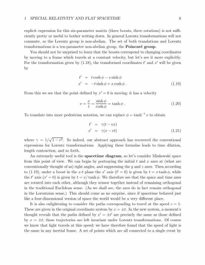
An extremely useful tool is the spacetime diagram, so let’s consider Minkowski space

from this point of view. We can begin by portraying the initial t and x axes at (what areconventionally thought of as) right angles, and suppressing the y and z axes. Then according

to (1.19), under a boost in the x-t plane the x! axis (t! = 0) is given by t = x tanh $, while

the t! axis (x! = 0) is given by t = x/ tanh $. We therefore see that the space and time axes

are rotated into each other, although they scissor together instead of remaining orthogonal

in the traditional Euclidean sense. (As we shall see, the axes do in fact remain orthogonal

in the Lorentzian sense.) This should come as no surprise, since if spacetime behaved justlike a four-dimensional version of space the world would be a very di!erent place.

It is also enlightening to consider the paths corresponding to travel at the speed c = 1.

These are given in the original coordinate system by x = ±t. In the new system, a moment’s

thought reveals that the paths defined by x! = ±t! are precisely the same as those defined

by x = ±t; these trajectories are left invariant under Lorentz transformations. Of course

we know that light travels at this speed; we have therefore found that the speed of light isthe same in any inertial frame. A set of points which are all connected to a single event by


x’

x

tt’

x = -tx’ = -t’

x = tx’ = t’

straight lines moving at the speed of light is called a light cone; this entire set is invariantunder Lorentz transformations. Light cones are naturally divided into future and past; the

set of all points inside the future and past light cones of a point p are called timelike

separated from p, while those outside the light cones are spacelike separated and those

on the cones are lightlike or null separated from p. Referring back to (1.3), we see that the

interval between timelike separated points is negative, between spacelike separated points is

positive, and between null separated points is zero. (The interval is defined to be s2, not thesquare root of this quantity.) Notice the distinction between this situation and that in the

Newtonian world; here, it is impossible to say (in a coordinate-independent way) whether a

point that is spacelike separated from p is in the future of p, the past of p, or “at the same

time”.

To probe the structure of Minkowski space in more detail, it is necessary to introduce

the concepts of vectors and tensors. We will start with vectors, which should be familiar. Ofcourse, in spacetime vectors are four-dimensional, and are often referred to as four-vectors.

This turns out to make quite a bit of di!erence; for example, there is no such thing as a

cross product between two four-vectors.

Beyond the simple fact of dimensionality, the most important thing to emphasize is that

each vector is located at a given point in spacetime. You may be used to thinking of vectors

as stretching from one point to another in space, and even of “free” vectors which you canslide carelessly from point to point. These are not useful concepts in relativity. Rather, to

each point p in spacetime we associate the set of all possible vectors located at that point;

this set is known as the tangent space at p, or Tp. The name is inspired by thinking of the

set of vectors attached to a point on a simple curved two-dimensional space as comprising a


plane which is tangent to the point. But inspiration aside, it is important to think of these

vectors as being located at a single point, rather than stretching from one point to another.(Although this won’t stop us from drawing them as arrows on spacetime diagrams.)

p

manifold

M

Tp

Later we will relate the tangent space at each point to things we can construct from thespacetime itself. For right now, just think of Tp as an abstract vector space for each point

in spacetime. A (real) vector space is a collection of objects (“vectors”) which, roughly

speaking, can be added together and multiplied by real numbers in a linear way. Thus, for

any two vectors V and W and real numbers a and b, we have

(a + b)(V + W ) = aV + bV + aW + bW . (1.22)

Every vector space has an origin, i.e. a zero vector which functions as an identity element

under vector addition. In many vector spaces there are additional operations such as takingan inner (dot) product, but this is extra structure over and above the elementary concept of

a vector space.

A vector is a perfectly well-defined geometric object, as is a vector field, defined as a

set of vectors with exactly one at each point in spacetime. (The set of all the tangent spaces

of a manifold M is called the tangent bundle, T (M).) Nevertheless it is often useful for

concrete purposes to decompose vectors into components with respect to some set of basisvectors. A basis is any set of vectors which both spans the vector space (any vector is

a linear combination of basis vectors) and is linearly independent (no vector in the basis

is a linear combination of other basis vectors). For any given vector space, there will be

an infinite number of legitimate bases, but each basis will consist of the same number of


vectors, known as the dimension of the space. (For a tangent space associated with a point

in Minkowski space, the dimension is of course four.)Let us imagine that at each tangent space we set up a basis of four vectors e(µ), with

µ & {0, 1, 2, 3} as usual. In fact let us say that each basis is adapted to the coordinates xµ;

that is, the basis vector e(1) is what we would normally think of pointing along the x-axis,

etc. It is by no means necessary that we choose a basis which is adapted to any coordinate

system at all, although it is often convenient. (We really could be more precise here, but

later on we will repeat the discussion at an excruciating level of precision, so some sloppinessnow is forgivable.) Then any abstract vector A can be written as a linear combination of

basis vectors:

A = Aµe(µ) . (1.23)

The coe"cients Aµ are the components of the vector A. More often than not we will forget

the basis entirely and refer somewhat loosely to “the vector Aµ”, but keep in mind thatthis is shorthand. The real vector is an abstract geometrical entity, while the components

are just the coe"cients of the basis vectors in some convenient basis. (Since we will usually

suppress the explicit basis vectors, the indices will usually label components of vectors and

tensors. This is why there are parentheses around the indices on the basis vectors, to remind

us that this is a collection of vectors, not components of a single vector.)

A standard example of a vector in spacetime is the tangent vector to a curve. A param-eterized curve or path through spacetime is specified by the coordinates as a function of the

parameter, e.g. xµ(&). The tangent vector V (&) has components

V µ =dxµ

d&. (1.24)

The entire vector is thus V = V µe(µ). Under a Lorentz transformation the coordinates

xµ change according to (1.11), while the parameterization & is unaltered; we can thereforededuce that the components of the tangent vector must change as

V µ # V µ!

= $µ!

!V! . (1.25)

However, the vector itself (as opposed to its components in some coordinate system) is

invariant under Lorentz transformations. We can use this fact to derive the transformationproperties of the basis vectors. Let us refer to the set of basis vectors in the transformed

coordinate system as e(!!). Since the vector is invariant, we have

V = V µe(µ) = V !!

e(!!)

= $!!

µVµe(!!) . (1.26)

But this relation must hold no matter what the numerical values of the components V µ are.Therefore we can say

e(µ) = $!!

µe(!!) . (1.27)


To get the new basis e(!!) in terms of the old one e(µ) we should multiply by the inverse

of the Lorentz transformation $!!

µ. But the inverse of a Lorentz transformation from theunprimed to the primed coordinates is also a Lorentz transformation, this time from the

primed to the unprimed systems. We will therefore introduce a somewhat subtle notation,

by writing using the same symbol for both matrices, just with primed and unprimed indices

adjusted. That is,

($"1)!!

µ = $!!µ , (1.28)

or

$!!µ$#!

µ = '#!

!! , $!!µ$!!

" = 'µ" , (1.29)

where 'µ" is the traditional Kronecker delta symbol in four dimensions. (Note that Schutz uses

a di!erent convention, always arranging the two indices northwest/southeast; the importantthing is where the primes go.) From (1.27) we then obtain the transformation rule for basis

vectors:

e(!!) = $!!µe(µ) . (1.30)

Therefore the set of basis vectors transforms via the inverse Lorentz transformation of thecoordinates or vector components.

It is worth pausing a moment to take all this in. We introduced coordinates labeled by

upper indices, which transformed in a certain way under Lorentz transformations. We then

considered vector components which also were written with upper indices, which made sense

since they transformed in the same way as the coordinate functions. (In a fixed coordinate

system, each of the four coordinates xµ can be thought of as a function on spacetime, ascan each of the four components of a vector field.) The basis vectors associated with the

coordinate system transformed via the inverse matrix, and were labeled by a lower index.

This notation ensured that the invariant object constructed by summing over the components

and basis vectors was left unchanged by the transformation, just as we would wish. It’s

probably not giving too much away to say that this will continue to be the case for more

complicated objects with multiple indices (tensors).

Once we have set up a vector space, there is an associated vector space (of equal dimen-sion) which we can immediately define, known as the dual vector space. The dual space

is usually denoted by an asterisk, so that the dual space to the tangent space Tp is called

the cotangent space and denoted T #p . The dual space is the space of all linear maps from

the original vector space to the real numbers; in math lingo, if ( & T #p is a dual vector, then

it acts as a map such that:

((aV + bW ) = a((V ) + b((W ) & R , (1.31)

where V , W are vectors and a, b are real numbers. The nice thing about these maps is that

they form a vector space themselves; thus, if ( and ! are dual vectors, we have

(a( + b!)(V ) = a((V ) + b!(V ) . (1.32)


To make this construction somewhat more concrete, we can introduce a set of basis dual

vectors "(!) by demanding"(!)(e(µ)) = '!

µ . (1.33)

Then every dual vector can be written in terms of its components, which we label with lower

indices:

( = (µ"(µ) . (1.34)

In perfect analogy with vectors, we will usually simply write (µ to stand for the entire dual

vector. In fact, you will sometime see elements of Tp (what we have called vectors) referred to

as contravariant vectors, and elements of T #p (what we have called dual vectors) referred

to as covariant vectors. Actually, if you just refer to ordinary vectors as vectors with upperindices and dual vectors as vectors with lower indices, nobody should be o!ended. Another

name for dual vectors is one-forms, a somewhat mysterious designation which will become

clearer soon.

The component notation leads to a simple way of writing the action of a dual vector on

a vector:

((V ) = (µV ! "(µ)(e(!))

= (µV !'µ!

= (µV µ & R . (1.35)

This is why it is rarely necessary to write the basis vectors (and dual vectors) explicitly; the

components do all of the work. The form of (1.35) also suggests that we can think of vectors

as linear maps on dual vectors, by defining

V (() ' ((V ) = (µVµ . (1.36)

Therefore, the dual space to the dual vector space is the original vector space itself.

Of course in spacetime we will be interested not in a single vector space, but in fields of

vectors and dual vectors. (The set of all cotangent spaces over M is the cotangent bundle,

T #(M).) In that case the action of a dual vector field on a vector field is not a single number,

but a scalar (or just “function”) on spacetime. A scalar is a quantity without indices, whichis unchanged under Lorentz transformations.

We can use the same arguments that we earlier used for vectors to derive the transfor-

mation properties of dual vectors. The answers are, for the components,

(µ! = $µ!!(! , (1.37)

and for basis dual vectors,

"("!) = $"!#"(#) . (1.38)


This is just what we would expect from index placement; the components of a dual vector

transform under the inverse transformation of those of a vector. Note that this ensures thatthe scalar (1.35) is invariant under Lorentz transformations, just as it should be.

Let’s consider some examples of dual vectors, first in other contexts and then in Minkowski

space. Imagine the space of n-component column vectors, for some integer n. Then the dual

space is that of n-component row vectors, and the action is ordinary matrix multiplication:

V =

!

""""""""#

V 1

V 2

···

V n

$

%%%%%%%%&

, ( = ((1 (2 · · · (n) ,

((V ) = ((1 (2 · · · (n)

!

""""""""#

V 1

V 2

···

V n

$

%%%%%%%%&

= (iVi . (1.39)

Another familiar example occurs in quantum mechanics, where vectors in the Hilbert space

are represented by kets, |)(. In this case the dual space is the space of bras, )$|, and theaction gives the number )$|)(. (This is a complex number in quantum mechanics, but the

idea is precisely the same.)

In spacetime the simplest example of a dual vector is the gradient of a scalar function,

the set of partial derivatives with respect to the spacetime coordinates, which we denote by

“d”:

d$ =*$

*xµ"(µ) . (1.40)

The conventional chain rule used to transform partial derivatives amounts in this case to the

transformation rule of components of dual vectors:

*$

*xµ!=

*xµ

*xµ!

*$

*xµ

= $µ!µ *$

*xµ, (1.41)

where we have used (1.11) and (1.28) to relate the Lorentz transformation to the coordinates.

The fact that the gradient is a dual vector leads to the following shorthand notations for

partial derivatives:*$

*xµ= *µ$ = $, µ . (1.42)


(Very roughly speaking, “xµ has an upper index, but when it is in the denominator of a

derivative it implies a lower index on the resulting object.”) I’m not a big fan of the commanotation, but we will use *µ all the time. Note that the gradient does in fact act in a natural

way on the example we gave above of a vector, the tangent vector to a curve. The result is

ordinary derivative of the function along the curve:

*µ$*xµ

*&=

d$

d&. (1.43)

As a final note on dual vectors, there is a way to represent them as pictures which is

consistent with the picture of vectors as arrows. See the discussion in Schutz, or in MTW

(where it is taken to dizzying extremes).

A straightforward generalization of vectors and dual vectors is the notion of a tensor.Just as a dual vector is a linear map from vectors to R, a tensor T of type (or rank) (k, l)

is a multilinear map from a collection of dual vectors and vectors to R:

T : T #p " · · ·" T #

p " Tp " · · ·" Tp # R

(k times) (l times) (1.44)

Here, “"” denotes the Cartesian product, so that for example Tp"Tp is the space of orderedpairs of vectors. Multilinearity means that the tensor acts linearly in each of its arguments;

for instance, for a tensor of type (1, 1), we have

T (a( + b!, cV + dW ) = acT ((, V ) + adT ((, W ) + bcT (!, V ) + bdT (!, W ) . (1.45)

From this point of view, a scalar is a type (0, 0) tensor, a vector is a type (1, 0) tensor, and

a dual vector is a type (0, 1) tensor.The space of all tensors of a fixed type (k, l) forms a vector space; they can be added

together and multiplied by real numbers. To construct a basis for this space, we need to

define a new operation known as the tensor product, denoted by *. If T is a (k, l) tensor

and S is a (m, n) tensor, we define a (k + m, l + n) tensor T * S by

T * S(((1), . . . , ((k), . . . , ((k+m), V (1), . . . , V (l), . . . , V (l+n))

= T (((1), . . . , ((k), V (1), . . . , V (l))S(((k+1), . . . , ((k+m), V (l+1), . . . , V (l+n)) . (1.46)

(Note that the ((i) and V (i) are distinct dual vectors and vectors, not components thereof.)

In other words, first act T on the appropriate set of dual vectors and vectors, and then act

S on the remainder, and then multiply the answers. Note that, in general, T * S += S * T .

It is now straightforward to construct a basis for the space of all (k, l) tensors, by taking

tensor products of basis vectors and dual vectors; this basis will consist of all tensors of theform

e(µ1) * · · ·* e(µk) * "(!1) * · · ·* "(!l) . (1.47)


In a 4-dimensional spacetime there will be 4k+l basis tensors in all. In component notation

we then write our arbitrary tensor as

T = T µ1···µk!1···!l

e(µ1) * · · ·* e(µk) * "(!1) * · · ·* "(!l) . (1.48)

Alternatively, we could define the components by acting the tensor on basis vectors and dual

vectors:T µ1···µk

!1···!l= T ("(µ1), . . . , "(µk), e(!1), . . . , e(!l)) . (1.49)

You can check for yourself, using (1.33) and so forth, that these equations all hang together

properly.As with vectors, we will usually take the shortcut of denoting the tensor T by its com-

ponents T µ1···µk!1···!l

. The action of the tensors on a set of vectors and dual vectors follows

the pattern established in (1.35):

T (((1), . . . , ((k), V (1), . . . , V (l)) = T µ1···µk!1···!l

((1)µ1

· · ·((k)µk

V (1)!1 · · ·V (l)!l . (1.50)

The order of the indices is obviously important, since the tensor need not act in the same way

on its various arguments. Finally, the transformation of tensor components under Lorentz

transformations can be derived by applying what we already know about the transformation

of basis vectors and dual vectors. The answer is just what you would expect from index

placement,T µ!

1···µ!

k !!

1···!!

l= $µ!

1µ1 · · ·$µ!

k µk$!!

1

!1 · · ·$!!

l

!lT µ1···µk!1···!l

. (1.51)

Thus, each upper index gets transformed like a vector, and each lower index gets transformedlike a dual vector.

Although we have defined tensors as linear maps from sets of vectors and tangent vectors

to R, there is nothing that forces us to act on a full collection of arguments. Thus, a (1, 1)

tensor also acts as a map from vectors to vectors:

T µ! : V ! # T µ

!V! . (1.52)

You can check for yourself that T µ!V ! is a vector (i.e. obeys the vector transformation law).

Similarly, we can act one tensor on (all or part of) another tensor to obtain a third tensor.

For example,

Uµ! = T µ"

#S#"! (1.53)

is a perfectly good (1, 1) tensor.

You may be concerned that this introduction to tensors has been somewhat too brief,

given the esoteric nature of the material. In fact, the notion of tensors does not require agreat deal of e!ort to master; it’s just a matter of keeping the indices straight, and the rules

for manipulating them are very natural. Indeed, a number of books like to define tensors as


collections of numbers transforming according to (1.51). While this is operationally useful, it

tends to obscure the deeper meaning of tensors as geometrical entities with a life independentof any chosen coordinate system. There is, however, one subtlety which we have glossed over.

The notions of dual vectors and tensors and bases and linear maps belong to the realm of

linear algebra, and are appropriate whenever we have an abstract vector space at hand. In

the case of interest to us we have not just a vector space, but a vector space at each point in

spacetime. More often than not we are interested in tensor fields, which can be thought of

as tensor-valued functions on spacetime. Fortunately, none of the manipulations we definedabove really care whether we are dealing with a single vector space or a collection of vector

spaces, one for each event. We will be able to get away with simply calling things functions

of xµ when appropriate. However, you should keep straight the logical independence of the

notions we have introduced and their specific application to spacetime and relativity.

Now let’s turn to some examples of tensors. First we consider the previous example of

column vectors and their duals, row vectors. In this system a (1, 1) tensor is simply a matrix,M i

j. Its action on a pair ((, V ) is given by usual matrix multiplication:

M((, V ) = ((1 (2 · · · (n)

!

""""""""#

M11 M1

2 · · · M1n

M21 M2

2 · · · M2n

· · · · · ·· · · · · ·· · · · · ·

Mn1 Mn

2 · · · Mnn

$

%%%%%%%%&

!

""""""""#

V 1

V 2

···

V n

$

%%%%%%%%&

= (iMijV

j . (1.54)

If you like, feel free to think of tensors as “matrices with an arbitrary number of indices.”

In spacetime, we have already seen some examples of tensors without calling them that.

The most familiar example of a (0, 2) tensor is the metric, !µ! . The action of the metric ontwo vectors is so useful that it gets its own name, the inner product (or dot product):

!(V, W ) = !µ!VµW ! = V · W . (1.55)

Just as with the conventional Euclidean dot product, we will refer to two vectors whose dot

product vanishes as orthogonal. Since the dot product is a scalar, it is left invariant under

Lorentz transformations; therefore the basis vectors of any Cartesian inertial frame, which

are chosen to be orthogonal by definition, are still orthogonal after a Lorentz transformation

(despite the “scissoring together” we noticed earlier). The norm of a vector is defined to be

inner product of the vector with itself; unlike in Euclidean space, this number is not positivedefinite:

if !µ!VµV ! is

'()

(*

< 0 , V µ is timelike= 0 , V µ is lightlike or null> 0 , V µ is spacelike .


(A vector can have zero norm without being the zero vector.) You will notice that the

terminology is the same as that which we earlier used to classify the relationship betweentwo points in spacetime; it’s no accident, of course, and we will go into more detail later.

Another tensor is the Kronecker delta 'µ! , of type (1, 1), which you already know the

components of. Related to this and the metric is the inverse metric !µ! , a type (2, 0)

tensor defined as the inverse of the metric:

!µ!!!" = !"!!!µ = '"µ . (1.56)

In fact, as you can check, the inverse metric has exactly the same components as the metric

itself. (This is only true in flat space in Cartesian coordinates, and will fail to hold in more

general situations.) There is also the Levi-Civita tensor, a (0, 4) tensor:

+µ!"# =

'()

(*

+1 if µ,-. is an even permutation of 0123!1 if µ,-. is an odd permutation of 01230 otherwise .

(1.57)

Here, a “permutation of 0123” is an ordering of the numbers 0, 1, 2, 3 which can be obtained

by starting with 0123 and exchanging two of the digits; an even permutation is obtained by

an even number of such exchanges, and an odd permutation is obtained by an odd number.

Thus, for example, +0321 = !1.

It is a remarkable property of the above tensors – the metric, the inverse metric, theKronecker delta, and the Levi-Civita tensor – that, even though they all transform according

to the tensor transformation law (1.51), their components remain unchanged in any Cartesian

coordinate system in flat spacetime. In some sense this makes them bad examples of tensors,

since most tensors do not have this property. In fact, even these tensors do not have this

property once we go to more general coordinate systems, with the single exception of the

Kronecker delta. This tensor has exactly the same components in any coordinate systemin any spacetime. This makes sense from the definition of a tensor as a linear map; the

Kronecker tensor can be thought of as the identity map from vectors to vectors (or from

dual vectors to dual vectors), which clearly must have the same components regardless of

coordinate system. The other tensors (the metric, its inverse, and the Levi-Civita tensor)

characterize the structure of spacetime, and all depend on the metric. We shall therefore

have to treat them more carefully when we drop our assumption of flat spacetime.A more typical example of a tensor is the electromagnetic field strength tensor. We

all know that the electromagnetic fields are made up of the electric field vector Ei and the

magnetic field vector Bi. (Remember that we use Latin indices for spacelike components

1,2,3.) Actually these are only “vectors” under rotations in space, not under the full Lorentz


group. In fact they are components of a (0, 2) tensor Fµ! , defined by

Fµ! =

!

"""#

0 !E1 !E2 !E3

E1 0 B3 !B2

E2 !B3 0 B1

E3 B2 !B1 0

$

%%%& = !F!µ . (1.58)

From this point of view it is easy to transform the electromagnetic fields in one referenceframe to those in another, by application of (1.51). The unifying power of the tensor formal-

ism is evident: rather than a collection of two vectors whose relationship and transformation

properties are rather mysterious, we have a single tensor field to describe all of electromag-

netism. (On the other hand, don’t get carried away; sometimes it’s more convenient to work

in a single coordinate system using the electric and magnetic field vectors.)

With some examples in hand we can now be a little more systematic about some prop-erties of tensors. First consider the operation of contraction, which turns a (k, l) tensor

into a (k ! 1, l! 1) tensor. Contraction proceeds by summing over one upper and one lower

index:

Sµ"# = T µ!"

#! . (1.59)

You can check that the result is a well-defined tensor. Of course it is only permissible to

contract an upper index with a lower index (as opposed to two indices of the same type).

Note also that the order of the indices matters, so that you can get di!erent tensors by

contracting in di!erent ways; thus,

T µ!"#! += T µ"!

#! (1.60)

in general.The metric and inverse metric can be used to raise and lower indices on tensors. That

is, given a tensor T $%&', we can use the metric to define new tensors which we choose to

denote by the same letter T :

T $%µ' = !µ&T $%

&' ,

Tµ%

&' = !µ$T $%&' ,

Tµ!"# = !µ$!!%!"&!#'T $%

&' , (1.61)

and so forth. Notice that raising and lowering does not change the position of an indexrelative to other indices, and also that “free” indices (which are not summed over) must be

the same on both sides of an equation, while “dummy” indices (which are summed over)

only appear on one side. As an example, we can turn vectors and dual vectors into each

other by raising and lowering indices:

Vµ = !µ!V!

(µ = !µ!(! . (1.62)


This explains why the gradient in three-dimensional flat Euclidean space is usually thought

of as an ordinary vector, even though we have seen that it arises as a dual vector; in Euclideanspace (where the metric is diagonal with all entries +1) a dual vector is turned into a vector

with precisely the same components when we raise its index. You may then wonder why we

have belabored the distinction at all. One simple reason, of course, is that in a Lorentzian

spacetime the components are not equal:

(µ = (!(0, (1, (2, (3) . (1.63)

In a curved spacetime, where the form of the metric is generally more complicated, the dif-

ference is rather more dramatic. But there is a deeper reason, namely that tensors generallyhave a “natural” definition which is independent of the metric. Even though we will always

have a metric available, it is helpful to be aware of the logical status of each mathematical

object we introduce. The gradient, and its action on vectors, is perfectly well defined re-

gardless of any metric, whereas the “gradient with upper indices” is not. (As an example,

we will eventually want to take variations of functionals with respect to the metric, and will

therefore have to know exactly how the functional depends on the metric, something that iseasily obscured by the index notation.)

Continuing our compilation of tensor jargon, we refer to a tensor as symmetric in any

of its indices if it is unchanged under exchange of those indices. Thus, if

Sµ!" = S!µ" , (1.64)

we say that Sµ!" is symmetric in its first two indices, while if

Sµ!" = Sµ"! = S"µ! = S!µ" = S!"µ = S"!µ , (1.65)

we say that Sµ!" is symmetric in all three of its indices. Similarly, a tensor is antisym-

metric (or “skew-symmetric”) in any of its indices if it changes sign when those indices are

exchanged; thus,

Aµ!" = !A"!µ (1.66)

means that Aµ!" is antisymmetric in its first and third indices (or just “antisymmetric in µ

and -”). If a tensor is (anti-) symmetric in all of its indices, we refer to it as simply (anti-)

symmetric (sometimes with the redundant modifier “completely”). As examples, the metric

!µ! and the inverse metric !µ! are symmetric, while the Levi-Civita tensor +µ!"# and the

electromagnetic field strength tensor Fµ! are antisymmetric. (Check for yourself that if youraise or lower a set of indices which are symmetric or antisymmetric, they remain that way.)

Notice that it makes no sense to exchange upper and lower indices with each other, so don’t

succumb to the temptation to think of the Kronecker delta '$% as symmetric. On the other

hand, the fact that lowering an index on '$% gives a symmetric tensor (in fact, the metric)


means that the order of indices doesn’t really matter, which is why we don’t keep track index

placement for this one tensor.Given any tensor, we can symmetrize (or antisymmetrize) any number of its upper or

lower indices. To symmetrize, we take the sum of all permutations of the relevant indices

and divide by the number of terms:

T(µ1µ2···µn)"# =

1

n!(Tµ1µ2···µn"

# + sum over permutations of indices µ1 · · ·µn) , (1.67)

while antisymmetrization comes from the alternating sum:

T[µ1µ2···µn]"# =

1

n!(Tµ1µ2···µn"

# + alternating sum over permutations of indices µ1 · · ·µn) .

(1.68)

By “alternating sum” we mean that permutations which are the result of an odd number ofexchanges are given a minus sign, thus:

T[µ!"]# =1

6(Tµ!"# ! Tµ"!# + T"µ!# ! T!µ"# + T!"µ# ! T"!µ#) . (1.69)

Notice that round/square brackets denote symmetrization/antisymmetrization. Further-

more, we may sometimes want to (anti-) symmetrize indices which are not next to each

other, in which case we use vertical bars to denote indices not included in the sum:

T(µ|!|") =1

2(Tµ!" + T"!µ) . (1.70)

Finally, some people use a convention in which the factor of 1/n! is omitted. The one used

here is a good one, since (for example) a symmetric tensor satisfies

Sµ1···µn = S(µ1···µn) , (1.71)

and likewise for antisymmetric tensors.We have been very careful so far to distinguish clearly between things that are always

true (on a manifold with arbitrary metric) and things which are only true in Minkowski

space in Cartesian coordinates. One of the most important distinctions arises with partial

derivatives. If we are working in flat spacetime with Cartesian coordinates, then the partial

derivative of a (k, l) tensor is a (k, l + 1) tensor; that is,

T$µ

! = *$Rµ! (1.72)

transforms properly under Lorentz transformations. However, this will no longer be true

in more general spacetimes, and we will have to define a “covariant derivative” to take theplace of the partial derivative. Nevertheless, we can still use the fact that partial derivatives


give us tensor in this special case, as long as we keep our wits about us. (The one exception

to this warning is the partial derivative of a scalar, *$$, which is a perfectly good tensor[the gradient] in any spacetime.)

We have now accumulated enough tensor know-how to illustrate some of these concepts

using actual physics. Specifically, we will examine Maxwell’s equations of electrodynam-

ics. In 19th-century notation, these are

," B! *tE = 4#J

, · E = 4#-

,"E + *tB = 0

, · B = 0 . (1.73)

Here, E and B are the electric and magnetic field 3-vectors, J is the current, - is the

charge density, and ," and ,· are the conventional curl and divergence. These equations

are invariant under Lorentz transformations, of course; that’s how the whole business got

started. But they don’t look obviously invariant; our tensor notation can fix that. Let’s

begin by writing these equations in just a slightly di!erent notation,

+ijk*jBk ! *0Ei = 4#J i

*iEi = 4#J0

+ijk*jEk + *0Bi = 0

*iBi = 0 . (1.74)

In these expressions, spatial indices have been raised and lowered with abandon, without

any attempt to keep straight where the metric appears. This is because 'ij is the metric on

flat 3-space, with 'ij its inverse (they are equal as matrices). We can therefore raise andlower indices at will, since the components don’t change. Meanwhile, the three-dimensional

Levi-Civita tensor +ijk is defined just as the four-dimensional one, although with one fewer

index. We have replaced the charge density by J0; this is legitimate because the density and

current together form the current 4-vector, Jµ = (-, J1, J2, J3).

From these expressions, and the definition (1.58) of the field strength tensor Fµ! , it is

easy to get a completely tensorial 20th-century version of Maxwell’s equations. Begin bynoting that we can express the field strength with upper indices as

F 0i = Ei

F ij = +ijkBk . (1.75)

(To check this, note for example that F 01 = !00!11F01 and F 12 = +123B3.) Then the first two

equations in (1.74) become

*jFij ! *0F

0i = 4#J i


*iF0i = 4#J0 . (1.76)

Using the antisymmetry of F µ! , we see that these may be combined into the single tensor

equation

*µF !µ = 4#J! . (1.77)

A similar line of reasoning, which is left as an exercise to you, reveals that the third and

fourth equations in (1.74) can be written

*[µF!(] = 0 . (1.78)

The four traditional Maxwell equations are thus replaced by two, thus demonstrating the

economy of tensor notation. More importantly, however, both sides of equations (1.77) and

(1.78) manifestly transform as tensors; therefore, if they are true in one inertial frame, they

must be true in any Lorentz-transformed frame. This is why tensors are so useful in relativity

— we often want to express relationships without recourse to any reference frame, and it is

necessary that the quantities on each side of an equation transform in the same way under

change of coordinates. As a matter of jargon, we will sometimes refer to quantities whichare written in terms of tensors as covariant (which has nothing to do with “covariant”

as opposed to “contravariant”). Thus, we say that (1.77) and (1.78) together serve as the

covariant form of Maxwell’s equations, while (1.73) or (1.74) are non-covariant.

Let us now introduce a special class of tensors, known as di!erential forms (or just

“forms”). A di!erential p-form is a (0, p) tensor which is completely antisymmetric. Thus,

scalars are automatically 0-forms, and dual vectors are automatically one-forms (thus ex-plaining this terminology from a while back). We also have the 2-form Fµ! and the 4-form

+µ!"#. The space of all p-forms is denoted $p, and the space of all p-form fields over a mani-

fold M is denoted $p(M). A semi-straightforward exercise in combinatorics reveals that the

number of linearly independent p-forms on an n-dimensional vector space is n!/(p!(n! p)!).

So at a point on a 4-dimensional spacetime there is one linearly independent 0-form, four

1-forms, six 2-forms, four 3-forms, and one 4-form. There are no p-forms for p > n, since allof the components will automatically be zero by antisymmetry.

Why should we care about di!erential forms? This is a hard question to answer without

some more work, but the basic idea is that forms can be both di!erentiated and integrated,

without the help of any additional geometric structure. We will delay integration theory

until later, but see how to di!erentiate forms shortly.

Given a p-form A and a q-form B, we can form a (p + q)-form known as the wedgeproduct A - B by taking the antisymmetrized tensor product:

(A - B)µ1···µp+q =(p + q)!

p! q!A[µ1···µpBµp+1···µp+q] . (1.79)


Thus, for example, the wedge product of two 1-forms is

(A - B)µ! = 2A[µB!] = AµB! ! A!Bµ . (1.80)

Note that

A - B = (!1)pqB - A , (1.81)

so you can alter the order of a wedge product if you are careful with signs.

The exterior derivative “d” allows us to di!erentiate p-form fields to obtain (p+1)-form

fields. It is defined as an appropriately normalized antisymmetric partial derivative:

(dA)µ1···µp+1 = (p + 1)*[µ1Aµ2···µp+1] . (1.82)

The simplest example is the gradient, which is the exterior derivative of a 1-form:

(d$)µ = *µ$ . (1.83)

The reason why the exterior derivative deserves special attention is that it is a tensor, even in

curved spacetimes, unlike its cousin the partial derivative. Since we haven’t studied curved

spaces yet, we cannot prove this, but (1.82) defines an honest tensor no matter what the

metric and coordinates are.Another interesting fact about exterior di!erentiation is that, for any form A,

d(dA) = 0 , (1.84)

which is often written d2 = 0. This identity is a consequence of the definition of d and the

fact that partial derivatives commute, *$*% = *%*$ (acting on anything). This leads us to

the following mathematical aside, just for fun. We define a p-form A to be closed if dA = 0,

and exact if A = dB for some (p!1)-form B. Obviously, all exact forms are closed, but theconverse is not necessarily true. On a manifold M , closed p-forms comprise a vector space

Zp(M), and exact forms comprise a vector space Bp(M). Define a new vector space as the

closed forms modulo the exact forms:

Hp(M) =Zp(M)

Bp(M). (1.85)

This is known as the pth de Rham cohomology vector space, and depends only on the

topology of the manifold M . (Minkowski space is topologically equivalent to R4, which is

uninteresting, so that all of the Hp(M) vanish for p > 0; for p = 0 we have H0(M) = R.

Therefore in Minkowski space all closed forms are exact except for zero-forms; zero-forms

can’t be exact since there are no !1-forms for them to be the exterior derivative of.) It isstriking that information about the topology can be extracted in this way, which essentially

involves the solutions to di!erential equations. The dimension bp of the space Hp(M) is


called the pth Betti number of M , and the Euler characteristic is given by the alternating

sum

/(M) =n+

p=0

(!1)pbp . (1.86)

Cohomology theory is the basis for much of modern di!erential topology.Moving back to reality, the final operation on di!erential forms we will introduce is

Hodge duality. We define the “Hodge star operator” on an n-dimensional manifold as a

map from p-forms to (n ! p)-forms,

(.A)µ1···µn"p =1

p!+!1···!p

µ1···µn"pA!1···!p , (1.87)

mapping A to “A dual”. Unlike our other operations on forms, the Hodge dual does depend

on the metric of the manifold (which should be obvious, since we had to raise some indices

on the Levi-Civita tensor in order to define (1.87)). Applying the Hodge star twice returns

either plus or minus the original form:

. .A = (!1)s+p(n"p)A , (1.88)

where s is the number of minus signs in the eigenvalues of the metric (for Minkowski space,

s = 1).Two facts on the Hodge dual: First, “duality” in the sense of Hodge is di!erent than the

relationship between vectors and dual vectors, although both can be thought of as the space

of linear maps from the original space to R. Notice that the dimensionality of the space of

(n ! p)-forms is equal to that of the space of p-forms, so this has at least a chance of being

true. In the case of forms, the linear map defined by an (n ! p)-form acting on a p-form is

given by the dual of the wedge product of the two forms. Thus, if A(n"p) is an (n ! p)-formand B(p) is a p-form at some point in spacetime, we have

. (A(n"p) - B(p)) & R . (1.89)

The second fact concerns di!erential forms in 3-dimensional Euclidean space. The Hodge

dual of the wedge product of two 1-forms gives another 1-form:

. (U - V )i = +ijkUjVk . (1.90)

(All of the prefactors cancel.) Since 1-forms in Euclidean space are just like vectors, we have

a map from two vectors to a single vector. You should convince yourself that this is just the

conventional cross product, and that the appearance of the Levi-Civita tensor explains why

the cross product changes sign under parity (interchange of two coordinates, or equivalentlybasis vectors). This is why the cross product only exists in three dimensions — because only


in three dimensions do we have an interesting map from two dual vectors to a third dual

vector. If you wanted to you could define a map from n ! 1 one-forms to a single one-form,but I’m not sure it would be of any use.

Electrodynamics provides an especially compelling example of the use of di!erential

forms. From the definition of the exterior derivative, it is clear that equation (1.78) can

be concisely expressed as closure of the two-form Fµ! :

dF = 0 . (1.91)

Does this mean that F is also exact? Yes; as we’ve noted, Minkowski space is topologically

trivial, so all closed forms are exact. There must therefore be a one-form Aµ such that

F = dA . (1.92)

This one-form is the familiar vector potential of electromagnetism, with the 0 componentgiven by the scalar potential, A0 = $. If one starts from the view that the Aµ is the

fundamental field of electromagnetism, then (1.91) follows as an identity (as opposed to a

dynamical law, an equation of motion). Gauge invariance is expressed by the observation

that the theory is invariant under A # A + d& for some scalar (zero-form) &, and this is

also immediate from the relation (1.92). The other one of Maxwell’s equations, (1.77), can

be expressed as an equation between three-forms:

d(.F ) = 4#(.J) , (1.93)

where the current one-form J is just the current four-vector with index lowered. Filling in

the details is left for you to do.

As an intriguing aside, Hodge duality is the basis for one of the hottest topics in theoretical

physics today. It’s hard not to notice that the equations (1.91) and (1.93) look very similar.

Indeed, if we set Jµ = 0, the equations are invariant under the “duality transformations”

F # .F ,

.F # !F . (1.94)

We therefore say that the vacuum Maxwell’s equations are duality invariant, while the invari-

ance is spoiled in the presence of charges. We might imagine that magnetic as well as electric

monopoles existed in nature; then we could add a magnetic current term 4#(.JM) to the

right hand side of (1.91), and the equations would be invariant under duality transformations

plus the additional replacement J / JM . (Of course a nonzero right hand side to (1.91) is

inconsistent with F = dA, so this idea only works if Aµ is not a fundamental variable.) Longago Dirac considered the idea of magnetic monopoles and showed that a necessary condition

for their existence is that the fundamental monopole charge be inversely proportional to


the fundamental electric charge. Now, the fundamental electric charge is a small number;

electrodynamics is “weakly coupled”, which is why perturbation theory is so remarkablysuccessful in quantum electrodynamics (QED). But Dirac’s condition on magnetic charges

implies that a duality transformation takes a theory of weakly coupled electric charges to a

theory of strongly coupled magnetic monopoles (and vice-versa). Unfortunately monopoles

don’t exist (as far as we know), so these ideas aren’t directly applicable to electromagnetism;

but there are some theories (such as supersymmetric non-abelian gauge theories) for which

it has been long conjectured that some sort of duality symmetry may exist. If it did, wewould have the opportunity to analyze a theory which looked strongly coupled (and therefore

hard to solve) by looking at the weakly coupled dual version. Recently work by Seiberg and

Witten and others has provided very strong evidence that this is exactly what happens in

certain theories. The hope is that these techniques will allow us to explore various phenom-

ena which we know exist in strongly coupled quantum field theories, such as confinement of

quarks in hadrons.We’ve now gone over essentially everything there is to know about the care and feeding of

tensors. In the next section we will look more carefully at the rigorous definitions of manifolds

and tensors, but the basic mechanics have been pretty well covered. Before jumping to more

abstract mathematics, let’s review how physics works in Minkowski spacetime.

Start with the worldline of a single particle. This is specified by a map R # M , where

M is the manifold representing spacetime; we usually think of the path as a parameterized

curve xµ(&). As mentioned earlier, the tangent vector to this path is dxµ/d& (note that itdepends on the parameterization). An object of primary interest is the norm of the tangent

vector, which serves to characterize the path; if the tangent vector is timelike/null/spacelike

at some parameter value &, we say that the path is timelike/null/spacelike at that point. This

explains why the same words are used to classify vectors in the tangent space and intervals

between two points — because a straight line connecting, say, two timelike separated points

will itself be timelike at every point along the path.Nevertheless, it’s important to be aware of the sleight of hand which is being pulled here.

The metric, as a (0, 2) tensor, is a machine which acts on two vectors (or two copies of the

same vector) to produce a number. It is therefore very natural to classify tangent vectors

according to the sign of their norm. But the interval between two points isn’t something

quite so natural; it depends on a specific choice of path (a “straight line”) which connects

the points, and this choice in turn depends on the fact that spacetime is flat (which allowsa unique choice of straight line between the points). A more natural object is the line

element, or infinitesimal interval:

ds2 = !µ!dxµdx! . (1.95)

From this definition it is tempting to take the square root and integrate along a path to

obtain a finite interval. But since ds2 need not be positive, we define di!erent procedures


t

x

spacelike

null

timelike

dx--d

x ( )

λ

µ

µλ

for di!erent cases. For spacelike paths we define the path length

#s =, -

!µ!dxµ

d&

dx!

d&d& , (1.96)

where the integral is taken over the path. For null paths the interval is zero, so no extra

formula is required. For timelike paths we define the proper time

#0 =, -

!!µ!dxµ

d&

dx!

d&d& , (1.97)

which will be positive. Of course we may consider paths that are timelike in some places and

spacelike in others, but fortunately it is seldom necessary since the paths of physical particles

never change their character (massive particles move on timelike paths, massless particles

move on null paths). Furthermore, the phrase “proper time” is especially appropriate, since

0 actually measures the time elapsed on a physical clock carried along the path. This point ofview makes the “twin paradox” and similar puzzles very clear; two worldlines, not necessarily

straight, which intersect at two di!erent events in spacetime will have proper times measured

by the integral (1.97) along the appropriate paths, and these two numbers will in general be

di!erent even if the people travelling along them were born at the same time.

Let’s move from the consideration of paths in general to the paths of massive particles

(which will always be timelike). Since the proper time is measured by a clock travelling on

a timelike worldline, it is convenient to use 0 as the parameter along the path. That is, weuse (1.97) to compute 0(&), which (if & is a good parameter in the first place) we can invert

to obtain &(0), after which we can think of the path as xµ(0). The tangent vector in this


parameterization is known as the four-velocity, Uµ:

Uµ =dxµ

d0. (1.98)

Since d0 2 = !!µ!dxµdx! , the four-velocity is automatically normalized:

!µ!UµU! = !1 . (1.99)

(It will always be negative, since we are only defining it for timelike trajectories. You could

define an analogous vector for spacelike paths as well; null paths give some extra problems

since the norm is zero.) In the rest frame of a particle, its four-velocity has components

Uµ = (1, 0, 0, 0).

A related vector is the energy-momentum four-vector, defined by

pµ = mUµ , (1.100)

where m is the mass of the particle. The mass is a fixed quantity independent of inertial

frame; what you may be used to thinking of as the “rest mass.” It turns out to be muchmore convenient to take this as the mass once and for all, rather than thinking of mass as

depending on velocity. The energy of a particle is simply p0, the timelike component of its

energy-momentum vector. Since it’s only one component of a four-vector, it is not invariant

under Lorentz transformations; that’s to be expected, however, since the energy of a particle

at rest is not the same as that of the same particle in motion. In the particle’s rest frame we

have p0 = m; recalling that we have set c = 1, we find that we have found the equation that

made Einstein a celebrity, E = mc2. (The field equations of general relativity are actuallymuch more important than this one, but “Rµ! ! 1

2Rgµ! = 8#GTµ!” doesn’t elicit the visceral

reaction that you get from “E = mc2”.) In a moving frame we can find the components of

pµ by performing a Lorentz transformation; for a particle moving with (three-) velocity v

along the x axis we have

pµ = (%m, v%m, 0, 0) , (1.101)

where % = 1/%

1 ! v2. For small v, this gives p0 = m + 12mv2 (what we usually think of

as rest energy plus kinetic energy) and p1 = mv (what we usually think of as [Newtonian]momentum). So the energy-momentum vector lives up to its name.

The centerpiece of pre-relativity physics is Newton’s 2nd Law, or f = ma = dp/dt. An

analogous equation should hold in SR, and the requirement that it be tensorial leads us

directly to introduce a force four-vector fµ satisfying

fµ = md2

d0 2xµ(0) =

d

d0pµ(0) . (1.102)

The simplest example of a force in Newtonian physics is the force due to gravity. In relativity,

however, gravity is not described by a force, but rather by the curvature of spacetime itself.


Instead, let us consider electromagnetism. The three-dimensional Lorentz force is given

by f = q(E + v " B), where q is the charge on the particle. We would like a tensorialgeneralization of this equation. There turns out to be a unique answer:

fµ = qU(F(µ . (1.103)

You can check for yourself that this reduces to the Newtonian version in the limit of small

velocities. Notice how the requirement that the equation be tensorial, which is one way of

guaranteeing Lorentz invariance, severely restricted the possible expressions we could get.

This is an example of a very general phenomenon, in which a small number of an apparently

endless variety of possible physical laws are picked out by the demands of symmetry.

Although pµ provides a complete description of the energy and momentum of a particle,for extended systems it is necessary to go further and define the energy-momentum tensor

(sometimes called the stress-energy tensor), T µ! . This is a symmetric (2, 0) tensor which tells

us all we need to know about the energy-like aspects of a system: energy density, pressure,

stress, and so forth. A general definition of T µ! is “the flux of four-momentum pµ across a

surface of constant x!”. To make this more concrete, let’s consider the very general category

of matter which may be characterized as a fluid — a continuum of matter described bymacroscopic quantities such as temperature, pressure, entropy, viscosity, etc. In fact this

definition is so general that it is of little use. In general relativity essentially all interesting

types of matter can be thought of as perfect fluids, from stars to electromagnetic fields to

the entire universe. Schutz defines a perfect fluid to be one with no heat conduction and no

viscosity, while Weinberg defines it as a fluid which looks isotropic in its rest frame; these

two viewpoints turn out to be equivalent. Operationally, you should think of a perfect fluidas one which may be completely characterized by its pressure and density.

To understand perfect fluids, let’s start with the even simpler example of dust. Dust

is defined as a collection of particles at rest with respect to each other, or alternatively

as a perfect fluid with zero pressure. Since the particles all have an equal velocity in any

fixed inertial frame, we can imagine a “four-velocity field” Uµ(x) defined all over spacetime.

(Indeed, its components are the same at each point.) Define the number-flux four-vectorto be

Nµ = nUµ , (1.104)

where n is the number density of the particles as measured in their rest frame. Then N0

is the number density of particles as measured in any other frame, while N i is the flux of

particles in the xi direction. Let’s now imagine that each of the particles have the same mass

m. Then in the rest frame the energy density of the dust is given by

- = nm . (1.105)


By definition, the energy density completely specifies the dust. But - only measures the

energy density in the rest frame; what about other frames? We notice that both n andm are 0-components of four-vectors in their rest frame; specifically, Nµ = (n, 0, 0, 0) and

pµ = (m, 0, 0, 0). Therefore - is the µ = 0, , = 0 component of the tensor p*N as measured

in its rest frame. We are therefore led to define the energy-momentum tensor for dust:

T µ!dust = pµN! = nmUµU! = -UµU! , (1.106)

where - is defined as the energy density in the rest frame.

Having mastered dust, more general perfect fluids are not much more complicated. Re-

member that “perfect” can be taken to mean “isotropic in its rest frame.” This in turn

means that T µ! is diagonal — there is no net flux of any component of momentum in anorthogonal direction. Furthermore, the nonzero spacelike components must all be equal,

T 11 = T 22 = T 33. The only two independent numbers are therefore T 00 and one of the T ii;

we can choose to call the first of these the energy density -, and the second the pressure

p. (Sorry that it’s the same letter as the momentum.) The energy-momentum tensor of a

perfect fluid therefore takes the following form in its rest frame:

T µ! =

!

"""#

- 0 0 00 p 0 00 0 p 00 0 0 p

$

%%%& . (1.107)

We would like, of course, a formula which is good in any frame. For dust we had T µ! =

-UµU! , so we might begin by guessing (- + p)UµU! , which gives

!

"""#

- + p 0 0 00 0 0 00 0 0 00 0 0 0

$

%%%& . (1.108)

To get the answer we want we must therefore add!

"""#

!p 0 0 00 p 0 00 0 p 00 0 0 p

$

%%%& . (1.109)

Fortunately, this has an obvious covariant generalization, namely p!µ! . Thus, the general

form of the energy-momentum tensor for a perfect fluid is

T µ! = (- + p)UµU! + p!µ! . (1.110)

This is an important formula for applications such as stellar structure and cosmology.


As further examples, let’s consider the energy-momentum tensors of electromagnetism

and scalar field theory. Without any explanation at all, these are given by

T µ!e+m =

!1

4#(F µ(F !

( ! 1

4!µ!F (#F(#) , (1.111)

and

T µ!scalar = !µ(!!#*($*#$ ! 1

2!µ!(!(#*($*#$ + m2$2) . (1.112)

You can check for yourself that, for example, T 00 in each case is equal to what you would

expect the energy density to be.

Besides being symmetric, T µ! has the even more important property of being conserved.

In this context, conservation is expressed as the vanishing of the “divergence”:

*µTµ! = 0 . (1.113)

This is a set of four equations, one for each value of ,. The , = 0 equation corresponds to

conservation of energy, while *µT µk = 0 expresses conservation of the kth component of themomentum. We are not going to prove this in general; the proof follows for any individual

source of matter from the equations of motion obeyed by that kind of matter. In fact, one

way to define T µ! would be “a (2, 0) tensor with units of energy per volume, which is con-

served.” You can prove conservation of the energy-momentum tensor for electromagnetism,

for example, by taking the divergence of (1.111) and using Maxwell’s equations as previously

discussed.

A final aside: we have already mentioned that in general relativity gravitation does notcount as a “force.” As a related point, the gravitational field also does not have an energy-

momentum tensor. In fact it is very hard to come up with a sensible local expression for the

energy of a gravitational field; a number of suggestions have been made, but they all have

their drawbacks. Although there is no “correct” answer, it is an important issue from the

point of view of asking seemingly reasonable questions such as “What is the energy emitted

per second from a binary pulsar as the result of gravitational radiation?”

Date post:	01-Apr-2018
Category:	Documents
Upload:	hanga
View:	218 times
Download:	1 times

Lecture Notes on General Relativity - Sean Carroll · Wald, Weinberg, and Misner, Thorne and...

Documents