Lecture notes on introduction to tensors

K. M. UdayanandanAssociate Professor

Department of PhysicsNehru Arts and Science College, Kanhangad

1

.

Syllabus

Tensor analysis-Introduction-definition-definition of different rank

tensors-Contraction and direct product-quotient rule-pseudo tensors-

General tensors-Metric tensors

Contents

1 Introducing Tensors 4

1.1 Scalars or Vectors ? . . . . . . . . . . . . . . . . . . . . . . . . 5

1.2 Vector Division . . . . . . . . . . . . . . . . . . . . . . . . . . 6

1.3 Moment of inertia . . . . . . . . . . . . . . . . . . . . . . . . . 9

2 Re defining scalars and vectors 12

2.1 Cartesian Tensors . . . . . . . . . . . . . . . . . . . . . . . . . 13

2.1.1 Scalars . . . . . . . . . . . . . . . . . . . . . . . . . . . 13

2.1.2 Vectors . . . . . . . . . . . . . . . . . . . . . . . . . . . 13

2.1.3 Tensors . . . . . . . . . . . . . . . . . . . . . . . . . . 17

2.1.4 Summation Convention . . . . . . . . . . . . . . . . . . 18

3 Quotient Rule 20

4 Non-Cartesian Tensors-Metric Tensors 25

3

4.1 Spherical Polar Co-ordinate System . . . . . . . . . . . . . . . 25

4.2 Cylindrical coordinate system . . . . . . . . . . . . . . . . . . 28

5 Algebraic Operation of Tensors 30

5.0.1 Definition of Contravariant and Co variant vector . . . 30

5.0.2 Exercises . . . . . . . . . . . . . . . . . . . . . . . . . . 31

5.0.3 Co variant vector . . . . . . . . . . . . . . . . . . . . . 32

5.1 Addition & Subtraction of Tensors . . . . . . . . . . . . . . . 32

5.2 Symmetric and Anti symmetric Tensors . . . . . . . . . . . . . 32

5.3 Problems . . . . . . . . . . . . . . . . . . . . . . . . . . . . . 33

5.4 Contraction, Outer Product or Direct Product . . . . . . . . . 34

6 Pseudo Scalars and Pseudo Vectors and Pseudo Tensors 37

6.1 Pseudo Vectors . . . . . . . . . . . . . . . . . . . . . . . . . . 37

6.2 Pseudo scalars . . . . . . . . . . . . . . . . . . . . . . . . . . . 39

6.3 General Definition . . . . . . . . . . . . . . . . . . . . . . . . 39

6.4 Pseudo Tensor . . . . . . . . . . . . . . . . . . . . . . . . . . . 39

7 University Questions-Solved 44

Chapter 1

Introducing Tensors

In our daily life we see large number of physical quantities. Tensor is the

mathematical tool used to express these physical quantities. Any physi-

cal property that can be quantified is called a physical quantity. The

important property of a physical quantity is that it can be measured and

expressed in terms of a mathematical quantity like number. For example,

”length” is a physical quantity that can be expressed by stating a number

of some basic measurement unit such as meters, while ”anger” is a property

that is difficult to describe with a number. Hence we will not call ’anger’ or

’happiness’ as a physical quantity. The physical quantities so far identified

in physics are given below. Carefully read them. While reading observe that

some are expressed unbold, some are bold fonted and some are large and

bold. The known physical quantities are absorbed dose rate, acceleration,

angular acceleration, angular speed, angular momentum, area, area

density, capacitance, catalytic activity, chemical potential, molar concentra-

tion, current density, dynamic viscosity, electric charge, electric charge

5

density, electric displacement, electric field strength, electrical con-

ductance, electric potential, electrical resistance, energy, energy density,

entropy, force, frequency, half-life, heat, heat capacity, heat flux density, il-

luminate, impedance, index of refraction, inductance, irradiance, linear

density, luminous flux, magnetic field strength, magnetic flux, magnetic

flux density, magnetization, mass fraction, (mass) Density, mean lifetime,

molar energy, molar entropy, molar heat capacity, moment of iner-

tia, momentum,permeability, permittivity, power, pres-

sure, (radioactive) activity, (radioactive) dose, radiance, radiant intensity,

reaction rate, speed, specific energy, specific heat capacity, specific volume,

spin, stress, surface tension, thermal conductivity, torque, velocity, vol-

ume, wavelength, wave number, weight and work. Every physical quantity

must have a mathematical representation and only then a detailed study of

these will be s possible. Hence we have mathematical tools like theory of

numbers and vectors with which we can handle large number of physical

quantities.

1.1 Scalars or Vectors ?

Among the above physical quantities small bold faced quantities are vectors

and un bold are scalars. Generally we say quantities with magnitude only

as scalars and with magnitude and direction as vectors. But there are some

quantities which are given in large font which are not scalars and vectors.

If they are not scalars and vectors what are they? What is special

about these quantities ?. Let us have a look at it. One quality of the

above mentioned odd members is that some like mass, index of refraction,

6

permeability, permittivity sometimes behave as scalars and some times not.

The above mentioned physical quantities like mass, susceptibility. moment

of inertia, permeability and permittivity obey very familiar equations like.

~F = m~a, ~P = χ~E, ~L = I~ω, ~B = µ ~H, ~D = ε ~E, ~F = T ~A, ~J = σ ~E

from which we can write

m =~F

~a

χ =~P

~E

I =~L

~ω

etc. Consider the last case. Let ~L = 5i+5j+5k and ~ω = i+ j+ k. If you find

moment of inertia in this case you will get it as 5. But if ~L = 9i+ 4j + 11k

and ω is not changed we will not be able to divide ~L with ~ω and get the

moment of inertia. Why this happen? What mathematical quantity is

mass, susceptibility or moment of inertia? To understand this we must have

a look at the concept of vector division once again.

1.2 Vector Division

Consider a ball thrown vertically downwards into water with a velocity

~v = 6k

7

After entering water the velocity is decreased but the direction may not

change. Then the new velocity may be

~v′ = 3k = 0.5 ~v

Thus we transform the old velocity to a new velocity by a scalar multiple.

But this is not true in all cases. Suppose the ball is thrown at an angle then

the incident velocity may look like

~v = 5i+ 6j + 8k

and the deviated ball in the water may have different possible velocity like

~v′ = 3i+ 2j + 5k

~v′ = 2i+ 6j + 7k

etc. Consider the first case. The components of the final vector (3,2,5) can

be obtained in different ways. Among them some are given below.

3

2

5

=

35

0 0

0 13

0

0 0 58

5

6

8

The above transformation matrix is diagonal.

3

2

5

=

35

0 0

25

0 0

0 56

0

5

6

8

8

This transformation matrix is not diagonal.3

2

5

=

35−1 6

8

25

86−1

1 1 −68

5

6

8

Such a 3 × 3 with all elements non-zero can also be used to transform the

old velocity to new one. Or in general

v′x

v′y

v′z

=

v11 v12 v13

v21 v22 v23

v31 v32 v33

vx

vy

vz

This is the most general matrix which can be used to transform the

incident velocity to the new velocity. This shows that any vector can be

transformed to a new vector generally only by a 3 × 3 matrix in 3D. If the

matrix is diagonal and if the diagonal elements are same it becomes a scalar

multiple. We had seen that all our odd physical quantities always transform

one vector to a new vector. Hence the general form of these transforming

quantities must be a matrix with 9 components. Let us check whether this

is true with a specific example. For this let us find out what is the exact

nature of moment of inertia.

9

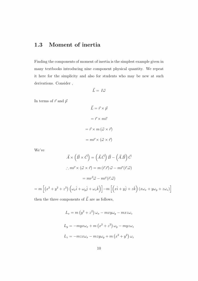
1.3 Moment of inertia

Finding the components of moment of inertia is the simplest example given in

many textbooks introducing nine component physical quantity. We repeat

it here for the simplicity and also for students who may be new at such

derivations. Consider ,

~L = I~ω

In terms of ~r and ~p

~L = ~r × ~p

= ~r ×m~v

= ~r ×m (~ω × ~r)

= m~r × (~ω × ~r)

We’ve

~A×(~B × ~C

)=(~A. ~C

)~B −

(~A. ~B

)~C

∴ m~r × (~ω × ~r) = m (~r.~r) ~ω −m~r (~r.~ω)

= mr2~ω −m~r (~r.~ω)

= m[(x2 + y2 + z2

) (ωxi+ ωy j + ωzk

)]−m

[(xi+ yj + zk

)(xωx + yωy + zωz)

]then the three components of ~L are as follows,

Lx = m(y2 + z2

)ωx −mxyωy −mxzωz

Ly = −myxωx +m(x2 + z2

)ωy −myzωz

Lz = −mzxωx −mzyωy +m(x2 + y2

)ωz

10

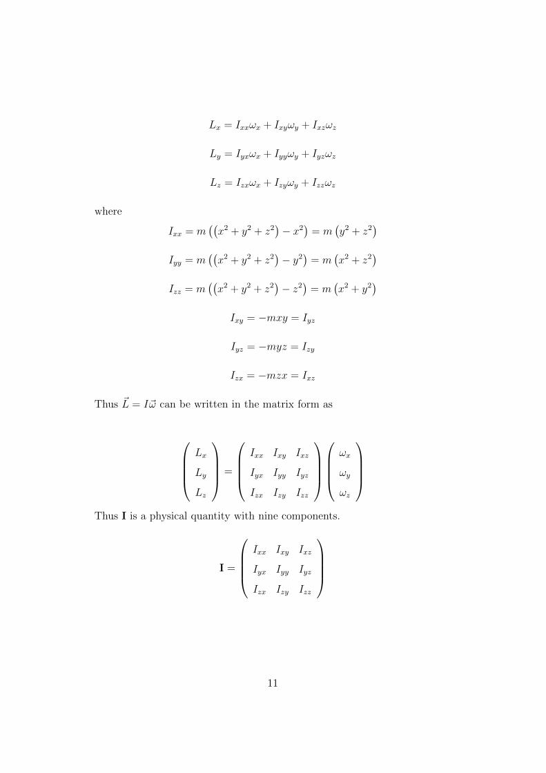
Lx = Ixxωx + Ixyωy + Ixzωz

Ly = Iyxωx + Iyyωy + Iyzωz

Lz = Izxωx + Izyωy + Izzωz

where

Ixx = m((x2 + y2 + z2

)− x2

)= m

(y2 + z2

)Iyy = m

((x2 + y2 + z2

)− y2

)= m

(x2 + z2

)Izz = m

((x2 + y2 + z2

)− z2

)= m

(x2 + y2

)Ixy = −mxy = Iyz

Iyz = −myz = Izy

Izx = −mzx = Ixz

Thus ~L = I~ω can be written in the matrix form as

Lx

Ly

Lz

=

Ixx Ixy Ixz

Iyx Iyy Iyz

Izx Izy Izz

ωx

ωy

ωz

Thus I is a physical quantity with nine components.

I =

Ixx Ixy Ixz

Iyx Iyy Iyz

Izx Izy Izz

11

I =

I11 I12 I13

I21 I22 I23

I31 I32 I33

Thus

Lx

Ly

Lz

=

m (y2 + z2) −mxy −mxz

−myx m (x2 + z2) −myz

−mzx −mzy m (x2 + y2)

ωx

ωy

ωz

In general we can write a componet as

Ii,j = m[r2δij − ri rj]

where i and j varies from 1 to 3 and r1 = x, r2 = y, r3 = z and r2 =

x2 + y2 + x2.

12

Chapter 2

Re defining scalars and vectors

We can see that scalars have one(30) component, vectors have 3 (31) com-

ponets and tensors we saw had 9 (32) components. This shows that all these

mathematical quantities belong to a family in 3 dimensional world. Hence

these three types of physical quantities must have a common type of defi-

nition. Since we classify them based on components we will redefine them

based on componets. Hence we can redefine the scalars and vectors using

coordinate transformation of components.

If the coordinate transformation is from cartesian to cartesian we call

all the quantities as cartesian tensors and if the transformation is from carte-

sian to spherical polar or cylindrical we call them as non cartesian tensors.

First we will study cartesian tensors.

13

2.1 Cartesian Tensors

2.1.1 Scalars

Under co-ordinate transformation, a scalar quantity has no change. ie When

we measure a scalar from a Cartesian or a rotated cartesian coordinate system

the value of scalar remains invariant Hence

S ′ = S

For if we measure mass of some substance say sugar standing straight and

then slightly tilting we will get the same mass. Thus any invariant quantity

under coordinate transformation is defined as a scalar.

2.1.2 Vectors

Consider a transformation from Cartesian to Cartesian coordinate systems.

Consider X1&X2 represent the unrotated co-ordinate system and X′1&X

′2

represent the rotated co-ordinate system. Let r be a vector and φ be the

angle between x1 axis and ~r. Then x1 = r cosφ and x2 = r sinφ. Let the

coordinates be rotated through an angle θ. Then

x′

1 = r cos (φ− θ) = r (cosφ cos θ + sinφ sin θ)

x′

2 = r sin (φ− θ) = r (sinφ cos θ − cosφ sin θ)

x′

1 = x1 cos θ + x2 sin θ

14

x′

2 = −x1 sin θ + x2 cos θ

In matrix form

x′1

x′2

=

cos θ sin θ

− sin θ cos θ

x1

x2

generally,

x′

i =∑j

aijxj

where i is 1 and 2 and j varies from 1 to 2.

x′

1 = a11x1 + a12x2

x′

2 = a21x1 + a22x2

Comparing

a11 = cos θ; a12 = sin θ

a21 = − sin θ; a22 = cos θ

Here we had taken position vector and performed transformation. Similarly

any vector can be transformed like this. Hence we can say a physical quantity

can be called as a vector if it obeys the transformation equation similar to

the transformation equation

x′

i =∑j

aijxj

Taking partial differential

15

∂x′1

∂x1= a11

∂x′1

∂x2= a12

∂x′2

∂x1= a21

∂x′2

∂x2= a22

Thus the transformation equation can also be written as

x′

i =∑j

∂x′i

∂xjxj

This is also the transformation equation for a vector. Let us proceed and find

the transformation from primed to unprimed coordinate system. We know

that for transformation from from X to X’ x′1

x′2

=

cos θ sin θ

− sin θ cos θ

x1

x2

x′1

x′2

= A

x1

x2

where

A =

cos θ sin θ

− sin θ cos θ

Now

AT =

cos θ − sin θ

sin θ cos θ

We can show that

AAT = I = AA−1

16

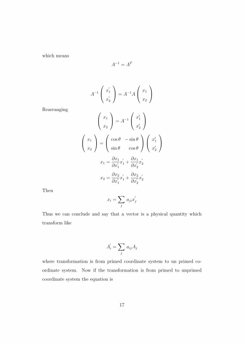
which means

A−1 = AT

A−1

x′1

x′2

= A−1A

x1

x2

Rearranging x1

x2

= A−1

x′1

x′2

x1

x2

=

cos θ − sin θ

sin θ cos θ

x′1

x′2

x1 =

∂x1∂x

′1

x′

1 +∂x1∂x

′2

x′

2

x2 =∂x2∂x

′1

x′

1 +∂x2∂x

′2

x′

2

Then

xi =∑j

ajix′

j

Thus we can conclude and say that a vector is a physical quantity which

transform like

A′

i =∑j

aijAj

where transformation is from primed coordinate system to un primed co-

ordinate system. Now if the transformation is from primed to unprimed

coordinate system the equation is

17

Ai =∑j

ajiA′

j

Both are definitions of a vector. This is very important and you must note

the indices.

2.1.3 Tensors

Mathematical expression for tensors

Consider the equation ~J = σ ~E. Here σ is a tensor. Let us derive the

expression for σ′

which is the equation in the primed coordinate system. In

matrix form the above equation is

Ji = σij Ej

Taking prime on both sides

J′

i = σ′

ij E′

j

But the component of J transform like J′i = aip Jp. Substituting

J′

i = σ′

ij E′

j = aip Jp

Writing the expression for J we get

J′

i = σ′

ij E′

j = aip Jp = aip σpqEq

18

Now using the inverse transformation equation for Eq,

σ′

ij E′

j = aip σpq ajqE′

j

Then we get

σ′

ij = aip ajqσpq

Thus we can see that a tensor of rank 2 will have 2 coefficients or the rank

of a tensor can be obtained from counting the number of coefficients.

Thus we can define tensors in general as

A′= A

tensor of rank zero or scalar

A′

i =∑j

aijAj

is tensor of rank one or vector and

A′

ij =∑p

∑q

aip ajqApq

is a tensor of rank 2 and if have 3 coefficients we will get tensor of rank 3 etc.

2.1.4 Summation Convention

In writing an expression such as a1x1 + a2x

2 + ..... + aNxN we can use the

short notationN∑j=1

ajxj. An even shorter notation is simply to write it as

19

ajxj, where we adopted the convention that whenever an index (subscript or

superscript)is repeated in a given term we are to sum over that index from

1 to N unless otherwise specified. This is called the “summation conven-

tion. Any index which is repeated in a given term ,so that the summation

convention applies , is called dummy index or umbral index. An index

occurring only once in a given term is called a free index. In tensor analy-

sis it is customary to adopt a summation convention and subsequent tensor

equations in a more compact form. As long as we are distinguishing between

contravariance and covariance, let us agree that when an index appears on

one side of an equation, once as a superscript and once as a subscript (except

for the coordinates where both are subscripts), we automatically sum over

that index.

20

Chapter 3

Quotient Rule

In tensor analysis it is often necessary to ascertain whether a given

quantity is tensor or not and if it is tensor we have to find its rank. The direct

method requires us to find out if the given quantity obeys the transformation

law or not. In practice this is troublesome and a similar test is provided by

a law known as Quotient law. Generally we can write,

K A = B

Here A and B are tensors of known rank and K is an unknown quantity. The

Quotient Rule gives the rank of K. For example

~L = I~ω

Here ~ω and ~L are known vectors, then Quotient Rule shows that I is a second

rank tensor. Similarly,

m~a = ~F

σ ~E = ~J

χ~E = ~P

all establish the second rank tensor of m,σ, χ. The well known Quotient

Rules are

21

KiAi = B

Kij Aj = Bi

Kij Ajk = Bik

KijklAij = Bkl

Kij Ak = Bijk

In each case A and B are known tensors of rank indicated by the

no. of indices and A is arbitrary where as in each case K is an unknown quan-

tity. We have to establish the transformation properties of K. The Quotient

Rule asserts that if the equation of interest holds in all Cartesian co-ordinate

system, K is a tensor of indicated rank. The importance in physical theory is

that the quotient rule establish the tensor nature of quantities. There is an

interesting idea that if we reconsider Newtons equations of motion m~a = ~F

on the basis of the quotient rule that, if the mass is a scalar and the force

a vector, then you can show that the acceleration ~a is a vector. In other

words, the vector character of the force as the driving term imposes its vec-

tor character on the acceleration, provided the scale factor m is scalar. This

will first make us think that it contradicts the idea given in the introduction.

But when we say m is scalar immediately we are considering that ~a and ~F

have the same directions which makes m scalar.

Now let us prove each equation and find the nature of K.

Proof for each rule

1.

K Ai = B

Proof

Taking prime on both sides

K′A

′

i = B′

Here A has one index and hence it is a vector. Using the transformation

22

equation for a vector

K′(∂x

′i

∂xj

)Aj = B

because B′

= B since it is a scalar. Now using the given rule RHS is

modified and we get

K′(∂x

′i

∂xj

)Aj = KAj

(K

′ ∂x′i

∂xj−K

)Aj = 0

Now Aj cannot be zero since it is a component and if it vanishes the law

itself does not exist. Hence the quantity within the bracket vanishes.

K =

(∂x

′i

∂xj

)K

′,

Here the transformation is with one coefficient and thus K is a first

rank tensor

2. The second quotient rule

K Aj = Bi

Proof

Now we will proceed as in the case of I law. Taking prime on both sides

K′A

′

j = B′

i

K′

(∂x

′j

∂xα

)Aα =

(∂x

′i

∂xl

)Bl

K′

(∂x

′j

∂xα

)Aα =

(∂x

′i

∂xl

)KAα(

K′ ∂x

′j

∂xα− ∂x

′i

∂xlK

)Aα = 0

K = K′

(∂x

′j

∂xα

∂xl∂x

′i

),

23

K is a second rank tensor

3. The third quotient rule

K Ajk = Bik

Proof

Taking prime

K′A

′

jk = B′

ik

K′

(∂x

′j

∂xα

∂x′

k

∂xβ

)Aαβ =

(∂x

′i

∂xγ

∂x′

k

∂xβ

)Bγβ

K′

(∂x

′j

∂xα

)Aαβ =

(∂x

′i

∂xγ

)KAαβ

K = K′

(∂x

′j

∂xα

∂xγ∂x

′i

),

K is a second rank tensor

4.

KAij = Bkl

Proof

Taking prime

K′A

′

ij = B′

kl

K′

(∂x

′i

∂xα

∂x′j

∂xβ

)Aαβ =

(∂x

′

k

∂xγ

∂x′

l

∂xν

)Bγν

K′

(∂x

′i

∂xα

∂x′j

∂xβ

)Aαβ =

(∂x

′

k

∂xγ

∂x′

l

∂xν

)KAαβ

K = K′

(∂x

′i

∂xα

∂x′j

∂xβ

∂xγ∂x

′k

∂xν∂x

′l

)K is a 4th rank tensor

5.

K Ak = Bijk

Proof

24

Taking prime

K′A

′

k = B′

ijk

K′(∂x

′

k

∂xl

)Al =

∂x′i

∂xα

∂x′j

∂xβ

∂x′

k

∂xlBαβl

K′(∂x

′

k

∂xl

)Al =

∂x′i

∂xα

∂x′j

∂xβ

∂x′

k

∂xlKAl

K = K′

(∂xα∂x

′i

∂xβ∂x

′j

)K is a second rank tensor. The quotient rule is a substitute for the

illegal division of tensors.

Problems

1. The double summation KijAiBj is invariant for any two vectors Ai and

Bj . Prove that Kij is a second-rank tensor.

2. The equation KijAjk = Bik holds for all orientations of the coordinate

system. If ~A and ~B are arbitrary second rank tensors show that K is a

second rank tensor.

25

Chapter 4

Non-Cartesian Tensors-Metric

Tensors

The metric tensor gij is a function which tells how to compute the distance

between any two points in a given space. Its components can be viewed

as multiplication factors which must be placed in front of the differential

displacements dxi in a generalized Pythagorean theorem. We can find the

metric tensor in spherical polar coordinates and cylindrical coordinates.

4.1 Spherical Polar Co-ordinate System

In Spherical Polar Co-ordinate System,

26

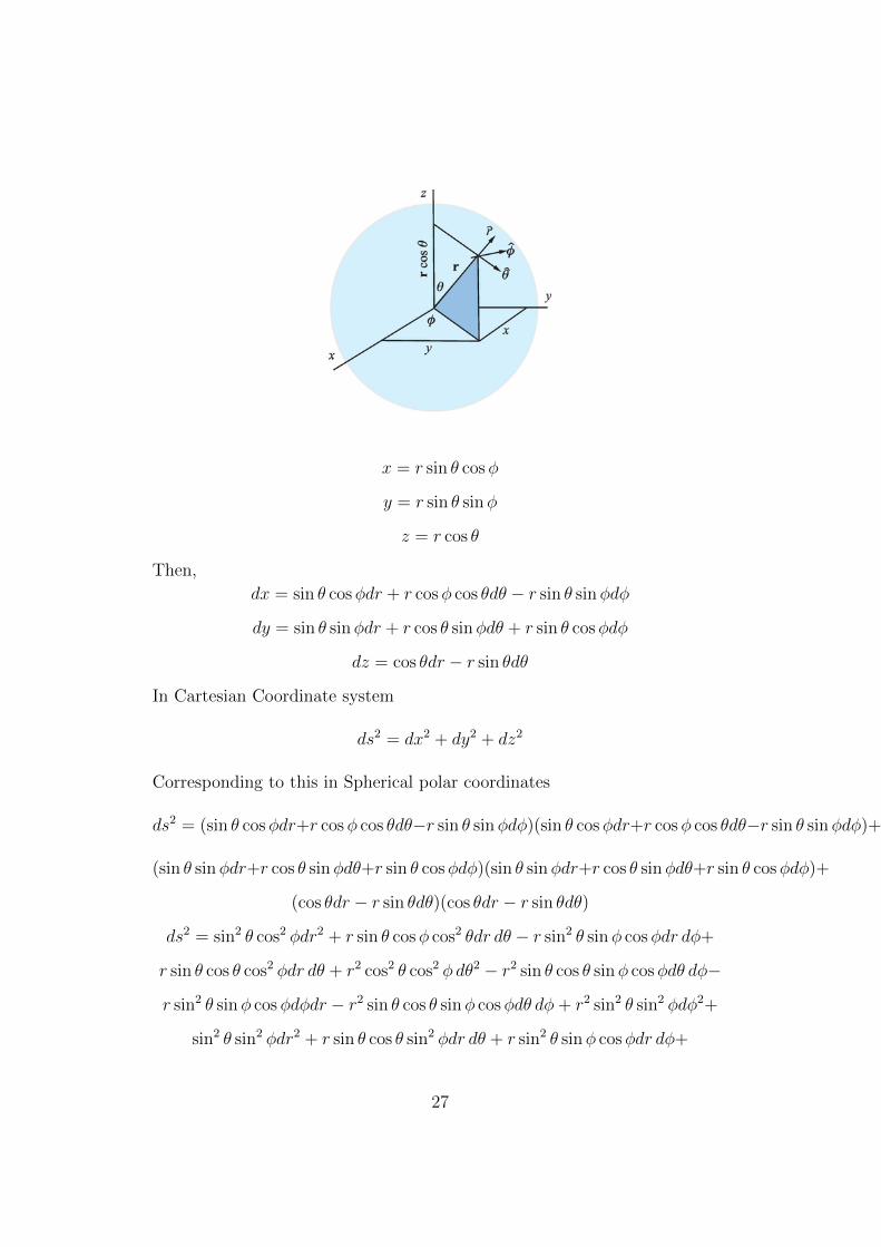
x = r sin θ cosφ

y = r sin θ sinφ

z = r cos θ

Then,

dx = sin θ cosφdr + r cosφ cos θdθ − r sin θ sinφdφ

dy = sin θ sinφdr + r cos θ sinφdθ + r sin θ cosφdφ

dz = cos θdr − r sin θdθ

In Cartesian Coordinate system

ds2 = dx2 + dy2 + dz2

Corresponding to this in Spherical polar coordinates

ds2 = (sin θ cosφdr+r cosφ cos θdθ−r sin θ sinφdφ)(sin θ cosφdr+r cosφ cos θdθ−r sin θ sinφdφ)+

(sin θ sinφdr+r cos θ sinφdθ+r sin θ cosφdφ)(sin θ sinφdr+r cos θ sinφdθ+r sin θ cosφdφ)+

(cos θdr − r sin θdθ)(cos θdr − r sin θdθ)

ds2 = sin2 θ cos2 φdr2 + r sin θ cosφ cos2 θdr dθ − r sin2 θ sinφ cosφdr dφ+

r sin θ cos θ cos2 φdr dθ + r2 cos2 θ cos2 φ dθ2 − r2 sin θ cos θ sinφ cosφdθ dφ−

r sin2 θ sinφ cosφdφdr − r2 sin θ cos θ sinφ cosφdθ dφ+ r2 sin2 θ sin2 φdφ2+

sin2 θ sin2 φdr2 + r sin θ cos θ sin2 φdr dθ + r sin2 θ sinφ cosφdr dφ+

27

r sin2 θ sinφ cosφdφ dr + r2 sin θ cos θ sinφ cosφdφ dθ + r2 sin2 θ cos2 θdφ2+

cos2 θdr2 − r sin θ cos θdr dθ − r sin θ cos θdr dθ + r2 sin2 θdθ2

= dr2 + r2dθ2 + r2 sin2 θdφ2 dx2

dy2

dz2

=

1 0 0

0 r2 0

0 0 r2 sin2 θ

dr2

dθ2

dφ2

ie,

gij =

1 0 0

0 r2 0

0 0 r2 sin2 θ

=

g11 g12 g13g21 g22 g23g31 g32 g33

ds2 = g11dr2 + g22dθ

2 + g33dφ2

For i 6= j , gij = 0

In general

= g11drdr+g12drdθ+g13drdφ+g21dθdr+g22dθdθ+g23dθdφ+g31dφdr+g32dφdθ+g33dφdφ

ds2 =∑i,j

gijdqidqj

Using sign convention

ds2 = gijdqidqj

Here ds2 is a scalar. We know from quotient rule that if

K Ai = B

K is a vector and hence gijdqj is a vector. Now if

K Ai = Bj

K is a second rank tensor and hence gij is a tensor of rank two. Thus gij is

called the metric tensor of rank two.

28

4.2 Cylindrical coordinate system

In Circular Cylindrical Co-ordinate System,

x = ρ cosφ

y = ρ sinφ

z = z

Differentiating and substituting we get

ds2 = dr2 + ρ2dφ2 + dz2 dx2

dy2

dz2

=

1 0 0

0 ρ2 0

0 0 1

dρ2

dφ2

dz2

Thus gij for cylindrical coordinate system can be found out.

Problem

In Minkowiski space we define x1 = x , x2 = y , x3 = z , and x0 = ct. This is

done so that the space time interval ds2 = dx20− dx21− dx22− dx23(c =velocity

of light). Show that the metric in Minkowiski space is

(gij) =

1 0 0 0

0 −1 0 0

0 0 −1 0

0 0 0 −1

29

Solution

x1 = x⇒ dx1 = dx

x2 = y ⇒ dx2 = dy

x3 = z ⇒ dx3 = dz

x0 = ct⇒ dx0 = c dt

Space time interval

ds2 = ds2 = dx20 − dx21 − dx22 − dx23

= c2dt2 − dx2 − dy2 − dz2

Then dx20dx21dx22dx23

=

1 0 0 0

0 −1 0 0

0 0 −1 0

0 0 0 −1

c2dt2

dx2

dy2

dz2

gij =

1 0 0 0

0 −1 0 0

0 0 −1 0

0 0 0 −1

30

Chapter 5

Algebraic Operation of Tensors

5.0.1 Definition of Contravariant and Co variant vec-

tor

Contravariant vector

We’ve

x′i =∑j

aijxj

or in general

Ai′=∑j

∂xi′

∂xjAj

Any vector whose components transform like this expression is defined as

Contravariant vector Here we have used superscript to denote the compo-

nent. This is to differentiate it from another type of vector which we will

shortly define. Examples are displacement, velocity, acceleration etc

31

5.0.2 Exercises

1. If xi be the co-ordinate of a point in 2-dimensional space. Show that

dxi are component of a contravariant tensor?

Soln: Earlier we have studied transformation from X to X’ coordinates.

There we have

x′

1 = x1 cos θ + x2 sin θ

x′

2 = −x1 sin θ + x2 cos θ

Writing in the superscript form we have x1′

is a function of x1 and x2

xi′= xi

′ (x1, x2

)Using the method of partial differential

dxi′=∂xi

′

∂x1dx1 +

∂xi′

∂x2dx2

dxi′=∑j

∂xi′

∂xjdxj

It is the transformation equation for a contravariant vector

2. Show that the velocity of a fluid at any point is component of a con-

travariant vector?

Soln:

Velocity is rate of change of displacement. Hence we can take the

equation for displacement from the previous problem.

dxi′=∂xi

′

∂x1dx1 +

∂xi′

∂x2dx2

dxi′

dt=∂xi

′

∂x1dx1

dt+∂xi

′

∂x2dx2

dt

dxi′

dt=∑j

∂xi′

∂xjdxj

dt

V i′ =∑j

dxi′

dxjV j

32

where V i′ and V j are the components of velocity.

It is a contravariant vector.

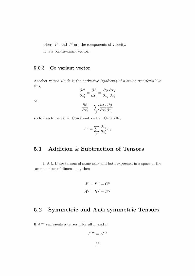
5.0.3 Co variant vector

Another vector which is the derivative (gradient) of a scalar transform like

this,∂φ′

∂x′i=∂φ

∂x′i=

∂φ

∂xj

∂xj∂x′i

or,∂φ

∂x′i=∑j

∂xj∂x′i

∂φ

∂xj

such a vector is called Co-variant vector. Generally,

Ai′=∑j

∂xj∂x′i

Aj

5.1 Addition & Subtraction of Tensors

If A & B are tensors of same rank and both expressed in a space of the

same number of dimensions, then

Aij +Bij = Cij

Aij −Bij = Dij

5.2 Symmetric and Anti symmetric Tensors

If Amn represents a tensor,if for all m and n

Amn = Anm

33

we call it as a symmetric tensor and if on other hand

Amn = −Anm

the tensor is anti symmetric.

We can write,

Amn =1

2Amn+

1

2Amn =

(1

2Amn +

1

2Anm

)+

(1

2Amn − 1

2Anm

)= Bmn+Cmn

Interchanging the indices we can show that

Bnm = Bmn

which is symmetric

Cnm = −Cmn

which is antisymmetric. So Amn can be represented as a combination of sym-

metric and anti symmetric parts.

5.3 Problems

1. If a physical quantity has no component in one coordinate system, then

show that it does not have a component in other coordinate systems

Answer

We have transformation equations like

Aij′=∂x′i∂xk

∂x′j∂xl

Akl

V i′ =∑j

dxi′

dxjV j

Vθ =dθ

dyVy

These equations show that if a physical quantity exist in one coordinate

system it exists in other coordinate system also. Hence if it vanishes in

a system it vanishes in other systems also.

34

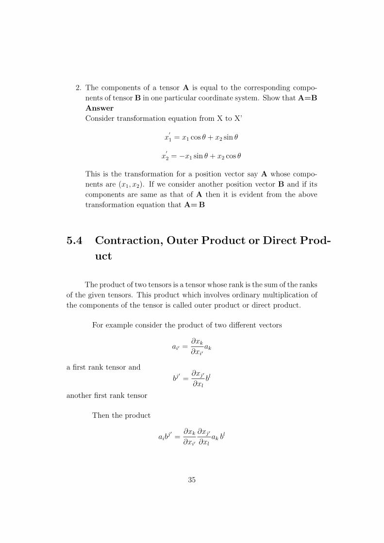
2. The components of a tensor A is equal to the corresponding compo-

nents of tensor B in one particular coordinate system. Show that A=B

Answer

Consider transformation equation from X to X’

x′

1 = x1 cos θ + x2 sin θ

x′

2 = −x1 sin θ + x2 cos θ

This is the transformation for a position vector say A whose compo-

nents are (x1, x2). If we consider another position vector B and if its

components are same as that of A then it is evident from the above

transformation equation that A= B

5.4 Contraction, Outer Product or Direct Prod-

uct

The product of two tensors is a tensor whose rank is the sum of the ranks

of the given tensors. This product which involves ordinary multiplication of

the components of the tensor is called outer product or direct product.

For example consider the product of two different vectors

ai′ =∂xk∂xi′

ak

a first rank tensor and

bj′=∂xj′

∂xlbl

another first rank tensor

Then the product

aibj′ =

∂xk∂xi′

∂xj′

∂xlak b

l

35

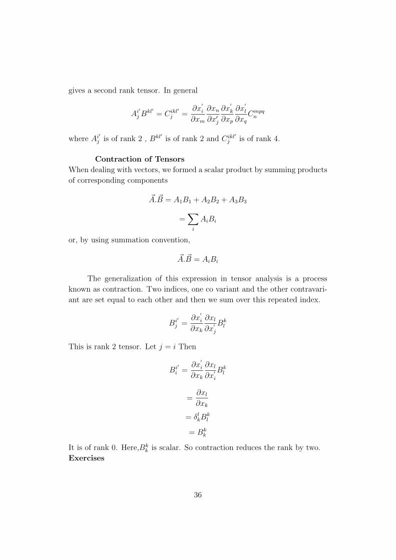
gives a second rank tensor. In general

Ai′

jBkl′ = Cikl′

j =∂x

′i

∂xm

∂xn∂x′j

∂x′

k

∂xp

∂x′

l

∂xqCmpqn

where Ai′j is of rank 2 , Bkl′ is of rank 2 and Cikl′

j is of rank 4.

Contraction of Tensors

When dealing with vectors, we formed a scalar product by summing products

of corresponding components

~A. ~B = A1B1 + A2B2 + A3B3

=∑i

AiBi

or, by using summation convention,

~A. ~B = AiBi

The generalization of this expression in tensor analysis is a process

known as contraction. Two indices, one co variant and the other contravari-

ant are set equal to each other and then we sum over this repeated index.

Bi′

j =∂x

′i

∂xk

∂xl∂x

′j

Bkl

This is rank 2 tensor. Let j = i Then

Bi′

i =∂x

′i

∂xk

∂xl∂x

′i

Bkl

=∂xl∂xk

= δlkBkl

= Bkk

It is of rank 0. Here,Bkk is scalar. So contraction reduces the rank by two.

Exercises

36

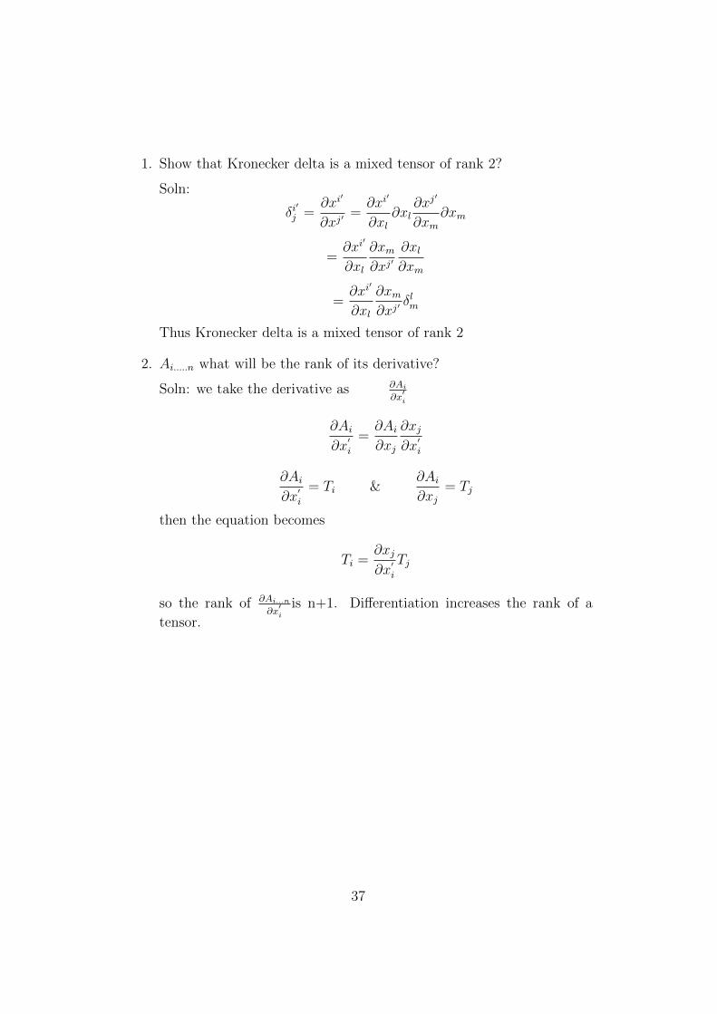
1. Show that Kronecker delta is a mixed tensor of rank 2?

Soln:

δi′

j =∂xi

′

∂xj′=∂xi

′

∂xl∂xl

∂xj′

∂xm∂xm

=∂xi

′

∂xl

∂xm∂xj′

∂xl∂xm

=∂xi

′

∂xl

∂xm∂xj′

δlm

Thus Kronecker delta is a mixed tensor of rank 2

2. Ai.....n what will be the rank of its derivative?

Soln: we take the derivative as ∂Ai

∂x′i

∂Ai∂x

′i

=∂Ai∂xj

∂xj∂x

′i

∂Ai∂x

′i

= Ti &∂Ai∂xj

= Tj

then the equation becomes

Ti =∂xj∂x

′i

Tj

so the rank of ∂Ai...n

∂x′i

is n+1. Differentiation increases the rank of a

tensor.

37

Chapter 6

Pseudo Scalars and Pseudo

Vectors and Pseudo Tensors

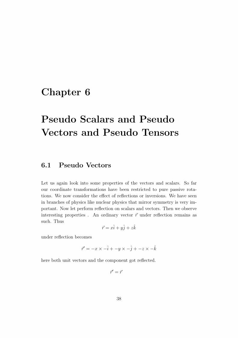
6.1 Pseudo Vectors

Let us again look into some properties of the vectors and scalars. So far

our coordinate transformations have been restricted to pure passive rota-

tions. We now consider the effect of reflections or inversions. We have seen

in branches of physics like nuclear physics that mirror symmetry is very im-

portant. Now let perform reflection on scalars and vectors. Then we observe

interesting properties . An ordinary vector ~r under reflection remains as

such. Thus

~r = xi+ yj + zk

under reflection becomes

~r′ = −x×−i+−y ×−j +−z ×−k

here both unit vectors and the component got reflected.

~r′ = ~r

38

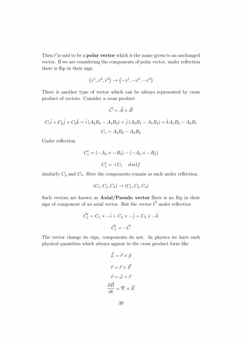
Then ~r is said to be a polar vector which is the name given to an unchanged

vector. If we are considering the components of polar vector, under reflection

there is flip in their sign.(x1, x2, x3

)→(−x1,−x2,−x3

)There is another type of vector which can be always represented by cross

product of vectors. Consider a cross product

~C = ~A× ~B

C1i+ C2j + C3k = i (A2B3 − A3B2) + j (A3B1 − A1B3) + kA1B2 − A2B1

C1 = A2B3 − A3B2

Under reflection

C ′1 = (−A2 ×−B3)− (−A3 ×−B2)

C ′1 = +C1 itself

similarly C2 and C3. Here the components remain as such under reflection.

(C1, C2, C3)→ (C1, C2, C3)

Such vectors are known as Axial/Pseudo vector fhere is no flip in their

sign of component of an axial vector. But the vector ~C under reflection

~C ′1 = C1 ×−i+ C2 ×−j + C3 ×−k

~C ′1 = −~C

The vector change its sign, components do not. In physics we have such

physical quantities which always appear in the cross product form like

~L = ~r × ~p

~τ = ~r × ~F

~v = ~ω × ~r

∂ ~B

∂t= ∇× ~E

39

Here ~L ,~τ , ω, ~B are pseudo vectors.

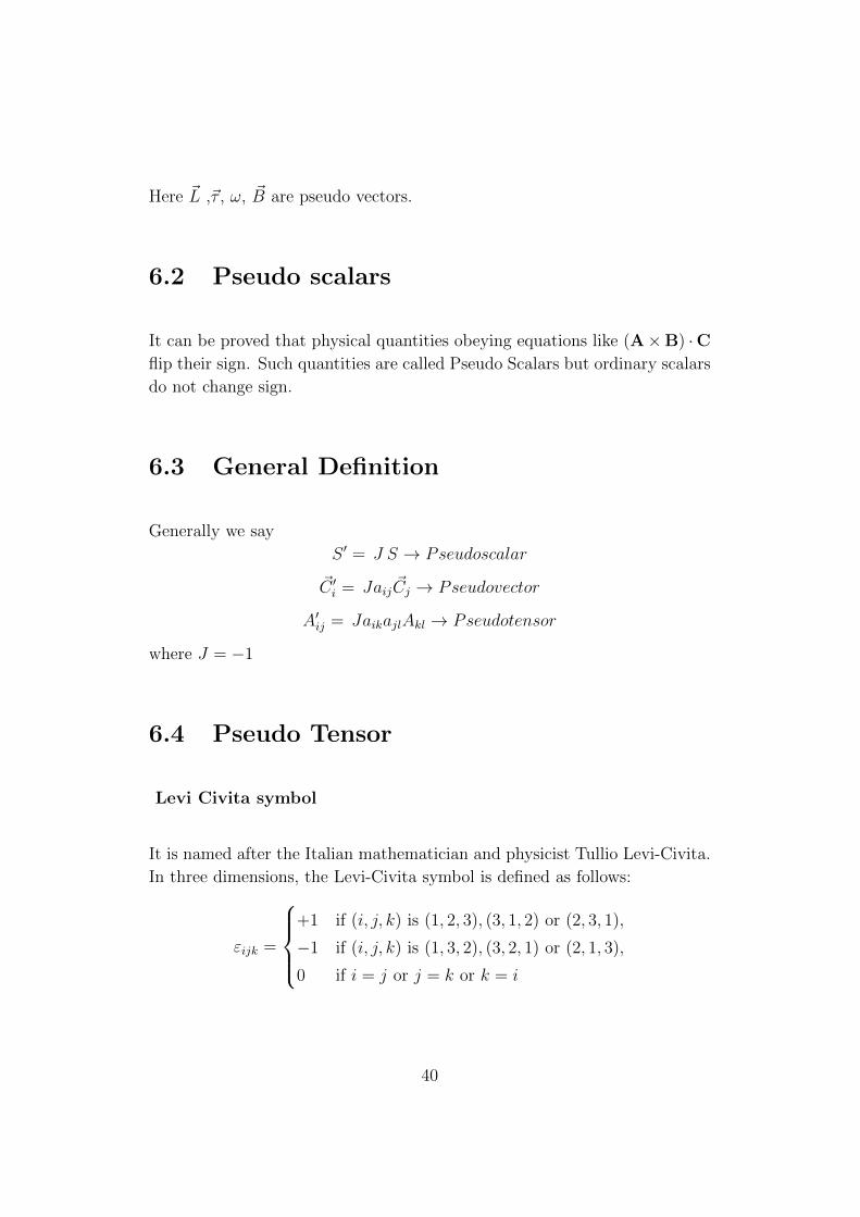
6.2 Pseudo scalars

It can be proved that physical quantities obeying equations like (A×B) ·Cflip their sign. Such quantities are called Pseudo Scalars but ordinary scalars

do not change sign.

6.3 General Definition

Generally we say

S ′ = J S → Pseudoscalar

~C ′i = Jaij ~Cj → Pseudovector

A′ij = JaikajlAkl → Pseudotensor

where J = −1

6.4 Pseudo Tensor

Levi Civita symbol

It is named after the Italian mathematician and physicist Tullio Levi-Civita.

In three dimensions, the Levi-Civita symbol is defined as follows:

εijk =

+1 if (i, j, k) is (1, 2, 3), (3, 1, 2) or (2, 3, 1),

−1 if (i, j, k) is (1, 3, 2), (3, 2, 1) or (2, 1, 3),

0 if i = j or j = k or k = i

40

The Levi-Civita symbol is not a physical quantity but it is always associated

with some physical quantity. To establish this consider cross product of two

vectors ~A and ~B~C = ~A× ~B

=

∣∣∣∣∣∣∣i j k

A1 A2 A3

B1 B2 B3

∣∣∣∣∣∣∣C1 = A2B3 − A3B2

C2 = A3B1 − A1B3

C3 = A1B2 − A2B1

The three equation can be generalized as

Ci = εijkAjBk

Putting i = 1, 2, 3 etc. we can deduce C1, C2, C3

Putting i=1

C1 =3∑

j,k=1

ε1jkAjBk

=∑k

[ε11kA1Bk + ε12kA2Bk + ε13kA3Bk]

= A2B3 − A3B2

Similarly putting i=2, i=3 we can deduce C2 and C3.

Now we will show that Levi-Civita[LC] symbol εijk is a pseudo tensor?

Proof:If Levi Civita symbol is a pseudo tensor then its transformation equa-

tion is

ε′ijk = |a| aipajqakrεpqr

For an ordinary vector

x′i = aijxj

For rotation this is (x

′1

x′2

)=

(cos θ sin θ

− sin θ cos θ

)(x1x2

)

41

Which can be written as

x′i = |A|aijxj

where determinant is 1, but in the case of pseudo vectors it will be −1 Then

for i = 1, j = 2, k = 3

1 = |a| a1pa2qa3rεpqr

= |a|3∑

pqr=1

a1pa2qa3rεpqr

Then∑pqr

a1pa2qa3rεpqr =∑qr

[a11a2qa3rε1qr + a12a2qa3rε2qr + a13a2qa3rε3qr]

Summing over q and r

= a12a23a31ε231+a13a22a31ε321+a11a23a32ε132+a13a21a32ε312+a11a22a33ε123+a12a21a33ε213

= a12a23a31 − a13a22a31 − a11a23a32 + a13a21a32 + a11a22a33 − a12a21a33

= a11 (a22a33 − a23a32) + a12 (a23a31 − a21a33) + a13 (a21a32 − a22a31)

=

∣∣∣∣∣∣a11 a12 a13a21 a22 a23a31 a32 a33

∣∣∣∣∣∣so,

1 = |a| |a| = 1

since by definition of pseudo tensors

|a| = −1

ε′ijk = RHS

which shows that LC satisfies the definition of a pseudo tensor.

Solved Problems

1. Use the antisymmetry of εijk to show that ~A.(~A× ~B

)= 0

42

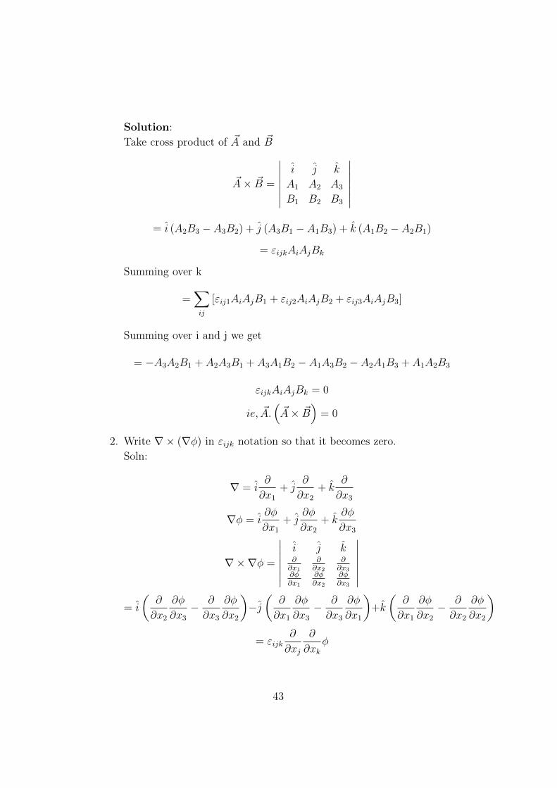
Solution:

Take cross product of ~A and ~B

~A× ~B =

∣∣∣∣∣∣∣i j k

A1 A2 A3

B1 B2 B3

∣∣∣∣∣∣∣= i (A2B3 − A3B2) + j (A3B1 − A1B3) + k (A1B2 − A2B1)

= εijkAiAjBk

Summing over k

=∑ij

[εij1AiAjB1 + εij2AiAjB2 + εij3AiAjB3]

Summing over i and j we get

= −A3A2B1 + A2A3B1 + A3A1B2 − A1A3B2 − A2A1B3 + A1A2B3

εijkAiAjBk = 0

ie, ~A.(~A× ~B

)= 0

2. Write ∇× (∇φ) in εijk notation so that it becomes zero.

Soln:

∇ = i∂

∂x1+ j

∂

∂x2+ k

∂

∂x3

∇φ = i∂φ

∂x1+ j

∂φ

∂x2+ k

∂φ

∂x3

∇×∇φ =

∣∣∣∣∣∣∣i j k∂∂x1

∂∂x2

∂∂x3

∂φ∂x1

∂φ∂x2

∂φ∂x3

∣∣∣∣∣∣∣= i

(∂

∂x2

∂φ

∂x3− ∂

∂x3

∂φ

∂x2

)−j(

∂

∂x1

∂φ

∂x3− ∂

∂x3

∂φ

∂x1

)+k

(∂

∂x1

∂φ

∂x2− ∂

∂x2

∂φ

∂x2

)= εijk

∂

∂xj

∂

∂xkφ

43

3∑ijk=1

εijk∂

∂xj

∂

∂xkφ =

∑jk

ε1jk∂

∂xj

∂

∂xkφ+ ε2jk

∂

∂xj

∂

∂xkφ+ ε3jk

∂

∂xj

∂

∂xkφ

Expanding we get

= 0

3. Show that δii = 3

4. Show that δijεijk = 0

5. Show that εipqεjpq = 2δij

6. Show that εijkεijk = 6

44