267
Notes on Microeconomic Theory Nolan H. Miller August 18, 2006
| Date post: | 27-Oct-2014 |
| Category: |
Documents |
| Upload: | alfascorpion |
| View: | 669 times |
| Download: | 0 times |

Notes on Microeconomic Theory
Nolan H. Miller
August 18, 2006

Contents
1 The Economic Approach 1
2 Consumer Theory Basics 5
2.1 Commodities and Budget Sets . . . . . . . . . . . . . . . . . . . . . . . . . . . . . . . 5
2.2 Demand Functions . . . . . . . . . . . . . . . . . . . . . . . . . . . . . . . . . . . . . 8
2.3 Three Restrictions on Consumer Choices . . . . . . . . . . . . . . . . . . . . . . . . . 9
2.4 A First Analysis of Consumer Choices . . . . . . . . . . . . . . . . . . . . . . . . . . 10
2.4.1 Comparative Statics . . . . . . . . . . . . . . . . . . . . . . . . . . . . . . . . 11
2.5 Requirement 1 Revisited: Walras’ Law . . . . . . . . . . . . . . . . . . . . . . . . . . 11
2.5.1 What’s the Funny Equals Sign All About? . . . . . . . . . . . . . . . . . . . . 12
2.5.2 Back to Walras’ Law: Choice Response to a Change in Wealth . . . . . . . . 13
2.5.3 Testable Implications . . . . . . . . . . . . . . . . . . . . . . . . . . . . . . . 14
2.5.4 Summary: How Did We Get Where We Are? . . . . . . . . . . . . . . . . . . 15
2.5.5 Walras’ Law: Choice Response to a Change in Price . . . . . . . . . . . . . . 15
2.5.6 Comparative Statics in Terms of Elasticities . . . . . . . . . . . . . . . . . . . 16
2.5.7 Why Bother? . . . . . . . . . . . . . . . . . . . . . . . . . . . . . . . . . . . . 17
2.5.8 Walras’ Law and Changes in Wealth: Elasticity Form . . . . . . . . . . . . . 18
2.6 Requirement 2 Revisited: Demand is Homogeneous of Degree Zero. . . . . . . . . . . 18
2.6.1 Comparative Statics of Homogeneity of Degree Zero . . . . . . . . . . . . . . 19
2.6.2 A Mathematical Aside ... . . . . . . . . . . . . . . . . . . . . . . . . . . . . . 21
2.7 Requirement 3 Revisited: The Weak Axiom of Revealed Preference . . . . . . . . . . 22
2.7.1 Compensated Changes and the Slutsky Equation . . . . . . . . . . . . . . . . 23
2.7.2 Other Properties of the Substitution Matrix . . . . . . . . . . . . . . . . . . . 27
i

Nolan Miller Notes on Microeconomic Theory ver: Aug. 2006
3 The Traditional Approach to Consumer Theory 29
3.1 Basics of Preference Relations . . . . . . . . . . . . . . . . . . . . . . . . . . . . . . . 30
3.2 From Preferences to Utility . . . . . . . . . . . . . . . . . . . . . . . . . . . . . . . . 35
3.2.1 Utility is an Ordinal Concept . . . . . . . . . . . . . . . . . . . . . . . . . . . 36
3.2.2 Some Basic Properties of Utility Functions . . . . . . . . . . . . . . . . . . . 37
3.3 The Utility Maximization Problem (UMP) . . . . . . . . . . . . . . . . . . . . . . . . 42
3.3.1 Walrasian Demand Functions and Their Properties . . . . . . . . . . . . . . . 47
3.3.2 The Lagrange Multiplier . . . . . . . . . . . . . . . . . . . . . . . . . . . . . . 49
3.3.3 The Indirect Utility Function and Its Properties . . . . . . . . . . . . . . . . 50
3.3.4 Roy’s Identity . . . . . . . . . . . . . . . . . . . . . . . . . . . . . . . . . . . . 52
3.3.5 The Indirect Utility Function and Welfare Evaluation . . . . . . . . . . . . . 54
3.4 The Expenditure Minimization Problem (EMP) . . . . . . . . . . . . . . . . . . . . . 55
3.4.1 A First Note on Duality . . . . . . . . . . . . . . . . . . . . . . . . . . . . . . 57
3.4.2 Properties of the Hicksian Demand Functions and Expenditure Function . . . 59
3.4.3 The Relationship Between the Expenditure Function and Hicksian Demand . 62
3.4.4 The Slutsky Equation . . . . . . . . . . . . . . . . . . . . . . . . . . . . . . . 65
3.4.5 Graphical Relationship of the Walrasian and Hicksian Demand Functions . . 67
3.4.6 The EMP and the UMP: Summary of Relationships . . . . . . . . . . . . . . 71
3.4.7 Welfare Evaluation . . . . . . . . . . . . . . . . . . . . . . . . . . . . . . . . . 72
3.4.8 Bringing It All Together . . . . . . . . . . . . . . . . . . . . . . . . . . . . . . 78
3.4.9 Welfare Evaluation for an Arbitrary Price Change . . . . . . . . . . . . . . . 83
4 Topics in Consumer Theory 87
4.1 Homothetic and Quasilinear Utility Functions . . . . . . . . . . . . . . . . . . . . . . 87
4.2 Aggregation . . . . . . . . . . . . . . . . . . . . . . . . . . . . . . . . . . . . . . . . . 89
4.2.1 The Gorman Form . . . . . . . . . . . . . . . . . . . . . . . . . . . . . . . . . 90
4.2.2 Aggregate Demand and Aggregate Wealth . . . . . . . . . . . . . . . . . . . . 92
4.2.3 Does individual WARP imply aggregate WARP? . . . . . . . . . . . . . . . . 94
4.2.4 Representative Consumers . . . . . . . . . . . . . . . . . . . . . . . . . . . . . 96
4.3 The Composite Commodity Theorem . . . . . . . . . . . . . . . . . . . . . . . . . . . 98
4.4 So Were They Just Lying to Me When I Studied Intermediate Micro? . . . . . . . . 99
4.5 Consumption With Endowments . . . . . . . . . . . . . . . . . . . . . . . . . . . . . 101
ii

Nolan Miller Notes on Microeconomic Theory ver: Aug. 2006
4.5.1 The Labor-Leisure Choice . . . . . . . . . . . . . . . . . . . . . . . . . . . . . 104
4.5.2 Consumption with Endowments: A Simple Separation Theorem . . . . . . . . 106
4.6 Consumption Over Time . . . . . . . . . . . . . . . . . . . . . . . . . . . . . . . . . . 110
4.6.1 Discounting and Present Value . . . . . . . . . . . . . . . . . . . . . . . . . . 111
4.6.2 The Two-Period Model . . . . . . . . . . . . . . . . . . . . . . . . . . . . . . 112
4.6.3 The Many-Period Model and Time Preference . . . . . . . . . . . . . . . . . . 115
4.6.4 The Fisher Separation Theorem . . . . . . . . . . . . . . . . . . . . . . . . . . 118
5 Producer Theory 121
5.1 Production Sets . . . . . . . . . . . . . . . . . . . . . . . . . . . . . . . . . . . . . . . 122
5.1.1 Properties of Production Sets . . . . . . . . . . . . . . . . . . . . . . . . . . . 123
5.1.2 Profit Maximization with Production Sets . . . . . . . . . . . . . . . . . . . . 127
5.1.3 Properties of the Net Supply and Profit Functions . . . . . . . . . . . . . . . 129
5.1.4 A Note on Recoverability . . . . . . . . . . . . . . . . . . . . . . . . . . . . . 132
5.2 Production with a Single Output . . . . . . . . . . . . . . . . . . . . . . . . . . . . . 133
5.2.1 Profit Maximization with a Single Output . . . . . . . . . . . . . . . . . . . . 134
5.3 Cost Minimization . . . . . . . . . . . . . . . . . . . . . . . . . . . . . . . . . . . . . 136
5.3.1 Properties of the Conditional Factor Demand and Cost Functions . . . . . . . 138
5.3.2 Return to Recoverability . . . . . . . . . . . . . . . . . . . . . . . . . . . . . . 139
5.4 Why Do You Keep Doing This to Me? . . . . . . . . . . . . . . . . . . . . . . . . . . 140
5.5 The Geometry of Cost Functions . . . . . . . . . . . . . . . . . . . . . . . . . . . . . 141
5.6 Aggregation of Supply . . . . . . . . . . . . . . . . . . . . . . . . . . . . . . . . . . . 142
5.7 A First Crack at the Welfare Theorems . . . . . . . . . . . . . . . . . . . . . . . . . 143
5.8 Constant Returns Technologies . . . . . . . . . . . . . . . . . . . . . . . . . . . . . . 144
5.9 Household Production Models . . . . . . . . . . . . . . . . . . . . . . . . . . . . . . . 148
5.9.1 Agricultural Household Models with Complete Markets . . . . . . . . . . . . 149
6 Choice Under Uncertainty 158
6.1 Lotteries . . . . . . . . . . . . . . . . . . . . . . . . . . . . . . . . . . . . . . . . . . . 160
6.1.1 Preferences Over Lotteries . . . . . . . . . . . . . . . . . . . . . . . . . . . . . 161
6.1.2 The Expected Utility Theorem . . . . . . . . . . . . . . . . . . . . . . . . . . 164
6.1.3 Constructing a vNM utility function . . . . . . . . . . . . . . . . . . . . . . . 167
6.2 Utility for Money and Risk Aversion . . . . . . . . . . . . . . . . . . . . . . . . . . . 168
iii

Nolan Miller Notes on Microeconomic Theory ver: Aug. 2006
6.2.1 Measuring Risk Aversion: Coefficients of Absolute and Relative Risk Aversion173
6.2.2 Comparing Risk Aversion . . . . . . . . . . . . . . . . . . . . . . . . . . . . . 174
6.2.3 A Note on Comparing Distributions: Stochastic Dominance . . . . . . . . . . 176
6.3 Some Applications . . . . . . . . . . . . . . . . . . . . . . . . . . . . . . . . . . . . . 178
6.3.1 Insurance . . . . . . . . . . . . . . . . . . . . . . . . . . . . . . . . . . . . . . 178
6.3.2 Investing in a Risky Asset: The Portfolio Problem . . . . . . . . . . . . . . . 180
6.4 Ex Ante vs. Ex Post Risk Management . . . . . . . . . . . . . . . . . . . . . . . . . 182
7 Competitive Markets and Partial Equilibrium Analysis 185
7.1 Competitive Equilibrium . . . . . . . . . . . . . . . . . . . . . . . . . . . . . . . . . . 186
7.1.1 Allocations and Pareto Optimality . . . . . . . . . . . . . . . . . . . . . . . . 186
7.1.2 Competitive Equilibria . . . . . . . . . . . . . . . . . . . . . . . . . . . . . . . 188
7.2 Partial Equilibrium Analysis . . . . . . . . . . . . . . . . . . . . . . . . . . . . . . . 191
7.2.1 Set-Up of the Quasilinear Model . . . . . . . . . . . . . . . . . . . . . . . . . 191
7.2.2 Analysis of the Quasilinear Model . . . . . . . . . . . . . . . . . . . . . . . . 192
7.2.3 A Bit on Social Cost and Benefit . . . . . . . . . . . . . . . . . . . . . . . . . 195
7.2.4 Comparative Statics . . . . . . . . . . . . . . . . . . . . . . . . . . . . . . . . 195
7.3 The Fundamental Welfare Theorems . . . . . . . . . . . . . . . . . . . . . . . . . . . 198
7.3.1 Welfare Analysis and Partial Equilibrium . . . . . . . . . . . . . . . . . . . . 201
7.4 Entry and Long-Run Competitive Equilibrium . . . . . . . . . . . . . . . . . . . . . 205
7.4.1 Long-Run Competitive Equilibrium . . . . . . . . . . . . . . . . . . . . . . . 206
7.4.2 Final Comments on Partial Equilibrium . . . . . . . . . . . . . . . . . . . . . 209
8 Externalities and Public Goods 211
8.1 What is an Externality? . . . . . . . . . . . . . . . . . . . . . . . . . . . . . . . . . . 211
8.2 Bilateral Externalities . . . . . . . . . . . . . . . . . . . . . . . . . . . . . . . . . . . 213
8.2.1 Traditional Solutions to the Externality Problem . . . . . . . . . . . . . . . . 217
8.2.2 Bargaining and Enforceable Property Rights: Coase’s Theorem . . . . . . . . 219
8.2.3 Externalities and Missing Markets . . . . . . . . . . . . . . . . . . . . . . . . 221
8.3 Public Goods and Pure Public Goods . . . . . . . . . . . . . . . . . . . . . . . . . . 222
8.3.1 Pure Public Goods . . . . . . . . . . . . . . . . . . . . . . . . . . . . . . . . . 223
8.3.2 Remedies for the Free-Rider Problem . . . . . . . . . . . . . . . . . . . . . . . 227
8.3.3 Club Goods . . . . . . . . . . . . . . . . . . . . . . . . . . . . . . . . . . . . . 229
iv

Nolan Miller Notes on Microeconomic Theory ver: Aug. 2006
8.4 Common-Pool Resources . . . . . . . . . . . . . . . . . . . . . . . . . . . . . . . . . . 229
9 Monopoly 233
9.1 Simple Monopoly Pricing . . . . . . . . . . . . . . . . . . . . . . . . . . . . . . . . . 233
9.2 Non-Simple Pricing . . . . . . . . . . . . . . . . . . . . . . . . . . . . . . . . . . . . . 236
9.2.1 Non-Linear Pricing . . . . . . . . . . . . . . . . . . . . . . . . . . . . . . . . . 237
9.2.2 Two-Part Tariffs . . . . . . . . . . . . . . . . . . . . . . . . . . . . . . . . . . 239
9.3 Price Discrimination . . . . . . . . . . . . . . . . . . . . . . . . . . . . . . . . . . . . 241
9.3.1 First-Degree Price Discrimination . . . . . . . . . . . . . . . . . . . . . . . . . 241
9.3.2 Second-Degree Price Discrimination . . . . . . . . . . . . . . . . . . . . . . . 243
9.3.3 Third-Degree Price Discrimination . . . . . . . . . . . . . . . . . . . . . . . . 247
9.4 Natural Monopoly and Ramsey Pricing . . . . . . . . . . . . . . . . . . . . . . . . . 249
9.4.1 Regulation and Incentives . . . . . . . . . . . . . . . . . . . . . . . . . . . . . 251
9.5 Further Topics in Monopoly Pricing . . . . . . . . . . . . . . . . . . . . . . . . . . . 252
9.5.1 Multi-Product Monopoly . . . . . . . . . . . . . . . . . . . . . . . . . . . . . 252
9.5.2 Intertemporal Pricing . . . . . . . . . . . . . . . . . . . . . . . . . . . . . . . 255
9.5.3 Durable Goods Monopoly . . . . . . . . . . . . . . . . . . . . . . . . . . . . . 256
v

Nolan Miller Notes on Microeconomic Theory ver: Aug. 2006
These notes are intended for use in courses in microeconomic theory taught at Harvard Univer-
sity. Consequently, much of the structure is inherited from the required text for the course, which
is currently Mas-Colell, Whinston, and Green’s Microeconomic Theory (referred to as MWG in
these notes). They also draw on material contained in Silberberg’s The Structure of Economics, as
well as additional sources. They are not intended to stand alone or in any way replace the texts.
In the early drafts of this document, there will undoubtedly be mistakes. I welcome comments
from students regarding typographical errors, just-plain errors, or other comments on how these
notes can be made more helpful.
I thank Chris Avery, Lori Snyder, and Ben Sommers for helping clarify these notes and finding
many errors.
vi

Chapter 1
The Economic Approach
Economics is a social science.1 Social sciences are concerned with the study of human behavior.
If you asked the next person you meet while walking down the street what defines the difference
between economics and other social sciences, such as political science or sociology, that person
would most likely say that economics studies money, interest rates, prices, profits, and the like,
while political science considers politicians, elections, etc., and sociology studies the behavior of
groups of people. However, while there is certainly some truth to this statement, the things that
can be fairly called economics are not so much defined by a subject matter as they are united by
a common approach to problems. In fact, economists have written on topics spanning human
behavior, from traditional studies of firm and consumer behavior, interest rates, inflation and
unemployment to less traditional topics such as social choice, voting, marriage, and family.
The feature that unites these studies is a common approach to problems, which has become
known as the “marginalist” or “neoclassical” approach. In a nutshell, the marginalist approach
consists of four principles:
1. Economic actors have preferences over allocations of the world’s resources. These preferences
remain stable, at least over the period of time under study.2
2. There are constraints placed on the allocations that a person can achieve by such things as
wealth, physical availability, and social/political institutions.
3. Given the limits in (2), people choose the allocation that they most prefer.
1See Silberberg’s Structure of Economics for a more extended discussion along these lines.2Often preferences that change can be captured by adding another attribute to the description of an allocation.
1

Nolan Miller Notes on Microeconomic Theory: Chapter 1 ver: Aug. 2006
4. Changes in the allocations people choose are due to changes in the limits on available resources
in (2).
The marginalist approach to problems allows the economist to derive predictions about behavior
which can then, in principle, be tested against real world data using statistical (econometric)
techniques. For example, consider the problem of what I should buy when I go to the grocery
store. The grocery store is filled with different types of food, some of which I like more and some of
which I like less. Principle (1) says that the trade-offs I am willing to make among the various items
in the store are well-defined and stable, at least over the course of a few months. An allocation is
all of the stuff that I decide to buy. The constraints (2) put on the allocations I can buy include
the stock of the items in the store (I can’t buy more bananas than they have) and the money in
my pocket (I can’t buy bananas I can’t afford). Principle (3) says that given my preferences, the
amount of money in my pocket and the stock of items in the store, I choose the shopping cart full
of stuff that I most prefer. That is, when I walk out of the store, there is no other shopping cart
full of stuff that I could have purchased that I would have preferred to the one I did purchase.
Principle (4) says that if next week I buy a different cart full of groceries, it is because either I have
less money, something I bought last week wasn’t available this week, or something I bought this
week wasn’t available last week.
There are two natural objections to the story I told in the last paragraph, both of which point
toward why doing economics isn’t a trivial exercise. First, it is not necessarily the case that my
preferences remain stable. In particular, it is reasonable to think that my preferences this week
will depend on what I purchased last week. For example, if I purchased chocolate chip cookies
last week, this may make me less likely to purchase them this week and more likely to purchase
some other sort of cookie. Thus, preferences may not be stable over the time period we are
studying. Economists deal with this problem in two ways. The first is by ignoring it. Although
widely applied, this is not the best way to address the problem. However, there are circumstances
where it is reasonable. Many times changes in preferences will not be important relative to the
phenomenon we are studying. In this case it may be more trouble than it’s worth to address these
problems. The second way to address the problem is to build into our model of preferences the
idea that what I consumed last week may affect my preferences over what I consume this week.
In other words, the way to deal with the cookie problem is to define an allocation as “everything
I bought this week and everything I bought last week.” Seen in this light, as long as the effect
of having chocolate chip cookies last week on my preferences this week stay stable over time, my
2

Nolan Miller Notes on Microeconomic Theory: Chapter 1 ver: Aug. 2006
preferences stay stable, whether or not I actually had chocolate chip cookies last week. Hence if we
define the notion of preferences over a rich enough set of allocations, we can usually find preferences
that are stable.
The second problem with the four-step marginalist approach outlined above is more trouble-
some: Based on these four steps, you really can’t say anything about what is going to happen in
the world. Merely knowing that I optimize with respect to stable preferences over the groceries I
buy, and that any changes in what I buy are due to changes in the constraints I face does not tell
me anything about what I will buy, what I should buy, or whether what I buy is consistent with
this type of behavior.
The solution to this problem is to impose structure on my preferences. For example, two
common assumptions are to assume that I prefer more of an item to less3 (monotonicity) and that
I spend my entire grocery budget in the store (Walras’ Law). Another common assumption is that
only real opportunities matter. If I were to double all of the prices in the store and my grocery
budget, this would not affect what I can buy, so it shouldn’t affect what I do buy.
Once I have added this structure to my preferences, I am able to start to make predictions
about how I will behave in response to changes in the environment. For example, if my grocery
budget were to increase, I would buy more of at least one item (since I spend all of my money
and there is always some good that I would like to add to my grocery cart).4 This is known as a
testable implication of the theory. It is an implication because if the theory is true, I should
react to an increase in my budget by buying more of some good. It is testable because it is based
on things which are, at least in principle, observable. For example, if you knew that I had walked
into the grocery store with more money than last week and that the prices of the items in the store
had not changed, and yet I left the store with less of every item than I did last week, something
must be wrong with the theory.
The final step in economic analysis is to evaluate the tests of the theories, and, if necessary,
change them. We assume that people follow steps 1 - 4 above, and we impose restrictions that we
believe are reasonable on their preferences. Based on this, we derive (usually using math) predic-
tions about how they should behave and formulate testable hypotheses (or refutable propositions)
about how they should behave if the theory is true. Then we observe what they really do. If
3Or, we could make the weaker assumption that no matter what I have in my cart already, there is something in
the store that I would like to add to my cart if I could.4The process of deriving what happens to people’s choices (the stuff in the cart) in response to changes in things
they do not choose (the money available to spend in the store) is known as comparative statics.
3

Nolan Miller Notes on Microeconomic Theory: Chapter 1 ver: Aug. 2006
their behavior accords with our predictions, we rejoice because the real world has supported (but
not proven!) our theory. If their behavior does not accord with our predictions, we go back to
the drawing board. Why didn’t their behavior accord with our predictions? Was it because their
preferences weren’t like we though they were? Was it because they weren’t optimizing? Was it
because there was an additional constraint that we didn’t understand? Was it because we did not
account for a change in the environment that had an important effect on people’s behavior?
Thus economics can be summarized as follows: It is the social science that attempts to account
for human behavior as arising from consistent (often maximizing — more on that later) behavior
subject to one or more constraints. Changes in behavior are attributed to changes in the con-
straints, and the test of these theories is to compare the changes in behavior predicted by the theory
with the changes that actually occur.
4

Chapter 2
Consumer Theory Basics
Recall that the goal of economic theory is to account for behavior based on the assumption that
actors have stable preferences, attempt to do as well as possible given those preferences and the
constraints placed on their resources, and that changes in behavior are due to changes in these
constraints. In this section, we use this approach to develop a theory of consumer behavior based
on the simplest assumptions possible. Along the way, we develop the tool of comparative statics
analysis, which attempts to characterize how economic agents (i.e. consumers, firms, governments,
etc.) react to changes in the constraints they face.
2.1 Commodities and Budget Sets
To begin, we need a description of the goods and services that a consumer may consume. We call
any such good or service a commodity. We number the commodities in the world 1 through L
(assuming there is a finite number of them). We will refer to a “generic” commodity as l (that is, l
can stand for any of the L commodities) and denote the quantity of good l by xl. A commodity
bundle (i.e. a description of the quantity of each commodity) in this economy is therefore a vector
x = (x1, x2, ..., xL). Thus if the consumer is given bundle x = (x1, x2, ..., xL), she is given x1 units
of good 1, x2 units of good 2, and so on.1 We will refer to the set of all possible allocations as the
commodity space, and it will contain all possible combinations of the L possible commodities.2
Notice that the commodity space includes some bundles that don’t really make sense, at least
1For simplicity of terminology - but not because consumers are more or less likely to be female than male - we
will call our consumer “she,” rather than “he/she.”2That is, the commodity space is the L-dimensional real space RL.
5

Nolan Miller Notes on Microeconomic Theory: Chapter 2 ver: Aug. 2006
economically. For example, the commodity space includes bundles with negative components.
And, it includes bundles with components that are extremely large (i.e., so large that there simply
aren’t enough units of the relevant commodities for a consumer to actually consume that bundle).
Because of this, it is useful to have a (slightly) more limited concept than the commodity space that
captures the set of all realistic consumption bundles. We call the set of all reasonable bundles the
consumption set, denoted by X. What exactly goes into the consumption set depends on the
exact situation under consideration. In most cases, it is important that we eliminate the possibility
of consumption bundles containing negative components. But, because consumers usually have
limited resources with which to purchase commodity bundles, we don’t have to worry as much
about very large bundles. Consequently, we will, for the most part, take the consumption set
to be the L dimensional non-negative real orthant, denoted RL+. That is, the possible bundles
available for the consumer to choose from include all vectors of the L commodities such that every
component is non-negative.
The consumption set eliminates the bundles that are “unreasonable” in all circumstances. We
are also interested in considering the set of bundles that are available to a consumer at a particular
time. In many cases, this corresponds to the set of bundles the consumer can afford given her
wealth and the prices of the various commodities. We call such sets (Walrasian) budget sets.3
Let w stand for the consumer’s wealth and pl stand for the price of commodity l. Without any
exceptions that I can think of, we assume that pl ≥ 0 for all l and that w ≥ 0. That is, prices
and wealth are either positive or zero, but not negative.4 We will let p = (p1, ..., pL) stand for the
vector of prices of each of the goods. Hence if the consumer purchases consumption bundle x and
the price vector is p, the consumer will spend
p · x =LXl=1
plxl
on commodities.5 Since the consumer’s total income is w, the consumer’s Walrasian budget set is3We call the budget set Walrasian after economist Leon Walras (1834-1910), one of the founders of this type of
analysis.4What do you imagine would happen if there were goods with negative prices?5A few words about notation: In the above equation, x and p are both vectors, but they lack the usual notation
−→x and −→p . Since economists almost never use the formal vector notation, you will need to use the context to judge
whether an "x" is a single variable or actually a vector. Frequently we’ll write someting with subscript l to denote
a particular commodity. Then, when we want to talk about all commodities, we put them together into a vector,
which has no subscript. For example, pl is the price of commodity l, and p = (p1, ..., pL) is the vector containing the
prices of all commodities.
6

Nolan Miller Notes on Microeconomic Theory: Chapter 2 ver: Aug. 2006
x2
x1
x2 = -p1x1/p2 + w/p2
Bp,w
A
B
Figure 2.1: The Budget Set
defined as all bundles x such that p · x ≤ w - in other words, all affordable bundles given prices
and wealth. More formally, we can write the budget set as:
Bp,w =©x ⊂ RL
+ : p · x ≤ wª.
The term Walrasian is appended to the budget set to remind us that we are implicitly speaking
of an environment where people can buy as much as they want of any commodity at the same price.
In particular, this rules out the situations where there are limits on the amount of a good that a
person can buy (rationing) or where the price of a good depends on how much you buy. Thus the
Walrasian budget set corresponds to the opportunities available to an individual consumer whose
consumption is small relative to the size of the total market for each good. This is just the standard
“price taking” assumption that is made in models of competitive markets.
In order to understand budget sets, it is useful to assume that there are two commodities. In
this case, the budget set can be written as
Bp,w =©x ⊂ R2+ : p1x1 + p2x2 ≤ w
ª.
Or, if you plot x2 on the vertical axis of a graph and x1 on the horizontal axis, Bp,w is defined by
the set of points below the line x2 =−p1x1p2
+ wp2. See Figure 2.1.
How does the budget set change as the prices or income change? If income increases, budget
line AB shifts outward, since the consumer can purchase more units of the goods when she has
more wealth. If the price of good 1 increases, when the consumer purchases only good 1 she can
afford fewer units. Hence if p1 increases, point B moves in toward the origin. Similarly, if p2
increases, point A moves in toward the origin.
7
Nolan Miller Notes on Microeconomic Theory: Chapter 2 ver: Aug. 2006
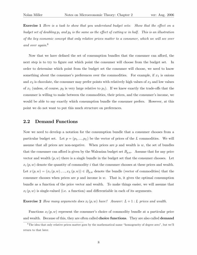
Exercise 1 Here is a task to show that you understand budget sets: Show that the effect on a
budget set of doubling p1 and p2 is the same as the effect of cutting w in half. This is an illustration
of the key economic concept that only relative prices matter to a consumer, which we will see over
and over again.6
Now that we have defined the set of consumption bundles that the consumer can afford, the
next step is to try to figure out which point the consumer will choose from the budget set. In
order to determine which point from the budget set the consumer will choose, we need to know
something about the consumer’s preferences over the commodities. For example, if x1 is onions
and x2 is chocolate, the consumer may prefer points with relatively high values of x2 and low values
of x1 (unless, of course, p2 is very large relative to p1). If we knew exactly the trade-offs that the
consumer is willing to make between the commodities, their prices, and the consumer’s income, we
would be able to say exactly which consumption bundle the consumer prefers. However, at this
point we do not want to put this much structure on preferences.
2.2 Demand Functions
Now we need to develop a notation for the consumption bundle that a consumer chooses from a
particular budget set. Let p = (p1, ..., pL) be the vector of prices of the L commodities. We will
assume that all prices are non-negative. When prices are p and wealth is w, the set of bundles
that the consumer can afford is given by the Walrasian budget set Bp,w. Assume that for any price
vector and wealth (p,w) there is a single bundle in the budget set that the consumer chooses. Let
xi (p,w) denote the quantity of commodity i that the consumer chooses at these prices and wealth.
Let x (p,w) = (x1 (p,w) , ..., xL (p,w)) ∈ Bp,w denote the bundle (vector of commodities) that the
consumer chooses when prices are p and income is w. That is, it gives the optimal consumption
bundle as a function of the price vector and wealth. To make things easier, we will assume that
xl (p,w) is single-valued (i.e. a function) and differentiable in each of its arguments.
Exercise 2 How many arguments does xl (p,w) have? Answer: L+ 1 : L prices and wealth.
Functions xl (p,w) represent the consumer’s choice of commodity bundle at a particular price
and wealth. Because of this, they are often called choice functions. They are also called demand6The idea that only relative prices matter goes by the mathematical name “homogeneity of degree zero”, but we’ll
return to that later.
8
Nolan Miller Notes on Microeconomic Theory: Chapter 2 ver: Aug. 2006
functions, although sometimes that name is reserved for choice functions that are derived from
the utility-maximization framework we’ll look at later. Generally, I use the terms interchangeably,
except when I want to emphasize that we are not talking about utility maximization, in which case
I’ll use the term “choice function.”
At this point, we should introduce an important distinction, the distinction between endoge-
nous and exogenous variables. An endogenous variable in an economic problem is a variable that
takes its value as a result of the behavior of one of the economic agents within the model. So, the
consumption bundle the consumer chooses x (p,w) is endogenous. An exogenous variable takes its
value from outside the model. Exogenous variables determine the constraints on the consumer’s
behavior. Thus in the consumer’s problem, the exogenous variables are prices and wealth. The
consumer cannot choose prices or wealth. But, prices and wealth determine the budget set, and
from the budget set the consumer chooses a consumption bundle. Hence the consumption bundle
is endogenous, and prices and wealth are exogenous. The consumer’s demand function x (p,w)
therefore gives the consumer’s choice as a function of the exogenous variables.
One of the main activities that economists do is try to figure out how endogenous variables
depend on exogenous variables, i.e., how consumers’ behavior depends on the constraints placed on
them (see principles 1-4 above).
2.3 Three Restrictions on Consumer Choices
So, let’s begin with the following question: What are the bare minimum requirements we can put
on behavior in order for them to be considered “reasonable,” and what can we say about consumers’
choices based on this? It turns out that relatively weak assumptions about consumer behavior can
generate strong requirements for how consumers should behave.7 We will start by enumerating
three requirements.
• Requirement 1: The consumer always spends her entire budget (Walras’ Law).
Requirement 1 is reasonable only if we are willing to make the assumption that “more is better.”
That is, for any commodity bundle x, the consumer would rather have a bundle with at least as
much of all commodities and strictly more of at least one commodity. Actually, we can get away
7A "weak assumption" imposes less restriction on the behavior of an economic agent than a "strong assumption"
does, so when designing a model, we prefer to use weaker assumptions if possible.
9

Nolan Miller Notes on Microeconomic Theory: Chapter 2 ver: Aug. 2006
with a weaker assumption: Given any bundle x, there is always a bundle that has more of at least
one commodity that the consumer strictly prefers to x. We’ll return to this later. For now, just
remember that the consumer spends all of her budget.
• Requirement 2: Only real opportunities matter (demand is homogeneous of degree zero).
The essence of requirement 2 is that consumers care about wealth and prices only inasmuch
as they affect the set of allocations in the budget set. Or, to put it another way, changes in the
environment that do not affect the budget set should not affect the consumer’s choices. So, for
example, if you double each price and wealth, the budget set is unchanged. Hence the consumer
can afford the same commodity bundles as before and should choose the same bundle as before.
• Requirement 3: Choices reveal information about (stable) preferences.
So, suppose I offer you a choice between an apple and a banana, and you choose an apple. Then
if tomorrow I see you eating a banana, I can infer that you weren’t offered an apple (remember
we assume that your preferences stay constant). Requirement 3 is known as the Weak Axiom of
Revealed Preference (WARP). The essence is this. Suppose that on occasion 1 you chose bundle
x when you could have chosen y. If I observe that on occasion 2 you choose bundle y, it must be
because bundle x was not available. Put slightly more mathematically, suppose two bundles x and
y are in the budget set Bp,w and the consumer chooses bundle x. Then if at some other prices and
wealth (p0, w0) the consumer chooses y, it must be that x was not in the budget set Bp0,w0 . We’ll
return to WARP later, but you can think of it in this way. If the consumer’s preferences remain
constant over time, then if x is preferred to y once, it should always be preferred to y. Thus if you
observe the consumer choose y, you can infer from this choice that x must not have been available.
Or, to put it another way, if you observe the consumer choosing x when x and y were available
on one day and y when x and y were available on the next day, then your model had better have
something in it to account for why this is so (i.e., a reason why the two days were different).
2.4 A First Analysis of Consumer Choices
In the rest of this chapter, we’ll develop formal notation for talking about consumer choices, show
how the three requirements on consumer behavior can be represented using this notation, and
determine what imposing these restrictions on consumer choices implies about the way consumers
10

Nolan Miller Notes on Microeconomic Theory: Chapter 2 ver: Aug. 2006
should behave when prices or wealth change. Thus it is our first pass at the four-step process of eco-
nomics: Assume consumers make choices that satisfy certain properties (the three requirements),
subject to some constraints (the budget set); assume further that any changes in choices are due
to changes in the constraints; and then derive testable predictions about consumer’s behavior.
2.4.1 Comparative Statics
The analytic method we will use to develop testable predictions is what economists call compar-
ative statics. A comparative statics analysis consists of coming up with a relationship between
the exogenous variables and the endogenous variables in a problem and then using calculus to
determine how the endogenous variables (i.e., the consumer’s choices) respond to changes in the
exogenous variables. Then, hopefully, we can tell if this response is positive, negative, or zero.8
We’ll see comparative statics analysis used over and over again. The important thing to remember
for now is that even though “comparative statics” as a phrase doesn’t mean anything, it refers to
figuring out how the endogenous variables depend on the exogenous variables.9
2.5 Requirement 1 Revisited: Walras’ Law
Requirement 1 for consumer choices is that consumers spend all of their wealth (Walras Law).
The implication of this is that given a budget set Bp,w, the consumer will choose a bundle on the
boundary of the budget set, sometimes called the budget frontier. The equation for the budget
frontier is the set of all commodity bundles that cost exactly w. Thus, Walras’ Law implies:
p · x (p,w) ≡ w.
When a consumer’s demand function x (p,w) satisfies this identity for all values of p and w, we
say that the consumer’s demand satisfies Walras’ Law. Thus the formal statement for “consumers
always spend all of their wealth” is that “demand functions satisfy Walras’ Law.”
8Although it would be nice to get a more precise measurement of the effects of changes in the exogenous parameters,
often we are only able to draw implications about the sign of the effect, unless we are willing to impose additional
restrictions on consumer demand.9The term “comparative statics” is meant to convey the idea that, while you analyze what happens before and
after the change in the exogenous parameter, you don’t analyze the process by which the change takes place.
11

Nolan Miller Notes on Microeconomic Theory: Chapter 2 ver: Aug. 2006
2.5.1 What’s the Funny Equals Sign All About?
Notice that in the expression of Walras’ Law, I wrote a funny, three-lined equals sign. Contrary
to popular belief, this doesn’t mean “really, really equal.” What it means is that, no matter what
values of p and w you choose, this relationship holds. For example, consider the equality:
2z = 1.
This is true for exactly one value of z, namely z = 12 . However, think about the following equality:
2z = a.
Suppose I were to ask you, for any value of a, tell me a value of z that makes this equality hold.
You could easily do this: z = a2 . Suppose I denote this by z (a) =
a2 . That is, z (a) is the value of z
that makes 2z = a true, given any value of a. If I substitute the function z (a) into the expression
2z = a, I get the following equation:
2z (a) = a.
Note that this expression is no longer a function of z. If I tell you a, you tell me z (a) (which is
a2 ), and no matter what value of a I choose, when I plug z (a) in on the left side of the equals, the
equality relation holds. Thus
2z (a) = a
holds for any value of a. We call an expression that is true for any value of the variable (in this
case a) an identity, and we write it with the fancy, three-lined equals sign in order to emphasize
this.
2z (a) ≡ a.
Why should we care if something is an equality or an identity? In a nut-shell, you can
differentiate both sides of an identity and the two sides remain equal. You can’t do this with
an equality. In fact, it doesn’t even make sense to differentiate both sides of an equality. To
illustrate this point, think again about the equality: 2x = 1. What happens if you increase x by
a small amount (i.e. differentiate with respect to x)? If you differentiate both sides with respect
to x, you get 2 = 0, which is not true.
On the other hand, think about 2z (a) ≡ a. We can ask the question what happens to z if you
increase a. We can answer this by differentiating both sides of the identity with respect to a. If
12
Nolan Miller Notes on Microeconomic Theory: Chapter 2 ver: Aug. 2006
you do this, you get
2dz (a)
da= 1
dz
da=
1
2
That is, if you increase a by 1, z increases by 12 . (If you don’t believe me, plug in some numbers
and confirm.)
It may seem to you like I’m making a big deal out of nothing, but this is really a critical
point. We are interested in determining how endogenous variables change in response to changes
in exogenous variables. In this case, z is our endogenous variable and a is our exogenous variable.
Thus, we are interested in things like dz(a)da . The only way we can determine these things is to get
identities that depend only on the exogenous variables and then differentiate them. Even if you
don’t quite believe me, you should keep this in mind. Eventually, it will become clear.
2.5.2 Back to Walras’ Law: Choice Response to a Change in Wealth
As we said, Walras’ Law is defined by the identity:
p · x (p,w) ≡ w
orLXl=1
plxl (p,w) ≡ w.
where the vector x(p,w) describes the bundle chosen:
x (p,w) = (x1 (p,w) , ..., xL (p,w))
Suppose we are interested in what happens to the bundle chosen if w increases a little bit. In other
words, how does the bundle the consumer chooses change if the consumer’s income increases by a
small amount? Since we have an identity defined in terms of the exogenous variables p and w, we
can differentiate both sides with respect to w:
d
dw
ÃLXl=1
plxl (p,w)
!≡ d
dww
Xl
pl∂xl (p,w)
∂w≡ 1. (2.1)
13

Nolan Miller Notes on Microeconomic Theory: Chapter 2 ver: Aug. 2006
So, now we have an expression relating the changes in the amount of commodities demanded in
response to a change in wealth. What does it say? The left hand side is the change in expenditure
due to the increase in wealth, and the right-hand side is the increase in wealth. Thus this expression
says that if wealth increases by 1 unit, total expenditure on commodities increases by 1 unit as
well. Thus the latter expression just restates Walras’ Law in terms of responses to changes in
wealth. Any change in wealth is accompanied by an equal change in expenditure. If you think
about it, this is really the only way that the consumer could satisfy Walras’ Law (i.e. spend all of
her money) both before and after the increase in wealth.
Based only on this expression,P
i pi∂xi(p,w)
∂w ≡ 1, what else can we say about the behavior of
the consumer’s choices in response to income changes? Well, first, think about ∂xi(p,w)∂w . Is this
expression going to be positive or negative? The answer depends on what kind of commodity
this is. Ordinarily, we think that if your wealth increases you will want to consume more of a
good. This is certainly true of goods like trips to the movies, meals at fancy restaurants, and
other “normal goods.” In fact, this is so much the normal case that we just go ahead and call such
goods - which have ∂xi(p,w)∂w > 0 - “normal goods.” But, you can also think about goods you want
to consume less of as your wealth goes up - cheap cuts of meat, cross-country bus trips, nights in
cheap motels, etc. All of these are things that, the richer you get, the less you want to consume
them. We call goods for which ∂xi(p,w)∂w < 0 “inferior goods.” Since x (p,w) depends on w, ∂xl(p,w)∂w
depends on w as well, which means that a good may be inferior at some levels of wealth but normal
at others.
So, what can we say based onP
i pi∂xi(p,w)
∂w ≡ 1? Well, this identity tells us that there is always
at least one normal good. Why? If all goods are inferior, then the terms on the left hand side are
all negative, and no matter how many negative terms you add together, they’ll never sum to 1.
2.5.3 Testable Implications
We can use this observation about normal goods to derive a testable implication of our theory.
Put simply, we have assumed that consumers spend all of the money they have on commodities.
Based on this, we conclude that following any change in wealth, total expenditure on goods should
increase by the same amount as wealth. If we knew prices and how much of the commodities
the consumer buys before and after the wealth change, we could directly test this. But, suppose
that we don’t observe prices. However, we believe that prices do not change when wealth changes.
What should we conclude if we observe that consumption of all commodities decreases following
14

Nolan Miller Notes on Microeconomic Theory: Chapter 2 ver: Aug. 2006
an increase in wealth? Unfortunately, the only thing we can conclude is that our theory is wrong.
People aren’t spending all of their wealth on commodities 1 through L.
Based on this observation, there are a number of possible directions to go. One possible
explanation is that there is another commodity, L+1, that we left out of our model, and if we had
accounted for that then we would see that consumption increased in response to the wealth increase
and everything would be right in the world. Another possible explanation is that in the world we
are considering, it is not the case that there is always something that the consumer would like more
of (which, you’ll recall, is the implicit assumption behind Walras’ Law). This would be the case,
for example, if the consumer could become satiated with the commodities, meaning that there is
a level of consumption beyond which you wouldn’t want to consume more even if you could. A
final possibility is that there is something wrong with the data and that if consumption had been
properly measured we would see that consumption of one of the commodities did, in fact, increase.
In any case, the next task of the intrepid economist is to determine which possible explanation
caused the failure of the theory and, if possible, develop a theory that agrees with the data.
2.5.4 Summary: How Did We Get Where We Are?
Let’s review the comparative statics methodology. First, we develop an identity that expresses a
relationship between the endogenous variables (consumption bundle) and the exogenous variable
of interest (wealth). The identity is true for all values of the exogenous variables, so we can
differentiate both sides with respect to the exogenous variables. Next, we totally differentiate the
identity with respect to a particular exogenous variable of interest (wealth). By rearranging, we
derive the effect of a change in wealth on the consumption bundle, and we try to say what we
can about it. In the previous example, we were able to make inferences about the sign of this
relationship. This is all there is to comparative statics.
2.5.5 Walras’ Law: Choice Response to a Change in Price
What are other examples of comparative statics analysis? Well, in the consumer model, the endoge-
nous variables are the amounts of the various commodities that the consumer chooses, xi(p,w).
We want to know how these things change as the restrictions placed on the consumer’s choices
change. The restriction put on the consumer’s choice by Walras’ Law takes the form of the budget
constraint, and the budget constraint is in turn defined by the exogenous variables — the prices
of the various commodities and wealth. We already looked at the comparative statics of wealth
15

Nolan Miller Notes on Microeconomic Theory: Chapter 2 ver: Aug. 2006
changes. How about the comparative statics of a price change?
Return to the Walras’ Law identity:
Xpixi (p,w) ≡ w.
Since this is an identity, we can differentiate with respect to the price of one of the commodities,
pj :
xj (p,w) +LXi=1
pi∂xi (p,w)
∂pj= 0. (2.2)
How does spending change in response to a price change? Well, if pj increases, spending on good
j increases, assuming that you continue to consume the same amount. This is captured by the
first term in (2.2). Of course, in response to the price change, you will also rearrange the products
you consume, purchasing more or less of the other products depending on whether they are gross
substitutes for good j or gross complements to good j.10 The effect of this rearrangement on total
expenditure is captured by the terms after the summation. Thus the meaning of (2.2) is that once
you take into account the increased spending in good j and the changes in spending associated
with rearranging the consumption bundle, total expenditure does not change. This is just another
way of saying that the consumer’s demand satisfies Walras’ Law.
2.5.6 Comparative Statics in Terms of Elasticities
The goal of comparative statics analysis is to determine the change in the endogenous variable
that results from a change in an exogenous variable. Sometimes it is more useful to think about
the percentage change in the endogenous variable that results from a percentage change in the
exogenous variable. Economists refer to the ratio of percentage changes as elasticities. Equations
(2.1) and (2.2), which are somewhat difficult to interpret in their current state, become much more
meaningful when written in terms of elasticities.
A price elasticity of demand gives the percentage change in quantity demanded associated with
a 1% change in price. Mathematically, price elasticity elasticity is defined as:
εipj =%∆xi%∆pj
=∂xi∂pj
· pjxi
Read εipj as “the elasticity of demand for good i with respect to the price of good j.”11
10The term ‘gross’ refers to the fact that wealth is held constant. It contrasts with the situation where utility is
held constant, where we drop the gross. All will become clear eventually.11Technically, the second equals sign in the equation above should be a limit, as %∆ −→ 0.
16
Nolan Miller Notes on Microeconomic Theory: Chapter 2 ver: Aug. 2006
Now recall equation (2.2):
xj (p,w) +LXi=1
pi∂xi (p,w)
∂pj= 0.
The terms that are summed look almost like elasticities, except that they need to be multiplied bypjxi. Perform the following sneaky trick. Multiply everything by pj
w , and multiply each term in the
summation by xixi(we can do this because xi
xi= 1 as long as xi 6= 0).
pjxj (p,w)
w+
LXi=1
pipjw
xixi
∂xi (p,w)
∂pj= 0
pjxj (p,w)
w+
LXi=1
pixiw
pjxi
∂xi (p,w)
∂pj= 0
bj (p,w) +LXi=1
bi (p,w) εipj = 0 (2.3)
where bj (p,w) is the share of total wealth the consumer spends on good j, known as the budget
share.
What does (2.3) mean? Consider raising the price of good j, pj , a little bit. If the consumer did
not change the bundle she consumes, this price change would increase the consumer’s total spending
by the proportion of her wealth she spends on good xj . This is known as a “wealth effect” since
it is as if the consumer has become poorer, assuming she does not change behavior. The wealth
effect is the first term, bj (p,w) . However, if good j becomes more expensive, the consumer will
choose to rearrange her consumption bundle. The effect of this rearrangement on total spending
will have to do with how much is spent on each of the goods, bi (p,w), and how responsive that
good is to changes in pj , as measured by εipj . Thus the terms after the sum represent the effect of
rearranging the consumption bundle on total consumption - these are known as substitution effects.
Hence the meaning of (2.3) is that when you combine the wealth effect and the substitution effects,
total expenditure cannot change. This, of course, is exactly what Walras’ Law says.
2.5.7 Why Bother?
In the previous section, we rearranged Walras’ Law by differentiating it and then manipulating the
resulting equation in order to get something that means exactly the same thing as Walras’ Law.
Why, then, did we bother? Hopefully, seeing Walras’ Law in other equations forms offers some
insight into what our model predicts for consumer behavior. Furthermore, many times it is easier
for economists to measure things like budget shares and elasticities than it is to measure actual
17
Nolan Miller Notes on Microeconomic Theory: Chapter 2 ver: Aug. 2006
quantities and prices. In particular, budget shares and elasticities do not depend on price levels,
but only on relative prices. Consequently it can be much easier to apply Walras’ Law when it is
written as (2.3) than when it is written as (2.2).
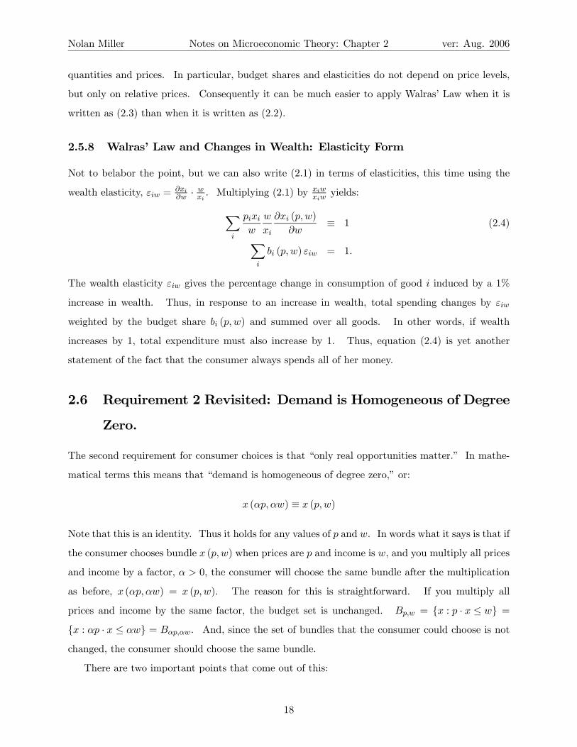
2.5.8 Walras’ Law and Changes in Wealth: Elasticity Form
Not to belabor the point, but we can also write (2.1) in terms of elasticities, this time using the
wealth elasticity, εiw = ∂xi∂w ·
wxi. Multiplying (2.1) by xiw
xiwyields:
Xi
pixiw
w
xi
∂xi (p,w)
∂w≡ 1 (2.4)X
i
bi (p,w) εiw = 1.
The wealth elasticity εiw gives the percentage change in consumption of good i induced by a 1%
increase in wealth. Thus, in response to an increase in wealth, total spending changes by εiw
weighted by the budget share bi (p,w) and summed over all goods. In other words, if wealth
increases by 1, total expenditure must also increase by 1. Thus, equation (2.4) is yet another
statement of the fact that the consumer always spends all of her money.
2.6 Requirement 2 Revisited: Demand is Homogeneous of Degree
Zero.
The second requirement for consumer choices is that “only real opportunities matter.” In mathe-
matical terms this means that “demand is homogeneous of degree zero,” or:
x (αp, αw) ≡ x (p,w)
Note that this is an identity. Thus it holds for any values of p and w. In words what it says is that if
the consumer chooses bundle x (p,w) when prices are p and income is w, and you multiply all prices
and income by a factor, α > 0, the consumer will choose the same bundle after the multiplication
as before, x (αp,αw) = x (p,w). The reason for this is straightforward. If you multiply all
prices and income by the same factor, the budget set is unchanged. Bp,w = {x : p · x ≤ w} =
{x : αp · x ≤ αw} = Bαp,αw. And, since the set of bundles that the consumer could choose is not
changed, the consumer should choose the same bundle.
There are two important points that come out of this:
18

Nolan Miller Notes on Microeconomic Theory: Chapter 2 ver: Aug. 2006
1. This is an expression of the belief that changes in behavior should come from changes in
the set of available alternatives. Since the rescaling of prices and income do not affect the budget
set, they should not affect the consumer’s choice.
2. The second point is that nominal prices are meaningless in consumer theory. If you tell
me that a loaf of bread costs $10, I need to know what other goods cost before I can interpret the
first statement. And, in terms of analysis, this means that we can always “normalize” prices by
arbitrarily setting one of them to whatever we like (often it is easiest to set it equal to 1), since
only the real prices matter and fixing one commodity’s nominal price will not affect the relative
values of the other prices.
Exercise 3 If you don’t believe me that this change doesn’t affect the budget set, you should go
back to the two-commodity example, plug in the numbers and check it for yourself. If you can’t do
it with the general scaling factor α, you should let α = 2 and try it for that. Most of the time,
things that are hard to understand with general parameter values like α, p,w are simple once you
plug in actual numbers for them and churn through the algebra.
2.6.1 Comparative Statics of Homogeneity of Degree Zero
We can also perform a comparative statics analysis of the requirement that demand be homogeneous
of degree zero, i.e. only real opportunities matter. What does this imply for choice behavior?
The homogeneity assumption applies to proportional changes in all prices and wealth:
xi (αp, αw) ≡ xi (p,w) for all i, α > 0.
To make things clear, let the initial price vector be denoted p0 =¡p01, ..., p
0L
¢and let w0 original
wealth, and (for the time being) assume that L = 2. For example,¡p0, w0
¢could be p0 = (3, 2)
and w0 = 7. Before we differentiate, I want to make sure that we’re clear on what is going on.
So, rewrite the above expression as:
xi¡αp01, αp
02, αw
0¢≡ xi
¡p01, p
02, w
0¢. (2.5)
Now, notice that on the left-hand side for any α > 0 the price of good 1 is p1 = αp01, the price of
good 2 is p2 = αp02, and wealth is w = αw0. That is, given α. We are interested in what happens
to demand as α changes, so it is important to recognize that the prices and wealth are functions of
α.
19

Nolan Miller Notes on Microeconomic Theory: Chapter 2 ver: Aug. 2006
We are interested in what happens to demand when, beginning at original prices p0 and wealth
w0, we scale up all prices and wealth proportionately. To do this, we want to see what happens
when we increase α, starting at α = 1. Because the prices and wealth are functions of α, we have
to use the Chain Rule in evaluating the derivative of (2.5) with respect to α. Differentiating (2.5)
with respect to α yields:
∂xi¡αp01, αp
02, αw
0¢
∂p1
∂p1∂α
+∂xi
¡αp01, αp
02, αw
0¢
∂p2
∂p2∂α
+∂xi
¡αp01, αp
02, αw
0¢
∂w
∂w
∂α≡ 0.
Since p1 = αp01,∂p1∂α = p01, and similarly
∂p2∂α = p02, and
∂w∂a = w0, so this expression becomes:
∂xi¡αp01, αp
02, αw
0¢
∂p1p01 +
∂xi¡αp01, αp
02, αw
0¢
∂p2p02 +
∂xi¡αp01, αp
02, αw
0¢
∂ww0 ≡ 0. (2.6)
Notice that the first line takes the standard Chain Rule form: for each argument (p1, p2, and w),
take the partial derivative of the function with respect to that argument and multiply it by the
derivative with respect to α of “what’s inside” the argument.12
Finally, notice that (2.6) has prices and wealth¡αp01, αp
02, αw
0¢. We are asking the question
“what happens to xi when prices and wealth begin at¡p01, p
02, w
0¢and are all increased slightly
by the same proportion?” In order to make sure we are answering this question, we need to set
α = 1, so that the partial derivatives are evaluated at the original prices and wealth. Evaluating
the last expression at α = 1 yields the following expression in terms of the original price-wealth
vector (s1, s2, v) :
∂xi¡p01, p
02, w
0¢
∂p1p01 +
∂xi¡p01, p
02, w
0¢
∂p2p02 +
∂xi¡p01, p
02, w
0¢
∂ww0 ≡ 0. (2.7)
Generalizing the previous argument to the case where L is any positive number, expression (2.7)
becomes:∂xi
¡p0, w0
¢∂w
w0 +LXj=1
∂xi¡p0, w0
¢∂pj
p0j = 0 for all i. (2.8)
This is where we need to face an ugly fact. Economists are terrible about notation, which
makes this stuff harder to learn than it needs to be. When you see (2.8) written in a textbook, it
will look like this:∂xi (p,w)
∂ww +
LXj=1
∂xi (p,w)
∂pjpj = 0 for all i.
12 If you are confused, see the next subsection for further explanation.
20

Nolan Miller Notes on Microeconomic Theory: Chapter 2 ver: Aug. 2006
That is, they drop the superscript “0” that denotes the original price vector. But, notice that the
symbol “w” in this expression has two different meanings. The “w” in “∂w” in the denominator
of the first term says “we’re differentiating with respect to the wealth argument,” while the “w”
in “∂xi (p,w)” and the “w” multiplying this term refer to the original wealth level, i.e., the wealth
level at which the expression is being evaluated. Similarly, “pj” also has two different meanings in
this expression. To make things worse, economists frequently skip steps in derivations.13
It is straightforward to get an elasticity version of (2.8). Just divide through by xi (p,w):
εiw +LXj=1
εipj = 0. (2.9)
Elasticities εiw and εipj give the elasticity of the consumer’s demand response to changes in wealth
and the price of good j, respectively. The total percentage change in consumption of good i is
given by summing the percentage changes due to changes in wealth and in each of the prices.
Homogeneity of degree zero says that in response to proportional changes in all prices and wealth
the total change in demand for each commodity should not change. This is exactly what (2.9)
says.
2.6.2 A Mathematical Aside ...
If this is unfamiliar to you, the computation may seem strange. If it doesn’t seem strange, then
skip on to the next section.
If you’re still here, let’s try it one more time. This time, we’ll let L = 2, and choose specific
values for the prices and wealth. Let good 1’s price be 5, good 2’s price be 3, and wealth be 10
initially. Then, (2.5) writes as:
xi (5α, 3α, 10α) ≡ xi (5, 3, 10) .
Now, starting at prices (5, 3) and wealth 10, we are interested in what happens to demand for xi
as we increase all prices and wealth proportionately. To do this, we will first increase α by a
small amount (i.e., differentiate with respect to α), and then we’ll evaluate the resulting expression
at α = 1. This will give us an expression for the effect of a small increase in α. So, totally
differentiate both sides with respect to α :
∂xi (5α, 3α, 10α)
∂p1
d (5α)
dα+
∂xi (5α, 3α, 10α)
∂p2
d (3α)
dα+
∂xi (5α, 3α, 10α)
∂w
d (10α)
dα≡ 0
∂xi (5α, 3α, 10α)
∂p15 +
∂xi (5α, 3α, 10α)
∂p23 +
∂xi (5α, 3α, 10α)
∂w10 ≡ 0.
13These are a couple of the main reasons why documents such as these are needed.
21

Nolan Miller Notes on Microeconomic Theory: Chapter 2 ver: Aug. 2006
Again, the partial derivatives ∂xi∂pj
denote the partial derivative of function xi (p,w) with respect to
the “pj slot,” i.e., the jth argument of the function. And, since we are interested in what happens
when you increase all prices and wealth proportionately beginning from prices (5, 3) and wealth 10,
we would like the left-hand side to be evaluated at (5, 3, 10). To get this, set α = 1 :
∂xi (5, 3, 10)
∂p15 +
∂xi (5, 3, 10)
∂p23 +
∂xi (5, 3, 10)
∂w10 ≡ 0 (2.10)
Comparing this expression with (2.7) shows that the role of p∗1, p∗2, and w∗ are played by 5, 3, and
10, respectively in (2.10), as is expected.
The source of confusion in understanding this derivation seems to lie in confusing the partial
derivative of xi with respect to the p1 argument (for example) with the particular price of good
1, which is 5α in this example and αp∗1 in the more general derivation above. The key is to notice
that, in applying the chain rule, you always differentiate the function (e.g., xi ()) with respect to
its argument (e.g., p1), and then differentiate the function that is in the argument’s “slot” (e.g., 5α
or αs1 or αp1 if you are an economist) with respect to α.
2.7 Requirement 3 Revisited: The Weak Axiom of Revealed Pref-
erence
The third requirement that we will place on consumer choices is that they satisfy the Weak Axiom
of Revealed Preference (WARP). To remind you of the informal definition, WARP is a requirement
of consistency in decision-making. It says that if a consumer chooses z when y was also affordable,
this choice reveals that the consumer prefers z to y. Since we assume that consumer preferences are
constant and we have modeled all of the relevant constraints on consumer behavior and preferences,
if we ever observe the consumer choose y, it must be that z was not available (since if it were, the
consumer would have chosen z over y since she had previously revealed her preference for z). We
now turn to the formal definition.
Definition 4 Consider any two distinct price-wealth vectors (p,w) and (p0, w0) 6= (p,w). Let
z = x (p,w) and y = x (p0, w0). The consumer’s demand function satisfies WARP if whenever
p · y ≤ w, p0 · z > w0.
We can restate the last part of the definition as: if y ∈ Bp,w, then z /∈ Bp0,w0 . If y could have
been chosen when z was chosen, then the consumer has revealed that she prefers z to y. Therefore
22

Nolan Miller Notes on Microeconomic Theory: Chapter 2 ver: Aug. 2006
if you observe her choose y, it must be that z was not available. I apologize for repeating the same
definition over and over, but a) it helps to attach words to the math, and b) if you wanted math
without explanation you could read a textbook.
In its basic form, WARP does not generate any predictions that can immediately be taken to
the data and tested. But, if we rearrange the statement a little bit, we can get an easily testable
prediction. So, let me ask the WARP question a different way. Suppose the consumer chooses z
when prices and wealth are (p,w) , and z is affordable when prices and wealth are (p0, w0). What
does WARP tell us about which bundles the consumer could choose when prices are (p0, w0)?
There are two choices to consider: either x (p0, w0) = z. This is perfectly admissible under
WARP. The other choice is that x (p0, w0) = y 6= z. In this case, WARP will place restrictions on
which bundles y can be chosen. What are they? By virtue of the fact that z was chosen when
prices and wealth were (p,w), we know that y /∈ Bp,w, since if it were there would be a violation
of WARP. Thus it must be that if the consumer chooses a bundle y different than x at (p0, w0), y
must not have been affordable when prices and wealth were (p,w).
This is illustrated graphically in figure 2.F.1 in MWG (p. 30). In panel a, since x (p0, w0) is
chosen at (p0, w0), when prices are (p00, w00) the consumer must either choose x (p0, w0) again or a
bundle x (p00, w00) that is not in Bp0,w0 . If we assume that demand satisfies Walras’ Law as well,
x (p00, w00) must lay on the frontier. Thus if x (p0, w0) is as drawn, it cannot be chosen at prices
(p00, w00). The chosen bundle must lay on the segment of Bp00,w00 below and to the right of the
intersection of the two budget lines, as does x (p00, w00). Similar reasoning holds in panel b. The
chosen bundle cannot lay within Bp0,w0 if WARP holds. Panel c depicts the case where x (p0, w0) is
affordable both before and after the change in prices and wealth. In this case, x (p0, w0) could have
been chosen after the price change. But, if it is not chosen at (p00, w00), then the chosen bundle
must lay outside of Bp00,w00 , as does x (p00, w00) . In panels d and e, x (p00, w00) ∈ Bp0,w0 , and thus this
behavior does not satisfy WARP.
2.7.1 Compensated Changes and the Slutsky Equation
Panel c in MWG Figure 2.F.1 suggests a way in which WARP can be used to generate predictions
about behavior. Imagine two different price-wealth vectors, (p,w) and (p0, w0), such that bundle
z = x (p,w) lies on the frontier of both Bp,w and Bp0,w0 . This corresponds to the following
hypothetical situation. Suppose that originally prices are (p,w) and you choose bundle z = x (p,w).
I tell you that I am going to change the price vector to p0. But, I am fair, and so I tell you that in
23
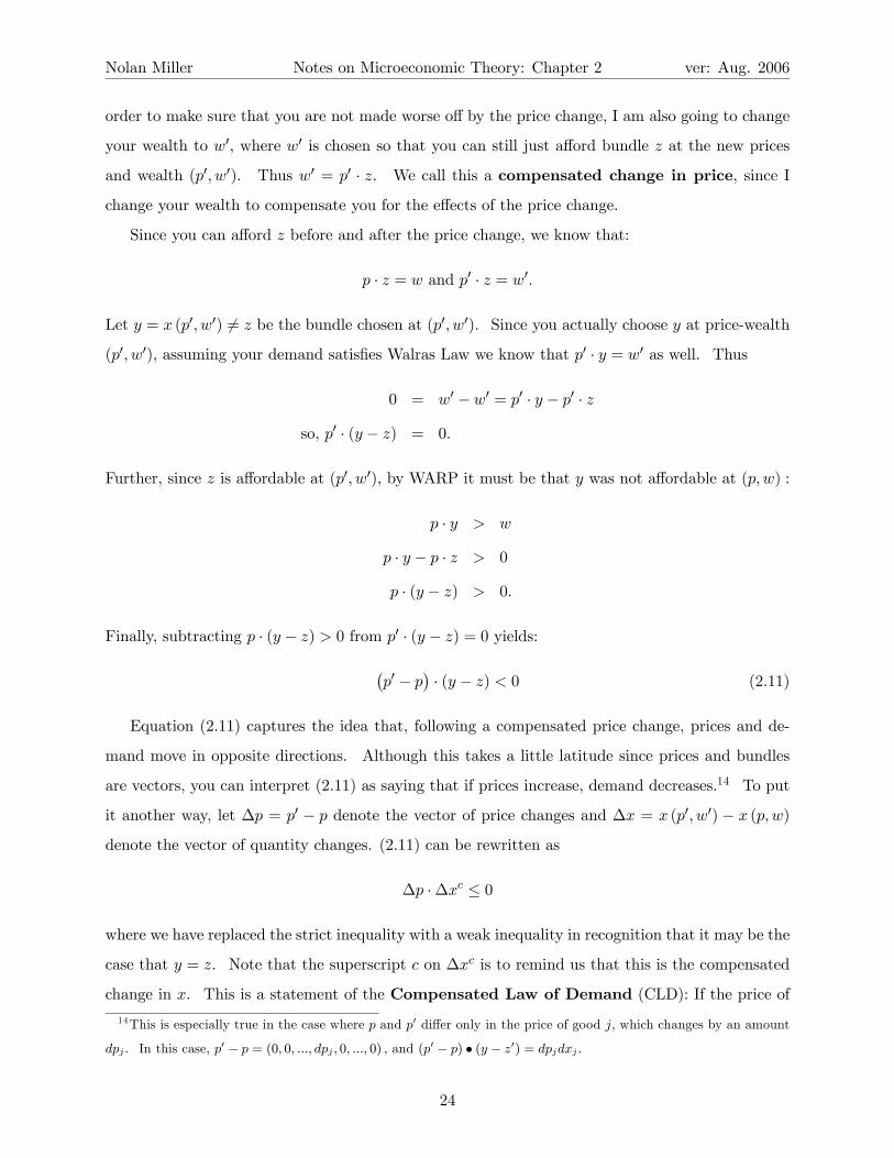
Nolan Miller Notes on Microeconomic Theory: Chapter 2 ver: Aug. 2006
order to make sure that you are not made worse off by the price change, I am also going to change
your wealth to w0, where w0 is chosen so that you can still just afford bundle z at the new prices
and wealth (p0, w0). Thus w0 = p0 · z. We call this a compensated change in price, since I
change your wealth to compensate you for the effects of the price change.
Since you can afford z before and after the price change, we know that:
p · z = w and p0 · z = w0.
Let y = x (p0, w0) 6= z be the bundle chosen at (p0, w0). Since you actually choose y at price-wealth
(p0, w0), assuming your demand satisfies Walras Law we know that p0 · y = w0 as well. Thus
0 = w0 − w0 = p0 · y − p0 · z
so, p0 · (y − z) = 0.
Further, since z is affordable at (p0, w0), by WARP it must be that y was not affordable at (p,w) :
p · y > w
p · y − p · z > 0
p · (y − z) > 0.
Finally, subtracting p · (y − z) > 0 from p0 · (y − z) = 0 yields:
¡p0 − p
¢· (y − z) < 0 (2.11)
Equation (2.11) captures the idea that, following a compensated price change, prices and de-
mand move in opposite directions. Although this takes a little latitude since prices and bundles
are vectors, you can interpret (2.11) as saying that if prices increase, demand decreases.14 To put
it another way, let ∆p = p0 − p denote the vector of price changes and ∆x = x (p0, w0) − x (p,w)
denote the vector of quantity changes. (2.11) can be rewritten as
∆p ·∆xc ≤ 0
where we have replaced the strict inequality with a weak inequality in recognition that it may be the
case that y = z. Note that the superscript c on ∆xc is to remind us that this is the compensated
change in x. This is a statement of the Compensated Law of Demand (CLD): If the price of14This is especially true in the case where p and p0 differ only in the price of good j, which changes by an amount
dpj . In this case, p0 − p = (0, 0, ..., dpj , 0, ..., 0) , and (p0 − p) • (y − z0) = dpjdxj .
24
Nolan Miller Notes on Microeconomic Theory: Chapter 2 ver: Aug. 2006
a commodity goes up, you demand less of it. If we take a calculus view of things, we can rewrite
this in terms of differentials: dp · dxc ≤ 0.
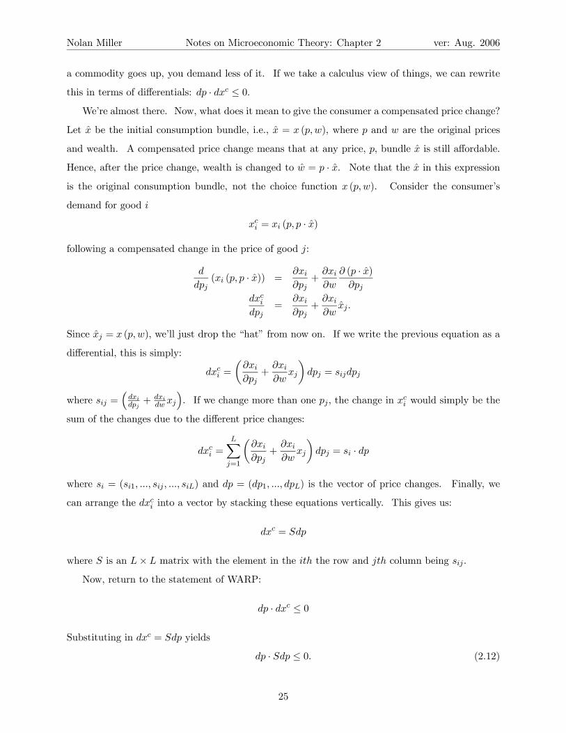
We’re almost there. Now, what does it mean to give the consumer a compensated price change?
Let x be the initial consumption bundle, i.e., x = x (p,w), where p and w are the original prices
and wealth. A compensated price change means that at any price, p, bundle x is still affordable.
Hence, after the price change, wealth is changed to w = p · x. Note that the x in this expression
is the original consumption bundle, not the choice function x (p,w). Consider the consumer’s
demand for good i
xci = xi (p, p · x)
following a compensated change in the price of good j:
d
dpj(xi (p, p · x)) =
∂xi∂pj
+∂xi∂w
∂ (p · x)∂pj
dxcidpj
=∂xi∂pj
+∂xi∂w
xj .
Since xj = x (p,w), we’ll just drop the “hat” from now on. If we write the previous equation as a
differential, this is simply:
dxci =
µ∂xi∂pj
+∂xi∂w
xj
¶dpj = sijdpj
where sij =³dxidpj+ dxi
dw xj
´. If we change more than one pj , the change in xci would simply be the
sum of the changes due to the different price changes:
dxci =LXj=1
µ∂xi∂pj
+∂xi∂w
xj
¶dpj = si · dp
where si = (si1, ..., sij , ..., siL) and dp = (dp1, ..., dpL) is the vector of price changes. Finally, we
can arrange the dxci into a vector by stacking these equations vertically. This gives us:
dxc = Sdp
where S is an L× L matrix with the element in the ith the row and jth column being sij .
Now, return to the statement of WARP:
dp · dxc ≤ 0
Substituting in dxc = Sdp yields
dp · Sdp ≤ 0. (2.12)
25

Nolan Miller Notes on Microeconomic Theory: Chapter 2 ver: Aug. 2006
Inequality (2.12) has a mathematical significance: It implies that matrix S, which we will call the
substitution matrix, is negative semi-definite. What this means is that if you pre- and post-multiply
S by the same vector, the result is always a non-positive number. This is important because
mathematicians have figured out a bunch of nice properties of negative semi-definite matrices.
Among them are:
1. The principal-minor determinants of S follow a known pattern.
2. The diagonal elements sii are non-positive. (Generally, they will be strictly negative, but we
can’t show that based on what we’ve done so far).
3. Note that WARP does not imply that S is symmetric. This is the chief difference between
the choice-based approach and the preference-based approach we will consider later.
All I want to say about #1 is this. Basically, it amounts to knowing that the second-order
conditions for a certain maximization problem are satisfied. But, in this course we aren’t going
to worry about second-order conditions. So, file it away that if you ever need to know anything
about the principal minors of S, you can look it up in a book.
Item #2 is a fundamental result in economics, because it says that the change in demand for
a good in response to a compensated price increase is negative. In other words, if price goes up,
demand goes down. This is the Compensated Law of Demand (CLD). You may be thinking
that it was a lot of work to derive something so obvious, but the fact that the CLD is derived from
WARP and Walras’ Law is actually quite important. If these were not sufficient for the CLD,
which we know from observation to be true, then that would be a strong indicator that we have
left something out of our model.
The fact that sii ≤ 0 can be used to help explain an anomaly of economic theory, the Giffen
good. Ordinarily, we think that if the price of a good increases, holding wealth constant, the
demand for that good will decrease. This is probably what you thought of as the “Law of Demand,”
even though it isn’t always true. Theoretically, it is possible that when the price of a good increases,
a consumer actually chooses to consume more of it. By way of motivation, think of the following
story. A consumer spends all of her money on two things: food and trips to Hawaii. Suppose
the price of food increases. It may be that after the increase, the consumer can no longer afford
the trip to Hawaii and therefore spends all of her money on food. The result is that the consumer
actually buys more food than she did before the price increase.
26

Nolan Miller Notes on Microeconomic Theory: Chapter 2 ver: Aug. 2006
How does this story manifest itself in the theory we have learned up until now? We know that:
sii =
µ∂xi∂pi
+∂xi∂w
xi
¶Rearranging it:
∂xi (p,w)
∂pi= sii −
∂xi∂w
xi.
We know that sii ≤ 0 since S is negative semi-definite. Clearly, xi ≥ 0. But, what happens if xiis a strongly inferior good? In this case, ∂xi
∂w < 0, meaning −∂xi∂w xi > 0. And, if the magnitude of
−∂xi∂w xi is greater than sii, it can be that ∂xi
∂pi> 0, which is what it means to be a Giffen good.
What does the theory tell us? Well, it tells us that in order for a good to be a Giffen good, it
must be a strongly inferior good. Or, to put it the other way, a normal good cannot be a Giffen
good.15
Before going on, let me give one more aside on why we bother with all of this stuff. Remember
when I started talking about increasing prices, and I said that I was fair, so I was going to also
change your wealth? Well, it turns out that a good measure of the impact of a price change on
a consumer is given by the change in wealth it would take to compensate you for a price change.
So, if we could observe the sii terms, this would help us to measure the impact of price changes on
consumers. But, the problem is that we never observe compensated price changes, we only observe
the uncompensated ones, dxi(p,w)dpi
. But, the relationship above gives us a way to recover sii from
observations on uncompensated price changes ∂xi∂pi, wealth changes, ∂xi
∂w , and actual consumption,
xi. Thus the importance of the relationship sii =³∂xi∂pi+ ∂xi
∂w xi
´is that it allows us to recover an
unobservable quantity that we are interested it, sii, from observables.
2.7.2 Other Properties of the Substitution Matrix
Based on what we know about demand functions, we can also determine a couple of additional
properties of the Substitution matrix. They are:
p · S (p,w) = 0
S (p,w) p = 0
15Technically, it is not the goods that are Giffen. Rather, the consumer’s behavior at a particular price-wealth
combination is Giffen. For example, it has been shown that very poor consumers in China exhibit Giffen behavior:
their demand curve for rice slopes upward in the price of rice. But, non-poor consumers do not exhibit Giffen
behavior: their demand curve slopes downward. See R. Jensen and N. Miller (2001).
27

Nolan Miller Notes on Microeconomic Theory: Chapter 2 ver: Aug. 2006
These can be derived from the comparative statics implications of Walras’ Law and homogeneity
of degree zero. Their effect is to impose additional restrictions on the set of admissible demand
functions. So, suppose you get some estimates of ∂xi∂pj, p, w, and ∂xi
∂w , which can all be computed
from data, and you are concerned with whether you have a good model. One thing you can do
is compute S from the data, and check to see if the two equations above hold. If they do, you’re
doing okay. If they don’t, this is a sign that your data do not match up with your theory. This
could be due to data problems or to theory problems, but in either case it means that you have
work to do.16
16The usual statistical procedure in this instance is to impose these conditions as restrictions on the econometric
model and then test to see if they are valid. I leave it to people who know more econometrics than I do to explain
how.
28

Chapter 3
The Traditional Approach to
Consumer Theory
In the previous section, we considered consumer behavior from a choice-based point of view. That
is, we assumed that consumers made choices about which consumption bundle to choose from a set
of feasible alternatives, and, using some rather mild restrictions on choices (homogeneity of degree
zero, Walras’ law, and WARP), were able make predictions about consumer behavior. Notice that
our predictions were entirely based on consumer behavior. In particular, we never said anything
about why consumers behave the way they do. We only hold that the way they behave should be
consistent in certain ways.
The traditional approach to consumer behavior is to assume that the consumer has well-defined
preferences over all of the alternative bundles and that the consumer attempts to select the most
preferred bundle from among those bundles that are available. The nice thing about this approach is
that it allows us to build into our model of consumer behavior how the consumer feels about trading
off one commodity against another. Because of this, we are able to make more precise predictions
about behavior. However, at some point people started to wonder whether the predictions derived
from the preference-based model were in keeping with the idea that consumers make consistent
choices, or whether there could be consistent choice-based behavior that was not derived from the
maximization of well-defined preferences. It turns out that if we define consistent choice making
as homogeneity of degree zero, Walras’ law, and WARP, then there are consistent choices that
cannot be derived from the preference-based model. But, if we replace WARP with a slightly
stronger but still reasonable condition, called the Strong Axiom of Revealed Preference (SARP),
29
Nolan Miller Notes on Microeconomic Theory: Chapter 3 ver: Aug. 2006
then any behavior consistent with these principles can be derived from the maximization of rational
preferences.
Next, we take up the traditional approach to consumer theory, often called “neoclassical” con-
sumer theory.
3.1 Basics of Preference Relations
We’ll continue to assume that the consumer chooses from among L commodities and that the
commodity space is given by X ⊂ RL+. The basic idea of the preference approach is that given any
two bundles, we can say whether the first is “at least as good as” the second. The “at-least-as-
good-as” relation is denoted by the curvy greater-than-or-equal-to sign: º. So, if we write x º y,
that means that “x is at least as good as y.”
Using º, we can also derive some other preference relations. For example, if x º y, we
could also write y ¹ x, where ¹ is the “no better than” relation. If x º y and y º x, we say
that a consumer is “indifferent between x and y,” or symbolically, that x ∼ y. The indifference
relation is important in economics, since frequently we will be concerned with indifference sets.
The indifference curve Iy is defined as the set of all bundles that are indifferent to y. That is,
Iy = {x ∈ X|y ∼ x}. Indifference sets will be very important as we move forward, and we will
spend a great deal of time and effort trying to figure out what they look like, since the indifference
sets capture the trade-offs the consumer is willing to make among the various commodities. The
final preference relation we will use is the “strictly better than” relation. If x is at least as good
as y and y is not at least as good as x, i.e., x º y and not y º x (which we could write y ² x), we
say that x  y, or x is strictly better than (or strictly preferred to) y.
Our preference relations are all examples of mathematical objects called binary relations. A
binary relation compares two objects, in this case, two bundles. For instance, another binary
relation is “less-than-or-equal-to,” ≤. There are all sorts of properties that binary relations can
have. The first two we will be interested in are called completeness and transitivity. A binary
relation is complete if, for any two elements x and y in X, either x º y or y º x. That is, any two
elements can be compared. A binary relation is transitive if x º y and y º z imply x º z. That
is, if x is at least as good as y, and y is at least as good as z, then x must be at least as good as z.
The requirements of completeness and transitivity seem like basic properties that we would like
any person’s preferences to obey. This is true. In fact, they are so basic that they form economists’
30

Nolan Miller Notes on Microeconomic Theory: Chapter 3 ver: Aug. 2006
very definition of what it means to be rational. That is, a preference relation º is called rational
if it is complete and transitive.
When we talked about the choice-based approach, we said that there was implicit in the idea
that demand functions satisfy Walras Law the idea that “more is better.” This idea is formalized
in terms of preferences by making assumptions about preferences over one bundle or another.
Consider the following property, called monotonicity:
Definition 5 A preference relation º is monotone if x  y for any x and y such that xl > yl
for l = 1, ..., L. It is strongly monotone if xl ≥ yl for all l = 1, ..., L and xj > yj for some
j ∈ {1, ..., L} implies that x  y.
Monotonicity and strong monotonicity capture two different notions of “more is better.” Monotonic-
ity says that if every component of x is larger than the corresponding component of y, then x is
strictly preferred to y. Strong monotonicity is the requirement that if every component of x is at
least as large (but not necessarily strictly larger) than the corresponding component of y and at
least one component of x is strictly larger, x is strictly preferred to y.
The difference between monotonicity and strong monotonicity is illustrated by the following
example. Consider the bundles x = (1, 1) and y = (1, 2). If º is strongly monotone, then we
can say that y  x. However, if º is monotone but not strongly monotone, then it need not be
the case that y is strictly preferred to x. Since preference relations that are strongly monotone
are monotone, but preferences that are monotone are not necessarily strongly monotone, strong
monotonicity is a more restrictive (a.k.a. “stronger”) assumption on preferences.
If preferences are monotone or strongly monotone, it follows immediately that a consumer will
choose a bundle on the boundary of the Walrasian budget set. Hence an assumption of some sort
of monotonicity must have been in the background when we assumed consumer choices obeyed
Walras’ Law. However, choice behavior would satisfy Walras’ Law even if preferences satisfied the
following weaker condition, called local nonsatiation.
Condition 6 A preference relation º satisfies local nonsatiation if for every x and every ε > 0
there is a point y such that ||x− y|| ≤ ε and y  x.
That is, for every x, there is always a point “nearby” that the consumer strictly prefers to x,
and this is true no matter how small you make the definition of “nearby.” Local nonsatiation allows
for the fact that some commodities may be “bads” in the sense that the consumer would sometimes
31
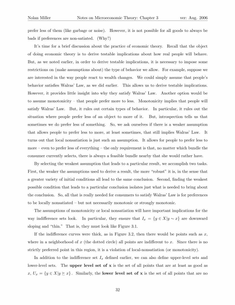
Nolan Miller Notes on Microeconomic Theory: Chapter 3 ver: Aug. 2006
prefer less of them (like garbage or noise). However, it is not possible for all goods to always be
bads if preferences are non-satiated. (Why?)
It’s time for a brief discussion about the practice of economic theory. Recall that the object
of doing economic theory is to derive testable implications about how real people will behave.
But, as we noted earlier, in order to derive testable implications, it is necessary to impose some
restrictions on (make assumptions about) the type of behavior we allow. For example, suppose we
are interested in the way people react to wealth changes. We could simply assume that people’s
behavior satisfies Walras’ Law, as we did earlier. This allows us to derive testable implications.
However, it provides little insight into why they satisfy Walras’ Law. Another option would be
to assume monotonicity — that people prefer more to less. Monotonicity implies that people will
satisfy Walras’ Law. But, it rules out certain types of behavior. In particular, it rules out the
situation where people prefer less of an object to more of it. But, introspection tells us that
sometimes we do prefer less of something. So, we ask ourselves if there is a weaker assumption
that allows people to prefer less to more, at least sometimes, that still implies Walras’ Law. It
turns out that local nonsatiation is just such an assumption. It allows for people to prefer less to
more — even to prefer less of everything — the only requirement is that, no matter which bundle the
consumer currently selects, there is always a feasible bundle nearby that she would rather have.
By selecting the weakest assumption that leads to a particular result, we accomplish two tasks.
First, the weaker the assumptions used to derive a result, the more “robust” it is, in the sense that
a greater variety of initial conditions all lead to the same conclusion. Second, finding the weakest
possible condition that leads to a particular conclusion isolates just what is needed to bring about
the conclusion. So, all that is really needed for consumers to satisfy Walras’ Law is for preferences
to be locally nonsatiated — but not necessarily monotonic or strongly monotonic.
The assumptions of monotonicity or local nonsatiation will have important implications for the
way indifference sets look. In particular, they ensure that Ix = {y ∈ X|y ∼ x} are downward
sloping and “thin.” That is, they must look like Figure 3.1.
If the indifference curves were thick, as in Figure 3.2, then there would be points such as x,
where in a neighborhood of x (the dotted circle) all points are indifferent to x. Since there is no
strictly preferred point in this region, it is a violation of local-nonsatiation (or monotonicity).
In addition to the indifference set Ix defined earlier, we can also define upper-level sets and
lower-level sets. The upper level set of x is the set of all points that are at least as good as
x, Ux = {y ∈ X|y º x} . Similarly, the lower level set of x is the set of all points that are no
32

Nolan Miller Notes on Microeconomic Theory: Chapter 3 ver: Aug. 2006
x2
x1
Ix
Figure 3.1: Thin Indifferent Sets
x2
x1
Ix
x
Figure 3.2: Thick Indifference Sets
33

Nolan Miller Notes on Microeconomic Theory: Chapter 3 ver: Aug. 2006
better than x, Lx = {y ∈ X|x º y}. Just as monotonicity told us something about the shape of
indifference sets, we can also make assumptions that tell us about the shape of upper and lower
level sets.
Recall that a set of points, X, is convex if for any two points in the set the (straight) line
segment between them is also in the set.1 Formally, a set X is convex if for any points x and x0
in X, every point z on the line joining them, z = tx + (1− t)x0 for some t ∈ [0, 1], is also in X.
Basically, a convex set is a set of points with no holes in it and with no “notches” in the boundary.
You should draw some pictures to figure out what I mean by no holes and no notches in the set.
Before we move on, let’s do a thought experiment. Consider two possible commodity bundles,
x and x0. Relative to the extreme bundles x and x0, how do you think a typical consumer feels
about an average bundle, z = tx + (1− t)x0, t ∈ (0, 1)? Although not always true, in general,
people tend to prefer bundles with medium amounts of many goods to bundles with a lot of some
things and very little of others. Since real people tend to behave this way, and we are interested in
modeling how real people behave, we often want to impose this idea on our model of preferences.2
Exercise 7 Confirm the following two statements: 1) If º is convex, then if y º x and z º x,
ty + (1− t) z º x as well. (2) Suppose x ∼ y. If º is convex, then for any z = ty + (1− t)x,
z º x.
Another way to interpret convexity of preferences is in terms of a diminishing marginal rate
of substitution (MRS), which is simply the slope of the indifference curve. The idea here is that
if you are currently consuming a bundle x, and I offer to take some x1 away from you and replace
it with some x2, I will have to give you a certain amount of x2 to make you exactly indifferent for
the loss of x1. A diminishing MRS means that this amount of x2 I have to give you increases the
more x2 that you already are consuming - additional units of x2 aren’t as valuable to you.
The upshot of the convexity and local non-satiation assumptions is that indifference sets have to
be thin, downward sloping, and be “bowed upward.” There is nothing in the definition of convexity1This is the definition of a convex set. It should not be confused with a convex function, which is a different
thing altogether. In addition, there is such thing as a concave function. But, there is no such thing as a
concave set. I sympathize with the fact that this terminology can be confusing. But, that’s just the way it is.
My advice is to focus on the meaning of the concepts, i.e., “a set with no notches and no holes.”2 It is only partly true that when we assume preferences are convex we do so in order to capture real behavior. In
addition, the basic mathematical techniques we use to solve our problems often depend on preferences being convex.
If they are not (and one can readily think of examples where preferences are not convex), other, more complicated
techniques have to be used.
34

Nolan Miller Notes on Microeconomic Theory: Chapter 3 ver: Aug. 2006
that prevents flat regions from appearing on indifference curves. However, there are reasons why we
want to rule out indifference curves with flat regions. Because of this, we strengthen the convexity
assumption with the concept of strict convexity. A preference relation is strictly convex if for
any distinct bundles y and z (y 6= z) such that y º x and z º x, ty+(1− t) z  x. Thus imposing
strict convexity on preferences strengthens the requirement of convexity (which actually means that
averages are at least as good as extremes) to say that averages are strictly better than extremes.
3.2 From Preferences to Utility
In the last section, we said a lot about preferences. Unfortunately, all of that stuff is not very
useful in analyzing consumer behavior, unless you want to do it one bundle at a time. However, if
we could somehow describe preferences using mathematical formulas, we could use math techniques
to analyze preferences, and, by extension, consumer behavior. The tool we will use to do this is
called a utility function.
A utility function is a function U (x) that assigns a number to every consumption bundle x ∈ X.
Utility function U () represents preference relation º if for any x and y, U (x) ≥ U (y) if and only
if x º y. That is, function U assigns a number to x that is at least as large as the number it
assigns to y if and only if x is at least as good as y. The nice thing about utility functions is that
if you know the utility function that represents a consumer’s preferences, you can analyze these
preferences by deriving properties of the utility function. And, since math is basically designed to
derive properties of functions, it can help us say a lot about preferences.
Consider a typical indifference curve map, and assume that preferences are rational. We also
need to make a technical assumption, that preferences are continuous. For our purposes, it isn’t
worth derailing things in order to explain why this is necessary. But, you should look at the
example of lexicographic preferences in MWG to see why the assumption is necessary and what
can go wrong if it is not satisfied.
The line drawn in Figure 3.3 is the line x2 = x1, but any straight line would do as well. Notice
that we could identify the indifference curve Ix by the distance along the line x2 = x1 you have
to travel before intersecting Ix. Since indifference curves are downward sloping, each Ix will only
intersect this line once, so each indifference curve will have a unique number associated with it.
Further, since preferences are convex, if x  y, Ix will lay above and to the right of Iy (i.e. inside
Iy), and so Ix will have a higher number associated with it than Iy.
35

Nolan Miller Notes on Microeconomic Theory: Chapter 3 ver: Aug. 2006
x2
x1
a
Ix
Figure 3.3: Ranking Indifference Curves
We will call the number associated with Ix the utility of x. Formally, we can define a function
u (x1, x2) such that u (x1, x2) is the number associated with the indifference curve on which (x1, x2)
lies. It turns out that in order to ensure that there is a utility function corresponding to a particular
preference relation, you need to assume that preferences are rational and continuous. In fact, this
is enough to guarantee that the utility function is a continuous function. The assumption that
preferences are rational agrees with how we think consumers should behave, so it is no problem.
The assumption that preferences are continuous is what we like to call a technical assumption,
by which we mean that is that it is needed for the arguments to be mathematically rigorous (read:
true), but it imposes no real restrictions on consumer behavior. Indeed, the problems associated
with preferences that are not continuous arise only if we assume that all commodities are infinitely
divisible (or come in infinite quantities). Since neither of these is true of real commodities, we do
not really harm our model by assuming continuous preferences.
3.2.1 Utility is an Ordinal Concept
Notice that the numbers assigned to the indifference curves in defining the utility function were
essentially arbitrary. Any assignment of numbers would do, as long as the order of the numbers
assigned to various bundles is not disturbed. Thus if we were to multiply all of the numbers by
2, or add 6 to them, or take the square root, the numbers assigned to the indifference curves after
the transformation would still represent the same preferences. Since the crucial characteristic of
a utility function is the order of the numbers assigned to various bundles, but not the bundles
themselves, we say that utility is an ordinal concept.
36

Nolan Miller Notes on Microeconomic Theory: Chapter 3 ver: Aug. 2006
This has a number of important implications for demand analysis. The first is that if U (x)
represents º and f () is a monotonically increasing function (meaning the function is always in-
creasing as its argument increases), then V (x) = f (U (x)) also represents º. This is very valuable
for the following reason. Consider the common utility function u (x) = xa1x1−a2 , which is called the
Cobb-Douglas utility function. This function is difficult to analyze because x1 and x2 have dif-
ferent exponents and are multiplied together. But, consider the monotonically increasing function
f(z) = log(z), where “log” refers to the natural logarithm.3
V (x) = log[xa1x1−a2 ] = a log x1 + (1− a) log x2
V () represents the same preferences as U (). However, V () is a much easier function to deal with
than U (). In this way we can exploit the ordinal nature of utility to make our lives much easier.
In other words, there are many utility functions that can represent the same preferences. Thus it
may be in our interest to look for one that is easy to analyze.
A second implication of the ordinal nature of utility is that the difference between the utility
of two bundles doesn’t mean anything. For example, if U (x)− U (y) = 7 and U (z)− U (a) = 14,
it doesn’t mean that going from consuming z to consuming a is twice as much of an improvement
than going from x to y. This makes it hard to compare things such as the impact of two different
tax programs by looking at changes in utility. Fortunately, however, we have developed a method
for dealing with this, using compensated changes similar to those used in the derivation of the
Slutsky matrix in the section on consumer choice.
3.2.2 Some Basic Properties of Utility Functions
If preferences are convex, then the indifference curves will be convex, as will the upper level sets.
When a function’s upper-level sets are always convex, we say that the function is (sorry about this)
quasiconcave. The importance of quasiconcavity will become clear soon. But, I just want to
drill into you that quasiconcave means convex upper level sets. Keep that in mind, and things will
be much easier.
For example, consider a special case of the Cobb-Douglas utility function I mentioned earlier.
u (x1, x2) = x141 x
142 .
Figure 3.4 shows a three-dimensional (3D) graph of this function.3Despite what you are used to, economists always use log to refer to the natural log, ln, since we don’t use base
10 logs at all.
37

Nolan Miller Notes on Microeconomic Theory: Chapter 3 ver: Aug. 2006
0
2
4
6
8
10
x1
0
2
4
6
8
10
x2
0
1
2
3
ux
0
2
4
6
8
10
x1
Figure 3.4: Function u (x)
38

Nolan Miller Notes on Microeconomic Theory: Chapter 3 ver: Aug. 2006
0 2 4 6 8 100
2
4
6
8
10
Figure 3.5: Level sets of u (x)
Notice the curvature of the surface. Now, consider Figure 3.5, which shows the level sets (Ix)
for various utility levels. Notice that the indifference curves of this utility function are convex.
Now, pick an indifference curve. Points offering more utility are located above and to the right of
it. Notice how the contour map corresponds to the 3D utility map. As you move up and to the
right, you move “uphill” on the 3D graph.
Quasiconcavity is a weaker condition than concavity. Concavity is an assumption about how
the numbers assigned to indifference curves change as you move outward from the origin. It says
that the increase in utility associated with an increase in the consumption bundle decreases as
you move away from the origin. As such, it is a cardinal concept. Quasiconcavity is an ordinal
concept. It talks only about the shape of indifference curves, not the numbers assigned to them.
It can be shown that concavity implies quasiconcavity but a function can be quasiconcave without
being concave (can you draw one in two dimensions). It turns out that for the results on utility
39

Nolan Miller Notes on Microeconomic Theory: Chapter 3 ver: Aug. 2006
0
2
4
6
8
10
x1
0
2
4
6
8
10
x2
0
250
500
750
1000
vx
0
2
4
6
8
10
x1
Figure 3.6: Function v (x)
maximization we will develop later, all we really need is quasiconcavity. Since concavity imposes
cardinal restrictions on utility (which is an ordinal concept) and is stronger than we need for our
maximization results, we stick with the weaker assumption of quasiconcavity.4
Here’s an example to help illustrate this point. Consider the following function, which is also
of the Cobb-Douglas form:
v (x) = x321 x
322 .
Figure 3.6 shows the 3D graph for this function. Notice that v (x) is “curved upward” instead of
downward like u (x). In fact, v (x) is a not a concave function, while u (x) is a concave function.5
But, both are quasiconcave. We already saw that u (x) was quasiconcave by looking at its level
4As in the case of convexity and strict convexity, a strictly quasiconcave function is one whose upper level sets are
strictly convex. Thus a function that is quasiconcave but not strictly so can have flat parts on the boundaries of its
indifference curves.5See Simon and Blume or Chiang for good explanations of concavity and convexity in multiple dimensions.
40

Nolan Miller Notes on Microeconomic Theory: Chapter 3 ver: Aug. 2006
0 2 4 6 8 100
2
4
6
8
10
Figure 3.7: Level sets of v (x).
sets.6 To see why v (x) is quasiconcave, let’s look at the level sets of v (x) in Figure 3.7. Even
though v(x) is curved in the other direction, the level sets of v (x) are still convex. Hence v (x) is
quasiconcave. The important point to take away here is that quasiconcavity is about the shape of
level sets, not about the curvature of the 3D graph of the function.
Before going on, let’s do one more thing. Recall u (x) = x141 x
142 and v (x) = x
321 x
322 . Now, consider
the monotonic transformation f (u) = u6. We can rewrite v (x) = x641 x
642 =
µx141 x
142
¶6= f (u (x)).
Hence utility functions u (x) and v (x) actually represent the same preferences! Thus we see that
utility and preferences have to do with the shape of indifference curves, not the numbers assigned
to them. Again, utility is an ordinal, not cardinal, concept.
Now, here’s an example of a function that is not quasiconcave.
h (x) =¡x2 + y2
¢ 14
µ2 +
1
4
³sin³8 arctan
³yx
´´´2¶6That isn’t a proof, just an illustration.
41

Nolan Miller Notes on Microeconomic Theory: Chapter 3 ver: Aug. 2006
2040
6080
100
x120
40
60
80100
x20
10
20utility
2040
6080
100
x1
Figure 3.8: Function h(x)
Don’t worry about where this comes from. Figure 3.8 shows the 3D plot of h (x).
Figure 3.9 shows the isoquants for this utility function. Notice that the level sets are not
convex. Hence, function h (x) is not quasiconcave. After looking at the mathematical analysis of
the consumer’s problem in the next section, we’ll come back to why it is so hard to analyze utility
functions that look like h (x).
3.3 The Utility Maximization Problem (UMP)
Now that we have defined a utility function, we are prepared to develop the model in which
consumers choose the bundle they most prefer from among those available to them.7 In order to
7Notice that in the choice model, we never said why consumers make the choices they do. We only said that
those choices must appear to satisfy homogeneity of degree zero, Walras’ law, and WARP. Now, we say that the
consumer acts to maximize utility with certain properties.
42

Nolan Miller Notes on Microeconomic Theory: Chapter 3 ver: Aug. 2006
0 20 40 60 80 1000
20
40
60
80
100
Figure 3.9: Level Sets of h(x)
43

Nolan Miller Notes on Microeconomic Theory: Chapter 3 ver: Aug. 2006
ensure that the problem is “well-behaved,” we will assume that preferences are rational, continuous,
convex, and locally nonsatiated. These assumptions imply that the consumer has a continuous
utility function u (x), and the consumer’s choices will satisfy Walras’ Law. In order to use calculus
techniques, we will assume that u () is differentiable in each of its arguments. Thus, in other words,
we assume indifference curves have no “kinks.”
The consumer’s problem is to choose the bundle that maximizes utility from among those avail-
able. The set of available bundles is given by the Walrasian budget set Bp,w = {x ∈ X|p · x ≤ w}.
We will assume that all prices are strictly positive (written p >> 0) and that wealth is strictly
positive as well. The consumer’s problem can be written as:
maxx≥0
u (x)
s.t. : p · x ≤ w.
The first question we should ask is: Does this problem have a solution? Since u (x) is a
continuous function and Bp,w is a closed and bounded (i.e., compact) set, the answer is yes by the
Weierstrass theorem - a continuous function on a compact set achieves its maximum. How do
we find the solution? Since this is a constrained maximization problem, we can use Lagrangian
methods. The Lagrangian can be written as:
L = u (x) + λ (w − p · x)
Which implies Kuhn-Tucker first-order conditions (FOC’s):
ui (x∗)− λ∗pi ≤ 0 and xi (ui (x
∗)− λ∗pi) = 0 for i = (1, ..., L)
w − p · x∗ ≥ 0 and λ∗ (w − p · x∗) = 0
Note that the optimal solution is denoted with an asterisk. This is because the first-order conditions
don’t hold everywhere, only at the optimum. Also, note that the value of the Lagrange multiplier
λ is also derived as part of the solution to this problem.
Now, we have a system with L+1 unknowns. So, we need L+1 equations in order to solve for
the optimum. Since preferences are locally non-satiated, we know that the consumer will choose
a consumption bundle that is on the boundary of the budget set. Thus the constraint must bind.
This gives us one equation.
The conditions on xi are complicated because we must allow for the possibility that the consumer
chooses to consume x∗i = 0 for some i at the optimum. This will happen, for example, if the relative
44

Nolan Miller Notes on Microeconomic Theory: Chapter 3 ver: Aug. 2006
price of good i is very high. While this is certainly a possibility, “corner solutions” such as these
are not the focus of the course, so we will assume that x∗i > 0 for all i for most of our discussion.
But, you should be aware of the fact that corner solutions are possible, and if you come across a
corner solution, it may appear to behave strangely.
Generally speaking, we will just assume that solutions are interior. That is, that x∗i > 0 for all
commodities i. In this case, the optimality condition becomes
ui (x∗i )− λ∗pi = 0. (3.1)
Solving this equation for λ∗ and doing the same for good j yields:
− ui (x∗i )
uj
³x∗j
´ = − pipjfor all i, j ∈ {1, ..., L} .
This turns out to be an important condition in economics. The condition on the right is the
slope of the budget line, projected into the i and j dimensions. For example, if there are two
commodities, then the budget line can be written x2 = −p1p2x1 +
wp2. The left side, on the other
hand, is the slope of the utility indifference curve (also called an isoquant or isoutility curve).
To see why − ui(x∗i )uj(x∗j)
is the slope of the isoquant, consider the following identity: u (x1, x2 (x1)) ≡ k,
where k is an arbitrary utility level and x2 (x1) is defined as the level of x2 needed to guarantee
the consumer utility k when the level of commodity 1 consumed is x1. Differentiate this identity
with respect to x1:8
u1 + u2dx2dx1
= 0
dx2dx1
= −u1u2
So, at any point (x1, x2), −u1(x1,x2)u2(x1,x2)
is the slope of the implicitly defined curve x2 (x1) . But, this
curve is exactly the set of points that give the consumer utility k, which is just the indifference
curve. As mentioned earlier, we call the slope of the indifference curve the marginal rate of
substitution (MRS): MRS = −u1u2.
Thus the optimality condition is that at the optimal consumption bundle, the MRS (the rate
that the consumer is willing to trade good x2 for good x1, holding utility constant) must equal the
ratio of the prices of the two goods. In other words, the slope of the utility isoquant is the same
as the slope of the budget line. Combine this with the requirement that the optimal bundle be on
8Here, we adopt the common practice of using subscripts to denote partial derivatives, ∂u(x)∂xi= ui.
45

Nolan Miller Notes on Microeconomic Theory: Chapter 3 ver: Aug. 2006
x*
x1
x2
Utility increases
Budget set
Figure 3.10: Tangency Condition
the budget line, and this implies that the utility isoquant will be tangent to the budget line at the
optimum.
In Figure 3.10, x∗ is found at the point of tangency between the budget set and one of the
utility isoquants. Notice that because the level sets are convex, there is only one such point. If
the level sets were not convex, this might not be the case. Consider, for example, Figure 3.9.
Here, for any budget set, there will be many points of tangency between utility isoquants and the
budget set. Some will be maximizers, and some won’t. The only way to find out whether a
point is a maximizer is to go through the long and unpleasant process of checking the second-order
conditions. Further, even once a maximizer is found, it may behave strangely. We discuss this
point further in Section 3.3.1 below.
So, we are looking for the point of tangency between the budget set and a utility isoquant. One
way to do this would be to use the following procedure:
1. Choose a point on the budget line, call it z. Find its upper level set Uz. Find Uz ∩ Bp,w.
This gives you the set of points that are feasible and at least as good as z.
2. If this set contains only z, you are done: z is the utility maximizing point. If this set contains
more than just z, choose an arbitrary point on the budget line that is also inside Uz and
repeat the process. Keep going until the only point that is in both the upper level set and
the budget set is that point itself. This point is the optimum.
46

Nolan Miller Notes on Microeconomic Theory: Chapter 3 ver: Aug. 2006
The problem with this procedure is that it could potentially take a very long time to find the
optimal point. The calculus approach allows us to do it much faster by finding the point along
the budget line that has the same slope as the indifference curve. This is a much easier task, but
it turns out that it is really just a shortcut for the procedure outlined above.
3.3.1 Walrasian Demand Functions and Their Properties
So, suppose that we have found the utility maximizing point, x∗. What have we really found?
Notice that if the prices and wealth were different, the utility maximizing point would have been
different. For this reason, we will write the endogenous variable x∗ as a function of prices and
wealth, x (p,w) = (x1 (p,w) , x2 (p,w) ..., xL (p,w)). This function gives the utility maximizing
bundle for any values of p and w. We will call x (p,w) the consumer’s Walrasian demand
function, although it is also sometimes called the Marshallian or ordinary demand function. This
is to distinguish it from another type of demand function that we will study later.
As a consequence of what we have done, we can immediately derive some properties of the
Walrasian demand function:
1. Walras’ Law: p ·x (p,w) ≡ w for all p and w. This follows from local nonsatiation. Recall
the definition of local non-satiation: For any x ∈ X and ε > 0 there exists a y ∈ X such
that ||x− y|| < ε and y  x. Thus the only way for x to be the most preferred bundle is if
there the nearby point that is better is not in the budget set. But, this can only happen if
x satisfies p · x (p,w) ≡ w.
2. Homogeneity of degree zero in (p,w) . The definition of homogeneity is the same as
always. x (αp, αw) = x (p,w) for all p,w and α > 0. Just as in the choice based approach,
the budget set does not change: Bp,w = Bαp,αw. Now consider the first-order condition:
− ui (x∗i )
uj
³x∗j
´ = −pipjfor all i, j ∈ {1, ..., L} .
Suppose we multiply all prices by α > 0. This makes the right hand side −αpiαpj
= − pipj,
which is just the same as before. So, since neither the budget constraint nor the optimality
condition are changed, the optimal solution must not change either.
3. Convexity of x (p,w). Up until now we have been assuming that x (p,w) is a unique point.
However, it need not be. For example, if preferences are convex but not strictly convex, the
47

Nolan Miller Notes on Microeconomic Theory: Chapter 3 ver: Aug. 2006
isoquants will have flat parts. If the budget line has the same slope as the flat part, an entire
region may be optimal. However, we can say that if preferences are convex, the optimal
region will be a convex set. Further, we can add that if preferences are strictly convex, so
that u () is strictly quasiconcave, then x (p,w) will be a single point for any (p,w). This is
because strict quasiconcavity rules out flat parts on the indifference curve.
A Note on Optimization: Necessary Conditions and Sufficient Conditions
Notice that we derived the first-order conditions for an optimum above. However, while these
conditions are necessary for an optimum, they are not generally sufficient - there may be points
that satisfy them that are not maxima. This is a technical problem that we don’t really want to
worry about here. To get around it, we will assume that utility is quasiconcave and monotone
(and some other technical conditions that I won’t even mention). In this case we know that the
first-order conditions are sufficient for a maximum.
In most courses in microeconomic theory, you would be very worried about making sure that the
point that satisfies the first-order conditions is actually a maximizer. In order to do this you need
to check the second order conditions (make sure the function is “curved down”). This is a long
and tedious process, and, fortunately, the standard assumptions we will make, strict quasiconcavity
and monotonicity, are enough to make sure that any point that satisfies the first-order conditions
is a maximizer (at least when the constraint is linear). Still, you should be aware that there is
such things as second-order conditions, and that you either need to check to make sure they are
satisfied or make assumptions to ensure that they are satisfied. We will do the latter, and leave
the former to people who are going to be doing research in microeconomic theory.
A Word on Nonconvexities
It is worthwhile to spend another moment on what can happen if preferences are not convex, i.e.
utility is not quasiconcave. We already mentioned that with nonconvex preferences it becomes
necessary to check second-order conditions to determine if a point satisfying the first-order condi-
tions is really a maximizer. There can also be other complications. Consider a utility function
where the isoquants are not convex, shown in Figure 3.11.
When the budget line is given by line 1, the optimal point will be near x. When the budget line
is line 2, the optimal points will be either x or y. But, none of the points between x and y on line
48

Nolan Miller Notes on Microeconomic Theory: Chapter 3 ver: Aug. 2006
x
y
1
23
Figure 3.11: Nonconvex Isoquants
2 are as good as x or y (a violation of the idea that averages are better than extremes). Finally, if
the budget line is given by line 3, the only optimal point will be near y. Thus the optimal point
jumps from x to y without going through any intermediate values.
Now, lines 1, 2, and 3 can be generated by a series of compensated decreases in the price of good
1 (plotted on the horizontal axis). And, intuitively, it seems like people’s behavior should change
by a small amount if the price changes by a small amount. But, if the indifference curves are
non-convex, behavior could change a lot in response to small changes in the exogenous parameters.
Since non-convexities result in predictions that do not accord with how we feel consumers actually
behave, we choose to model consumers as having convex preferences. In addition, non-convexities
add complications to solving and analyzing the consumer’s maximization problem that we are very
happy to avoid, so this provides another reason why we assume preferences are convex.
Actually, the same sort of problem can arise when preferences are convex but not strictly convex.
It could be that behavior changes a lot in response to small changes in prices (although it need
not do so). In order to eliminate this possibility and ensure a unique maximizing bundle, we will
generally assume that preferences are strictly convex and that utility is strictly quasiconcave (i.e.,
has strictly convex upper level sets).
3.3.2 The Lagrange Multiplier
You may recall that the optimal value of the Lagrange multiplier is the shadow value of the con-
straint, meaning that it is the increase in the value of the objective function resulting from a slight
relaxation of the constraint. If you don’t remember this, you should reacquaint yourself with the
49
Nolan Miller Notes on Microeconomic Theory: Chapter 3 ver: Aug. 2006
point by looking in the math appendix of your favorite micro text or “math for economists” book.9
If you still don’t believe this is true, I present you with the following derivation. In addition to
showing this fact about the value of λ∗, it also illustrates a common method of proof in economics.
Consider the utility function u (x). If we substitute in the demand functions, we get
u (x (p,w))
which is the utility achieved by the consumer when she chooses the best bundle she can at prices
p and wealth w. The constraint in the problem is:
p · x ≤ w.
So, relaxing the constraint means increasing w by a small amount. If this is unfamiliar to you,
think about why it is so: The budget set Bp,w+dw strictly includes the budget set Bp,w, and so
any bundle that could be chosen before the wealth increase could also be chosen after. Since there
are more feasible points, the constraint after the wealth increase is a relaxation of the constraint
before. We can analyze the effect of this by differentiating u (x (p,w)) with respect to w :
d
dwu (x (p,w)) =
LXi=1
duidxi
dxidw
=LXi=1
λpidxidw
= λLXi=1
pidxidw
= λ.
The transition from the first line to the second line is accomplished by substituting in the first-order
condition: duidxi− λpi = 0. The transition from the second line to the third line is trivial (you can
factor out λ since it is a constant). The transition from the third line to the fourth line comes from
the comparative statics of Walras’ Law that we derived in the choice section. Since p ·x (p,w) ≡ w,Ppi
dxldw = 1 (you could rederive this by differentiating the identity with respect to w if you want).
3.3.3 The Indirect Utility Function and Its Properties
The Walrasian demand function x (p,w) gives the commodity bundle that maximizes utility subject
to the budget constraint. If we substitute this bundle into the utility function, we get the utility
9 If you don’t have a favorite, I recommend “Mathematics for Economists” by Simon and Blume.
50

Nolan Miller Notes on Microeconomic Theory: Chapter 3 ver: Aug. 2006
that is earned when the consumer chooses the bundle that maximizes utility when prices are p and
wealth is w. That is, define the function v (p,w) as:
v (p,w) ≡ u (x (p,w)) .
We call v (p,w) the indirect utility function. It is indirect because while utility is a function
of the commodity bundle consumed, x, indirect utility function v (p,w) is a function of p and w.
Thus it is indirect because it tells you utility as a function of prices and wealth, not as a function
of commodities. You can think of it this way. Given prices p and wealth w, x (p,w) is the
commodity bundle chosen and v (p,w) is the utility that results from consuming x (p,w). But, if I
know v (p,w), then given any prices and wealth I can calculate utility without first having to solve
for x (p,w).
Just as x (p,w) had certain properties, so does v (p,w). In fact, most of them are inherited
from the properties of x (p,w). Suppose that preferences are locally nonsatiated. The indirect
utility function corresponding to these preferences v (p,w) has the following properties:
1. Homogeneity of degree zero: Since x (p,w) = x (αp, αw) for α > 0,
v (αp, αw) = u (x (αp, αw)) = u (x (p,w)) = v (p,w) .
In other words, since the bundle you consume doesn’t change when you scale all prices and
wealth by the same amount, neither does the utility you earn.
2. v (p,w) is strictly increasing in w and non-increasing in pl. If xl > 0, v (p,w) is strictly
decreasing in pl. Indirect utility is strictly increasing in w by local non-satiation. If x (p,w)
is optimal and preferences are locally non-satiated, there must be a point just on the other side
of the budget line that the consumer strictly prefers. If w increases a little bit, this point will
become feasible, and the consumer will earn higher utility. Indirect utility is non-increasing
in pl since an increase in pl shrinks the feasible region. After pl increases, the budget line lies
inside of the old budget set. Since the consumer could have chosen these points but didn’t,
the consumer can be no better off than before the price increase. Note that the consumer
will do strictly worse unless it is the case that xl (p,w) = 0 and the consumer still chooses to
consume xl = 0 after the price increase. In this case, the consumer’s consumption bundle
does not change, so neither does her utility. This is a subtle point having to do with corner
solutions. But, a carefully drawn picture should make it all clear (See Figure 3.12).
51
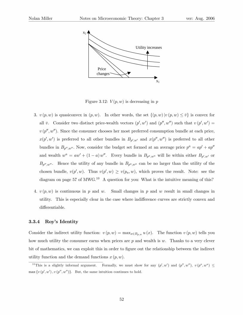
Nolan Miller Notes on Microeconomic Theory: Chapter 3 ver: Aug. 2006
Utility increases
x1
x2
Price changes
Figure 3.12: V (p,w) is decreasing in p
3. v (p,w) is quasiconvex in (p,w). In other words, the set {(p,w) |v (p,w) ≤ v} is convex for
all v. Consider two distinct price-wealth vectors (p0, w0) and (p00, w00) such that v (p0, w0) =
v (p00, w00). Since the consumer chooses her most preferred consumption bundle at each price,
x(p0, w0) is preferred to all other bundles in Bp0,w0 and x(p00, w00) is preferred to all other
bundles in Bp00,w00 . Now, consider the budget set formed at an average price pa = ap0 + ap00
and wealth wa = aw0 + (1− a)w00. Every bundle in Bpa,wa will lie within either Bp0,w0 or
Bp00,w00 . Hence the utility of any bundle in Bpa,wa can be no larger than the utility of the
chosen bundle, v(p0, w). Thus v(p0, w) ≥ v(pa, w), which proves the result. Note: see the
diagram on page 57 of MWG.10 A question for you: What is the intuitive meaning of this?
4. v (p,w) is continuous in p and w. Small changes in p and w result in small changes in
utility. This is especially clear in the case where indifference curves are strictly convex and
differentiable.
3.3.4 Roy’s Identity
Consider the indirect utility function: v (p,w) = maxx∈Bp,w u (x). The function v (p,w) tells you
how much utility the consumer earns when prices are p and wealth is w. Thanks to a very clever
bit of mathematics, we can exploit this in order to figure out the relationship between the indirect
utility function and the demand functions x (p,w).
10This is a slightly informal argument. Formally, we must show for any (p0, w0) and (p00, w00), v (pa, wa) ≤
max {v (p0, w0) , v (p00, w00)}. But, the same intuition continues to hold.
52
Nolan Miller Notes on Microeconomic Theory: Chapter 3 ver: Aug. 2006
The definition of the indirect utility function implies that the following identity is true:
v (p,w) ≡ u (x (p,w)) .
Differentiate both sides with respect to pl :
∂v
∂pl=
LXi=1
∂u
∂xi
∂xi∂pl
.
But, based on the first-order conditions for utility maximization, which we know hold when u () is
evaluated at the optimal x, x (p,w) (see equation (3.1)):
∂u
∂xi= λpi.
And, we also know (from Section 3.3.2) that the Lagrange multiplier is the shadow price of the
constraint: λ = ∂v∂w . Hence:
∂v
∂pl=
LXi=1
∂u
∂xi
∂xi∂pl
=LXi=1
λpi∂xi∂pl
= λLXi=1
pi∂xi∂pl
=∂v
∂w
LXi=1
pi∂xi∂pl
.
Now, recall the comparative statics result of Walras’ Law with respect to a change in pl :
xl (p,w) = −LXi=1
pi∂xi∂pl
.
Substituting this in yields:
∂v
∂pl= − ∂v
∂wxl (p,w)
xl (p,w) = −∂v∂pl∂v∂w
.
The last equation, known as Roy’s identity, allows us to derive the demand functions from the
indirect utility function. This is useful because in many cases it will be easier to estimate an
indirect utility function and derive the direct demand functions via Roy’s identity than to derive
x (p,w) directly. Estimating Roy’s identity involves estimating a single equation. Estimating
x (p,w), on the other hand, amounts to finding for every value of p and w the solution to a set of
L+ 1 first-order equations, which themselves may have unknown parameters.
53

Nolan Miller Notes on Microeconomic Theory: Chapter 3 ver: Aug. 2006
3.3.5 The Indirect Utility Function and Welfare Evaluation
Consider the situation where the price of good 1 increases from p1 to p01. What is the impact
of this price change on the consumer? One way to measure it is in terms of the indirect utility
function:
impact = v¡p0, w
¢− v (p,w) .
That is, the impact of the price change is equal to the difference in the consumer’s utility at prices p0
and p. While this is certainly a measure of the impact of the price change, it is essentially useless.
There are a number of reasons why, but they all hinge on the fact that utility is an ordinal, not a
cardinal concept. As you recall, the only meaning of the numbers assigned to bundles by the utility
function is that x  y if and only if u (x) > u (y). In particular, if u (x) = 2u (y), this does not mean
that the consumer likes bundle x twice as much as bundle y. Also, if u (x)− u (z) > u (s)− u (t),
this doesn’t mean that the consumer would rather switch from bundle z to x than from t to s.
Because of this, there is really nothing we can make of the numerical value of v (p0, w) − v (p,w).
The only thing we can say is that if this difference is positive, the consumer likes (p0, w) more than
(p,w). But, we can’t say how much more.
Another problem with using the change in the indirect utility function as a measure of the
impact of a policy change is that it cannot be compared across consumers. Comparing the change
in two different utility functions is even more meaningless than comparing the change in a single
person’s utility function. This is because even if both utility functions were cardinal measures of
the benefit to a consumer (which they aren’t), there would still be no way to compare the scales
of the two utility functions. This is the “problem of interpersonal comparison of utility,” which
arises in many aspects of welfare economics.
As a possible solution to the problem, consider the following thought experiment. Initially,
prices and wealth are given by (p,w). I am interested in measuring the impact of a change in prices
to p0. So, I ask you the following question: By how much would I have to change your wealth so
that you are indifferent between (p0, w) and (p,w0)? That is, for what value w0 does
v¡p0, w
¢= v
¡p,w0
¢.
The change in wealth, w0 − w, in essence gives a monetary value for the impact of this change in
price. And, this monetary value is a better measure of the impact of the price change than the
utility measurement, because it is, at least to a certain extent, comparable.11 You can compare11 I say to a certain extent, because the value of an additional ∆w dollars of wealth will depend on the initial state.
54

Nolan Miller Notes on Microeconomic Theory: Chapter 3 ver: Aug. 2006
the impact of two different changes in prices by looking at the associated changes in wealth needed
to compensate the consumer. Similarly, you can compare the impact of price changes on different
consumers by comparing the changes in wealth necessary to leave them just as well off.12
Finally, although using the amount of money needed to compensate the consumer is an imperfect
measure of the impact of a policy decision, it has one huge benefit for the neoclassical economist,
and that is that it is observable, at least in principle. There is nothing we can do to observe utility
scales. However, we can often elicit from people the amount of money they would find equivalent
to a certain policy change, either through experiments, surveys, or other estimation techniques.
3.4 The Expenditure Minimization Problem (EMP)
In the previous section, I argued that a good measure of the impact of a change in prices was the
change in wealth necessary to make the consumer as well off at the old prices and new wealth as
she was at the new prices and old wealth. However, this is not an easy exercise when all you have
to work with is the indirect utility function. If we had a function that tells you how much wealth
you would need to have in order to achieve a certain level of utility, then we would be able to do
this much more efficiently. There is such a function. It is called the expenditure function, and
in this section we will develop it.
The expenditure minimization problem (EMP) asks the question, if prices are p, what is
the minimum amount the consumer would have to spend to achieve utility level u? That is:
minx
p · x
s.t. : u (x) ≥ u.
Before we go on, let’s take a moment to figure out what the endogenous and exogenous variables
are here. The exogenous variables are prices p and the reservation (or target) utility level u. The
endogenous variable is x, the consumption bundle. So, in words, the expenditure minimization
bundle amounts to finding the bundle x that minimizes the cost of achieving utility u when prices
are p.
The Lagrangian for this problem is given by:
LEMP = p · x− λ (u (x)− u) .
For instance, poor people presumably value the same wealth increment more than rich people.12Again, this measure is imperfect because it assumes that the two consumers have the same marginal utility of
wealth.
55

Nolan Miller Notes on Microeconomic Theory: Chapter 3 ver: Aug. 2006
Assuming an interior solution, the first-order conditions are given by:13
pi − λui (x) = 0 for i ∈ {1, ..., L} (3.2)
λ (u (x)− u) = 0
If u () is well behaved (e.g., quasiconcave and increasing in each of its arguments), then the con-
straint will bind, and the second condition can be written as u (x) = u. Further, a unique solution
to this problem will exist for any values of p and u. We will denote the value of the solution
to this problem by h (p, u) ∈ X. That is, h (p, u) is an L dimensional vector whose lth compo-
nent, hl (p, u) gives the amount of commodity l that is consumed when the consumer minimizes
the cost of achieving utility u at prices p. The function h (p, u) is known as the Hicksian (or
compensated) demand function.14 It is a demand function because it specifies a consumption
bundle. It differs from the Walrasian (or ordinary) demand function in that it takes p and u as its
arguments, whereas the Walrasian demand function takes p and w as its arguments.
In other words, h (p, u) and x (p,w) are the answers to two different but related problems.
Function x (p,w) answers the question, “Which commodity bundle maximizes utility when prices are
p and wealth is w?” Function h (p, u) answers the question, “Which commodity bundle minimizes
the cost of attaining utility u when prices are p?” We’ll return to the difference between the two
types of demand shortly.
Since h (p, u) solves the EMP, substitution of h (p, u) into the first-order conditions for the EMP
yields the identities (assuming the constraint binds):
pi − λui (h (p, u)) ≡ 0 for i ∈ {1, ..., L}
u (h (p, u))− u ≡ 0
Further, just as we defined the indirect utility function as the value of the objective function of
the UMP, u (x), evaluated at the optimal consumption bundle, x (p,w), we can also define such a
function for the EMP. The expenditure function, denoted e (p, u), is defined by:
e (p, u) ≡ p · h (p, u)
and is equal to the minimum cost of achieving utility u, for any given p and u.
13Again, remember that if f (y) is a function with a vector y as its argument, the notation fi will frequently be
used as shorthand notation for ∂f∂yi. Thus ui denotes ∂u
∂xi.
14We’ll return to why h (p, u) is called the compensated demand function in a while.
56

Nolan Miller Notes on Microeconomic Theory: Chapter 3 ver: Aug. 2006
3.4.1 A First Note on Duality
Consider the first-order conditions (from (3.2)) for xi and xj . Solving each for λ yields:
piui
= λ =pjuj
uiuj
=pipj. (3.3)
Recall that this is the same tangency condition we derived in the UMP. What does this mean?
Consider a price vector p and wealth w. The bundle that solves the UMP, x∗ = x (p,w) is found at
the point of tangency between the budget line and the consumer’s utility isoquant. The consumer’s
utility at this point is given by u∗ = u (x∗). Thus x∗ is the point of tangency between the line
p · x = w and the curve u (x) = x∗.
Now, consider the EMP when the target utility level is given by u∗. The bundle that solves
the EMP is the bundle that achieves utility u∗ at minimum cost. This is located by finding the
point of tangency between the curve u (x) = u∗ and a budget line (which is what (3.3) says). But,
we already know from the UMP that the curve u (x) = u∗ is tangent to the budget line p · x = w
at x∗ (and is tangent to no other budget line). Hence x∗ must solve the EMP problem when the
target utility level is u∗! Further, since x∗ lies on the budget line, p · x∗ = w. So the minimum
cost of achieving utility u∗ is w. Thus the UMP and the EMP pick out the same point.
Let me restate what I’ve just argued. If x∗ solves the UMP when prices are p and wealth is w,
then x∗ solves the EMP when prices are p and the target utility level is u (x∗). Further, maximal
utility in the UMP is u (x∗) and minimum expenditure in the EMP is w. This result is called the
“duality” of the EMP and the UMP.
The UMP and the EMP are considered dual problems because the constraint in the UMP is
the objective function in the EMP and vice versa. This is illustrated by looking at the graphical
solutions to the two problems. In the UMP, shown in Figure 3.13, you keep increasing utility until
you find the one that is tangent to the budget line.In the EMP, on the other hand, shown in Figure
3.14, you keep decreasing expenditure (which is like shifting a budget line toward the origin) until
you find the expenditure line that is tangent to u (x) = u∗. Although the process of finding the
optimal point is different in the UMP and EMP, they both pick out the same point because they
are looking for the same basic relationship, as expressed in equation (3.3).
The duality relationship between the EMP and the UMP is captured by the following identities,
57

Nolan Miller Notes on Microeconomic Theory: Chapter 3 ver: Aug. 2006
x*
p1x1 + p2x2 = w
u(x)=u*
Figure 3.13: The Utility Maximization Problem
x*
p1x1 + p2x2 = w
u(x)=u*
Figure 3.14: The Expenditure Minimization Problem
58

Nolan Miller Notes on Microeconomic Theory: Chapter 3 ver: Aug. 2006
to which we will return later:
h (p, v (p,w)) ≡ x (p,w)
x (p, e (p, u)) ≡ h (p, u) .
These identities restate the principles discussed previously. The first says that the commodity
bundle that minimizes the cost of achieving the maximum utility you can achieve when prices are
p and wealth is w is the bundle that maximizes utility when prices are p and wealth is w. The
second says that the bundle that maximizes utility when prices are p and wealth is equal to the
minimum amount of wealth needed to achieve utility u at those prices is the same as the bundle
that minimizes the cost of achieving utility u when prices are p.
Similar identities can be written using the indirect utility function and expenditure function:
u ≡ v (p, e (p, u))
w ≡ e (p, v (p,w)) .
Note to MWG readers: There is a mistake in Figure 3.G.3. The relationships on
the horizontal line connecting v (p,w) and e (p, u) should be the ones written directly
above.
The main implication of the previous analysis is this: The expenditure function contains the
exact same information as the indirect utility function. And, since the indirect utility function can
be used (by Roy’s identity) to derive the Walrasian demand functions, which can, in turn, be used
to recover preferences, the expenditure function contains the exact same information as
the utility function. This means that if you know the consumer’s expenditure function, you
know her utility function, and vice versa. No information is lost along the way. This is another
expression of what people mean when they say that the UMP and EMP are dual problems - they
contain exactly the same information.
3.4.2 Properties of the Hicksian Demand Functions and Expenditure Function
In this section, we refer both to function u (x) and to a particular level of utility, u. In order to be
clear, let’s put a bar over the u when we are talking about a level of utility, i.e., u. Just as we derived
the properties of x (p,w) and v (p,w), we can also derive the properties of the Hicksian demand
functions h (p, u) and expenditure function e (p, u). Let’s begin with h (p, u) . We will assume that
u () is a continuous utility function representing a locally non-satiated preference relation.
59

Nolan Miller Notes on Microeconomic Theory: Chapter 3 ver: Aug. 2006
Properties of the Hicksian Demand Functions
The Hicksian demand functions have the following properties:
1. Homogeneity of degree zero in p : h (αp, u) ≡ h (p, u) for p, u, and α > 0. NOTE: THIS IS
HOMOGENEITY IN P , NOT HOMOGENEITY IN P AND U ! Homogeneity of degree zero
is best understood in terms of the graphical presentation of the EMP. The solution to the
EMP is the point of tangency between the utility isoquant u (x) = u and one of the budget
lines. This is determined by the slope of the expenditure lines (lines of the form p · x = k,
where k is any constant). Any change that doesn’t affect the slope of the budget lines should
not affect the cost-minimizing bundle (although it will affect the expenditure on the cost
minimizing bundle). Since the slope of the expenditure line is determined by relative prices
and since scaling all prices by the same amount does not affect relative prices, the solution
should not change. More formally, the EMP at prices αp is
minx
αp · x
s.t. : u (x) ≥ u.
But, this problem is formally equivalent to:
minα (p · x) : s.t. : u (x) ≥ x
which is equivalent to:
αminx
p · x : s.t. : u (x) ≥ x
which is just the same as the EMP when prices are p, except that total expenditure is
multiplied by α, which doesn’t affect the cost minimizing bundle.
2. No excess utility: u (h (p, u)) = u. This follows from the continuity of u (). Suppose
u (h (p, u)) > u. Then consider a bundle h0 that is slightly smaller than h (p, u) on all
dimensions. By continuity, if h0 is sufficiently close to h (p, u), then u (h0) > u as well. But,
then h0 is a bundle that achieves utility u at lower cost than h (p, u), which contradicts the
assumption that h (p, u) was the cost minimizing bundle in the first place.15 From this we
can conclude that the constraint always binds in the EMP.15This type of argument - called “Proof by Contradiction” - is quite common in economics. If you want to show
a implies b, assume that b is false and show that if b is false then a must be false as well. Since a is assumed to be
true, this implies that b must be true as well.
60

Nolan Miller Notes on Microeconomic Theory: Chapter 3 ver: Aug. 2006
3. If preferences are convex, then h (p, u) is a convex set. If preferences are strictly convex (i.e.
u () is strictly quasiconcave), then h (p, u) is single valued.
Properties of the Expenditure Function
Based on the properties of h (p, u), we can derive properties of the expenditure function, e (p, u).
1. Function e (p, u) is homogeneous of degree one in p: Since h (p, u) is homogeneous of
degree zero in p, this means that scaling all prices by α > 0 does not affect the bundle
demanded. Applying this to total expenditure:
e (αp, u) = αp · h (αp, u) = αp · h (p, u) = αe (p, u) .
In words, if all prices change by a factor of α, the same bundle as before achieves utility level
u at minimum cost, only it now costs you twice as much as it used to. This is exactly what
it means for a function to be homogeneous of degree one.
2. Function e (p, u) is strictly increasing in u and non-decreasing in pl for any l. I’ll
give the argument here to show that e (p, u) cannot be decreasing in u. There are a few
more details to show that it cannot stay constant either, but most of the intuition of the
argument is contained in showing that e (p, u) cannot be strictly decreasing. The argu-
ment is by contradiction. Suppose that for u0 > u, e (p, u) > e (p, u0). But, then h (p, u0)
satisfies the constraint u (x) ≥ u and does so at lower cost than h (p, u), which contra-
dicts the assumption that h (p, u) is the cost minimizing bundle that achieves utility level u.
The argument that e (p, u) is nondecreasing in pl uses another method which is quite common,
a method I call “feasible but not optimal.” Let p and p0 differ only in component l, and let
p0l > pl. From the definition of the expenditure function, e (p0, u) = p0 ·h (p0, u) ≥ p·h (p0, u) ≥
e (p, u). The first equality follows from the definition of the expenditure function, the first
≥ follows from the fact that p0 > p (note: p0 · h (p0, u) > p · h (p, u) if hl (p0, u) > 0), and the
second ≥ follows from the fact that h (p0, u) achieves utility level u but does not necessarily
do so at minimum cost (i.e. h (p0, u) is feasible in the EMP for (p, u) but not necessarily
optimal).
3. Function e (p, u) is concave in p.16 Consider two price vectors p and p0, and let pa =
16Recall the definition of concavity. Consider y and y0 such that y 6= y0. Function f (y) is concave if, for any
a ∈ [0, 1], f (ay + (1− a) y0) ≥ af (y) + (1− a) f (y0).
61

Nolan Miller Notes on Microeconomic Theory: Chapter 3 ver: Aug. 2006
ap+ (1− a) p0.
e (pa, u) = pa · h (pa, u)
= ap · h (pa, u) + (1− a) p · h (pa, u)
≥ ap · h (p, u) + (1− a) p0 · h¡p0, u
¢where the first line is the definition of e (p, u), the second follows from the definition of pa,
and the third follows from the fact that h (pa, u) is feasible but not optimal in the EMP for
(p, u) and (p0, u).
The following heuristic explanation is also helpful in understanding the concavity of e (p, u).
Suppose prices change from p to p0. If the consumer continued to consume the same bundle at the
old prices, expenditure would increase linearly:
∆expenditure =¡p0 − p
¢· h (p, u) .
But, in general the consumer will not continue to consume the same bundle after the price change.
Rather, he will rearrange his bundle in order to minimize the cost of achieving u at the new prices,
p0. Since this will save the consumer some money, total expenditure will decrease at less than a
linear rate. And, an alternate definition of concavity is that the function always increases at less
than a linear rate. In other words, f (x) is concave if it always lies below its tangent lines.17
3.4.3 The Relationship Between the Expenditure Function and Hicksian De-
mand
Just as there was a relationship between the indirect utility function v (p,w) and the Walrasian
demand functions x (p,w), there is also a relationship between the expenditure function e (p, u)
and the Hicksian demand function h (p, u). In fact, it is even more straightforward for e (p, u) and
h (p, u). Let’s start with the derivation
e (p, u) ≡ p · h (p, u)
Since this is an identity, differentiate it with respect to pi:
∂e
∂pi≡ hi (p, u) +
Xj
pj∂hj∂pi
.
17This explanation will be clearer once we show that hl (p, u) =∂e(p,u)∂pl
, i.e. that hl (p, u) is exactly the rate of
increase in expenditure if pl increases by a small amount. Thus e (p0, u)− e (p, u) ≤ h (p, u) · (p0 − p) is exactly the
definition of concavity.
62

Nolan Miller Notes on Microeconomic Theory: Chapter 3 ver: Aug. 2006
Now, substitute in the first-order conditions, pj = λuj
∂e
∂pi≡ hi (p, u) + λ
Xj
uj∂hj∂pi
. (3.4)
Since the constraint binds at any optimum of the EMP,
u (h (p, u)) ≡ u
Differentiate with respect to pi : Xj
uj∂hj∂pi
= 0
and substituting this into (3.4) yields:
∂e
∂pj≡ hj (p, u) . (3.5)
That is, the derivative of the expenditure function with respect to pj is just the Hicksian demand
for commodity j.
The importance of this result is similar to the importance of Roy’s identity. Frequently, it
will be easier to measure the expenditure function than the Hicksian demand function. Since
we are able to derive the Hicksian demand function from the expenditure function, we can derive
something that is hard to observe from something that is easier to observe.
From (3.5) we can derive several additional properties (assuming u () is strictly quasiconcave
and h () is differentiable):
1. (a) ∂hi∂pj
= ∂2e∂pi∂pj
. This one follows directly from the fact that (3.5) is an identity. Let
Dph (p, u) be the matrix whose ith row and jth column is ∂hi∂pj. This property is thus
the same as saying that Dph (p, u) ≡ D2pe (p, u), where D
2pe (p, u) is the matrix of second
derivatives (Hessian matrix) of e (p, u).
(b) Dph (p, u) is a negative semi-definite (n.s.d.) matrix. This follows from the fact that
e (p, u) is concave, and concave functions have Hessian matrices that are n.s.d. The
main implication is that the diagonal elements are non-positive, i.e., ∂hi∂pi≤ 0.
(c) Dph (p, u) is symmetric. This follows from Young’s Theorem (that it doesn’t matter
what order you take derivatives in): ∂hi∂pj
= ∂2e∂pi∂pj
=∂hj∂pi. The implication is that the
cross-effects are the same — the effect of increasing pj on hi is the same as the effect of
increasing pi on hj .
63

Nolan Miller Notes on Microeconomic Theory: Chapter 3 ver: Aug. 2006
x
x'
p
p'
Figure 3.15: Compensated Demand
(d)P
j∂hi∂pj
pj = 0 for all i . This follows from the homogeneity of degree zero of h (p, u) in
p. Consider the identity:
h (ap, u) ≡ h (p, u) .
Differentiate with respect to a and evaluate at a = 1, and you have this result.
The Hicksian demand curve is also known as the compensated demand curve. The reason
for this is that implicit in the definition of the Hicksian demand curve is the idea that following a
price change, you will be given enough wealth to maintain the same utility level you did before the
price change. So, suppose at prices p you achieve utility level u. The change in Hicksian demand
for good i following a change to prices p0 is depicted in Figure 3.15.
When prices are p, the consumer demands bundle x, which has total expenditure p · x = w.
When prices are p0, the consumer demands bundle x0, which has total expenditure p0 · x0 = w0.
Thus implicit in the definition of the Hicksian demand curve is the idea that when prices change
from p to p0, the consumer is compensated by changing wealth from w to w0 so that she is exactly
as well off in utility terms after the price change as she was before.
Note that since ∂hi∂pi≤ 0, this is another statement of the compensated law of demand (CLD).
When the price of a good goes up and the consumer is compensated for the price change, she will
not consume more of the good. The difference between this version and the previous version we
saw (in the choice based approach) is that here, the compensation is such that the consumer can
achieve the same utility before and after the price change (this is known as Hicksian substitution),
and in the previous version of the CLD the consumer was compensated so that she could just afford
the same bundle as she did before (this is known as Slutsky compensation). It turns out that the
64

Nolan Miller Notes on Microeconomic Theory: Chapter 3 ver: Aug. 2006
two types of compensation yield very similar results, and, in fact, for differential changes in price,
they are identical.
3.4.4 The Slutsky Equation
Recall that the whole point of the EMP was to generate concepts that we could use to evaluate
welfare changes. The purpose of the expenditure function was to give us a way to measure the
impact of a price change in dollar terms. While the expenditure function does do this (you can just
look at e (p0, u)− e (p, u)), it suffers from another problem. The expenditure function is based on
the Hicksian demand function, and the Hicksian demand function takes as its arguments prices and
the target utility level u. The problem is that while prices are observable, utility levels certainly
are not. And, while we can generate some information by asking people over and over again how
they compare certain bundles, this is not a very good way of doing welfare comparisons.
To summarize our problem: The Walrasian demand functions are based on observables (p,w)
but cannot be used for welfare comparisons. The Hicksian demand functions, on the other hand,
can be used to make welfare comparisons, but are based on unobservables.
The solution to this problem is to somehow derive h (p, u) from x (p,w). Then we could use our
observations of p and w to derive h (p, u), and use h (p, u) for welfare evaluation. Fortunately, we
can do exactly this. Suppose that u (x (p,w)) = u (which implies that e (p, u) = w), and consider
the identity:
hi (p, u) ≡ xi (p, e (p, u)) .
Differentiate both sides with respect to pj :
∂hi∂pj
≡ ∂xi (p, e (p, u))
∂pj+
∂xi (p, e (p, u))
∂e(p, u)
∂e (p, u)
∂pj
≡ ∂xi (p,w)
∂pj+
∂xi (p,w)
∂whj (p, u)
≡ ∂xi (p,w)
∂pj+
∂xi (p,w)
∂wxj (p, e (p, u))
≡ ∂xi (p,w)
∂pj+
∂xi (p,w)
∂wxj (p,w) .
The equation∂hi (p, v (p,w))
∂pj≡ ∂xi (p,w)
∂pj+
∂xi (p,w)
∂wxj (p,w)
is known as the Slutsky equation. Note that it provides the link between the Walrasian demand
functions x (p,w) and the Hicksian demand functions, h (p, u). Thus if we estimate the right-hand
65

Nolan Miller Notes on Microeconomic Theory: Chapter 3 ver: Aug. 2006
side of this equation, which is a function of the observables p and w, then we can derive the value
of the left-hand side of the equation, even though it is based on unobservable u.
Recall that implicit in the idea of the Hicksian demand function is the idea that the consumer’s
wealth would be adjusted so that she can achieve the same utility after a price change as she did
before. This idea is apparent when we look at the Slutsky equation. It says that the change in
demand when the consumer’s wealth is adjusted so that she is as well off after the change as she
was before is made up of two parts. The first, ∂xi(p,w)∂pj
, is equal to how much the consumer would
change demand if wealth were held constant. The second, ∂xi(p,w)∂w xi (p,w), is the additional change
in demand following the compensation in wealth.
For example, consider an increase in the price of gasoline. If the price of gasoline goes up by
one unit, consumers will tend to consume less of it, if their wealth is held constant (since it is not
a Giffen good). However, the fact that gasoline has become more expensive means that they will
have to spend more in order to achieve the same utility level. The amount by which they will
have to be compensated is equal to the change in price multiplied by the amount of gasoline the
consumer buys, xi (p,w). However, when the consumer is given xi (p,w) more units of wealth to
spend, she will adjust her consumption of gasoline further. Since gasoline is normal, the consumer
will increase her consumption. Thus the compensated change in demand (sometimes called the
pure substitution effect), ∂hi(p,v(p,w))∂pj, will be the sum of the uncompensated change (also known
as the substitution effect), ∂xi(p,w)∂pj
, and the wealth effect, ∂xi(p,w)∂w xi (p,w).18
In order to make this clear, let’s rearrange the Slutsky equation and go through the intuition
again.∂xi (p,w)
∂pj≡ ∂hi (p, v (p,w))
∂pj− ∂xi (p,w)
∂wxj (p,w)
Here, we are interested in explaining an uncompensated change in demand in terms of the compen-
sated change and the wealth effect. Think about the effect of an increase in the price of bananas on
a consumer’s Walrasian demand for bananas. If the price of bananas were to go up, and my wealth
were adjusted so that I could achieve the same amount of utility before and after the change, I would
consume fewer bananas. This follows directly from the CLD: ∂hi∂pi≤ 0. However, the change in
compensated demand assumes that the consumer will be compensated for the price change. Since
an increase in the price of bananas is a bad thing, this means that ∂hi∂pi
has built into it the idea
18This latter term is often called the “income effect,” which is not quite right. Variable w stands for total wealth,
which is more than just income. When people call this the income effect (as I sometimes do), they are just being
sloppy.
66

Nolan Miller Notes on Microeconomic Theory: Chapter 3 ver: Aug. 2006
that income will be increased in order to compensate the consumer. But, in reality consumers are
not compensated for price changes, so we are interested in the uncompensated change in demand∂xi∂pi. This means that we must remove from the compensated change in demand the effect of the
compensation. Since ∂hi∂pi
assumed an increase in wealth, we must impose a decrease in wealth,
which is just what the terms −∂xi(p,w)∂w xi (p,w) are. The decrease in wealth is given by −xi (p,w),
and the effect of this decrease on demand for bananas is given by ∂xi∂w .
19
3.4.5 Graphical Relationship of the Walrasian and Hicksian Demand Functions
Demand functions are ordinarily graphed with price on the vertical axis and quantity on the hor-
izontal axis, even though this is technically “backward.” But, we will follow with tradition and
draw our graphs this way as well.
The difference between the compensated demand response to a price change and the uncom-
pensated demand response to a price change is equal to the wealth effect:
∂hi (p, v (p,w))
∂pj≡ ∂xi (p,w)
∂pj+
∂xi (p,w)
∂wxj (p,w)
Since ∂hi∂pj
is negative, when the wealth effect is positive (i.e., good i is normal) this means that the
Hicksian demand curve will be steeper than the Walrasian demand curve at any point where they
cross.20 If, on the other hand, the wealth effect is negative (i.e. good i is inferior), this means that
the Hicksian demand curve will be less steep than the Walrasian demand curve (see MWG Figure
3.G.1).
Let’s go into a bit more detail in working out the relative slopes of the Walrasian and Hicksian
demand curves and determining how changes in u shift the Hicksian demand curve (depending on
whether the good is normal or inferior).
In this subsection we discuss how changes in the exogenous parameters, p and u, affect the
Hicksian Demand curve when it is drawn on the typical P -Q axes.
19We are interested in the total change in consumption of bananas when the price of bananas goes up. In the
real world, we don’t compensate people when prices change. But, the Slutsky equation tells us that the total
(uncompensated) effect of a change in the price of bananas is a combination of the substitution effect (compensated
effect) and the wealth effect. This result should be familiar to you from your intermediate micro course. If it
isn’t, you may want to take a look at the (less abstract) treatment of this point in an intermediate micro text, such
as Varian’s Intermediate Microeconomics. Test of understanding: If bananas are a normal good, could demand for
bananas ever rise when the price increases (i.e. could bananas be a Giffen good)? Answer using the Slutsky equation.20Remember that the graphs are backwards, so a less negative slope ∂hi
∂pjis actually steeper.
67

Nolan Miller Notes on Microeconomic Theory: Chapter 3 ver: Aug. 2006
Part 0: Recall that ∂hi∂pi≤ 0 because the Slutsky matrix is negative semi-definite. We’ll
assume, as is typical, that ∂hi∂pi
< 0. To keep things simple, I’ll omit the subscripts for the rest of
the subsection, since we’re always talk about a single good.
Part 1: Relationship between Hicksian and Walrasian Demand.
By duality, we know that through any point on Walrasian demand there is a Hicksian demand
curve through that point. How do their slopes compare? This is given by the Slutsky equation.
But, keep in mind two things. First, since we put p on the vertical axis and x on the horizontal
axis, when we draw a graph, the derivatives of the demand functions aren’t slopes. They’re inverse
slopes. That is, the slope of the Walrasian demand is 1∂x/∂p and the slope of the Hicksian is
1∂h/∂p .
Second, these derivatives are usually negative. So, we have to be a bit careful about thinking about
quantities that are larger (i.e., further to the right on the number line) and quantities that are
larger in magnitude (i.e., are further from zero on the number line). Since slopes are negative, a
“larger” slope corresponds to a flatter curve. You’lls ee why this is important in a minute.
To figure out whether x (p,w) or h (p, u) through a point is steeper, use the Slutsky equation.
∂h
∂p=
∂x
∂p+
∂x
∂wx.
The answer will depend on whether x is normal or inferior. So, begin by considering a normal
good. In this case, ∂x∂px > 0, so:
∂h
∂p>
∂x
∂p¯∂h
∂p
¯<
¯∂x
∂p
¯1¯∂h∂p
¯ >1¯∂x∂p
¯The first line comes from the Slutsky equation and the fact that the income effect is positive. The
second comes from the fact that, for a normal good, both sides are negative, and hence if ∂h∂p > ∂x
∂p ,
∂h∂p is smaller in magnitude (absolute value) than
∂x∂p . The third follows from the second sinxe if
x < y and both are positve, then 1/x > 1/y. Hence, for normal goods, the Hicksian Demand
through a point is steeper than the Walrasian Demand through that point.
For an inferior good, things reverse. To simplify, suppose x is inferior but not Giffen (so that
68
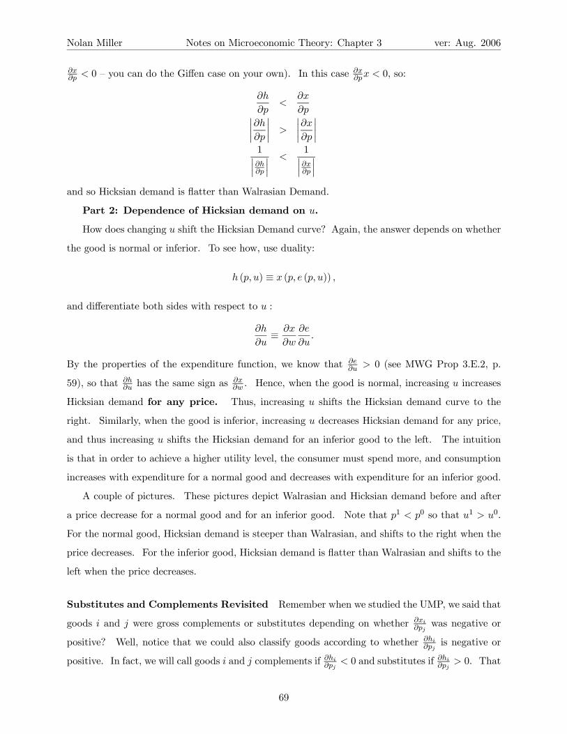
Nolan Miller Notes on Microeconomic Theory: Chapter 3 ver: Aug. 2006
∂x∂p < 0 — you can do the Giffen case on your own). In this case ∂x
∂px < 0, so:
∂h
∂p<
∂x
∂p¯∂h
∂p
¯>
¯∂x
∂p
¯1¯∂h∂p
¯ <1¯∂x∂p
¯and so Hicksian demand is flatter than Walrasian Demand.
Part 2: Dependence of Hicksian demand on u.
How does changing u shift the Hicksian Demand curve? Again, the answer depends on whether
the good is normal or inferior. To see how, use duality:
h (p, u) ≡ x (p, e (p, u)) ,
and differentiate both sides with respect to u :
∂h
∂u≡ ∂x
∂w
∂e
∂u.
By the properties of the expenditure function, we know that ∂e∂u > 0 (see MWG Prop 3.E.2, p.
59), so that ∂h∂u has the same sign as
∂x∂w . Hence, when the good is normal, increasing u increases
Hicksian demand for any price. Thus, increasing u shifts the Hicksian demand curve to the
right. Similarly, when the good is inferior, increasing u decreases Hicksian demand for any price,
and thus increasing u shifts the Hicksian demand for an inferior good to the left. The intuition
is that in order to achieve a higher utility level, the consumer must spend more, and consumption
increases with expenditure for a normal good and decreases with expenditure for an inferior good.
A couple of pictures. These pictures depict Walrasian and Hicksian demand before and after
a price decrease for a normal good and for an inferior good. Note that p1 < p0 so that u1 > u0.
For the normal good, Hicksian demand is steeper than Walrasian, and shifts to the right when the
price decreases. For the inferior good, Hicksian demand is flatter than Walrasian and shifts to the
left when the price decreases.
Substitutes and Complements Revisited Remember when we studied the UMP, we said that
goods i and j were gross complements or substitutes depending on whether ∂xi∂pj
was negative or
positive? Well, notice that we could also classify goods according to whether ∂hi∂pj
is negative or
positive. In fact, we will call goods i and j complements if ∂hi∂pj< 0 and substitutes if ∂hi∂pj
> 0. That
69
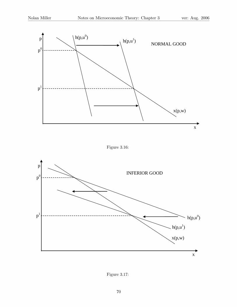
Nolan Miller Notes on Microeconomic Theory: Chapter 3 ver: Aug. 2006
p
x
x(p,w)
h(p,u1) h(p,u0)
p0
p1
NORMAL GOOD
Figure 3.16:
p
x
x(p,w)
h(p,u1)
h(p,u0)
p0
p1
INFERIOR GOOD
Figure 3.17:
70

Nolan Miller Notes on Microeconomic Theory: Chapter 3 ver: Aug. 2006
is, we drop the “gross” when talking about the Hicksian demand function.21 In many ways, the
Hicksian demand function is the proper function to use to talk about substitutes and complements
since it separates the question of wealth effects and substitution effects. For example, it is possible
that good j is a gross complement for good i while good i is a gross substitute for good j (if good
i is normal and good j is inferior), but no such thing is possible when talking about (just plain)
complements or substitutes since ∂hi∂pj
=∂hj∂pi.
3.4.6 The EMP and the UMP: Summary of Relationships
The relationships between all of the parts of the EMP and the UMP are summarized in Figure
3.G.3 of MWG and similar figures appear in almost any other micro theory book. So, I urge you
to look it over (with the proviso about the typo that I mentioned earlier).
Here, I’ll do it in words. Start with the UMP.
maxu (x)
s.t : p · x ≤ w.
The solution to this problem is x (p,w), the Walrasian demand functions. Substituting x (p,w)
into u (x) gives the indirect utility function v (p,w) ≡ u (x (p,w)). By differentiating v (p,w) with
respect to pi and w, we get Roy’s identity, xi (p,w) ≡ −vpivw
.
Now the EMP.
min p · x
s.t. : u (x) ≥ u.
The solution to this problem is the Hicksian demand function h (p, u), and the expenditure function
is defined as e (p, u) ≡ p · h (p, u). Differentiating the expenditure function with respect to pj gets
you back to the Hicksian demand, hj (p, u) ≡ ∂e(p,u)∂pj
.
The connections between the two problems are provided by the duality results. Since the same
bundle that solves the UMP when prices are p and wealth is w solves the EMP when prices are p
and the target utility level is v (p,w), we have that
x (p,w) ≡ h (p, v (p,w))
h (p, u) ≡ x (p, e (p, u)) .
21You can think of the ‘gross’ as referring to the fact that ∂xi∂pj
captures the effect of the price change before adding
in the effect of compensation, sort of like how gross income is sales before adding in the effect of expenses.
71

Nolan Miller Notes on Microeconomic Theory: Chapter 3 ver: Aug. 2006
Applying these identities to the expenditure and indirect utility functions yields more identities:
v (p, e (p, u)) ≡ u
e (p, v (p,w)) ≡ w.
Note: These last equations are where the mistake is in the book. Finally, from the relationship
between x (p,w) and h (p, u) we can derive the Slutsky equation:
∂hi (p, v (p,w))
∂pj≡ ∂xi (p,w)
∂pj+
∂xi (p,w)
∂wxj .
If you are really interested in such things, there is also a way to recover the utility function from
the expenditure function (see a topic in MWG called “integrability”), but I’m not going to go into
that here.
3.4.7 Welfare Evaluation
Underlying our approach to the study of preferences has been the ultimate goal of developing a
tool for the welfare evaluation of policy changes. Recall that:
1. The UMP leads to x (p,w) and v (p,w), which are at least in principle observable. However,
v (p,w) is not a good tool for welfare analysis.
2. The EMP leads to h (p, u) and e (p, u), which are based on unobservables (u) but provide a
good measure for the change in a consumer’s welfare following a policy change.
3. The Slutsky equation provides the link between the observable concepts, x (p,w), and the
useful concepts, h (p, u).
In this section, we explore how these tools can be used for welfare analysis. The neoclassical
preference-based approach to consumer theory gives us a measure of consumer well-being, both in
terms of utility and in terms of the wealth needed to achieve a certain level of well-being. It turns
out that this is crucial for welfare evaluation.
We will consider a consumer with “well-behaved” preferences (i.e. a strictly increasing, strictly
quasiconcave utility function). The example we will focus on is the welfare impact of a price
change.
Consider a consumer who has wealth w and faces initial prices p0. Utility at this point is given
by
v¡p0, w
¢.
72
Nolan Miller Notes on Microeconomic Theory: Chapter 3 ver: Aug. 2006
If prices change to p1, the consumer’s utility at the new prices is given by:
v¡p1, w
¢.
Thus the consumer’s utility increases, stays constant, or decreases depending on whether:
v¡p1, w
¢− v
¡p0, w
¢is positive, equal to zero, or negative.
While looking at the change in utility can tell you whether the consumer is better off or not, it
cannot tell you how much better off the consumer is made. This is because utility is an ordinal
concept. The units that utility is measured in are arbitrary. Thus it is meaningless to compare,
for example, v¡p1, w
¢− v
¡p0, w
¢and v (p2, w) − v (p3, w). And, if v () and y () are the indirect
utility functions of two people, it is also meaningless to compare the change in v to the change in
y.
However, suppose we were to compare, instead of the direct utility earned at a particular price-
wealth pair, the wealth needed to achieve a certain level of utility at a given price-wealth pair. To
see how this works, let
u1 = v¡p1, w
¢u0 = v
¡p0, w
¢.
We are interested in comparing the expenditure needed to achieve u1 or u0. Of course, this
will depend on the particular prices we use. It turns out that we have broad latitude to choose
whichever set of prices we want, so let’s call the reference price vector pref , and we’ll assume that
it is strictly greater than zero on all components.
The expenditure needed to achieve utility level u at prices pref is just
e³pref , u
´.
Thus, if we want to compare the expenditure needed to achieve utility u0 and u1, this is given
by:
e³pref , u1
´− e
³pref , u0
´e³pref , v
¡p1, w
¢´− e
³pref , v
¡p0, w
¢´.
This expression will be positive whenever it takes more wealth to achieve utility u1 at prices pref
than to achieve u0. Hence this expression will also be positive, zero, or negative depending on
73

Nolan Miller Notes on Microeconomic Theory: Chapter 3 ver: Aug. 2006
whether u1 > u0, u1 = u0, or u1 < u0. However, the units now have meaning. The difference
is measured in dollar terms. Because of this, e¡pref , v (p,w)
¢is often called a money metric
indirect utility function.
We can construct a money metric indirect utility function using virtually any strictly positive
price as the reference price pref . However, there are two natural candidates: the original price,
p0, and the new price, p1. When pref = p0, the change in expenditure is equal to the change in
wealth such that the consumer would be indifferent between the new price with the old wealth and
the old price with the new wealth. Thus it asks what change in wealth would be equivalent to the
change in price. Formally, define the equivalent variation, EV¡p0, p1, w
¢, as
EV¡p0, p1, w
¢= e
¡p0, v
¡p1, w
¢¢− e
¡p0, v
¡p0, w
¢¢= e
¡p0, v
¡p1, w
¢¢− w.
since e¡p0, v
¡p0, w
¢¢= w. Equivalent variation is illustrated in MWG Figure 3.I.2, panel a. Notice
that the compensation takes place at the old prices — the budget line shifts parallel to the one for¡p0, w
¢.
Since w = e¡p1, v
¡p1, w
¢¢, an alternative definition of EV would be:
EV¡p0, p1, w
¢= e
¡p0, v
¡p1, w
¢¢− e
¡p1, v
¡p1, w
¢¢.
In this form, EV asks how much more money does it take to achieve utility level v¡p1, w
¢at p0
than at p1. Note: if EV < 0, this means that it takes less money to achieve utility v¡p1, w
¢at p0
than p1 (which means that prices have gone up to get to p1, at least on average).
When considering the case where the price of only one good changes, EV has a useful interpre-
tation in terms of the Hicksian demand curve. Applying the fundamental theorem of calculus and
the fact that ∂e(p,u)∂pi
= hi (p, u), if only the price of good 1 changes, we have:22
e¡p0, v
¡p1, w
¢¢− e
¡p1, v
¡p1, w
¢¢=
Z p01
p11
h1¡s, p0−1, v
¡p1, w
¢¢ds
Thus the absolute value of EV is given by the area to the left of the Hicksian demand curve between
p01 and p11. If p01 < p11, EV is negative - a welfare loss because prices went up. If p01 > p11, EV is
22Often when we are interested in a particular component of a vector - say, the price of good i - we will write the
vector as (pi, p−i), where p−i consists of all the other components of the price vector. Thus, (p∗i , p−i) stands for the
vector (p1, p2, ..., pi−1, p∗i , pi+1, ..., pL). It’s just a shorthand notation.
Another notational explanation - in an expression such as p01, the superscript refers to the timing of the price vector
(i.e. new or old prices), and the subscript refers to the commodity. Thus, p01 is the old price of good 1.
74
Nolan Miller Notes on Microeconomic Theory: Chapter 3 ver: Aug. 2006
positive - a welfare gain because prices went down. The relevant area is depicted in MWG Figure
3.I.3, panel a.
The other case to consider is the one where the new price is taken as the reference price. When
pref = p1, the change in expenditure is equal to the change in wealth such that the consumer is
indifferent between the original situation¡p0, w
¢and the new situation (p1, w+∆w). Thus it asks
how much wealth would be needed to compensate the consumer for the price change. Formally,
define the compensating variation (depicted in MWG Figure 3.I.2, panel b)
CV¡p0, p1, w
¢= e
¡p1, v
¡p1, w
¢¢− e
¡p1, v
¡p0, w
¢¢= w − e
¡p1, v
¡p0, w
¢¢.
Again, when only one price changes, we can readily interpret CV in terms of the area to the
left of a Hicksian demand curve. However, this time it is the Hicksian demand curve for the old
utility level, u0. To see why, note that w = e¡p0, v
¡p0, w
¢¢, and so (again assuming only the price
of good 1 changes):
CV¡p0, p1, w
¢= e
¡p0, v
¡p0, w
¢¢− e
¡p1, v
¡p0, w
¢¢=
Z p01
p11
h1¡s, p0−1, v
¡p0, w
¢¢ds,
which is positive whenever p01 > p11 and negative whenever p01 < p11. The relevant area is illustrated
in MWG Figure 3.I.3, panel b.
Recall that whenever good i is a normal good, increasing the target utility level u shifts
hi (pi, p−i, u) to the right in the (xi, pi) space. This is because in order to achieve higher utility the
consumer will need to spend more wealth, and if the good is normal and the consumer spends more
wealth, more of the good will be consumed. Thus when the good is normal, EV ≥ CV . On the
other hand, if the good is inferior, then increasing u shifts hi (pi, p−i, u) to the left, and CV ≥ EV .
When there is no wealth effect on the good, i.e., ∂xi(p,w)∂w = 0, then CV = EV.
Figure 3.I.3 also shows theWalrasian demand curve. In fact, it shows it crossing h¡p1, p
0−1, v
¡p1, w
¢¢at p11 and h1
¡p1, p
0−1, v
¡p0, w
¢¢at p01. This results from the duality of utility maximization and
expenditure minimization. Formally, we have the equalities
h1¡p0, v
¡p0, w
¢¢= x
¡p0, w
¢h1¡p1, v
¡p1, w
¢¢= x
¡p1, w
¢,
which each arise from the identity hi (p, v (p,w)) ≡ xi (p,w). The result of this is that the Walrasian
demand curve crosses the Hicksian demand curves at the two points mentioned above, and that
the area to the left of the Walrasian demand curve lies somewhere between the EV and CV. There
are a number of comments that must be made on this topic:
75

Nolan Miller Notes on Microeconomic Theory: Chapter 3 ver: Aug. 2006
1. Although the area to the left of the Hicksian demand curve is equal to the change in the
expenditure function, the area to the left of the Walrasian demand function has no ready
interpretation.
2. The area to the left of the Walrasian demand curve is called the change in Marshallian
consumer surplus, ∆CS, and is probably the notion of welfare change that you are used to
from your intermediate micro courses.
3. Unfortunately, the change in Marshallian consumer surplus is a meaningless measure (see
part 1) except for:
(a) If there are no wealth effects on the good whose price changes, then EV = CV = ∆CS.
(b) Since ∆CS lies between EV and CV , it can sometimes be a good approximation of the
welfare impact of a price change. This is especially true if wealth effects are small.
4. Some might argue that ∆CS is a useful concept because it is easier to compute than EV or
CV since it does not require estimation of the Hicksian demand curves. But, if you know
about the Slutsky equation (which you do), this isn’t such a problem.
So Which is Better, EV or CV?
Both EV and CV provide dollar measures of the impact of a price change on consumer welfare,
and there are circumstances in which each is the appropriate measure to use. EV does have one
advantage over CV, though, and that is that if you want to consider two alternative price changes,
EV gives you a meaningful measure, while CV does not (necessarily). For example, consider
initial price p0 and two alternative price vectors pa and pb. The quantities EV¡p0, pa, w
¢and
EV¡p0, pb, w
¢are both measured in terms of wealth at prices p0 and thus they can be compared.
On the other hand, CV¡p0, pa, w
¢is in terms of wealth at prices pa and CV
¡p0, pb, w
¢is in terms
of wealth needed at prices pb, which cannot be readily compared.
This distinction is important in policy issues such as deciding which commodity to tax. The
impact of placing a tax on gasoline vs. the impact of placing a tax on electricity needs to be
measured with respect to the same reference price if we want to compare the two in a meaningful
way. This means using EV.
76

Nolan Miller Notes on Microeconomic Theory: Chapter 3 ver: Aug. 2006
Example: Deadweight Loss of Taxation.
Suppose that the government is considering putting a tax of t > 0 dollars on commodity 1. The
current price vector is p0. Thus the new price vector is p1 =¡p01 + t, p02, ..., p
0L
¢.
After the tax is imposed, consumers purchase h1¡p1, u1
¢units of the good, where u1 = v
¡p1, w
¢.
The tax revenue raised by the government is therefore T = th1¡p1, u1
¢. However, in order to raise
this T dollars, the government must increase the effective price of good 1. This makes consumers
worse off, and the amount by which it makes consumers worse off is given by:
EV¡p0, p1, w
¢=
Z p01
p11
h1¡s, p0−1, u
1¢ds.
Since p11 > p01, EV is negative and gives the amount of money that consumers would be willing
to pay in order to avoid the tax. Thus consumers are made worse off by EV¡p0, p1, w
¢dollars.
Since the tax raises T dollars, the net impact of the tax is
−EV¡p0, p1, w
¢− T.
The previous expression, known as the deadweight loss (DWL) of taxation, gives the amount by
which consumers would have been better off, measured in dollar terms, if the government had just
taken T dollars away from them instead of imposing a tax. To put it another way, consumers see
the tax as equivalent to losing EV dollars of income. Since the tax only raises T dollars of income,
−EV − T is the dollar value of the consumers’ loss that is not transferred to the government as
tax revenue. It simply disappears.
Well, it doesn’t really disappear. Consumers get utility from consuming the good. In re-
sponse to the tax, consumers decrease their consumption of the good, and this decreases their
utility and is the source of the deadweight loss. On the other hand, a tax that does not distort
the price consumers must pay for the good would not change their compensated demand for the
good. Consequently, it would not lead to a deadweight loss. This is one argument for lump-sum
taxes instead of per-unit taxes. Lump-sum taxes (each consumer pays T dollars, regardless of the
consumption bundle each one purchases) do not distort consumers’ purchases, and so they do not
lead to deadweight losses. However, lump-sum taxes have problems of their own. First, they are
regressive, meaning that they impact the poor more than the rich, since everybody must pay the
same amount. Second, lump-sum taxes do not charge the users of commodities directly. So, there
is some question whether, for example, money to pay for building and maintaining roads should be
raised by charging everybody the same amount or by charging a gasoline tax or by charging drivers
77

Nolan Miller Notes on Microeconomic Theory: Chapter 3 ver: Aug. 2006
a toll each time they use the road. The lump-sum tax is non-distortionary, but it must be paid
by people who don’t drive, even people who can’t afford to drive. The gasoline tax is paid by all
drivers, including people who don’t use the particular roads being repaired, and it is distortionary
in the sense that people will generally reduce their driving in response to the tax, which induces a
deadweight loss. Charging a toll to those who use the road places the burden of paying for repairs
on exactly those who are benefiting from having the roads. But like the gasoline tax, it is also dis-
tortionary (since people will tend to avoid toll roads). And, since the tolls are focused on relatively
few consumers, the tolls may have to be quite high in order to raise the necessary funds, imposing
a large burden on those people who cannot avoid using the toll roads. These are just some of the
issues that must be considered in deciding which commodities should be taxed and how.
3.4.8 Bringing It All Together
Recall the basic dilemma we faced. The UMP yields solution x (p,w) and value function v (p,w)
that are based on observables but not useful for doing welfare evaluation since utility is ordinal. The
EMP yields solution h (p, u) and value function e (p, u), which can be used for welfare evaluation
but are based on u, which is unobservable. As I have said, the link between the two is provided
by the Slutsky equation
∂hi (p, v (p,w))
∂pj=
∂xi (p,w)
∂pj+
∂xi (p,w)
∂wxi (p,w) .
We now illustrate how this is implemented. Suppose the price of good 1 changes. EV is given
by:
EV¡p0, p1, w
¢=
Z p01
p11
h1¡s, p0−1, u
1¢ds.
We can approximate h1¡s, p0−1, u
1¢using a first-order Taylor approximation.
Recall, a first-order Taylor approximation for a function f (x) at point x0 is given by:
f (x) ∼= f (x0) + f 0 (x0) (x− x0) .
This gives a linear approximation to f (x) that is tangent to f (x) at x0 and a good approximation
for x that are not too far from x0. But, the further x is away from x0, the worse the approximation
will be. See Figure 3.18.
Now, the first-order Taylor approximation to h¡s, p0−1, u
1¢is given by:
h1¡s, p0−1, u
1¢ ∼= h1
¡p11, p
0−1, u
1¢+
∂h1 (p, v (p,w))
∂p1
¡s− p11
¢(3.6)
78

Nolan Miller Notes on Microeconomic Theory: Chapter 3 ver: Aug. 2006
x0 x
f(x)
( )f x
Figure 3.18: A First-Order Taylor Approximation
Note that we have taken as our original point p =¡p11, p
0−1¢. That is, the price vector after the
price change? Why do we do this? The reason is that we are using the Hicksian demand curve for
u1, the utility level after the price change. Because of that, we also want to use the price after the
price change. We know that, at p =¡p11, p
0−1¢, h¡p11, p
0−1, u
1¢= x1
¡p11, p
0−1, w
¢. This fact, along
with the Slutsky equation, allows us to rewrite (3.6) as:
h1¡s, p0−1, u
1¢ ∼= x1
¡p11, p
0−1, w
¢(3.7)
+
̶x1
¡p11, p
0−1, w
¢∂p1
+∂x1
¡p11, p
0−1, w
¢∂w
x1¡p11, p
0−1, w
¢!¡s− p11
¢.
The last equation provides an approximation for the Hicksian demand curve based only on observ-
able quantities. That is, we have eliminated the need to know the (unobservable) target utility
level. Finally, note that demand x1¡p11, p
0−1, w
¢and derivatives
∂x1(p11,p0−1,w)∂p1
and∂x1(p11,p0−1,w)
∂w can
be observed or approximated using econometric techniques. Note that the difference between this
approximation and one based on the Walrasian demand curve is the addition of the wealth-effect
term,∂x1(p11,p0−1,w)
∂w x1¡p11, p
0−1, w
¢.
Figure 3.19 illustrates the first-order Taylor approximation to EV. Since the “original point”
in our estimate to the Hicksian demand function is p =¡p11, p
0−1¢, estimated Hicksian demand h1
is coincides with and it tangent to the actual Hicksian demand h1 at this point. As you move to
prices that are further away from p11, the approximation is less good. True EV is the area left of
h1. Thus, the estimation “error”, the difference between true EV and estimated EV, is given by
the area between h1 and h1 between prices p10 and p11.
In the case of CV, CV is computed as the area left of the Hicksian demand curve at the original
79
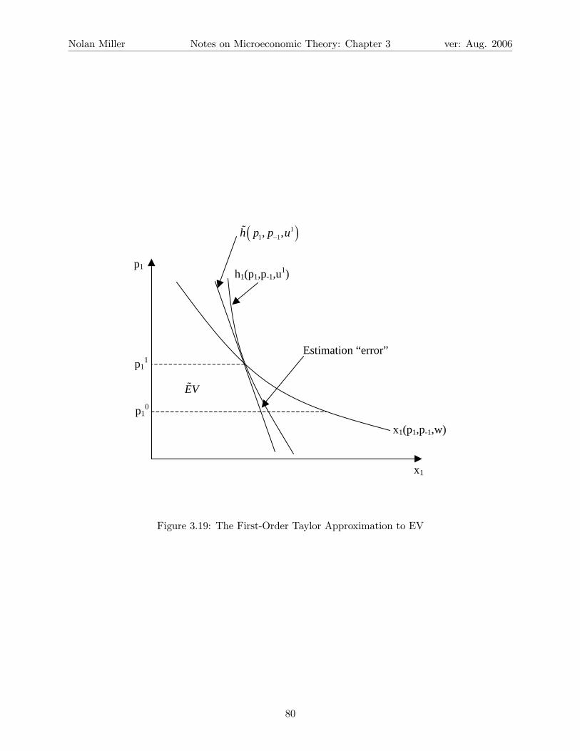
Nolan Miller Notes on Microeconomic Theory: Chapter 3 ver: Aug. 2006
x1(p1,p-1,w)
p11
p10
h1(p1,p-1,u1)
( )11 1, ,h p p u−
EV
Estimation “error”
p1
x1
Figure 3.19: The First-Order Taylor Approximation to EV
80

Nolan Miller Notes on Microeconomic Theory: Chapter 3 ver: Aug. 2006
x1(p1,p-1,w)
p11
p10
h1(p1,p-1,u0) ( )01 1, ,h p p u−
CV
Estimation “error”
p1
x1
Figure 3.20: The First-Order Taylor Approximation to CV
utility level, h1¡p1, p−1, u0
¢. Because of this, we must use the original price as the “original point”
in the Taylor approximation. Thus, for the purposes of CV, estimated Hicksian demand is given
by:
h1¡s, p0−1, u
1¢ ∼= h1
¡p01, p
0−1, u
1¢+
∂h1 (p, v (p,w))
∂p1
¡s− p01
¢∼= x1
¡p01, p
0−1, w
¢+
̶x1
¡p01, p
0−1, w
¢∂p1
+∂x1
¡p01, p
0−1, w
¢∂w
x1¡p01, p
0−1, w
¢!¡s− p01
¢.
The diagram for the Taylor approximation to CV corresponding to Figure 3.19 therefore looks like
Figure 3.20:
Welfare Evaluation: An Example
Data: x01 = 100, p01 = 10,
∂x∂p = −4,
∂x∂w = 0.02. Note: there is no information on w.
Suppose the price of good 1 increases to p0 = 12.5. How much should a public assistance
program aimed at maintaining a certain standard of living be increased to offset this price increase?
To answer this question, we are looking for the CV of the price change. To compute this, we
need to approximate the Hicksian demand curve for the original utility level, h1¡p1, p−1, u0
¢.
81

Nolan Miller Notes on Microeconomic Theory: Chapter 3 ver: Aug. 2006
12.5
10
100 95 90
Estimated Walrasian demand Estimated Hicksian demand
True Hicksian demand
Figure 3.21:
1. We know that h1¡10, p−1, u0
¢= x1 (10, p−1, w).
2. The slope of the h1¡p1, p−1, u0
¢can be approximated using the data and the Slutsky
equation.
∂h
∂p=
∂x
∂p+
∂x
∂wx
= −4 + 0.02 (100)
= −2
3. So, at price 12.5, Hicksian demand is given by
h = 100 +∂h
∂pdp
= 100 + (−2) 2.5 = 95
4. To compute CV, compute the area of a trapezoid (or the area of a rectangle plus a triangle):
|CV | = (2.5)µ95 + 100
2
¶= 243.75.
Since the price is increasing, we know that CV < 0, so CV = −243.75.
We could also estimate the change in Marshallian Consumer Surplus. This is just the area to
the left of the Walrasian demand curve between the two prices. Hence ∆CS = − (2.5)¡90+1002
¢=
−237.5. Hence if we were to use the Marshallian consumer surplus in this case, we would not
compensate the consumer enough for the price increase.
82

Nolan Miller Notes on Microeconomic Theory: Chapter 3 ver: Aug. 2006
Another thing we could do is figure that the harm done to the consumer is just the change in
price times the original consumption of this good, i.e., 2.5 (100) = 250. However, if we gave the
consumer 250 additional dollars, we would be overcompensating for the price increase.
3.4.9 Welfare Evaluation for an Arbitrary Price Change
The basic analysis of welfare change using CV and EV considers the case of a single price change.
However, what should we do if the policy change is not a single price change? For changes in
multiple prices, we can just compute the CV for each of the changes (i.e., changing prices one by
one and adding the CV (or EV) from each of the changes along a “path” from the original price to
the new price). If price and wealth change, we can add the change in wealth to the CV (or EV)
from the price changes (see below). But, what if the policy change involves something other than
prices and wealth, such a change in environmental quality, roads, etc. How do we value such a
change?
The answer is that, if we have good estimates of Walrasian demand, we can always represent
the change as a change in a budget set. After doing so, we can compute the CV is the usual way.
Part 1: Any arbitrary policy change can be thought of as a simultaneous change in
p and w.
To illustrate, suppose that we have a good estimate of consumers’ demand functions (i.e., we
fit a flexible functional form for demand using high-quality data). Let x (p,w) denote demand.
Suppose that initially prices and wealth are¡p0, w0
¢and the consumer chooses bundle x
¡p0, w0
¢.
Now, suppose that “something happens” that leads the consumer to choose bundle x0 instead of
x0. What is the CV (or EV) of this change?
The first step is to note that, if demand is quasiconcave, there is some price-wealth vector for
which x0 and x0 are optimal choices. You can find these price-wealth vectors, which we’ll call¡p0, w0
¢and (p0, w0), by solving the equations x0 =
¡p0, w0
¢and x0 = x (p0, w0). (In reality you
probably already know¡p0, w0
¢and have an observation of x0 or estimate of.) Remember, we have
a good estimate of x (p,w). Once we find (p0, w0), then we know that the change in the consumer’s
utility in going from x0 to x0is just v (p0, w0)− v
¡p0, w0
¢, and so the impact of the policy change
reduces to computing the EV or CV for this simultaneous change in p and w. Let v (p0, w0) = u0
and v¡p0, w0
¢= u0.
Part 2: Compute the EV or CV for a simultaneous change in p and w.
So, we’ve recast the policy change as a change from¡p0, w0
¢to (p0, w0), letting u0 and u0 denote
83

Nolan Miller Notes on Microeconomic Theory: Chapter 3 ver: Aug. 2006
the utility levels before and after the change. To compute EV , return to the definition of EV we
used before.
EV = e¡p0, u0
¢− e
¡p0, u0
¢Adding and subtracting e (p0, u0), we get:
EV =£e¡p0, u0
¢− e
¡p0, u0
¢¤+£e¡p0, u0
¢− e
¡p0, u0
¢¤.
But, note that e (p0, u0) = w0 and e¡p0, u0
¢= w0, so
EV =£e¡p0, u0
¢− e
¡p0, u0
¢¤+ w0 −w0, (*)
and note that£e¡p0, u0
¢− e (p0, u0)
¤is as in the definition of EV when only a price changes. So, if
only the price of good 1 changes, EV can be written as:
EV =
Z p01
p01
h1¡s, p−1, u
0¢ ds+ ¡w0 − w0¢,
and this can be estimated in the usual way from the estimated Walrasian demand curve.
If multiple prices change, we change them one by one and add up the integral from each change,
and then we add the change in wealth. That is, if prices change from¡p01, p
02, ..., p
0L
¢to (p01, p
02, ..., p
0L)
and wealth changes from w0 to w0, the EV is:
EV =
Z p01
p01
h1¡s, p02, ..., p
0L
¢ds+
Z p02
p02
h2¡p01, s, p
03, ..., p
0L
¢ds+...+
Z p0L
p0L
h2¡p01, p
02, ..., p
0L−1, s
¢ds+w0−w0.
If you replace each Hicksian demand with an estimate based on Marshallian demand and the Slutsky
equation, you can estimate this using only observables. It is tedious, but certainly possible.
This is a diagram that illustrates the whole thing. Suppose a policy change moves the con-
sumer’s consumption bundle from x0 to x0. To compute the EV, the first thing you do is find the
(p,w) for which x0 = x¡p0, w0
¢. This budget set is labeled B
¡p0, w0
¢. Then, you find the (p,w)
for which x0 is optimal, which we call (p0, w0). This budget set (red) is labeled B (p0, w0). Denote
the initial utility level u0 and the final utility level u0, and note that neither the utility levels nor
the indifference curves (which are drawn in as dotted lines for illustration) are observed.
Next, we decompose the change from¡p0, w0
¢to (p0, w0) into two parts. Part 1 is a change in
wealth holding prices fixed at p0. Let y denote the point the consumer chooses at¡p0, w0
¢, and
let uy denote the utiltiy earned. This point and the associated budget set are in blue. Note that
moving from budget set B¡p0, w0
¢to budget set B
¡p0, w0
¢is just like losing w0−w0 dollars (since
prices don’t change this is, in fact, exactly what happens). This is where the¡w0 −w0
¢term comes
84
Nolan Miller Notes on Microeconomic Theory: Chapter 3 ver: Aug. 2006
from in expression (*) above. Distance w0−w0 is denoted on the left. (Note that in the diagram,
these distances are scaled by p2, since we are showing them on the x2-axis.)
Part 2 of the decomposition is the change in prices from p0 to p0 when wealth is w0. But, note
that this just the kind of EV we computed in the simple case. That is, prices change but wealth
remains constant. Let z denote the point that offers the same utility as x0 but is chosen at prices
p0. That is, z = x¡p0, w0 +EV
¡p0, p0.w0
¢¢. The budget line supporting z is denoted in green, and
the EV for the price change from p0 to p0 at wealth w0 is just the distance that the budget shifts up
from blue B¡p0, w0
¢to green B
¡p0, w0 +EV
¡p0, p0.w0
¢¢denoted EV
¡p0, p0, w0
¢on the left. Since
EV¡p0, p0, w0
¢= e
¡p0, u0
¢− e
¡p0, uy
¢= e
¡p0, u0
¢−w0
= e¡p0, u0
¢− e
¡p0, u0
¢,
this is just like the EV’s we computed when only prices changed. This is where the£e¡p0, u0
¢− e (p0, u0)
¤comes from in expression (*) above.
The total EV is the sum of these two parts. The distance is denoted Total EV in the diagram.
Note that since the consumer ends up worse off overall, the total EV should be negative.
You could also do something similar for CV.
CV = e¡p0, u0
¢− e
¡p0, u0
¢=
£e¡p0, u0
¢− e
¡p0, u0
¢¤+he¡p0, u0
¢− e
³p0, u0´i
= w0 − w0 +he¡p0, u0
¢− e
³p0, u0´i,
and note that once again£e¡p0, u0
¢− e
¡p0, u0
¢¤is as in our original definition of CV . So, this
term can be rewritten in terms of integrals of Hicksian demand curves at utility level u0.
85

Nolan Miller Notes on Microeconomic Theory: Chapter 3 ver: Aug. 2006
x2
x0
x'
y
z
B(p0,w0)
B(p',w')
B(p0,w')
B(p',w'+EV(p0,p',w'))
w'-w0
EV(p0,p',w')
Total EV
u0
u'
uy
Figure 3.22:
86
Chapter 4
Topics in Consumer Theory
4.1 Homothetic and Quasilinear Utility Functions
One of the chief activities of economics is to try to recover a consumer’s preferences over all bundles
from observations of preferences over a few bundles. If you could ask the consumer an infinite
number of times, “Do you prefer x to y?”, using a large number of different bundles, you could do
a pretty good job of figuring out the consumer’s indifference sets, which reveals her preferences.
However, the problem with this is that it is impossible to ask the question an infinite number of
times.1 In doing economics, this problem manifests itself in the fact that you often only have a
limited number of data points describing consumer behavior.
One way that we could help make the data we have go farther would be if observations we made
about one particular indifference curve could help us understand all indifference curves. There are
a couple of different restrictions we can impose on preferences that allow us to do this.
The first restriction is called homotheticity. A preference relation is said to be homothetic if
the slope of indifference curves remains constant along any ray from the origin. Figure 4.1 depicts
such indifference curves.
If preferences take this form, then knowing the shape of one indifference curve tells you the
shape of all indifference curves, since they are “radial blowups” of each other. Formally, we say a
preference relation is homothetic if for any two bundles x and y such that x ∼ y, then αx ∼ αy
for any α > 0.
We can extend the definition of homothetic preferences to utility functions. A continuous
1 In fact, to completely determine the indifference sets you would have to ask an uncountably infinite number of
questions, which is even harder.
87

Nolan Miller Notes on Microeconomic Theory: Chapter 4 ver: Aug. 2006
x2
x1
Figure 4.1: Homothetic Preferences
preference relation º is homothetic if and only if it can be represented by a utility function that
is homogeneous of degree one. In other words, homothetic preferences can be represented by a
function u () that such that u (αx) = αu (x) for all x and α > 0. Note that the definition does
not say that every utility function that represents the preferences must be homogeneous of degree
one — only that there must be at least one utility function that represents those preferences and is
homogeneous of degree one.
EXAMPLE: Cobb-Douglas Utility: A famous example of a homothetic utility function is
the Cobb-Douglas utility function (here in two dimensions):
u (x1, x2) = xa1x1−a2 : a > 0.
The demand functions for this utility function are given by:
x1 (p,w) =aw
p1
x2 (p,w) =(1− a)w
p2.
Notice that the ratio of x1 to x2 does not depend on w. This implies that Engle curves (wealth
expansion paths) are straight lines (see MWG pp. 24-25). The indirect utility function is given
by:
v (p,w) =
µaw
p1
¶aµ(1− a)w
p2
¶1−a= w
µa
p1
¶aµ1− a
p2
¶1−a.
Another restriction on preferences that can allow us to draw inferences about all indifference
curves from a single curve is called quasilinearity. A preference relation is quasilinear if there is
one commodity, called the numeraire, which shifts the indifference curves outward as consumption
88
Nolan Miller Notes on Microeconomic Theory: Chapter 4 ver: Aug. 2006
of it increases, without changing their slope. Indifference curves for quasilinear preferences are
illustrated in Figure 3.B.6 of MWG.
Again, we can extend this definition to utility functions. A continuous preference relation
is quasilinear in commodity 1 if there is a utility function that represents it in the form u (x) =
x1 + v (x2, ..., xL).
EXAMPLE: Quasilinear utility functions take the form u (x) = x1 + v (x2, ..., xL). Since
we typically want utility to be quasiconcave, the function v () is usually a concave function such as
log x or√x. So, consider:
u (x) = x1 +√x2.
The demand functions associated with this utility function are found by solving:
maxx1 + x0.52
s.t. : p · x ≤ w
or, since x1 = −x2 p2p1 +wp1,
max−x2p2p1+
w
p1+ x0.52 .
The associated demand curves are
x1 (p,w) = −14
p1p2+
w
p1
x2 (p,w) =
µp12p2
¶2and indirect utility function:
v (p,w) =1
4
p1p2+
w
p1.
Isoquants of this utility function are drawn in Figure 4.2.
4.2 Aggregation
Our previous work has been concerned with developing the testable implications of the theory of
the consumer behavior on the individual level. However, in any particular market there are large
numbers of consumers. In addition, often in empirical work it will be difficult or impossible to
collect data on the individual level. All that can be observed are aggregates: aggregate consumption
of the various commodities and a measure of aggregate wealth (such as GNP). This raises the
89

Nolan Miller Notes on Microeconomic Theory: Chapter 4 ver: Aug. 2006
2 4 6 8 10x2
2
4
6
8
10
12
14
x1
Figure 4.2: Quasilinear Preferences
natural question of whether or not the implications of individual demand theory also apply to
aggregate demand.
To make things a little more concrete, suppose there are N consumers numbered 1 through N ,
and the nth consumer’s demand for good i is given by xni (p,wn), where wn is consumer n’s initial
wealth. In this case, total demand for good i can be written as:
Di
¡p,w1, ..., wN
¢=
NXn=1
xni (p,wn) .
However, notice that Di () gives total demand for good i as a function of prices and the wealth levels
of the n consumers. As I said earlier, often we will not have access to information about individuals,
only aggregates. Thus we may ask the question of when there exists a functionDi (p,w) , where w =PNn=1w
n is aggregate wealth, that represents the same behavior as Di
¡p,w1, ..., wN
¢. A second
question is when, given that there exists an aggregate demand function Di (p,w), the behavior
it characterizes is rational. We ask this question in two ways: First, when will the behavior
resulting from Di (p,w) satisfy WARP? Second, when will it be as if Di (p,w) were generated by a
“representative consumer” who is herself maximizing preferences? Finally, we will ask if there is a
representative consumer, in what sense is the well-being of the representative consumer a measure
of the well-being of society?
4.2.1 The Gorman Form
The major theme that runs through our discussion in this section is that in order for demand to
aggregate, each individual’s utility function must have an indirect utility function of the Gorman
90

Nolan Miller Notes on Microeconomic Theory: Chapter 4 ver: Aug. 2006
Form. So, let me take a moment to introduce the terminology before we need it. An indirect
utility function for consumer n, vn (p,w), is said to be of the Gorman Form if it can be written
in terms of functions an (p), which may depend on the specific consumer, and b (p), which does not
depend on the specific consumer:
vn (p,w) = an (p) + b (p)wn.
That is, an indirect utility function of the Gorman form can be separated into a term that depends
on prices and the consumer’s identity but not on her wealth, and a term that depends on a function
of prices that is common to all consumers that is multiplied by that consumer’s wealth.
The special nature of indirect utility functions of the Gorman Form is made apparent by applying
Roy’s identity:
xni (p,wn) = −
∂vn
∂pi∂vn
∂wn
= −ani (p) +
∂b(p)∂pi
wn
b (p). (4.1)
From now on, we will let bi (p) =∂b(p)∂pi
. Now consider the derivative of a particular consumer’s
demand for commodity i :∂xni (p,w
n)∂w = bi(p)
b(p) . This implies that wealth-expansion paths are given
by:∂xni (p,w
n)∂wn
∂xnj (p,wn)
∂wn
=bi (p)
bj (p).
Two important properties follow from these derivatives. First, for a fixed price, p, ∂xni (p,wn)
∂w does
not depend on wealth. Thus, as wealth increases, each consumer increases her consumption of the
goods at a linear rate. The result is that each consumer’s wealth-expansion paths are straight lines.
Second, ∂xni (p,w
n)∂w is the same for all consumers, since bi(p)
b(p) does not depend on n. This implies that
the wealth-expansion paths for different consumers are parallel (see MWG Figure 4.B.1).
Next, let’s aggregate the demand functions of consumers with Gorman form indirect utility
functions. Sum the individual demand functions from (4.1) across all n to get aggregate demand:
Di
¡p,w1, ..., wn
¢=
Xn
−ani (p)− bi (p)wn
b (p)=Xn
−ani (p)b (p)
− bi (p)
b (p)
Xwn
=Xn
−ani (p)b (p)
− bi (p)
b (p)wtotal.
Thus if all consumers have utility functions of the Gorman form, demand can be written solely as
a function of prices and total wealth. In fact, this is a necessary and sufficient condition: Demand
can be written as a function of prices and total wealth if and only if all consumers have indirect
utility functions of the Gorman form (see MWG Proposition 4.B.1).
91
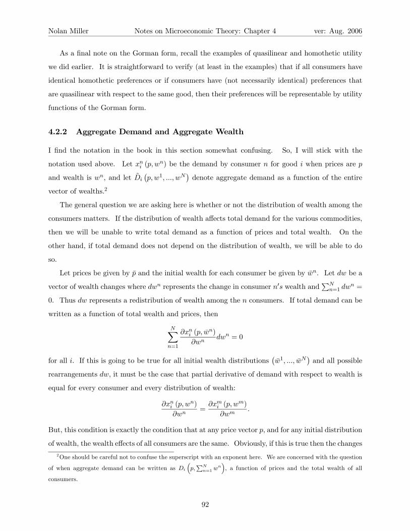
Nolan Miller Notes on Microeconomic Theory: Chapter 4 ver: Aug. 2006
As a final note on the Gorman form, recall the examples of quasilinear and homothetic utility
we did earlier. It is straightforward to verify (at least in the examples) that if all consumers have
identical homothetic preferences or if consumers have (not necessarily identical) preferences that
are quasilinear with respect to the same good, then their preferences will be representable by utility
functions of the Gorman form.
4.2.2 Aggregate Demand and Aggregate Wealth
I find the notation in the book in this section somewhat confusing. So, I will stick with the
notation used above. Let xni (p,wn) be the demand by consumer n for good i when prices are p
and wealth is wn, and let Di
¡p,w1, ..., wN
¢denote aggregate demand as a function of the entire
vector of wealths.2
The general question we are asking here is whether or not the distribution of wealth among the
consumers matters. If the distribution of wealth affects total demand for the various commodities,
then we will be unable to write total demand as a function of prices and total wealth. On the
other hand, if total demand does not depend on the distribution of wealth, we will be able to do
so.
Let prices be given by p and the initial wealth for each consumer be given by wn. Let dw be a
vector of wealth changes where dwn represents the change in consumer n0s wealth andPN
n=1 dwn =
0. Thus dw represents a redistribution of wealth among the n consumers. If total demand can be
written as a function of total wealth and prices, then
NXn=1
∂xni (p, wn)
∂wndwn = 0
for all i. If this is going to be true for all initial wealth distributions¡w1, ..., wN
¢and all possible
rearrangements dw, it must be the case that partial derivative of demand with respect to wealth is
equal for every consumer and every distribution of wealth:
∂xni (p,wn)
∂wn=
∂xmi (p,wm)
∂wm.
But, this condition is exactly the condition that at any price vector p, and for any initial distribution
of wealth, the wealth effects of all consumers are the same. Obviously, if this is true then the changes
2One should be careful not to confuse the superscript with an exponent here. We are concerned with the question
of when aggregate demand can be written as Di p, Nn=1 w
n , a function of prices and the total wealth of all
consumers.
92
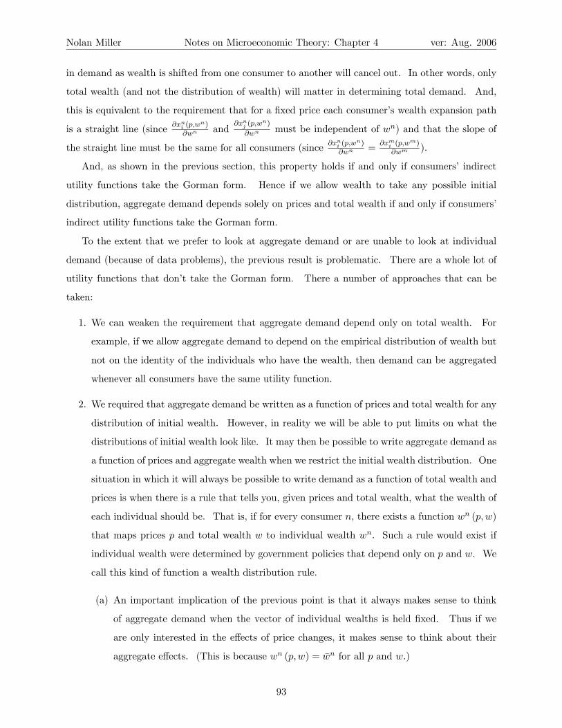
Nolan Miller Notes on Microeconomic Theory: Chapter 4 ver: Aug. 2006
in demand as wealth is shifted from one consumer to another will cancel out. In other words, only
total wealth (and not the distribution of wealth) will matter in determining total demand. And,
this is equivalent to the requirement that for a fixed price each consumer’s wealth expansion path
is a straight line (since ∂xni (p,wn)
∂wn and∂xnj (p,w
n)
∂wn must be independent of wn) and that the slope of
the straight line must be the same for all consumers (since ∂xni (p,wn)
∂wn =∂xmi (p,w
m)∂wm ).
And, as shown in the previous section, this property holds if and only if consumers’ indirect
utility functions take the Gorman form. Hence if we allow wealth to take any possible initial
distribution, aggregate demand depends solely on prices and total wealth if and only if consumers’
indirect utility functions take the Gorman form.
To the extent that we prefer to look at aggregate demand or are unable to look at individual
demand (because of data problems), the previous result is problematic. There are a whole lot of
utility functions that don’t take the Gorman form. There a number of approaches that can be
taken:
1. We can weaken the requirement that aggregate demand depend only on total wealth. For
example, if we allow aggregate demand to depend on the empirical distribution of wealth but
not on the identity of the individuals who have the wealth, then demand can be aggregated
whenever all consumers have the same utility function.
2. We required that aggregate demand be written as a function of prices and total wealth for any
distribution of initial wealth. However, in reality we will be able to put limits on what the
distributions of initial wealth look like. It may then be possible to write aggregate demand as
a function of prices and aggregate wealth when we restrict the initial wealth distribution. One
situation in which it will always be possible to write demand as a function of total wealth and
prices is when there is a rule that tells you, given prices and total wealth, what the wealth of
each individual should be. That is, if for every consumer n, there exists a function wn (p,w)
that maps prices p and total wealth w to individual wealth wn. Such a rule would exist if
individual wealth were determined by government policies that depend only on p and w. We
call this kind of function a wealth distribution rule.
(a) An important implication of the previous point is that it always makes sense to think
of aggregate demand when the vector of individual wealths is held fixed. Thus if we
are only interested in the effects of price changes, it makes sense to think about their
aggregate effects. (This is because wn (p,w) = wn for all p and w.)
93

Nolan Miller Notes on Microeconomic Theory: Chapter 4 ver: Aug. 2006
4.2.3 Does individual WARP imply aggregate WARP?
The next aggregation question we consider is whether the fact that individuals make consistent
choices implies that aggregate choices will be consistent as well. In terms of our discussion in
Chapter 2, this involves the question of whether, when the Walrasian demand functions of the N
consumers satisfy WARP, the resulting aggregate demand function will satisfy WARP as well. The
answer to this question is, “Not necessarily.”
To make things concrete, assume that there is a wealth distribution rule, so that it makes sense
to talk about aggregate demand as D (p,w) = (D1 (p,w) , ...,DL (p,w)). In fact, to keep things
simple, assume that the wealth distribution rule is that wn (p,w) = anw. Thus consumer n is
assigned a fraction an of total wealth. Thus
D (p,w) =Xn
xn (p,wn) .
The aggregate demand function satisfies WARP if, for any two combinations of prices and
aggregate wealth, (p,w) and (p0, w0), if p·D (p0, w0) ≤ w andD (p,w) 6= D (p0, w0), then p0·D (p,w) >
w0. This is the same definition of WARP as before.
The reason why individual WARP is not sufficient for aggregate WARP has to do with the
Compensated Law of Demand (CLD). Recall that an individual’s behavior satisfies WARP if and
only if the CLD holds for all possible compensated price changes. The same is true for aggregate
WARP. The aggregate will satisfy WARP if and only if the CLD holds in the aggregate for all
possible compensated price changes. The problem is that just because a price change is compen-
sated in the aggregate, it does not mean that the price change is compensated for each individual.
Because of this, it does not necessarily follow from the fact that each individual’s behavior satisfies
the CLD that the aggregate will as well, since compensated changes in the aggregate need not
imply compensated changes individually. See Example 4.C.1 and Figure 4.C.1 in MWG.
To make this a little more concrete without going into the details of the argument, think about
how you would prove this statement: “If individuals satisfy WARP then the aggregate does as
well.” The steps would be:
1. Consider a compensated change in aggregate wealth.
2. This can be written as a sum of compensated changes in individual wealths.3
3Of course, this step is not true!
94

Nolan Miller Notes on Microeconomic Theory: Chapter 4 ver: Aug. 2006
3. Individuals satisfy WARP if and only if they satisfy the CLD.
4. So, each individual change satisfies the CLD.
5. Adding over individual changes, the aggregate satisfies the CLD as well.
This proof is clearly flawed since step 2 is not valid. As shown above, it is not possible to
write every price change that is compensated in the aggregate in terms of price changes that are
compensated individual-by-individual. So, it turns out that satisfying WARP and therefore the
CLD is not sufficient for aggregate decisions to satisfy WARP. However, if we impose stronger
conditions on individual behavior, we can find a property that aggregates. That property is the
Uncompensated Law of Demand (ULD). The ULD is similar to the CLD, but it involves
uncompensated changes. Thus a demand function x (p,w) satisfies the ULD if for any price change
p→ p0 the following holds: ¡p0 − p
¢ ¡x¡p0, w
¢− x (p,w)
¢≤ 0.
Note the following:
1. If a consumer’s demand satisfies the ULD, then it satisfies the CLD as well.
2. Unlike the CLD, the ULD aggregates. Thus if each consumer’s demand satisfies the ULD,
the aggregate demand function will as well.
Hence even though satisfaction of the CLD individually is not sufficient for the CLD in the
aggregate, the ULD individually is sufficient for the ULD in the aggregate. So, the ULD individually
implies WARP in the aggregate.
If we want to know which types of utility functions imply aggregate demand functions that
satisfy WARP, we need to find those that satisfy the ULD. It turns out that homothetic preferences
satisfy the ULD. Thus if each consumer has homothetic preferences, the implied aggregate demand
will satisfy WARP.
In general, there is a calculus test to determine if a utility function satisfies the ULD property.
It is given in MWG, and my advice is that if you ever need to know about such things, you look it
up at that time. Basically, it has to do with making sure that wealth effects are not too strange
(recall the example of the Giffen good — where the wealth effect leads to an upward sloping demand
curve — the same sort of thing is a concern here).
95

Nolan Miller Notes on Microeconomic Theory: Chapter 4 ver: Aug. 2006
4.2.4 Representative Consumers
The final question is when can the aggregate demand curve be used to make welfare measurements?
In other words, when can we treat aggregate demand as if it is generated by a fictional “represen-
tative consumer,” and when will changes in the welfare of that consumer correspond to changes in
the welfare of society as a whole?
The first part of this question is, when is there a rational preference relation º such that
the aggregate demand function corresponds to the Walrasian demand function generated by these
preferences? If such a preference relation exists, we say that there is a positive representative
consumer.
The first necessary condition for the existence of a positive representative consumer is that it
makes sense to aggregate demand. Thus consumers must have indirect utility functions of the
Gorman form (or wealth must be assigned by a wealth-assignment rule). In addition, the demand
must correspond to that implied by the maximization of some rational preference relation. In
essence, we need the Slutsky matrix to be negative semi-definite as well.
An additional question is whether the preferences of the positive representative consumer cap-
ture the welfare of society as a whole. This is the question of whether the positive representative
consumer is normative as well. For example, suppose there is a social welfare function
W (u1, ..., uN ) that maps utility levels for the N consumers to real numbers and such that utility
vectors assigned higher numbers are better for the society than vectors assigned lower numbers.
Thus W () is like a utility function for the society. Now suppose that for any level of aggregate
wealth we assign wealth to the consumers in order to maximize W . That is, w1, ..., wN solves
maxw1,...,wN
W¡v1¡p,w1
¢, ..., vN
¡p,wN
¢¢s.t.
NXn=1
wn ≤ w.
Thus it corresponds to the situation where a benevolent dictator distributes wealth in the society in
order to maximize social welfare. This defines a wealth assignment rule, so we know that aggregate
demand can be represented as a function of p and total wealth w.
In the case where wealth is assigned as above, not only can demand be written as D (p,w), but
also these demand functions are consistent with the existence of a positive representative consumer.
Further, if the aggregate demand functions are generated by solving the previous program, they
have welfare significance and can be used to make welfare judgments (using the techniques from
96
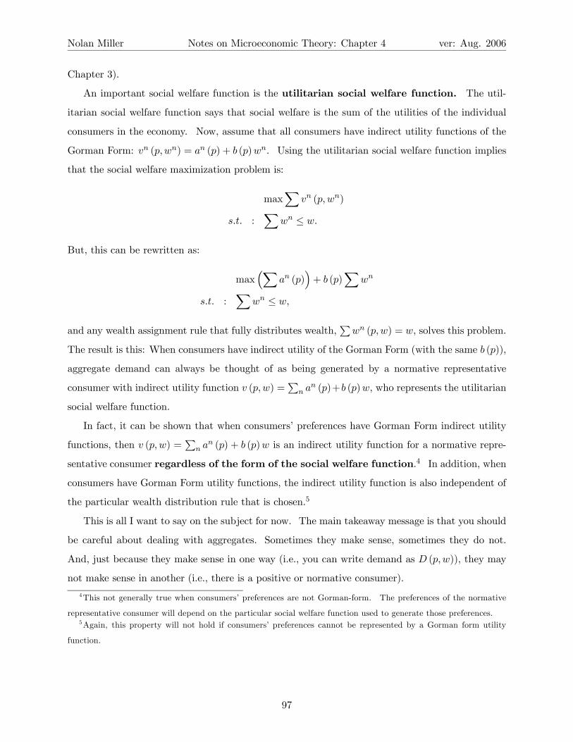
Nolan Miller Notes on Microeconomic Theory: Chapter 4 ver: Aug. 2006
Chapter 3).
An important social welfare function is the utilitarian social welfare function. The util-
itarian social welfare function says that social welfare is the sum of the utilities of the individual
consumers in the economy. Now, assume that all consumers have indirect utility functions of the
Gorman Form: vn (p,wn) = an (p) + b (p)wn. Using the utilitarian social welfare function implies
that the social welfare maximization problem is:
maxX
vn (p,wn)
s.t. :X
wn ≤ w.
But, this can be rewritten as:
max³X
an (p)´+ b (p)
Xwn
s.t. :X
wn ≤ w,
and any wealth assignment rule that fully distributes wealth,P
wn (p,w) = w, solves this problem.
The result is this: When consumers have indirect utility of the Gorman Form (with the same b (p)),
aggregate demand can always be thought of as being generated by a normative representative
consumer with indirect utility function v (p,w) =P
n an (p)+b (p)w, who represents the utilitarian
social welfare function.
In fact, it can be shown that when consumers’ preferences have Gorman Form indirect utility
functions, then v (p,w) =P
n an (p) + b (p)w is an indirect utility function for a normative repre-
sentative consumer regardless of the form of the social welfare function.4 In addition, when
consumers have Gorman Form utility functions, the indirect utility function is also independent of
the particular wealth distribution rule that is chosen.5
This is all I want to say on the subject for now. The main takeaway message is that you should
be careful about dealing with aggregates. Sometimes they make sense, sometimes they do not.
And, just because they make sense in one way (i.e., you can write demand as D (p,w)), they may
not make sense in another (i.e., there is a positive or normative consumer).
4This not generally true when consumers’ preferences are not Gorman-form. The preferences of the normative
representative consumer will depend on the particular social welfare function used to generate those preferences.5Again, this property will not hold if consumers’ preferences cannot be represented by a Gorman form utility
function.
97

Nolan Miller Notes on Microeconomic Theory: Chapter 4 ver: Aug. 2006
4.3 The Composite Commodity Theorem
There are many commodities in the world, but usually economists will only be interested in a few
of them at any particular time. For example, if we are interested in studying the wheat market,
we may divide the set of commodities into “wheat” and “everything else.” In a more realistic
setting, an empirical economist may be interested in the demand for broad categories of goods such
as “food,” “clothing,” “shelter,” and “everything else.” In this section, we consider the question
of when it is valid to group commodities in this way.6
To make things simple, consider a three-commodity model. Commodity 1 is the commodity we
are interested in, and commodities 2 and 3 are “everything else.” Denote the initial prices of goods
2 and 3 by p02 and p03, and suppose that if prices change, the relative price of goods 2 and 3 remain
fixed. That is, the price of goods 2 and 3 can always be written as p2 = tp02 and p3 = tp03, for
t ≥ 0. For example, if good 2 and good 3 are apples and oranges, this says that whenever the price
of apples rises, the price of oranges also rises by the same proportion. Clearly, this assumption
will be reasonable in some cases and unreasonable in others, but for the moment will will assume
that this is the case.
The consumer’s expenditure minimization problem can be written as:
minx≥0
p1x1 + tp02x2 + tp03x3
s.t. : u (x) ≥ u.
Solving this problem yields Hicksian demand functions h¡p1, tp
02, tp
03, u¢and expenditure function
e¡p1, tp
02, tp
03, u¢.
Now, suppose that we are interested only in knowing how consumption of good 1 depends on t.
In this case, we can make the following change of variables. Let y = p02x2+ p03x3. Thus y is equal
to expenditure on goods 2 and 3, and t then corresponds to the “price” of this expenditure. As t
increases, y becomes more expensive. Applying this change of variable to the h () and e () yields
the new functions:
h∗ (p1, t, u) ≡ h¡p1, tp
02, tp
03, u¢
e∗ (p1, t, u) ≡ e¡p1, tp
02, tp
03, u¢.
6References: Silberberg, Section 11.3; Deaton and Muellbauer Economics and Consumer Behavior, pp. 120-122;
Jehle and Reny, p. 266.
98

Nolan Miller Notes on Microeconomic Theory: Chapter 4 ver: Aug. 2006
It remains to be shown that h∗ () and e∗ () satisfy the properties of well-defined compensated
demand and expenditure functions (see Section 3.4). For e∗ (p1, t, u), these include:
1. Homogeneity of degree 1 in p
2. Concavity in (p1, t) (i.e. the Slutsky matrix is negative semi-definite)
3. ∂e∗
∂t = y (and the other associated derivative properties)
In fact, these relationships can be demonstrated. Hence we have the composite commodity
theorem:
Theorem 8 When the prices of a group of commodities move in parallel, then the total expenditure
on the corresponding group of commodities can be treated as a single good.
The composite commodity theorem has a number of important applications. First, the com-
posite commodity theorem can be used to justify the two-commodity approach that is frequently
used in economic models. If we are interested in the effect of a change in the price of wheat on
the wheat market, assuming that all other prices remain fixed, the composite commodity theorem
justifies treating the world as consisting of wheat and the composite commodity “everything else.”
A second application of the composite commodity theorem is to models of consumption over
time, which we will cover later (see Section 4.6 of these notes). Since the prices of goods in future
periods will tend to move together, application of the composite commodity theorem allows us
to analyze consumption over time in terms of the composite commodities “consumption today,”
“consumption tomorrow,” etc.
4.4 So Were They Just Lying to MeWhen I Studied Intermediate
Micro?
Recall from your intermediate microeconomics course that you probably did welfare evaluation by
looking at changes in Marshallian consumer surplus, the area to the left of the aggregate demand
curve. But, I’ve told you that: a) consumer surplus is not a good measure of the welfare of an
individual consumer; b) even if it were, it usually doesn’t make sense to think of aggregate demand
as depending only on aggregate wealth (which it does in the standard intermediate micro model);
and c) even if it did, looking at the equivalent variation (which is better than looking at the change
99

Nolan Miller Notes on Microeconomic Theory: Chapter 4 ver: Aug. 2006
in consumer surplus) for the aggregate demand curve may not have welfare significance. So, at
this point, most students are a little concerned that everything they learned in intermediate micro
was wrong. The point of this interlude is to argue that this is not true. Although many of the
assumptions made in order to simplify the presentation in intermediate micro are not explicitly
stated, they can be explicitly stated and are actually pretty reasonable.
To begin, note that the point of intermediate micro is usually to understand the impact of
changes on one or a few markets. For example, think about the change in the price of apples on
the demand for bananas. It is widely believed that since expenditure on a particular commodity
(like apples or bananas) is usually only a small portion of a consumer’s budget, the income effects
of changes in the prices of these commodities are likely to be small. In addition, since we are
looking at only a few price changes and either holding all other prices constant or varying them in
tandem, we can apply the composite commodity theorem and think of the consumer’s problem as
depending on the commodity in question and the composite commodity “everything else.” Thus
the consumer can be thought of as having preferences over apples, bananas, and everything else.
Now, since the income effects for apples and bananas are likely to be small, a reasonable way to
represent the consumer’s preferences is as being quasilinear in “everything else.” That is, utility
looks like:
u (a, b, e) = f (a, b) + e
where a = apples, b = bananas, and e = everything else. Once we agree that this is a reasonable
representation of preferences for our purposes, we can point out the following:
1. Since there are no wealth effects for apples or bananas, the Walrasian and Hicksian demand
curves coincide, and the change in Marshallian consumer surplus is the same as EV. Hence
∆CS is a perfectly fine measure of changes in welfare.
2. If all individual consumers in the market have utility functions that are quasilinear in every-
thing else, then it makes sense to write demand as a function of aggregate wealth, since
quasilinear preferences can be represented by indirect utility functions of the Gorman form.
3. Since all individuals have Gorman form indirect utility functions, then aggregate demand
can always be thought of as corresponding to a representative consumer for a social welfare
function that is utilitarian. Thus ∆CS computed using the aggregate demand curve has
welfare significance.
100

Nolan Miller Notes on Microeconomic Theory: Chapter 4 ver: Aug. 2006
Thus, by application of the composite commodity theorem and quasilinear preferences, we can
save the intermediate micro approach. Of course, our ability to do this depends on looking at only
a few markets at a time. If we are interested in evaluating changes in many or all prices, this may
not be reasonable. As you will see later, this merely explains why partial equilibrium is a topic for
intermediate micro and general equilibrium is a topic for advanced micro.
4.5 Consumption With Endowments
Until now we have been concerned with consumers who are endowed with initial wealth w. However,
an alternative approach would be to think of consumers as being endowed with both wealth w
and a vector of commodities a = (a1, ..., aL) , where ai gives the consumer’s initial endowment of
commodity i.7 In this case, the consumer’s UMP can be written as:
maxx
u (x)
s.t. : p · x ≤ p · a+ w
The value of the consumer’s initial assets is given by the sum of her wealth and the value of
her endowment, p · a. Thus the mathematical approach is equivalent to the situation where the
consumer first sells her endowment and then buys the best commodity bundle she can afford at
those prices.
The first-order conditions for this problem are found in the usual way. The Lagrangian is given
by:
L = u (x) + λ (p · a+ w − p · x)
implying optimality conditions:
ui − λpi = 0 : i = 1, ..., L.
p · x− p · a− w ≤ 0.
Denote the solution to this problem as
x (p,w, a)
where w is non-endowment wealth and a is the consumer’s initial endowment.7Reference: Silberberg (3rd edition), pp. 299-304.
101

Nolan Miller Notes on Microeconomic Theory: Chapter 4 ver: Aug. 2006
We can also solve a version of the expenditure minimization problem in this context. Consider
the problem:
minx
p · x− p · a
s.t. : u (x) ≥ u.
The objective function in this model is non-endowment wealth. Thus it plays the role of w in the
UMP, and the question asked by this problem can be stated as: How much non-endowment wealth
is needed to achieve utility level u when prices are p and the consumer is endowed with a?
The endowment a drops out of the Lagrangian when you differentiate with respect to xi. Hence
the non-endowment expenditure minimizing bundle (NEEMB) is not a function of a. We’ll continue
to denote it as h (p, u). However, while the NEEMB does not depend on a, the non-endowment
expenditure function does. Let
e∗ (p, u, a) ≡ p · (h (p, u)− a) .
Again, e∗ (p, u, a) represents the non-endowment wealth necessary to achieve utility level u as a
function of p and endowment a. By the envelope theorem (or the derivation for ∂e∂pi
= hi (p, u) we
did in Section 3.4.3) it follows that
∂e∗
∂pi≡ hi (p, u)− ai.
Thus the sign of ∂e∗
∂pidepends on whether hi (p, u) > ai or hi (p, u) < ai. If hi (p, u) > ai the
consumer is a net purchaser of good i, consuming more of it than her initial endowment. If this is
the case, then an increase in pi increases the cost of purchasing the good i from the market, and
this increases total expenditure at a rate of hi (p, u)−ai. On the other hand, if hi (p, u) < ai, then
the consumer is a net seller of good i, consuming less of it than her initial endowment. In this case,
increasing pi increases the revenue the consumer earns by selling the good to the market. The
result is that the non-endowment wealth the consumer needs to achieve utility level u decreases at
a rate of |hi (p, u)− ai|.
Now, let’s rederive the Slutsky equation in this environment. The following identity relates
h () and x ():
hi (p, u) ≡ xi (p, e∗ (p, u, a) , a) .
102
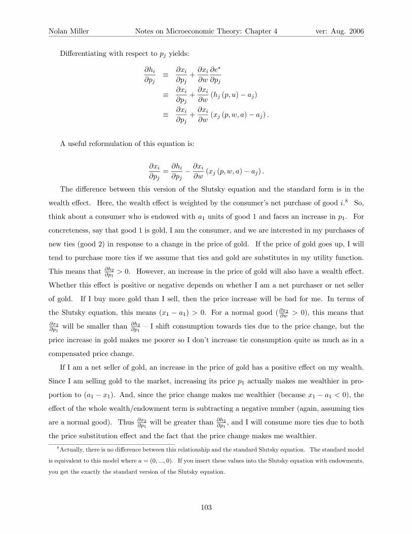
Nolan Miller Notes on Microeconomic Theory: Chapter 4 ver: Aug. 2006
Differentiating with respect to pj yields:
∂hi∂pj
≡ ∂xi∂pj
+∂xi∂w
∂e∗
∂pj
≡ ∂xi∂pj
+∂xi∂w
(hj (p, u)− aj)
≡ ∂xi∂pj
+∂xi∂w
(xj (p,w, a)− aj) .
A useful reformulation of this equation is:
∂xi∂pj
=∂hi∂pj− ∂xi
∂w(xj (p,w, a)− aj) .
The difference between this version of the Slutsky equation and the standard form is in the
wealth effect. Here, the wealth effect is weighted by the consumer’s net purchase of good i.8 So,
think about a consumer who is endowed with a1 units of good 1 and faces an increase in p1. For
concreteness, say that good 1 is gold, I am the consumer, and we are interested in my purchases of
new ties (good 2) in response to a change in the price of gold. If the price of gold goes up, I will
tend to purchase more ties if we assume that ties and gold are substitutes in my utility function.
This means that ∂h2∂p1
> 0. However, an increase in the price of gold will also have a wealth effect.
Whether this effect is positive or negative depends on whether I am a net purchaser or net seller
of gold. If I buy more gold than I sell, then the price increase will be bad for me. In terms of
the Slutsky equation, this means (x1 − a1) > 0. For a normal good (∂x2∂w > 0), this means that
∂x2∂p1
will be smaller than ∂h2∂p1
— I shift consumption towards ties due to the price change, but the
price increase in gold makes me poorer so I don’t increase tie consumption quite as much as in a
compensated price change.
If I am a net seller of gold, an increase in the price of gold has a positive effect on my wealth.
Since I am selling gold to the market, increasing its price p1 actually makes me wealthier in pro-
portion to (a1 − x1). And, since the price change makes me wealthier (because x1 − a1 < 0), the
effect of the whole wealth/endowment term is subtracting a negative number (again, assuming ties
are a normal good). Thus ∂x2∂p1
will be greater than ∂h2∂p1, and I will consume more ties due to both
the price substitution effect and the fact that the price change makes me wealthier.
8Actually, there is no difference between this relationship and the standard Slutsky equation. The standard model
is equivalent to this model where a = (0, ..., 0). If you insert these values into the Slutsky equation with endowments,
you get the exactly the standard version of the Slutsky equation.
103

Nolan Miller Notes on Microeconomic Theory: Chapter 4 ver: Aug. 2006
w
Leisure (l) 24
Expenditure (y)
y = w + s(24 - l)
(y*, l*)
Figure 4.3: Labor-Leisure Choice
Thus the main difference between the standard model and the endowment model lies in this
adjustment to the Slutsky matrix: The wealth effect must be adjusted by whether a consumer
is a net purchaser or a net seller of the good in question. This has important applications in
general equilibrium theory (which we’ll return to much later), as well as applications in applied
consumption models. We turn to one such example here.
4.5.1 The Labor-Leisure Choice
As an application of the previous section, consider a consumer’s choice between labor and leisure.
We are interested in the consumer’s leisure decision, so we’ll apply the composite commodity theo-
rem and model the consumer as caring about leisure, l, and everything else, y. Let the consumer’s
utility function be
u (y, l) .
If the wage rate is s, w is non-endowment wealth, and the price of “everything else” is normalized
to 1, the consumer’s budget constraint is given by:
y ≤ s (24− l) + w.
The solution to this problem is given by the point of tangency between the utility function and the
budget set. This point is illustrated in the Figure 4.3.
Initially, the consumer is endowed with 24 hours of leisure per day. Since the consumer cannot
consume more than 24 hours of leisure per day, at the optimum the consumer must be a net seller
104
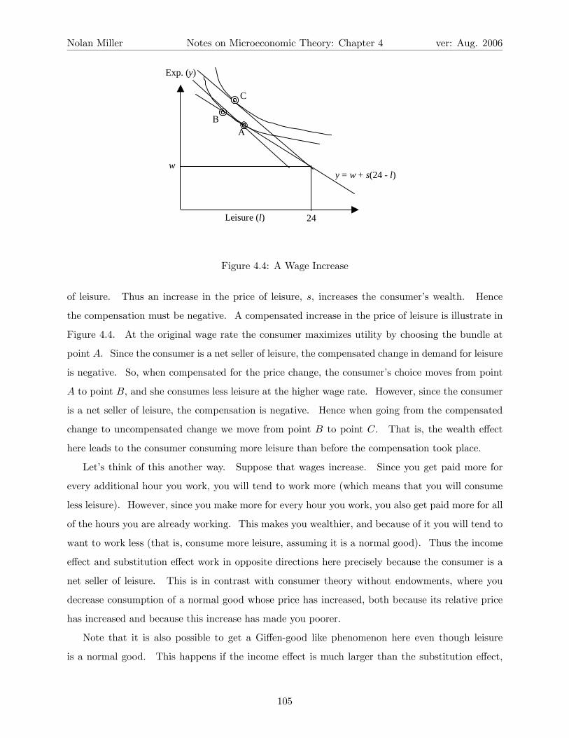
Nolan Miller Notes on Microeconomic Theory: Chapter 4 ver: Aug. 2006
w
Leisure (l) 24
Exp. (y)
y = w + s(24 - l)
A
C
B
Figure 4.4: A Wage Increase
of leisure. Thus an increase in the price of leisure, s, increases the consumer’s wealth. Hence
the compensation must be negative. A compensated increase in the price of leisure is illustrate in
Figure 4.4. At the original wage rate the consumer maximizes utility by choosing the bundle at
point A. Since the consumer is a net seller of leisure, the compensated change in demand for leisure
is negative. So, when compensated for the price change, the consumer’s choice moves from point
A to point B, and she consumes less leisure at the higher wage rate. However, since the consumer
is a net seller of leisure, the compensation is negative. Hence when going from the compensated
change to uncompensated change we move from point B to point C. That is, the wealth effect
here leads to the consumer consuming more leisure than before the compensation took place.
Let’s think of this another way. Suppose that wages increase. Since you get paid more for
every additional hour you work, you will tend to work more (which means that you will consume
less leisure). However, since you make more for every hour you work, you also get paid more for all
of the hours you are already working. This makes you wealthier, and because of it you will tend to
want to work less (that is, consume more leisure, assuming it is a normal good). Thus the income
effect and substitution effect work in opposite directions here precisely because the consumer is a
net seller of leisure. This is in contrast with consumer theory without endowments, where you
decrease consumption of a normal good whose price has increased, both because its relative price
has increased and because this increase has made you poorer.
Note that it is also possible to get a Giffen-good like phenomenon here even though leisure
is a normal good. This happens if the income effect is much larger than the substitution effect,
105

Nolan Miller Notes on Microeconomic Theory: Chapter 4 ver: Aug. 2006
w
Leisure (l) 24
Expenditure (y)
y = w + s(24 - l)
A
CB
Figure 4.5: Positive Labor Supply Elasticity
as in Figure 4.5, where the arrows depict the large income effect (point B to point C). As an
illustration, think of the situation in which a person earns minimum wage, let’s say $5 per hour, and
chooses to work 60 hours per week. That gives total wages of $300 per week. If the government
raises the minimum wage by $1 per hour, this increases the consumer’s total wages to $360, a 20%
increase. The consumer likely has two responses to this. Since the consumer gets paid more for
each additional hour of work, she may decide to work more hours (since she will be willing to give
up more leisure at the higher wage rate). However, since the $1 increase in wages has increased
total wage revenue by 20% already, this may make the consumer work less, since she is already
richer than before. In situations where the change in total wages is large relative to the wage rate
(i.e., the consumer is working a lot of hours), the latter effect may swamp the former.
There have been many studies of this labor-leisure tradeoff in the U.S. They are frequently
associated with worries over whether raising taxes on the wealthy will cause them to cut their labor
supply. My understanding of the evidence (through conversations with labor economists mostly)
is that labor supply elasticities are positive but small, similar to the depiction in Figure 4.5.9
4.5.2 Consumption with Endowments: A Simple Separation Theorem
The first half of the course deals with doing welfare evaluation correctly. The second half of the
course deals with markets and market interactions. One of the themes I will try to bring out is
9 In fact, labor supply elasticities tend to be pretty small for men, larger for women, but always positive (i.e. an
increase in wages - or a cut in income taxes - leads people to work more).
106

Nolan Miller Notes on Microeconomic Theory: Chapter 4 ver: Aug. 2006
the idea that when markets work well, people make good decisions. That is, they make decisions
that maximize economic value, and then they use markets to buy and sell commodities to arrive at
the consumption bundle they want. Remarkably, it turns out that when markets are perfect, this
approach also maximizes the consumer’s welfare. However, if markets do not function well, then
people may be forced to distort their decisions to make up for the fact that they cannot use markets
to modify their consumption bundle. For example, if markets are perfect and the price of bananas
is high and the price of coconuts is low, even a farmer who hates bananas and loves coconuts will
be best off by choosing to grow bananas. But, once the bananas are harvested he will sell them
and use the proceeds to purchase coconuts. In this way, he will be able to eat more coconuts
than if he grew them himself. If there are not good markets, then the farmer will be forced to eat
what he grows. In this case, he will be forced to grow coconuts, and he will end up with fewer
coconuts than he would have if the markets were better. In addition to the “micro” effects, there
can also be larger scale effects. If everyone makes suboptimal decisions because markets are not
well developed, then overall growth may be adversely impacted.
To illustrate, consider a consumer who must choose between endowment a = (a1, a2) and
endowment b = (b1, b2). (Assume non-endowment wealth is w = 0 for the sake of the diagrams.)
How should the consumer choose? If markets are perfect, the consumer should choose whichever
bundle has the higher market value. After all, if bundle a has higher market value than bundle
b, then the budget set for endowment a includes the budget set for endowment b, and therefore
the consumer must be strictly better off at a than b. Thus, a  b if and only if p · a > p · b.
Figure 1 illustrates. Note, however, that a critical assumption underlying this is that the price at
which you can buy a commodity is the same as the price at which you can sell it. This is often
not the case. In fact, it is the norm in markets for the “buy price” to be greater than the “sell
price,” and the extent to which the two differ is often interpreted as a sign of market development
or competitiveness.
Next, consider the case where the buy price of a good is greater than the sell price. Let pb1 and
pb2 denote the buy prices and ps1 and p
s2 denote the sell prices, and suppose p
b1 > ps1 and p
b2 > ps2. In
this case, the budget set will have a kink at the endowment point. Above the endowment point,
the slope of the budget line is −ps1pb2(since over this range the consumer is selling x1 and using the
money he makes to buy x2). Below the endowment point, the slope of the budget line is −pb1ps2, since
over this range the consumer is selling good 2 and using the profit to buy good 1. (See Figure 2.)
Since pb1 > ps1 and pb2 > ps2, the slope is steeper when the consumer buys 1 and sells 2 than when
107

Nolan Miller Notes on Microeconomic Theory: Chapter 4 ver: Aug. 2006
a
b
x1
x2
p1 x1 + p2 x2 = p1 a1 + p2 a2
p1 x1 + p2 x2 = p1 b1 + p2 b2
Figure 4.6:
he sells 1 and buys 2. (If you don’t believe me, plug in some numbers for pb1, ps1, p
b2, and ps2.)
Now, return to the question of whether the consumer should prefer endowment a or endowment
b. Now the answer to the question is: “it depends.” Consider Figure 3. In this case, whether the
consumer prefers a or b will depend on the nature of his preferences. If he has a strong preference
for good x1, he may choose endowment b. This is true even though the “market value” of a would
be larger if there were no bid-ask spread.
Thus, the inability to increase consumption of x1 through the market may lead the consumer
to make decisions that maximize short run utility but have negative long-run consequences. For
example, if x1 is a food crop and x2 is a non-food crop, then a represents focusing on the cash crop
while b represents focusing on the subsistence crop. If markets are good, the consumer should grow
the cash crop and use the market to purchase food. If markets are not good, then the consumer
will have to grow the food crop, passing on the opportunity to increase welfare by growing the cash
crop.
This is known as a “separation result” because it essentially says that if markets are perfect,
then the consumer’s production decision (which endowment to choose) and consumption decision
(what to consume) can be separated. The consumer maximizes welfare by making the production
108

Nolan Miller Notes on Microeconomic Theory: Chapter 4 ver: Aug. 2006
a
x1
x2 slope –(p1s/p2
b)
sell x1
buy x2
slope –(p1b/p2
s)
sell x2
buy x1
Figure 4.7:
a
x1
x2
b
Figure 4.8:
109

Nolan Miller Notes on Microeconomic Theory: Chapter 4 ver: Aug. 2006
decision that maximizes the value of the endowment and then maximizes utility given the resulting
budget set. We will see these kind of results in a wide variety of circumstances. Often, and
especially in a developing context, the real importance of these results is not when they work (since
markets are never perfect!), but when they don’t. In this case, separation results suggest that
improving markets can improve welfare. This is much more interesting and useful than the way
the result is usually stated.
4.6 Consumption Over Time
Up until now we have been considering a model of consumption that is static. Time does not enter
into our model at all. This model is very useful for modeling a consumer’s behavior at a particular
point in time. It is also useful for modeling the consumer’s behavior in two different situations.
This is what we called “comparative statics.” However, as the name suggests, even though the
consumer’s behavior in two different situations can be compared using the static model, we are
really just comparing two static situations: No attempt is made to model how the consumer’s
behavior evolves over time.
While the static model is useful for answering some questions, often we will be interested
specifically in the consumer’s consumption decisions over time. For example, will the consumer
borrow or save? Will her consumption increase or decrease over time? How are these conclusions
affected by changes in exogenous parameters such as prices, interest rates, or wealth?
Fortunately, we can adapt our model of static consumption to consider dynamic situations.
There are two key features of the dynamic model that need to be addressed. First, the consumer
may receive her wealth over the course of her lifetime. But, units of wealth today and units
of wealth tomorrow are not worth the same to the consumer. Thus we must come up with a
way to measure wealth received (or spent) at different times. Second, there are many different
commodities sold and consumed during each time period. Explicitly modeling every commodity
would be difficult, and it would make it harder to evaluate broad trends in the consumer’s behavior,
which is what we are ultimately interested in.
The solution to these problems is found in the applications of consumer theory that we have
been developing. The first step is to apply the composite commodity theorem. Since prices at a
particular time tend to move in unison, we can combine all goods bought at a particular time into
a composite commodity, “consumption at time t.” We can then analyze the dynamic problem as a
110

Nolan Miller Notes on Microeconomic Theory: Chapter 4 ver: Aug. 2006
static problem in which the commodities are “consumption today,” “consumption tomorrow,” etc.
The problem of wealth being received over time is addressed by adding endowments to the static
model. Thus the consumer’s income (addition to wealth) during period t can be thought of as the
consumer’s endowment of the composite commodity “consumption at time t.” The final issue, that
of capturing the fact that a unit of wealth today is worth more than a unit of wealth tomorrow, is
addressed by assigning the proper prices to consumption in each period. This is done through a
process known as discounting.
4.6.1 Discounting and Present Value
Suppose that you have $1 today that you can put in the bank. The interest rate the bank pays is
10% per year. If you invest this dollar, you have $1.10 at the end of the year. On the other hand,
suppose that you need to have $1 at the end of the year. How much should you invest today in
order to make sure that you have $1 at the end of the year? The answer to this question is given
by the solution to the equation:
(1 + .1) y = 1
y =1
1 + .1' 0.91.
Thus in order to make sure you have $1 a year from now, you should invest 91 cents today.
To put the question of the previous paragraph another way, if I were to offer you $1 a year from
now or y dollars today, how large would y have to be so that you are just indifferent between the
dollar in a year and y today? The answer is y = 0.91 (assuming the interest rate is still 10%).10
Thus we call $0.91 the present value of $1 a year from now because it is the value, in current
dollars, of the promise of $1 in a year.
In fact, we can think of the 91 cents in another way. We can also think of it as the price, in
current dollars, of $1 worth of consumption a year from now. In other words, if I were to offer to
buy you $1 worth of stuff a year from now and I wanted to break even, I should charge you a price
of 91 cents.
The concept of present value can also be used to convert streams of wealth received over multiple
years into their current-consumption equivalents. Suppose we call the current period 0, and that
the world lasts until period T . If the consumer receives at dollars in period t, and the interest rate
is r (and remains constant over time), then the present value of this stream of payments is given
10This answer ignores the issue of impatience, which we will address shortly.
111

Nolan Miller Notes on Microeconomic Theory: Chapter 4 ver: Aug. 2006
by:
PVa = a0 +TXt=1
at
(1 + r)t=
TXt=0
δtat. (4.2)
where δ = 11+r is the discount factor.
11 But, this can also be thought of as a problem of
consumption with endowments. Let the commodities be denoted by x = (x0, ..., xT ) , where xt
is consumption in period t (by application of the composite commodity theorem). Let at be
the consumer’s endowment of the consumption good in period t. Then, if we let the price of
consumption in period t, denoted pt, be pt = 1(1+r)t
, the present value formula above can be written
as:
PVa =TXt=0
ptat = p · a
where p = (p0, ..., pT ) and a = (a0, ..., aT ). But, this is exactly the expression we had for endowment
wealth in the model of consumption with endowments. This provides the critical link between the
static model and the dynamic model.
4.6.2 The Two-Period Model
We now show how the approach developed in the previous section can be used to develop a model
of consumption over time. Suppose that the consumer lives for two periods: today (called period
0) and tomorrow (called period 1). Let x0 and x1 be consumption in periods t = 0 and t =
1, respectively, and let a0 and a1 be income (endowment) in each period, measured in units of
consumption. Suppose that the consumer can borrow or save at an interest rate of r ≥ 0. Thus
the price of consumption in period t (in terms of consumption in period 0) is given by pt = 1(1+r)t
.
Assume that the consumer has preferences over consumption today and consumption tomorrow
represented by utility function u (x0, x1), and that this utility function satisfies all of the nice
properties: It is strictly quasiconcave and strictly increasing in each of its arguments, and twice
differentiable in each argument. The consumer’s UMP can then be written as:
maxx0,x1
u (x0, x1)
s.t :
x0 +x11 + r
≤ a0 +a11 + r
11 In the event that the interest rate changes over time, the interest rate r can be replaced with the period-specific
interest rate, rt, and the discount rate is then δt =1
1+rt.
112

Nolan Miller Notes on Microeconomic Theory: Chapter 4 ver: Aug. 2006
where, of course, the constraint is just another way of writing p · x ≤ p · a, which just says that the
present value of consumption must be less than the present value of the consumer’s endowment.
It is simply a dynamic version of the budget constraint.12 Note that since p0 = 1, the exogenous
parameters in this problem are r and a. It is convenient to write them as p1 = 11+r and a, however,
and we will do this.
This problem can be solved using the standard Lagrangian methodology:
L = u (x0, x1) + λ
µa0 +
a11 + r
− x0 −x11 + r
¶.
Assuming an interior solution, first-order conditions are given by:
ut =λ
(1 + r)t: t ∈ {0, 1} .
x0 +x11 + r
≤ a0 +a11 + r
.
Of course, as before, we know that the budget constraint will bind. This gives us our three
equations in three unknowns, which can then be solved for the demand functions xt (p1, a). The
arguments of the demand functions are the exogenous parameters — interest rate r and endowment
vector a = (a0, a1). See Figure 12.1 in Silberberg for a graphical illustration — it’s just the same
as the standard consumer model, though.
We can also consider the expenditure minimization problem for the dynamic model. Earlier,
we minimized the amount of non-endowment wealth needed to achieve a specified utility level. We
do the same here, where non-endowment wealth is taken to be wealth in period 0.
min a0 = x0 + p1 (x1 − a1)
s.t. : u (x) ≥ u.
The Lagrangian is given by:
L = x0 + p1 (x1 − a1)− λ (u (x)− u) .
12Note that we could use the same model where the price of consumption in period t is not necessarily given by
pt =1
(1+r)t. This approach will work whenever the price of consumption in period t in terms of consumption today
is well-defined, even if it is not given by the above formula. The advantage of the discount-rate formulation is that
it allows us to consider the impact of changes in the interest rate on consumption.
113
Nolan Miller Notes on Microeconomic Theory: Chapter 4 ver: Aug. 2006
The first-order conditions are derived as in the standard EMP, and the solution can be denoted by
ht (r, u).13 Let a0 (p1, a) = h0 (p1, u)+p1 (h1 (p1, u)− a1) be the minimum wealth needed in period
0 to achieve utility level u when the interest rate is r.
Finally, we can link the solutions to the UMP and EMP in this context using the identity:
ht (p1, u) = xt (p1, a0 (p1, u) , a1) .
Differentiating with respect to p
∂ht∂p1
=∂xt∂p1
+∂xt∂a0
∂a0∂p1
=∂xt∂p1
+∂xt∂a0
(h1 (p1, u)− a1)
=∂xt∂p1
+∂xt∂a0
(x1 (p1, a)− a1) .
Using this version of the Slutsky equation, we can determine the effect of a change in the interest
rate in each period. Let t = 1, and rewrite the Slutsky equation as:
∂x1∂p1
=∂h1∂p1
+∂x1∂a0
(a1 − x1) .
If r decreases, the price of future consumption (p1) increases. We know that the compensated
change in demand for future consumption ∂h1∂p1≤ 0. In fact, it is most likely negative: ∂h1
∂p1< 0.
The wealth effect depends on whether x1 is normal or inferior (i.e., the sign of ∂x1∂a0) and whether the
consumer saves in period 0 (implying a1 < x1) or borrows in period 0 (meaning a1 > x1). Since
x1 is all consumption in period 1, it only makes sense to think of it as normal.
So, there are two cases to consider. Either the consumer borrows or saves in period 0. If the
consumer saves in period 0, the wealth effect will reinforce the compensated change in demand.
That is, when p1 goes up, the consumer reduces period 1 consumption both because the relative
price has gone up (the substitution effect) and because the price increase (interest rate decrease)
makes the saver “poorer” in the future. Conversely, if the consumer borrows in period 0, then the
substitution and wealth effects go in opposite directions. The substitution effect is still negative.
However, the increase in p1 (decrease in the interest rate) makes the consumer wealthier in the
future since less consumption must be forfeited in period 1 to finance the same consumption in
period 0. In this case, the effect on second period consumption is ambiguous: ∂h1∂p1
is negative, but
the wealth effect is positive.13Note that the endowment in period 1 (a1) drops out when you differentiate. Hence the expenditure minimizing
consumption bundle does not depend on a1 (although the amount of period 0 wealth needed to purchase that
consumption bundle will depend on a1). Thus, ht is not a function of a1, but e is.
114
Nolan Miller Notes on Microeconomic Theory: Chapter 4 ver: Aug. 2006
4.6.3 The Many-Period Model and Time Preference
This section has three aims: 1) To extend the two-period model of the previous section to a
many-period model; 2) To incorporate into our model the idea that people’s attitudes toward
intertemporal substitution remain constant over time - we call this idea dynamic consistency;
3) To incorporate into our model the idea that people are impatient.
Extending the model to multiple periods is straightforward. Define utility over consumption
in periods 0 through T as U (x0, ..., xT ). The UMP is then given by:14
maxx0,...,xT
U (x0, ..., xT )
s.t :TXt=0
xt
(1 + r)t≤
TXt=0
at
(1 + r)t.
What does it mean for consumers to have dynamically consistent preferences, i.e., attitudes
toward intertemporal substitution that remain constant over time? The idea is that your willingness
to sacrifice a unit of consumption in period t0 for a unit of consumption in period t1 should depend
only on the amount you are currently consuming in periods t0 and t1 and the amount of time
between t0 and t1 : t1 − t0. For example, suppose the time period of consumption is 5 years, and
that the consumer’s current consumption path (which is not necessarily optimal) is given by:
x0 x1 x2 x3 x4
Consumption 10 20 5 10 20
If the consumer’s attitudes toward intertemporal substitution remain constant, then the amount
of consumption the consumer would be willing to give up in period 0 for an additional unit of
consumption in period 1 should be the same as the amount of consumption the consumer is willing
to give up in period 3 for an additional unit of consumption in period 4. This amount depends on
the consumption in the two periods under consideration, 10 and 20 in each case, and on the amount
of time between the periods, 1 in each case. Thus, for example, dynamic consistency implies that
the consumer will prefer x0 = 11, x1 = 19, x2 = 5, x3 = 10, x4 = 20 to the current consumption
path if and only if she prefers x0 = 10, x1 = 20, x2 = 5, x3 = 11, and x4 = 19 to the current
consumption path.
What we mean by impatience is this: Suppose I were to give you the choice between your
favorite dinner today or the same dinner a year from now. Intuition about people as well as lots of14Note that utility over consumption paths here has been written as capital U (x0, ..., xT ). There will be a function
called small u () in a minute.
115

Nolan Miller Notes on Microeconomic Theory: Chapter 4 ver: Aug. 2006
experimental evidence tell us that almost everybody would rather have the meal today. Thus the
meaning of impatience is that, all else being equal, consumers would rather consume sooner than
later. Put another way, assume that you currently plan to consume the same amount today and
tomorrow. The utility associated with an additional unit of consumption today is greater than the
utility of an additional unit of consumption tomorrow.
Impatience and dynamic consistency of preferences are most easily incorporated into our con-
sumer model by assuming that the consumer’s utility function can be written as:
U (x0, ..., xT ) =TXt=0
u (xt)
(1 + ρ)t,
where u (xt) gives the consumer’s utility from consuming xt units of output in period t and ρ > 0
is the consumer’s rate of time preference. Note that lower-case u (x) gives utility of consuming
xt in a single period, while capital U (x0, ..., xT ) is the utility from consuming consumption vector
(x0, ..., xT ).
We can confirm that this utility function exhibits impatience and dynamic consistency in a
straightforward manner. Impatience is easy. Consider two periods t0 and t1 such that t1 > t0 and
xt0 = xt1 = x∗. Marginal utility in periods t0 and t1 are given by:
Ut0 =u0 (x∗)
(1 + ρ)t0
Ut1 =u0 (x∗)
(1 + ρ)t1.
And, Ut0−Ut1 = u0 (x∗)³
1(1+ρ)t0
− 1(1+ρ)t1
´, which is positive whenever t1 > t0. Thus the consumer
is impatient.
To check dynamic consistency, compute the consumer’s marginal rate of substitution between
two periods, t0 and t1 :
Ut1
Ut0
=
u0(xt1)(1+ρ)t1
u0(xt0)(1+ρ)t0
=u0 (xt1)
u0 (xt0)(1 + ρ)t0−t1 .
Since the marginal rate of substitution depends only on the consumption in each period xt1and xt0
and the amount of time between the two periods, t0 − t1, but not on the periods themselves, this
utility function is also dynamically consistent.
Because it satisfies these two properties, we will use a utility function of the form:
U (x0, ..., xT ) =TXt=0
u (xt)
(1 + ρ)t,
116

Nolan Miller Notes on Microeconomic Theory: Chapter 4 ver: Aug. 2006
for most of our discussion. We will assume that U (x0, ..., xT ) is strictly quasiconcave, and increasing
and differentiable in each of its arguments.
Question: Does this mean that u () is concave? Answer: No!
In the multi-period version of the dynamic consumer model, the UMP can be written as:
maxx0,...,xT
TXt=0
u (xt)
(1 + ρ)t
s.t. :TXt=0
xt
(1 + r)t≤
TXt=0
at
(1 + r)t.
The Lagrangian is set up in the usual way, and the first-order conditions for an interior solution
are:u0 (xt)
(1 + ρ)t− λ
(1 + r)t= 0.
This implies that for two periods t0 and t00, the tangency condition is:
u0 (xt0)
u0 (xt00)=
µ1 + r
1 + ρ
¶t00−t0
.
And, for two consecutive periods, t00 = t0 + 1, this condition becomes:
u0 (xt0)
u0 (xt0+1)=1 + r
1 + ρ. (4.3)
Armed with this tangency condition, we are prepared to ask the question, "Under what circum-
stances will consumption be increasing over time?"
Intuitively, what do you think the answer is? Hint: Consumption will be increasing over time
if the consumer is (more or less) impatient than the market? What does it have to do with how r
and ρ compare?
To make things simple, let’s consider periods 1 and 2. The same analysis holds for any other
two adjacent periods. By quasiconcavity of U (), we know that the consumer’s indifference curves
will be convex in the (x1, x2) space, as in Figure 4.9. When x1 = x2, the slope of the utility
isoquant is given by −u0(x1)u0(x2)
(1 + ρ) = − (1 + ρ). When x1 > x2, this slope is less than (1 + ρ) in
absolute value. When x2 > x1, this slope is greater than (1 + ρ) in absolute value. The tangency
condition (4.3) says that the absolute value of the slope of the isoquant must be the same as (1 + ρ).
Thus if 1 + r > 1 + ρ (which is equivalent to r > ρ), the optimal consumption point must have
x2 > x1: Consumption rises over time. If 1 + r < 1 + ρ (which is equivalent to r < ρ), x1 > x2,
and consumption falls over time. If 1 + r = 1 + ρ, consumption is constant over time.
117

Nolan Miller Notes on Microeconomic Theory: Chapter 4 ver: Aug. 2006
x1 = x2
x1
x2
Figure 4.9: Two-Period Consumption
What is the significance of the comparison between ρ and r? Starting from the situation
where consumption is equal in both periods, the consumer is willing to give up 1 unit of future
consumption for an additional 11+ρ units of consumption today. By giving up one unit of future
consumption, the consumer can buy an additional 11+r units of consumption today.
Thus if 11+r >
11+ρ , the consumer is willing to give up this unit of future consumption: Optimal
consumption decreases over time. This condition will hold whenever ρ > r. On the other hand, if
1
1 + r<
1
1 + ρ
ρ < r,
the consumer would rather shift consumption into the future: Optimal consumption rises over time.
In words, if you are more patient than the market, consumption tends to grow over time; but if
you are less patient than the market, consumption tends to shrink over time.
4.6.4 The Fisher Separation Theorem
Suppose that the consumer must choose between two careers. Career A yields endowment vector
a = (a0, ..., aT ). Career B yields endowment vector b = (b0, ..., bT ). Which should the consumer
choose? One is tempted to think that in order to decide you have to solve the consumer’s UMP
for the two endowment vectors and compare the consumer’s utility in the two cases. A remarkable
result demonstrated by Irving Fisher, known as the Fisher Separation Theorem, shows that if the
consumer has free access to credit markets, then the consumer should choose the endowment vector
that has the largest present value. Put another way, the consumer’s production decision (which
endowment vector to choose) and her consumption decision (which consumption vector to choose)
118

Nolan Miller Notes on Microeconomic Theory: Chapter 4 ver: Aug. 2006
are separate. The consumer maximizes utility by first choosing the endowment vector with the
largest present value and then choosing the consumption vector that maximizes utility, subject to
the budget constraint implied by that endowment vector.
First, we need to explain what is meant by free access to credit markets. Basically, this means
that the consumer can borrow or lend as much wealth as she wants at interest rate r, as long as
her budget balances over the entire time horizon of the model. That is, all consumption vectors
such thatTXt=0
xt
(1 + r)t≤
TXt=0
at
(1 + r)t
are available to the consumer.
The Fisher Separation theorem follows as a direct consequence of this. Let PVa =PT
t=0at
(1+r)t
and PVb =PT
t=0bt
(1+r)t. The consumer’s UMP for endowments a and b are given by:
maxx
U (x0, ..., xT )
s.t :TXt=0
xt
(1 + r)t≤ PVa
and
maxx
U (x0, ..., xT )
s.t :TXt=0
xt
(1 + r)t≤ PVb.
These problems are identical except for the right-hand side of the budget constraint. And, since
we know that when utility is locally non-satiated, utility increases when the budget constraint is
relaxed, so the consumer will achieve higher utility by choosing the endowment vector with the
higher present value. It’s that simple.
When the credit markets are not complete, the separation result will not hold. In particular,
if the interest rate for saving is less than the interest rate on borrowing (as is usually the case
in the real world), then the opportunities available to the consumer will depend not only on the
present value of her endowment but also on when the endowment wealth is received. For example,
consider Figure 4.10. Here, the interest rate on borrowing, r, is greater than the interest rate on
saving, R. Because of this, beginning from initial endowment a, the budget line is flatter when the
consumer saves (moves toward higher future consumption) than when she borrows (moves toward
higher present consumption). Figure 4.10 depicts the budget sets for two initial endowments, a
119

Nolan Miller Notes on Microeconomic Theory: Chapter 4 ver: Aug. 2006
a
b
x0
x1 slope – (1+R)
slope – (1+r)
Figure 4.10: Imperfect Credit
and b. Since neither budget set is included in the other, we cannot say whether the consumer
prefers endowment a or endowment b without solving the UMP.
120

Chapter 5
Producer Theory
Markets have two sides: consumers and producers. Up until now we have been studying the
consumer side of the market. We now begin our study of the producer side of the market.
The basic unit of activity on the production side of the market is the firm. The task of the
firm is take commodities and turn them into other commodities. The objective of the firm (in
the neoclassical model) is to maximize profits. That is, the firm chooses the production plan
from among all feasible plans that maximizes the profit earned on that plan. In the neoclassical
(competitive) production model, the firm is assumed to be one firm among many others. Because
of this (as in the consumer model), prices are exogenous in the neoclassical production model.
Firms are unable to affect the prices of either their inputs or their outputs. Situations where the
firm is able to affect the price of its output will be studied later under the headings of monopoly
and oligopoly.
Our study of production will be divided into three parts: First, we will consider production
from a purely technological point of view, characterizing the firm’s set of feasible production plans
in terms of its production set Y . Second, we will assume that the firm produces a single output
using multiple inputs, and we will study its profit maximization and cost minimization problems
using a production function to characterize its production possibilities. Finally, we will consider a
special class of production models, where the firm’s production function exhibits constant returns
to scale.
121

Nolan Miller Notes on Microeconomic Theory: Chapter 5 ver: Aug. 2006
5.1 Production Sets
Consider an economy with L commodities. The task of the firm is to change inputs into outputs.
For example, if there are three commodities, and the firm uses 2 units of commodity one and
3 units of commodity two to produce 7 units of commodity three, we can write this production
plan as y = (−2,−3, 7), where, by convention, negative components mean that that commodity is
an input and positive components mean that that commodity is an output. If the prices of the
three commodities are p = (1, 2, 2), then a firm that chooses this production plan earns profit of
π = p · y = (1, 2, 2) · (−2,−3, 7) = 6.
Usually, we will let y = (y1, ..., yL) stand for a single production plan, and Y ⊂ RL stand for
the set of all feasible production plans. The shape of Y is going to be driven by the way in which
different inputs can be substituted for each other in the production process.
A typical production set (for the case of two commodities) is shown in MWG Figure 5.B.1.
The set of points below the curved line represents all feasible production plans. Notice that in this
situation, either commodity 1 can be used to produce commodity 2 (y1 < 0, y2 > 0), commodity
2 can be used to produce commodity 1 (y1 > 0, y2 < 0), nothing can be done (y1 = y2 = 0) or
both commodities can be used without producing an output, (y1 < 0, y2 < 0). Of course, the last
situation is wasteful — if it has the option of doing nothing, then no profit-maximizing firm would
ever choose to use inputs and incur cost without producing any output. While this is true, it is
useful for certain technical reasons to allow for this possibility.
Generally speaking, it will not be profit maximizing for the firm to be wasteful. What is meant
by wasteful? Consider a point y inside Y in Figure 5.B.1. If y is not on the northeast frontier
of Y then it is wasteful. Why? Because if this is the case the firm can either produce more
output using the same amount of input or the same output using less input. Either way, the firm
would earn higher profit. Because of this it is useful to have a mathematical representation for the
frontier of Y . The tool we have for this is called the transformation function, F (y) , and we
call the northeast frontier of the production set the production frontier. The transformation
function is such that
F (y) = 0 if y is on the frontier
< 0 if y is in the interior of Y
> 0 if y is outside of Y .
Thus the transformation function implicitly defines the frontier of Y . Thus if F (y) < 0, y represents
122

Nolan Miller Notes on Microeconomic Theory: Chapter 5 ver: Aug. 2006
some sort of waste, although F () tells us neither the form of the waste nor the magnitude.
The transformation function can be used to investigate how various inputs can be substituted
for each other in the production process. For example, consider a production plan y such that
F (y) = 0. The slope of the transformation frontier with respect to commodities i and j is given
by:∂yi∂yj
= −Fj (y)Fi (y)
.
The absolute value of the right-hand side of this expression, Fj(y)Fi(y), is known as the marginal rate
of transformation of good j for good i at y (MRTji).
MRTji =Fj (y)
Fi (y)
It tells how much you must increase the (net) usage of factor j if you decrease the net usage
of factor i in order to remain on the transformation frontier. It is important to note that factor
usage can be either positive or negative in this model. In either case, increasing factor usage means
moving to the right on the number line. Thus if you are using −5 units of an input, going to −4
units of that input is an increase, as far as the MRT is concerned.
For example, suppose we are currently at y = (−2, 7) , that F (−2, 7) = 0, and that we are
interested in MRT12, the marginal rate of transformation of good 1 for good 2. MRT12 =F1(−2,7)F2(−2,7) .
Now, if the net usage of good 1 increases, say from −2 to −1, then we move out of the production
set, and F (−1, 7) > 0. Hence F1 (−2, 7) > 0. If we increase commodity 3 a small amount, say to
8, we also move out of the production set, and F (−2, 8) > 0. So, MRT12 > 0.
The slope of the transformation frontier asks how much the net usage of factor 2 must be
changed if the net usage of factor 1 is increased. Thus it is a negative number. This is why the
slope of the transformation frontier is negative when comparing an input and an output, but the
MRT is positive.
5.1.1 Properties of Production Sets
There are a number of properties that can be attributed to production sets. Some of these will be
assumed for all production sets, and some will only apply to certain production sets.
Properties of All Production Sets
Here, I will list properties that we assume all production sets satisfy.
123

Nolan Miller Notes on Microeconomic Theory: Chapter 5 ver: Aug. 2006
1. Y is nonempty. (If Y is empty, then we have nothing to talk about).
2. Y is closed. A set is closed if it contains its boundary. We need Y to be closed for technical
reasons. Namely, if a set does not contain its boundary, then if you try to maximize a function
(such as profit) subject to the constraint that the production plan be in Y , it may be that
there is no optimal plan — the firm will try to be as close to the boundary as possible, but no
matter how close it is, it could always be a little closer.
3. No free lunch. This means that you cannot produce output without using any inputs.
In other words, any feasible production plan y must have at least one negative component.
Beside violating the laws of physics, if there were a “free lunch,” then the firm could make
infinite profit just by replicating the free lunch point over and over, which makes the firm’s
profit maximization problem impossible to solve.
4. Free disposal. This means that the firm can always throw away inputs if it wants. The
meaning of this is that for any point in Y , points that use less of all components are also
in Y . Thus if y ∈ Y , any point below and to the left is also in Y (in the two dimensional
model). The idea is that you can throw away as much as you want, and while you have to
buy the commodities you are throwing away, you don’t have to pay anybody to dispose of
it for you. So, if there are two commodities, grapes and wine, and you can make 10 cases
of wine from 1 ton of grapes, then it is also feasible for you to make 10 cases of wine from
2 tons of grapes (by just throwing one of ton of grapes away) or 5 cases of wine from 1 ton
of grapes (by just throwing 5 cases of wine away at the end), or 5 cases of wine from 2 tons
of grapes (by throwing 1 ton of grapes and 5 cases of wine away at the end). The upshot
is that the production set is unbounded as you move down and to the left (in the standard
diagram). Again, you should think of this as mostly a technical assumption.1
Properties of Some Production Sets
The following properties may or may not hold for a particular production set. Usually, if the
production set has one of these properties, it will be easier to choose the profit-maximizing bundle.1Basically, we are going to want to look for the tangency between the firm’s profit function and Y in solving
the firm’s profit maximization problem. If Y is bounded below, i.e., free disposal doesn’t hold, then we may find
a tangency below Y , which will not be profit maximizing. Thus assuming free disposal has something to do with
second-order conditions. We want to make sure that the point that satisfies the first-order conditions is really a
maximum.
124

Nolan Miller Notes on Microeconomic Theory: Chapter 5 ver: Aug. 2006
1. Irreversibility. Irreversibility says that the production process cannot be undone. That
is, if y ∈ Y and y 6= 0, then −y /∈ Y . Actually, the laws of physics imply that all production
processes are irreversible. You may be able to turn gold bars into jewelry and then jewelry
back into gold bars, but in either case you use energy. So, this process is not really reversible.
The reason why I call this a property of some production sets is that, even though it is true
of all real technologies, we often do not need to invoke irreversibility in order to get the
results we are after. And, since we don’t like to make assumptions we don’t need, in many
cases it won’t be stated. On the other hand, you should beware of results that hinge on the
reversibility of a technology, for the physics reasons I mentioned earlier.
2. Possibility of inaction. This property says that 0 ∈ Y . That is, the firm can choose to
do nothing. Of course, if it does so, it earns zero profit. This is good because it allows us to
only consider positive profit production plans in the firm’s optimization problem. Situations
where 0 /∈ Y arise when the firm has a fixed factor of production. For example, if the firm
is obligated to pay rent on its factory, then it cannot do nothing. The cost of an unavoidable
fixed factor of production is sometimes called a sunk cost. A production set with a fixed
factor is illustrated in MWG Figure 5.B.3a. As you may remember, however, whether a
cost item is fixed or not depends on the relevant time frame. Put another way, if the firm
waits long enough, its lease will expire and it will no longer have to pay its rent. Thus while
inaction is not a possibility in the short run, it is a possibility in the long run, provided that
the long run is sufficiently long.
Global Returns to Scale Properties
The following properties refer to the entire production set Y . However, it is important to point
out that many production sets will exhibit none of these. But, they are useful for talking about
parts of production sets as well, and the idea of returns to scale in this abstract setting is a little
different than the one you may be used to. So, it is worth working through them.
1. Nonincreasing returns to scale. Y exhibits nonincreasing returns to scale if any feasible
production plan y ∈ Y can be scaled down: ay ∈ Y for a ∈ [0, 1]. What does that mean?
A technology that exhibits increasing returns to scale is one that becomes more productive
(on average) as the size of the output grows. Thus if you want to rule out increasing returns
to scale, you want to rule out situations that require the firm to become more productive at
125

Nolan Miller Notes on Microeconomic Theory: Chapter 5 ver: Aug. 2006
higher levels of production. The way to do this is to require that any feasible production
plan y can be scaled down to ay, for a ∈ [0, 1]. If this holds, then the feasibility of y does not
depend on the fact that it involves a large scale of production and the firm gets more efficient
at large scale.
2. Nondecreasing returns to scale. Y exhibits nondecreasing returns to scale if any feasible
production plan y ∈ Y can be scaled up: ay ∈ Y for a ≥ 1. Decreasing returns to scale
is a situation where the firm grows less productive at higher levels of output. Thus if we
want to rule out the case of decreasing returns to scale, we must rule out the case where y
is feasible, but if that same production plan were scaled larger to ay, it would no longer be
feasible because the firm is less productive at the higher scale. Thus we require that ay ∈ Y
for a ≥ 1.
• Note that if a firm has fixed costs, it may exhibit nondecreasing returns to scale but
cannot exhibit nonincreasing returns to scale. See MWG Figure 5.B.6.
3. Constant returns to scale. Y exhibits constant returns to scale if it exhibits both non-
increasing returns to scale and non-decreasing returns to scale at all y. That is, for all
a ≥ 0, if y ∈ Y , then ay ∈ Y. Constant returns to scale means that the firm’s productivity is
independent of the level of production. Thus it means that any feasible production plan can
either be scaled upward or downward.
• Constant returns to scale implies the possibility of inaction.
4. Convexity. If Y exhibits nonincreasing returns to scale, then Y is convex.
Note that the list of returns to scale properties is by no means exhaustive. In fact, most
real technologies exhibit none of these. The “typical” technology that we think of is one that
at first exhibits increasing returns to scale, and then exhibits decreasing returns to scale. This
would be the case, for example, for a manufacturing firm whose factory size is fixed. At first,
as output increases, its average productivity increases as it spreads the factory cost over more
output. However, eventually the firm’s output becomes larger than the factory is designed for. At
this point, the firm’s average productivity falls as the workers become crowded, machines become
overworked, etc. A typical example of this type of technology is illustrated in MWG Figure 5.F.2.
126

Nolan Miller Notes on Microeconomic Theory: Chapter 5 ver: Aug. 2006
So, while the previous definitions were global, we can also think of local versions. A technology
exhibits nonincreasing returns at a point on the transformation frontier if the transformation frontier
is locally concave there, and it exhibits nondecreasing returns at a point if the transformation
function is locally convex there. Also note, decreasing returns to scale means that returns are
nonincreasing and not constant — thus the transformation frontier is locally strictly concave. The
opposite goes for increasing returns — the transformation frontier is locally strictly convex.
5.1.2 Profit Maximization with Production Sets
As we said earlier, the firm’s objective is to maximize profit. Using the production plan approach we
outlined earlier, the profit earned on production plan y is p·y. Hence the firm’s profit maximization
problem (PMP) is given by:
maxy
p · y
s.t. y ∈ Y.
Since Y = {y|F (y) ≤ 0}, this problem can be rewritten as:
maxy
p · y
s.t. : F (y) ≤ 0.
If F () is differentiable, this problem can be solved using standard Lagrangian techniques. The
graphical solution to this problem is depicted in Figure 5.1. The Lagrangian is:
L = p · y − λF (y)
which implies first-order conditions:
pi = λFi (y∗) , for i = 1, ..., L
F (y∗) ≤ 0.
As before, we can solve the first-order conditions for goods i and j in terms of λ and set them
equal, yielding:
piFi (y∗)
= λ =pj
Fj (y∗)
Fi (y∗)
Fj (y∗)=
pipj. (5.1)
127

Nolan Miller Notes on Microeconomic Theory: Chapter 5 ver: Aug. 2006
F(y) = 0
p.y = constant
y*
y2
y1
Figure 5.1: The Profit Maximization Problem
Also, since we established that points strictly inside Y are wasteful, and wasteful behavior is not
profit maximizing, we know that the constraint will bind. Hence F (y∗) = 0.
Condition 5.1 is a tangency condition, similar to the one we derived in the consumer’s problem.
It says that at the profit maximizing production plan y∗, the marginal rate of transformation
between any two commodities is equal to the ratio of their prices.
Figure 5.1 presents the PMP. The profit isoquant is a downward sloping line with slope −p1p2.
We move the profit line up and to the right until we find the point of tangency. This is the point
that satisfies the optimality condition 5.1. Note that unless Y is convex, the first-order conditions
will not be sufficient for a maximum. Generally, second-order conditions will need to be checked.
This can be seen in Figure 5.1, since there is a point of tangency that is not a maximum.
The solution to the profit maximization problem, y (p), is called the firm’s net supply function.
The value function for the profit maximization problem, π (p) = p · y (p), is called the profit
function.2
One thing to worry about is whether this solution exists. When Y is strictly convex and the
production frontier becomes sufficiently flat (i.e., the firm experiences strongly decreasing returns)
at some high level of production, it is not too hard to show that a solution exists.
Problems can arise when the firm’s production set is not convex, i.e., its technology exhibits
nondecreasing returns to scale. In this case, the production frontier is convex.3 If you go through
the graphical analysis we did earlier, you’ll discover that if the firm maximizes profit, it either
produces nothing at all (if the output price is small relative to the input price), or else it can
2There is a direct correspondence to consumer theory. y (p) is like x (p, w), and π (p) is like v (p,w).3Again, remember the distinction between a convex set and a convex function.
128
Nolan Miller Notes on Microeconomic Theory: Chapter 5 ver: Aug. 2006
always increase profit by moving further out on its production frontier. Thus its production
becomes infinite, as do its profits. This problem also arises when the firm’s production function
exhibits increasing returns to scale only over a region of its transformation frontier. It is fairly
straightforward to show that the firm’s profit maximizing point will never be on a part of the
production frontier exhibiting increasing returns (formally, because the second order conditions
will not hold). As a result, we will focus most of our attention on technologies that exhibit
nonincreasing returns.
5.1.3 Properties of the Net Supply and Profit Functions
Just like the demand functions and indirect utility functions from consumer theory, the net supply
function and profit function also have many properties worth knowing.
Let Y be the firm’s production set, and suppose y (p) solves the firm’s profit maximization
problem. Let π (p) = p · y (p) be the associated profit function. The net supply function y (p) has
the following properties:
1. y (p) is homogeneous of degree zero in p. The reason for this is the same as always.
The optimality conditions for the PMP involve a tangency condition, and tangencies are not
affected by re-scaling all prices by the same amount.
2. If Y is convex, y (p) is a convex set. If Y is strictly convex, then y (p) is a single
point. The reason for this is the same as in the UMP. But, notice that while it made sense
to think of utility as being quasiconcave, it is not always reasonable to think of Y as being
convex. Recall that a convex set Y corresponds to non-increasing returns. But, many real
productive processes exhibit increasing returns, at least over some range. So, the convexity
assumption rules out more important cases in profit maximization than quasiconcavity did
in the consumer problem.
The profit function π (p) has the following properties:
1. π (p) is homogenous of degree 1 in p. Again, the reason for this is the same as the
reason why h (p, u) is homogenous of degree zero but e (p, u) is homogeneous of degree 1.
π (p) = p · y (p). π (ap) = ap · y (ap) = ap · y (p) = aπ (p). Since scaling all prices by a > 0
does not change relative prices, the optimal production plan does not change. However,
multiplying all prices by a multiplies profit by a as well. Thus profit is homogenous of degree
1.
129

Nolan Miller Notes on Microeconomic Theory: Chapter 5 ver: Aug. 2006
p p’ price
Price of Output Increases profitp
rearrange plan
don’t rearrange plan
Figure 5.2: Convexity of π (p)
p p’ price
Price of Input Increases
rearrange plan
don’t rearrange plan
profitp
Figure 5.3: Convexity of π (p)
2. π (p) is convex. The reason for this is the same as the reason why e (p, u) is concave.
That is, if the price of an output increases (or an input decreases) and the firm does not
change its production plan, profit will increase linearly. However, since the firm will want
to re-optimize at the new prices, it can actually do better. Profit will increase at a greater
than linear rate. This is just what it means for a function to be convex. Figures 5.2 and
5.3 illustrate this for the cases where the price of an output increases and the price of an
input increases, respectively. Note the difference is that profit is increasing in the price of
an output but decreasing in the price of an input. To put it another way, consider two price
130

Nolan Miller Notes on Microeconomic Theory: Chapter 5 ver: Aug. 2006
vectors p and p0, and pa = ap+ (1− a) p0.
pa · y (pa) = ap · y (pa) + (1− a) p0 · y (pa)
≤ ap · y (p) + (1− a) p0 · y¡p0¢
= aπ (p) + (1− a)π¡p0¢.
This provides a formal proof of convexity that mirrors the proof that e (p, u) is concave.
The next two properties relate the net supply functions and the profit function. Note the
similarity to the relationship between h (p, u) and e (p, u).4
1. Hotelling’s Lemma: If y (p) is single-valued at p, then ∂π(p)∂pi
= yi (p). This follows directly
from the envelope theorem. The Lagrangian of the PMP is
L = p · y − λF (y) .
The envelope theorem says that
dπ (p)
dpi=
∂L
∂piby=y(p)= yi (p) .
This is the direct analog to ∂e(p,u)∂pi
= hi (p, u). In other words, the increase in profit due
to an increase in pi is simply equal to the net usage of commodity i. Indirect effects (the
effect of rearranging the production plan in response to the price change) can be ignored. If
commodity i is an output, yi (p) > 0, and increasing pi increases profit. On the other hand,
if commodity i is an input, yi (p) < 0, and increasing pi decreases profit.
To see the derivation without the Envelope Theorem, follow the method we used several
times in consumer theory.
d
dpi(π (p)) =
d
dpi(p · y (p)) = yi +
Xpj∂yj∂pi
= yi + λX
Fj∂yj∂pi
= yi + λ (0) = yi.
4The PMP is actually more similar to the EMP than the UMP because both the PMP and EMP do not have to
worry about wealth effects, which was the chief complicating factor in the UMP. In fact, rewriting the EMP as a
maximization problem shows that
maxx−p · x
s.t. : u (x) ≥ u
is directly analogous to the PMP when there are distinct inputs and outputs.
131

Nolan Miller Notes on Microeconomic Theory: Chapter 5 ver: Aug. 2006
The second line comes from substituting in the first-order condition pj = λFj . The third line
comes from noting that if the constraint binds, i.e., F (y (p)) ≡ 0, thenP
j Fj∂yj∂pi
= 0 (you
can see this by differentiating F (y (p)) ≡ 0 with respect to pi).
2. If y () is single-valued and differentiable at p, then ∂yi(p)∂pj
=∂yj(p)∂pi
. Again, the
explanation is the same as in the EMP. Because each of the derivatives in the previous
equality are equal to ∂2π(p)∂pi∂pj
, Young’s theorem implies the result.
3. If y () is single-valued and differentiable at p, the second-derivative matrix of π (p),
with typical term∂2π(p)∂pi∂pj
, is a symmetric, positive semi-definite matrix.
That ∂2π(p)∂pi∂pj
is a symmetric, positive semi-definite (p.s.d.) matrix follows from the convexity
of π (p) in prices. Just as in the case of n.s.d. matrices, p.s.d. matrices have nice properties as
well. One of them is that the diagonal elements are non-negative: ∂yi∂pi≥ 0. Hence if the price
of an output increases, production of that output increases, and if the price of an input increases,
utilization of that input decreases (since for an input, yi < 0, and hence when it increases it becomes
closer to zero, meaning that its magnitude decreases. Thus it becomes “less negative,” meaning
less of the input is used). This is a statement of what is commonly known as the Law of Supply.
Note that there is no need for a “compensated law of supply” because there is nothing like a wealth
effect in the PMP.
5.1.4 A Note on Recoverability
The profit function π (p) gives the firm’s maximum profit given the prices of inputs and outputs. At
first glance, one would think that π (p) contains less information about the firm than its technology
set Y , since π (p) contains only information about optimal behavior. However, a remarkable result
in the theory of the firm is that if Y is convex, Y and π (p) contain the exact same information.
Thus π (p) contains a complete description of the productive possibilities open to the firm. I’ll
briefly sketch the argument.
First, it is easy to show that π (p) can be generated from Y , since the very definition of π (p)
is that it solves the PMP. Thus solving the PMP for any p gives you the profit function. The
difficult direction is to show that if you know π (p), you can recover the production set Y , provided
that it is convex. The method, depicted in Figure 5.4, is as follows:
1. Choose a positive price vector p >> 0, and find the set {y|p · y ≤ π (p)}. This gives the set
132

Nolan Miller Notes on Microeconomic Theory: Chapter 5 ver: Aug. 2006
Figure 5.4: Recovering the Technology Set
of points that earn less profit than the optimal production plan, y (p).
2. Since y (p) is the optimal point in Y , we know that Y ⊂ {y|p · y ≤ π (p)}, and that any point
not in {y|p · y ≤ π (p)} cannot be in Y . So, eliminate all points not in {y|p · y ≤ π (p)}. If
output is on the vertical axis and input on the horizontal axis, all points above and to the
right of the price line are eliminated.
3. If we repeat steps 1-2 for all possible positive price vectors, we can eliminate all points that
cannot be in Y for any price vector. And, if Y is convex, every point on the transformation
frontier is optimal for some price vector. Thus by repeating this process we can trace out
the entire transformation frontier, effectively recovering the set Y as
Y = {y|p · y ≤ π (p) for all p >> 0} whenever Y is convex.
The importance of this result is that π (p) is analytically much easier to work with than Y .
But, we should be concerned that by working with π (p) we miss some important features of the
firm’s technology. However, since Y can be recovered in this way, we know that there is no loss of
generality in working with the profit function and net supply functions instead of the full production
set.
5.2 Production with a Single Output
An important special case of production models is where the firm produces a single output using
a number of inputs. In this case, we can make use of a production function (which you probably
133

Nolan Miller Notes on Microeconomic Theory: Chapter 5 ver: Aug. 2006
remember from intermediate micro). In order to distinguish between outputs and inputs, we will
denote the (single) output by q and the inputs by z.5 In contrast to the production-plan approach
examined earlier, inputs will be non-negative vectors when we use this approach, z ∈ RL−1+ . When
there is only one output, the firm’s production set can be characterized by a production function
f (z), where f (z) gives the quantity of output produced when input vector z is employed by the
firm. That is, the relationship between output q and inputs z is given by q = f (z) . The firm’s
production set, Y , can be written as:
Y = {(−z, q) |q − f (z) ≤ 0 and z ≥ 0} .
The analog to the marginal rate of transformation in this model is the marginal rate of
technical substitution. The marginal rate of technical substitution of input j for input i when
output is q is given by:
MRTSji =fj (q)
fi (q).
MRTSji gives the amount by which input j should be decreased in order to keep output constant
following an increase in input i. Note that defined this way, the MRTS between two inputs will be
positive, even though the slope of the production function isoquant is negative.
5.2.1 Profit Maximization with a Single Output
Let p > 0 be the price of the firm’s output and w = (w1, ..., wL−1) ≥ 0 be the prices of the L− 1
inputs, z.6 Thus w · z is the cost of using input vector z. The firm’s profit maximization problem
can be written as
maxz≥0
pq − w · z
s.t : f (z) ≥ q.
Since p > 0, the constraint will always bind. Hence the firm’s problem can be written in terms of
the unconstrained maximization problem:
maxz≥0
pf (z)− w · z.
5For simplicity, we will assume that none of the output will be used to produce the output. For example, electricity
is used to produce electricity. We could easily generalize the model to take account of this possibility.6We should be careful not to confuse w the input price vector with w the consumer’s wealth. This is unfortunate,
but there isn’t much we can do about it.
134

Nolan Miller Notes on Microeconomic Theory: Chapter 5 ver: Aug. 2006
Since this is an unconstrained problem, we don’t need to set up a Lagrangian. However, we do
need to be concerned with “corner solutions” since the firm may not use all inputs in production,
especially if some are very close substitutes. The Kuhn-Tucker first-order conditions are given by:
pfi (z∗)− wi ≤ 0, with equality if z∗i > 0, for ∀ i
As you may recall, fi (z∗) is the marginal product of input zi, the amount by which output increases
if you increase input zi by a small amount. pfi (z∗) is then the amount by which revenue increases
if you increase zi by a small amount, which is sometimes called the marginal revenue product. Of
course, wi is the amount by which cost increases when you increase zi by a small amount. So, the
condition says that at the optimum it must be that the increase in revenue due to increasing zi
by a small amount is less than the increase in cost. If z∗i > 0, then the increase in revenue must
exactly equal the increase in cost. If z∗i = 0, then it may be that pfi (z∗) < wi, meaning that the
increase in revenue due to using even a small amount of input i is not greater than its cost.
We can also rearrange the optimality conditions above to get a familiar tangency condition.
Assume that z∗i and z∗j are strictly positive. Then the above condition can be rewritten as:
fi (z∗)
fj (z∗)=
wi
wj,
which says that the marginal rate of technical substitution between any two inputs must equal the
ratio of their prices. This is just a restatement in this version of the model that the marginal rate
of transformation between any two commodities must equal the ratio of their prices, a condition
we found in the production-plan version of the PMP.
For the case of a single input, this condition becomes pf 0 (z∗) = w, or f 0 (z∗) = wp . Since
inputs are positive, f (z) increases in z on (z1, q) space. Profit isoquant slopes upward at wp , since
pq −wz = k, q = wp z +
kp . Thus, finding f
0 (z∗) = wp means finding the point of tangency between
the profit isoquant and the production function. Graphically, we move the profit line up and to the
left until tangency is found. Note that this is the same thing that is going on in the multiple-input
case: we are finding the tangency between profit and the production function.
We can denote the solution to this problem as z (w, p) , which is called the factor demand
function, since it says how much of the inputs are used at prices p and w. Note that z (w, p) is
an L − 1 dimensional vector. If we plug z (w, p) into the production function, we get q (w, p) =
f (z (w, p)), which is known as the (output) supply function. And, if we plug z (p,w) into the
objective function, we get another version of the firm’s profit function:
135

Nolan Miller Notes on Microeconomic Theory: Chapter 5 ver: Aug. 2006
π (w, p) = pf (z (w, p))−w · z = pq (w, p)− w · z (w, p) .
Note that the firm’s net supply function y (p) that was examined in the previous section is
equivalent to:
y (w, p) = (−z1 (w, p) , ...,−zL−1 (w, p) , q (w, p)) .
Thus you should think of the model we are working with now as a special case of the one from the
previous section, where now we have designated that commodity L is the output and commodities
1 through L− 1 are the inputs, whereas previously we had allowed for any of the commodities to
be either inputs or outputs.
Because of this connection between the single-output model and the production-plan model, the
supply function q (w, p) and factor demand functions z (w, p) will have similar properties to those
enumerated in the previous section. A good test of your understanding would be if you could
reproduce the results regarding the properties of the net supply function y (p) and profit function
π (p) for the single-output model.
5.3 Cost Minimization
Consider the model of profit maximization when there is a single output, as in the previous section.
At price p, let z (w, p) be the firm’s factor demand function and q (w, p) = f (z (w, p)) be the
firm’s supply function. At a particular price vector, (w∗, p∗), let q∗ = q (w∗, p∗) . An interesting
implication of the profit maximization problem is that z∗ = z (w∗, p∗) solves the following problem:
minz
w∗ · z
s.t. : f (z) ≥ q∗.
That is, z∗ is the input bundle that produces q∗ at minimum cost when prices are (w∗, p∗). If a
firm maximizes profit by producing q∗ using z∗, then z∗ is also the input bundle that produces q∗
at minimum cost. The reason for this is clear. Suppose there is another bundle z0 6= z∗ such that
w∗ · z0 < w∗ · z∗ and f (z0) ≥ q∗. But, if this is so, then:
p∗f¡z0¢−w∗ · z0 ≥ p∗q∗ −w∗ · z∗ = p∗f (z∗)− w∗ · z∗,
which contradicts the assumption that z∗ was the profit maximizing input bundle. If there was
another bundle that produced q∗ at lower cost than z∗ does, the firm should have used it in the
136

Nolan Miller Notes on Microeconomic Theory: Chapter 5 ver: Aug. 2006
first place. In other words, a necessary condition for the firm to be profit maximizing is that the
input bundle it chooses minimize the cost of producing that level of output.
The fact that cost minimization is necessary for profit maximization points toward another way
to attack the firm’s problem. First, for any level of output, q, find the input bundle that minimizes
the cost of producing that level of output at the current level of prices. That is, solve the following
problem:
minw · z
s.t. : f (z) ≥ q.
This is known as the Cost Minimization Problem (CMP).7 The Lagrangian for this problem is
given by:
L = w · z − λ (f (z)− q)
which implies optimality conditions (for an interior solution):
wi − λfi (z∗) = 0 ∀ i
Taking the optimality conditions for goods i and j together implies:
fi (z∗)
fj (z∗)=
wi
wj,
or that the firm chooses z∗ so as to set the marginal rate of technical substitution between any two
inputs equal to the ratio of their prices (this is directly analogous to uiuj= pi
pjin the UMP). The
solution to this problem, known as the conditional factor demand function, is denoted z (w, q).
The function z (w, q) is conditional because it is conditioned on the level of output. Note that the
output price does not play a role in determining z (w, q). The value function for this optimization
problem is the cost function, which is denoted by c (w, q) and defined as
c (w, q) = w · z (w, q) .
The optimized value of the Lagrange multiplier, λ (w, q), is the shadow value of relaxing the con-
straint. Thus λ (w, q) is the marginal cost savings of decreasing q, or the marginal cost of increasing
q a small amount, ∂c∂q = λ (w, q). This can be proven in the same way that ∂v
∂w = λ was proven or
by application of the envelope theorem.7Note the direct connection with the EMP here. If you think of the consumer as a firm that produces utility
using commodities as inputs, then the CMP is just a version of the EMP, where the commodities are z with prices
w, the utility function is f (z), and the target utility level is q.
137

Nolan Miller Notes on Microeconomic Theory: Chapter 5 ver: Aug. 2006
The conditional factor demand function gives the least costly way of producing output q when
input prices are w, and the cost function gives the cost of producing that level of output, assuming
that the firm minimizes cost. Thus we can rewrite the firm’s profit maximization problem in terms
of the cost function:
maxq
pq − c (w, q) .
In other words, the firm’s problem is to choose the level of output that maximizes profit, given
that the firm will choose the input bundle that minimizes the cost of producing that level of output
at the current input prices, w. Solving this problem will yield the same input usage and output
production as if the PMP had been solved in its original form.
5.3.1 Properties of the Conditional Factor Demand and Cost Functions
As always, there are a number of properties of the cost function. Once again, they are similar to the
properties derived in the consumer’s version of this problem, the EMP. We start with properties
of z (w, q):
1. z (w, q) is homogeneous of degree zero in w. The usual reason applies. Since the
optimality condition determining z (w, q) is a tangency condition, and the slope of the profit
isoquant and the marginal rate of substitution between any pair of quantities is unaffected
by scaling w to aw, for a > 0, the cost-minimizing point is also unaffected by this scaling
(although the cost of that point will be).
2. If {z ≥ 0|f (z) ≥ q} is convex, then z (w, q) is a convex set. If {z ≥ 0|f (z) ≥ q} is
strictly convex, then z (w, q) is single-valued. Again, the usual argument applies.
Next, there are properties of the cost function c (w, q).
1. c (w, q) is homogeneous of degree one in w. This follows from the fact that z (w, q) is
homogeneous of degree zero in w. c (aw, q) = aw · z (aw, q) = aw · z (w, q) = ac (w, q).
2. c (w, q) is non-decreasing in q. This one is straightforward. Suppose that c (w, q0) >
c (w, q) but q0 < q. In this case, q = f (z (w, q)) > q0, so z (w, q) is feasible in the CMP
for w and q0, and c (w, q) < c (w, q0), which contradicts the assumption that q0 was optimal.
Basically, this property just means that if you want to produce more output, you have to use
more inputs, and as long as inputs are not free, this means that you will incur higher cost.
138

Nolan Miller Notes on Microeconomic Theory: Chapter 5 ver: Aug. 2006
3. c (w, q) is a concave function of w. The argument is exactly the same as the argument
for why the expenditure function is concave. Let wa = aw + (1− a)w0.
c (wa, q) = aw · z (wa, q) + (1− a)w0 · z (wa, q)
≥ aw · z (w, q) + (1− a)w0 · z¡w0, q
¢= ac (w, q) + (1− a) c
¡w0, q
¢.
As usual, going from the first to second line is the crucial step, and the inequality follows
from the fact that z (wa, q) produces output q but is not the cost minimizing way to do so at
either w or w0.
The next properties relate z (w, q) and c (w, q):
1. Shepard’s Lemma. If z (w, q) is single valued at w, then ∂c(w,q)∂wi
= zi (w, q). Again, proof
is by application of the envelope theorem or by using the first-order conditions. I’ll leave this
one as an exercise for you. Hint: Think of c (w, q) as e (p, u), and z (w, q) as h (p, u).
2. If z (w, q) is differentiable, then ∂2c(w,q)∂wi∂wj
=∂zj(w,q)∂wi
= ∂zi(w,q)∂wj
. Again, the proof is the
same.
3. If z (w, q) is differentiable, then the matrix of second derivativesh∂2c(w,q)∂wi∂wj
iis a
symmetric (see number 2 above) negative semi-definite (since c (w, q) is concave)
matrix.
5.3.2 Return to Recoverability
Previously we showed that the profit function contains all of the same information as the firm’s
production set Y . Surprisingly, the firm’s cost function also contains all of the same information
as Y under certain conditions (namely, that the production function is quasiconcave). In order to
show this, we have to show that Y can be recovered from c (w, q), and that c (w, q) can be derived
from Y . Since the cost function is generated by solving the cost minimization problem, c (w, q)
can clearly be derived from Y . Thus all we have to show is that Y can be recovered from c (w, q).
The method is similar to the method used to recover Y from π (p).
Begin by fixing an output quantity, q. Then, choose an input price vector w and find the set
{z ≥ 0|w · z ≥ c (w, q)} .
139
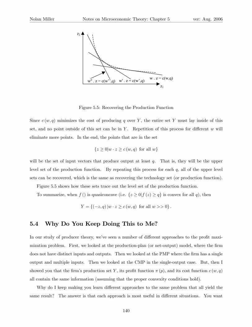
Nolan Miller Notes on Microeconomic Theory: Chapter 5 ver: Aug. 2006
z1
z2
w . z = c(w,q)w' . z = c(w’,q)w'' . z = c(w’’,q)
Figure 5.5: Recovering the Production Function
Since c (w, q) minimizes the cost of producing q over Y , the entire set Y must lay inside of this
set, and no point outside of this set can be in Y . Repetition of this process for different w will
eliminate more points. In the end, the points that are in the set
{z ≥ 0|w · z ≥ c (w, q) for all w}
will be the set of input vectors that produce output at least q. That is, they will be the upper
level set of the production function. By repeating this process for each q, all of the upper level
sets can be recovered, which is the same as recovering the technology set (or production function).
Figure 5.5 shows how these sets trace out the level set of the production function.
To summarize, when f () is quasiconcave (i.e. {z ≥ 0|f (z) ≥ q} is convex for all q), then
Y = {(−z, q) |w · z ≥ c (w, q) for all w >> 0} .
5.4 Why Do You Keep Doing This to Me?
In our study of producer theory, we’ve seen a number of different approaches to the profit maxi-
mization problem. First, we looked at the production-plan (or net-output) model, where the firm
does not have distinct inputs and outputs. Then we looked at the PMP where the firm has a single
output and multiple inputs. Then we looked at the CMP in the single-output case. But, then I
showed you that the firm’s production set Y , its profit function π (p), and its cost function c (w, q)
all contain the same information (assuming that the proper convexity conditions hold).
Why do I keep making you learn different approaches to the same problem that all yield the
same result? The answer is that each approach is most useful in different situations. You want
140
Nolan Miller Notes on Microeconomic Theory: Chapter 5 ver: Aug. 2006
to pick and choose the proper approach, depending on the problem you are working with.
The production-plan approach is useful for proving very general propositions, and necessary to
deal with situations where you don’t know which commodities will be inputs and which will be
outputs. This approach is widely used in the study of general equilibrium, where the output of
one industry is the input of another.
The CMP approach actually turns out to be very useful. We often have better data on the cost
a firm incurs than its production function. But, thanks to the recoverability results, we know that
the cost information contains everything we want to know about the firm. Thus the cost-function
approach can be very useful from an empirical standpoint.
In addition, recall that the PMP is not very useful for technologies with increasing returns to
scale. This is not so with the CMP. The CMP is perfectly well-defined as long as the production
function is quasiconcave, even if it exhibits increasing returns. Hence the CMP may allow us to
say things about firms when the PMP does not.
The CMP approach is useful for another reason. When the output price p is fixed, the firm’s
profit maximization problem in terms of the cost function is given by:
maxq
pq − c (w, q) .
However, this approach can also be used when the price the firm charges is not fixed. In particular,
suppose the price the firm can charge depends on the quantity it sells according to some function
P (q). The profit maximization problem can be written as
maxq
P (q) q − c (w, q) .
Thus our study of the cost function can also be used when the firm is not competitive, as in the
cases of monopoly and oligopoly. The other approaches to the PMP we have studied do not
translate well to environments where the firm is not a price taker.
5.5 The Geometry of Cost Functions
MWG Section 5.D relates the work we have done on cost functions to the diagrammatic approach
you may have studied in your previous micro classes. Although you should look at this section,
I’m not going to write everything. You should re-familiarize yourself with the concepts of total
cost, fixed cost, variable cost, marginal cost, average cost, etc. They will come in handy in the
future (although they are really intermediate micro topics).
141
Nolan Miller Notes on Microeconomic Theory: Chapter 5 ver: Aug. 2006
5.6 Aggregation of Supply
MWG summarizes this topic by saying, “If firms maximize profits taking prices as given, then the
production side of the economy aggregates beautifully.” To this let me add that the whole problem
with aggregation on the consumer side was with wealth effects. Since there is no budget constraint
here, there are no wealth effects, and thus there is no problem aggregating.
To aggregate supply, just add up the individual supply functions. Let there be m producers,
and let ym (p) be the net supply function for the mth firm. Aggregate supply can be written as:
yT (p) =MXm=1
ym (p) .
In fact, we can easily think of the aggregate production function as having been produced by
an aggregate producer. Define the aggregate production set Y T = Y 1+ ...+YM , where Y m is the
production set of the mth consumer. Thus Y T represents the opportunities that are available if all
sets are used together. Now, consider yT in Y T . This is an aggregate production plan. It can be
divided into parts, yT1, ..., yTM , where yTm ∈ Y m andP
m yTm = yT . That is, it can be divided
into parts, each of which lies in the production set of some firm. Fix a price vector p∗ and consider
the profit maximizing aggregate supply vector yT (p∗). The question we want to ask is this: Can
yT (p∗) be divided into parts yTm (p∗) such that yTm (p∗) = ym (p∗) andP
m yTm (p∗) = yT (p∗)? In
other words, is it the case that the profit maximizing production plan for the aggregate production
set is the same as would be generated by allowing each of the firms to maximize profit separately
and then adding up the profit-maximizing production plans for each firm? The answer is yes.
For all strictly positive prices, p >> 0, yT (p) =P
ym (p), and πT (p) =P
m πm (p). Thus the
aggregate profit obtained by each firm maximizing profit is the same as is attained by choosing the
profit-maximizing production plan from the aggregate production set.
The fact that production aggregates so nicely is a big help because aggregation tends to convexify
the production set. For example, see MWG 5.E.2. Even if each individual firm’s production
possibilities are non-convex, as in panel a), when you aggregate production possibilities and look
at the average production set, it becomes almost convex. Since non-convexities are a big problem
for economists, it is good to know that when you aggregate supply, the problems tend to go away.
142

Nolan Miller Notes on Microeconomic Theory: Chapter 5 ver: Aug. 2006
5.7 A First Crack at the Welfare Theorems
When economists talk about the fundamental theorems of welfare economics, they are really not
talking about welfare at all. What they are really talking about is efficiency. This is because,
traditionally, economists have not been willing to say what increases society’s “welfare,” since doing
so involves making judgments about how the benefits of various people should be compared. These
kind of judgments, which deal with equity or fairness, it is thought, are not the subject of pure
economics, but of public policy and philosophy.
However, while economists do not like to make equity judgments, we are willing to make the
following statement: Wasteful things are bad. That is, if you are doing something in a wasteful
manner, it would be better if you didn’t. That (unfortunately) is what we mean by welfare.
Actually, I’m giving economists too hard a time. The reason why we focus on wastefulness
(or efficiency) concerns is that while there will never be universal agreement on what is fair, there
can be universal agreement on what is wasteful. And as long as we believe that wastefulness is
bad, then anything that is fair can be made more fair by eliminating its wastefulness, at least in
principle.
Now let’s put this idea in practice. We will consider the question of whether profit maximizing
firms will choose production plans that are not wasteful. We will call a production plan y ∈ Y
efficient if there is no vector y0 ∈ Y such that y0i ≥ yi for all i, and y0 6= y. In other words, a
production plan is efficient if there is no other feasible production plan that could either: 1) produce
the same output using fewer inputs (i.e. y0j = yj and y0k > yk, where j denotes the output goods
and k denotes at least one of the input goods; y0k > yk when y0 uses less of input k, since y0k is
less negative than yk); or 2) produce greater output using the same amount of inputs (i.e. y0j > yj
and y0k = yk, where j denotes at least one of the output goods and k denotes all the input goods).
Thus, production plans that are not efficient are wasteful.
Efficient production plans are located on the firm’s transformation frontier. But, note that
there may be points on the transformation frontier that are not efficient, as is the case in Figure
5.6, where the transformation frontier has a horizontal segment. Points on the interior of the
horizontal part produce the same output as the point furthest to the right on the flat part, but use
more inputs. Hence they are not efficient (i.e., they are wasteful).
The first result, which is a version of the first fundamental theorem of welfare economics,
says that if a production plan is profit maximizing, then it is efficient. Formally, if there exists
143

Nolan Miller Notes on Microeconomic Theory: Chapter 5 ver: Aug. 2006
y y'
Figure 5.6: The Transformation Frontier
p >> 0 such that y (p) = y, then y is efficient. The reason for this is straightforward. Since the
profit maximizing point is on the transformation frontier, the only case we have to worry about is
when it lies on a flat part. But, of all of the points on a flat part, the one that maximizes profits
is the one that produces the given output using the fewest inputs, which means that it is also an
efficient point.
The second result deals with the converse question: Is it the case that any efficient point is
chosen as the profit maximizing point for some price vector? The answer to this case is, “Almost.”
If the production set is convex, then any efficient production plan y ∈ Y is the profit-maximizing
production plan for some price vector p ≥ 0. This result is known as the second fundamental
theorem of welfare economics. The reason why convexity is needed is illustrated in MWG
Figure 5.F.2. Basically, a point on a non-convex part of the transformation frontier can never be
chosen as profit-maximizing. However, any point that is on a convex part of the transformation
frontier can be chosen as profit-maximizing for the appropriate price vector. Also, notice that
p ≥ 0, not p >> 0. That is, some points, such as y in Figure 5.6, can only be chosen when some
of the prices are zero.
5.8 Constant Returns Technologies
As we saw earlier, technologies exhibiting increasing returns are a strange and special case. If
the technology exhibits increasing returns everywhere, then the firm will either choose to produce
nothing or the firm’s profits will grow without bound as it increases its scale of operations. Further,
if the firm exhibits increasing returns over a range of output, the firm will never choose to produce
144

Nolan Miller Notes on Microeconomic Theory: Chapter 5 ver: Aug. 2006
an output on the interior of this range. It will either choose the smallest or largest production plan
on the segment with increasing returns.
Because of the difficulties involved with increasing returns technologies, we tend to focus on
nonincreasing returns technologies. But, nonincreasing returns technologies can be divided into
two groups: technologies that exhibit decreasing returns and technologies that exhibit constant
returns.
In the single-output case, decreasing returns technologies are characterized by strictly concave
production functions. For example, a firm that uses machinery and labor to produce output may
have a production function of the Cobb-Douglas form:
q = f (zm, zl) = bz13mz
13l ,
where b > 0 is some positive real number (for the moment). This production function exhibits
decreasing returns to scale:
f (azm, azl) = b (azm)13 (azl)
13 = a
23 kzmzl = a
23 f (zm, zl) .
We can tell a story accounting for decreasing returns in this case. Suppose the firm has a
factory, and in it are some machines and some workers. At low levels of output, there is plenty
of room for the machines and workers. However, as output increases, additional machines and
workers are hired, and the factory begins to get crowded. Soon, the workers and machines begin
to interfere with each other, making them less productive. Eventually, the place gets so crowded
that nobody can get any work done. This is why the firm experiences decreasing returns to scale.
While the preceding story is realistic, notice that it depends on the fact that the size of the
factory is fixed. To put it another way, if the firm’s plant just kept growing as it hired more
workers and machines, they would never interfere with each other. Because of this, there would
be no decreasing returns.
The point of the argument I just gave is to point out that decreasing returns can usually be
traced back to some fixed input into the productive process that has not been recognized. In
this case, it was the fact that the firm’s factory was fixed. To illustrate, suppose that the b from
the previous production function really had to do with the fixed level of the plant. In particular,
suppose b = (zb)13 , where zb is the current size of the firm’s plant (building). Taking this into
account, the firm’s production function is really:
f (xm, xl, xb) = x13b x
13mx
13l ,
145
Nolan Miller Notes on Microeconomic Theory: Chapter 5 ver: Aug. 2006
and this production function exhibits constant returns to scale.
To paraphrase MWG on this point (bottom of p. 134), the production set Y represents techno-
logical possibilities, not limits on resources. If a firm’s current production plan can be replicated,
i.e., build an identical plant and fill it with identical machines and workers, then it should exhibit
constant returns to scale. Of course, it may not actually be possible to replicate everything in
practice, but it should be possible in theory. Because of this, it has been argued that decreasing
returns must reflect the underlying scarcity of an input into the productive process. Frequently
this is managerial know-how, special locations, or something else. However, if this factor could be
varied, the technology would exhibit constant returns. Because of this, many people believe that
constant returns technologies are the most important sub-category of convex technologies. And,
because of that, we’ll spend a little time looking at some of the peculiar features of constant returns
production functions.
Suppose that the firm produces output q from inputs labor (L) and capital (K) according to
q = f (K,L). If f () exhibits constant returns,
q = f (tK, tL) ≡ tf (K,L) , for any t > 0.
Since this holds for any t, it also holds for t = 1q . Making this substitution:
1 = f
µK
q,L
q
¶.
If we let Kq = k and L
q = l, then we can write the previous statement as:
f (k, l) = 1,
where k is the amount of capital used to produce one unit of output and l is the amount of labor
used to produce one unit of output.
To see why this is important, consider the following cost minimization problem:
minK,L
rK + sL
s.t. f (K,L) = q,
where r is the price of capital and s is the price of labor. We can rewrite this problem as:
minK,L
qrK + sL
q
s.t.1
qf (K,L) = 1,
146

Nolan Miller Notes on Microeconomic Theory: Chapter 5 ver: Aug. 2006
but 1qf (K,L) = f³Kq ,
Lq
´= f (k, l). Thus the CMP becomes:
min q (rk + sl)
s.t. f (k, l) = 1.
Thus if we want to solve the firm’s CMP, we can first find the cost-minimizing way to produce one
unit of output at the current input prices, and then replicate this production plan q times.
In other words, we can learn everything we want to know about the firm’s production function
by studying a single isoquant — in this case the unit isoquant.
As another special case of a constant returns technology, we can think of the situation where
the firm only has a finite number of alternative production plans. For example, suppose that it
can either produce 1 unit of output using 5 units of capital and 3 unit of labor or 2 units of capital
and 7 units of labor. Frequently we will call the different production plans in this environment
“activities.” Thus activity 1 is (5, 3) and activity 2 is (2, 7).
If the firm has the two activities above, then it can produce one unit of output using either
inputs (5, 3) or inputs (2, 7). But, we can also allow the firm to mix the two activities. Thus it
can also produce one unit of output by producing 0 ≤ a ≤ 1 units of output using activity 1 and
1 − a units of output using activity 2. Hence for a firm with these two activities available, the
firm’s unit isoquant consists of the curve:
(k, 3) when k > 5
a (5, 3) + (1− a) (2, 7) for a ∈ [0, 1]
(2, l) for l > 7.
Figure 5.7 depicts this unit isoquant. Note that the vertical and horizontal segments follow from
our assumption of free disposal. Also note that if we had more activities, we would begin to
trace out something that looks like the nicely differentiable isoquants we have been dealing with
all along. Thus differentiable isoquants can be thought of as the limit of having many activities
and the “convexification” process we did above.
As a final point, let me make a connection to something you might have seen in your macro
classes. Go back to:
q = f (tK, tL) ≡ tf (K,L) , for any t > 0.
Instead of dividing by q, as we did above, we can divide by the available labor, L. If we do this,
147

Nolan Miller Notes on Microeconomic Theory: Chapter 5 ver: Aug. 2006
(5,3)
(2,7)
k
L
q = 1
Figure 5.7: The Unit Isoquant
we get:q
L= f
µK
L, 1
¶.
Here we have a version of the production function that gives per capita output as a function of
capital. This is something that is useful in macro models. I just wanted to show you that this
formula, which you may have seen, is grounded in the production theory we have been studying.
5.9 Household Production Models
Now that we have studied both consumer and producer theories, we can begin to think about how
these parts fit together. Chapter 7 explores this topic at the level of the whole economy, but here
we start by looking at the individual household as the unit of both production and consumption.
In particular, we consider consumers who are able to produce one of the commodities using (at
least in part) their own labor. Consider, for example, a consumer who owns a small farm and has
preferences over leisure and consumption of the farm’s output, which we will call “food.” Labor
for the farm can either be provided by the farmer or by hiring labor from the market, and food
produced by the farm can either be consumed internally by the farmer or sold on the market. Thus
it appears that the farmer’s decision about how much leisure and food to consume is intertwined
with his decision about how much food to produce on the farm and how much labor to hire.
However, we will show that if the market for labor is complete, then the farmer’s production and
consumption decisions can be separated. The farmer can maximize utility by first choosing the
amount of total labor that maximizes profit from the farm and then deciding how much of the labor
he will provide himself.
148

Nolan Miller Notes on Microeconomic Theory: Chapter 5 ver: Aug. 2006
5.9.1 Agricultural Household Models with Complete Markets
Models of situations such as we’ve been talking about are known as Agricultural Household Models
(AHM). The version I’ll give you here is a simplification of the model in Bardhan and Udry,
Development Microeconomics, Chapter 2.
Consider a farm owner who can either work on the farm, work off the farm, or not work (leisure).
Similarly, he can use his farm land for his own farming, rent it to others to use, or not use it. In
addition, the farmer can buy additional labor from the market or rent additional land from the
market. Total output produced by the farm depends on the total land used and total labor used
on the farm.
We assume that the farmer faces a complete set of markets and that the buying and selling
prices for food, labor, and land are the same. Let p be the price of output, w be the price of labor
and r be the rental price of land.8
The farmer has utility defined over consumption of food and leisure:
u (c, l)
where c is consumption and l is leisure per person.
The total size of the output is given by
F (L,A)
where L is the total amount of labor employed on the farm and A is the total amount of land that
is cultivated.
The farmer owns a farm with AE acres. These acres can either be used on the farm or rented
to others on the market. Let AU be the number of acres used on the farm and AS be the number
of acres rented to (sold to) others. Since the farmer gets no utility from having idle land, it
is straightforward to show that all acres will either be used internally or rented to the market.
Similarly, the farmer has initial endowment of LE of labor. Let LU and LS be the number of units
of labor that are used on the farm and sold to the market, respectively. Thus we have two resource
constraints:
AE = AU +AS
LE = LU + LS + l.8The natural units are for w to be the price per day of labor and r to be the price per season of an acre of land.
149
Nolan Miller Notes on Microeconomic Theory: Chapter 5 ver: Aug. 2006
These constraints say that all land is either used internally or sold to the market, and all labor
is either used internally, sold to the market, or consumed as leisure.
Let AB and LB, respectively, be the number of units of land and labor bought from the market.
Total labor used on the farm is then given by:
L = LU + LB
and total land used on the farm is given by:
A = AU +AB.
The household’s utility maximization problem can be written as:
maxu (c, l)
s.t :
wLB + rAB ≤ p (F (L,A)− c) + wLS + rAS
L = LU + LB
A = AU +AB
l = LE − LU − LS
0 = AE −AU −AS.
The first constraint is a budget constraint. The left-hand side consists of expenditure on labor
(wLB) and land (rAB) purchased from the market. The right-hand side consists of net revenue
from selling the crop to the market (the price is p, and the amount sold is equal to total production
F (L,A) less the amount consumption internally, c), plus revenue from selling labor to the market
wLS and revenue from selling land to the market rAS. The remaining constraints are the definitions
of land and labor used on the farm and the resource constraints on available time and land.
Through simplification, the constraints can be rewritten as:
w (LB − LS) + r (AB −AS) ≤ p (F (L,A)− c)
L− LU = LB
l − LE + LU = −LS
A−AU = AB
AU −AE = −AS .
150
Nolan Miller Notes on Microeconomic Theory: Chapter 5 ver: Aug. 2006
or
w (L+ l − LE) + r (A−AE) ≤ p (F (L,A)− c)
or
wl + pc ≤ pF (L,A)−wL+wLE − rA+ rAE
or
wl + pc ≤ Π+ wLE + rAE
Π = pF (L,A)− wL− rA.
The last version says that the total expenditure on commodities, wl+ pc, must be less than the
profit earned by running the farm, Π, plus the value of the farmer’s initial endowment, wLE+rAE .
But, notice that L and A appear only on the right-hand side of the budget constraint. Because of
this, we can solve the farmer’s problem in two stages. First, solve
maxL,A
pF (L,A)−wL− rA
for the optimal total labor and land to be used on the farm. Second, solve the farmer’s utility
maximization problem:
maxl,c
u (c, l)
s.t. : wl + pc ≤ Π∗ +wLE + rAE
where
Π∗ = maxL,A
pF (L,A)− wL− rA
is the maximum profit that can be generated on the farm at prices p, w, and r.
What does this mean? Well, the variables l and c have to do with the farmer’s consumption
decisions. The variables L and A have to do with his production decisions. The essence of this
result says that if you want to solve the farmer’s overall utility maximization problem, you can
separate his production and consumption decisions. First, choose the production variables that
maximize the profit produced on the farm.9 Then, choose the consumption bundle that maximizes9There is some degeneracy in the solution to this problem. To see why, suppose the farmer owns 100 acres of
land and chooses to cultivate 80 acres himself. Based on the math of the problem, the farmer is indifferent between
using 80 acres of his own land and renting 20 on the outside market and, for example, renting all 100 acres of his
own land on the market and renting 80 different acres from the market. For simplicity, we’ll just assume that the
farmer first uses his own land and rents any remaining land to the market (or, if A > AE , that he uses all of his own
land and rents the remainder from the market).
151

Nolan Miller Notes on Microeconomic Theory: Chapter 5 ver: Aug. 2006
utility subject to the “ordinary” budget constraint, where wealth is the sum of maximized profit
and endowment wealth. To put it another way, the farmer has two separate decisions to make:
how much land and labor to use on the farm, and how much leisure and food to consume. These
two decisions can be made separately. In particular, the farmer can decide how much labor to use
on the farm without deciding how much of his own labor he should use on the farm. Similarly,
the farmer can decide how much food to produce without deciding how much food he, himself, is
going to consume.
The result stated in the previous paragraph is known as the separation property of the AHP:
When markets are complete, the production and consumption decisions of the household are sep-
arate from each other. The farmer chooses total labor and land in order to maximize profit, and
then chooses how much labor and land to consume as if in an ordinary UMP, where wealth is the
sum of maximized profit from production and endowment wealth.
The separation property is an implication of utility maximization and complete markets, and
it arises endogenously as an implication of the model. Completeness of markets plays a critical
role in the result. For our purposes, a market is complete if the farmer can buy or sell as much of
the commodity as he wants at a particular price that is the same regardless of whether the farmer
buys or sells. A market can fail to be complete if either the price at which someone buys an item
is different than the price at which he sells the item, or if there are limits on the quantity that can
be bought or sold of an item.10
A graphical illustration of the separation property may help. For illustration (because three
dimensional graphs are hard to draw), we will assume that there is no market for land. The farmer
has AE = A∗ acres of land, and uses them all on the farm. The first stage of the optimization
problem is to choose the amount of labor to use on the farm. This is done by maximizing the
profit earned on the farm, pc − wL, subject to the constraint that c = F (L,A∗). This profit
maximization problem is illustrated in Figure 5.8. Thus the first stage in the farmer’s decision
results in L∗ units of labor being used on the farm. When this amount of labor is used, the farm’s
profit is given by the level of the solid black isoprofit line at L∗. The equation of this line is given
by c = F (L∗, A∗) + wp (LU + LS).11 If the farmer chooses to work more than L∗ by selling some
10One of the chief “market failures” in developing economies is incompleteness of labor markets. It is often
impossible to buy labor regardless of the price offered because it is costly for the people who have jobs to find the
people who are willing to work.11This isoprofit line makes intuitive sense if you think about it as a budget line. Consumption equals the total
product of the farm plus the value of labor provided by the farmer, normalized to the units of consumption (w/p).
152

Nolan Miller Notes on Microeconomic Theory: Chapter 5 ver: Aug. 2006
Isoprofit Lines
Profitincreases
Profit ismaximized
F(L,A*)
L* labor
output
Figure 5.8: Profit Maximization
of his labor on the market, he moves to the right along the solid isoprofit line and increases the
amount of wealth he has for consumption. If he chooses to work less than L∗, he moves to the left
along the solid isoprofit line and decreases the wealth he has available for consumption.
In the second stage the farmer chooses how much labor he will provide. This is found by
maximizing utility subject to the constraint that total spending satisfy the budget constraint c ≤
F (L∗, A∗) + wp (LU + LS) (which we know will bind). The solution is depicted in Figure 5.9. As
illustrated in the figure, L∗ < LE. Under the natural assumption that if the total labor used on
the farm is less than the farmer’s endowment of labor, he will buy no labor from the market, the
farmer’s choice of labor used on the farm (L∗U ), labor sold to the market (L∗S), and leisure (l
∗) are
as shown in the diagram.
You can think of the parts of Figure 5.9 as evolving as follows. First, the farmer chooses how
much labor, L∗, to use on the farm. This quantity is chosen in order to maximize profit without
regard to how much of L∗ will be provided by the farmer, himself, and how much will be hired from
the market. Next, the farmer chooses how much of his own leisure to provide as labor, given that,
in addition to any labor income he might earn, he will also have the profit from the farm to use to
purchase the consumption good. Thus in the second stage the farmer chooses labor according to
the budget set defined by the farm’s maximized isoprofit line.
Generally speaking, the separation property will not hold if markets are sufficiently incomplete.
Notice that in the model we presented, the separation result would continue to hold if either the
market for labor or land were incomplete (i.e., labor or land could not be traded), but not both.
However, if multiple markets were incomplete, the separation result would fail.
153

Nolan Miller Notes on Microeconomic Theory: Chapter 5 ver: Aug. 2006
Profit ismaximized
F(L,A*)
L* labor
output /consumption
Set of affordablelabor/consumptionpairs (budget line)
utility increases
LE
u-max point
LU* l*LS
*
Figure 5.9: Separation Property
Suppose there is no market for land (that is, A = AE) and there is an upper bound on how
much labor the household can sell to the market (that is, LS ≤M). The farmer’s problem is given
by:
maxu (c, l)
s.t :
wLB ≤ p (F (L,AE)− c) + wLS
l = LE − LS − LU
L = LB + LU
LS ≤ M.
This version of the model is the same as the complete market version except that we have eliminated
the market for land and added the constraint that the amount of labor sold on the market must
be less than M .
The optimal solution to this problem takes one of two forms. If, in the perfect markets version
of the problem L∗S < M , then the solution in the incomplete markets case is the same as in the
complete markets case. On the other hand, if L∗ > M in the complete markets case, then the
farmer is limited by the incomplete market and must choose L∗S =M . Because of this, separation
will fail to hold. Intuitively, this is because if separation holds the farmer can first decide how
154

Nolan Miller Notes on Microeconomic Theory: Chapter 5 ver: Aug. 2006
much labor to use on the farm and then decide how much of his own labor to use. So, suppose
the farmer would choose to operate a small farm (i.e., one that uses a small amount of labor). If
markets are complete, he can then sell his surplus labor. But, if markets are not complete, the
farmer will not be able to sell the surplus labor. Because of this, he will consume some of the
excess as leisure, but he will also use some of it as additional labor on his own farm. Thus the
optimal amount of labor to use on the farm will be affected by the amount of labor that the farmer
can sell. Separation does not hold.
Formally, when the constraint on use of the labor market binds, the problem becomes:
maxu (c, l)
s.t : pc = pF (LE −M − l, AE) +wM
and the optimum is found at the point of tangency between the production function F and the
utility function u (c, l). This will generally not be the same point as the farmer would select if
markets were complete.
Figure 5.10 illustrates the farmer’s problem when the market for labor is incomplete. Suppose
that in the absence of labor market imperfections, the farmer would like to sell a lot of labor:
L∗S > M. In this case, the constraint will bind, and leisure is given by: l = LE − LU −M . Thus
the consumer can no longer independently choose LU and l. Setting one determines the other.
So, consider three alternative values of LU : L1U , L2U , and L3U . L1U is the value of LU that
maximizes profit from the farm. However, notice that because of the credit market imperfection,
the farmer is only able to move along the profit line to the point labeled (1), where he works L1U
hours at home, sells M hours of labor, and consumes l = LE −M − L1U hours as leisure. If the
farmer increases labor usage to L2U , he changes the farm’s profit, and so as he sells labor he moves
along the new profit line to the point labeled (2), again by selling the maximum number of labor
hours. Notice that point 2 involves more consumption but less leisure than point 1. Similarly, if
the farmer works L3U units of labor at home, then he can move along the new profit line to point
(3). And, point 3 offers more consumption and less leisure than either point 2 or point 3.
Whether the farmer prefers point 1, 2, or 3 will depend on the shape of his isoquants, as
illustrated in Figure 5.11. If they are relatively flat, then the consumer will prefer more consumption
and less leisure: point 3 will be the best. However, if they are steep, then the farmer will prefer more
leisure and less consumption - point 1 will be the best. Finally, for more intermediate preferences,
point 2 may be the best. In any case, since the optimal point depends on the shape of the farmer’s
155

Nolan Miller Notes on Microeconomic Theory: Chapter 5 ver: Aug. 2006
LU1 + M LU
2 + M LU3 + MLU
1 LU2 LU
3
1
2
3c
LE
Figure 5.10: Imperfect Labor Markets
utility isoquants and the shape of the production function, he will no longer be able to separate his
production and consumption decisions.
156
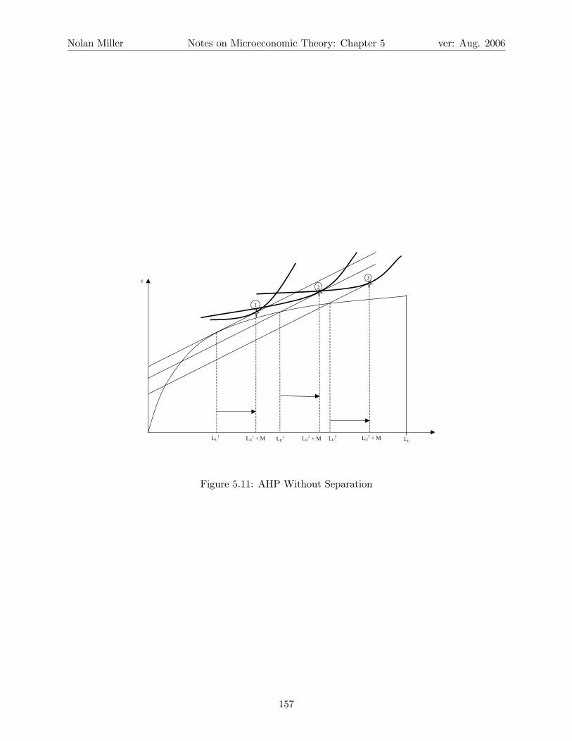
Nolan Miller Notes on Microeconomic Theory: Chapter 5 ver: Aug. 2006
LU1 + M LU
2 + M LU3 + MLU
1 LU2 LU
3
1
2
3c
LE
Figure 5.11: AHP Without Separation
157

Chapter 6
Choice Under Uncertainty
Up until now, we have been concerned with choice under certainty. A consumer chooses which
commodity bundle to consume. A producer chooses how much output to produce using which mix
of inputs. In either case, there is no uncertainty about the outcome of the choice.
We now turn to considering choice under uncertainty, where the objects of choice are not
certainties, but distributions over outcomes. For example, suppose that you have a choice between
two alternatives. Under alternative A, you roll a six-sided die. If the die comes up 1, 2, or 3, you
get $1000. If it comes up 4, 5, or 6, you lose $300. Under alternative B, you choose a card from
a standard 52 card deck. If the card you choose is black, you pay me $200. If it is a heart, you
get a free trip to Bermuda. If it is a diamond, you have to shovel the snow off of my driveway all
winter.
If I were to ask you whether you preferred alternative A or alternative B, you could probably
tell me. Indeed, if I were to write down any two random situations, call them L1 and L2, you could
probably tell me which one you prefer. And, there is even the possibility that your preferences
would be complete, transitive (i.e., rational), and continuous. If this is true then I can come up
with a utility function representing your preferences over random situations, call it U (L), such that
L1 is strictly preferred to L2 if and only if U (L1) > U (L2). Thus, without too much effort, we can
extend our standard utility theory to utility under uncertainty. All we need is for the consumer
to have well defined preferences over uncertain alternatives.
Now, recall that I said that much of what we do from a modeling perspective is add structure
to people’s preferences in order to be able to say more about how they behave. In this situation,
what we would like to be able to do is say that a person’s preferences over uncertain alternatives
158

Nolan Miller Notes on Microeconomic Theory: Chapter 6 ver: Aug. 2006
should be able to be expressed in terms of the utility the person would assign to the outcome if
it were certain to occur, and the probability of that outcome occurring. For example, suppose
we are considering two different uncertain alternatives, each of which offers a different distribution
over three outcomes: I buy you a trip to Bermuda, you pay me $500, or you paint my house. The
probability of each outcome under alternatives A and B are given in the following table:
Bermuda -$500 Paint my house
A .3 .4 .3
B .2 .7 .1
What we would like to be able to do is express your utility for these two alternatives in terms
of the utility you assign to each individual outcome and the probability that they occur. For
example, suppose you assign value uB to the trip to Bermuda, um to paying me the money, and up
to painting my house. It would be very nice if we could express your utility for each alternative
by multiplying each of these numbers by the probability of the outcome occurring, and summing.
That is:
U (A) = 0.3uB + 0.4um + 0.3up
U (B) = 0.2uB + 0.7um + 0.1up.
Note that if this were the case, we could express the utility of any distribution over these outcomes
in the same way. If the probabilities of Bermuda, paying me the money, and painting my house
are pB, pm, and pp, respectively, then the expected utility of the alternative is
pBuB + pmum + ppup.
This would be very useful, since it would allow us to base our study of choice under uncertainty on
a study of choice over certain outcomes, extended in a simple way.
However, while the preceding equation, known as an expected utility form, is useful, it is
not necessarily the case that a consumer with rational preferences over uncertain alternatives will
be such that those alternatives can be represented in this form. Thus the question we turn to
first is what additional structure we have to place on preferences in order to ensure that a person’s
preferences can be represented by a utility function that takes the expected utility form. After
identifying these conditions, we will go on to show how utility functions of the expected utility form
can be used to study behavior under uncertainty, and draw testable implications about people’s
behavior that are not implied by the standard approach.
159

Nolan Miller Notes on Microeconomic Theory: Chapter 6 ver: Aug. 2006
6.1 Lotteries
In our study of consumer theory, the object of choice was a commodity bundle, x. In producer
theory, the object of choice was a net input vector, y. In studying choice under uncertainty, the
basic object of choice will be a lottery. A lottery is a probability distribution over a set of possible
outcomes.
Suppose that there are N possible outcomes, denoted by a1, ..., aN . Let A = {a1, ..., aN} denote
the set of all possible outcomes. A simple lottery consists of an assignment of a probability to
each outcome. Thus a simple lottery is a vector L = (p1, ..., pN) such that pn ≥ 0 for n = 1, ..., N ,
andP
n pn = 1.
A compound lottery is a lottery whose prizes are other lotteries. For example, suppose that I
ask you to flip a coin. If it comes up heads, you roll a die, and I pay you the number of dollars that
it shows. If the die comes up tails, you draw a random number between 1 and 10 and I pay you that
amount of dollars. The set of outcomes here is A = (1, 2, 3, 4, 5, 6, 7, 8, 9, 10) . The coin flip is then a
lottery whose prizes are the lotteries¡16 ,16 ,16 ,16 ,16 ,16 , 0, 0, 0, 0
¢and
¡110 ,
110 ,
110 ,
110 ,
110 ,
110 ,
110 ,
110 ,
110 ,
110
¢.
Thus the coin flip represents a compound lottery. Notice that since the coin comes up heads or
tails with probability 12 each, the compound lottery can be reduced to a simple lottery:
1
2
µ1
6,1
6,1
6,1
6,1
6,1
6, 0, 0, 0, 0
¶+1
2
µ1
10,1
10,1
10,1
10,1
10,1
10,1
10,1
10,1
10,1
10
¶=
µ2
15,2
15,2
15,2
15,2
15,2
15,1
20,1
20,1
20,1
20
¶,
where the final vector gives the probability of each outcome before the coin is flipped.
Generally, a compound lottery can be represented as follows. Suppose that there areK lotteries,
denoted by L1, ..., LK . Let Q be a lottery whose prizes are the lotteries L1, ..., LK . That is, suppose
that lottery Q awards the prize Lk with probability qk. So, you can think of a compound lottery as
a two-stage lottery. In the first stage, which lottery Lk you play in the second stage is determined.
In the second stage, you play lottery Lk.
So, we call Q a compound lottery. It assigns probability qk to Lk, where qk ≥ 0 andP
k qk = 1.
If pkn is the probability that Lk assigns to outcome n, this compound lottery can be reduced to a
simple lottery where
pn =Xk
qkpkn
is the probability of outcome n occurring. That is, pn gives the probability of outcome n being the
final outcome of the compound lottery before any of the randomizations have occurred.
160

Nolan Miller Notes on Microeconomic Theory: Chapter 6 ver: Aug. 2006
If L and L0 are lotteries, a compound lottery over these two lotteries can be represented as
aL+ (1− a)L0, where 0 ≤ a ≤ 1 is the probability of lottery L occurring.
6.1.1 Preferences Over Lotteries
We begin by building up a theory of rational preferences over lotteries. Once we do that, we’ll
know that there is a utility function that represents those preferences (under certain conditions).
We’ll then go on to ask whether those preferences can be represented by a utility function of the
expected utility form.
Let L be the set of all possible lotteries. Thus L is like X from consumer theory, the set of all
possible consumption bundles. We want our consumer to have rational preferences over lotteries.
So, suppose that the relation % represents strict preferences over lotteries, and suppose that these
preferences are rational, i.e., complete and transitive.
We will also assume that the consumer’s preferences are consequentialist. Basically, this
means that consumers care only about the distribution over final outcomes, not whether this dis-
tribution comes about as a result of a simple lottery, or a compound lottery. In other words,
the consumer is indifferent between any two compound lotteries that can be reduced to the same
simple lottery. This property is often called reduction of compound lotteries.1 Because of
the reduction property, we can confine our attention to the set of all simple lotteries, and from now
on we will let L be the set of all simple lotteries.
The other requirement we needed for preferences to be representable by a utility function was
continuity. In consumer theory, continuity meant that you could not pass from the lower level set
of a consumer’s utility function to the upper level set without passing through the indifference set.
Something similar is involved with continuity here, but what we are interested in is continuity in
probabilities.
Suppose that L Â L0. The essence of continuity is that adding a sufficiently small probability
of some other lottery, L00, to L should not reverse this preferences. That is:
if L Â L0, then L Â (1− a)L0 + aL00 for some a > 0.
1Another way to think about the reduction property is that we’re assuming there is no process-oriented utility.
Consumers do not enjoy the process of the gamble, only the outcome, eliminating the “fun of the gamble” in settings
like casinos.
161
Nolan Miller Notes on Microeconomic Theory: Chapter 6 ver: Aug. 2006
Formally, % on L is continuous if for any L, L0, and L00, and any a ∈ (0, 1), the sets:
©a ∈ (0, 1) |L % (1− a)L0 + aL00
ªand ©
a ∈ (0, 1) | (1− a)L0 + aL00 % Lª
are closed.
Continuity is mostly a technical assumption needed to get the existence of a utility function.
But, notice that its validity is less compelling than it was in the certainty case. For example,
suppose L is a trip to Bermuda and L0 is $3000, and that you prefer L0 to L. Now suppose
we introduce L00, which is violent, painful, death. If preferences are continuous, then the trip to
Bermuda should also be less preferred than $3000 with probability 1− a and violent painful death
with probability a, provided that a is sufficiently small. For many people, there is no probability
a > 0 such that this would be the case, even though when a = 0, L0 is preferred to L.
If the consumer has rational, continuous preferences over L, we know that there is a utility
function U () such that U () represents those preferences. In order to get a utility function of the
expected utility form that represents those preferences, the consumer’s preferences must also satisfy
the independence axiom.
The preferences relation % on L satisfies the independence axiom if for all L,L0, and L00 and
a ∈ (0, 1), L % L0 if and only if aL+ (1− a)L00 % aL0 + (1− a)L00.
The essence of the independence axiom is that outcomes that occur with the same probability
under two alternatives should not affect your preferences over those alternatives. For example,
suppose that I offer you the choice between the following two alternatives:
L : $5 with probability1
5, 0 with probability
4
5
L0 : $12 with probability1
10, 0 with probability
9
10.
Suppose you prefer L to L0. Now consider the following alternative. I flip a coin. If it comes up
heads, I offer you the choice between L and L0. If it comes up tails, you get nothing. What the
independence axiom says is that if I ask you to choose either L or L0 before I flip the coin, your
preference should be the same as it was when I didn’t flip the coin. That is, if you prefer L to L0,
you should also prefer 12L+120 % 1
2L0+ 1
20, where 0 is the lottery that gives you 0 with probability
1.
162
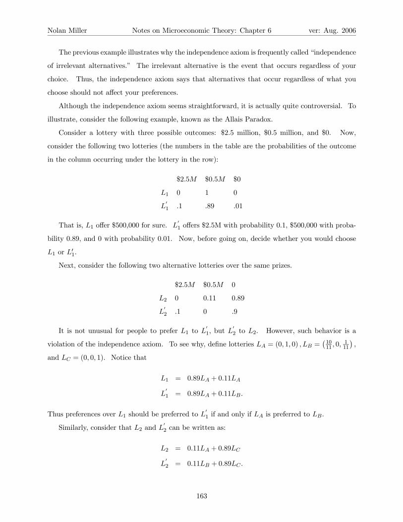
Nolan Miller Notes on Microeconomic Theory: Chapter 6 ver: Aug. 2006
The previous example illustrates why the independence axiom is frequently called “independence
of irrelevant alternatives.” The irrelevant alternative is the event that occurs regardless of your
choice. Thus, the independence axiom says that alternatives that occur regardless of what you
choose should not affect your preferences.
Although the independence axiom seems straightforward, it is actually quite controversial. To
illustrate, consider the following example, known as the Allais Paradox.
Consider a lottery with three possible outcomes: $2.5 million, $0.5 million, and $0. Now,
consider the following two lotteries (the numbers in the table are the probabilities of the outcome
in the column occurring under the lottery in the row):
$2.5M $0.5M $0
L1 0 1 0
L01 .1 .89 .01
That is, L1 offer $500,000 for sure. L01 offers $2.5M with probability 0.1, $500,000 with proba-
bility 0.89, and 0 with probability 0.01. Now, before going on, decide whether you would choose
L1 or L01.
Next, consider the following two alternative lotteries over the same prizes.
$2.5M $0.5M 0
L2 0 0.11 0.89
L02 .1 0 .9
It is not unusual for people to prefer L1 to L01, but L
02 to L2. However, such behavior is a
violation of the independence axiom. To see why, define lotteries LA = (0, 1, 0) , LB =¡1011 , 0,
111
¢,
and LC = (0, 0, 1). Notice that
L1 = 0.89LA + 0.11LA
L01 = 0.89LA + 0.11LB.
Thus preferences over L1 should be preferred to L01 if and only if LA is preferred to LB.
Similarly, consider that L2 and L02 can be written as:
L2 = 0.11LA + 0.89LC
L02 = 0.11LB + 0.89LC .
163

Nolan Miller Notes on Microeconomic Theory: Chapter 6 ver: Aug. 2006
Thus if this person satisfies the independence axiom, L2 should be preferred to L02 whenever LA is
preferred to LB, which is the same as in the L1 vs. L01 case above. Hence if L1 is preferred to L
01,
then L2 should also be preferred to L02.
Usually, about half of the people prefer L1 to L01 but L
02 to L2. Does this mean that they
are irrational? Not really. What it means is that they do not satisfy the independence axiom.
Whether or not such preferences are irrational has been a subject of debate in economics. Some
people think yes. Others think no. Some people would argue that if your preferences don’t satisfy
the independence axiom, it’s only because you don’t understand the problem. And, once the
nature of your failure has been explained to you, you will agree that your behavior should satisfy
the independence axiom and that you must have been mistaken or crazy when it didn’t. Others
think this is complete nonsense. Basically, the independence axiom is a source of great controversy
in economics. This is especially true because the independence axiom leads to a great number of
paradoxes like the Allais paradox mentioned earlier.
In the end, the usefulness of the expected utility framework that we are about to develop usually
justifies its use, even though it is not perfect. A lot of the research that is currently going on is
trying to determine how you can have an expected utility theory without the independence axiom.
6.1.2 The Expected Utility Theorem
We now return to the question of when there is a utility function of the expected utility form that
represents the consumer’s preferences. Recall the definition:
Definition 9 A utility function U (L) has an expected utility form if there are real numbers u1, ..., uN
such that for every simple lottery L = (p1, ..., pN ),
U (L) =Xn
pnun.
The reduction property and the independence axiom combine to show that utility function
U (L) has the expected utility form if and only if it is linear, meaning it satisfies the
property:
U
ÃKXk=1
tkLk
!=
KXk=1
tkU (Lk) (6.1)
for any K lotteries. To see why, note that we need to show this in “two directions” - first, that
the expected utility form implies linearity; then, that linearity implies the expected utility form.
164

Nolan Miller Notes on Microeconomic Theory: Chapter 6 ver: Aug. 2006
1. Suppose that U (L) has the expected utility form. Consider the compound lotteryPK
k=1 tkLk.
U
ÃKXk=1
tkLk
!=Xn
un
ÃKXk=1
tkpkn
!=
KXk=1
tk
ÃXn
unpkn
!=
KXk=1
tkU (Lk) .
So, it is linear.
2. Suppose that U (L) is linear. Let Ln be the lottery that awards outcome an with probability
1. Then
U (L) = U
ÃXn
pnLn
!=Xn
pnU (Ln) =
Xn
pnun.
So, it has the expected utility form.
Thus proving that a utility function has the expected utility form is equivalent to proving it is
linear. We will use this fact momentarily.
The expected utility theorem says that if a consumer’s preferences over simple lotteries
are rational, continuous, and exhibit the reduction and independence properties, then there is a
utility function of the expected utility form that represents those preferences. The argument is by
construction. To make things simple, suppose that there is a best prize, aB, and a worst prize, aW ,
among the prizes. Let LB be the “degenerate lottery” that puts probability 1 on aB occurring,
and LW be the degenerate lottery that puts probability 1 on aW . Now, consider some lottery, L,
such that LB Â L Â LW . By continuity, there exists some number, aL, such that
aLLB + (1− aL)L
W ∼ L.
We will define the consumer’s utility function as U (L) = aL as defined above, and note that
U¡LB¢= 1 and U
¡LW
¢= 0. Thus the utility assigned to a lottery is equal to the probability
put on the best prize in a lottery between the best and worst prizes such that the consumer is
indifferent between L and aLLB + (1− aL)L
W .
In order to show that U (L) takes the expected utility form, we must show that:
U¡tL+ (1− t)L0
¢= taL + (1− t) aL0 .
If this is so, then U () is linear, and thus we know that it can be represented in the expected utility
form. Now, L ∼ aLLB + (1− aL)L
W , and L0 ∼ aL0LB + (1− aL0)L
W . Thus:
U¡tL+ (1− t)L0
¢= U
¡t¡aLL
B + (1− aL)LW¢+ (1− t)
¡aL0L
B + (1− aL0)LW¢¢
165

Nolan Miller Notes on Microeconomic Theory: Chapter 6 ver: Aug. 2006
by the independence property. By the reduction property:
= U¡(taL + (1− t) aL0)L
B + (1− ((taL + (1− t) aL0)))LW¢
and by the definition of the utility function:
= taL + (1− t) aL0 .
This proves that U () is linear, and so we know that U () can be written in the expected utility
form.2
I’m not going to write out the complete proof. However, I am going to write out the expected
utility theorem.
Expected Utility Theorem: Suppose that rational preference relation % is continuous and
satisfies the reduction and independence axioms on the space of simple lotteries L. Then % admits
a utility function U (L) of the expected utility form. That is, there are numbers u1, ..., uN such
that U (L) =PN
n=1 pLnun, and for any two lotteries,
L % L0 if and only if U (L) ≥ U¡L0¢.
Note the following about the expected utility theorem:
1. The expected utility theorem says that under these conditions, there is one utility function,
call it U (L) , of the expected utility form that represents these preferences.
2. However, there may be other utility functions that also represent these preferences.
3. In fact, any monotone transformation of U () will also represent these preferences. That is,
let V () be a monotone transformation, then V (U (L)) = V¡P
n pLnun
¢also represents these
preferences.
4. However, it is not necessarily the case that V (U (L)) can be written in the expected utility
form. For example, v = eu is a monotone transformation, but there is no way to write
V (U (L)) = exp¡P
n pLnun
¢in the expected utility form.
5. But, there are some types of transformations that can be applied to U () such that V (U ())
also has the expected utility form. It can be shown that the transformed utility function also
has the expected utility form if and only if V () is linear. This is summarized as follows:
2This is not a formal proof, but it captures the general idea. There are some technical details that must be
addressed in the formal proof, but you can read about these in your favorite micro text.
166

Nolan Miller Notes on Microeconomic Theory: Chapter 6 ver: Aug. 2006
The Expected Utility Form is preserved only by positive linear transformations. If
U () and V () are utility functions representing %, and U () has the expected utility form, then V ()
also has the expected utility form if and only if there are numbers a > 0 and b such that:
U (L) = aV (L) + b.
In other words, the expected utility property is preserved by positive linear (affine) transformations,
but any other transformation of U () does not preserve this property.
MWG calls the utility function of the expected utility form a von-Neumann-Morgenstern
(vNM) utility function, and I’ll adopt this as well. That said, it is important that we do not
confuse the vNM utility function, U (L) , with the numbers u1, ..., uN associated with it.3
An important consequence of the fact that the expected utility form is preserved only by positive
linear transformations is that a vNM utility function imposes cardinal significance on utility. To
see why, consider the utility associated with four prizes, u1, u2, u3, and u4, and suppose that
u1 − u2 > u3 − u4.
Suppose we apply a positive linear transformation to these numbers:
vn = aun + b.
Then
v1 − v2 = au1 + b− (au2 + b) = a (u1 − u2)
> a (u3 − u4) = au3 + b− (au4 + b) = v3 − v4.
Thus v1 − v2 > v3 − v4 if and only if u1 − u2 > u3 − u4. And, since any utility function of the
expected utility form that represents the same preferences will exhibit this property, differences in
utility numbers are meaningful. The numbers assigned by the vNM utility function have cardinal
significance. This will become important when we turn to our study of utility for money and risk
aversion, which we do next.
6.1.3 Constructing a vNM utility function
Let A = {a1, ..., aN} denote the set of prizes. Suppose that aN is the best prize and a1 is the worst
prize. We are going to show how to construct numbers u1, ..., uN that make up a utility function
with the expected utility form that represents preferences over these prizes.3Later, when we allow for a continuum of prizes (such as monetary outcomes), the numbers u1, ..., uN become the
function u (x), and we’ll call the lowercase u (x) function the Bernoulli utility function.
167

Nolan Miller Notes on Microeconomic Theory: Chapter 6 ver: Aug. 2006
First, we are going to arbitrarily choose uN = 1 and u1 = 0. Why? Because we can.
Remember, the point here is to construct a utility function that has the expected utility form. We
could just as easily do it for arbitrary specifications of uN and u1, but this is notationally a bit
simpler.
Now, for each prize ai, define ui to be the probability such that the decision maker is indifferent
between prize ai for sure and a lottery that offers aN with probability ui and a1 with probability
1−ui. Let’s refer to the lottery that offers prize aN with probability ui and prize a1 with probability
(1− ui) lottery Si. So, ui’s are between 0 and 1. Notice that if we specify the numbers in this
way it makes sense that uN = 1 and u1 = 0, since the decision maker should be indifferent between
the best prize for sure and a lottery that offers the best prize with probability u1 = 1, etc.
This gives us a way of defining numbers ui. Now, we want to argue that this way of defining
the ui’s, combined with consequentialism (reduction of compound lotteries) and Independence of
Irrelevant alternatives yields a utility function that looks like U (L) =P
piui.
So, consider lottery L = (p1, ..., pN). This lottery offers prize ai with probability pi. But, we
know that the decision maker is indifferent between ai for sure and a lottery that offers prize aN
with probability ui and price a1 with probability 1−ui. Thus, using IIA, we know that the decision
maker is indifferent between lottery L and a compound lotter in which, with probability pi, the
decision maker faces another lottery: uN with probability ui and u1 with probability 1− ui. This
lottery is depicted as L0 in the following diagram. Note that L0 only has two distinct prizes: aN
and a1. By reduction of compound lotteries, we can combine the total probability of each outcome,
making an equivalent simple lottery, L00. The utility for lottery L00 is (P
piui)uN+(1−P
piui)u1.
Since uN = 1 and u1 = 0, this gives that U (L) = U (L0) = U (L00) =P
piui, which is what we
wanted to show. Defining utility in this way gives us a representation with the expected utility
form.
6.2 Utility for Money and Risk Aversion
The theory of choice under uncertainty is most frequently applied to lotteries over monetary out-
comes. The easiest way to treat monetary outcomes here is to let x be a continuous variable
representing the amount of money received. With a finite number of outcomes, assign a number
un to each of the N outcomes. We could also do this with the continuous variable, x, just by
letting ux be the number assigned to the lottery that assigns utility x with probability 1. In this
168

Nolan Miller Notes on Microeconomic Theory: Chapter 6 ver: Aug. 2006
p1
a1
p2
p3
p4
a2
a3
a4
p1
p2
p3
p4
u1
u2
u3
u4
a1
aN
a1
aN
a1
aN
a1
aN
aN
a1
Σ pi ui
1- Σ pi ui
IIA
Reduction of compound lotteries
L L'
L''
Figure 6.1:
169
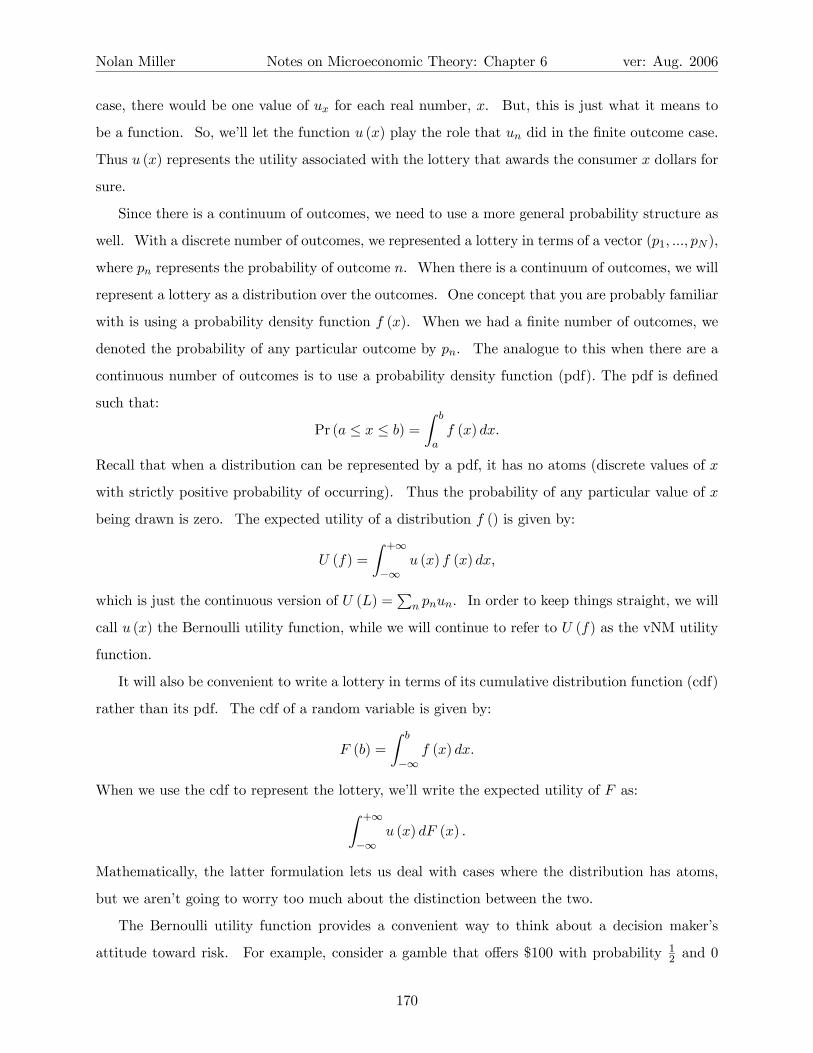
Nolan Miller Notes on Microeconomic Theory: Chapter 6 ver: Aug. 2006
case, there would be one value of ux for each real number, x. But, this is just what it means to
be a function. So, we’ll let the function u (x) play the role that un did in the finite outcome case.
Thus u (x) represents the utility associated with the lottery that awards the consumer x dollars for
sure.
Since there is a continuum of outcomes, we need to use a more general probability structure as
well. With a discrete number of outcomes, we represented a lottery in terms of a vector (p1, ..., pN ),
where pn represents the probability of outcome n. When there is a continuum of outcomes, we will
represent a lottery as a distribution over the outcomes. One concept that you are probably familiar
with is using a probability density function f (x). When we had a finite number of outcomes, we
denoted the probability of any particular outcome by pn. The analogue to this when there are a
continuous number of outcomes is to use a probability density function (pdf). The pdf is defined
such that:
Pr (a ≤ x ≤ b) =
Z b
af (x) dx.
Recall that when a distribution can be represented by a pdf, it has no atoms (discrete values of x
with strictly positive probability of occurring). Thus the probability of any particular value of x
being drawn is zero. The expected utility of a distribution f () is given by:
U (f) =
Z +∞
−∞u (x) f (x) dx,
which is just the continuous version of U (L) =P
n pnun. In order to keep things straight, we will
call u (x) the Bernoulli utility function, while we will continue to refer to U (f) as the vNM utility
function.
It will also be convenient to write a lottery in terms of its cumulative distribution function (cdf)
rather than its pdf. The cdf of a random variable is given by:
F (b) =
Z b
−∞f (x) dx.
When we use the cdf to represent the lottery, we’ll write the expected utility of F as:Z +∞
−∞u (x) dF (x) .
Mathematically, the latter formulation lets us deal with cases where the distribution has atoms,
but we aren’t going to worry too much about the distinction between the two.
The Bernoulli utility function provides a convenient way to think about a decision maker’s
attitude toward risk. For example, consider a gamble that offers $100 with probability 12 and 0
170

Nolan Miller Notes on Microeconomic Theory: Chapter 6 ver: Aug. 2006
with probability 12 . Now, if I were to offer you the choice between this lottery and c dollars for
sure, how small would c have to be before you are willing to accept the gamble?
The expected value of the gamble is 12100 +
120 = 50. However, if offered the choice between
50 for sure and the lottery above, most people would choose the sure thing. It is not until c is
somewhat lower than 50 that many people find themselves willing to accept the lottery. For me,
I think the smallest c for which I am willing to accept the gamble is 40. The fact that 40 < 50
captures the idea that I am risk averse. My expected utility from the lottery is less than the
utility I would receive from getting the expected value of the gamble for sure. The minimum
amount c such that I would accept the gamble instead of the sure thing is known as the certainty
equivalent of the gamble, since it equals the certain amount of money that offers the same utility
as the lottery. The difference between the expected value of the lottery, 50, and my certainty
equivalent, 40, is known as my risk premium, since I would in effect be willing to pay somebody
10 to take the risk away from me (i.e. replace the gamble with its expected value).
Formally, let’s define the certainty equivalent. Let c (F, u) be the certainty equivalent for a
person with Bernoulli utility function u facing lottery F , defined according to:
u (c (F, u)) =
Zu (x) dF (x)
Although generally speaking people are risk averse, this is a behavioral postulate rather than
an assumption or implication of our model. But, people need not be risk averse. In fact, we can
divide utility functions into four classes:
1. Risk averse. A decision maker is risk averse if the expected utility of any lottery, F , is not
more than the utility of the getting the expected value of the lottery for sure. That is, if:Zu (x) dF (x) ≤ u
µZxdF (x)
¶for all F.
(a) If the previous inequality is strict, we call the decision maker strictly risk averse.
(b) Note also that since u (c (F, u)) =Ru (x) dF (x) and u () is strictly increasing, an equiv-
alent definition of risk aversion is that the certainty equivalent c (F, u) is no larger than
the expected value of the lottery,RxdF (x) for any lottery F .
2. Risk loving. A decision maker is risk loving if the expected utility of any lottery is not less
than the utility of getting the expected value of the lottery for sure:Zu (x) dF (x) ≥ u
µZxdF (x)
¶.
171

Nolan Miller Notes on Microeconomic Theory: Chapter 6 ver: Aug. 2006
(a) Strictly risk loving is when the previous inequality is strict.
(b) An equivalent definition is that c (F, u) ≥RxdF (x) for all F .
3. Risk neutral. A decision maker is risk neutral if the expected utility of any lottery is the
same as the utility of getting the expected value of the lottery for sure:Zu (x) dF (x) = u
µZxdF (x)
¶.
(a) An equivalent definition is c (F, u) =RxdF (x) .
4. None of the above. Many utility functions will not fit into any of the cases above. They’ll
be risk averse, risk loving, or risk neutral depending on the lottery involved.
Although many utility functions will fit into the “none of the above” category, risk aversion
is by far the most natural way to think about actual people behaving, with the limiting case of
risk neutrality. So, most of our attention will be focused on the cases of risk neutrality and risk
aversion. Risk loving behavior does arise, but generally speaking people are risk averse, and so we
start our study there.
Consider again the definition of risk aversion:Zu (x) dF (x) ≤ u
µZxdF (x)
¶.
It turns out that this inequality is a version of Jensen’s Inequality, which says that h () is a concave
function if and only if Zh (x) dF (x) ≤ h
µZxdF (x)
¶.
for all distributions F (). Thus, risk aversion on the part of the decision maker is equivalent to
having a concave Bernoulli utility function. Strict risk aversion is equivalent to having a strictly
concave Bernoulli utility function.
Similarly, (strict) risk loving is equivalent to having a (strictly) convex Bernoulli utility function,
and risk neutrality is equivalent to having a linear Bernoulli utility function.
The utility functions of risk averse and risk neutral decision makers are illustrated in MWG
Figure 6.C.2. (panels a and b). In panel a, a risk averse consumer is diagrammed. Notice
that with a strictly concave utility function, the expected utility of the lottery that offers 3 or 1
with equal probability is 12u (1) +
12u (3) < u
¡121 +
123¢. On the other hand, in panel b, 12u (1) +
12u (3) = u
¡121 +
123¢; the consumer is indifferent between the gamble and the sure thing. Thus
172

Nolan Miller Notes on Microeconomic Theory: Chapter 6 ver: Aug. 2006
the manifestation of risk aversion in panel a is in the fact that the dotted line between (1, u (1))
and (3, u (3)) lies everywhere below the utility function.
To see if you understand, draw the diagram for a risk-loving decision maker, and convince
yourself that 12u (1) +12u (3) > u
¡121 +
123¢.
6.2.1 Measuring Risk Aversion: Coefficients of Absolute and Relative Risk
Aversion
As we said, risk aversion is equivalent to concavity of the utility function. Thus one would expect
that one utility function is “more risk averse” than another if it is “more concave.” While this is
true, it turns out that measuring the risk aversion is more complicated than you might think (isn’t
everything in this course?). Actually, it is only slightly more complicated.
You might be tempted to think that a good measure of risk aversion is that Bernoulli utility
function u1 () is more risk averse than Bernoulli utility function u2 () if |u001 ()| > |u002 ()| for all
x. However, there is a problem with this measure, in that it is not invariant to positive linear
transformations of the utility function. To see why, consider utility function u1 (x), and apply the
linear transformation u2 () = au1 () + b, where a > 1. We know that such a transformation leaves
the consumer’s attitudes toward risk unchanged. However, u002 () = au001 () > u001 (). Thus if we use
the second derivative of the Bernoulli utility function as our measure of risk aversion, we find that
it is possible for a utility function to be more risk averse than another, even though it represents
the exact same preferences. Clearly, then, this is not a good measure of risk aversion.
The way around the problem identified in the previous paragraph is to normalize the second
derivative of the utility function by the first derivative. Using u2 () from the previous paragraph,
we then get that:u002 ()
u02 ()=
au001 ()
au01 ()=
u001 ()
u01 ().
Thus this measure of risk aversion is invariant to linear transformations of the utility function.
And, it’s almost the measure we will use. Because u00 < 0 for a concave function, we’ll multiply
by −1 so that the risk aversion number is non-negative for a risk-averse consumer. This gives us
the following definition:
Definition 10 Given a twice-differentiable Bernoulli utility function u (), the Arrow-Pratt measure
of absolute risk aversion is given by:
rA (x) = −u00 (x)
u0 (x).
173

Nolan Miller Notes on Microeconomic Theory: Chapter 6 ver: Aug. 2006
Note the following about the Arrow-Pratt (AP) measure:
1. rA (x) is positive for a risk-averse decision maker, 0 for a risk-neutral decision maker, and
negative for a risk-loving decision maker.
2. rA (x) is a function of x, where x can be thought of as the consumer’s current level of wealth.
Thus we can admit the situation where the consumer is risk averse, risk loving, or risk neutral
for different levels of initial wealth.
3. We can also think about how the decision maker’s risk aversion changes with her wealth.
How do you think this should go? Do you become more or less likely to accept a gamble that
offers 100 with probability 12 and −50 with probability
12 as your wealth increases? Hopefully,
you answered more. This means that you become less risk averse as wealth increases, and
this is how we usually think of people, as having non-increasing absolute risk aversion.
4. The AP measure is called a measure of absolute risk aversion because it says how you feel
about lotteries that are defined over absolute numbers of dollars. A gamble that offers to
increase or decrease your wealth by a certain percentage is a relative lottery, since its prizes
are defined relative to your current level of wealth. We also have a measure of relative risk
aversion,
rR (x) = −xu00 (x)
u0 (x).
But, we’ll come back to that later.
6.2.2 Comparing Risk Aversion
Frequently it is useful to know when one utility function is more risk averse than another. For
example, risk aversion is important in the study of insurance, and a natural question to ask is how
a person’s desire for insurance changes as he becomes more risk averse. Fortunately, we already
have the machinery in place for our comparisons. We say that utility function u2 () is at least as
risk averse as u1 () if any of the following hold (in fact, they are all equivalent):
1. c (F, u2) ≤ c (F, u1) for all F .
2. rA (x, u2) ≥ rA (x, u1)
3. u2 () can be derived from u1 () by applying an increasing, concave transformation, i.e., u2 () =
g (u1 (x)), where g () is increasing and concave. Note, this is what I meant when I said being
174

Nolan Miller Notes on Microeconomic Theory: Chapter 6 ver: Aug. 2006
more risk averse is like being more concave. However, as you can see, this is not the most
useful of the definitions we have come up with.
4. Starting from any initial wealth position, x0, any lottery F that would be at least as good
as x0 for certain to a person with utility function u2 () would also be acceptable to a person
with utility function u1 (). That is,
if u2 (x0) ≤Z
u2 (x) dF (x) , then u1 (x0) ≤Z
u1 (x) dF (x) .
Note that in MWG, they give definitions for “more risk averse” rather than “at least as risk
averse.” Usually, you can go from what I say is “at least as risk averse” to something that is “more
risk averse” by simply making the inequality strict for some value. That is, u2 () is more risk averse
than u1 () if:
1. c (F, u2) ≤ c (F, u1) for all F , with strict inequality for some F.
2. rA (x, u2) ≥ rA (x, u1) for all x, with strict inequality for some x.
3. u2 () can be derived from u1 () by applying an increasing, strictly concave transformation,
i.e., u2 () = g (u1 (x)), where g () is increasing and concave.
4. Starting from any initial wealth position, x0, any lottery F that would be at least as good
as x0 for certain to a person with utility function u2 () would be strictly preferred to x0 for
certain by a person with utility function u1 (). That is,
if u2 (x0) ≤Z
u2 (x) dF (x) , then u1 (x0) <
Zu1 (x) dF (x) .
As usual, which definition is most useful will depend on the circumstances you are in. Practi-
cally, speaking, I think that number 3 is the least likely to come up, although it is useful in certain
technical proofs. Note that it need not be the case that any two utility functions u2 () and u1 ()
are such that one is necessarily at least as risk averse as the other. In fact, the usual case is that
you won’t be able to rank them. However, most often we will be interested in finding out what
happens to a particular person who becomes more risk averse, rather than actually comparing the
risk aversion of two people.
In addition to knowing what happens when a person becomes more risk averse, we are also
frequently interested in what happens to a person’s risk aversion when her wealth changes. As I
175

Nolan Miller Notes on Microeconomic Theory: Chapter 6 ver: Aug. 2006
mentioned earlier, the natural assumption to make (since it corresponds with how people actually
seem to behave) is that people becomes less risk averse as they become wealthier. In terms
of the measures we have for risk aversion, we say that a person exhibits non-increasing absolute
risk aversion whenever rA (x) is non-increasing in x. In MWG Proposition 6.C.3, there are some
alternate definitions. Figuring them out would be a useful exercise. Of particular interest, I think,
is part iii), which says that having non-increasing (or decreasing) absolute risk aversion means that
as your wealth increases, the amount you are willing to pay to get rid of a risk decreases. What
does this say about insurance? Basically, it means that the wealthy will be willing to pay less for
insurance and will receive less benefit from being insured. Formalizing this, let z be a random
variable with distribution F and a mean of 0. Thus z is the prize of a lottery with distribution F .
Let cx (the certainty equivalent) be defined as:
u (cx) =
Zu (x+ z) dF (z) .
If the utility function exhibits decreasing absolute risk aversion, then x− cx (corresponding to the
premium the person is willing to pay to get rid of the uncertainty) will be decreasing in x.
As before, it is natural to think of people as exhibiting nonincreasing relative risk aversion.
That is, they are more likely to accept a proportional gamble as their initial wealth increases.
Although the concept of relative risk aversion is useful in a variety of contexts, we will primarily be
concerned with absolute risk aversion. One reason for this that many of the techniques we develop
for studying absolute risk aversion translate readily to the case of relative risk aversion.
6.2.3 A Note on Comparing Distributions: Stochastic Dominance
We aren’t going to spend a lot of time talking about comparing different distributions in terms of
their risk and return because these are concepts that involve slightly more knowledge of probability
and will most likely be developed in the course of any applications you see that use them. However,
I will briefly mention them.
Suppose we are interested in knowing whether one distribution offers higher returns than an-
other. There is some ambiguity as to what this means. Does it mean higher average monetary
return (i.e., the mean of F ), or does it mean higher expected utility? In fact, when a consumer
is risk averse, a distribution with a higher mean may offer a lower expected utility if it is riskier.
For example, a sufficiently risk averse consumer will prefer x = 1.9 for sure to a 50-50 lottery over
1 and 3. This is true even though the mean of the lottery, 2, is higher than the mean of the sure
176

Nolan Miller Notes on Microeconomic Theory: Chapter 6 ver: Aug. 2006
thing, 1.9. Thus if we are concerned with figuring out which of two lotteries offers higher utility
than another, simply comparing the means is not enough.
It turns out that the right concept to use when comparing the expected utility of two distribu-
tions is called first-order stochastic dominance (FOSD). Consider two distribution functions,
F () and G () . We say that F () first-order stochastically dominates G () if F (x) ≤ G (x) for all x.
That is, F () FOSD G () if the graph of F () lies everywhere below the graph of G (). What is the
meaning of this? Recall that F (y) gives the probability that the lottery offers a prize that is less
than or equal to y. Thus if F (x) ≤ G (x) for all x, this means that for any prize, y, the probability
that G ()’s prize is less than or equal to y is greater than the probability that F ()’s prize is less
than or equal to y. And, if it is the case that F () FOSD G (), it can be shown that any consumer
with a strictly increasing utility function u () will prefer F () to G (). That is, as long as you prefer
more money to less, you will prefer lottery F () to G ().
Now, it’s important to point out that most of the time you will not be able to rank distributions
in terms of FOSD. It will need not be the case that either F () FOSD G () or G () FOSD F (). In
particular, the example from two paragraphs ago (1.9 for sure vs. 1 or 3 with equal probability)
cannot be ranked. As in the case of ranking the risk aversion of two utility functions, the primary
use of this concept is in figuring out (in theory) how a decision maker would react when the
distribution of prizes “gets higher.” FOSD is what we use to capture the idea of “gets higher.”
And, knowing an initial distribution F () , FOSD gives us a good guide to what it means for the
distribution to get higher: The new distribution function must lay everywhere below the old one.
So, FOSD helps us formalize the idea of a distribution “getting higher.” In many circumstances
it is also useful to have a concept of “getting riskier.” The concept we use for “getting riskier”
is called second-order stochastic dominance (SOSD). One way to understand SOSD is in
terms of mean preserving spreads. Let X be a random variable with distribution function F ().
Now, for each value of x, add a new random variable zx, where zx has mean zero. Thus zx can
be thought of as a noise term, where the distribution of the noise depends on x but always has a
mean of zero. Now consider the random variable y = x+ zx. Y will have the same mean as X,
but it will be riskier because of all of the noise terms we have added in. And, we say that for any
Y than has the same mean as X and can be derived from X by adding noise, Y is riskier than X.
Thus, we say that X second-order stochastically dominates Y .
Let me make two comments at this point. First, as usual, it won’t be the case that for any two
random variables (or distributions), one must SOSD the other. In most cases, neither will SOSD.
177

Nolan Miller Notes on Microeconomic Theory: Chapter 6 ver: Aug. 2006
Second, if you do have two distributions with the same mean, and one, say F (), SOSD the other,
G (), then you can say that any risk averse decision maker will prefer F () to G (). Intuitively, this
is because G () is just a noisy and therefore riskier version of F () , and risk-averse decision makers
dislike risk.
OK. At this point let me apologize. Clearly I haven’t said enough for you to understand FOSD
and SOSD completely. But, I think that what we have done at this point is a good compromise.
If you ever need to use these concepts, you’ll know where to look. But, not everybody will have to
use them, and using them properly involves knowing the terminology of probability theory, which
not all of you know. So, at this point I think it’s best just to put the definitions out there and
leave you to learn more about them in the future if you ever have to.
6.3 Some Applications
6.3.1 Insurance
Consider a simple model of risk and insurance. A consumer has initial wealth w. With probability
π, the consumer suffers damage ofD. With probability 1−π, no damage occurs, and the consumer’s
wealth remains w. Thus, in the absence of insurance, the consumer’s final wealth is w −D with
probability π, and w with probability 1− π.
Now, suppose that we allow the consumer to purchase insurance against the damage. Each
unit of insurance costs q, and pays 1 dollar in the event of a loss. Let a be the number of units of
insurance that the consumer purchases. In this case, the consumer’s final wealth is w−D+a− qa
with probability π and w − qa with probability 1 − π. Thus the benefit of insurance is that is
repays a dollars of the loss when a loss occurs. The cost is that the consumer must give up qa
dollars regardless of whether the loss occurs. Insurance amounts to transferring wealth from the
state where no loss occurs to the state where a loss occurs.
The consumer’s utility maximization problem can then be written as:
maxa
πu (w −D + (1− q) a) + (1− π)u (w − aq) .
The first-order condition for an interior solution to this problem is:
π (1− q)u0 (w −D + (1− q) a∗)− (1− π) qu0 (w − a∗q) = 0
Let’s assume for the moment that the insurance is fairly priced. That means that the cost to the
consumer of 1 dollar of insurance is just the expected cost of providing that coverage; in insurance
178

Nolan Miller Notes on Microeconomic Theory: Chapter 6 ver: Aug. 2006
jargon, this is called “actuarially fair” coverage. If the insurer must pay 1 dollar with probability
π, then the fair price of insurance is π ∗ 1 = π. Thus for the moment, let q = π, and the first-order
condition becomes:
u0 (w −D + (1− π) a∗) = u0 (w − πa∗) .
Now, if the consumer is strictly risk averse, then u0 () is strictly decreasing, which means that in
order for the previous equation to hold, it must be that:
w −D + (1− π) a∗ = w − πa∗.
This means that the consumer should equalize wealth in the two states of the world. Solving
further,
D = a∗.
Thus, a utility-maximizing consumer will purchase insurance that covers the full extent of the risk
- “full insurance” - if it is priced fairly.
What happens if the insurance is priced unfairly? That is, if q > π? In this case, the first-order
condition becomes
π (1− q)u0 (w −D + (1− q) a∗)− (1− π) qu0 (w − qa∗) = 0 if D > a∗ > 0,
π (1− q)u0 (w −D)− (1− π) qu0 (w) ≤ 0 if a∗ = 0,
π (1− q)u0 (w − qD)− (1− π) qu0 (w − qD) ≥ 0 if a∗ = D.
Now, if we consider the case where a∗ = D, we derive the optimality condition for purchasing full
insurance Then,
u0 (w − qD) (π (1− q)− (1− π) q) = u0 (w − qD) (π − q) ≥ 0.
Thus if the consumer is able to choose how much insurance she wants, she will never choose to
fully insure when the price of insurance is actuarially unfair (since the above condition only holds
if π ≥ q, but by definition, unfair pricing means q > π).
There is another way to see that if insurance is priced fairly the consumer will want to fully
insure. If it is actuarially fairly, the price of full insurance is πD. Thus if the consumer purchases
full insurance, her final wealth is w−πD with probability 1, and her expected utility is u (w − πD).
If she purchases no insurance, her expected utility is:
πu (w −D) + (1− π)u (w) ,
179

Nolan Miller Notes on Microeconomic Theory: Chapter 6 ver: Aug. 2006
which, by risk aversion, is less than the utility of the expected outcome, π (w −D) + (1− π)w =
w − πD. Thus
u (w − πD) > πu (w −D) + (1− π)u (w) .
So, any risk-averse consumer, if offered the chance to buy full insurance at the actuarially fair rate,
would choose to do so.
What is the largest amount of money that the consumer is willing to pay for full insurance,
if the only other option is to remain without any insurance? This is found by looking at the
consumer’s certainty equivalent. Recall that the certainty equivalent of this risk, call it ce, solves
the equation:
u (ce) = πu (w −D) + (1− π)u (w) .
Thus ce represents the smallest sure amount of wealth that the consumer would prefer to the lottery.
From this, we can compute the maximum price she would be willing to pay as:
ce = w − pmax.
The last two results in this example may be a bit confusing, so let me summarize. First, if the
consumer is able to choose how much insurance she wants, and insurance is priced fairly, she will
choose full insurance. But, if the consumer is able to choose how much insurance she wants and
insurance is priced unfairly, she will choose to purchase less than full insurance. However, if the
consumer is given the choice only between full insurance or no insurance, she will be willing to pay
up to pmax = w − ce for insurance.
6.3.2 Investing in a Risky Asset: The Portfolio Problem
Suppose the consumer has utility function u () and initial wealth w. The consumer must decide
how much of her wealth to invest in a riskless asset and how much to invest in a risky asset that
pays 0 dollars with probability π and r dollars with probability 1 − π. Let x be the number of
dollars she invests in the risky asset. Note, for future reference, that the expected value of a dollar
invested in the risky asset is r (1− π). The riskless asset yields no interest or dividend - its worth
is simply $1 per unit. The consumer’s optimization problem is:
maxx
πu (w − x) + (1− π)u (w + (r − 1)x) .
180

Nolan Miller Notes on Microeconomic Theory: Chapter 6 ver: Aug. 2006
The first-order condition for this problem is:
−πu0 (w − x) + (1− π) (r − 1)u0 (w + (r − 1)x)≤ 0 if x∗ = 0
= 0 if 0 < x∗ < w
≥ 0 if x∗ = w.
The question we want to ask is when will it be the case that the consumer does not invest in
the risky asset. That is, when will x∗ = 0? Substituting x∗ into the first-order condition yields:
−πu0 (w) + (1− π) (r − 1)u0 (w) ≤ 0
u0 (w) (−π + (1− π) (r − 1)) ≤ 0.
But, since u0 (w) > 0,4 for this condition to hold, it must be that:
−π + (1− π) (r − 1) ≤ 0
or
(1− π) r ≤ 1.
Thus the only time it is optimal for the consumer not to invest in the risky asset at all is when
(1− π) r ≤ 1. But, note that (1− π) r is just the expected return on the risky asset and 1 is
the return on the safe asset. Hence only when the expected return on the risky asset is less than
the return on the safe asset will the consumer choose not to invest at all in the risky asset. Put
another way, whenever the expected return on the risky asset is greater than the expected return
on the safe asset (i.e., it is actuarially favorable), the consumer will choose to invest at least some
of her wealth in the risky asset. In fact, you can also show that if the consumer chooses x∗ > 0,
then (1− π) r > 1.
Assuming that the consumer chooses to invest 0 < x∗ < w in the risky asset, which implies
that (1− π) r > 1, we can ask what happens to investment in the risky asset when the consumer’s
wealth increases. Let x (w) solve the following identity:
−πu0 (w − x (w)) + (1− π) (r − 1)u0 (w + (r − 1)x (w)) = 0
Differentiate with respect to w :
−πu00 (w − x (w))¡1− x0 (w)
¢+ (1− π) (r − 1)u00 (w + (r − 1)x (w))
¡1 + (r − 1)x0 (w)
¢= 0
4u0 () > 0 by assumption, since more money is better than less money (i.e. the marginal utility of money is always
positive).
181

Nolan Miller Notes on Microeconomic Theory: Chapter 6 ver: Aug. 2006
and to keep things simple, let a = w − x (w) and b = w + (r − 1)x (w). Solve for x0 (w)
x0 (w) =πu00 (a)− (1− π) (r − 1)u00 (b)πu00 (a) + (1− π) (r − 1)2 u00 (b)
.
By concavity of u (), the denominator is negative. Hence the sign of x0 (w) is opposite the sign of
the numerator. The numerator will be negative whenever:
πu00 (a) < (1− π) (r − 1)u00 (b)u00 (a)
u00 (b)>
(1− π) (r − 1)π
u00 (a)
u00 (b)
u0 (b)
u0 (a)>
(1− π) (r − 1)π
u0 (b)
u0 (a)= 1
where the inequality flip between the first and second lines follows from u00 < 0, and the equality in
the last line follows from the first-order condition, −πu0 (a) + (1− π) (r − 1)u0 (b) = 0. Thus this
inequality holds wheneveru00 (a)
u0 (a)<
u00 (b)
u0 (b),
(with another inequality flip because u00
u0 < 0) or, multiplying by −1 (and flipping the inequality
again),
rA (w − x (w)) > rA (w − x (w) + rx (w)) .
So, the consumer having decreasing absolute risk aversion is sufficient for the numerator to be
negative, and thus for x0 (w) > 0. Thus the outcome of all of this is that whenever the consumer
has decreasing absolute risk aversion, an increase in wealth will lead her to purchase more of the
risky asset. Or, risky assets are normal goods for decision makers with decreasing absolute risk
aversion. This means that the consumer will purchase more of the risky asset in absolute terms
(total dollars spent), but not necessarily relative terms (percent of total wealth).
The algebra is a bit involved here, but I think it is a good illustration of the kinds of conclusions
that can be drawn using expected utility theory. Notice that the conclusion is phrased, “If the
decision maker exhibits decreasing absolute risk aversion...”, which is a behavioral postulate, not
an implication of the theory of choice under uncertainty. Nevertheless, we believe that people do
exhibit decreasing absolute risk aversion, and so we are willing to make this assumption.
6.4 Ex Ante vs. Ex Post Risk Management
Consider the following simple model, which develops a “separation” result in the choice under
uncertainty model. Suppose, as before, the consumer has initial wealth w, and there are two states
182

Nolan Miller Notes on Microeconomic Theory: Chapter 6 ver: Aug. 2006
of the world. With probability π, the consumer loses D dollars and has final wealth w −D. We
call this the loss state. With probability (1− π), no loss occurs, and the consumer has final wealth
w. Suppose there are perfect insurance markets, meaning that insurance is priced fairly: insuring
against a loss of $1 that occurs with probability π costs $π (we showed this result earlier). Thus,
by paying π dollars in both states, the consumer increases wealth in the loss state by 1 dollar.
The net change is therefore that by giving up π dollars of consumption in the no-loss state, the
consumer can gain 1− π dollars of consumption in the loss state. Notice, however, that any such
transfer (for any level of insurance, 0 ≤ a ≤ D) keeps expected wealth constant:
π (w −D + (1− π) a) + (1− π) (w − πa)
= w − πD
So, another way to think of the consumer’s problem is choosing how to allocate consumption
between the loss and no-loss states while keeping expected expenditure constant at w−πD. That
is, another way to write the consumer’s problem is:
maxcL,cN
πu (cL) + (1− π)u (cN )
s.t. : πcL + (1− π) cN ≤ w − πD.
This is where the separation result comes in. Notice that expected initial wealth only enters
into this consumer’s problem on the right-hand side (just as present value of lifetime income only
entered into the right-hand side of the intertemporal budget constraint in the Fisher theorem, and
profit from the farm only entered into the right-hand side of the farm’s budget constraint in the
agricultural household separation result).
So, suppose the consumer needs to choose between different vectors of state dependent income.
That is, suppose w = (wL, wN) and w0 = (w0L, w0N ). How should the consumer choose between
the two? The answer is that, if insurance is fairly priced, the consumer should choose the income
vector with the highest expected value (i.e., w if πwL + (1− π)wN > πw0L + (1− π)w0N , w0 if the
inequality is reversed, either one if expected wealth is equal in the two states).
What happens if insurance markets are not perfect? Let’s think about the situation where
there are no insurance possibilities at all. In this case, the only way the consumer can reduce risk
is to choose projects (i.e., state-contingent wealth vectors) that are, themselves, less risky. The
result is that the consumer may choose a low-risk project that offers lower expected return, even
though, if the consumer could access insurance markets, she would choose the risky project and
reduce risk through insurance.
183

Nolan Miller Notes on Microeconomic Theory: Chapter 6 ver: Aug. 2006
There are a number of applications of this idea. Consider, for example, a farmer who must
decide whether to produce a crop that may not come in but earns a very high profit if it does, or
a safe crop that always earns a modest return. It may be that if the farmer can access insurance
markets, the optimal thing for him to do is to take the risky project and then reduce his risk by
buying insurance. However, if insurance is not available, the farmer may choose the safer crop.
The result is that the farmer consistently chooses the lower-value crop and earns lower profit in the
long run than if insurance were available. A similar story can be told where the risky project is
a business venture. In the absence of insurance, small businesses may choose safe strategies that
ensure that the company stays in business but do significantly worse over the long run.
The distinction raised in the previous paragraph is one of ex ante vs. ex post risk reduction. Ex
post risk reduction means buying insurance against risk. Ex ante risk reduction means engaging in
activities up front that reduce risk (perhaps through choosing safer projects). In a very general way,
if there are not good mechanisms for ex post risk reduction (either private or government insurance),
then individuals will engage in excessive ex ante risk reduction. The result is that individuals are
worse off than if there were good insurance markets, and society as a whole generates less output.
184

Chapter 7
Competitive Markets and Partial
Equilibrium Analysis
Up until now we have concentrated our efforts on two major topics - consumer theory, which led to
the theory of demand, and producer theory, which led to the theory of supply. Next, we will put
these two parts together into a market. Specifically, we will begin with competitive markets. The
key feature of a competitive market is that producers and consumers are considered price takers.
That is, individual actors can buy or sell as much of the output as they want at the market price,
but no one can take any unilateral action to affect the price. If this is the case, then the actors
take prices as exogenous when making their decisions, which was a key feature in our analysis of
consumer and producer behavior. Later, when we study monopoly and oligopoly, we will relax the
assumption that firms cannot affect prices.
Our main goal here will be to determine how supply and demand interact to determine the way
the market allocates society’s resources. In particular, we will be concerned with:
1. When does the market allocate resources efficiently?
2. When, if the government wants to implement a specific allocation, can the allocation can be
implemented using the market (possibly by rearranging people’s initial endowments)?
3. Why does the market sometimes fail to allocate resources efficiently, and what can be done
in such cases?
The third question will be the subject of the next chapter, on externalities and public goods. For
now, we focus on the first and second questions, which bring us to the first and second fundamental
185

Nolan Miller Notes on Microeconomic Theory: Chapter 7 ver: Aug. 2006
theorems of welfare economics, respectively.
7.1 Competitive Equilibrium
The basic idea in the analysis of competitive equilibrium is the “law of supply and demand.” Utility
maximization by individual consumers determines individual demand. Summing over individual
consumers determines aggregate demand, and the aggregate demand curve slopes downward. Profit
maximization by individual firms determines individual supply, and summing over firms determines
aggregate supply, which slopes upward. Adam Smith’s invisible hand acts to bring the market to
the point where the two curves cross, i.e. supply equals demand. This point is known as a
competitive equilibrium, and it tells us how much of the output will be produced and the price
that will be charged for it.
Notation
We are going to be dealing with many consumers, many producers, and many commodities. To
make things clear, I’ll denote which consumer or producer we are talking about with a superscript.
For example, ui is the utility function of consumer i, xi is the commodity bundle chosen by consumer
i, and yj is the production plan chosen by firm j. For vectors xi and yj , I’ll denote the lth component
with a subscript. Hence xi =¡xi1, ..., x
iL
¢, and yj =
³xj1, ..., x
jL
´. So xjL refers to consumer j’s
consumption of good L. This differs from MWG, which uses double subscripts. But, I think that
this is clearer.
7.1.1 Allocations and Pareto Optimality
Our formal analysis of competitive markets begins with defining an allocation, and determining
what we mean when we say that an allocation is efficient.
Consider an economy consisting of:
1. I consumers each with utility function ui
2. J firms each maximizing its profit
3. L commodities.
186

Nolan Miller Notes on Microeconomic Theory: Chapter 7 ver: Aug. 2006
Initially, there are wl ≥ 0 units of commodity l available. This societal endowment can either
be consumed or used to produce other commodities. Because of this, it is most convenient to use
the production plan/ net output vector approach to producer theory.1
Each firm has production set Yj and chooses production plan yj ∈ Yj in order to maximize
profit. Let yjl be the quantity of commodity l produced by firm j. Thus if each firm produces
net-input vector yj , the total amount of good l available for consumption in the economy is given
by
wl +Xj
yjl .
The possible outcomes in this economy are called allocations. An allocation is a consumption
vector xi ∈ Xi for each consumer i, and a production vector yj ∈ Yj . An allocation is feasible ifXi
xil ≤ wl +Xj
yjl .
for every l. That is, if total consumption of each commodity is no larger than the total amount of
that commodity available.
Again, one of the things we will be most interested in is efficiency. In the context of producer
theory, we considered productive efficiency, the question of whether firms choose production plans
that are not wasteful. Currently, we are interested not only in productive efficiency but in con-
sumption efficiency as well. That is, we are concerned that, given the availability of commodities in
the economy, the commodities are allocated to consumers in such a way that no other arrangement
could make everybody better off. The concept of “making everybody better off” is formalized by
Pareto optimality.
Pareto Optimality
When an economist talks about efficiency, we refer to situations where no one can be made better
off without making some one else worse off. This is the notion of Pareto optimality.
Formally, a feasible allocation (x, y) is Pareto optimal if there is no other feasible allocation
(x0, y0) such that ui (x0i) ≥ ui (xi) for all i, with strict inequality for at least one i. Thus a
Pareto optimal allocation is efficient in the sense that there is no other way to reorganize society’s
productive facilities in order to make somebody better off without harming somebody else. Notice
that we don’t care about producers in this definition of Pareto optimality. This is okay, because
1Recall that in this approach, inputs enter into the production plan as negative elements.
187

Nolan Miller Notes on Microeconomic Theory: Chapter 7 ver: Aug. 2006
u1
u2
Figure 7.1: Utility Possibility Frontier
all commodities will in the end find their way into the hands of consumers. A profit-maximizing
firm will never buy inputs it doesn’t use or produce output it doesn’t sell, and firms are owned
by consumers, so profit eventually becomes consumer wealth. Thus, looking at the utility of
consumers fully captures the notion of efficiency.
If you draw the utility possibility frontier in two dimensions, as in Figure 7.1, Pareto optimal
points are ones that lay on the northeast frontier. Note that Pareto optimality doesn’t say anything
about equity. An allocation that gives one person everything and the other nothing may be Pareto
optimal. However, it is not at all equitable. Much of the job in policy making is in striking a
balance between equity and efficiency — to put it another way, choosing the equitable point from
among the efficient points.
7.1.2 Competitive Equilibria
We now turn to investigating competitive equilibria with the goal of determining whether or not
the allocations determined by the market will be Pareto optimal. Again, we are concerned with
competitive markets. Thus buyers and sellers are price takers in the L commodities. Further, we
make the assumption that the firms in the market are owned by the consumers. Thus all profits
from operation of the firms are redistributed back to the consumers. Consumers can then use
this wealth to increase their consumption. In this way we “close” the model - it’s entirely self
contained.
Although our formal analysis will be of a partial equilibrium system, where we study only one or
two markets, we will define an competitive equilibrium over all L commodities. In a competitive
188

Nolan Miller Notes on Microeconomic Theory: Chapter 7 ver: Aug. 2006
economy, a market exists for each of the L goods, and all consumer and producers act as price
takers. As usual, we’ll let the vector of the L commodity prices be given by p, and suppose
consumer i has endowment wil of good i. We’ll denote a consumer’s entire endowment vector by
wi, and the total endowment of the good is given byP
iwil = wl.
We formalize the fact that consumers own the firms by letting θij (0 ≤ θij ≤ 1) be the share of firm
j that is owned by consumer i. Thus if firm j chooses production plan yj , the profit earned by firm
j is πj = p ·yj , and consumer i’s share of this profit is given by θij¡p · yj
¢. Consequently, consumer
i’s total wealth is given by p·wi+P
θijπj . Note that this means that all wealth is either in the form
of endowment or firm share; there is no longer any exogenous wealth w. Of course, this depends on
firms’ decisions, but part of the idea of the equilibrium is that production, consumption, and prices
will all be simultaneously determined. We now turn to the formal description of a competitive
equilibrium.
There are three requirements for a competitive equilibrium, corresponding to the requirements
that producers optimize, consumers optimize, and that “markets clear” at the equilibrium prices.
An equilibrium will then consist of a production plan yj∗ for each firm, a consumption vector xi∗
for each consumer, and a price vector p∗.
Actually, the producer and consumer parts are just what we have been studying for the first
half of the course. The market clearing condition says that at the equilibrium price, it must be
that the aggregate supply of each commodity equals the aggregate demand for that commodity,
when producers and consumers optimize. Formally, these requirements are:
1. Profit Maximization: For each firm, yj (p) solves
max pyj subject to yj ∈ Yj .
2. Utility Maximization: For each consumer, xi (p) solves
maxui¡xi¢subject to
p · xi ≤ p · wi +X
θij¡p · yj (p)
¢,
where θij is consumer i’s ownership share in firm j. Note: this is just the normal UMP with
the addition of the idea that the consumer has ultimate claim on the profit of the firm.2
2There is something a little strange here. Note that we won’t know the firm’s profit until after the price vector is
determined. But, if we don’t know the firm’s profit, we can’t derive consumers’ demand functions, and so we can’t
189
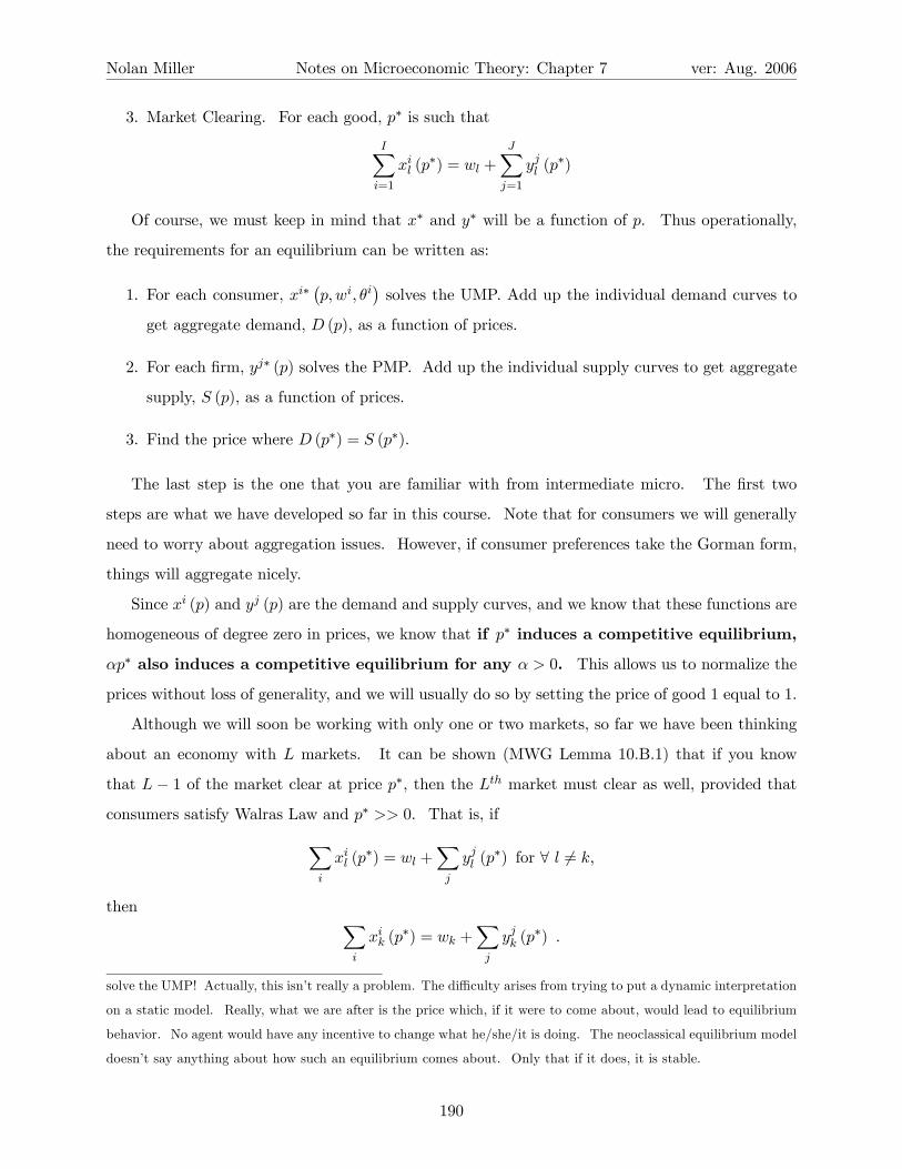
Nolan Miller Notes on Microeconomic Theory: Chapter 7 ver: Aug. 2006
3. Market Clearing. For each good, p∗ is such that
IXi=1
xil (p∗) = wl +
JXj=1
yjl (p∗)
Of course, we must keep in mind that x∗ and y∗ will be a function of p. Thus operationally,
the requirements for an equilibrium can be written as:
1. For each consumer, xi∗¡p,wi, θi
¢solves the UMP. Add up the individual demand curves to
get aggregate demand, D (p), as a function of prices.
2. For each firm, yj∗ (p) solves the PMP. Add up the individual supply curves to get aggregate
supply, S (p), as a function of prices.
3. Find the price where D (p∗) = S (p∗).
The last step is the one that you are familiar with from intermediate micro. The first two
steps are what we have developed so far in this course. Note that for consumers we will generally
need to worry about aggregation issues. However, if consumer preferences take the Gorman form,
things will aggregate nicely.
Since xi (p) and yj (p) are the demand and supply curves, and we know that these functions are
homogeneous of degree zero in prices, we know that if p∗ induces a competitive equilibrium,
αp∗ also induces a competitive equilibrium for any α > 0. This allows us to normalize the
prices without loss of generality, and we will usually do so by setting the price of good 1 equal to 1.
Although we will soon be working with only one or two markets, so far we have been thinking
about an economy with L markets. It can be shown (MWG Lemma 10.B.1) that if you know
that L − 1 of the market clear at price p∗, then the Lth market must clear as well, provided that
consumers satisfy Walras Law and p∗ >> 0. That is, ifXi
xil (p∗) = wl +
Xj
yjl (p∗) for ∀ l 6= k,
then Xi
xik (p∗) = wk +
Xj
yjk (p∗) .
solve the UMP! Actually, this isn’t really a problem. The difficulty arises from trying to put a dynamic interpretation
on a static model. Really, what we are after is the price which, if it were to come about, would lead to equilibrium
behavior. No agent would have any incentive to change what he/she/it is doing. The neoclassical equilibrium model
doesn’t say anything about how such an equilibrium comes about. Only that if it does, it is stable.
190

Nolan Miller Notes on Microeconomic Theory: Chapter 7 ver: Aug. 2006
This lemma is a direct consequence of the idea that total wealth must be preserved in the
economy. The nice thing about it is that when you are only studying two markets, as we do in
the partial equilibrium approach, you know that if one market clears, the other must clear as well.
Hence the study of two markets really reduces to the study of one market.
7.2 Partial Equilibrium Analysis
7.2.1 Set-Up of the Quasilinear Model
We now turn away from the general model to a simple case, known as Partial Equilibrium. It
is ‘partial’ because we focus on a small part of the total economy, often on a two commodity
world. We laid the groundwork for this type of approach in our discussion of consumer theory.
If we are interested in studying a particular market, say the market for apples, we can make the
assumption that the prices of all other commodities move in tandem. This justifies, through use
of the composite commodity theorem, treating consumers as if they have preferences over apples
and “everything else.” Hence we have justified a two-commodity model for this situation. Next,
since each consumer’s expenditure on apples is likely to be only a small part of her total wealth,
it is reasonable to think of there being no wealth effects on consumers’ demand for apples. And,
recall, that quasilinear preferences correspond to the case where there are no wealth effects in the
non-numeraire good. So, basically what we’ll do in our partial equilibrium approach (and what is
implicitly underlying the approach you took in intermediate micro) is assume that there are two
goods: a composite commodity (the numeraire) whose price is set equal to 1, and the good of
interest. We’ll call the numeraire m (for “money”) and the good we are interested in x.
Now, we can set up the following simple model. Let xi and mi be consumer i’s consumption
of the commodity of interest and the numeraire commodity, respectively.3 Assume that each
consumer has quasilinear utility of the form:
ui (mi, xi) = mi + φi (xi) .
Further, we normalize ui (0, 0) = φi (0) = 0, and assume that φ0i > 0 and φ00i < 0 for all xi ≥ 0.
That is, we assume that the consumer’s utility is increasing in the consumption of x and that her
marginal utility of consumption is decreasing.
3This is a change in notation from the set-up at the beginning of the chapter. Now, the subscripts refer to the
consumer / firm, rather than the commodity.
191

Nolan Miller Notes on Microeconomic Theory: Chapter 7 ver: Aug. 2006
Since we already set the price of m equal to 1, we only need to worry about the price of x.
Denote it by p.
There are J firms in the economy. Each firm can transformm into x according to cost function
cj (qj), where qj is the quantity of x that firm j produces, and cj (qj) is the number of units of the
numeraire commodity needed to produce qj units of x. Thus, letting zj denote firm j’s use of good
m as an input, its technology set is therefore
Yj = {(−zj , qj) |qj ≥ 0 and zj ≥ cj (qj)} .
That is, you have to spend enough of good m to produce qj units of x. We will assume that cj (qj)
is strictly increasing and convex for all j.
In order to solve the model, we also need to specify consumers’ initial endowments. We assume
there is no initial endowment of x, but that consumer i has endowment of m equal to wmi > 0 and
the total endowment isP
iwmi = wm.
7.2.2 Analysis of the Quasilinear Model
That completes the set-up of the model. The next step is to analyze it. Recall that in order to find
an equilibrium, we need to derive the firms’ supply functions, the consumers’ demand functions,
and find the market-clearing price.
1. Profit maximization. Given the equilibrium price p∗, firm j’s equilibrium output q∗j must
maximize
maxqj
pqj − cj (qj)
which has the necessary and sufficient first-order condition
p∗ ≤ c0j¡q∗j¢
with equality if q∗j > 0.
2. Utility Maximization: Consumer i’s equilibrium consumption vector (x∗i ,m∗i ) must max-
imize
maxmi + φi (xi)
s.t. mi + p∗xi ≤ wmi +X
θij¡p∗q∗j − cj
¡q∗j¢¢
192

Nolan Miller Notes on Microeconomic Theory: Chapter 7 ver: Aug. 2006
• We know that the budget constraint must hold with equality. We can substitute it into
the objective function for mi, which yields:
maxφi (xi)− p∗xi +hwmi +
Xθij¡p∗q∗j − cj
¡q∗j¢¢i
.
The first-order condition is:
φ0i (x∗i ) ≤ p∗
which holds with equality if x∗i > 0.
3. Market clearing. Remember that lemma that said if one of the markets clears we know
that the other one must clear as well? We will use that to formulate a plan of attack here.
Basically, we will find a price vector such that aggregate demand for x equals aggregate supply
of q,P
i xi (p∗) =
Pj qj (p
∗), i.e. the market for the consumption commodity clears. Then,
we’ll use the budget equation to compute the equilibrium level of mi for each consumer (since
the lemma tells us that the market for the numeraire must clear as well). To begin, assume
an interior solution to the UMP and PMP for each consumer and firm. Then p∗, q∗j , and x∗i
must solve the system of equations
p∗ = c0j (qj (p)) for all j
p∗ = φ0i (xi (p)) for all iXi
xi (p∗) =
Xj
qj (p∗)
Notice that the first j equations determine each firm’s supply function. We can then add
them to get aggregate supply, the RHS of the third equation. The next i equations determine
each consumer’s demand function. We can add them up to get aggregate supply, which is the
LHS of the third equation. The third equation is thus the requirement that at the equilibrium
price supply equals demand.
Notice that the equilibrium conditions involve neither the initial endowments of the consumers
nor their ownership shares. Thus the equilibrium allocation of x and the price of x are independent
of the initial conditions. This follows directly from the assumption of quasilinear utility. However,
since equilibrium allocations of the numeraire are found by using each consumer’s budget constraint,
the equilibrium allocations of the numeraire will depend on initial endowments and ownership
shares.
From a graphical point of view, the partial equilibrium is as follows:
193

Nolan Miller Notes on Microeconomic Theory: Chapter 7 ver: Aug. 2006
1. For each consumer, derive their Walrasian demand for the consumption good, xi (p) . Add
across consumers to derive the aggregate demand, x (p) =P
i xi (p). Since each demand curve
is downward sloping, the aggregate demand curve will be downward sloping. Graphically,
this addition is done by adding the demand curves “horizontally” (as in MWG Figure 10.C.1).
Since individual demand curves are defined by the relation:
p = φ0i (q) ,
The price at which each individual’s demand curve intersects the vertical axis is φ0i (0), and
gives that individual’s marginal willingness to pay for the first unit of output. The intercept
for the aggregate demand curve is therefore maxiφ0i (0). Hence if different consumers have
different φi () functions, not all demand curves will have the same intercept, and the demand
curve will become flatter as price decreases.
2. For each firm, derive the supply curve for the consumption good, yj (p). Add across firms to
derive the aggregate supply, y (p) =P
j yj (p). For each firm, the supply curve is given by:
p = c0j (qj) .
Thus each firm’s supply curve is the inverse of its marginal cost curve. Since we have assumed
that c00j () ≥ 0, the supply curve will be upward sloping or flat. Again, addition is done by
adding the supply curves horizontally, as in MWG Figure 10.C.2. The intercept of the
aggregate supply curve will be the smallest c0j (0). If firms’ cost functions are strictly convex,
aggregate supply will be upward sloping.
3. Find the price where supply equals demand: find p∗ such that x (p∗) = y (p∗). Since the
market clears for good l, it must also clear for the numeraire. The equilibrium point will be
at the price and quantity where the supply and demand curves cross.
At this point, we can talk a bit about the dynamics of how an equilibrium might come about.
This is the story that is frequently told in intermediate micro courses, and I should point out that
it is just a story. There is nothing in the model which justifies this approach since we have said
nothing at all about how markets will behave if they are out of equilibrium. Nevertheless, I’ll tell
the story.
Suppose p∗ is the equilibrium price of x, but that currently the price is equal to p+ > p∗. At
this price, aggregate demand is less than aggregate supply: D (p∗) < S (p∗) . Because of this, there
194
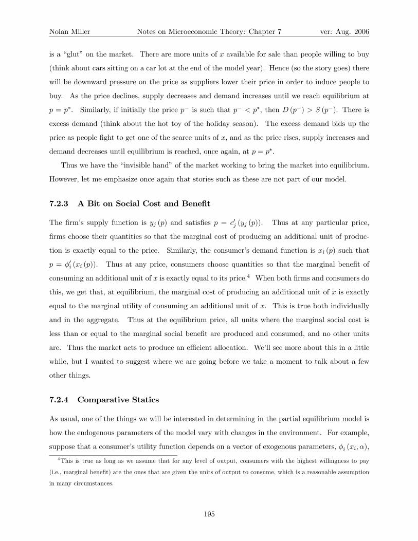
Nolan Miller Notes on Microeconomic Theory: Chapter 7 ver: Aug. 2006
is a “glut” on the market. There are more units of x available for sale than people willing to buy
(think about cars sitting on a car lot at the end of the model year). Hence (so the story goes) there
will be downward pressure on the price as suppliers lower their price in order to induce people to
buy. As the price declines, supply decreases and demand increases until we reach equilibrium at
p = p∗. Similarly, if initially the price p− is such that p− < p∗, then D (p−) > S (p−). There is
excess demand (think about the hot toy of the holiday season). The excess demand bids up the
price as people fight to get one of the scarce units of x, and as the price rises, supply increases and
demand decreases until equilibrium is reached, once again, at p = p∗.
Thus we have the “invisible hand” of the market working to bring the market into equilibrium.
However, let me emphasize once again that stories such as these are not part of our model.
7.2.3 A Bit on Social Cost and Benefit
The firm’s supply function is yj (p) and satisfies p = c0j (yj (p)). Thus at any particular price,
firms choose their quantities so that the marginal cost of producing an additional unit of produc-
tion is exactly equal to the price. Similarly, the consumer’s demand function is xi (p) such that
p = φ0i (xi (p)). Thus at any price, consumers choose quantities so that the marginal benefit of
consuming an additional unit of x is exactly equal to its price.4 When both firms and consumers do
this, we get that, at equilibrium, the marginal cost of producing an additional unit of x is exactly
equal to the marginal utility of consuming an additional unit of x. This is true both individually
and in the aggregate. Thus at the equilibrium price, all units where the marginal social cost is
less than or equal to the marginal social benefit are produced and consumed, and no other units
are. Thus the market acts to produce an efficient allocation. We’ll see more about this in a little
while, but I wanted to suggest where we are going before we take a moment to talk about a few
other things.
7.2.4 Comparative Statics
As usual, one of the things we will be interested in determining in the partial equilibrium model is
how the endogenous parameters of the model vary with changes in the environment. For example,
suppose that a consumer’s utility function depends on a vector of exogenous parameters, φi (xi, α),
4This is true as long as we assume that for any level of output, consumers with the highest willingness to pay
(i.e., marginal benefit) are the ones that are given the units of output to consume, which is a reasonable assumption
in many circumstances.
195

Nolan Miller Notes on Microeconomic Theory: Chapter 7 ver: Aug. 2006
P
q, x
S
D
DWL
pc
pf
t
Qt Q*
Figure 7.2: Partial Equilibrium with a Tax
and a firm’s cost function depends on another vector of parameters (possibly overlapping), cj (qj , β) .
Note that α and β will include at least the prices of the commodities, but may include other things
such as tax rates, taste parameters, etc. We can ask how the equilibrium prices and quantities
change with a change in α or β.
One of the most studied situations of this type is the impact of a tax on good x. Suppose,
for example, that the government collects a tax of t on each unit of output purchased. Let the
price consumers pay be pc and the price producers receive be pf . Note that consumers only care
about the price they have to pay to acquire the good, and producers only care about the price they
receive when the sell a unit of the good. In particular, neither side of the market cares directly
about the tax. The two prices are related by the tax rate:
pc = pf + t.
The equilibrium in this market is the point where supply equals demand, i.e., prices pc and pf
such that
x (pc) = q (pf ) , and
pc = pf + t.
Or,
x (pf + t) = q (pf ) .
The equilibrium is depicted in Figure 7.2:
196

Nolan Miller Notes on Microeconomic Theory: Chapter 7 ver: Aug. 2006
Qt is the quantity sold after the tax is implemented. At this quantity, the difference between
the price paid by consumers and the price received by firms is exactly equal to the tax. Note
that at Qt, the marginal social cost of an additional unit of output is less than the marginal social
benefit. Hence society could be made better off if additional units of output were produced and
sold, all the way up to the point where Q∗ units of output are produced. The loss suffered by
society due to the fact that these units are not produced and consumed is called the deadweight
loss (DWL) of taxation.
One question we may be interested in is how the price paid by consumers changes when the size
of the tax increases. Let p∗ (t) be the equilibrium price received by firms. Thus consumers pay
p∗ (t) + t. The following identity holds for any tax rate t :
x (p∗ (t) + t) ≡ q (p∗ (t)) .
Totally differentiating with respect to t yields:
x0 (p∗ + t)¡p0 (t) + 1
¢= q0 (p∗) p0 (t)
p0 (t) =−x0 (p∗ + t)
x0 (p∗ + t)− q0 (p∗)
The numerator is positive by definition. Since q0 (p∗) is positive, the absolute value of the denom-
inator is larger than the absolute value of the numerator, hence −1 < p0 (t) < 0. This implies that
as the tax rate increases, the price received by firms decreases, but by less than the full amount of
the tax. As a consequence, the price paid by consumers must also increase, but by less than the
increase in the tax. Further, the total quantity must decrease as well.
Consider the formula we just derived:
p0 (t) =−x0 (p∗ + t)
x0 (p∗ + t)− q0 (p∗).
Evaluate at t = 0, and rewrite this in terms of elasticities:
dp
dt=
−dxdp
px
dxdp
px −
dqdp
pq
= − |εd||εd|+ εs
where εd is the elasticity of demand and εs is the elasticity of supply. This says that the proportion
of a small tax that is passed onto producers in the form of lower prices is given by |εd||εd|+εs . The
proportion passed onto consumers in the form of higher prices is given by εs|εd|+εs .
197

Nolan Miller Notes on Microeconomic Theory: Chapter 7 ver: Aug. 2006
Now, suppose the government is considering two different tax programs: one that taxes a
commodity with relatively inelastic demand, and one that taxes a commodity with relatively elastic
demand. Which will result in the larger deadweight loss? The answer is, all else being equal, the
commodity with the more elastic demand will have a larger deadweight loss. Why? The more
elastic demand is, the flatter the demand curve will be. This means that a more elastic demand
curve will respond to a tax with a relatively larger decrease in quantity. And, since this quantity
distortion is the source of the deadweight loss, the more elastic demand curve will result in the
larger deadweight loss.
Does this mean that we should only tax inelastic things, since this will make society better off?
Not really. The main reason is that even though taxing inelastic things may be better for society as
a whole from an efficiency standpoint, it may have undesirable redistributive effects. For example,
we could tax cigarette smokers and force them to pay for road construction and schools. Since
cigarette demand is relatively inelastic, this would result in a relatively small deadweight loss.
However, is it really fair to force smokers to pay for roads and schools, even though they don’t
necessarily use the roads and schools any more intensely than other people? Probably not. We
recently had a related issue in Massachusetts. The state wanted to increase tolls on the turnpike
in order to pay for construction at the airport. Turnpike usage is relatively inelastic, but is it fair
to make turnpike users pay for airport construction, even though turnpike users are no more likely
to be going to the airport than other drivers? Issues of balancing efficiency and equity concerns
such as this arise often in policy decisions.
7.3 The Fundamental Welfare Theorems
Recall that we ended our discussion of production by talking about efficiency, and showed that
any profit-maximizing production plan is efficient (i.e. the same output cannot be produced using
fewer inputs), and that any efficient production plan (under certain circumstances) is the profit
maximizing production plan for some price vector. We now turn to ask the same questions of
markets. That is, when are the allocations made by markets “efficient,” and is every efficient
allocation the market allocation for some initial conditions? Again, the reason we ask these
questions has to do with decentralization. When can we decentralize the decisions we make in our
society? Do we know that profit-maximizing firms and utility maximizing agents will arrive at a
Pareto optimal allocation through the market? If we have a particular Pareto optimal allocation
198

Nolan Miller Notes on Microeconomic Theory: Chapter 7 ver: Aug. 2006
in mind, can we rely on the market to get us there, provided we start at the right place (i.e., initial
endowment for consumers)?
The proper concept of efficiency here is Pareto optimality. Recall that an allocation is Pareto
optimal if there is no other feasible allocation that makes all agents at least as well off and some
agent better off. We will study Pareto optimal allocations in the context of the quasilinear partial
equilibrium model we introduced earlier. This greatly simplifies the analysis, since when preferences
are quasilinear, the frontier of the utility possibility set is linear. That is, all points that are Pareto
efficient involve the same consumption of the non-numeraire good by the consumers, and differ only
in the distribution of the numeraire among the consumers.
To illustrate this point, suppose there are two consumers, and fix the consumption and produc-
tion levels at x and q respectively. This will leave wm−P
j cj (qj) of the numeraire to be distributed
among the consumers. Since the numeraire can be traded one-for-one among consumers, the utility
possibility set for this x∗ and q∗ is the set⎧⎨⎩(u1, u2) |u1 + u2 ≤ φ1 (x1) + φ2 (x2) + wm −Xj
cj (qj)
⎫⎬⎭This is the utility possibility set for any particular allocation of the consumption good, (x, q),
if we allow the remaining numeraire to be distributed among consumers in any possible way. The
utility possibility set for the efficient allocation is the set generated by the x∗1 and x∗2 that maximize
the right hand side of this expression: That is, Pareto optimal allocations satisfy:
x∗1, x∗2, q
∗j ∈ argmaxφ1 (x1) + φ2 (x2) + wm −
Xj
cj (qj)
subject to : x1 + x2 =X
qj
We will call the x’s and q’s generated by such a procedure the optimal production and consump-
tion levels of good x. If the firms have strictly concave production functions and φi () is strictly
concave, then there will be a unique (x, q) that maximizes the above expression.
We can rewrite the above problem in the multiple consumer case as:
maxx,q
ÃXi
φi (xi)
!+ wm −
⎛⎝Xj
cj (qj)
⎞⎠subject to :
IXi=1
xi −JX
j=1
qj = 0
199

Nolan Miller Notes on Microeconomic Theory: Chapter 7 ver: Aug. 2006
The top line just says to maximize the sum of the consumers’ utilities. The constraint is that
the total consumption of x is the same as the total production. Letting the Lagrange multiplier
be μ, the first-order conditions for this problem are:
φ0i (x∗i ) ≤ μ with equality if x∗i > 0
c0j¡q∗j¢≥ μ with equality if q∗j > 0
IXi=1
x∗i =JX
j=1
q∗j
Note that these are exactly the conditions as the conditions defining the competitive equilibrium
except that p∗ has been replaced by μ. In other words, we know that the allocation produced by
the competitive market satisfies these conditions, and that μ = p∗. Thus the competitive market
allocation is Pareto optimal, and the market clearing price p∗ is the shadow value of the constraint:
the additional social benefit generated by consuming one more unit of output or producing one less
unit of output. Hence this is just another expression of the fact that at p∗ the marginal social
benefit of additional output equals the marginal social cost.
The preceding argument establishes the first fundamental theorem of welfare economics
in the partial equilibrium case. If the price p∗ and the allocation (x∗, q∗) constitute a competitive
equilibrium, then this allocation is Pareto optimal.
The first theorem is just a formal expression of Adam Smith’s invisible hand — the market acts
to allocate commodities in a Pareto optimal manner. Since p∗ = μ, which is the shadow price
of additional units of x, each firm acting in order to maximize its own profits chooses the output
that equates the marginal cost of its production to the marginal social benefit, and each consumer,
in choosing the quantity to consume in order to maximize utility, is also setting marginal benefit
equal to the marginal social cost.
Note that while this is a special case, the first welfare theorem will hold quite generally whenever
there are complete markets, no matter how many commodities there are. It will fail, however,
when there are commodities (things that affect utility) that have no markets (as in the externalities
problem we’ll look at soon).
As we did with production, we can also look at this problem “backward.” Can any Pareto
optimal allocation be generated as the outcome of a competitive market, for some suitable initial
endowment vector? The answer to this question is yes.
To see why, recall that when all φi ()’s are strictly concave and all cj ()’s are strictly convex, there
is a unique allocation of the consumption commodity x that maximizes the sum of the consumers’
200

Nolan Miller Notes on Microeconomic Theory: Chapter 7 ver: Aug. 2006
utilities. The set of Pareto optimal allocations is derived by allocating the consumption commodity
in this manner and varying the amount of the numeraire commodity given to each of the consumers.
Thus the set of Pareto optimal allocations is a line with normal vector (1,1,1...,1) (see, for example,
Figure 10.D.1 in MWG), since one unit of utility can be transferred from one consumer to another
by transferring a unit of the numeraire.
Thus any Pareto optimal allocation can be generated by letting the market work and then ap-
propriately transferring the numeraire. But, recall that firms’ production decisions and consumers’
consumption decisions do not depend on the initial endowment of the numeraire. Because of this,
we could also perform these transfers before the market works. This allows us to implement any
point along the Pareto frontier.
To see why, let (x∗, q∗) be the Pareto optimal allocation of the consumption commodity, and
suppose we want to implement the point where each consumer gets (x∗i ,m∗i ) after the market works,
whereP
im∗i = wm −
Pj cj
³q∗j
´. If we want consumer i to have m∗i units of the numeraire after
the transfer, we need him to have m0i before the transfer, where
m0i +
Xθij¡p∗q∗j − cj
¡q∗j¢¢= m∗i + p∗x∗i .
Hence if people have wealth m0i before the market starts to work, allocation (x
∗, q∗,m∗) will result.
This yields the second fundamental theorem of welfare economics. Let u∗i be the utility in a
Pareto optimal allocation for some initial endowment vector. There exists a set of transfers Ti (the
amount of the numeraire given to consumer i) such thatP
i Ti = 0 and the allocation generated by
the competitive market yields the utility vector u∗.
The transfers are given by Ti = m0i − wmi.
7.3.1 Welfare Analysis and Partial Equilibrium
Recall in our discussion of consumer theory we said that equivalent variation is the proper measure
of the impact of a policy change on consumers, and that EV is given by the area to the left of the
Hicksian demand curve between the initial and final prices. However, since there are no wealth
effects for the consumption good here, we know that the Hicksian and Walrasian demand curves are
the same. So, the area to the left of the Walrasian demand curve is a proper measure of consumer
welfare. Further, since utility is quasilinear, it makes sense to look at aggregate demand, and there
is a normative representative consumer whose preferences are captured by the aggregate demand
curve. Hence the area to the left of the Walrasian demand curve is a good measure of changes in
201

Nolan Miller Notes on Microeconomic Theory: Chapter 7 ver: Aug. 2006
social welfare.
It is worthwhile to derive a measure of aggregate social surplus here, even though we already
did it during our study of aggregation. Recall the Pareto optimality problem:5
maxx,q
ÃXi
φi (xi)
!+ wm −
⎛⎝Xj
cj (qj)
⎞⎠subject to :
IXi=1
xi −JX
j=1
qj = 0.
We said that the solution to this problem determines the allocation that maximizes consumers’
welfare (and therefore societal welfare).
Consider the objective function:ÃXi
φi (xi)
!−
⎛⎝Xj
cj (qj)
⎞⎠+wm.
The last term is the initial aggregate endowment of the numeraire good, which is just a constant
in the objective function. The first two terms represent the difference between aggregate utility
from consumption and aggregate cost of production. It is this difference that we are maximizing
in the Pareto optimality problem.
Consider a single unit of production. The difference between the utility derived from that
production and the cost of production is the societal benefit from that good (since all profits return
to consumers). If we add this surplus across all consumers, that gets usÃXi
φi (xi)
!−
⎛⎝Xj
cj (qj)
⎞⎠which is the surplus generated by all units of production. This term, called Marshallian Aggregate
Surplus (MAS), is the measure of social benefit that we want to use, since it tells us how much
better off society is made whenP
i xi =P
j qj units of the non-numeraire good are produced and
sold.
To better understand, note that we can break the surplus down into four parts:
1. (a) Some of the surplus comes from consumption,P
i φi (xi),
(b) Some surplus is lost due to paying price p for the good.
•P
i φi (xi)− pxi is the aggregate consumer surplus
5This corresponds to the utilitarian social welfare problem.
202
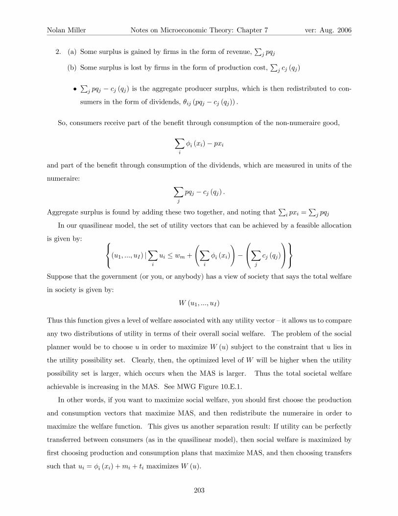
Nolan Miller Notes on Microeconomic Theory: Chapter 7 ver: Aug. 2006
2. (a) Some surplus is gained by firms in the form of revenue,P
j pqj
(b) Some surplus is lost by firms in the form of production cost,P
j cj (qj)
•P
j pqj − cj (qj) is the aggregate producer surplus, which is then redistributed to con-
sumers in the form of dividends, θij (pqj − cj (qj)) .
So, consumers receive part of the benefit through consumption of the non-numeraire good,
Xi
φi (xi)− pxi
and part of the benefit through consumption of the dividends, which are measured in units of the
numeraire: Xj
pqj − cj (qj) .
Aggregate surplus is found by adding these two together, and noting thatP
i pxi =P
j pqj
In our quasilinear model, the set of utility vectors that can be achieved by a feasible allocation
is given by: ⎧⎨⎩(u1, ..., uI) |Xi
ui ≤ wm +
ÃXi
φi (xi)
!−
⎛⎝Xj
cj (qj)
⎞⎠⎫⎬⎭Suppose that the government (or you, or anybody) has a view of society that says the total welfare
in society is given by:
W (u1, ..., uI)
Thus this function gives a level of welfare associated with any utility vector — it allows us to compare
any two distributions of utility in terms of their overall social welfare. The problem of the social
planner would be to choose u in order to maximize W (u) subject to the constraint that u lies in
the utility possibility set. Clearly, then, the optimized level of W will be higher when the utility
possibility set is larger, which occurs when the MAS is larger. Thus the total societal welfare
achievable is increasing in the MAS. See MWG Figure 10.E.1.
In other words, if you want to maximize social welfare, you should first choose the production
and consumption vectors that maximize MAS, and then redistribute the numeraire in order to
maximize the welfare function. This gives us another separation result: If utility can be perfectly
transferred between consumers (as in the quasilinear model), then social welfare is maximized by
first choosing production and consumption plans that maximize MAS, and then choosing transfers
such that ui = φi (xi) +mi + ti maximizes W (u).
203
Nolan Miller Notes on Microeconomic Theory: Chapter 7 ver: Aug. 2006
Now, how does MAS change when the quantity produced and consumed changes? Let S (x, q)
be the MAS, formally defined as follows:
S (x, q) =
ÃXi
φi (xi)
!−
⎛⎝Xj
cj (qj)
⎞⎠ .
Consider a differential increase in consumption and production: (dx1, dx2, ..., dxI , dq1, ...dqJ) sat-
isfyingP
i dxi =P
j dqj . Note that under such a change, we increase total production and total
consumption by the same amount.
The differential in S is given by
dS =
ÃXi
φ0i (xi) dxi
!−
⎛⎝Xj
c0j (qj) dqj
⎞⎠ .
Since consumers maximize utility, φ0i (xi) = p (x) for all i, and since producers maximize profit,
c0j (qj) = c0 (q) for all j. Thus:
dS =
Ãp (x)
Xi
dxi
!−
⎛⎝c0 (q)Xj
dqj
⎞⎠which by definition of our changes (and market clearing) implies
dS =¡p (x)− c0 (q)
¢dx
And, integrating this from 0 to x yields that MAS equals
S (x) =
Z x
0
¡p (s)− c0 (s)
¢ds.
Thus the total surplus is the area between the supply and demand curves between 0 and the
quantity sold, x.
Example: Welfare Effects of a Tax
We return to the idea of a commodity tax that we first considered in the context of consumer
theory. Suppose there is a government that attempts to maximize the welfare of its citizens. The
government keeps a balanced budget, and tax revenues are returned to consumers in the form of a
lump sum transfer.
What are the welfare effects of this tax? Define x∗1 (t) , ..., x∗I (t) and q∗1 (t) , ..., q
∗J (t) and p∗ (t),
respectively, to be the consumptions, productions, and price paid by consumers when the per-unit
204

Nolan Miller Notes on Microeconomic Theory: Chapter 7 ver: Aug. 2006
tax is t. Define x∗ (t) =P
x∗i (t) and q∗ (t) =
Pq∗j (t) to be aggregate consumption and production,
respectively. Letting S∗ (t) =P
x∗i (t)−P
q∗j (t) be the level of MAS (also equal to the area below
the demand curve and above the supply curve) at tax rate t, the change in MAS when a tax of t
is imposed is given by:
S∗ (x∗ (t))− S∗ (x∗ (0)) = x∗ (t)− q∗ (t)− (x∗ (0)− q∗ (0))
=
Z x∗(t)
x∗(0)p(s)− c0 (s) ds,
by the definition of MAS developed earlier. Thus the change in MAS is given by the change in
the area between the aggregate demand and supply curves, between the equilibrium quantity when
there is no tax and the equilibrium quantity after the tax is imposed. Note that this is just the
area we called deadweight loss earlier.
7.4 Entry and Long-Run Competitive Equilibrium
Up until now, we have considered the competitive equilibrium holding the supply side of the market
fixed. In particular, we have assumed:
1. Firms are unable to vary their fixed factors of production (plant size is fixed)
2. Firms are unable to enter or exit the market — the number of firms stay fixed
These assumptions are appropriate in the short run. However, if we want to examine the
behavior of the market in the long run, we must explicitly allow for firms to change their fixed
factors, including entering or exiting the industry.
In the long run, a perfectly competitive market is characterized by:
1. Firms and consumers are price takers
2. Free entry and exit
The free entry and exit condition doesn’t mean that firms can enter at no cost. Rather, it
means that there is no impediment to them incurring the cost and entering the market. For
example, there are no laws against entry, there are no proprietary technologies or scarce resources,
etc. Thus firms have the freedom to enter or exit, but this is not to say that they can do it for
free. In our discussion up until now, we have considered only the price-taking requirement. In
order to think about competitive equilibrium in the long run, we add the free entry condition.
205
Nolan Miller Notes on Microeconomic Theory: Chapter 7 ver: Aug. 2006
S
D
P
Q
$
Q
profit
MC AC
qi*
Q*
P*
Figure 7.3: Short-Run Equilibrium
7.4.1 Long-Run Competitive Equilibrium
Consider our analysis of perfect equilibrium in the short run.6 The short-run equilibrium price
and quantity are found where supply equals demand for a given number of firms. However, note
that if there happen to be a small number of firms in an industry, it may be that the firms are
making large profits.
Figure 7.3 links the market equilibrium with the individual firm. On the left, aggregate supply
and demand combine to determine the equilibrium price, P ∗. At this price, the individual firm’s
behavior is depicted in the right panel. The firm chooses to produce q∗i units of output, and earns
q∗i (P∗ −AC (q∗i )) profit. Total profit by the firm is shaded in the right-hand panel.
Now, if you are a business person, you see an industry where firms are making large profits,
and you can enter it if you want, what do you do? You enter. When you enter, what happens to
the supply curve? It shifts out to the right. And, as the supply curve shifts right, the equilibrium
price decreases, which decreases the profit of the firms already in the industry.
How many firms enter? As long as a firm can earn a positive profit by entering the industry,
it will choose to enter. Thus firms will continue to enter until they drive profit to zero. This
situation is shown in Figure 7.4.
Note that profit equals zero when the equilibrium price, denoted by P 0 in the diagram, is such
6 Implicit in the arguments for this section is the idea that all firms, both those that are in the market and those
who could potentially enter the market, have the same technology. The conclusions can be adapted to the case where
technologies are heterogeneous without changing the results too much.
206

Nolan Miller Notes on Microeconomic Theory: Chapter 7 ver: Aug. 2006
S
D
P
Q
$
Q
MC AC
qi'
Q’
S’
P’
Figure 7.4: Long-Run Equilibrium
that P 0 = minAC.
Similarly, if there are initially too many firms in the industry, the firms in the industry will earn
negative profits. This will drive firms to exit the industry. As they exit the industry, the price
will increase, and the size of the firms’ losses will decrease. When does exit stop? When the firms
that are in the industry earn zero profit. You should draw the diagram for this case.
The dynamic story I’ve been telling suggests the following requirements for a long-run compet-
itive equilibrium. First, we keep the requirements for a short-run equilibrium:
1. (a) Firms maximize profits
(b) Consumers maximize utility
(c) Market clearing: price adjusts so that supply equals demand
Second, we add the additional requirement that the equilibrium number of firms is found where
in the short-run equilibrium firms make zero profit.7
Formally, if there are a very large number of identical firms that could potentially enter this
market, this means that the equilibrium consists of q∗, p∗, J∗ that satisfy:
1. q∗ maximizes p∗q − c (q) for each firm.
2. x∗i maximizes ui (xi)− pxi for all i
7There is something of an integer problem here. That is, it may be if there are J∗ firms all firms earn a positive
profit, but if there are J∗ + 1 firms, all firms earn a negative profit. In this case, we will say that the equilibrium is
the largest number of firms such that firms do not earn negative profits.
207

Nolan Miller Notes on Microeconomic Theory: Chapter 7 ver: Aug. 2006
3. x (p∗) = J∗q∗ : market clearing
4. p∗q∗ − c (q∗) = 0 : free entry
The last requirement is one way to think of the free entry condition. Entry continues until all
firms make zero profit. Another way to think of it is as follows: Entry will continue until the
point that with J∗ firms in the industry, all firms make non-negative profits. With J∗+1 firms in
the industry, all firms make negative profits. Thus it need not be the case that all firms make zero
profits. But, it must be the case that if one more firm enters, all firms will make negative profits.
Thus J∗ is the maximum number of firms that can be supported by this market.
What will the long-run aggregate supply correspondence look like? Since all firms are the same,
the long-run aggregate supply correspondence as a function of p will look as follows:
Q (p) = ∞ if π (p) > 0
= Jq for some integer J ≥ 0 and q ∈ q (p) if π (p) = 0
= 0 if π (p) < 0
That is, if the price is such that profits are positive, an infinite number of firms will enter the
industry — driving the quantity supplied to infinity. If price is such that profits are zero then some
integer number of firms will enter the market and produce q according to its supply function q (p).
When profits are negative at a specific price, firms will supply nothing. Generally, however, we
won’t worry about the integer problems here. We’ll assume that in the long run, the supply curve
is horizontal at the level of minimum average cost.
Example: Consider the case of constant returns to scale technology with no fixed cost:
c (q) = cq.
• In this case, firms will supply an infinite amount when p > c, any positive amount when
p = c, and zero when p < c.
• The long-run equilibrium will be where demand and long-run supply cross, which is at p = c.
However, we don’t know how many firms there will be, since the firms could split up the
quantity they want to produce in any way they want. It is a long-run equilibrium with any
number of firms!
208
Nolan Miller Notes on Microeconomic Theory: Chapter 7 ver: Aug. 2006
Example: Firms have strictly increasing, strictly convex cost
• In this case, firms make a positive profit whenever p > c0 (0). Hence entry will continue,
driving price down until it reaches c0 (0) , and all firms make zero profit.
• This makes sense — convex cost is the same as decreasing returns to scale. In this case, the
most efficient firms are those that are producing no output at all. So, as price decreases,
firms are driven to produce more efficiently, and that involves producing lower quantities.
Example: Firms Have U-Shaped Cost Curves
Now suppose that the firm has a cost function that is first concave, and then convex, giving a
U-shaped average cost curve. In the long run, price will be driven down to the point where
p = minAC. In that case, each firm will produce the quantity that minimizes AC. Thus the
long-run aggregate supply function is given by:
Q (p) = ∞ if p > minAC
= Jq if p = minAC, where q = q(minAC)
= 0 if p < minAC
Note that it is possible that when p = minAC, there is no J such that J · q (minAC) =
x (minAC). This is known as the integer problem. There are several reasons to think that the
integer problem is not such a horrible thing:
• If firms are small relative to the market, then there will be a J such that J · q (minAC) is
close to x (minAC)
• Long-run equilibrium is a theoretical construct — we never really get there, but we’re always
moving toward there.
• If the price is slightly above minAC, then the supply curve will be upward sloping. Thus
we are really looking for the largest J such that p > minAC. These firms will make a slight
profit.
7.4.2 Final Comments on Partial Equilibrium
The approach to partial equilibrium we have adopted has been based on a quasilinear model. How
crucial is this for the results? Well, the quasilinear utility is not critical for the determination of
209

Nolan Miller Notes on Microeconomic Theory: Chapter 7 ver: Aug. 2006
the competitive equilibrium — you would still find it in the same way. However, it is critical for the
welfare results. Without quasilinear utility, the area under the Walrasian demand curves doesn’t
mean anything — so we will need a different welfare measure. Further, with wealth effects, welfare
will depend on the distribution of the numeraire, not just the consumption good, which means that
we will have to do additional work.
210

Chapter 8
Externalities and Public Goods
8.1 What is an Externality?
We just showed that competitive markets result in Pareto optimal allocations — that is the market
acts to make sure that those who value goods the most receive them, and those that can produce
goods at the least cost produce them, and there is no way that everybody in society could be made
better off. This gave us the first and second welfare theorems — the market allocates commodities
efficiently, and any efficient allocation can be derived by a market with suitable ex ante transfers
of wealth. Now we will take a look at one important circumstance where the welfare theorems do
not hold.
When we talked about commodities in the past, they were always what are called “private
goods.” That is, they were such that they were consumed by only one person, and that person’s
consumption of the good had no effect on other people’s utility. But, this is not true of all goods.
Think, for example, of a local bakery that produces bread. Earlier, we said that each person
purchases the quantity of bread where the marginal benefit of consuming an additional loaf is just
equal to the price of a loaf, and each firm produces bread up to the point where the marginal cost
of producing the loaf is just equal to its price. In equilibrium, then, the marginal benefit of eating
an additional loaf of bread is just equal to the marginal cost of producing an additional loaf. But,
think about the following. People who walk by the bakery get the benefit from the pleasant smell
of baking bread, and this is not incorporated into the price of bread. Thus at the equilibrium, the
marginal social benefit of another loaf of bread is equal to the benefit people get from eating the
bread as well as the benefit people get from the pleasant smell of baking bread. However, since
bread purchasers do not take into account the benefit provided to people who do not purchase
211
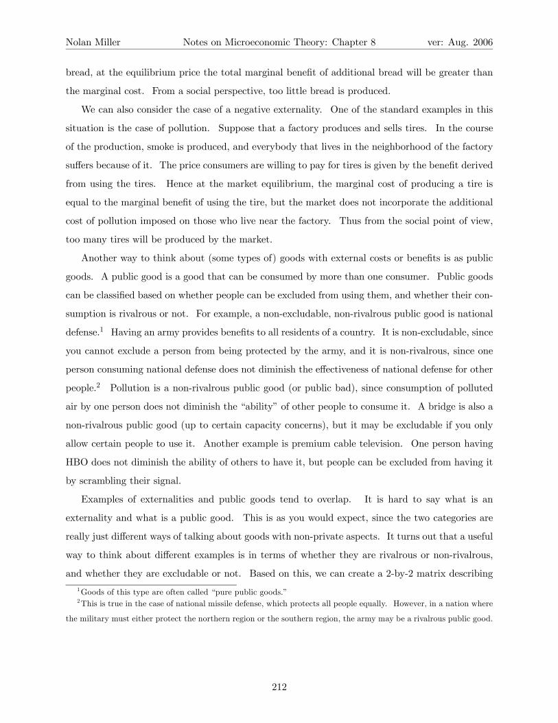
Nolan Miller Notes on Microeconomic Theory: Chapter 8 ver: Aug. 2006
bread, at the equilibrium price the total marginal benefit of additional bread will be greater than
the marginal cost. From a social perspective, too little bread is produced.
We can also consider the case of a negative externality. One of the standard examples in this
situation is the case of pollution. Suppose that a factory produces and sells tires. In the course
of the production, smoke is produced, and everybody that lives in the neighborhood of the factory
suffers because of it. The price consumers are willing to pay for tires is given by the benefit derived
from using the tires. Hence at the market equilibrium, the marginal cost of producing a tire is
equal to the marginal benefit of using the tire, but the market does not incorporate the additional
cost of pollution imposed on those who live near the factory. Thus from the social point of view,
too many tires will be produced by the market.
Another way to think about (some types of) goods with external costs or benefits is as public
goods. A public good is a good that can be consumed by more than one consumer. Public goods
can be classified based on whether people can be excluded from using them, and whether their con-
sumption is rivalrous or not. For example, a non-excludable, non-rivalrous public good is national
defense.1 Having an army provides benefits to all residents of a country. It is non-excludable, since
you cannot exclude a person from being protected by the army, and it is non-rivalrous, since one
person consuming national defense does not diminish the effectiveness of national defense for other
people.2 Pollution is a non-rivalrous public good (or public bad), since consumption of polluted
air by one person does not diminish the “ability” of other people to consume it. A bridge is also a
non-rivalrous public good (up to certain capacity concerns), but it may be excludable if you only
allow certain people to use it. Another example is premium cable television. One person having
HBO does not diminish the ability of others to have it, but people can be excluded from having it
by scrambling their signal.
Examples of externalities and public goods tend to overlap. It is hard to say what is an
externality and what is a public good. This is as you would expect, since the two categories are
really just different ways of talking about goods with non-private aspects. It turns out that a useful
way to think about different examples is in terms of whether they are rivalrous or non-rivalrous,
and whether they are excludable or not. Based on this, we can create a 2-by-2 matrix describing
1Goods of this type are often called “pure public goods.”2This is true in the case of national missile defense, which protects all people equally. However, in a nation where
the military must either protect the northern region or the southern region, the army may be a rivalrous public good.
212

Nolan Miller Notes on Microeconomic Theory: Chapter 8 ver: Aug. 2006
goods.3
Non-rivalrous Rivalrous
Non-Excludable (Pure) Public Goods Common-Pool Resources
Excludable Club Goods Private Goods
Private goods are goods where consumption by one person prevents consumption by another
(an extreme form of rivalrous consumption), and one person has the right to prevent the other
from consuming the object. When consumption is non-rivalrous but excludable, as in the case
of a bridge, such goods are sometimes called club goods. Because club goods are excludable,
inefficiencies due to external effects can often be addressed by charging people for access to the
club goods, such as charging a toll for a bridge or a membership fee for a club. Pure public
goods are goods such as national defense, where consumption is non-rivalrous and non-excludable.
Common-pool resources are goods such as national fisheries or forests, where consumption is
rivalrous but it is difficult to exclude people from consuming them. Both pure public goods and
common-pool resources are situations where the market will fail to allocate resources efficiently.
After considering a simple, bilateral externality, we will go on to study pure public goods and
common pool resources in greater detail.
8.2 Bilateral Externalities
We begin with the following definition. An externality is present whenever the well-being of a
consumer or the production possibilities of a firm are directly affected by the actions of another
agent in the economy (and this interaction is not mediated by the price mechanism). An important
feature of this definition is the word “directly.” This is because we want to differentiate between a
true externality, and what is called a pecuniary externality. For example, return to the example
of the bakery we considered earlier. We can think of three kinds of external effects. First, there
is the fact, as we discussed earlier, that consumers walking down the street may get utility from
the smell of baking bread. This is true regardless of whether the people participate in any market.
Second, if the smells of the bread are pleasant enough, the bakery may be able to charge more
for the bread it sells, and, the fact that the price of bread increases may have harmful effects on
people who buy the bread because they must pay more for the bread. We call this type of effect
a pecuniary externality, since it works through the price mechanism. Effects such as this are not
3Based on Ostrom, Rules, Games, and Common Pool Resources, University of Michigan Press, 1994.
213

Nolan Miller Notes on Microeconomic Theory: Chapter 8 ver: Aug. 2006
really externalities, and will not have the distortionary effects we will find with true externalities.4
Third, there is the fact that being next to a bakery may increase rents in the area around it. While
this is a situation where the bakery has effects outside of the bread market, this effect is captured
by the rent paid by other stores in the area. Whether this is an externality or not depends on the
particular situation. For example, if you own an apartment building next to the bakery before it
opens and are able to increase rents after it begins to produce bread, they you have realized an
external benefit from the bakery (since the bakery has increased the value of your property). On
the other hand, if you purchase the building next to the bakery once it is already opened, then you
will pay a higher price for the building, but this is the fair price for a building next to a bakery.
Thus this situation is really more of a pecuniary externality than a true externality.
We will use the following example for our externality model. There are two consumers, i = 1, 2.
There are L traded goods in the economy with price vector p, and the actions taken by these two
consumers do not affect the prices of these goods. That is, the consumers are price takers. Further,
consumer i has initial wealth wi.
Each consumer has preferences over both the commodities he consumes and over some action
h that is taken by consumer 1. That is,
ui¡xi1, ..., x
iL, h
¢.
Activity h is something that has no direct monetary cost for person 1. For example, it could be
playing loud music. Loud music itself has no cost. In order to play it, the consumer must purchase
electricity, but electricity can be captured as one of the components of xi.
From the point of view of consumer 2, h represents an external effect of consumer 1’s action.
In the model, we assume that∂u2∂h
6= 0.
Thus the externality in this model lies in the fact that h affects consumer 2’s utility, but it is not
priced by the market. For example, h is the quantity of loud music played by person 1.
Let vi (p,wi, h) be consumer i’s indirect utility function:
vi (wi, h) = maxxi
ui (xi, h)
s.t. p · xi ≤ wi.
4The key to being a true externality is that the external effect will usually be on parties that are not participants
in the market we are studying, in this case the market for bread.
214

Nolan Miller Notes on Microeconomic Theory: Chapter 8 ver: Aug. 2006
We will also make the additional assumption that preferences are quasilinear with respect to some
numeraire commodity. If this were not so, then the optimal level of the externality would depend
on the consumer’s level of wealth, significantly complicating the analysis.
When preferences are quasilinear, the consumer’s indirect utility function takes the form:
vi (wi, h) = φi (h) + wi.5
Since we are going to be concerned with the behavior of utility with respect to h but not p, we will
suppress the price argument in the utility function. That is, let φi (h) = φi (p, h), when we hold
the price p constant. We will assume that utility is concave in h : φ00i (h) < 0.
Now, we want to derive the competitive equilibrium outcome, and show that it is not Pareto
optimal. How will consumer 1 choose h? The function v1 gives the highest utility the consumer
can achieve for any level of h. Thus in order to maximize utility, the consumer should choose h in
order to maximize v1. Thus the consumer will choose h in order to satisfy the following necessary
and sufficient condition (assuming an interior solution):
φ01 (h∗) = 0.
Even though consumer 2’s utility depends on h, it cannot affect the choice of h. Herein lies the
problem.
What is the socially optimal level of h? The socially optimal level of h will maximize the sum
of the consumers’ utilities (we can add utilities because of the quasilinear form) :
maxh
φ1 (h) + φ2 (h) .
The first-order condition for an interior maximum is:
φ01 (h∗∗) + φ02 (h
∗∗) = 0,
where h∗∗ is the Pareto optimal amount of h.
The social optimum requires that the sum of the two consumers’ marginal utilities for h is zero
(for an interior solution). On the other hand, the level of the externality that is actually chosen
depends only on person 1’s utility. Thus the level of the externality will not generally be the
socially optimal one. In the case where the externality is bad for consumer 2 (loud music), the
level of h∗ > h∗∗. That is, too much h is produced. In the case where the externality is good
for consumer 2 (baking bread smell or yard beautification), too little will be provided, h∗ < h∗∗.
These situations are illustrated in Figures 8.1 and 8.2.
215

Nolan Miller Notes on Microeconomic Theory: Chapter 8 ver: Aug. 2006
h ( )1' hφ
( )2' hφ−
h* h**
( ) ( )1 2' 'h hφ φ+
Figure 8.1: Negative Externality: h∗∗ < h∗
h
( )1' hφ h*
h**
( ) ( )1 2' 'h hφ φ+
( )2' hφ
Figure 8.2: Positive Externality: h∗∗ > h∗
216

Nolan Miller Notes on Microeconomic Theory: Chapter 8 ver: Aug. 2006
Note that the social optimum is not for the externality to be eliminated entirely. Rather, the
social optimum is where the sum of the marginal benefit of the two consumers equals zero. In
the case where there is a negative externality, this is where the marginal benefit to person 1 equals
the marginal cost to person 2. In the case of a positive externality, this is where the sum of the
marginal benefit to the two people is equal to zero.
The fact that the optimal level of a negative externality is greater than zero is true even in the
case where the externality is pollution, endangered species preservation, etc. Of course, this still
leaves open for discussion the question of how to value the harm of pollution or the benefit of saving
wildlife. Generally, those who produce the externality (i.e., polluters) think that the optimal level
of the externality is larger than those who are victims of it.
8.2.1 Traditional Solutions to the Externality Problem
There are two traditional approaches to solving the externality problem: quotas and taxes. Quotas
impose a maximum (or minimum) amount of the externality good that can be produced. Taxes
impose a cost of producing the externality good on the producer. Positive taxes will tend to decrease
production of the externality, while negative taxes (subsidies) will tend to increase production of
the externality.
Let’s begin by considering a quota. Suppose that activity h generates a negative external effect,
so that the privately chosen quantity h∗ is greater than the socially optimal quantity h∗∗. In this
case, the government can simply pass a quota, prohibiting production in excess of h∗∗. In the case
of a positive externality, the government can require consumer 1 to produce at least h∗∗ units of
the externality (although this is less often seen in practice).
While the quota solution is simple to state, it is less simple to implement since it requires the
government to enforce the quota. This involves monitoring the producer, which can be difficult
and costly. One thing that would be nice would be if there were some adjustment we could make
to the market so that it worked properly. One way to do this, known as Pigouvian Taxation, is to
impose a tax on the production of the externality good, h.
Suppose consumer 1 were charged a tax of th per unit of h produced. His optimization problem
would then be
maxφ1 (h)− thh
5The argument for why is contained in footnote 3 on p. 353 in MWG.
217

Nolan Miller Notes on Microeconomic Theory: Chapter 8 ver: Aug. 2006
h ( )1' hφ
( )2' hφ−
h* h**
( )**2' hh tφ− =
Figure 8.3: Implementing h∗∗ Using a Tax on h
with first-order condition
φ01¡ht¢= th
Thus setting th = −φ02 (h∗∗) (which is positive) will lead consumer 1 to choose ht = h∗∗, imple-
menting the social optimum. See Figure 8.3.
Note that the proper tax is equal to the marginal externality at the optimal level of h. By
forcing consumer 1 to pay this, he is required to internalize the externality. That is, he must
pay the marginal cost imposed on consumer 2 when the externality is set at its optimal level, h∗∗.
When the tax rate is set in this way, consumer 1 chooses the Pareto optimal level of the externality.
In the case of a positive externality, the tax needed to implement the Pareto optimal level of
the externality is negative. Consumer 1 is subsidized in the amount of the marginal external effect
at the optimal level of the externality activity. And, when he internalizes the benefit imposed on
the other consumer, he chooses the (larger) optimal level of h.
Another equivalent approach would be for the government to pay consumer 1 to reduce pro-
duction of the externality. In this case, the consumer’s objective function is:
φ1 (h) + sh (h∗ − h) = φ1 (h)− shh+ shh
∗
By setting sh = −φ02 (h∗∗) , the socially optimal level of h is implemented.
Note that it is key to tax the externality producing activity directly. If you want to reduce
pollution from cars, you have to tax pollution, not cars. Taxes on cars will not restore optimality
of pollution (since it does not affect the marginal propensity to pollute) and will distort people’s
car purchasing decisions. Similarly, if you want a tractor factory to reduce its pollution, you need
218

Nolan Miller Notes on Microeconomic Theory: Chapter 8 ver: Aug. 2006
to tax pollution, not tractors. Taxing tractors will generally lead the firm to reduce output, but
it won’t necessarily lead it to reduce pollution (what if the increased costs lead it to adopt a more
polluting technology?).
Note that taxes and quotas will restore optimality, but this result depends on the government
knowing exactly what the correct level of the externality-producing activity is. In addition, it will
require detailed knowledge of the preferences of the consumers.
8.2.2 Bargaining and Enforceable Property Rights: Coase’s Theorem
A different approach to the externality problem relies on the parties to negotiate a solution to the
problem themselves. As we shall see, the success of such a system depends on making sure that
property rights are clearly assigned. Does consumer 1 have the right to produce h? If so, how
much? Can consumer 2 prevent consumer 1 from producing h? If so, how much? The surprising
result (known as Coase’s Theorem) is that as long as property rights are clearly assigned, the two
parties will negotiate in such a way that the optimal level of the externality-producing activity is
implemented.
Suppose, for example, that we give consumer 2 the right to an externality-free environment.
That is, consumer 2 has the right to prohibit consumer 1 from undertaking activity h. But, this
right is contractible. Consumer 2 can sell consumer 1 the right to undertake h2 units of activity
h in exchange for some transfer, T2. The two consumers will bargain both over the size of the
transfer T2 and over the number of units of the externality good produced, h2.6
In order to determine the outcome of the bargaining, we first need to specify the bargaining
mechanism. That is, who does what when, what are the other consumer’s possible responses, and
what happens following each response.7
Suppose bargaining mechanism is as follows:
1. Consumer 2 offers consumer 1 a take-it-or-leave-it contract specifying a payment T2 and an
activity level h2.
2. If consumer 1 accepts the offer, that outcome is implemented. If consumer 1 does not accept
the offer, consumer 1 cannot produce any of the externality good, i.e., h = 0.
6The subscript 2 is used here because we will compare this with the case where 1 has the right to produce as much
of the externality as it wants, and we’ll denote the outcome with the subscript 1 in that case.7Those of you familiar with game theory will recognize that what we are really doing here is setting up a game.
If you don’t know any game theory, revisit this after you see some, and it will be much clearer.
219

Nolan Miller Notes on Microeconomic Theory: Chapter 8 ver: Aug. 2006
To analyze this, begin by considering which offers (h, T ) will be accepted by consumer 1. Since
in the absence of agreement, consumer 1 must produce h = 0, consumer 1 will accept (h2, T2) if
and only if it offers higher utility than h = 0. That is, 1 accepts if and only if:8
φ1 (h)− T ≥ φ1 (0) .
Given this constraint on the set of acceptable offers, consumer 2 will choose (h2, T2) in order to
solve the following problem.
maxh,T
φ2 (h) + T
subject to : φ1 (h)− T ≥ φ1 (0) .
Since consumer 2 prefers higher T , the constraint will bind at the optimum. Thus the problem
becomes:
maxh
φ1 (h) + φ2 (h)− φ1 (0) .
The first-order condition for this problem is given by:
φ01 (h2) + φ02 (h2) = 0.
But, this is the same condition that defines the socially optimal level of h. Thus consumer 2
chooses h2 = h∗∗, and, using the constraint, T2 = φ1 (h∗∗) − φ1 (0). And, the offer (h2, T2) is
accepted by consumer 1. Thus this bargaining process implements the social optimum.
Now, we can ask the same question in the case where consumer 1 has the right to produce as
much of the externality as she wants. We maintain the same bargaining mechanism. Consumer 2
makes consumer 1 a take-it-or-leave-it offer (h1, T1), where the subscript indicates that consumer
1 has the property right in this situation. However, now, in the event that 1 rejects the offer,
consumer 1 can choose to produce as much of the externality as she wants, which means that she
will choose to produce h∗. Thus the only change between this situation and the previous example
is what happens in the event that no agreement is reached.
In this case, consumer 2’s problem is:
maxh,T
φ2 (h) + T
subject to : φ1 (h)− T ≥ φ1 (h∗)
8 In the language of game theory, this is called an incentive compatibility constraint.
220

Nolan Miller Notes on Microeconomic Theory: Chapter 8 ver: Aug. 2006
Again, we know that the constraint will bind, and so consumer 2 chooses h1 and T1 in order to
maximize
maxφ1 (h) + φ2 (h)− φ1 (h∗)
which is also maximized at h1 = h∗∗, since the first-order condition is the same. The only difference
is in the transfer. Here T1 = φ1 (h∗∗)− φ1 (h
∗).
While both property-rights allocations implement h∗, they have different distributional conse-
quences. The transfer is larger in the case where consumer 2 has the property rights than when
consumer 1 has the property rights. The reason for this is that consumer 2 is in a better bargaining
position when the non-bargaining outcome is that consumer 1 is forced to produce 0 units of the
externality good. However, note that in the quasilinear framework, redistribution of the numeraire
commodity has no effect on social welfare.
The fact that regardless of how the property rights are allocated, bargaining leads to a Pareto
optimal allocation is an example of the Coase Theorem: If trade of the externality can occur, then
bargaining will lead to an efficient outcome no matter how property rights are allocated (as long
as they are clearly allocated). Note that well-defined, enforceable property rights are essential
for bargaining to work. If there is a dispute over who has the right to pollute (or not pollute),
then bargaining may not lead to efficiency. An additional requirement for efficiency is that the
bargaining process itself is costless.
Note that the government doesn’t need to know about individual consumers here — it only needs
to define property rights. However, it is critical that it do so clearly. Thus the Coase Theorem
provides an argument in favor of having clear laws and well-developed courts.
8.2.3 Externalities and Missing Markets
The externality problem is frequently called a “missing market” problem. To see why, suppose
now that there were a market for activity h. That is, suppose consumer 2 had the right to prevent
all activity h, but could sell the right to undertake 1 unit of h for a price of ph. In this case, in
deciding how many rights to sell, player 2 will maximize
φ2 (h) + phh
This has the first-order condition for an interior solution
φ02 (h) = −ph,
221

Nolan Miller Notes on Microeconomic Theory: Chapter 8 ver: Aug. 2006
which implicitly defines a supply function: h2 (ph).
In deciding how many rights to purchase, consumer 1 maximizes
φ1 (h)− phh
This has the first-order condition for an interior solution:
φ01 (h) = ph,
which implicitly defines a demand function, h1 (ph).
The market-clearing condition says that h1 (ph) = h2 (ph) , or that:
φ01 (hm) = −φ02 (hm)
at the equilibrium, hm. But, note that this is the defining equation for the optimal level of the
externality, h∗∗. Thus if we can create the missing market, that market will implement the Pareto
optimal level of the externality.
This result depends on the assumption of price taking, which is unreasonable in this case. But,
in most real markets with externalities, this is not an unreasonable assumption, since (as in the
case of air pollution), there are many producers and consumers. This is the basic approach that is
used in the case of tradeable pollution permits. The government creates a market for the right to
pollute, and, once the missing market has been created, the market will work in such a way that it
implements the socially optimal level of the externality good.
8.3 Public Goods and Pure Public Goods
Previously we looked at a simple model of an externality where there were only two consumers. We
can also think of externalities in situations where there are many consumers. In situations such as
these, it is useful to think of the externality-producing activity as a public good. Public goods are
goods that are consumed by more than one consumer. As we described earlier, public goods can
take a number of forms. Basically, the most useful way to classify them (I have found) is based on
whether the consumption of the good is rivalrous (i.e., whether consumption by one person affects
consumption by another person) and whether consumption is excludable (i.e., whether a person
can be prevented from consuming the public good). We begin our study with pure public goods.
A pure public good is a non-rivalrous, non-excludable public good. Consumption of the good
222

Nolan Miller Notes on Microeconomic Theory: Chapter 8 ver: Aug. 2006
by one person does not affect its consumption by others, and it is difficult (impossible) to exclude
a person from consuming it. The prototypical example is national defense.
Many goods are public goods, but are not pure public goods because their consumption is either
rivalrous or excludable. Consider, for example, public grazing land or an open-access fishery. The
more people who use this resource, the less benefit people get from using it. Resources like this
are common-pool resources. We’ll look at an example of a common-pool resource in Section
8.4.
A public good can also differ from a pure public good if its consumption is excludable. For
example, you can exclude people from using a bridge or a park. Excludable, non-rivalrous public
goods are called club goods. Excludability will play an important role in whether you can get
people to pay for a public good or not. For example, how do you expect to get people to voluntarily
pay for a pure public good like national defense when they cannot be excluded from consuming it?
If there is no threat of being excluded, people will be tempted to free ride off of the contributions of
others. On the other hand, in the case of a club good such as a park, the fact that people who do
not contribute will be excluded from consuming the public good can be used to induce everybody,
not just those who value the club good the most, to contribute.
Finally, not all public goods need to be “good.” You can also have a public bad: pollution,
poor quality roads, overgrazing on public land, etc. However, it will frequently be possible to
redefine a public bad, such as pollution, in terms of a public good, pollution abatement or clean
air. Thus the models we use will work equally well for public goods and public bads.
8.3.1 Pure Public Goods
Consider the following simple model of a pure public good. As usual, there are I consumers, and
L commodities. Preferences are quasilinear with respect to some numeraire commodity, w. Let x
denote the quantity of the public good. In this case, indirect utility takes the form
vi (p, x, w) = φi (p, x) + w.
As in the case of the bilateral externality, we will not be interested in prices, and so we will let
φi (x) = φi (p, x). Assume that φi is twice differentiable and concave at all x ≥ 0. In the case of
a public good, φ0i > 0, in the case of a public bad, φ0i < 0.
Assume that the cost of supplying q units of the public good is c (q), where c (q) is strictly
increasing, convex, and twice differentiable. In the case of a public good whose production is
223

Nolan Miller Notes on Microeconomic Theory: Chapter 8 ver: Aug. 2006
costly, φ0i > 0 and c0 > 0. In the case of a public bad whose prevention is costly (such as garbage
on the front lawn or pollution), φ0i < 0 and c0 < 0.
In this model, a Pareto optimal allocation must maximize the aggregate surplus and therefore
must solve
maxq≥0
IXi=1
φi (q)− c (q) .
This yields the necessary and sufficient first-order condition, where q0 is the Pareto optimal quantity,
IXi=1
φ0i¡q0¢− c0
¡q0¢= 0
for an interior solution.9 Thus the total marginal utility due to increasing the public good is equal
to the marginal cost of increasing it.
Private provision of a public good
Now suppose that the public good is provided by private purchases by consumers. That is, the
public good is something like national defense, and we ask people to pay for it by saying to them,
“Give us some money, and we’ll use it to purchase national defense.”10 So, each consumer chooses
how much of the public good xi to purchase. We treat the supply side as consisting of profit-
maximizing firms with aggregate cost function c ().
At a competitive equilibrium:
1. Consumers maximize utility:11
maxφi
⎛⎝xi +Xj 6=i
x∗j
⎞⎠− pxi.
For an interior solution, the first-order condition is:
φ0i
¡x∗i + x∗−i
¢= p.
9As usual, we assume an interior solution here, but generally you would want to look at the Kuhn-Tucker conditions
and determine endogenously whether the solution is interior or not.10To see how well this works, think about public television.11 In our treatment of the consumer’s problem, we model the consumer as assuming all other consumers choose x∗j .
Consumer i then chooses the level of xi that maximizes his utility, given the choices of the other consumers. While
this seems somewhat strange at first, note that in equilibrium, consumer i’s beliefs will be confirmed. The other
consumers will really choose to purchase x∗j units of the public good. For those of you who know some game theory,
what we’re doing here is finding a Nash equilibrium.
224

Nolan Miller Notes on Microeconomic Theory: Chapter 8 ver: Aug. 2006
2. Firms maximize profit:
max pq − c (q) .
For an interior solution, the first-order condition is
p = c0 (q∗) .
3. Market clearing: at a competitive equilibrium the price adjusts so that,
x∗ =Xi
x∗i = q∗.
Putting conditions 1 and 3 together, we know that
φ0i (x∗) = c0 (x∗)
for any i that purchases a positive amount of the external good. Further, for all i that do not
purchase the good, φi (x∗) > 0. Without loss of generality, suppose consumers 1 through K do
not contribute and consumers K + 1 through I do contribute. This implies that
Xi
φ0i (x∗) =
KXi=1
φ0i (x∗) +
IXi=K+1
φ0i (x∗) (8.1)
=KXi=1
φ0i (x∗) + (I − (K + 1)) c0 (x∗) > c0 (x∗) . (8.2)
whenever a positive amount of the public good is provided.
Now, compare this with the condition defining the Pareto optimal quantity of the public good:
IXi=1
φ0i¡q0¢= c0
¡q0¢.
Thus, when people make voluntary contributions, the market will provide too little of the public
good: q0 > q∗.
The fact that the market provides too little of the public good can be understood in terms of
externalities. Purchase of one unit of the public good by one consumer provides an external benefit
on all other consumers. More formally, provision of one unit of a public good by consumer i involves
a private cost of p∗, a private benefit, φ0i (x∗), and a public benefit,
Pj 6=i φ
0j (x
∗). When purchasing
units of the public good, individuals weigh the private benefit against the private cost. However,
society as a whole is interested in weighing the total benefit against the cost (since p∗ = c0 (q), the
private cost is also the public cost). The fact that individuals do not consider the public benefit
225

Nolan Miller Notes on Microeconomic Theory: Chapter 8 ver: Aug. 2006
( )'i qφ
( )'i
i
qφ∑
c'(q)
q*I q0 q
Figure 8.4: The Free-Rider Problem
results in underprovision of the public good. This is frequently called the free-rider problem,
depicted in Figure 8.4.
For a striking example of the free-rider problem, consider the case where consumers’ marginal
utilities are increasing in their index:
φ01 (x) < φ02 (x) < ... < φ0I (x) for all x.
In this case, condition
φ0i
¡x∗i + x∗−i
¢= p∗.
can hold for at most one consumer. Call the consumer who purchases the public good consumer j∗.
All of the other consumers must choose x∗i = 0. In the case where x∗i = 0, the first-order condition
is: φ0i (x
∗i∗) ≤ p = φ
0j
³x∗j∗´. This implies that j∗ must be consumer I, since φ0I (x) > φ
0i (x) for all
i 6= I.
The previous example is a particularly stark example of the free-rider problem. The only person
who pays for the public good is the person who values it the most (on the margin). All others
contribute nothing toward the public good. Real-world examples of something like this include
contributions to public television. For another example, think about whether you’ve ever shared
an apartment with a person who either is much neater or much sloppier than you are. Who does
all of the cleaning in this case?
226
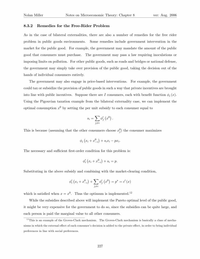
Nolan Miller Notes on Microeconomic Theory: Chapter 8 ver: Aug. 2006
8.3.2 Remedies for the Free-Rider Problem
As in the case of bilateral externalities, there are also a number of remedies for the free rider
problem in public goods environments. Some remedies include government intervention in the
market for the public good. For example, the government may mandate the amount of the public
good that consumers must purchase. The government may pass a law requiring inoculations or
imposing limits on pollution. For other public goods, such as roads and bridges or national defense,
the government may simply take over provision of the public good, taking the decision out of the
hands of individual consumers entirely.
The government may also engage in price-based interventions. For example, the government
could tax or subsidize the provision of public goods in such a way that private incentives are brought
into line with public incentives. Suppose there are I consumers, each with benefit function φi (x).
Using the Pigouvian taxation example from the bilateral externality case, we can implement the
optimal consumption x0 by setting the per unit subsidy to each consumer equal to
si =Xj 6=i
φ0j¡x0¢.
This is because (assuming that the other consumers choose x0j ) the consumer maximizes
φi¡xi + x0−i
¢+ sixi − pxi.
The necessary and sufficient first-order condition for this problem is:
φ0i¡xi + x0−i
¢+ si = p.
Substituting in the above subsidy and combining with the market-clearing condition,
φ0i¡xi + x0−i
¢+Xj 6=i
φ0j¡x0¢= p∗ = c0 (x)
which is satisfied when x = x0. Thus the optimum is implemented.12
While the subsidies described above will implement the Pareto optimal level of the public good,
it might be very expensive for the government to do so, since the subsidies can be quite large, and
each person is paid the marginal value to all other consumers.
12This is an example of the Groves-Clark mechanism. The Groves-Clark mechanism is basically a class of mecha-
nisms in which the external effect of each consumer’s decision is added to the private effect, in order to bring individual
preferences in line with social preferences.
227

Nolan Miller Notes on Microeconomic Theory: Chapter 8 ver: Aug. 2006
Lindahl Equilibrium
As in the bilateral externality case, both the quantity- and price-based government interventions
require the government to have detailed knowledge of the preferences of consumers and firms. We
now present a market-based solution to the problem, known as the Lindahl equilibrium. The idea
behind the Lindahl equilibrium is that the public good is unbundled into I private goods, where
each good is “person i’s enjoyment of the public good,” each with its own price (known as the
Lindahl price). The equilibrium in this market is known as the Lindahl equilibrium, and it turns
out that the Lindahl equilibrium implements the Pareto optimal allocation of the public good.
Suppose that for each i, there is a market for “person i’s enjoyment of the public good.” Denote
the price of this personalized good as pi. Given an equilibrium price, the consumer chooses the
total amount of the good to maximize
φi (x)− pixi,
which has necessary and sufficient first-order condition
φ0i (x) = pi for each i. (8.3)
Now, consider the producer side of the market. When the firm produces a single unit of the
public good, it produces one unit of the personalized public good for every person. That is, one
unit of national defense is a bundle of one unit of defense for person 1, one unit for person 2, etc.
Hence for each unit of the public good that the firm produces and sells, it earnsP
i pi dollars.
Hence the firm’s problem is written as
maxq
ÃXi
piq
!− c (q) ,
which has first-order condition Xi
pi = c0 (q) .
Combining this with the consumer’s optimality condition, Equation 8.3, yields
Xi
φ0i (q∗∗) = c0 (q∗∗) ,
which is the defining equation for the efficient level of the public good. The corresponding prices
are p∗∗i = φ0i (q
∗∗). Thus the Lindahl equilibrium results in the efficient level of the public good
being provided.
228

Nolan Miller Notes on Microeconomic Theory: Chapter 8 ver: Aug. 2006
The Lindahl equilibrium illustrates that the right kind of market can implement the Pareto
optimal allocation, even in the public good case. However, Lindahl equilibrium may not be
realistic. In particular, the Lindahl equilibrium depends on consumers behaving as price takers,
even when they are the only buyers of a particular good. Still, it may be reasonable to think that
the consumer has no power to force the producer of the public good to lower its price, especially
if the producer is the government. Second, and more troubling, is the idea that in order for the
Lindahl equilibrium to work, the consumer has to believe that if they do not purchase any of the
public good, they will not be able to consume any of it. Of course, since one of the defining features
of a public good is that it is non-excludable, it is unlikely that consumers will believe this.
8.3.3 Club Goods
However, while Lindahl equilibria may not be reasonable for pure (non-excludable) public goods,
they are reasonable if the good is excludable, which we earlier called club goods. The Lindahl
price p∗∗i can then be thought of as the price of a membership in the “club,” i.e. the right for
access to the club good. In this case, the market will result in efficient provision of the club good
(although you still have to worry about the price-taker assumption).
8.4 Common-Pool Resources
A common-pool resource (CPR) is a good where consumption is rivalrous and non-excludable.
Some of the prototypical examples of CPRs are local fishing grounds, common grazing land, or
irrigation systems. In such situations, individuals will tend to overuse the CPR since they will
choose the level of usage at which the individual marginal utility is zero, but the Pareto optimum is
the level at which the total marginal benefit is zero, which is generally a lower level of consumption
than the market equilibrium.
Consider the following example of a common-pool resource. The total number of fish caught
in a non-excludable local fishery is given by f (k), where k is the total number of fishing boats
that work the fishing ground. Assume that f 0 > 0 and f 00 < 0, and that f (0) = 0. That is, we
assume total fish production is an increasing concave function of the number of boats working the
fishing ground. Also, note that as a consequence of the concavity of f (), f(k)k > f 0 (k). That is,
the number of fish caught per boat is always larger than the marginal product of adding another
boat. This follows from the observation that average product is decreasing for a concave production
229

Nolan Miller Notes on Microeconomic Theory: Chapter 8 ver: Aug. 2006
function. Let AP (k) = f(k)k . Then AP 0 (k) = 1
k (f0 (k)−AP (k)) < 0. Hence AP (k) > f 0 (k).
Fishing boats are produced at a cost c (k), where k is the total number of boats, and c () is a
strictly increasing, strictly convex function. The price of fish is normalized to 1.
The Pareto efficient number of boats is found by solving
maxk
f (k)− c (k) ,
which implies the first-order condition for the optimal number of boats k0:
f 0¡k0¢= c0
¡k0¢.
Let ki be the number of boats that fisher i employs, and assume that there are I total fishers.
Hence k =P
i ki. If p is the market-clearing price of a fishing boat, the boat producers solve
maxk
pk − c (k) ,
which has optimality condition
c0 (k) = p.
Under the assumption that each fishing boat catches the same number of fish, each fisher solves
the problem
maxki
kiki + k−i
f (k)− pki,
where k−i =P
j 6=i kj . The optimality condition for this problem is
f 0 (k∗)k∗ik∗+
f (k∗)
k∗
µk∗−ik∗
¶= p.
Market clearing then implies that:
f 0 (k∗)k∗ik∗+
f (k∗)
k∗
µk∗−ik∗
¶= c0 (k∗) .
Since all of our producers are identical, the optimum will involve k∗i = k∗j for all i, j. That is, all
fishers will choose the same number of boats.13 If there are n total fishers, we can rewrite this
condition as:
f 0 (k∗)1
n+
f (k∗)
k∗
µn− 1n
¶= c0 (k∗) .
13 In fact, since f () is strictly concave, we could show this if we wanted to.
230

Nolan Miller Notes on Microeconomic Theory: Chapter 8 ver: Aug. 2006
Thus the left-hand side is a convex combination of the marginal product, f 0 (k), and the average
product, f(k)k . And, since we know that f(k)
k > f 0 (k), f 0 (k∗) 1n +f(k∗)k
¡n−1n
¢> f 0 (k∗). Finally,
since c0 (k) is increasing in k, this implies that k∗ > k0. The market overuses the fishery.
What causes people to overuse the CPR? Consider once again the fisher’s optimality condition:
f 0 (k∗)k∗ik∗+
f (k∗)
k∗
µk∗−ik∗
¶= p.
The terms on the left-hand side correspond to two different phenomena. First, if fisher i buys
another boat, that increases the total catch, and fisher i gets k∗ik∗ of that increase. This is the term
f 0 (k∗)k∗ik∗ . Second, because fisher i now has one more boat, he has a greater proportion of the total
boats, and so he gains from the fact that a greater proportion of the total catch is given to him.
This second effect, which corresponds to the term f(k∗)k∗
³k∗−ik∗
´, can be thought of as a “market
stealing” effect.
Note that both of these effects can lead the market to act inefficiently. Since the fisher only
gets k∗ik∗ of the increase in the number of fish due to adding another boat, this will tend to make
the market choose too few boats. However, since adding another boat also results in stealing part
of the catch from the other fishers, and this is profitable, this tends to make fishers buy too many
boats. When f () is concave, we know that the latter effect dominates the former, and there will
be too many boats.
The previous phenomenon, that the market will tend to overuse common-pool resources, is
known as the tragedy of the commons. We won’t have time to formally go through all of the
solutions to this problem, but they include the same sorts of tools that we have already seen. For
example, placing a quota on the number of boats each fisher can own or the number of fish that
each boat can catch would help to solve the problem. In addition, putting a tax on boats or fish
would also help to solve the problem. The appropriate boat tax would be
t∗ =k∗−ik∗
µf (k∗)
k∗− f 0 (k∗)
¶.
In this case, the fisher’s problem becomes:
maxki
kiki + k−i
f (k)− pki − t∗ki.
The first-order condition is:
f 0 (k)kik+
f (k)
k
µk−ik
¶− t∗ = p.
231
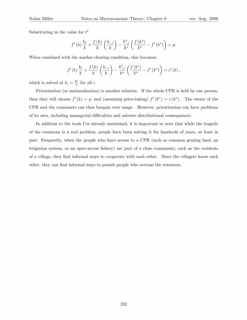
Nolan Miller Notes on Microeconomic Theory: Chapter 8 ver: Aug. 2006
Substituting in the value for t∗
f 0 (k)kik+
f (k)
k
µk−ik
¶−
k∗−ik∗
µf (k∗)
k∗− f 0 (k∗)
¶= p.
When combined with the market-clearing condition, this becomes:
f 0 (k)kik+
f (k)
k
µk−ik
¶−
k∗−ik∗
µf (k∗)
k∗− f 0 (k∗)
¶= c0 (k) ,
which is solved at ki = k∗
n for all i.
Privatization (or nationalization) is another solution. If the whole CPR is held by one person,
then they will choose f 0 (k) = p, and (assuming price-taking) f 0 (k∗) = c (k∗). The owner of the
CPR and the consumers can then bargain over usage. However, privatization can have problems
of its own, including managerial difficulties and adverse distributional consequences.
In addition to the tools I’ve already mentioned, it is important to note that while the tragedy
of the commons is a real problem, people have been solving it for hundreds of years, at least in
part. Frequently, when the people who have access to a CPR (such as common grazing land, an
irrigation system, or an open-access fishery) are part of a close community, such as the residents
of a village, they find informal ways to cooperate with each other. Since the villagers know each
other, they can find informal ways to punish people who overuse the resources.
232

Chapter 9
Monopoly
As you will recall from intermediate micro, monopoly is the situation where there is a single seller
of a good. Because of this, it has the power to set both the price and quantity of the good that
will be sold. We begin our study of monopoly by considering the price that the monopolist should
charge.1
9.1 Simple Monopoly Pricing
The object of the firm is to maximize profit. However, the price that the monopolist charges affects
the quantity it sells. The relationship between the quantity sold and the price charged is governed
by the (aggregate) demand curve q (p). Note, in order to focus on the relationship between q and
p, we suppress the wealth arguments in the aggregate demand function.
We can thus state the monopolist’s problem as follows:
maxp
pq (p)− c (q (p)) .
Note, however, that there is a one-to-one correspondence between the price charged and the quantity
the monopolist sells. Thus we can rewrite the problem in terms of quantity sold instead of the
price charged. Let p (q) be the inverse demand function. That is, p (q (p)) = p. The firm’s profit
maximization problem can then be written as
maxq
p (q) q − c (q) .
It turns out that it is usually easier to look at the problem in terms of setting quantity and letting
price be determined by the market. For this reason, we will use the quantity-setting approach.1References: Tirole, Chapter 1; MWG, Chapter 12; Bulow, “Durable-Goods Monopolists,” JPE 90(2) 314-332.
233

Nolan Miller Notes on Microeconomic Theory: Chapter 9 ver: Aug. 2006
A
D
Q Q0
P0
P
B
Figure 9.1: The Monopolist’s Marginal Revenue
In order for the solution to be unique, we need the objective function to be strictly concave (i.e.
d2πdq2
< 0). The second derivative of profit with respect to q is given by
d2
dq2(p (q) q − c (q)) = p00 (q) q + 2p0 (q)− c00 (q) .
If cost is strictly convex, c00 (q) > 0, and since demand slopes downward, p0 (q) < 0. Hence the
second and third terms are negative. Because of this, we don’t need inverse demand to be concave.
However, it can’t be “too convex.” Generally speaking, we’ll just assume that the objective function
is concave without making additional assumptions on p (). Actually, to make sure the maximizing
quantity is finite, we need to assume that eventually costs get large enough relative to demand.
This will always be satisfied if, for example, the demand and marginal cost curves cross.
The objective function is maximized by looking at the first derivative. At the optimal quantity,
q∗,
p0 (q∗) q∗ + p (q∗) = c0 (q∗)
On the left-hand side of the expression is the marginal revenue of increasing output a little bit.
This has two parts - the additional revenue due to selling one more unit, p (q∗) (area B in Figure
9.1), and the decrease in revenue due to the fact that the firm receives a lower price on all units it
sells (area A in Figure 9.1). Hence the monopolist’s optimal quantity is where marginal revenue
is equal to marginal cost, and price is defined by the demand curve p(q∗).2 See Figure 9.2 for the
graphical depiction of the optimum.
2This is also true for the competitive firm. However, since competitive firms are price takers, their marginal
revenue is equal to price.
234

Nolan Miller Notes on Microeconomic Theory: Chapter 9 ver: Aug. 2006
MC
D
MR
Q Q*
P*
P
Figure 9.2: Monopolist’s Optimal Price and Quantity
AC
D
MC
Q
P
Figure 9.3: The Monopolist Cannot Make a Profit
If the monopolist’s profit is maximized at q = 0, it must be that p (0) ≤ c0 (0). This corresponds
to the case where the cost of producing even the first unit is more than consumers are willing to pay.
We will generally assume that p (0) > c0 (0) to focus on the interesting case where the monopolist
wants to produce a positive output. However, even if we assume that p (0) > c0 (0), the monopolist
may not want to choose a positive output. It may be that shutting down is still preferable to
producing a positive output. That is, the monopolist may have fixed costs that are so large that it
would rather exit the industry. Such a situation is illustrated in Figure 9.3. Thus we interpret the
condition that p (0) > c0 (0) (along with the appropriate second-order conditions) as saying that if
the monopolist does not exit the industry, it will produce a positive output.
235

Nolan Miller Notes on Microeconomic Theory: Chapter 9 ver: Aug. 2006
If there is to be a maximum at a positive level of output, it must be that the first derivative
equals zero, or:
p0 (q∗) q∗ + p (q∗) = c0 (q∗)
Note that one way to rewrite the left side is:
p0 (q∗) q∗ + p (q∗) = p (q∗)
µdp
dq
q∗
p∗+ 1
¶= p (q∗)
Ã1− 1¯
ε∗p¯!
where ε∗p is the price elasticity of demand evaluated at (q∗, p∗). Now we can rewrite the monopolist’s
first-order condition as:p (q∗)− c0 (q∗)
p (q∗)= p0 (q∗)
−q∗p (q∗)
=1¯ε∗p¯ .
The left-most quantity in this expression, (p−mc) /p is the “markup” of price over marginal cost,
expressed as a fraction of the price. This quantity, called the Lerner index, is frequently used to
measure the degree of market power in an industry.
Note that at the quantity where MR = MC, p > MC (since p0 (q) q is negative). Thus the
monopolist charges more than marginal cost.3 The social optimum would be for the monopolist
to sell output as long as consumers are willing to pay more for the last unit produced than it costs
to produce it. That is, produce up until the point where p =MC. But, the monopolist cuts back
on production because it cares about profit, not social optimality. And, it is willing to reduce q in
order to increase the amount it makes per unit. This results in what is known as the deadweight
loss of monopoly, and it is equal to the area between the demand curve and the marginal cost
curve, and to the right of the optimal quantity, as in Figure 9.4. This area represents social surplus
that could be generated but is not in the monopoly outcome.
9.2 Non-Simple Pricing
The fact that the monopolist sells less than the societally optimal amount of the output arises from
the requirement that the monopolist must sell all goods at the same price. Thus if it wants to earn
higher profits on any particular item, it must raise the price on all items, which lowers the quantity
sold. If the monopolist could raise the price on some items but not others, it could earn higher
profits and still sell the efficient quantity. We now consider two examples of more complicated
pricing mechanisms along these lines, non-linear pricing and two-part tariffs.
3Also, from these two equations we can show that the monopolist will always choose a quantity such that price is
elastic, i.e. ε∗p > 1.
236
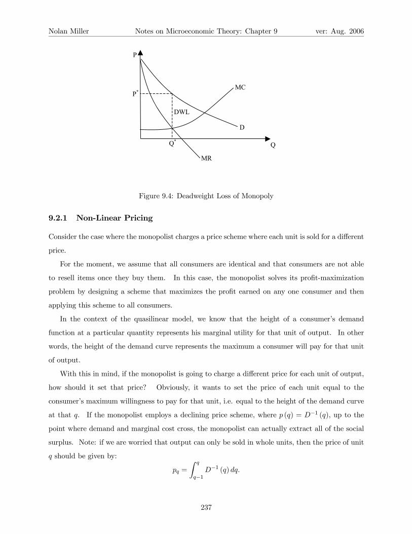
Nolan Miller Notes on Microeconomic Theory: Chapter 9 ver: Aug. 2006
MC
D
MR
Q Q*
P*
P
DWL
Figure 9.4: Deadweight Loss of Monopoly
9.2.1 Non-Linear Pricing
Consider the case where the monopolist charges a price scheme where each unit is sold for a different
price.
For the moment, we assume that all consumers are identical and that consumers are not able
to resell items once they buy them. In this case, the monopolist solves its profit-maximization
problem by designing a scheme that maximizes the profit earned on any one consumer and then
applying this scheme to all consumers.
In the context of the quasilinear model, we know that the height of a consumer’s demand
function at a particular quantity represents his marginal utility for that unit of output. In other
words, the height of the demand curve represents the maximum a consumer will pay for that unit
of output.
With this in mind, if the monopolist is going to charge a different price for each unit of output,
how should it set that price? Obviously, it wants to set the price of each unit equal to the
consumer’s maximum willingness to pay for that unit, i.e. equal to the height of the demand curve
at that q. If the monopolist employs a declining price scheme, where p (q) = D−1 (q), up to the
point where demand and marginal cost cross, the monopolist can actually extract all of the social
surplus. Note: if we are worried that output can only be sold in whole units, then the price of unit
q should be given by:
pq =
Z q
q−1D−1 (q) dq.
237

Nolan Miller Notes on Microeconomic Theory: Chapter 9 ver: Aug. 2006
Figure 9.5: Non-Linear Pricing
To illustrate non-linear pricing, consider a consumer who has demand curve P = 100−Q, and
suppose the monopolist’s marginal cost is equal to 10. At a price of 90, the consumer demands 10
units of output. While the consumer would not purchase any more output at a price of 90, it would
purchase more output if the price were lower. So, suppose the monopolist sells the first 10 units of
output at a price of 90, and the second 10 units at a price of 80. Similarly, suppose the monopolist
sells units 21-30 at a price of 70, 31-40 at a price of 60, 41-50 at a price of 50, etc., all the way up
to units 71-80, which are sold at a price of 20. This yields Figure 9.5.
The monopolist’s producer surplus is equal to the shaded region. Thus by decreasing the price
as the number of units purchased increases, the monopolist can appropriate much of the consumer
surplus. In fact, as the number of “steps” in the pricing scheme increases, the producer surplus
approaches the entire triangle bounded by the demand curve and marginal cost. Thus if the
monopolist were able to charge the consumerR qq−1D
−1 (q) dq for the block of output consisting of
unit q, it would appropriate the entire consumer surplus.
In practice, declining block pricing is found most often in utility pricing, where a large buyer
may be charged a high price for the first X units of output, a lower price for the next X units, and
so on.
Recall that we said that a monopolist charging a single price can make a positive profit only
if the demand curve is above the firm’s average total cost (ATC) curve at some point. If the firm
can engage in non-linear pricing, this is no longer the case. Since the firm’s revenue is the entire
shaded region in the above diagram, it may be possible for the firm to earn a positive profit even if
the demand curve is entirely below the ATC curve. For example, if ATC in the previous example
238

Nolan Miller Notes on Microeconomic Theory: Chapter 9 ver: Aug. 2006
Figure 9.6: Profit Even With Demand Below ATC
is as in Figure 9.6, then the monopolist can make a profit whenever the area of the shaded region
is larger that TC(90) = ATC(90)× 90.
9.2.2 Two-Part Tariffs
Another form of non-simple pricing that is frequently employed is the two-part tariff. A two-part
tariff consists of a fixed fee and a price per unit consumed. For example, an amusement park may
charge an admission fee and a price for each ride, or a country club may charge a membership fee
and a fee for each round of golf the member plays. The question we want to address is how, in
this context, the fixed fee (which we’ll call F ) and the use fee (which we’ll call p) should be set.
As in the non-linear pricing example, we continue to assume that all consumers are identical
and that the monopolist produces output at constant marginal cost. For simplicity, assume that
MC = 0, but note that a positive marginal cost is easily incorporated into the model. Further,
we continue to think of the consumer as having quasilinear utility for output q and a numeraire
good. In this case, we know that the consumer’s inverse demand curve, p (q), gives the consumer’s
marginal utility from consuming unit q, and that the consumer’s net benefit from consuming q
units is given by the consumer surplus at this quantity, CS (q).
The firm’s profit from two-part tariff (F, p) is given by F + p ∗ q (p). We break our analysis
into two steps. First, for any p, how should F be set? Second, which p should be chosen? So,
fix a p. How should F be set. Since the monopolist’s profit is increasing in F , the monopolist
wants to set F as large as possible while still inducing the consumer to participate. That is, the
consumer’s net benefit must be at least zero.
239

Nolan Miller Notes on Microeconomic Theory: Chapter 9 ver: Aug. 2006
q
p
qPO
p*
q(p*)
CS(p*)
PS(p*)
Figure 9.7: The Two-Part Tariff
At price p, the consumer chooses to consume q (p) units of output, and earns surplus CS (q (p)).
Net surplus is therefore CS (q (p))− F , and we want this to be non-negative: CS (q (p))− F ≥ 0.
As argued above, the firm wants to set F as large as possible. Therefore, for any p, setting
F (p) = CS (q (p)) maximizes profit. This makes sense, since the firm wants to set the membership
fee in order to extract all of the consumer’s surplus from using its product.
Next, how should p be chosen? Given F (p) as defined above, the monopolist’s profit from
the two-part tariff is given by: CS (q (p)) + p ∗ q (p) . Note that this is the sum of consumer and
producer surplus (see Figure 9.7). As is easily seen from the diagram, this expression is maximized
by setting the use fee equal to zero (marginal cost) and the fixed fee equal to CS (q (0)). Thus the
optimal two-part tariff involves p = 0 and F = CS (0).4
We can understand the optimal two-part tariff in another way. When the monopolist chooses
F optimally, it claims the entire surplus created from the market. Thus the monopolist has an
incentive to maximize the surplus created in this market. By the first welfare theorem, we know
that total surplus is maximized by the perfectly competitive outcome. That is, when p is such that
p∗ = MC. Thus, in order to maximize total surplus, the firm should set p = MC. If it does so,
“producer surplus” is zero. However, the firm sets F = CS(q (p∗), and extracts the entire social
surplus in the form of the fixed fee.
4More generally, if the firm has positive marginal cost, then p should be set such that p = MC at q (p), and F
should be set equal to CS (q (p)).
240

Nolan Miller Notes on Microeconomic Theory: Chapter 9 ver: Aug. 2006
Interestingly, there seems to be a trend toward this sort of two-part pricing in recent years. For
example, at Walt Disney World, the standard admission package charges for entry into one of the
several theme parks but charges nothing for rides once inside the park. This makes sense, since
the marginal cost of an additional ride is very low.5
9.3 Price Discrimination
Previously we considered the case where the monopolist faces one or many identical consumers,
and we investigated various pricing schemes the monopolist might pursue. However, typically, the
monopolist faces another problem, which is that some consumers will have a high willingness to
pay for the product and others will have a low willingness to pay. For example, business travellers
will be willing to pay more for airline tickets than leisure travellers, and working-age adults may
be more willing to pay for a movie ticket than senior citizens. We refer to the monopolist’s
attempts to charge different prices to these different groups of people as price discrimination.
Frequently, three types of price discrimination are identified, although the distinctions are, at least
to some extent, arbitrary. They are called first-degree, second-degree, and third-degree price
discrimination.6
9.3.1 First-Degree Price Discrimination
First-degree price discrimination - also called “perfect price discrimination” - refers to the situation
where the monopolist is able to sell each unit of output to the person that values it the most for their
maximum willingness to pay. For example, think of 100 consumers, each of whom have demand
for one unit of a good. Let p (q) be the qth consumer’s willingness to pay for the good (note, this
is just the inverse demand curve). A perfectly discriminating monopolist is able to charge each
consumer p (q) for the good: Each consumer is charged her maximum willingness-to-pay. In this
case, the monopolist’s marginal revenue is equal to p (q), and so the monopolist sets quantity q so
that p (q) = c0 (q), which is exactly the condition for Pareto optimality. Figure 9.8 depicts the
price-discrimination optimum, which is also the Pareto optimal quantity.
We can also think of first-degree price discrimination where each individual has a downward
5This contrasts with the scheme Disney used when I was younger, which involved both an admission fee and
positive prices for each ride. In fact, they even charged higher prices for the most popular rides.6There are many different definitions of the various kinds of price discrimination. The ones I use are based on
Varian’s Intermediate Microeconomics.
241
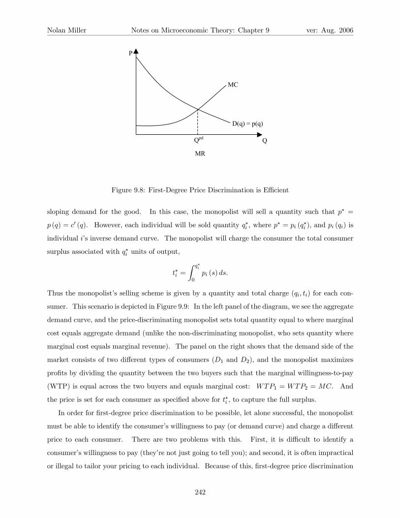
Nolan Miller Notes on Microeconomic Theory: Chapter 9 ver: Aug. 2006
MC
D(q) = p(q)
MR
Q Qpd
P
Figure 9.8: First-Degree Price Discrimination is Efficient
sloping demand for the good. In this case, the monopolist will sell a quantity such that p∗ =
p (q) = c0 (q). However, each individual will be sold quantity q∗i , where p∗ = pi (q
∗i ), and pi (qi) is
individual i’s inverse demand curve. The monopolist will charge the consumer the total consumer
surplus associated with q∗i units of output,
t∗i =
Z q∗i
0pi (s) ds.
Thus the monopolist’s selling scheme is given by a quantity and total charge (qi, ti) for each con-
sumer. This scenario is depicted in Figure 9.9: In the left panel of the diagram, we see the aggregate
demand curve, and the price-discriminating monopolist sets total quantity equal to where marginal
cost equals aggregate demand (unlike the non-discriminating monopolist, who sets quantity where
marginal cost equals marginal revenue). The panel on the right shows that the demand side of the
market consists of two different types of consumers (D1 and D2), and the monopolist maximizes
profits by dividing the quantity between the two buyers such that the marginal willingness-to-pay
(WTP) is equal across the two buyers and equals marginal cost: WTP1 = WTP2 = MC. And
the price is set for each consumer as specified above for t∗i , to capture the full surplus.
In order for first-degree price discrimination to be possible, let alone successful, the monopolist
must be able to identify the consumer’s willingness to pay (or demand curve) and charge a different
price to each consumer. There are two problems with this. First, it is difficult to identify a
consumer’s willingness to pay (they’re not just going to tell you); and second, it is often impractical
or illegal to tailor your pricing to each individual. Because of this, first-degree price discrimination
242

Nolan Miller Notes on Microeconomic Theory: Chapter 9 ver: Aug. 2006
D
MC
P*
Q* D1 D2
MC
Q1*
Q1* + Q2
*
P P
Q
Figure 9.9: First-Degree Price Discrimination
is perhaps best thought of as an extreme example of the maximum (but rarely attainable) profit
the monopolist can achieve.
9.3.2 Second-Degree Price Discrimination
Second-degree price discrimination refers to the case where the monopolist cannot perfectly identify
the consumers. For example, consider a golf course. Some people are going to use a golf course
every week and are willing to pay a lot for each use, while others are only going to use the course
once or twice a season and place a relatively low value on a round of golf. The owner of the golf
course would like to charge a high price to the high-valued users, and a low price to the low-valued
users. What’s the problem with this? On any given day, people will have an incentive to act
like low-valued users and pay the lower price. So, in order to be able to charge the high-valued
people a high price and the low-valued people a low price, the monopolist needs to design a pricing
scheme such that the high-valued people do not want to pretend to be low-valued people. This
practice goes by various names, including second-degree price discrimination, non-linear pricing,
and screening.
Let’s think about a simple example.7 Suppose the monopolist has zero marginal cost, and the
demand curves for the high- and low-valued consumers are given by DH (p) and DL (p). Assume
for the moment that there are equal numbers of high- and low-valued buyers. This scenario is
depicted in Figure 9.10.
7This example is based on the analysis in Varian’s Intermediate Microeconomics.
243
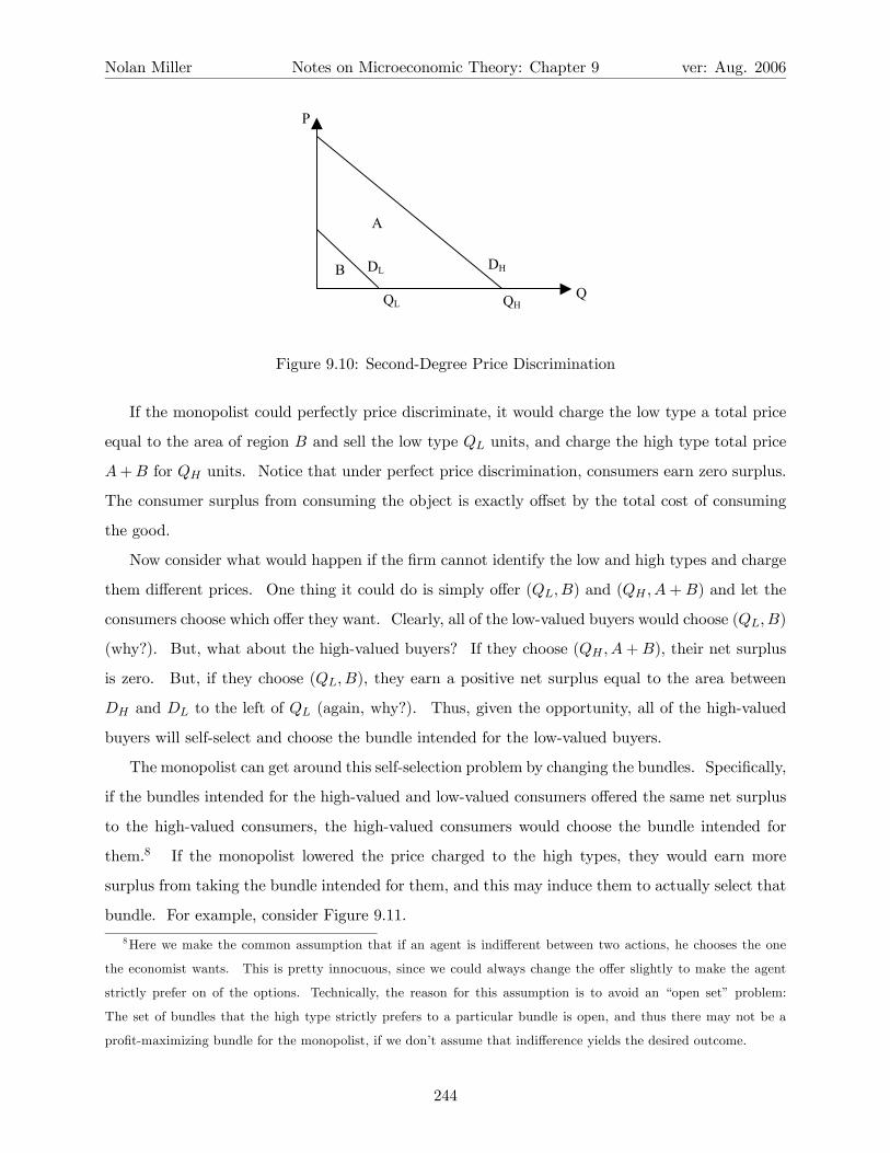
Nolan Miller Notes on Microeconomic Theory: Chapter 9 ver: Aug. 2006
P
Q
DHDL
A
B
QL QH
Figure 9.10: Second-Degree Price Discrimination
If the monopolist could perfectly price discriminate, it would charge the low type a total price
equal to the area of region B and sell the low type QL units, and charge the high type total price
A+B for QH units. Notice that under perfect price discrimination, consumers earn zero surplus.
The consumer surplus from consuming the object is exactly offset by the total cost of consuming
the good.
Now consider what would happen if the firm cannot identify the low and high types and charge
them different prices. One thing it could do is simply offer (QL, B) and (QH , A+B) and let the
consumers choose which offer they want. Clearly, all of the low-valued buyers would choose (QL, B)
(why?). But, what about the high-valued buyers? If they choose (QH , A+B), their net surplus
is zero. But, if they choose (QL, B), they earn a positive net surplus equal to the area between
DH and DL to the left of QL (again, why?). Thus, given the opportunity, all of the high-valued
buyers will self-select and choose the bundle intended for the low-valued buyers.
The monopolist can get around this self-selection problem by changing the bundles. Specifically,
if the bundles intended for the high-valued and low-valued consumers offered the same net surplus
to the high-valued consumers, the high-valued consumers would choose the bundle intended for
them.8 If the monopolist lowered the price charged to the high types, they would earn more
surplus from taking the bundle intended for them, and this may induce them to actually select that
bundle. For example, consider Figure 9.11.
8Here we make the common assumption that if an agent is indifferent between two actions, he chooses the one
the economist wants. This is pretty innocuous, since we could always change the offer slightly to make the agent
strictly prefer on of the options. Technically, the reason for this assumption is to avoid an “open set” problem:
The set of bundles that the high type strictly prefers to a particular bundle is open, and thus there may not be a
profit-maximizing bundle for the monopolist, if we don’t assume that indifference yields the desired outcome.
244

Nolan Miller Notes on Microeconomic Theory: Chapter 9 ver: Aug. 2006
A B
C D
E F G Q1 Q2 Q3 Q4
Figure 9.11: Monopolistic Screening
The optimal first-degree pricing scheme is to offer β1 = (Q3, E + F +G) to the low type
and β2 = (Q4, A+B +C +D +E + F +G) to the high type. However, high prefers β1, which
offers him surplus A + B + C to β2. In order to get the high-valued type to accept a bundle
offering Q4, the monopolist can charge no more than E + F + G + D. Let’s call this bundle
β3 = (Q4, E + F +G+D). If the monopolist has zero production costs, selling β3 to the highs
and β1 to the lows will be better than selling β1 to all consumers.
The key point in the previous paragraph is that the monopolist must design the bundles so that
the buyers self-select the proper bundle. If you want the highs to accept β3, it had better be that
there is no other bundle that offers them higher surplus.
The monopolist can do even better than offering β1 and β3. Suppose the monopolist offers
β4 = (Q2, E + F ) to low and β5 = (Q4, C +D +E + F +G) to high. Since high earns surplus
A + B from either bundle, the self-selection constraint is satisfied. The monopolist earns profit
C +D+2E +2F +G, as compared to 2E +2F +2G+D from offering β1 and β3. So, as long as
area C is larger than area G, the monopolist earns more profit from offering β4 and β5 than from
offering β1 and β3.
What is the optimal menu of bundles? In the previous paragraph, G is the revenue given up
by making less from the lows, while C is the revenue gained by making more from the highs. The
optimal bundle will be where these two effects just offset each other. In the diagram, they are
shown by β6 = (Q1, E) and β7 = (Q4, B + C +D +E + F +G).
Figure 9.12 gives a clean version of the diagrams we have been looking at above. The opti-
mal second-degree pricing scheme is illustrated. The monopolist should offer menu (Q∗L, A) and
245

Nolan Miller Notes on Microeconomic Theory: Chapter 9 ver: Aug. 2006
A
QL* QH
*
gain
loss B
C
p
q
D
Figure 9.12: Optimal Second-Degree Pricing Scheme
(Q∗H , A+B + C). Under this scheme, the low-valued consumers choose (Q∗L, A) and earn no sur-
plus. Notice that Q∗L is less than the Pareto optimal quantity for the low-valued consumers. The
high-valued consumers are indifferent between the two bundles, and so choose the one we want
them to choose: (Q∗H , A+B + C). Notice that under this scheme the high-valued consumers are
offered the Pareto optimal quantity, Q∗H , but earn a positive surplus. Overall, as the quantity
offered to the low-valued consumers decreases, the monopolist gains on the margin the area marked
“gain” in the diagram and loses the area market “loss.” The optimal level of Q∗L is where these
lengths are just equal.
Once we have derived the optimal second-degree pricing scheme, there is still one thing we have
to check. The monopolist could always decide it is not worth it to separate the two types of
consumers. Rather it could just offer Q∗H at price A+B + C +D in Figure 9.12 and sell only to
the high-valued consumers. Hence, after deriving the optimal self-selection scheme, we must still
make sure that the profit under this scheme, 2A+C+B, is greater than the profit from selling only
to the high types, A+B+C +D. Clearly, this depends on the relative size of A (the profit earned
by selling to the low-types under the optimal self-selection mechanism) and D (the rent that must
be given to the high type to get them to buy when offer (Q∗L, A) is also on the menu).9
The previous graphical analysis is different in style than you are used to. I show it to you for a
couple of reasons. First, it is a nice illustration of a type of problem that we will see over and over
again, called the monopolistic screening (or hidden-information principal-agent) problem.10 One
9 If there were different numbers of high- and low- type consumers, we would have to weight the size of the gains
and losses by the size of their respective markets.10Since you haven’t seen these other problems yet, this paragraph may not make sense to you. That’s okay. We’ll
246

Nolan Miller Notes on Microeconomic Theory: Chapter 9 ver: Aug. 2006
party (call her the principal) offers a menu of contracts to another party (call him the agent) about
which she does not know some information. The contracts are designed in such a way that the
agents self-select themselves, revealing that information to the principal. The menu of contracts
is distorted away from what would be offered if the principal knew the agent’s private information.
Further, it is done in a specific way. The high type is offered the full-information quantity, but
a lower price (phenomena like these are often referred to as “no distortion at the top” results),
while the low type is offered less than the full-information quantity at a lower price. Distorting
the quantity offered to the low type allows the principal to extract more profit from the high type,
but in the end the high type earns a positive surplus. This is known as the informational rent —
the extra payoff high gets due to the fact that the principal does not know his type.11 As I said,
this is a theme we will return to over and over again.
9.3.3 Third-Degree Price Discrimination
Third-degree price discrimination refers to a situation where the monopolist sells to different buyers
at different prices based on some observable characteristic of the buyers. For example, senior
citizens may be sold movie tickets at one price, while adults pay another price, and children pay
a third price. Self-selection is not a problem here, since the characteristic defining the groups is
observable and verifiable, at least in principle. For example, you can always check a driver’s license
to see if someone is eligible for the senior citizen price or not.
The basics of third-degree price discrimination are simple. In fact, you really don’t need to
know any economics to figure it out. Let p1 (q1) and p2 (q2) be the aggregate demand curves for
the two groups. Let c (q1 + q2) be the firm’s (strictly convex) cost function, based on the total
quantity produced. The monopolist’s problem is:
maxq1,q2
p1 (q1) q1 + p2 (q2) q2 − c (q1 + q2) .
come back to this point later.11This is only one type of principal-agent problem. Often, when people refer to “the” principal-agent problem, they
are referring to a situation where the agent makes an unobservable effort choice and the principal must design an
incentive contract that induces him to choose the correct effort level. To be precise, such models should be referred to
as “hidden-action principal-agent” models, to differentiate them from “hidden-information principal-agent” problems,
such as the monopolistic screening or second-degree price discrimination problems. See MWG Chapter 14 for a
discussion of the different types of principal-agent models.
247

Nolan Miller Notes on Microeconomic Theory: Chapter 9 ver: Aug. 2006
The first-order conditions for an interior maximum are:
p01 (q∗1) q
∗1 + p1 (q
∗1) = c0 (q∗1 + q∗2)
p02 (q∗2) q
∗2 + p2 (q
∗2) = c0 (q∗1 + q∗2) .
In general, you would need to check second-order conditions, but let’s just assume they hold. The
first-order conditions just say the monopolist should set marginal revenue in each market equal to
total marginal cost. This makes sense. Consider the last unit of output. If the marginal revenue
in market 1 is greater than the marginal revenue in market 2, you should sell it in market 1, and
vice versa. Hence any optimal selling scheme must set MR equal in the two markets. And, we
already know that MR should equal MC at the optimum.
So, third-degree price discrimination is basically simple. But, it can have interesting implica-
tions. For example, suppose there are two types of demand for Harvard football tickets. Alumni
have demand pa (qq) = 100 − qa, while students have demand ps (qs) = 20 − 0.1qs. Suppose the
marginal cost of an additional ticket is zero. How many tickets of each type should Harvard sell?
Set MR = MC in each market:
20− 0.2qs = 0
100− 2qa = 0,
So, q∗a = 50 and q∗s = 100 as well. Alumni tickets are sold at pa = 50, while student tickets are
sold at price ps = 10. Total profit is 50 ∗ 50 + 100 ∗ 10 = 2500 + 1000 = 3500.
Now, suppose that the stadium capacity is 151 seats (for the sake of argument), and that all
seats must be sold. Should the remaining seat be sold to alumni or students? Think of your
answer before going on.
If the additional seat is sold to alumni, qa = 51, pa = 49, and total profit on alumni sales is
2499, yielding total profit 3499. On the other hand, if the additional seat is sold to students,
qs = 101, ps = 20 − 0.1(101) = 9.9, total profit on student sales is 999.9, and so total profit is
3499.9. Hence it is better to sell the extra ticket to the students, even though the price paid by
the alumni is higher. Why? The answer has to do with marginal revenue. We know that in
either case selling another unit of output decreases total profit (why?). By selling an additional
alumni ticket, you have to lower the price more than when selling another student ticket. Hence
it is better to sell the ticket to a student, not because more is made on the additional ticket, but
because less is lost due to lowering price on the tickets sold to all other buyers in that market.
248
Nolan Miller Notes on Microeconomic Theory: Chapter 9 ver: Aug. 2006
9.4 Natural Monopoly and Ramsey Pricing
From the point of view of efficiency, monopolies are a bad thing because they impose a deadweight
loss.12 The government takes a number of steps to prevent monopolies. For example, patent law
grants a firm exclusive rights to an invention for a number of years in exchange for making the
design of the item available, and allowing other firms to license the use of the technology after a
period of time. Other ways the government opposes monopolies is through anti-trust legislation,
under which the government may break up a firm deemed to exercise too much monopoly power
(such as AT&T) or prevent mergers between competitors that would create monopolies..
However, there are some monopolies that the government chooses not to break up. Instead
the government allows the monopoly to operate (and even sanctions its operation) but regulates
the prices it can charge. Why would the government do such a thing? The government allows
monopolies to exist when they are so-called natural monopolies. A natural monopoly is an
industry where there are high fixed costs and relatively small variable costs. This implies that
AC will be decreasing in output. Because of this, it makes sense to have only one firm.13 The
best examples of natural monopolies are utilities such as the electric, gas, water, and (formerly)
telephone companies. Take the water company: In order to provide households with water, you
need to purify and filter the water and pass it through a network of pipes leading from the filtration
plant to the consumer’s house. The filtration plants are expensive to build, and the network of pipes
is expensive to install and maintain. Further, they are inconvenient, since laying and maintaining
pipe can disrupt traffic, businesses, etc. Think of how inefficient it would be if there were four or
five different companies all trying to run pipes into a person’s house!
Because of the inefficiency involved in having multiple providers in an industry that is a natural
monopoly, the government will allow a single firm to be the monopoly provider of that product, but
regulate the price that it is allowed to charge. What price does the government choose? Consider
the diagram of a natural monopolist in Figure 9.13.
12Of course, there are also critical distribution issues with monopolies, and these issues can persist even in situations
in which the DWL of monopoly has been eliminated. For example, with perfect price discrimination, there is no
DWL - the efficient quantity is sold - but the distribution of surplus (all to the monopolist, zero to consumers) is
clearly a cause for societal concern.13The technical definition of a natural monopoly is that the industry cost function is subadditive. That is,
c (q1 + q2) ≤ c (q1) + c (q2). Hence it is always cheaper to produce q1 + q2 units of output using a single firm than
using two (or more) firms. This is a slightly weaker definition of a natural monopoly than decreasing average cost,
especially in multiple dimensions.
249

Nolan Miller Notes on Microeconomic Theory: Chapter 9 ver: Aug. 2006
D
MR
AC
MC
PM
QM QR QE
PR
Figure 9.13: Ramsey Pricing
The monopolist has constant marginal cost, c0 (q) = MC, and positive fixed cost. Note that
this implies that AC > MC for all q, the defining feature of a natural monopolist.
If the monopoly is not regulated, it will charge price pM . The Pareto optimal quantity to sell is
where inverse demand equals marginal cost, labeled QE in the diagram. The corresponding price
is PE = MC. However, since this price is below AC, the monopolist will not be able to cover its
costs if the government forces it to charge PE. In order for the monopolist to cover its production
costs, it must be allowed to charge a higher price. However, as it increases price above MC, the
quantity drops below QE , and there is a corresponding deadweight loss. Thus the government’s
task is to strike a balance between allowing the monopolist to cover its costs and keeping prices
(and deadweight loss) low. The price that does this is the smallest price at which the monopolist
is able to cover its cost. This price is labeled PR in the diagram. The R stands for Ramsey, and
the practice of finding the prices that balance deadweight loss and allow the monopolist to cover
its costs is called Ramsey pricing. Finding the Ramsey price is easy in this example, but when the
monopolist produces a large number of products (such as electricity at different times of the day
and year, and electricity for different kinds of customers), the Ramsey pricing problem becomes
much harder.14 Ramsey pricing (and other related pricing practices) is one of the major topics in
the economics of regulation (or at least it was for a long time).15
14Ramsey pricing is really a topic for monopolists that produce multiple outputs. The Ramsey prices are then the
prices that maximize consumer surplus subject to the constraint that the firm break even overall.15Another type of regulatory mechanism is the regulatory-constraint mechanism, where the monopolist is allowed
250

Nolan Miller Notes on Microeconomic Theory: Chapter 9 ver: Aug. 2006
In recent years, technology has progressed to the point where many of the industries that
were traditionally thought to be natural monopolies are being deregulated. Most of these have
been “network” industries such as electric or phone utilities. Technological advances have made
it possible for a number of providers to use the same network. For example, a firm can generate
electricity and put it on the “power grid” where it can then be sold, or competing local exchange
carriers (phone companies) can provide phone service by purchasing access to Ameritech’s network
at prespecified rates.16 Because it is now possible for multiple firms to use the same network, these
industries are being deregulated, at least in part. Generally, the “network” remains a regulated
monopoly, with specified rates and terms for allowing access to the network. Provision of services
such as electricity generation or connecting phone calls is opened up to competition.
9.4.1 Regulation and Incentives
When a monopolist is regulated, the government chooses the output price so that the monopolist
just covers its costs.17 Because the monopolist knows that it will cover its costs, it will not have
an incentive to keep its costs low. As a result, it may incur costs that it would not incur if it were
subjected to market discipline. For example, it could purchase fancy office equipment, and decorate
the corporate headquarters. This phenomenon is sometimes known as gold plating. Gold-plating is
something regulators look out for when they are determining the cost base for the regulated firm.
An interesting phenomenon occurs when a firm operates both in a regulated and an unregulated
industry. For example, consider local phone providers, which are regulated monopolists on local
service (the “loop” from the switchbox to your house) but one of many competitors on “local toll”
calls (calls over a certain distance — like 15 miles). Since the firm knows it will cover its costs on
the local service, it may try to classify come of the costs of operating its competitive service as
costs of local service, thereby gaining a competitive advantage in the local toll market.
The extent to which the problems I mentioned here are real problems depend on the industry.
However, they are things that regulators worry about. Whenever a regulated monopoly goes before
a rate commission to ask for a rate increase, the regulators ask whether the costs are appropriate
to do whatever it wants, subject to a constraint such as its return on assets can be no larger than a pre-specified
number. If you are interested in such things, see Berg and Tschirhart, Natural Monopoly Regulation or Spulber,
Regulation and Markets.16Ameritech is the local phone company in the Chicago area, where I started writing these notes. In the Boston
area (where I’m adding this note), the relevant company is Verizon.17Actual regulation usually allows the firm to cover its costs and earn a specified rate of return on its assets.
251

Nolan Miller Notes on Microeconomic Theory: Chapter 9 ver: Aug. 2006
and whether they should be allocated to the regulated or competitive sector of the monopolist’s
business. The question of how regulated firms respond to regulatory mechanisms, i.e. regulatory
incentives, is another major subject in the economics of monopolies.
9.5 Further Topics in Monopoly Pricing
9.5.1 Multi-Product Monopoly
When a monopolist sells more than one product, it must take into account that the price it charges
for one of its products may affect the demand for its other products.18 This is true in a wide
variety of contexts, but let’s start with a simple example, that of a monopolist that sells goods that
are perfect complements. For example, think of a firm that sells vacation packages that consist
of a plane trip and a hotel stay. Consumers care only about the total cost of the vacation. The
higher the price of a hotel room, the less people will be willing to pay for the airline ticket, and
vice versa.
Demand for vacations is given by:
q (pV ) = 100− pV ,
where pV is the price of a vacation, pV = pA + pH , and pA and pH are the prices of airline travel
and hotel travel respectively. Each airline trip costs the firm cH , and each hotel stay costs cH .
To begin, consider the case where the firm realizes that consumers care only about the price of
a vacation, and so it chooses pV in order to maximize profit.
maxpV
(100− pV ) (pV − (cH + cA)) ,
since the cost of a vacation is cH + cA. The first-order condition for this problem is:
d
dpV((100− pV ) (pV − (cH + cA))) = 0
p∗V =100 + cH + cA
2= 50 +
cH + cA2
.
Thus if the firm is interested in maximizing total profit, it should set p∗V as above, and divide the
cost among the plane ticket and hotel any way it wants. In fact, if you’ve ever bought a tour, you
18See Tirole, Theory of Industrial Organization, starting at p. 70.
252

Nolan Miller Notes on Microeconomic Theory: Chapter 9 ver: Aug. 2006
know that you usually don’t get separate prices for the various components. Profit is given by:µ100− 100 + cH + cA
2
¶µ100 + cH + cA
2− cH − cA
¶=
1
4(100− (cH + cA))
2 .
Now consider the case where the price of airline seats and hotel stays are set by separate
divisions, each of which cares only about its own profits. In this case, the hotel division takes the
price of the airline division as given and chooses pH in order to maximize its profit:
(100− pH − pA) (pH − cH)
which implies that the optimal choice of pH responds to the airline price pA according to the
“reaction curve” or “best-response function” :
pH =100 + cH − pA
2.
Similarly, the airline division sets pA in order to maximize its profit, yielding reaction curve:
pA =100 + cA − pH
2.
At equilibrium, the optimal prices set by the two divisions must satisfy the two equation sys-
tem:19
pA =100 + cA − pH
2
pH =100 + cH − pA
2
which has solution:
p∗A =100 + 2cA − cH
3
p∗H =100− cA + 2cH
3
The total price of a tour is thus:
p∗H + p∗A =200 + cA + cH
3' 66.7 + cA + cH
3.
Unless cH + cA > 100 (in which case the cost of production is greater than consumers’ maximum
willingness to pay), the total price of a tour when the hotel and airline prices are set separately is
greater than the total price when they are set jointly, p∗V = 50 +cH+cA2 .
19This kind of best-response equilibrium is known in game theory as a Nash equilibrium - more on that in the game
theory chapters.
253

Nolan Miller Notes on Microeconomic Theory: Chapter 9 ver: Aug. 2006
When prices are set separately, the values of p∗H and p∗A above imply quantity:
100−µ200
3+1
3cA +
1
3cH
¶=
100
3− 13cA −
1
3cH
and total profit: µ100
3− 13cA −
1
3cH
¶µ200
3+1
3cA +
1
3cH − cH − cA
¶2
9(100− cH − cA)
2
Finally, since 29 < 1
4 , the firm earns higher profit when it sets both prices jointly than when the
prices are set independently by separate divisions.
The previous example shows that when the firm’s divisions set prices separately, they set the
total price too high relative to the prices that maximize joint profits. The firm as a whole would
be better off lowering prices — the increased demand would more than make up for the decrease in
price.
What is going on here? Begin with the case where the firm is charging p∗V , and suppose for
the sake of simplicity that the hotel price and airline price are equal. At p∗V , the marginal revenue
to the entire firm is equal to its marginal cost. That is,
MRFirm = 100− 2p∗V = cH + cA.
Now think about the incentives for the hotel manager in this situation. If the hotel increases its
price by a small amount, beginning from p∗V2 , its marginal revenue is:
MRHotel = 100− 2p∗H − p∗A = 100− 2p∗V2− p∗V2
> 100− 2p∗V =MRFirm.
Thus the hotel’s marginal gain in revenue due to raising its price is greater than the marginal gain
in revenue to the entire firm. Why? Raising the price reduces the quantity demanded, but the
increase in price all goes to the hotel, while the decrease in quantity is split between the hotel and
airline. But, the hotel manager doesn’t care about this latter effect on the airline. The same logic
holds for the airline manager’s choice of the airline price. Because of this, each division will charge
a price that is too high.
What about if the goods were substitutes instead of complements? Think about a car company
pricing its product line. If its lines are priced separately, each division head has an incentive to
254

Nolan Miller Notes on Microeconomic Theory: Chapter 9 ver: Aug. 2006
lower the price and steal some business from the other divisions. Because all division heads have
this incentive, the prices for the cars are lower when prices are set separately then they would be if
the firm set all prices centrally. This is sometimes known as cannibalization. The firm must worry
that by lowering the price on one line it is really just stealing business from the other product lines.
We will return to these types of issues when we study oligopoly. But, for now, we just want to
motivate the idea that even the monopolist has to worry about issues of strategy.20
9.5.2 Intertemporal Pricing
Consider the following scenario. A monopolist produces a single good that is sold in two consecutive
periods, 1 and 2. Using the quantity-based approach again, let p1 (q1) be the inverse demand curve
in the first period and p2 (q2, q1) be the inverse demand in the second period. Note that this
formulation indicates that the first-period demand does not depend on the second-period quantity.
This implies that first-period consumers do not plan ahead in their purchase decisions.
Let c1 (q1) and c2 (q2) be the cost functions in the two periods, with a discount factor δ = 11+r .
The monopolist maximizes:
p1 (q1) · q1 − c1 (q1) + δ (p2 (q2, q1) · q2 − c2 (q2))
The first-order conditions are:
p01 (q1) · q1 + p1 (q1) + δ
µ∂p2 (q2, q1)
∂q1· q2
= c01 (q1)
∂p2 (q2, q1)
∂q2· q2 + p2 (q2, q1) = c02 (q2)
Thus the monopolist sets marginal revenue equal to marginal cost in the second period. But,
what about the first period? In this period, the monopolist must take into account the effect of the
quantity sold in the first period on the quantity it will be able to sell in the second period. There
are two possible ways this effect could go:
• Goodwill: ∂p2(q2,q1)∂q1
> 0. Selling more in the first period generates “goodwill” that increases
demand in the second period, perhaps through reputation effects or good word-of-mouth. In
this case, the monopolist will produce more in the first period than it would if there were
only one period in the model (or if demand in the two periods were independent).
20Strategic issues are the main subject of the rest of these notes, starting with game theory, economists’ tool for
studying strategic interactions.
255

Nolan Miller Notes on Microeconomic Theory: Chapter 9 ver: Aug. 2006
• Fixed Pie: ∂p2(q2,q1)∂q1
< 0. Selling more in the first period means that demand is lower in the
second period. This would be true if the market for the product is fixed. In this case the
additional sales in period 1 are cannibalized from period 2, leaving nobody to buy in period
2. In this case, the monopolist will want to sell less than the amount it would in the case
where demand was independent in order to keep demand up in the second period.
Note - the stories told here are not quite rigorous enough. In Industrial Organization (IO)
economics, people work on models to account for these things explicitly. Our object here is to
illustrate that the firm’s strategy in the first period will depend on what the firm is going to do in
the second period.
9.5.3 Durable Goods Monopoly
Another way in which a monopolist can compete against itself is if it produces a product that is
durable. For example, think about a company that produces refrigerators. Substitute products
include not only refrigerators produced today by other firms, but refrigerators produced yesterday
as well. Put another way, the refrigerator is competing not only against other refrigerator makers,
it is also competing against past and future versions of its own refrigerator.
Consider the following simple model of a durable goods monopoly. A monopolist sells durable
goods that last forever. Each unit of the good costs c dollars. There are N consumers numbered
1,2,...,N. Consumer n values the durable good at n dollars. That is, she will pay up to n dollars,
but no more. Each day the monopolist quotes a price, pt, and agrees to sell the good to whomever
wants to purchase it at that price. How should the monopolist choose the path of prices? Assuming
no discounting, the monopolist is willing to wait, so it should charge price N on day 1, N − 1 on
day 2, etc. Each day, it skims off the highest value customers that remain. If there is a positive
discount rate, then the optimal price path will balance the extra revenue gained by skimming
against the cost of putting off the revenue of the lower valued customers into the future. Either
way, the monopolist is able to garner almost all the social surplus as profit. Can you think of
examples of this type of behavior? What about hard cover vs. soft cover books?
But, there is the problem with this model. If customers know that the price will be lower
tomorrow, they will wait to buy. Of course, how willing they are to wait will depend on the length
of the period. The longer they have to wait for the price to fall, the more likely they are to buy
today. We can turn the previous result on its head by asking what will happen as the length of
256

Nolan Miller Notes on Microeconomic Theory: Chapter 9 ver: Aug. 2006
the period gets very short. In this case, consumers will know that by waiting a very short time,
they can get the product at an even lower price. Because of this they will tend to wait to buy.
But, knowing that consumers will wait to buy, the monopolist will have an incentive to lower the
price even faster. The limit of this argument is that the monopolist is driven to charge p = MC
immediately, when the period is very short.
So, we have seen that the durable goods monopolist will make zero profit when it has the
opportunity to lower its price as fast as it wants to. This phenomenon is known as the Coase
Conjecture, so called because Coase believed it but didn’t prove it. It has since been proven.
Notice that the monopolist’s flexibility to charge different prices over time actually hurts the firm.
It would be better off if it could commit to charging the declining price schedule we mentioned
earlier. In fact, the monopolist would be better off if it could commit never to lower prices and
just charging the monopoly price forever. In this case, the firm wouldn’t sell any units in the
second period, but it would also face no pressures to lower the price in the first period.
How can a monopolist commit to never lowering its prices? The market gives us many examples:
• Print the price on the package
• Some products never go on sale by reputation, such as Tumi luggage
• Third-party commitment, such as using a retailer who is contractually prohibited from putting
items on sale
• “Destroy” the factory after producing in the first period, by limiting production runs (such
as “limited edition” collectibles or the “retirement” of Beanie Babies)
• Money back guarantee — if the price is lowered in the future, the monopolist will refund the
difference to all purchasers.
• Planned obsolescence — if the goods aren’t that durable, there isn’t a problem. In the
absence of an ability to commit to keeping prices high, firms should produce goods that
aren’t particularly durable.
• Leasing goods instead of selling them
This same phenomenon happens even in a two-period model. The monopolist would like to
charge a high price in both period. But after the first period has passed it has an incentive to
257

Nolan Miller Notes on Microeconomic Theory: Chapter 9 ver: Aug. 2006
lower the price in order to increase sales. But the customers, knowing that the monopolist will
lower prices in the second period, will not buy in the first period. Thus, the monopolist will have
to charge a lower price in the first period as well. The monopolist would be better off if it could
somehow commit to keeping prices high in both periods in this model.
Consider the following scenario. Instead of selling the durable good, the monopolist will lease
it for a year. In this case, units of the good rented in period 2 are no longer substitutes for units
of the good rented in period 1. In fact, somebody who likes the good will rent a unit in each year.
What should the monopolist do in this case? The monopolist should charge the monopoly
rental price (high price) in each period to rent the good. Thus if the monopolist can commit to
rental instead of selling, it can earn higher profits. Renting is similar to the other tools listed
above, in that it is an example of the firm’s intentionally restricting its own flexibility. Thus the
monopolist, by eliminating its opportunity to cut prices on sales later, is able to do better. In this
context, choice is not always a good thing.
Formal Model of Renting vs. Selling21 There are two periods, and goods produced in period
1 may be used in period 2 as well (i.e. it is durable). After period 2 the good becomes obsolete.
Assume that the cost of production is zero to make things simple, and the monopolist and consumers
have discount factor δ. Demand in each period is given by q (p) = 1 − p. The monopolist can
either lease the good for each period or sell it for both periods. If the monopolist decides to sell
the good, then consumers who purchased in the first period can resell it during the second period.
Suppose the monopolist decides to lease. The optimal price for the monopolist to charge in
each period is 1/2. This yields quantity 1/2 in the first period, which can be leased again in period
2. No additional quantity is produced in period 2. Thus discounted profits are given by
πlease =1
4(1 + δ)
Suppose the monopolist decides to sell. In this case, the quantity offered for sale in period 1
is reoffered by the resale market in period 2. Thus the residual demand in period 2 is given by
p2 = 1− q2 − q1. Thus in period 2 the monopolist chooses q2 to solve:
max q2 (1− q1 − q2)
which implies that the monopolist sells q2 =1−q12 and earns profit
³1−q12
´2.
21From Tirole, pp. 81-84.
258

Nolan Miller Notes on Microeconomic Theory: Chapter 9 ver: Aug. 2006
Now, what should the monopolist do in period 1? The price that consumers are willing to
pay is given by the willingness to pay in period 1 plus the discounted price in period 2, since the
consumer can always lease the object (or resell it) in period 2 for the market price. Thus consumers
are willing to pay
(1− q1) + δpa2
where pa2 is their belief about what the price will be in period 2.
We suppose that consumers correctly anticipate the price in the second period.22 That is,
pa2 = p2 =1−q12 . Thus as a function of q1 the maximum price the monopolist can charge is given
by:
p1 = (1− q1) + δ1− q12
= (1− q1)
µ1 +
δ
2
¶Thus in the first period the monopolist chooses q1 to maximize:
πsales = π1 + δπ2 = (1− q1)
µ1 +
δ
2
¶q1 + δ
µ1− q12
¶2The first-order condition yields:
d
dq1
Ã(1− q1)
µ1 +
δ
2
¶q1 + δ
µ1− q12
¶2!= 0
(1− q1)(1 +δ
2)− q1(1 +
δ
2)− δ(
1− q12
) = 0
q∗1 =2
4 + δ<1
2
q∗2 =1− q12
=1− 2
4+δ
2=1
2· 2 + δ
4 + δ
q∗1 + q∗2 =2
4 + δ+1
2· 2 + δ
4 + δ=1
2· 6 + δ
4 + δ>1
2
In terms of prices,
p∗2 = 1− (q∗1 + q∗2)
p∗2 =
µ1− 1
2· 6 + δ
4 + δ
¶=1
2· 2 + δ
4 + δ<1
2
p∗1 = (1− q1)
µ1 +
δ
2
¶=
µ1− 2
4 + δ
¶µ1 +
δ
2
¶=1
2
(2 + δ)2
4 + δ<1 + δ
2
22 In game theory terms, this is a Perfect Bayesian equilibrium.
259

Nolan Miller Notes on Microeconomic Theory: Chapter 9 ver: Aug. 2006
Note that 1+δ2 is the monopoly price if the second period is ignored (δ = 0). Going back to the
expression for total profit:
πsales = (1− q1)
µ1 +
δ
2
¶q1 + δ
µ1− q12
¶2=
1
2
(2 + δ)2
4 + δ· 2
4 + δ+ δ
µ1
2· 2 + δ
4 + δ
¶2=
µ2 + δ
4 + δ
¶2+ δ
µ1
2· 2 + δ
4 + δ
¶2= (1 +
δ
4)
µ2 + δ
4 + δ
¶2Comparing the sales profit, (1 + δ
4)³2+δ4+δ
´2, to the leasing profit, 14 (1 + δ), we can see that
πlease = πsales only when δ = 0. It turns out that for all δ > 0 (meaning the second period
matters, at least somewhat), then πlease > πsales. Leasing is more profitable. Why? When selling
the good, the monopolist cannot resist the temptation to lower the price in the second period and
sell more; thus, it cannot sell as much in the first period (q∗1 <12) as would be optimal, and this
reduces overall profits. The monopolist would be better off if it could commit to leasing rather
than selling.
260


