Lecture program

1. Space Astrometry 1/3: History, rationale, and Hipparcos

2. Space Astrometry 2/3: Hipparcos scientific results

3. Space Astrometry 3/3: Gaia

4. Exoplanets: prospects for Gaia

5. Some aspects of optical photon detection

Michael Perryman

1Friday, 15 November 13

Astrometry in the context of exoplanet detection/characterisation

groundspace

Protoplanetary/debris disks

Miscellaneous

10MJ

MJ

10M

M

Dynamical Photometry

existing capability projected (10–20 yr) discoveries follow-up detections n = planets known

173

39

244

8

Exoplanet DetectionMethods

Microlensing

decreasingplanet mass

Timing

15 planets(12 systems,2 multiple)

535 planets(403 systems,93 multiple)

2 planets(2 systems,0 multiple)

24 planets(22 systems,2 multiple)

Star accretion (?)

Collidingplanetesimals (1?)

Radio emission

X-ray emission (1)

417 planets(318 systems,68 multiple)

November 20131030 exoplanets

(784 systems, 170 multiple)[numbers from exoplanet.eu]

Astrometry Imaging

Transits

re!ectedlight

Rad velocity

free-!oating

optical radio

5

groundspace

subdwarfs

1

1

2

39 planets(36 systems,1 multiple)

photometricastrometric

Dopplervariability

bound

Discovered:

space(coronagraphy/interferometry)

ground(adaptive

optics)

timingresiduals

(see TTVs)

space

535 24

whitedwarfs

eclipsingbinaries

TTVs

pulsars

millisec

slow

Astrometry

2Friday, 15 November 13

Photometry

3Friday, 15 November 13

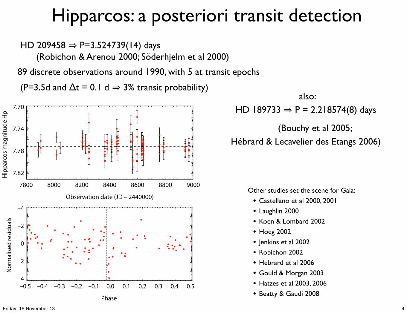
Hipparcos: a posteriori transit detection HD 209458 ⇒ P=3.524739(14) days (Robichon & Arenou 2000; Söderhjelm et al 2000)

89 discrete observations around 1990, with 5 at transit epochs

(P=3.5d and Δt = 0.1 d ⇒ 3% transit probability) also:

HD 189733 ⇒ P = 2.218574(8) days

(Bouchy et al 2005;Hébrard & Lecavelier des Etangs 2006)

Other studies set the scene for Gaia:

• Castellano et al 2000, 2001

• Laughlin 2000

• Koen & Lombard 2002

• Hoeg 2002

• Jenkins et al 2002

• Robichon 2002

• Hebrard et al 2006

• Gould & Morgan 2003

• Hatzes et al 2003, 2006

• Beatty & Gaudi 2008

–0.5 –0.4 –0.3 –0.2 –0.1 0.0 0.1 0.2 0.3 0.4 0.5

Phase

–4

–2

0

2

Nor

mal

ised

resid

uals

7800 8000 8200 8400 8600 8800 9000

Observation date (JD – 2440000)

7.70

7.74

7.78

7.82Hip

parc

os m

agni

tude

Hp

4

–0.5 –0.4 –0.3 –0.2 –0.1 0.0 0.1 0.2 0.3 0.4 0.5

Phase

–4

–2

0

2

Nor

mal

ised

resid

uals

7800 8000 8200 8400 8600 8800 9000

Observation date (JD – 2440000)

7.70

7.74

7.78

7.82Hip

parc

os m

agni

tude

Hp

4

4Friday, 15 November 13

Number of field of view transits

5Friday, 15 November 13

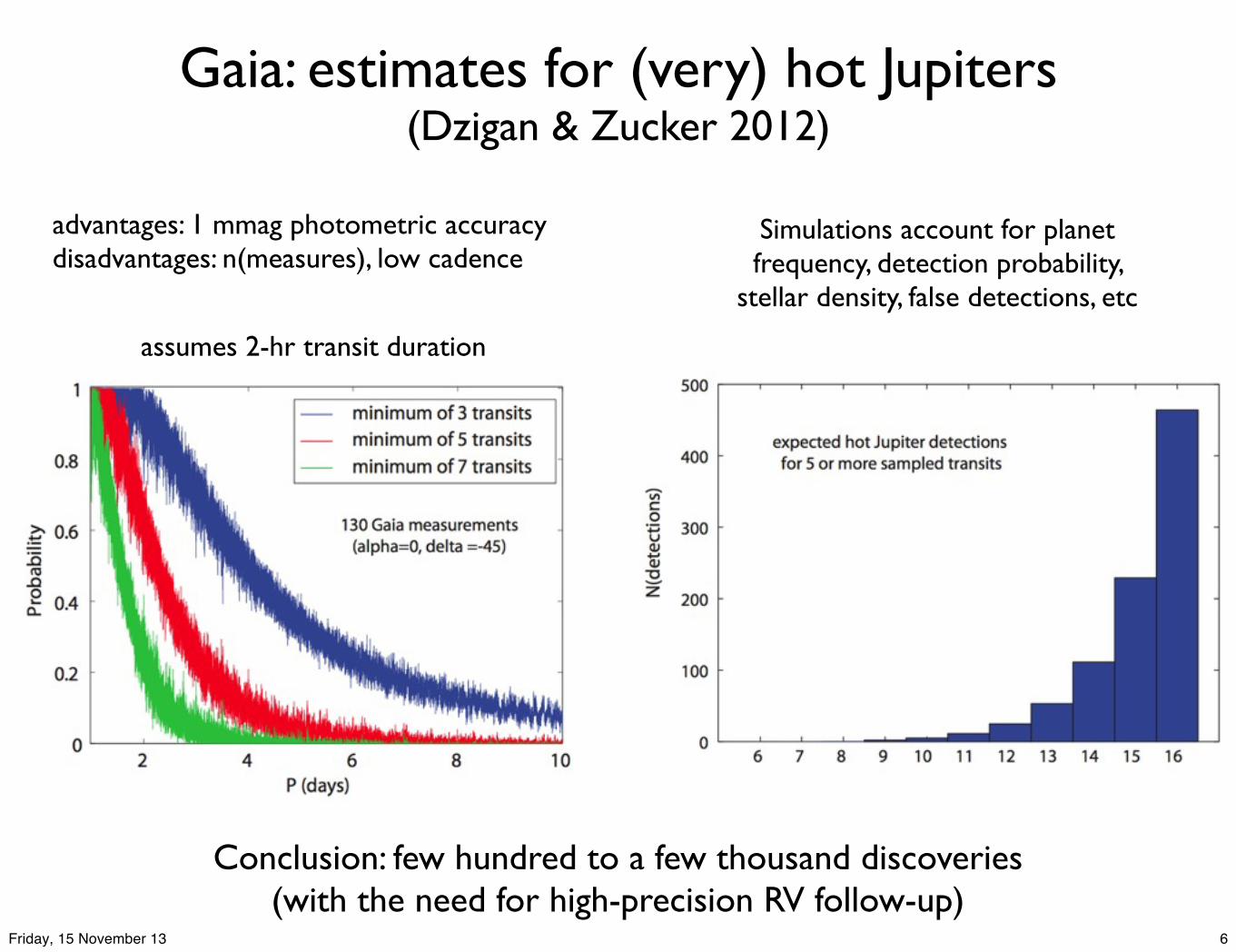
Gaia: estimates for (very) hot Jupiters(Dzigan & Zucker 2012)

Simulations account for planet frequency, detection probability,

stellar density, false detections, etc

advantages: 1 mmag photometric accuracydisadvantages: n(measures), low cadence

Conclusion: few hundred to a few thousand discoveries(with the need for high-precision RV follow-up)

assumes 2-hr transit duration

6Friday, 15 November 13

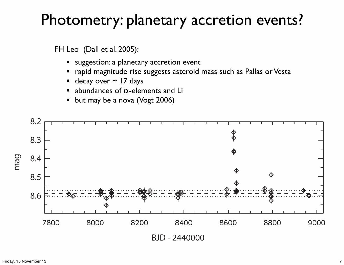
Photometry: planetary accretion events?

FH Leo (Dall et al. 2005):

• suggestion: a planetary accretion event• rapid magnitude rise suggests asteroid mass such as Pallas or Vesta• decay over ~ 17 days• abundances of α-elements and Li• but may be a nova (Vogt 2006)

mag

8.2

8.3

8.4

8.5

8.6

BJD - 2440000

7Friday, 15 November 13

Distances and space motions

8Friday, 15 November 13

Distances and motions

Examples:

• distances provide stellar parameters• e.g. transit planet diameters ∝ stellar diameters

• verification of seismology models for M, R

• proper motions characterise population(s) e.g. HIP 13044 low-metallicity Galactic halo stream (Helmi+1999, Setiawan+2010)

• Galactic birthplace based on metallicity-agee.g. Wielen (1996) inferred that the Sun’s birthplace was at R=6.6 kpc

9Friday, 15 November 13

Asteroseismology

Asteroseismology of η Boo, Z=0.04. Left: M=1.70±0.005 M⊙ Right: with overshooting

(Di Mauro et al 2003)

Can hope to discriminate:• primordial or self-enriched metallicity (bulk/surface): μ Ara (Pepe 2007), ι Hor (Laymand 2007)• planet radii calibrated wrt stellar radii: HAT-P-7 (Christensen-Dalsgaard+ 2010)• mass estimates cf isochrone models: β Gem, HD13189 (Hatzes+ 2008)• etc

For this, verification of the models by comparing parallax-based L with asteroseismology

10Friday, 15 November 13

Galactic birthplace (cont.)0.4

0.2

0

–0.2

–0.4

–0.6

–0.8

–1.0

[Fe/

H]

0 2 4 6 8 10 12 14 16

Age (Gyr)

Ri (kpc)

4.5

6.5

8.5

10.5

12.5

Sun

11Friday, 15 November 13

Hipparcos distances to exoplanet host stars

(a) (b)

50 pc 100 pc 50 pc 100 pc

100 brightest radial velocity host stars (end 2010)(versus RA, independent of dec)

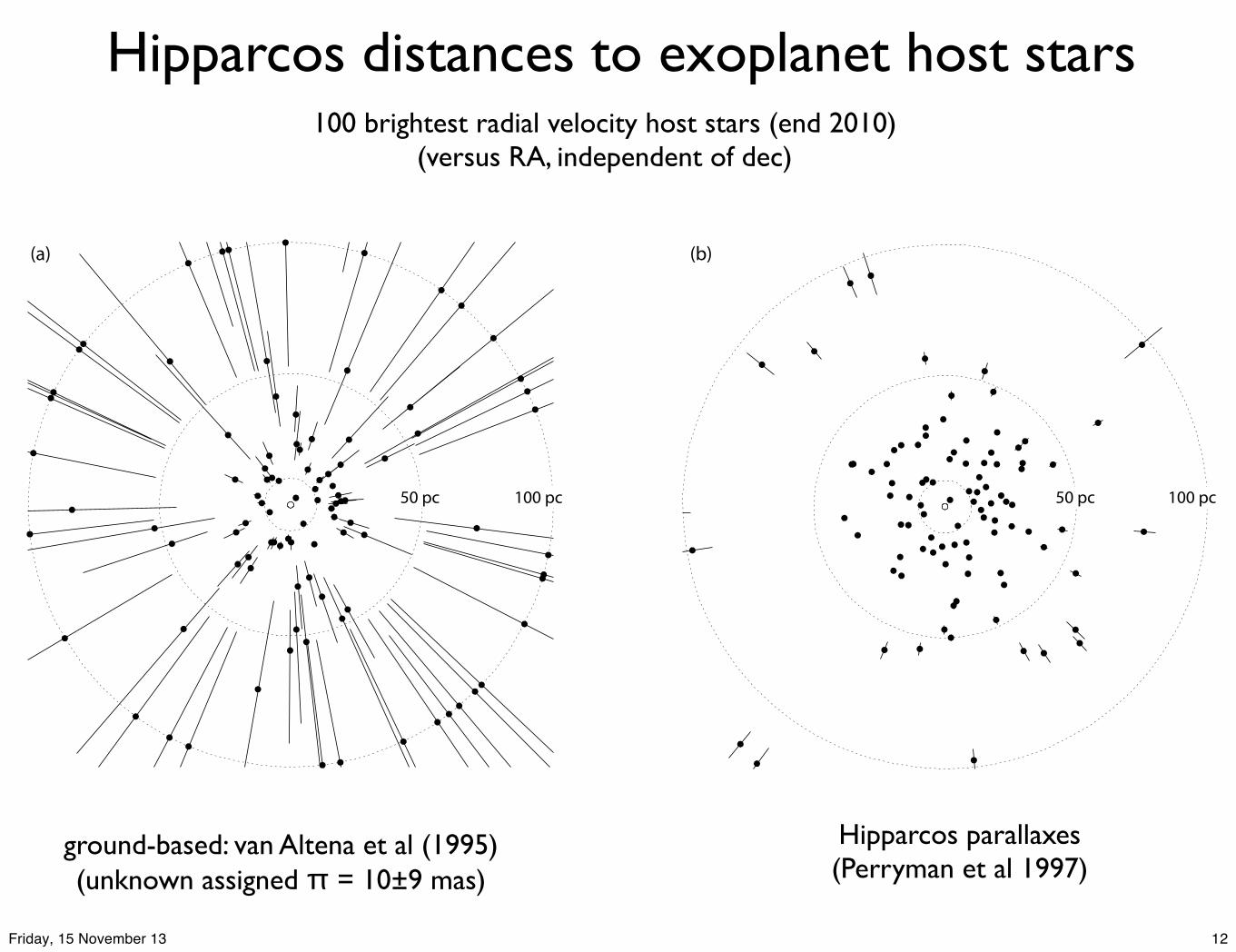
ground-based: van Altena et al (1995)(unknown assigned π = 10±9 mas)

Hipparcos parallaxes(Perryman et al 1997)

12Friday, 15 November 13

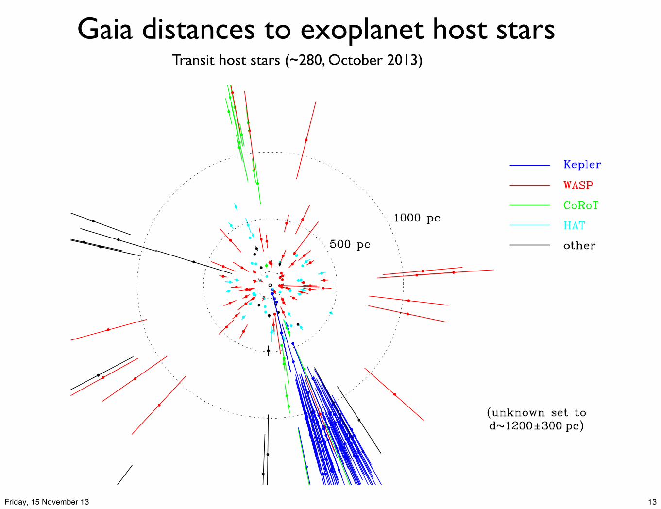
Gaia distances to exoplanet host starsTransit host stars (~280, October 2013)

13Friday, 15 November 13

New astrometric detections

14Friday, 15 November 13

Right ascension (mas)

Dec

linat

ion

(mas

)

0 50 100

150

0

50

100

2012.8

2011.6

2010.4

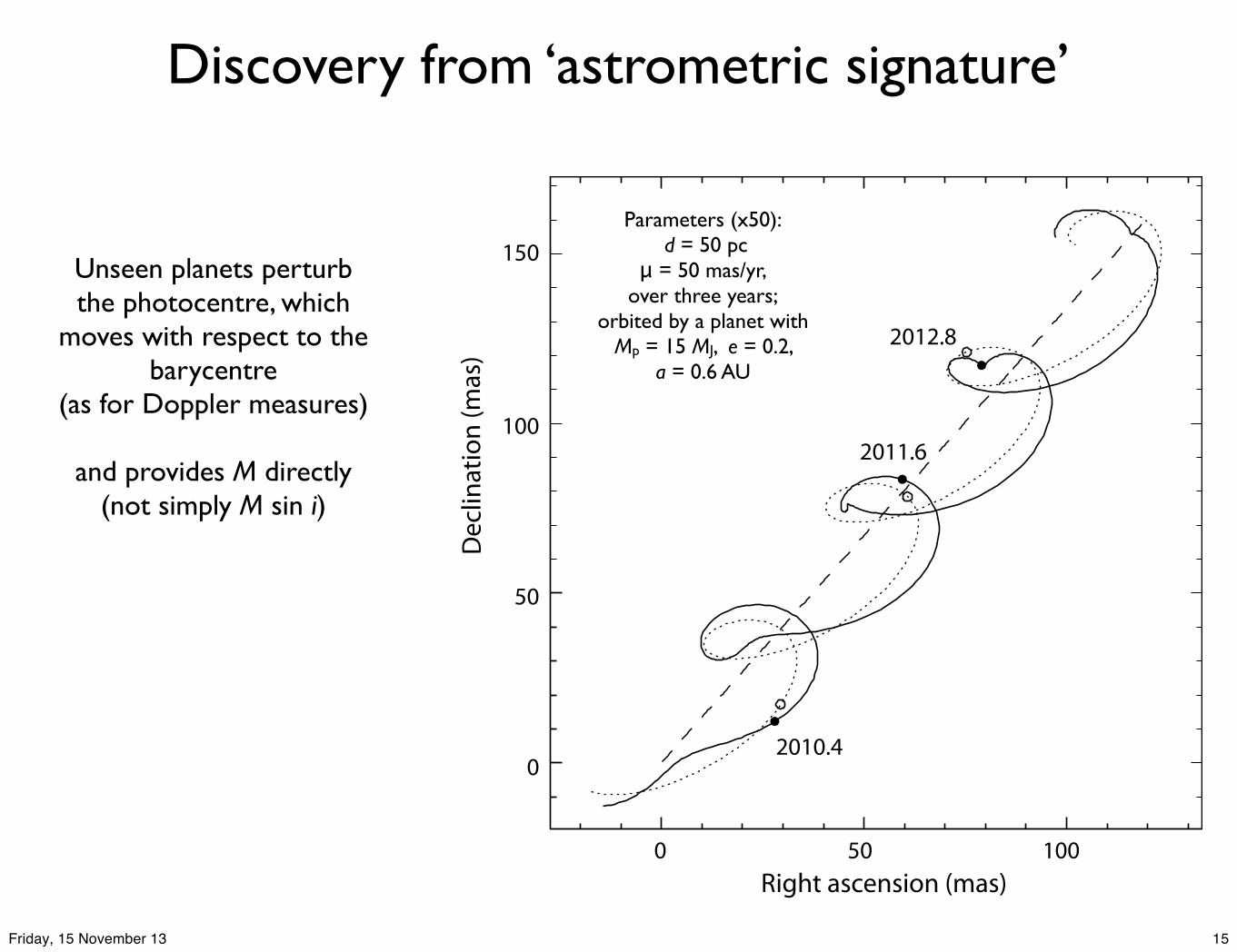
Unseen planets perturb the photocentre, which

moves with respect to the barycentre

(as for Doppler measures)

and provides M directly (not simply M sin i)

Discovery from ‘astrometric signature’

Parameters (x50): d = 50 pc

μ = 50 mas/yr,over three years;

orbited by a planet withMp = 15 MJ, e = 0.2,

a = 0.6 AU

15Friday, 15 November 13

Astrometric analysis: principles

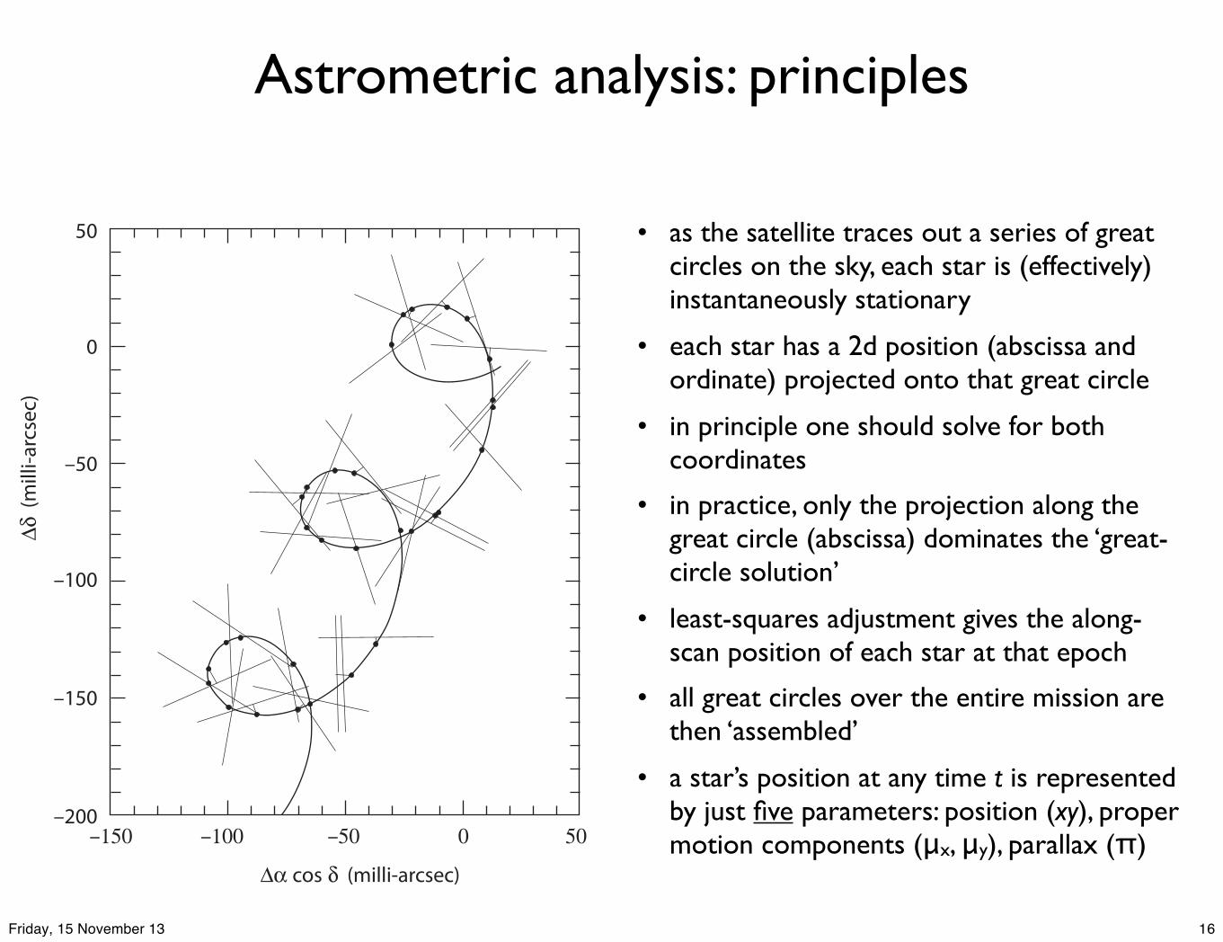
• as the satellite traces out a series of great circles on the sky, each star is (effectively) instantaneously stationary

• each star has a 2d position (abscissa and ordinate) projected onto that great circle

• in principle one should solve for both coordinates

• in practice, only the projection along the great circle (abscissa) dominates the ‘great-circle solution’

• least-squares adjustment gives the along-scan position of each star at that epoch

• all great circles over the entire mission are then ‘assembled’

• a star’s position at any time t is represented by just five parameters: position (xy), proper motion components (μx, μy), parallax (π)

50

–50

–50

–150

–150

–100

–100–200

0

0 50

!" cos # (milli-arcsec)

!# (milli-a

rcsec)

16Friday, 15 November 13

Direct access to planet mass

reference plane

ძ� �ascending node

i

orbit plane

!(t)

! =longitude of

ascending node

"! =

referencedirection

"to observer

orbitingbody pericentre

ellipse focus # centre of mass

rzწ� �descending

node

apocentre

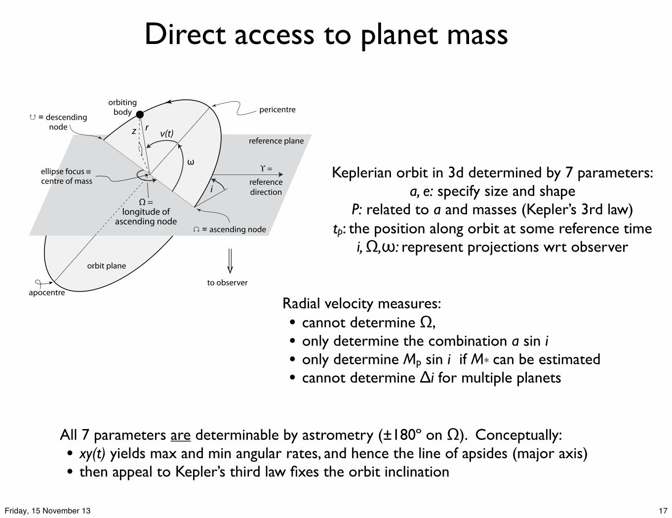
Keplerian orbit in 3d determined by 7 parameters:a, e: specify size and shape

P: related to a and masses (Kepler’s 3rd law)tp: the position along orbit at some reference time

i, Ω,ω: represent projections wrt observer

All 7 parameters are determinable by astrometry (±180º on Ω). Conceptually: • xy(t) yields max and min angular rates, and hence the line of apsides (major axis)• then appeal to Kepler’s third law fixes the orbit inclination

Radial velocity measures:• cannot determine Ω,• only determine the combination a sin i• only determine Mp sin i if M* can be estimated• cannot determine Δi for multiple planets

17Friday, 15 November 13

The ‘tragic history’ of astrometric planet detection

• Jacob (1855) 70 Oph: orbital anomalies made it ‘highly probable’ that there was a ‘planetary body’; supported by See (1895); orbit shown as unstable (Moulton 1899)

• Holmberg (1938): from parallax residuals... `Proxima Centauri probably has a companion’ of a few Jupiter masses

• Reuyl & Holmberg (1943) 70 Oph: planetary companion of ~10 MJ

• Strand (1943) 61 Cyg: companion of ~16 MJ

• lengthy disputes about planets around Barnard’s star: van der Kamp (1963, 1982)

• similarly for Lalande 21185 (e.g. Lippincott 1960)

• Pravdo & Shaklan (2009) vB10 with Palomar-STEPS, later disproved (Bean 2010)

• Muterspaugh+ (2010) HD~176051, only current detection: ‘may represent either the first such companion detected, or the latest in the tragic history of this challenging approach.’

• early discussions of space astrometry/Hipparcos exoplanet capabilities:

• Couteau & Pecker (1964), Gliese (1982)

18Friday, 15 November 13

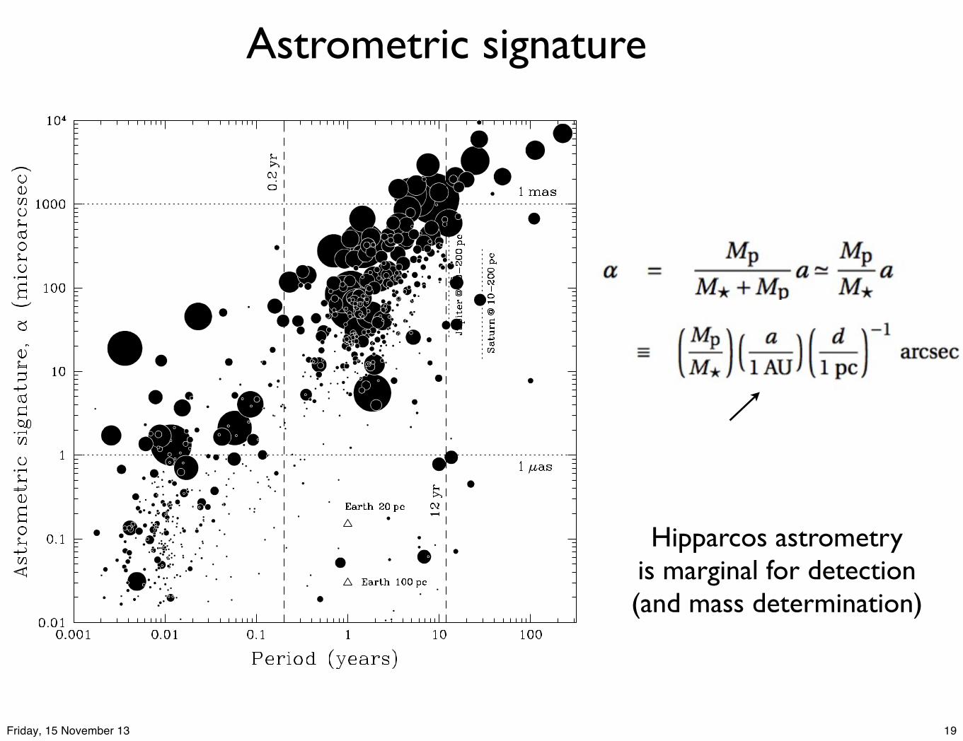
Astrometric signature

Hipparcos astrometryis marginal for detection(and mass determination)

19Friday, 15 November 13

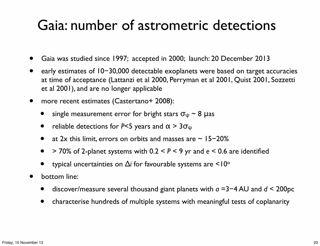
Gaia: number of astrometric detections

• Gaia was studied since 1997; accepted in 2000; launch: 20 December 2013

• early estimates of 10−30,000 detectable exoplanets were based on target accuracies at time of acceptance (Lattanzi et al 2000, Perryman et al 2001, Quist 2001, Sozzetti et al 2001), and are no longer applicable

• more recent estimates (Castertano+ 2008):

• single measurement error for bright stars σψ ~ 8 μas

• reliable detections for P<5 years and α > 3σψ

• at 2x this limit, errors on orbits and masses are ~ 15−20%

• > 70% of 2-planet systems with 0.2 < P < 9 yr and e < 0.6 are identified

• typical uncertainties on Δi for favourable systems are <10o

• bottom line:

• discover/measure several thousand giant planets with a =3−4 AU and d < 200pc

• characterise hundreds of multiple systems with meaningful tests of coplanarity

20Friday, 15 November 13

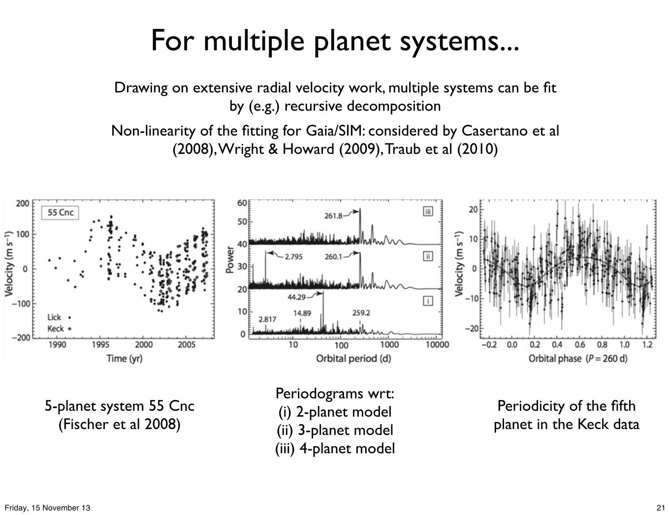
For multiple planet systems...Drawing on extensive radial velocity work, multiple systems can be fit

by (e.g.) recursive decomposition

Non-linearity of the fitting for Gaia/SIM: considered by Casertano et al (2008), Wright & Howard (2009), Traub et al (2010)

5-planet system 55 Cnc(Fischer et al 2008)

Periodograms wrt:(i) 2-planet model(ii) 3-planet model(iii) 4-planet model

Periodicity of the fifth planet in the Keck data

21Friday, 15 November 13

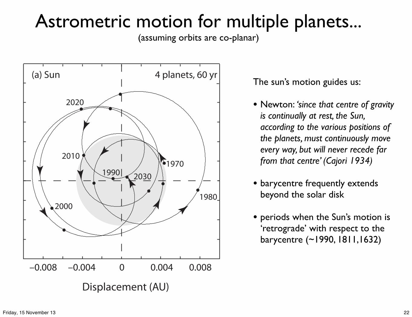
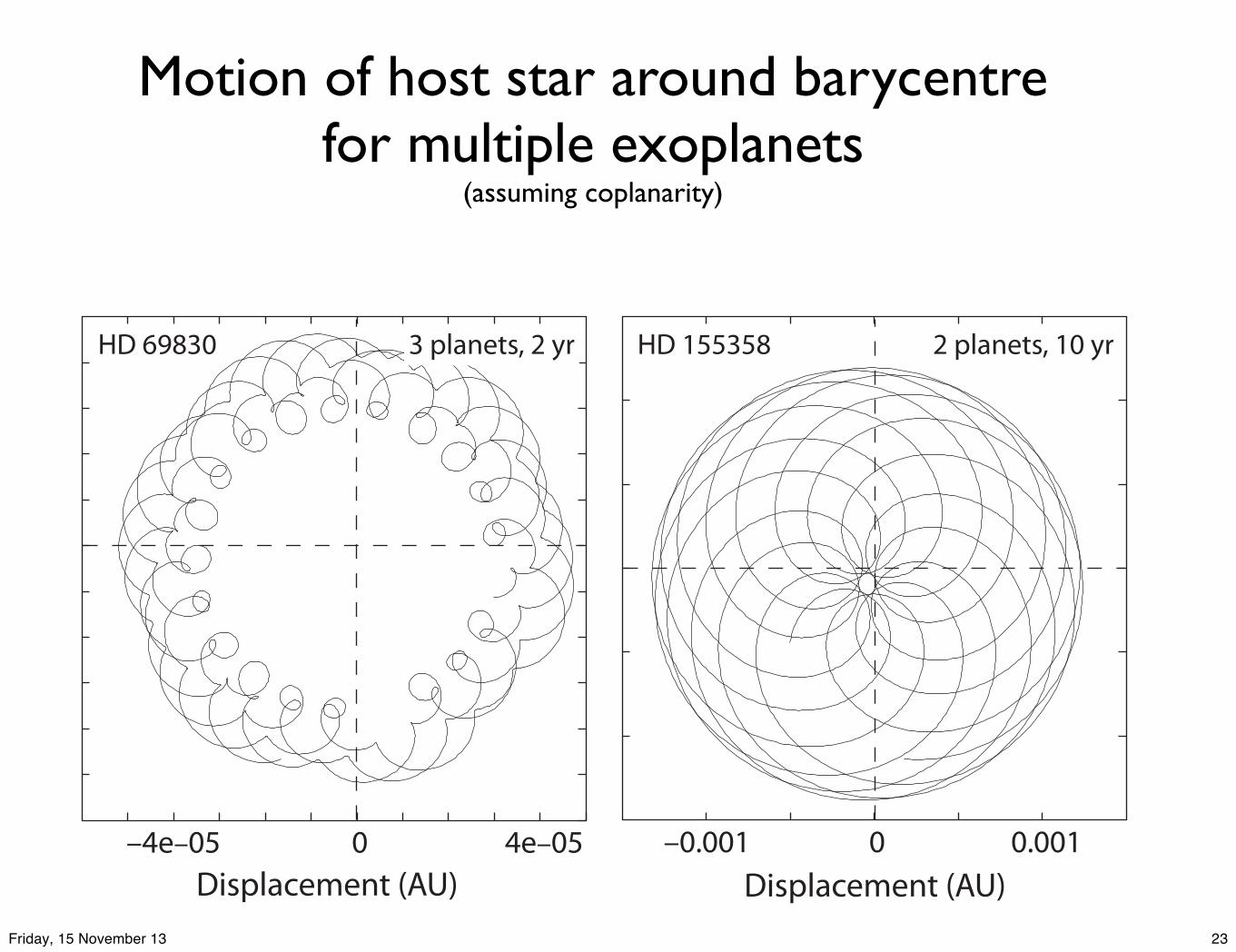
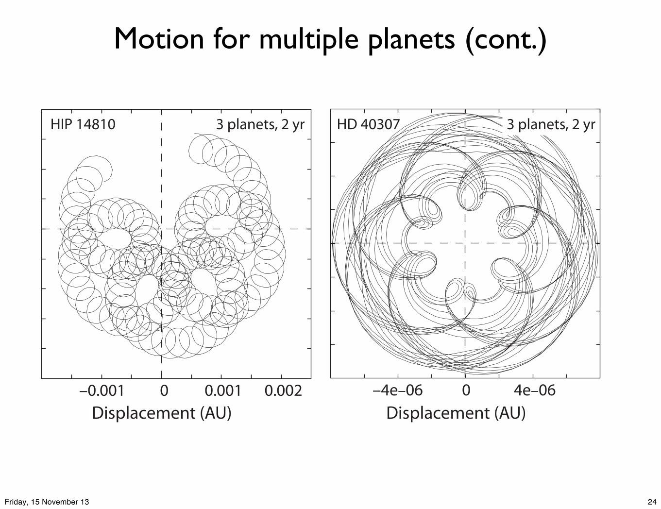
Astrometric motion for multiple planets...(assuming orbits are co-planar)

–0.01 0 0.01

(b) µ Ara

–0.002 0.002 0.004

(c) HD 371244 planets, 30 yr 3 planets, 30 yr

0

Displacement (AU)Displacement (AU)Displacement (AU)

–0.008 –0.004 0 0.004 0.008

(a) Sun

19702030

1980

1990

2000

2010

2020

4 planets, 60 yrThe sun’s motion guides us:

• Newton: ‘since that centre of gravity is continually at rest, the Sun, according to the various positions of the planets, must continuously move every way, but will never recede far from that centre’ (Cajori 1934)

• barycentre frequently extends beyond the solar disk

• periods when the Sun’s motion is ‘retrograde’ with respect to the barycentre (~1990, 1811,1632)

22Friday, 15 November 13

Motion of host star around barycentre for multiple exoplanets

(assuming coplanarity)

–0.001 0 0.001 0.002 –4e–06 0 4e–06 –4e–05 0 4e–05 –0.001 0 0.001

HIP 14810 HD 40307 HD 69830 HD 155358

Displacement (AU) Displacement (AU) Displacement (AU) Displacement (AU)

3 planets, 2 yr 2 planets, 10 yr3 planets, 2 yr 3 planets, 2 yr

23Friday, 15 November 13

Motion for multiple planets (cont.)

–0.001 0 0.001 0.002 –4e–06 0 4e–06 –4e–05 0 4e–05 –0.001 0 0.001

HIP 14810 HD 40307 HD 69830 HD 155358

Displacement (AU) Displacement (AU) Displacement (AU) Displacement (AU)

3 planets, 2 yr 2 planets, 10 yr3 planets, 2 yr 3 planets, 2 yr

24Friday, 15 November 13

Astronomia Nova (1609) includes Kepler’s hand drawing of the orbit of Mars viewed from Earth

...designated as ‘mandala’(Sanskrit for circle)

by Wolfram (2010)25Friday, 15 November 13

Exoplanets and the solar dynamo

26Friday, 15 November 13

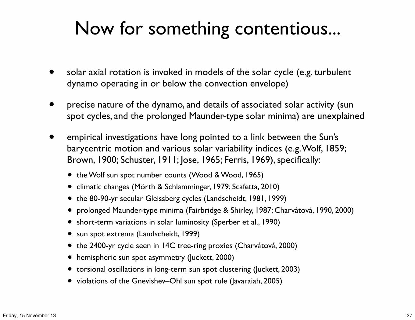
Now for something contentious...

• solar axial rotation is invoked in models of the solar cycle (e.g. turbulent dynamo operating in or below the convection envelope)

• precise nature of the dynamo, and details of associated solar activity (sun spot cycles, and the prolonged Maunder-type solar minima) are unexplained

• empirical investigations have long pointed to a link between the Sun’s barycentric motion and various solar variability indices (e.g. Wolf, 1859; Brown, 1900; Schuster, 1911; Jose, 1965; Ferris, 1969), specifically:

• the Wolf sun spot number counts (Wood & Wood, 1965)

• climatic changes (Mörth & Schlamminger, 1979; Scafetta, 2010)

• the 80-90-yr secular Gleissberg cycles (Landscheidt, 1981, 1999)

• prolonged Maunder-type minima (Fairbridge & Shirley, 1987; Charvátová, 1990, 2000)

• short-term variations in solar luminosity (Sperber et al., 1990)

• sun spot extrema (Landscheidt, 1999)

• the 2400-yr cycle seen in 14C tree-ring proxies (Charvátová, 2000)

• hemispheric sun spot asymmetry (Juckett, 2000)

• torsional oscillations in long-term sun spot clustering (Juckett, 2003)

• violations of the Gnevishev–Ohl sun spot rule (Javaraiah, 2005)

27Friday, 15 November 13

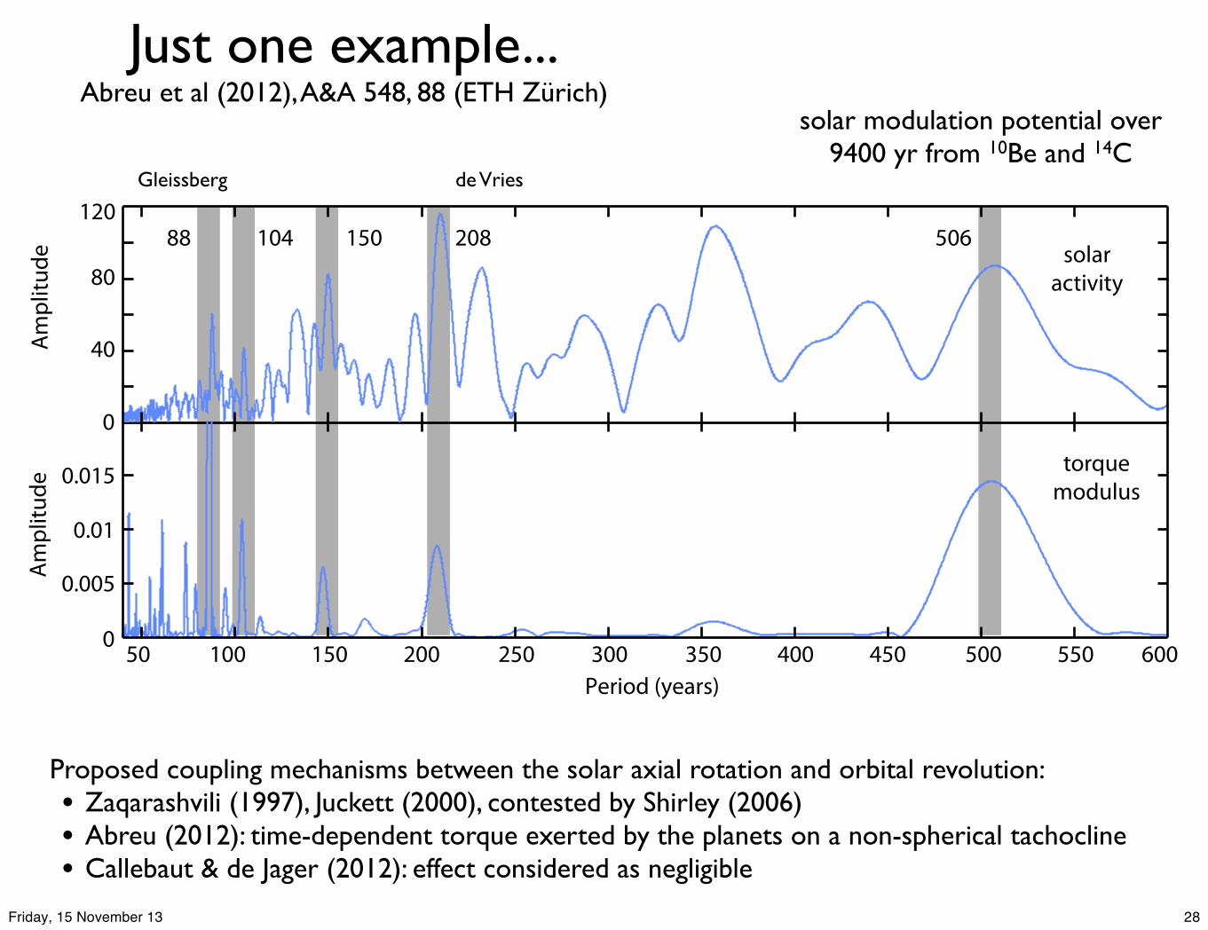
Just one example...Abreu et al (2012), A&A 548, 88 (ETH Zürich)

Proposed coupling mechanisms between the solar axial rotation and orbital revolution:• Zaqarashvili (1997), Juckett (2000), contested by Shirley (2006)• Abreu (2012): time-dependent torque exerted by the planets on a non-spherical tachocline• Callebaut & de Jager (2012): effect considered as negligible

50035030025020015010050 600550450400Period (years)

40

0

0.005

0.01

0.015

0

80

120

Ampl

itude

Ampl

itude

88 104 150 208 506solar

activity

torquemodulus

solar modulation potential over 9400 yr from 10Be and 14C

Gleissberg de Vries

28Friday, 15 November 13

Exoplanets can arbitrate(Perryman & Schulze-Hartung 2011)

• behaviour cited as correlated with the Sun’s activity includes

• changes in orbital angular momentum, dL/dt

• intervals of negative orbital angular momentum

• these are common (but more extreme) in exoplanet systems

• HD 168443 and HD 74156 have dL/dt exceeding that of the Sun by more than 105

• activity monitoring should therefore offer an independent test of the hypothetical link between:

• the Sun’s barycentric motion

• and the many manifestations of solar activity

29Friday, 15 November 13

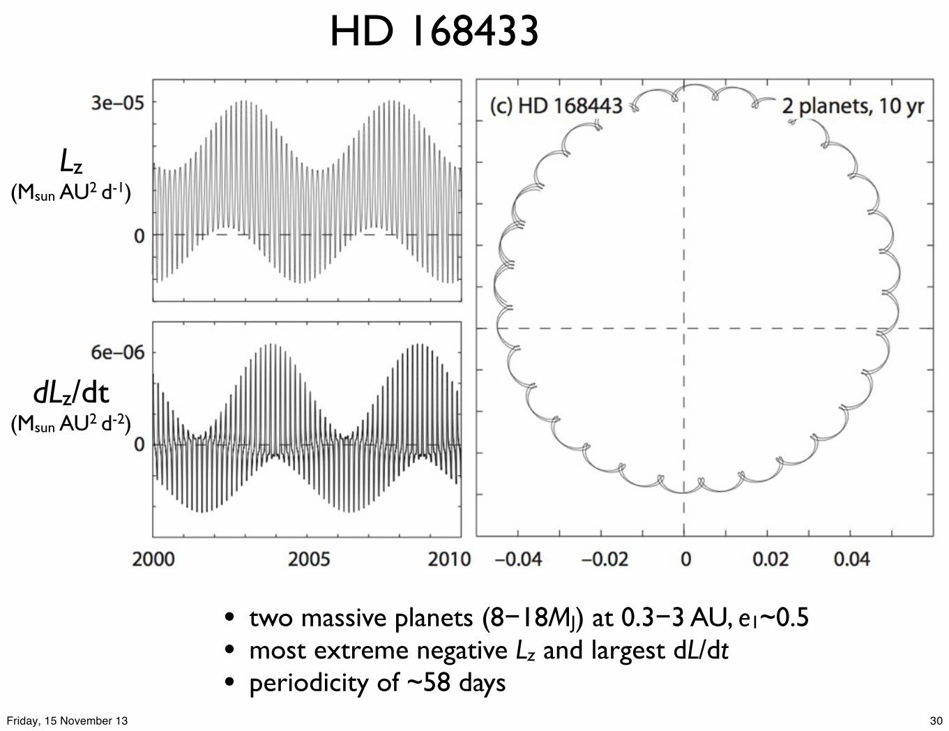
HD 168433

Lz(Msun AU2 d-1)

dLz/dt(Msun AU2 d-2)

• two massive planets (8−18MJ) at 0.3−3 AU, e1~0.5• most extreme negative Lz and largest dL/dt• periodicity of ~58 days

30Friday, 15 November 13

Coplanarity of orbitsand

transit geometry

31Friday, 15 November 13

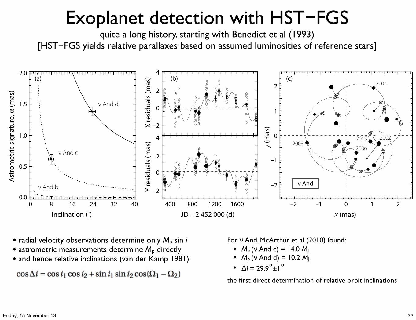
Exoplanet detection with HST−FGSquite a long history, starting with Benedict et al (1993)

[HST−FGS yields relative parallaxes based on assumed luminosities of reference stars]

Astr

omet

ric si

gnat

ure,

! (m

as)

Inclination (˚)0 8 16 24 32 40

JD – 2 452 000 (d) x (mas)

y (m

as)

Y re

sidua

ls (m

as)

X re

sidua

ls (m

as)

0

0

2

2

4

–2

–2

0

2

4

–2

0

2

–2

–1

–1

1

1400 800 1200 16000.0

0.5

1.0

1.5

2.0

! And d

! And c

! And b

2003

2004

2005

2006

2002

(a) (b) (c)

! And

For ν And, McArthur et al (2010) found:• Mp (ν And c) = 14.0 MJ

• Mp (ν And d) = 10.2 MJ

• Δi = 29.9°±1°the first direct determination of relative orbit inclinations

• radial velocity observations determine only Mp sin i• astrometric measurements determine Mp directly• and hence relative inclinations (van der Kamp 1981):

32Friday, 15 November 13

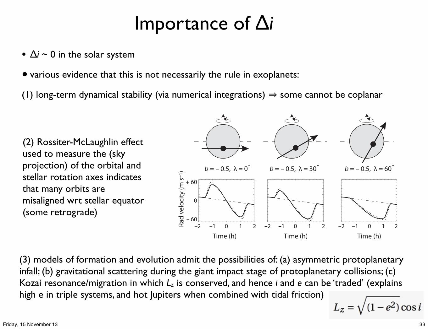
Importance of Δi

• Δi ~ 0 in the solar system

• various evidence that this is not necessarily the rule in exoplanets:

(1) long-term dynamical stability (via numerical integrations) ⇒ some cannot be coplanar

b = – 0.5, ! = 0" b = – 0.5, ! = 30" b = – 0.5, ! = 60"

Time (h)–2 –1 0 1 2

Time (h)–1 0 1 2

Time (h)–1 0 1 2–2 –2Ra

d ve

loci

ty (m

s#1)

+ 60

0

– 60

(2) Rossiter-McLaughlin effect used to measure the (sky projection) of the orbital and stellar rotation axes indicates that many orbits are misaligned wrt stellar equator (some retrograde)

(3) models of formation and evolution admit the possibilities of: (a) asymmetric protoplanetary infall; (b) gravitational scattering during the giant impact stage of protoplanetary collisions; (c) Kozai resonance/migration in which Lz is conserved, and hence i and e can be ‘traded’ (explains high e in triple systems, and hot Jupiters when combined with tidal friction)

33Friday, 15 November 13

0

5

10

15

20

2005 2006 2007 2008

J12

Year

observation particularly e!cient(ine!cient)

preceding observations

ๆๅ ๅ

observationsnot possible

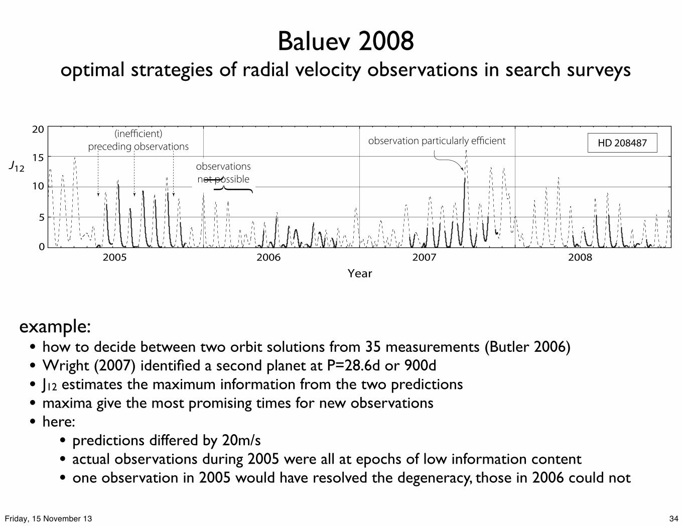
HD 208487

Baluev 2008optimal strategies of radial velocity observations in search surveys

example: • how to decide between two orbit solutions from 35 measurements (Butler 2006)• Wright (2007) identified a second planet at P=28.6d or 900d• J12 estimates the maximum information from the two predictions• maxima give the most promising times for new observations• here:

• predictions differed by 20m/s• actual observations during 2005 were all at epochs of low information content• one observation in 2005 would have resolved the degeneracy, those in 2006 could not

34Friday, 15 November 13

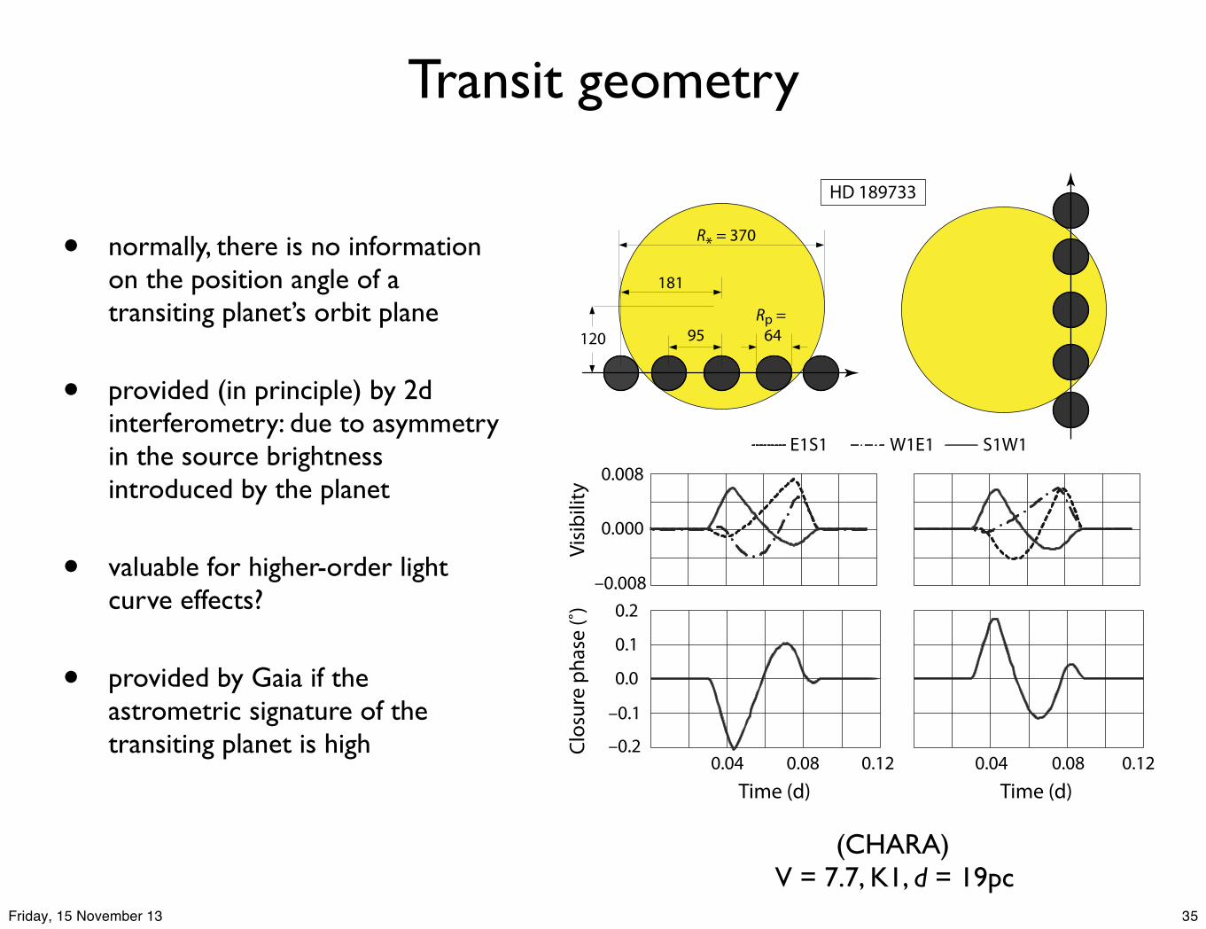
Transit geometry

• normally, there is no information on the position angle of a transiting planet’s orbit plane

• provided (in principle) by 2d interferometry: due to asymmetry in the source brightness introduced by the planet

• valuable for higher-order light curve effects?

• provided by Gaia if the astrometric signature of the transiting planet is high

0.04 0.08 0.12Time (d)

0.04 0.08 0.12Time (d)

0.008

0.000

–0.008Vi

sibili

tyCl

osur

e ph

ase

(˚) 0.2

0.1

0.0

–0.1

–0.2

E1S1 W1E1 S1W1

R* = 370

181

120 95Rp =

64

HD 189733

(CHARA) V = 7.7, K1, d = 19pc

35Friday, 15 November 13

Summary

• accurate distances:

• calibration of host star parameters, including R for transiting

• calibration of asteroseismology models

• accurate proper motions: Galactic dynamics and population

• multi-epoch high-accuracy photometry:

• new transiting systems (several hundred?)

• calibration of photometric jitter vs spectral type

• multi-epoch astrometry:

• discovery of new (massive, long-period) planets (3000?)

• co-planarity of systems: evolutionary models

• position angle of planet transits (some multiple?)

36Friday, 15 November 13

End

37Friday, 15 November 13