103
Business Statistics Prof. Lancelot JAMES Hong Kong University of Science and Technology, Information and Systems ManagemenT ISMT-551 _ Fall 2006
| Date post: | 23-Dec-2015 |
| Category: |
Documents |
| Upload: | satyasainadh |
| View: | 36 times |
| Download: | 0 times |
Business Statistics
Prof. Lancelot JAMES
Hong Kong University of Science and Technology,Information and Systems ManagemenT
ISMT-551 _ Fall 2006

Outline of the Course
Prerequisites-Good STAMINAClass Participation is EncouragedGrading: Homeworks/Projects and Final ExamTextbook: Bowerman, O’ Connell, Orris (2004) Essentialsof Business Statistics. Mc Graw Hill.Use the online tutorials
(http://highered.mcgraw-hill.com/sites/0072827823/student_view0/electronic_
tutorials.html)

Salutations
Prof/Dr. James
Introduction Descriptive Statistics
What is statistics?
The formal definition is simply the study or analysis of data.Statistics is a tool for studying a characteristic or a behavior inthe real world based on a sample from the entire population
1 DATA IS EVERYWHERE

Introduction Descriptive Statistics
How might statistics be used in a businesscontext?
1 To know how to present and describe information2 To know how to draw conclusions about large populations
based only on information obtained in samples3 To know how to improve processes4 To know how to obtain forecasts5 Making DECISIONS

Introduction Descriptive Statistics
Populations and samples
1 ParameterA summary measure that describes acharacteristic of an entire population. For example theaverage height of people in the US.
2 Sample A portion of the population that is selected foranalysis.
3 A Statistic: A summary measure computed from sampledata that is used to describe or estimate a characteristic ofthe entire population.
Introduction Descriptive Statistics
Populations and samples
Key Definitions
a Population is a set of existing units (people, objects,events,...)a Variable is any characteristic of a PopulationAll the population measurements may be collected in aCensus.a Sample is a subset of the units in the population.
A sample of measurements that can be1 Described ⇒ Descriptive Statistics2 Used to make generalizations about important aspects of
the Population ⇒ Statistical Inference

Introduction Descriptive Statistics
Populations and samples
Population vs. Sample

Introduction Descriptive Statistics
Populations and samples
Types of Data
Introduction Descriptive Statistics
Populations and samples
1. Population:Some Examples of a Population
All items or subjects under consideration.
1 The stars in the galaxy2 red cars, cars produced by Toyota in a given year3 People in ISMT551, HKUST, Hong Kong, Asia, World4 Potential voters in an election5 The Moon6 Fish in the Ocean, Abalone population7 Players in the World cup

Introduction Descriptive Statistics
Populations and samples
Question: Why do we need to perform statisticalanalysis on samples, why not just look at thewhole population?
1 Some reasons Many Populations are too big. Stars in thegalaxy, Populations of people, fish in the Ocean.
2 That is, in many cases to gather information from an entirepopulation is practically impossible.
3 Other populations are costly to sample in terms of time ormoney, or it simply may be foolish to test everything.

Introduction Descriptive Statistics
Populations and samples
1 Example: Destructive Sampling Car manufacturers oftenneed to test the safety of their cars. The methods to do sorely on destruction of a small set of vehicles. Themanufacturer then uses the information gathered fromthese tests to decide whether the rest of carsmanufactured are suitable for use.
2 Example: Rare Samples Some objects are rarely found ordifficult to obtain. Moon Rock, Giant Squid.

Introduction Descriptive Statistics
Populations and samples
Describing sets of DataTerms: Variable, Experimental Units, Datasets
1 Variable stores one particular kind of information containedin an item or a subject (either from a sample or of apopulation). A characteristic which changes overindividuals or time
2 Examples Company type, Company size, Company Sales,Hot dog brand name, product type.
3 Experimental units Individual or object on which thevariable is(are) measured. If a sample of size n is takenthen there are n experimental units.
Introduction Descriptive Statistics
Populations and samples
Suppose that the variable of interest is the number of goalsscored by a professional soccer player. Then for instance thesoccer player David Beckham would be considered a possibleexperimental unit where the data collected would consist of thenumber of goals he scores. In mathematical shorthand wemight write:Let X denote the variable corresponding to goals scored by anindividual. Then XBeckham denotes the number of goals scoredby Beckham. Note that if Beckham has not played the seasonyet, the variable XBeckham is random, as it may take values from 0to say a number less than 100.
Introduction Descriptive Statistics
Populations and samples
1 Includes information based on one or more variables. Forinstance Let X be the number of goals scored, Let Y be theheight of a player, let Z be the weight of a player. Theneach experimental unit , say i, is associated with the vector(Xi, Yi, Zi) =(Goals scored for i, height of i, weight of i).This can be put into a table format:
Introduction Descriptive Statistics
Types of Variables: Qualitative, Quantitative
Qualitative(Categorical)
1 Categories Examples: {Red, Blue, Green},{Male,Female},{Yes, No}.
2 Ordered or ranked data Examples {High, Medium, Low},{Very good, Good, Bad}.
Introduction Descriptive Statistics
Types of Variables: Qualitative, Quantitative
Quantitative(Numerical)
values are numerical and fall essentially into two types1 Discrete (finite or countable values) {0,1,2,3} or {1, 2, 3 . . .}.
Examples Number of goals scored, number of classes,number of phone calls in one hour, number of times beforea head is tossed on a fair coin, number of customers in arestaurant.
2 Continuous All values on an interval or on the realline(Uncountable quantities). An example is Time

Introduction Descriptive Statistics
Types of Variables: Qualitative, Quantitative
Questions
1. For each of the following random variables, determinewhether the variable is categorical or numerical(quantitative).
a) Number of telephones per householdb) Type of telephone primarily usedc) Number of long-distance calls made per monthd) Length (in minutes) of longest long-distance call made per
monthe) Color of telephone primarily usedf) monthly charge (in dollars and cents) for long distance
calls madeg) ownership of a cellular phone
Introduction Descriptive Statistics
Types of Variables: Qualitative, Quantitative
2. Which of the following is NOT a reason for sampling?a) It is usually too costly to study the whole population.b) It is usually too time consuming to look at the whole
populationc) It is sometimes destructive to observe the entire populationd) It is always more informative by investigating a sample
than the entire population.

Introduction Descriptive Statistics
Types of Variables: Qualitative, Quantitative
3. To monitor campus security, the campus police office istaking a survey of the number of students in a parking lot each30 minutes of a 24-hour period with the goal of determiningwhen patrols of the lot would serve the most students. If X isthe number of students in the lot each period of time, then X isan example of
a) a categorical random variableb) a discrete random variablec) a continuous random variabled) a statistic

Introduction Descriptive Statistics
Types of Variables: Qualitative, Quantitative
4. The Chancellor of a major university was concerned aboutalcohol abuse on campus and wanted to find out theportion(percentage) of students at her university who visitedcampus bars every weekend. Her advisor took a randomsample of 250 students and computed the portion of studentsin the the sample who visited campus bars every weekend.Consider the following possibilities and answer the questionsbelow:(i) The total number of students in the sample who visitedcampus bars every weekend is an example of (which of thefollowing)(ii) The portion of students at her university who visited campusbars every weekend is an example of (which of the following)

Introduction Descriptive Statistics
Types of Variables: Qualitative, Quantitative
(iii) The portion of students in the sample who visited campusbars every weekend is an example of (which of the following)
a) a categorical random variableb) a discrete random variablec) a parameterd) a statistic
Introduction Descriptive Statistics
Types of Variables: Qualitative, Quantitative
Presenting Data in Tables and ChartsTables and Graphs for Numerical Data
This section discusses how to take possibly large amounts ofinformation and present them in such a way that they can beeasily interpreted by visual means. Topics to be discussed
1 Basic methods to organize data- Ordered Array, Stem andLeaf Plots
2 How to use and construct-Tables: Frequency distributions,Cumulative distributions, Graphs: Histogram, Polygon,Ogive
3 Bivariate Numerical Data- Scatter Diagram

Introduction Descriptive Statistics
Types of Variables: Qualitative, Quantitative
Tables and Graphs for Categorical Data
1 Summary Table, Bar Chart, Pie Chart, Pareto Diagram2 Bivariate Categorical Data- Contingency Table, Side by
side chart

Introduction Descriptive Statistics
Types of Variables: Qualitative, Quantitative
Ordered Array
An ordered array is simply created by taking a set of data anddisplaying the items in ranked fashion from lowest to Highest.Example: Data from 3 year percentage of high risk funds n=47-22.82 -12.57 -10.55 -5.32 -2.89 -.33 -.14
4.00 ... ... ... ... ... ... ...49.02 49.67 54.43 58.71 63.79 68.58 86.13

Introduction Descriptive Statistics
Types of Variables: Qualitative, Quantitative
Stem and Leaf Displays

Introduction Descriptive Statistics
Types of Variables: Qualitative, Quantitative
Stem and leaf plots separates data into1 Stems-leading digits2 Leaves- trailing digits
Note that often numbers are rounded off and there can bemany different stem and leaf plots for the same data. Stem andleaf plots display how values are clustered or grouped together

Introduction Descriptive Statistics
Types of Variables: Qualitative, Quantitative
Example: Consider the data relating to the previous orderedarray. The numbers range from -22% to 86% (after roundoff)
Stems- -2,-1,-0,0,1,2,3,4„5,6,7,8 form categories.Consider the first 4 values -22.82 -12.57 -10.55 -5.32 Notewrite -5.32=-05.32 This would be displayed as
-2 2-1 2 0-0 5

Introduction Descriptive Statistics
Types of Variables: Qualitative, Quantitative
For the full data sets one has
-2 2-1 2 0-0 5 3 2 00 0 1 1 1 4 6 6 8 81 3 3 5 72 2 3 3 4 6 8 8 9 9 9 93 0 5 6 7 8 94 2 3 5 7 9 95 4 86 3 878 6

Introduction Descriptive Statistics
Types of Variables: Qualitative, Quantitative
Stem-and-leaf displayBuilding a Stem-and-leaf display
Data in raw form: 24, 26, 24, 21, 27, 27, 30, 41, 32, 38Order the Data: 21, 24, 24, 26, 27, 27, 30, 32, 38, 41Choose Stem unit and Leave Unit: 10’s digit for Stem 1’s digitfor LeafFor each measurement: list the leaves of each stem.

Introduction Descriptive Statistics
Types of Variables: Qualitative, Quantitative
Question: Interpreting a Stem and leaf plot
A survey was conducted to determine how people rated thequality of programming available on television. Respondentswere asked to rate the overall quality from 0(no quality at all) to100(extremely good quality). The stem and leaf display isshown below
3 244 034789995 01123456 125667 0189 2

Introduction Descriptive Statistics
Types of Variables: Qualitative, Quantitative
1 Q1 What percentage of the respondents rated overalltelevision quality with a rating of 80 or above?a)0.00 b) 0.04 c) 0.96 d)1.00
Introduction Descriptive Statistics
Types of Variables: Qualitative, Quantitative
1 Q2 What percentage of the respondents rated overalltelevision quality with a rating of 50 or below?a)0.11 b) 0.40 c) 0.44 d)0.56
Introduction Descriptive Statistics
Types of Variables: Qualitative, Quantitative
Tables and Graphs for Numerical DataFrequency Distribution
A frequency distribution is a summary table in which the dataare arranged into conveniently established, numerically orderedclass groupings or categories. Classes consists usually ofintervals of values

Introduction Descriptive Statistics
Types of Variables: Qualitative, Quantitative
How to determine the number of classes and classintervals
(1) Determine number of classes based on total # ofobservations n: one simple rule is
n < 25 −→ 5 categories25 ≤ n ≤ 400 −→
√n categories
n > 400 −→ 20 categories
(2) Determine class width by
Class width = range# of classes
Note: be sure that class boundaries are well differentiated.That is, the class intervals should not overlap. The classmidpoint is the point halfway between the boundaries of eachclass and is representative of the data within that class.

Introduction Descriptive Statistics
Types of Variables: Qualitative, Quantitative
1 Frequency or class Frequency is the number ofobservations in each class. Some notation, let fi denotethe frequency of class {i} for i = 1, . . . , k classes. That is,
fi = # of observations in class i
2 Relative Frequency/percentage distribution A relativefrequency with respect to a particular class is defined as
relative frequency of class i :=fin
A percentage distribution is formed by multiplying eachrelative frequency by 100%.
Introduction Descriptive Statistics
Types of Variables: Qualitative, Quantitative
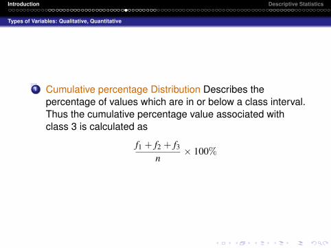
1 Cumulative percentage Distribution Describes thepercentage of values which are in or below a class interval.Thus the cumulative percentage value associated withclass 3 is calculated as
f1 + f2 + f3n
× 100%
Introduction Descriptive Statistics
Types of Variables: Qualitative, Quantitative
Example: Data for Utility Charges
96, 171, 202, 178, 147, 102, 153, 197, 127, 82, ....158
Introduction Descriptive Statistics
Types of Variables: Qualitative, Quantitative
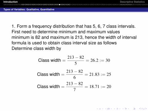
1. Form a frequency distribution that has 5, 6, 7 class intervals.First need to determine minimum and maximum valuesminimum is 82 and maximum is 213, hence the width of intervalformula is used to obtain class interval size as followsDetermine class width by
Class width =213− 82
5= 26.2 := 30
Class width =213− 82
6= 21.83 := 25
Class width =213− 82
7= 18.71 := 20

Introduction Descriptive Statistics
Types of Variables: Qualitative, Quantitative
A chart for 7 intervals
EC Midpoint Freq Per80<100 90 4 8%100<120 110 7 14%120<140 130 9 18%140<160 150 13 26%160<180 170 9 18%180<200 190 5 10%200<220 210 3 6%
Introduction Descriptive Statistics
Types of Variables: Qualitative, Quantitative
Histograms/Polygon graphs
1 Histogram Is a chart in which the rectangular bars areconstructed at the boundaries of each class. When plottinga histogram variable of interest is displayed along the (X)horizontal axis (differentiated by the class boundaries. Thevertical axis(Y) represents the number, proportion orpercentage of observations per class interval.
Introduction Descriptive Statistics
Types of Variables: Qualitative, Quantitative
1 Polygon A percentage Polygon is a line chart, which isuseful for comparing two or more groups. The advantageover a histogram is that it is easier to see visually thedifference between two groups. The percentage polygon isconstructed by connecting lines between the midpoints ofeach interval at their respective class percentages.
Introduction Descriptive Statistics
Types of Variables: Qualitative, Quantitative
1 Cumulative percentage Polygons or Ogives A cumulativepercentage polygon, otherwise known as an Ogive, is aline graph of the cumulative percentage distribution.Similar to the Polygon line chart, it is constructed byconnecting lines between the midpoints of each interval attheir respective cumulative percentages.For example in the case of 7 classes one would construct aplot based on the pairs (70, 0), (90, 8), (110, 22), (130,40),(150,66), (170, 84), (190, 94), (210, 100). Where the firstvalue represents the class midpoints and the second valueis the cumulative percentage up to an including that class.
Introduction Descriptive Statistics
Types of Variables: Qualitative, Quantitative
Scatter Diagram
The scatter diagram is a graphical method used to compare thepossible relationships between two variables of interest.Variable 1 is plotted on the X-axis and variable two on theY-axis. If there are n associated pairs of data then these can berepresented as (X1, Y1), . . . , (Xn, Yn). A question to ask is if thegraphs seem to visually imply a solid relationship between twovariables. A common use of scatter diagrams is to determine ifthere is a linear relationship between the X variable and the Yvariable.

Introduction Descriptive Statistics
Types of Variables: Qualitative, Quantitative
Scatter Diagram _ Oldfaithfuldata
Introduction Descriptive Statistics
Tables and Charts for Categorical Data:
Tables and charts are often used for Categorical data. Thereare many similarities between the methods for numerical dataand categorical data. One main distinction is that the terms,
classes or class intervals, which are based on a range ofnumerical values is replaced by types of objects orcategories.The idea of frequencies or percentages is then taken withrespect to these categories.

Introduction Descriptive Statistics
Tables and Charts for Categorical Data:
Summary Table
The Summary Table is quite similar to the frequency distributiontable for numerical values except that now frequencies andpercentages are calculated with respect to types or categoriesof objects.
Introduction Descriptive Statistics
Tables and Charts for Categorical Data:
Suppose that there are 4 categories labeled {A,B,C,D}, thenone would calculate the number of objects of type A, B, C, D toobtain the frequencies and organize this in a chart.That is, the frequency of A, can be represented as
fA = # of observations in class A
Introduction Descriptive Statistics
Tables and Charts for Categorical Data:
Bar Chart
A Bar Chart is very similar to a histogram. A frequency barchart is constructed by representing each category as a bar,where the length or height of the bar represents the frequencyor percentage of observations falling in that category.

Introduction Descriptive Statistics
Tables and Charts for Categorical Data:
Example: One plots (A, fA), (B, fB), (C, fC) etc, where A, B, Cplay a similar role to the class intervals in a histogram. Notethat unlike histograms there is no real concept of a midpoint.However because the types are represented by equally widebars, one still has a visual midpoint.

Introduction Descriptive Statistics
Tables and Charts for Categorical Data:
Pie Chart
This is a popular graphical device which simply represents thepercentage in each category as pieces of a pie. Hence thecategory with the largest piece of pie, represents the categorywith the largest percentage and so on. In order to properlycalculate the pie chart one uses the formula360× percentage in category.

Introduction Descriptive Statistics
Tables and Charts for Categorical Data:
Pareto Diagram
In many respects a Pareto Diagram is quite similar to an Ogivefor numerical data combined with a Bar chart. To construct onedisplays a ranked Bar chart in decreasing order. That is, the barchart starts with the category with the highest frequency orpercentage then the next highest etc. A cumulative frequencypolygon or Ogive can then be constructed using the visualmidpoints of the bar chart. The ranked bar chart combined withthe overlayed Ogive define the Pareto Diagram.The Pareto Diagram is preferred to the bar chart and pie chartwhen there are many categories.
Introduction Descriptive Statistics
Tables and Charts for Categorical Data:
Tabulating Bivariate Categorical Data
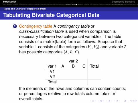
1 Contingency table A contingency table orclass-classification table is used when comparison isnecessary between two categorical variables. The tableconsists of a matrix(table) form as follows: Suppose thatvariable 1 consists of the categories (V1, V2) and variable 2has possible categories (A, B, C)
var 2var 1 A B C TotalV1V2
Total
the elements of the rows and columns can contain counts,or percentages relative to row totals column totals oroverall totals.
Introduction Descriptive Statistics
Tables and Charts for Categorical Data:
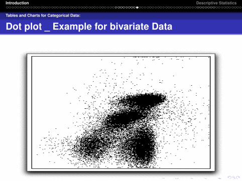
Dot plot _ Example for bivariate Data
Introduction Descriptive Statistics
Numerical Descriptive Measures
Measures of central tendency
Measures of central tendency or location of the data are usedto identify a typical value that can be used to describe the entireset. Three common measurements are the arithmetic mean,median, and the mode. Respectively these measure, theaverage value, the middlemost value, and the most occurringvalue in a dataset.

Introduction Descriptive Statistics
Numerical Descriptive Measures
The Arithmetic Mean
Certainly the most commonly recognized and used measure ofcentral tendency is the arithmetic mean or the (common)average. If a dataset consists of n observations, X1, X2, . . . , Xn,then the arithmetic mean of the sample is written as
X̄ =X1 + X2 + . . . + Xn
n
The sum or total can be expressed in shorthand as,
n∑i=1
Xi := X1 + X2 + . . . + Xn
Introduction Descriptive Statistics
Numerical Descriptive Measures
The mean is often a fine measurement of central tendency.However its main drawback is that it is greatly affected byextreme values in the data.That is values which are much smaller or much larger thanmost of the values in the data set.

Introduction Descriptive Statistics
Numerical Descriptive Measures
Example: Imagine that one wants to find the average income inHong Kong. Average in this sense means one wants to be ableto pinpoint what salary per month the average person makes.In order to do this a survey is taken say based on 10 people atrandom, the people report monthly incomes of4000, 10,000, 10,000, 15,000, 20,000, 25,000, 30,000, 60,000,60,000, 5,000,000 (a BIG TYCOON)The total is 5,226,000 and the average income is
X̄ = 522, 600.
Introduction Descriptive Statistics
Numerical Descriptive Measures
Naturally as n increases this number will most likely decreasebut this example illustrates how sensitive mean calculations canbe.
Introduction Descriptive Statistics
Numerical Descriptive Measures
Median
The Median is the middle value in an ordered array of data. Themedian is not affected by extreme values and may bepreferable to the mean in this situation.There are two methods of computing the median of the set ofdata depending on whether the sample size is even or odd.First one needs to remember to order the data from theminimum to maximum value.
1 When n is odd;
Median =n + 1
2ranked observation
Introduction Descriptive Statistics
Numerical Descriptive Measures
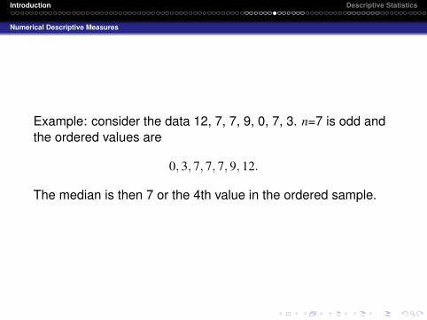
Example: consider the data 12, 7, 7, 9, 0, 7, 3. n=7 is odd andthe ordered values are
0, 3, 7, 7, 7, 9, 12.
The median is then 7 or the 4th value in the ordered sample.

Introduction Descriptive Statistics
Numerical Descriptive Measures
When n is even. The median is defined to be the average of thetwo middle most values.Example: recall the income example. 4000, 10,000, 10,000,15,000, 20,000, 25,000, 30,000, 60,000, 60,000, 5,000,000.The two middlemost values are 20,000 and 25,000 which yieldsa median of
20, 000 + 25, 0002
= 22, 500

Introduction Descriptive Statistics
Numerical Descriptive Measures
1 The Mode The mode corresponds to the value in the dataset which occurs most often.

Introduction Descriptive Statistics
Numerical Descriptive Measures
Geometric Mean:Investments
The Geometric Mean and the Geometric Rate of Return areused to measure the status of an investment over time.Measures the rate of change of a variable over time.
1 The formula for the geometric mean of variables X1, . . . , Xn
isX̄G = (X1 × X2 × · · · × Xn)
1n
2 The formula for the Geometric mean rate of return is
R̄G = [(1 + R1)× · · · × (1 + Rn)]1n − 1
where Ri is the rate of return in time period i. The rate ofreturn is defined to be the loss or gain in period i divided bythe starting value in the period and then multiplied by100%.
Introduction Descriptive Statistics
Numerical Descriptive Measures
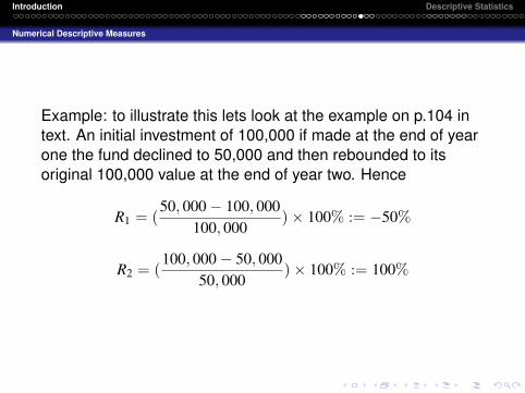
Example: to illustrate this lets look at the example on p.104 intext. An initial investment of 100,000 if made at the end of yearone the fund declined to 50,000 and then rebounded to itsoriginal 100,000 value at the end of year two. Hence
R1 = (50, 000− 100, 000
100, 000)× 100% := −50%
R2 = (100, 000− 50, 000
50, 000)× 100% := 100%
Introduction Descriptive Statistics
Numerical Descriptive Measures
The average return is calculated to be 25,000,
[R1 + R2]/2× 100, 000 = .25× 100, 000
Introduction Descriptive Statistics
Numerical Descriptive Measures
while the geometric mean rate of return is calculated to be
(.5× 2)1/2 − 1 = 0,
which more accurately reflects the fact that at the end of the 2year period there was no gain or loss.

Introduction Descriptive Statistics
Measures of noncentral tendency
Quartiles
The Quartiles divide the ranked data into four quarters.1 The value of the data where 25% of the data is below and
75% are above it is called the 1st quartile, denoted as Q1.A formula for Q1 is given as
Q1 =n + 1
4ordered observation
2 The value of the data where 75% of the data is below and25% are above it is called the 3rd quartile, denoted as Q3.A formula for Q3 is given as
Q1 =3(n + 1)
4ordered observation

Introduction Descriptive Statistics
Measures of noncentral tendency
Example: for the dataset 4000, 10,000, 10,000, 15,000, 20,000,25,000, 30,000, 60,000, 60,000, 5,000,000. Using the formulasthe Q1 correspond to the 2.75 ordered value and Q3corresponds to the 8.25 ordered value. It follows that roundingup 2.75 to 3 yields
Q1 = 10, 000
Rounding down 8.25 to 8,
Q3 = 60, 000
Introduction Descriptive Statistics
Measures of Variation
In addition to measurements of central tendency it is importantto identify the amount of Variability or Spread in data. Threesuch measurements are the Range, Interquartile Range andVariance.Example: As a simple motivating example consider the case oftwo data sets {2,2,2,2,2} and {0,1,2,3,4}
1 The arithmetic mean of both sets is 2 and the median ofboth sets is also 2.
2 However the data sets are quite different. For the first dataset all measures of variation would yield the value 0 whilethis will not be the case for the second data set.
Introduction Descriptive Statistics
Measures of Variation
Range
1 The Range is simply the difference between the minimumvalue and the maximum value of the data.
2 That is the formula
Range = Xlargest − Xsmallest
3 It is a measure of the total spread in the data.4 One drawback is that it does not take into account the
other data points besides the minimum and the maximum.5 Another problem is it is highly sensitive to extreme values

Introduction Descriptive Statistics
Measures of Variation
1 For the simple example above the Range of the seconddata set {0, 1, 2, 3, 4} is
4− 0 = 4
as compared to 2− 2 = 0 for the first set {2, 2, 2, 2, 2}.

Introduction Descriptive Statistics
Measures of Variation
Interquartile Range
1 The interquartile range considers the spread in the middle50% of the data and is therefore not influenced by extremevalues
2 The formula is
Interquartile range = Q3 − Q1
Introduction Descriptive Statistics
Measures of Variation
Example: Calculate the Interquartile range for the data sets{2, 2, 2, 2, 2} and {0, 1, 2, 3, 4}
1 Solution: first note that n = 5 and compute the positions forQ1 and Q3
2 Note that,n + 1
4=
64
= 1.5
3 It follows that Q1 corresponds to the second number andQ3 corresponds to the 3(1.5) := 4.5 or the 5th number.
4 hence for {2, 2, 2, 2, 2}, Q1 = Q3 = 2 and the InterquartileRange is 0.
5 For {0, 1, 2, 3, 4}, Q3 = 4 and Q1 = 1, thus the InterquartileRange is 4− 1 = 3
Introduction Descriptive Statistics
Measures of Variation
Variance and Standard Deviation
The Sample Variance of a data set is defined as,
S2 =(X1 − X)2 + · · ·+ (Xn − X)2
n− 1
Introduction Descriptive Statistics
Measures of Variation
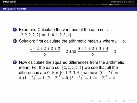
1 Example: Calculate the variance of the data sets{2, 2, 2, 2, 2} and {0, 1, 2, 3, 4}
2 Solution: first calculate the arithmetic mean X where n = 5.
2 + 2 + 2 + 2 + 25
= 2 and0 + 1 + 2 + 3 + 4
5= 2
3 Now calculate the squared differences from the arithmeticmean. For the data set {2, 2, 2, 2, 2} we see that all thedifferences are 0. For {0, 1, 2, 3, 4}, we have (0− 2)2 =4, (1− 2)2 = 1, (2− 2)2 = 0, (3− 2)2 = 1, (4− 2)2 = 4
Introduction Descriptive Statistics
Measures of Variation
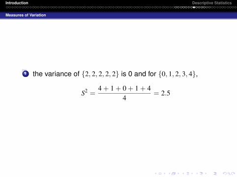
1 the variance of {2, 2, 2, 2, 2} is 0 and for {0, 1, 2, 3, 4},
S2 =4 + 1 + 0 + 1 + 4
4= 2.5
Introduction Descriptive Statistics
Measures of Variation
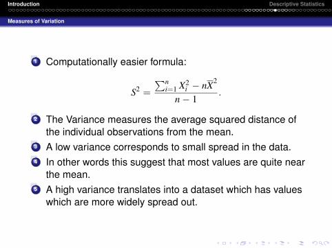
1 Computationally easier formula:
S2 =∑n
i=1 X2i − nX2
n− 1.
2 The Variance measures the average squared distance ofthe individual observations from the mean.
3 A low variance corresponds to small spread in the data.4 In other words this suggest that most values are quite near
the mean.5 A high variance translates into a dataset which has values
which are more widely spread out.
Introduction Descriptive Statistics
Measures of Variation
Standard Deviation
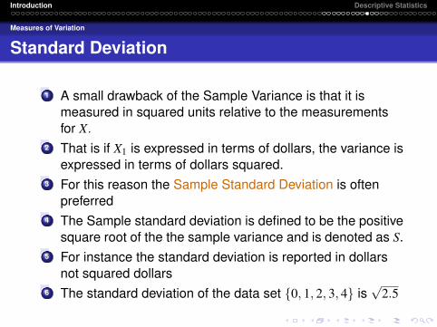
1 A small drawback of the Sample Variance is that it ismeasured in squared units relative to the measurementsfor X.
2 That is if X1 is expressed in terms of dollars, the variance isexpressed in terms of dollars squared.
3 For this reason the Sample Standard Deviation is oftenpreferred
4 The Sample standard deviation is defined to be the positivesquare root of the the sample variance and is denoted as S.
5 For instance the standard deviation is reported in dollarsnot squared dollars
6 The standard deviation of the data set {0, 1, 2, 3, 4} is√
2.5
Introduction Descriptive Statistics
Measures of Variation
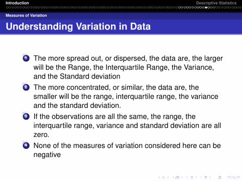
Understanding Variation in Data
1 The more spread out, or dispersed, the data are, the largerwill be the Range, the Interquartile Range, the Variance,and the Standard deviation
2 The more concentrated, or similar, the data are, thesmaller will be the range, interquartile range, the varianceand the standard deviation.
3 If the observations are all the same, the range, theinterquartile range, variance and standard deviation are allzero.
4 None of the measures of variation considered here can benegative
Introduction Descriptive Statistics
Measures of Variation
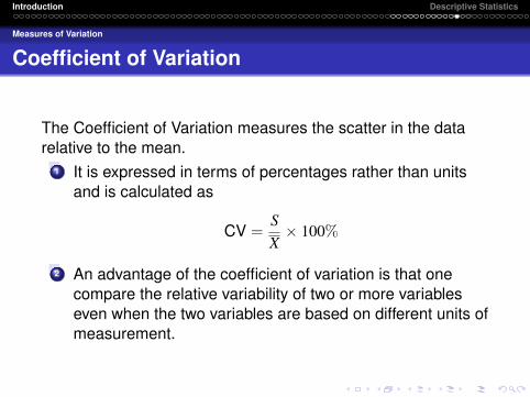
Coefficient of Variation
The Coefficient of Variation measures the scatter in the datarelative to the mean.
1 It is expressed in terms of percentages rather than unitsand is calculated as
CV =SX× 100%
2 An advantage of the coefficient of variation is that onecompare the relative variability of two or more variableseven when the two variables are based on different units ofmeasurement.
Introduction Descriptive Statistics
Shape of a data set
Shape of Data
The third property of a data set is related to the way the dataare distributed. All descriptions of shape are taken relative tohow symmetric the data set is. A data set which is notsymmetric is said to be asymmetrical or skewed

Introduction Descriptive Statistics
Shape of a data set
Symmetrical data set
1 A data set is considered symmetric if the mean andmedian are equal That is, X =Median
2 A data set is right-skewed if the mean is greater than themedian. X >Median In other words there are someextremely large values in the data
3 A data set is left-skewed if the mean is less than themedian. X <Median That is, there are some extremelysmall values in the data

Introduction Descriptive Statistics
Shape of a data set
Question 1
Which of the following is sensitive to extreme values
1. The median2. The Interquartile range3. The arithmetic mean4. the 1st Quartile, Q1
Introduction Descriptive Statistics
Shape of a data set
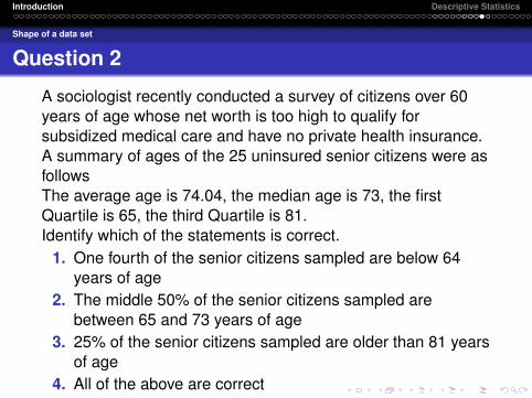
Question 2
A sociologist recently conducted a survey of citizens over 60years of age whose net worth is too high to qualify forsubsidized medical care and have no private health insurance.A summary of ages of the 25 uninsured senior citizens were asfollowsThe average age is 74.04, the median age is 73, the firstQuartile is 65, the third Quartile is 81.Identify which of the statements is correct.
1. One fourth of the senior citizens sampled are below 64years of age
2. The middle 50% of the senior citizens sampled arebetween 65 and 73 years of age
3. 25% of the senior citizens sampled are older than 81 yearsof age
4. All of the above are correct

Introduction Descriptive Statistics
Shape of a data set
Example: Sample: {5, 7, 1, 2, 4}
Xi (Xi − X) (Xi − X)2 Xi2
5 1.2 1.44 257 3.2 10.24 491 -2.8 7.84 12 -1.8 3.24 44 0.2 0.04 16
sum 19 0 22.8 95
X =195
= 3.8
S2 =22.8
4= 5.7 and S = 2.387
CV =SX
= 62.8%

Introduction Descriptive Statistics
Describing Central Tendency
Some measures of central tendency for numericaldata
Population (N objects) vs Sample (n objects) // Parametervs. StatisticThe sample mean x̄ is a point estimate of the populationmean µ
x̄ =x1 + x2 + . . . + xn
n=
1n
n∑i=1
xi
The Median Md is the middlemost measurement in theordering
Introduction Descriptive Statistics
Describing Central Tendency
if n = 2p + 1 is odd: it is the (p + 1)th.if n = 2p is even: it is the average of the pth and (p + 1)th
The Mode M0 is the measurement that occurs mostfrequently.
Introduction Descriptive Statistics
Measure of Variation
Some measures of variation for numerical data
The Range is the largest measurement minus the smallestmeasurementThe sample VarianceStandard Deviation
Introduction Descriptive Statistics
Percentiles, Quartiles, and Box-and-Whiskers Displays
Questions
1. For each of the following random variables, determinewhether the variable is categorical or numerical(quantitative).
a) Number of telephones per householdb) Type of telephone primarily usedc) Number of long-distance calls made per monthd) Length (in minutes) of longest long-distance call made per
monthe) Color of telephone primarily usedf) monthly charge (in dollars and cents) for long distance
calls madeg) ownership of a cellular phone
Introduction Descriptive Statistics
Summarizing Data/Exploratory data Analysis
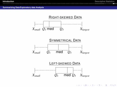
1 5-number summary provides a way of determining theshape of data based on the quantities
Xsmallest Q1 median Q3 Xlargest
2 Box and Whisker plots: Uses the 5-number summary tographically represent the data.
Introduction Descriptive Statistics
Summarizing Data/Exploratory data Analysis
Xsmall Q1 med Q3 Xlargest
LEFT-SKEWED DATA
Xsmall Q1 med Q3 Xlargest
SYMMETRICAL DATA
Xsmall Q1 med Q3 Xlargest
RIGHT-SKEWED DATA
Introduction Descriptive Statistics
Summarizing Data/Exploratory data Analysis
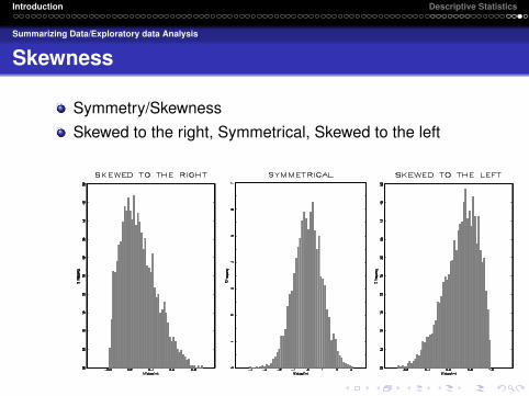
Skewness
Symmetry/SkewnessSkewed to the right, Symmetrical, Skewed to the left

Introduction Descriptive Statistics
Descriptive measures of the Population
Suppose that X1, . . . , XN represents now all possible valuesfrom a population of size N.
1 Note that in some cases the population size N may beunknown or infinite. An example of a finite population is thecollection of students at UST.
2 Similar to the arithmetic mean of the sample, we cancalculate the true mean of the population, denoted as µ.
µ =∑N
i=1 Xi
N3 The variance of the Population is calculated as Population
variance σ2 and Population standard deviation σ of dataX1, X2, . . . , XN :
σ2 =1N
N∑i=1
(Xi − µ)2 and σ =√
σ2
Introduction Descriptive Statistics
Descriptive measures of the Population
The phrase within k standard deviations from the mean refersto data which are in an interval
[µ− kσ, µ + kσ]
Introduction Descriptive Statistics
Descriptive measures of the Population
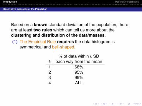
Based on a known standard deviation of the population, thereare at least two rules which can tell us more about theclustering and distribution of the data/masses.(1) The Empirical Rule requires the data histogram is
symmetrical and bell-shaped.
% of data within k SDk each way from the mean1 68%2 95%3 99%4 ALL
Introduction Descriptive Statistics
Descriptive measures of the Population
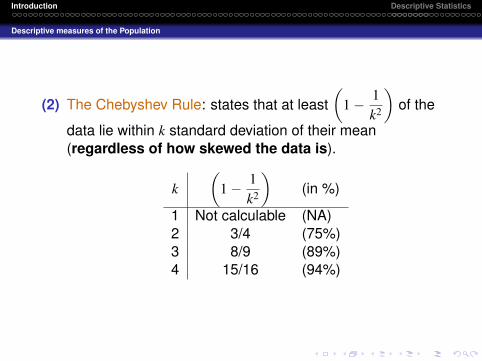
(2) The Chebyshev Rule: states that at least(
1− 1k2
)of the
data lie within k standard deviation of their mean(regardless of how skewed the data is).
k(
1− 1k2
)(in %)
1 Not calculable (NA)2 3/4 (75%)3 8/9 (89%)4 15/16 (94%)
Introduction Descriptive Statistics
Descriptive measures of the Population
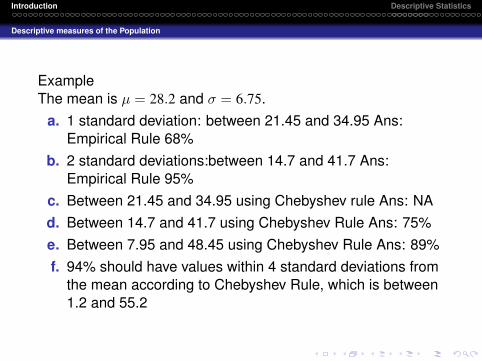
ExampleThe mean is µ = 28.2 and σ = 6.75.
a. 1 standard deviation: between 21.45 and 34.95 Ans:Empirical Rule 68%
b. 2 standard deviations:between 14.7 and 41.7 Ans:Empirical Rule 95%
c. Between 21.45 and 34.95 using Chebyshev rule Ans: NAd. Between 14.7 and 41.7 using Chebyshev Rule Ans: 75%e. Between 7.95 and 48.45 using Chebyshev Rule Ans: 89%f. 94% should have values within 4 standard deviations from
the mean according to Chebyshev Rule, which is between1.2 and 55.2
Introduction Descriptive Statistics
Descriptive measures of the Population
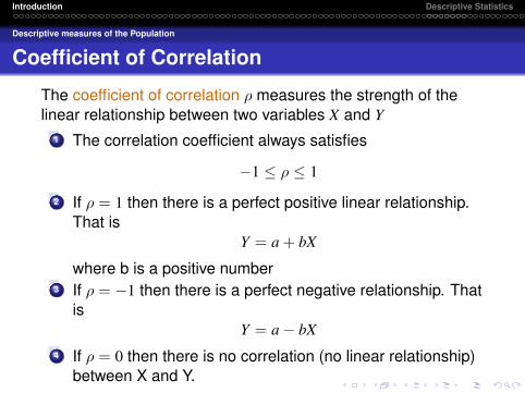
Coefficient of Correlation
The coefficient of correlation ρ measures the strength of thelinear relationship between two variables X and Y
1 The correlation coefficient always satisfies
−1 ≤ ρ ≤ 1
2 If ρ = 1 then there is a perfect positive linear relationship.That is
Y = a + bX
where b is a positive number3 If ρ = −1 then there is a perfect negative relationship. That
isY = a− bX
4 If ρ = 0 then there is no correlation (no linear relationship)between X and Y.
Introduction Descriptive Statistics
Descriptive measures of the Population
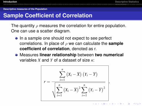
Sample Coefficient of Correlation
The quantity ρ measures the correlation for entire population.One can use a scatter diagram.
In a sample one should not expect to see perfectcorrelations. In place of ρ we can calculate the samplecoefficient of correlation, denoted as r.Measures linear relationship between two numericalvariables X and Y of a dataset of size n:
r =
n∑i=1
(Xi − X
) (Yi − Y
)√√√√ n∑
i=1
(Xi − X
)2n∑
i=1
(Yi − Y
)2
,

Introduction Descriptive Statistics
Descriptive measures of the Population
where −1 ≤ r ≤ 1 .
Introduction Descriptive Statistics
Descriptive measures of the Population
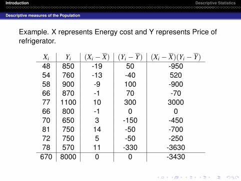
Example. X represents Energy cost and Y represents Price ofrefrigerator.
Xi Yi (Xi − X) (Yi − Y) (Xi − X)(Yi − Y)48 850 -19 50 -95054 760 -13 -40 52058 900 -9 100 -90066 870 -1 70 -7077 1100 10 300 300066 800 -1 0 070 650 3 -150 -45081 750 14 -50 -70072 750 5 -50 -25078 570 11 -330 -3630
670 8000 0 0 -3430
Introduction Descriptive Statistics
Descriptive measures of the Population
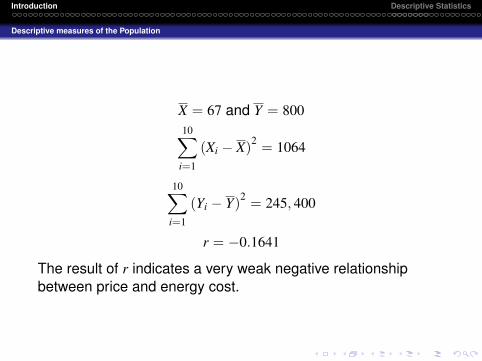
X = 67 and Y = 80010∑
i=1
(Xi − X)2 = 1064
10∑i=1
(Yi − Y)2 = 245, 400
r = −0.1641
The result of r indicates a very weak negative relationshipbetween price and energy cost.


