Lectures 10 and 11: Principal Component Analysis (PCA) and Independent Component Analysis(ICA) Objectives: Both PCA and ICA are used to reduce measured data into a smaller set of components. PCA - utilizes the first and second moments of the measured data, hence relying heavily on Gaussian features ICA - exploits inherently non-Gaussian features of the data and employs higher moments FastICA website: http://www.cis.hut.fi/projects/ica/fastica/
Transcript
Lectures 10 and 11:Principal Component Analysis (PCA) and
Independent Component Analysis(ICA)
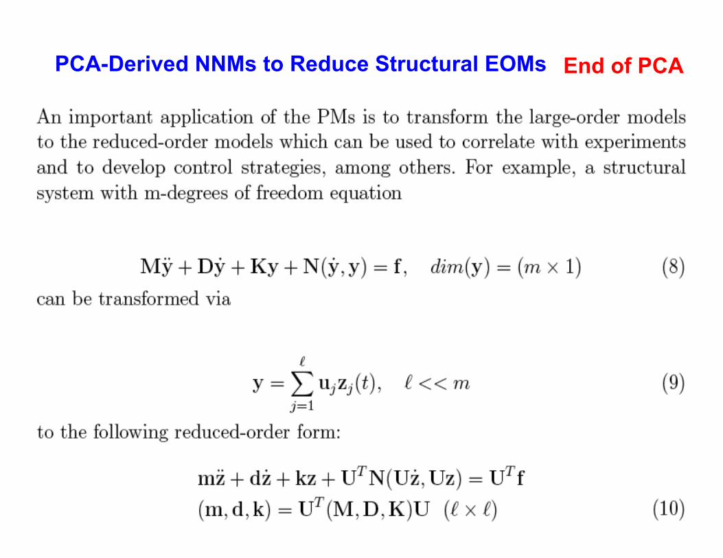
Objectives: Both PCA and ICA are used to reduce measured data into a smaller set of components.
PCA - utilizes the first and second moments of the measured data, hence relying heavily on Gaussian features
ICA - exploits inherently non-Gaussian features of the data and employs higher moments
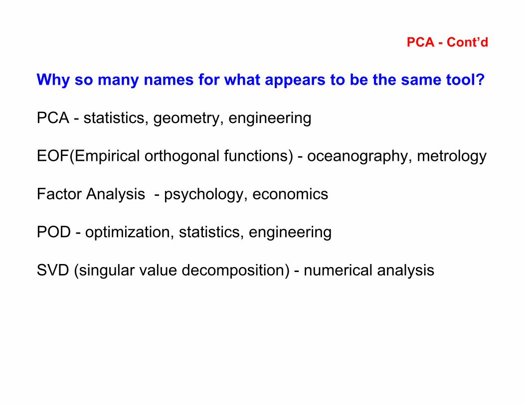
SVD (singular value decomposition) - numerical analysis
PCA - Cont’dA little dig into its mathematics
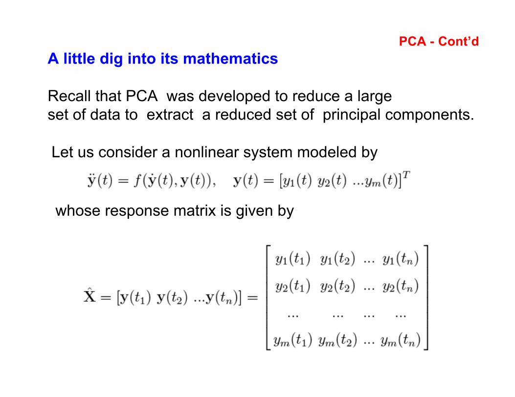
Recall that PCA was developed to reduce a large set of data to extract a reduced set of principal components.
Let us consider a nonlinear system modeled by
whose response matrix is given by
PCA - Cont’d A little dig into its mathematics
If the mean values of each of the row vector are not zero,we modify the previous X to read
where is the mean value of the response data.
PCA - Cont’dA little dig into its mathematics
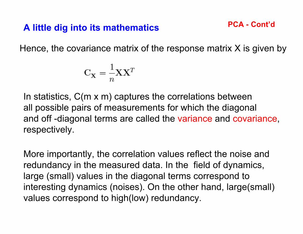
Hence, the covariance matrix of the response matrix X is given by
In statistics, C(m x m) captures the correlations between all possible pairs of measurements for which the diagonal and off -diagonal terms are called the variance and covariance, respectively.
More importantly, the correlation values reflect the noise and redundancy in the measured data. In the field of dynamics, large (small) values in the diagonal terms correspond to interesting dynamics (noises). On the other hand, large(small) values correspond to high(low) redundancy.
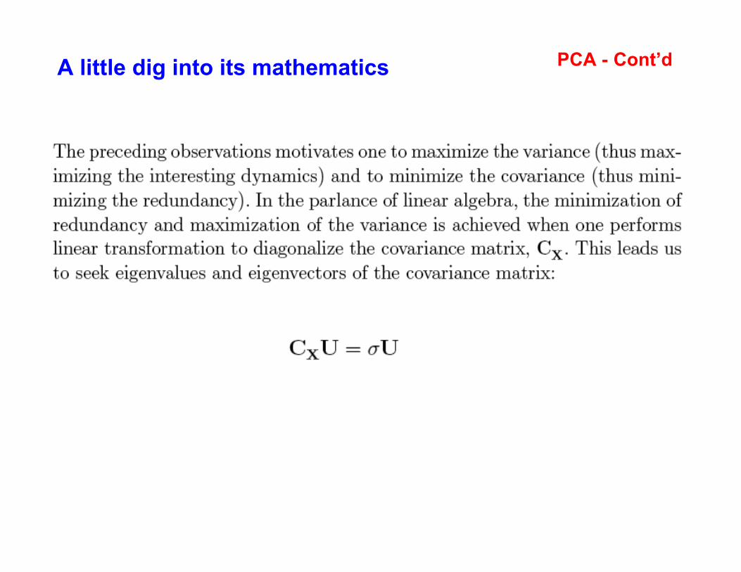
PCA - Cont’dA little dig into its mathematics
Some Remarks on PCA
PCA-Derived NNMs to Reduce Structural EOMs End of PCA
Independent component analysis (ICA)
PCA (Principal Component Analysis) seems to cover awide range of data analysis; in addition, for transient datawe have Hilbert-Huang Transform.
So why do we need ICA?
PCA is based on the second-order statistics. That is,data fit Gaussian distribution (i.e., exploit correlation/covariance properties)
What if data cannot be characterized by the secondmoment? That is, Rx = E{xxT} = I (white noise)?
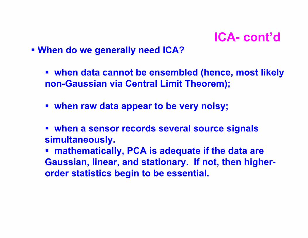
ICA- cont’d When do we generally need ICA?
when data cannot be ensembled (hence, most likelynon-Gaussian via Central Limit Theorem);
when raw data appear to be very noisy;
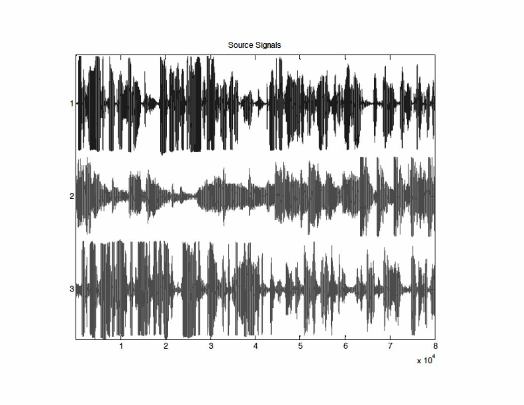
when a sensor records several source signalssimultaneously. mathematically, PCA is adequate if the data areGaussian, linear, and stationary. If not, then higher-order statistics begin to be essential.
Comparison of PCA with ICA
PCA minimizes the covariance of the data; on the other hand ICA minimizes higher-order statistics such as fourth-order cummulant (or kurtosis), thus minimizing the mutual information of the output.
Specifically, PCA yields orthogonal vectors of high energy contents in terms of the variance of the signals, whereasICA identifies independent components for non-Gaussian signals.
ICA thus possesses two ambiguities:
First, the ICA model equation is underdetermined system; one cannot determine the variances of the independent components.
Second, one cannot rank the order of dominant components.
Historically there is a good reason why ICA came to be studied only recently, whereas random variables are assumed to be Gaussian in most of statistical theory;
ICA thrives on the fact that the data are non-Gaussian.
This implies that ICA exploits the loose end of the Central Limit Theorem which states that the distribution of a sum of independent random variables tends toward a Gaussian distribution. Fortunately for ICA, there are many cases wheresome real-world data do not have sufficient data pools that can be characterized as Gaussian.
Why ICA has been a late bloomer
ICA- cont’dICA in a nutshell
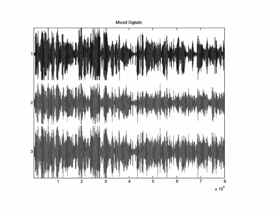
Given measurement, x, find the independentcomponents, s, and the associated mixing matrix, A,such that x = As
Find wj that maximizes non-Gaussianity of wjTx
Independent components s is then found from
s = W x where A-1 = W = [w1 w2 … wm]
Fast ICA in words
A Fast ICA Algorithm (using Negentropy concept)
1. Center the data, x, to make its mean zero (same as PCA): x <= x - xm, xm = E{x}
2. Whiten x to maximize non-Gaussian characteristics(PCAwith filtering):
z = V Λ−1/2 VT x, V Λ VT = E{xxT}
3. Choose an initial random vector, w, ||w|| =1
4. Update w (maximally non-Gaussian direction!) w = E{z * g(wT z)} - E{g ��’ (wT z)}w, g(y) = tanh(a1y) or y*exp(-y2/2), 1<a1 <2 w = w/||w||
5. If not converged, then go back to step 4.
6. Obtain the independent component, s:
7. s = [ w1 w2 … wn ] x
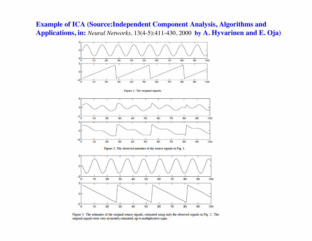
Example of ICA (Source:Independent Component Analysis, Algorithms andApplications, in: Neural Networks, 13(4-5):411-430, 2000 by A. Hyvarinen and E. Oja)
ICA for Nonlinear Problems? Source: http://videolectures.net/mlss05au_hyvarinen_ica/
Nonlinear is nonparametric? Usually, this means very general functions: x=f(s) where f is “almost anything”
Should perhaps be called nonparametric as in statistics Can this be solved for a general f(s)? No.
Indeterminacy of nonlinear ICA We can always find an infinity of different nonlinear functions g so that y=g(x) has independent components and these are very different solutions from each other;
We must restrict the problem in some way;
Recently, many people propose xi = f( wi
t x)where f is scalar. “Post-nonlinear” mixtures
Nonlinear ICA
A simple solution? Do nonlinear PCA
(e.g. Kohonen map) and then linear ICA (very constrained)
Another solution: constrain the nonlinearity to besmooth, use this as Bayesian prior (Harri Valpolaet al)