89
Lectures in Open Economy Macroeconomics Mart´ ın Uribe 1 This draft, March 8, 2005 1 Duke University. E-mail: [email protected].

Lectures in Open Economy Macroeconomics
Martın Uribe1
This draft, March 8, 2005
1Duke University. E-mail: [email protected].

ii

Contents
1 The Current Account in an Endowment Economy 11.1 The Model Economy . . . . . . . . . . . . . . . . . . . . . . . 11.2 Response of the Current Account to Output Shocks . . . . . 41.3 Current Account Dynamics With Nonstationary Income Shocks 51.4 Empirical Evaluation of the Endowment Economy . . . . . . 71.5 Other Tests of the Model . . . . . . . . . . . . . . . . . . . . 10
2 The Current Account in an Economy with Capital 172.1 No Capital Adjustment Costs . . . . . . . . . . . . . . . . . . 17
2.1.1 A Permanent Productivity Shock . . . . . . . . . . . . 192.1.2 A Temporary Productivity shock . . . . . . . . . . . . 20
2.2 Capital Adjustment Costs . . . . . . . . . . . . . . . . . . . . 212.2.1 Dynamics of the capital stock . . . . . . . . . . . . . . 222.2.2 A Permanent Technology Shock . . . . . . . . . . . . . 24
3 The Current Account in a Real-Business-Cycle Model 273.1 The Model (Model 1) . . . . . . . . . . . . . . . . . . . . . . 273.2 The Model’s Performance . . . . . . . . . . . . . . . . . . . . 323.3 Alternative Ways To Close The Small Open Economy Model 35
3.3.1 Endogenous Discount Factor Without Internalization(Model 1a) . . . . . . . . . . . . . . . . . . . . . . . . 38
3.3.2 Debt Elastic Interest Rate (Model 2) . . . . . . . . . 393.3.3 Portfolio Adjustment Costs (Model 3) . . . . . . . . . 403.3.4 Complete Asset Markets (Model4) . . . . . . . . . . . 413.3.5 The Nonstationary Case (Model 5) . . . . . . . . . . . 433.3.6 Quantitative Results . . . . . . . . . . . . . . . . . . . 44
3.4 Appendix . . . . . . . . . . . . . . . . . . . . . . . . . . . . . 463.4.1 Log-Linearization of the Equilibrium Conditions . . . 46
3.5 Exercise . . . . . . . . . . . . . . . . . . . . . . . . . . . . . . 46
iii

iv CONTENTS
4 Solving Dynamic General Equilibrium Models By LinearApproximation 514.1 The Schur Decomposition Method . . . . . . . . . . . . . . . 53
4.1.1 Matlab Code . . . . . . . . . . . . . . . . . . . . . . . 554.2 Computing Second Moments . . . . . . . . . . . . . . . . . . 56
4.2.1 Method 1 . . . . . . . . . . . . . . . . . . . . . . . . . 564.2.2 Method 2 . . . . . . . . . . . . . . . . . . . . . . . . . 574.2.3 Method 3 . . . . . . . . . . . . . . . . . . . . . . . . . 574.2.4 Other second moments . . . . . . . . . . . . . . . . . . 57
4.3 Impulse Response Functions . . . . . . . . . . . . . . . . . . . 584.4 Higher Order Approximations . . . . . . . . . . . . . . . . . . 58
5 Business Cycles In Emerging Economies (In Progress) 615.1 Some Empirical Regularities . . . . . . . . . . . . . . . . . . . 615.2 Trends and Cycles . . . . . . . . . . . . . . . . . . . . . . . . 63
5.2.1 A Small Open Economy With Nonstationary Shocks . 645.2.2 Equilibrium . . . . . . . . . . . . . . . . . . . . . . . . 65
6 Exchange-Rate-Based Inflation Stabilization 676.0.3 Market-clearing conditions . . . . . . . . . . . . . . . . 71
7 Models of Balance of Payments Crises 737.1 The Krugman Model . . . . . . . . . . . . . . . . . . . . . . . 73
7.1.1 PPP and Uncovered Interest Parity Condition . . . . 747.1.2 The government . . . . . . . . . . . . . . . . . . . . . 747.1.3 The Monetary/Fiscal Regime . . . . . . . . . . . . . . 747.1.4 A Balance-of-Payments (BOP) Crisis . . . . . . . . . . 757.1.5 Computing T . . . . . . . . . . . . . . . . . . . . . . . 76

List of Tables
1.1 Parameter Estimates of the VAR system . . . . . . . . . . . . 14
3.1 Calibration of the Samll Open RBC Economy . . . . . . . . . 303.2 Business-cycle properties: Data and Model . . . . . . . . . . 333.3 Model 2: Calibration of Parameters Not Shared With Model 1 403.4 Observed and Implied Second Moments . . . . . . . . . . . . 48
5.1 Business Cycles in Argentina and Canada . . . . . . . . . . . 625.2 Business Cycles: Emerging Vs. Developed Economies . . . . 63
v

vi LIST OF TABLES

List of Figures
1.1 Impulse Response To An Output Shock . . . . . . . . . . . . 15
2.1 The Dynamics of the Capital Stock . . . . . . . . . . . . . . . 23
3.1 Small Open Economy RBC Model: Impulse Responses to aPositive Technology Shock . . . . . . . . . . . . . . . . . . . . 34
3.2 Small Open Economy RBC Model: Response of the TradeBalance To a Positive Technology Shock Under AlternativeParameterizations . . . . . . . . . . . . . . . . . . . . . . . . 35
3.3 Impulse Response to a Unit Technology Shock in Models 1 - 5 49
vii

viii LIST OF FIGURES

Chapter 1
The Current Account in anEndowment Economy
The purpose of this chapter is to build a canonical dynamic, general equi-librium model of the open economy capable of capturing a number of basicempirical regularities associated with the current account and other macro-economic variables of interest.
1.1 The Model Economy
Consider an economy populated by a large number of infinitely lived house-holds with preferences described by the utility function
E0
∞∑
t=0
βtU(ct), (1.1)
where ct denotes consumption of the single, perishable good available in theeconomy, and U denotes the single-period utility function, which is assumedto be strictly increasing and strictly concave.
The evolution of the debt position of the representative household isgiven by
dt = (1 + r)dt−1 + ct − yt. (1.2)
where dt denotes the debt position chosen in period t, r denotes the in-terest rate, assumed to be constant, and yt is an exogenous and stochasticendowment of goods. The endowment process represents the sole source ofuncertainty in this economy. The above constr4aint states that the changein the level of debt, dt−dt−1, has two sources, interest services on previously
1

2 Martın Uribe
acquired debt, rdt−1, and excess expenditure over income, ct − yt. House-holds are subject to the following borrowing constraint that prevents themfrom engaging in Ponzi games:
limj→∞
Etdt+j
(1 + r)j≤ 0. (1.3)
This limit conditions says that the household’s debt position must grow ata rate lower than the interest rate r. The optimal allocation of debt willalways feature this constraint holding with strict equality. This is because ifthe allocation {ct, dt}∞t=0 satisfies the no-Ponzi-game constraint with strictinequality, then one can choose an alternative allocation {c′t, d′t}∞t=0 that alsosatisfies the no-Ponzi-game constraint and satisfies c′t ≥ ct, with c′t′ > ct′
for at least one date t′ ≥ 0. This alternative allocation is clearly strictlyprefer to the original one because the single period utility function is strictlyincreasing. The household chooses sequences for ct, and dt for t ≥ 0, so asto maximize (1.1) subject to (1.2) and (1.3). The optimality conditionsassociated with this problem are (1.2), (1.3) holding with equality, and thefollowing Euler condition:
U ′(ct) = β(1 + r)EtU ′(ct+1). (1.4)
The interpretation of this expression is simple. If the household sacrificesone unit of consumption in period t and invests it in financial assets, itsperiod-t utility falls by U ′(ct). In period t + 1 the household receives theunit of goods invested plus interests, 1 + r, yielding β(1 + r)U ′(ct+1) utils.At the optimal allocation, the cost and benefit must equal each other.
We make two additional assumptions that greatly facilitates the analysis.First we require that the subjective and pecuniary rates of discount, β and1/(1 + r) are equal to each other, that is,
β(1 + r) = 1.
This assumption elininates long-run growth in consumption. Second, weassume that the period utility index is quadratic and given by
U(c) = −12(c− c)2, (1.5)
with c < c.1 This particular functional form makes it possible to obtaina closed-form solution of the model. Under these assumptions, the Euler
1You should recognize these as the assumptions of the Hall (1978) permanent incomemodel of consumption.

Lectures in Open Economy Macroeconomics, Chapter 1 3
condition (1.4) collapses toct = Etct+1, (1.6)
which says that consumption follows a random walk.We will now use the household’s sequential budget constraint (1.2) and
the no-Ponzi-scheme constriant (1.3) holding with equality—also known asthe transversality condition—to derive an intertemporal resource constraint.Begin by expressing the sequential budget constraint in period t as
(1 + r)dt−1 = dt + yt − ct
Lead this equation 1 period and use it to get rid of dt:
(1 + r)dt−1 = yt − ct +yt+1 − ct+1
1 + r+
dt+1
1 + r
Repeat this procedure s times to get
(1 + r)dt−1 =s∑
j=0
yt+j − ct+j(1 + r)j
+dt+s
(1 + r)s
Apply expectations conditional on information available at time zero andtake the limit for s → ∞ using the transversality condition (equation (1.3)holding with equality) to get the following intertemporal resource constraint:
(1 + r)dt−1 = Et
∞∑
j=0
yt+j − ct+j(1 + r)j
.
Intuitively, this equation says that the initial net foreign debt position mustbe equal to the expected present discounted value of current and futuredifferences between output and absorption.
Now use the Euler equation (1.6) to deduce that Etct+j = ct. Using thisresult to get rid of expected future consumption in the above expression andrearrange to obtain
(1 + r)[rdt−1 + ct] = rEt
∞∑
j=0
yt+j(1 + r)j
. (1.7)
To be able to fully characterize the equilibrium in this economy, we assumethat the endowment process follows an AR(1) process of the form,
yt = ρyt−1 + εt

4 Martın Uribe
Then, the j-period ahead forecast of output in period t is given by
Etyt+j = ρjyt.
Using this expression to eliminate expectations of future income from equa-tion (1.7), we obtain
(1 + r)[rdt−1 + ct] = ytr
∞∑
j=0
(ρ
(1 + r)
)j
= ytr1 + r
1 + r − ρ
Solving for ct, we obtain
ct =r
1 + r − ρyt − rdt−1
according to this expression, households spend each period the annuity as-sociated with their endowment stream. Part of this income they allocateto consumption and the rest to serve their financial oblitations. Lettingtbt ≡ y − ct and cat ≡ −rdt−1 + tbt denote, respectively, the trade balanceand the current account in period t, we have
tbt = rdt−1 +1 − ρ
1 + r − ρyt
cat =1 − ρ
1 + r − ρyt
1.2 Response of the Current Account to Output
Shocks
Assume that 0 < ρ < 1, so that endowment shocks are positively seriallycorrelated, and consider the response of our model economy to an unantici-pated endowment shock. Two polar cases are of particular interest. In thefirst case, the endowment shock is assumed to be purely transitory, ρ = 0.In this case, only a very small fraction, r/(1 + r, of the increase in outputis allocated to current consumption. Most of the endowment increase—afraction 1/(1 + r))—is saved. The intuition for this result is clear. Becausethe shock is temporary, households smooth consumption by eating a tinypart of it today and leaving the rest for future consumption. In this case,the current account plays the role of a shock absorber. Households borrow

Lectures in Open Economy Macroeconomics, Chapter 1 5
to finance negative shocks and save in response to positive shocks. As aresult, the current account is procyclical, improving during expansions anddeteriorating during contractions.
Consider the case of highly persistent shocks, ρ→ 1. In this case, house-holds allocate all of the increase in output to current consumpiton. Thus,the current account is unchanged. Intuitively, if the shock is permanent,the best response is to adjust to the new level of output by increasing orreducing the standard of living according to whether the shock is positiveor negative.
Therefore, in this model, which captures the esence of what has becameknown as the intertemporal approach to the current account, external bor-rowing is conducted under the the principle: ‘finance temporary shocks,adjust to permanent shocks.’
1.3 Current Account Dynamics With Nonstation-ary Income Shocks
The main prediction of the model presented in the previous section is theprocyclicality of the current account-to-output ratio in economies holdinga positive asset position with respect to the rest of the world. As we willsee shortly, this prediction is counterfactual. In most countries the currentaccount is countercyclical. That is, periods of economic expansion are typi-cally characterized by current account deficits, and recessions take place inthe context of current account surpluses in the external account. Here, weexplore a simple modification to the model that gets around its problem-atic prediction. The modification consists in assuming that the the incomeprocess is nonstationary. Istead, we assume stationarity in the growth rateof income. Consider an infinitely lived household with preferences given by
max−12E0
∞∑
0
βt(ct − ct)2.
Note that the satiation point ct, is now time varying. We will say moreabout this variable shortly. As in the model of the previous section, thehousehold’s problem consists in maximazing this utility fucntion subject tothe resource constraint
dt = (1 + r)dt−1 + ct − yt

6 Martın Uribe
Suppose that the endowment process evolves according to the following lawof motion
yt = (1 + µ)(1 + εt)yt−1,
where εt is an i.i.d. shock with mean zero. The parameter µ ≥ 0 denotes themean growth rate of he endowment. The level of income is nonstationary, inthe sense that an output shock produces a permanent increase in the levelof output. The growth rate of output, given by ln(yt/yt−1 ≈ µ + εt, is i.ı...with mean µ.
Let us scale all variables in the model by tthe level of income. Dividingthe resource constraint through by yt−1 we obtain
dt =1 + r
1 + µ
dt−1
1 + εt+ ct − 1,
where a tilde on a variable denotes the ratio of that varialbe to output.Assume that the subsistence level of consumption, ct satisfies ct/yt = c,where c is a pocitive constant. Then we can write the utility functon as
−12E0
∞∑
0
βt(ct − c)2y2t
The first-order conditon of the household’s problem is
(ct − c)y2t = β
1 + r
1 + µEt(ct+1 − c)
y2t+1
1 + εt+1
For convenience, we will assume that the drift parameter is nil. That is,
µ = 0.
Then, imposing the parameter restriction β(1+r) = 1, the above optimalityconditions can be written as
ct − c = Et(ct+1 − c)(1 + εt+1)
Linearizing the resource constraint and this expression around the deter-ministic steady state, we obtain, respectively
∆dt = (∆dt−1 − dεt) + ∆ct
and∆ct = (1 + r)Et∆ct+1.

Lectures in Open Economy Macroeconomics, Chapter 1 7
Solving the first of these equations forward yields
−(1 + r)∆dt−1 = Et
∞∑
j=0
(1 + r)−j[∆ct+j − dεt+j ]
Using the linearized Euler equation and the fact that the income innovationhas mean zero, yields
−(1 + r)∆dt−1 =1 + r
r∆ct − dεt
Solving for consumption, we have that
∆ct = −r∆dt−1 +rd
1 + rεt
Letting tbyt ≡ (yt− ct)/yt ≡ 1− ct denote the trade balance to output ratioin period t, we have that
∆tbyt = r∆dt−1 −rd
1 + rεt
So the trade balance to output ratio deteriorates in response to a positiveinnovation in output growth. The intuition behind this result is as follows:Because the income shock is permanent, consumption increases roughly bythe same amount as income. But if the country is indebted, consumptionmust be less than, as the economy allocates resources to service its externalobligations. Therefore, if consumption and income increase by the sameamount, the percent increase in consumption is larger than the percent in-crease in income. Thus, the trade balance to output ratio falls. An interest-ing testable implication of the simple model analyzed here is that the tradebalance to output ratio should be more countercyclical the more indebted isthe country. Moreover, the model predicts that the trade balance to outputratio must behave procyclicaly in countries holding a positive net foreignasset position.
1.4 Empirical Evaluation of the Endowment Econ-
omy
A key implication of the model economy we are analyzing is that the tradebalance and the current account improve in response to a positive output

8 Martın Uribe
shock. Here we ask the question of whether this prediction is born by thedata. To this end, we consider the predictions of a simple empirical model.
The empirical model we consider is the following VAR system:2
A
ytıttbytRustRt
= B
yt−1
ıt−1
tbyt−1
Rust−1
Rt−1
+
εytεitεtbytεrust
εrt
(1.8)
where yt denotes real gross domestic output, it denotes real gross domesticinvestment, tbyt denotes the trade balance to output ratio, Rust denotes thegross real US interest rate, and Rt denotes the gross real (emerging) countryinterest rate. A hat on top of yt and it denotes log deviations from a log-linear trend. A hat on Rust and Rt denotes simply the log. We measureRust as the 3-month gross Treasury bill rate divided by the average gross USinflation over the past four quarters.3 We measure Rt as the sum of J. P.Morgan’s EMBI+ stripped spread and the US real interest rate. Output,investment, and the trade balance are seasonally adjusted. More details onthe data are provided in Uribe and Yue (2003).
We identify our VAR model by imposing the restriction that the matrix Abe lower triangular with unit diagonal elements. Because Rust and Rt appearat the bottom of the system, our identification strategy presupposes thatinnovations in world interest rates (εrust ) and innovations in country interestrates (εrt ) percolate into domestic real variables with a one-period lag. Atthe same time, the identification scheme implies that real domestic shocks(εyt , ε
it, and εtbyt ) affect financial markets contemporaneously. We believe
our identification strategy is a natural one, for, conceivably, decisions suchas employment and spending on durable consumption goods and investmentgoods take time to plan and implement. Also, it seems reasonable to assumethat financial markets are able to react quickly to news about the state ofthe business cycle in emerging economies.4
2The material in this section draws heavily from Uribe and Yue (2003).3Using a more forward looking measure of inflation expectations to compute the US
real interest rate does not significantly alter our main results.4But alternative ways to identify εrus
t and εrt are also possible. In Uribe and Yue
(2003), we explore an identification scheme that allows for real domestic variables to reactcontemporaneously to innovations in the US interest rate or the country spread. Under thisalternative identification strategy, the point estimate of the impact of a US-interest-rateshock on output and investment is slightly positive. For both variables, the two-standard-error intervals around the impact effect include zero. Because it would be difficult for most

Lectures in Open Economy Macroeconomics, Chapter 1 9
We estimate the VAR system (1.8) equation by equation using an instrumental-variable method for dynamic panel data.5 The estimation results are shownin table 1.1. The estimated system includes an intercept and country spe-cific fixed effects (not shown in the table). We include a single lag in theVAR because adding longer lags does not improve the fit of the model. Inestimating the VAR system, we assume that Rust follows a simple univariateAR(1) process (i.e., we impose the restriction A4i = B4i = 0, for all i 6= 4).We adopt this restriction for a number of reasons. First, it is reasonable toassume that disturbances in a particular (small) emerging country will notaffect the real interest rate of a large country like the United States. Sec-ond, the assumed AR(1) specification for Rust allows us to use a longer timeseries for Rus in estimating the fourth equation of the VAR system, whichdelivers a tighter estimate of the autoregressive coefficient B(4, 4). (Notethat Rust is the only variable in the VAR system that does not change fromcountry to country.) Lastly, the unrestricted estimate of the Rust equationfeatures statistically insignificant coefficients on all variables except thoseassociated with the lagged US interest rate (B44) and the contemporaneoustrade balance-to-GDP ratio (A43). In addition, the point estimate of A43 issmall.6 We suspect that the positive coefficient on tbyt in the Rust equationis reflective of omitted domestic US variables, particularly variables measur-ing US aggregate activity. This is because in periods of economic expansionin the United States, the Fed typically tightens monetary policy. At thesame time, during expansions the US economy typically runs trade balancedeficits, which means that those small countries that export primarily to theUnited States are likely to run trade surpluses during such periods. Theseomitted variables would contaminate our estimate of εrust insofar as domesticUS shocks transmit to emerging market economies through channels otherthan the US interest rate, such as the terms of trade. Obviously, our estimate
models of the open economy to predict an expansion in output and investment in responseto an increase in the world interest rate, we conclude that our maintained identificationassumption that real variables do not react contemporaneously to innovations in externalfinancial variables is more plausible than the alternative described here.
5Our model is a dynamic panel data model with unbalanced long panels (T > 30).The model is estimated using the Anderson and Hsiao’s (1981) procedure, with laggedlevels serving as instrument variables. Judson and Owen (1999) find that compared to theGMM estimator proposed by Arellano and Bond (1991) or the least square estimator with(country specific) dummy variables, the Anderson-Hsiao estimator produces the lowestestimate bias for dynamic panel models with T > 30.
6In effect, the point estimate of A4,3 is -0.082, which implies that a large increase inthe trade balance of 1 percentage point of GDP (∆tbyt = 0.01) produces an increase inthe US interest rate of 0.08 percentage points.

10 Martın Uribe
of world interest rate shocks depend crucially on the maintained specifica-tion of the fourth equation in the VAR system. But clearly the estimateof the country spread shocks is independent of the particular specificationassumed for the fourth equation of the VAR system. Using the unrestrictedestimate of the Rust equation delivers impulse responses to US interest rateshocks that are similar to those implied by the AR(1) specification but withmuch wider error bands around them.7 We estimate the AR(1) process forRust for the period 1987:Q3 to 2002:Q4. This sample period corresponds tothe Greenspan era, which arguably ensures homogeneity in the monetarypolicy regime in place in the United States.
Figure 1.1 displays the response of the empirical model to a positiveoutput shock of unit size. Output increases on impact and then convergesgradually to its long-run level. In turn, the trade balance falls significantlybelow trend for a couple of quarters and before returning gradually to itspre-shock level. The decline in the trade balance in response to the outputshock indicates that, on impact, domestic absorption increases by more thanoutput. This is at odds with the predictions of our theoretical model.
The impulse response of investment, a variable that our endowment theo-retical economy does not feature, could be the clue for explaining the couter-cyclical behavior of the trade balance. The figure shows that in response toa one percent increase in output, investment spending jumps up by aboutthree percent. This suggests that a promising avenue for explaining the jointbeavior of output and the external accounts is introduce investment in thetheoretical model. This is precisely what we will accomplish in the nextchapter.
1.5 Other Tests of the Model
Hall (1978) was the first to explore the econometric implication of the simplemodel developed in this chapter. Specifically, Hall tested the predictionthat consumption must follow a random walk. Hall’s work motivated alarge empirical literature devoted to testing the empirical relevance of themodel described above. Campbell (1987), in particular, deduced and testeda number of theoretical restrictions on the equilibrium behavior of nationalsavings. In the context of the open economy, Campbell’s restrictions arereadily expressed in terms of the current account. Here we review theserestrictions and their empirical validity.
7The results are available from the authors upon request.

Lectures in Open Economy Macroeconomics, Chapter 1 11
We start by presenting an additional representation of the current ac-count that involves expected future changes in income. Noting that thecurrent account in period t, denoted cat, is given by yt − ct − rdt−1 we canwrite equation (1.7) as
−(1 + r)cat = −yt + rEt
∞∑
j=1
(1 + r)−jyt+j .
Defining ∆xt+1 = xt+1 − xt, it is simple to show that
−yt + rEt
∞∑
j=1
(1 + r)−jyt+j = (1 + r)∞∑
j=1
(1 + r)−jEt∆yt+j
Combining the above two expression we can write the current account as
cat = −∞∑
j=1
(1 + r)−jEt∆yt+j (1.9)
Intuitively, this expression states that the country borrows from the rest ofthe world (runs a current account deficit) income is expected to grow in thefuture. Similarly, the country chooses to build its net foreign asset position(runs a current account surplus) when income is expected to decline in thefuture. In this case the country saves for a rainy day.
Consider now an empirical representation of the time series ∆yt and cat.Define
xt =[
∆ytcat
]
Consider estimating a VAR system including xt:
xt = Dxt−1 + εt
Let Ht denote the information contained in the vector xt. Then, from theabove VAR system, we have that the forcst of xt+j given Ht is given by
Et[xt+j |Ht] = Djxt
It follows that
∞∑
j=1
(1 + r)−jEt[∆yt+j |Ht] =[
1 0][I −D/(1 + r)]−1D/(1 + r)
[∆ytcat
]

12 Martın Uribe
Let F ≡ −[
1 0][I − D/(1 + r)]−1D/(1 + r). Now consider running a
regression of the left and right hand side of equation (1.9) onto the vectorxt. Since xt includes cat as one element, we obtain that the regressioncoeffient for the left-hand side regression is the vector [0 1]. The regressioncoefficients of the right-hand side regression is F . So the model implies thefollowing restriction on the vector F :
F = [0 1].
Nason and Rogers (2003) perform an econometric test of this restriction.They estimate the VAR system using Canadian data on the current accountand GDP net of investment and government spending. The estimation sam-ple is 1963:Q1 to 1997:Q4. The VAR system that Nason and Rogers estimateincludes 4 lags. In computing F , they calibrate r at 3.7 percent per year.Their data strongly rejects the above cross-equation restriction of the model.The Wald statistic associated with null hypothesis that F = [0]quad1] is16.1, with an asymptotic p-value of 0.04. This p-value means that if the nullhypothesis was true, then the Wald statistic, which reflects the discrepancyof F from [0 1], would take a value of 16.1 or higher only 4 out of 100times.
Consider now an additional testable cross-equation restriction on thetheoretical model. From equation (1.9) it follows that
Etcat+1 − (1 + r)cat −Et∆yt+1 = 0. (1.10)
According to this expression, the variable cat+1 − (1 + r)cat − ∆yt+1 isunpredictable in period t. In perticular, if one runs a regression of thisvariable on current and past values of xt, all coefficients should be equal tozero.8
This restriction is not valid in a more general version of the model featur-ing private demand shocks. Consider, for instance, a variation of the modeleconomy where the bliss point is a random variable. Specifically, replace cin equation (1.5) by c + µt, where c is still a constant, and µt is an i.i.d.shock with mean zero. In this environment, equation (1.10) becomes
Etcat+1 − (1 + r)cat −Et∆yt+1 = µt
Clearly, because in general µt is correlated with cat, the orthogonality con-dition stating that cat+1 − (1 + r)cat − ∆yt+1 be orthogonal to variables
8Consider projecting the left- and right-hand sides of this expression on the informationset Ht. This projection yields the orthogonality restriction [0 1][D−(1+r)I]−[1 0]D =[0 0].

Lectures in Open Economy Macroeconomics, Chapter 1 13
dated t or earlier, will not hold. Nevertheless, in this case we have thatcat+1 − (1 + r)cat −∆yt+1 should be unpredictable given information avail-able in peroiod t − 1 or earlier.9 Both of the orthogonality conditions dis-cussed here are strongly rejected by the data. Nason and Rogers (2003) findthat a test of the hypothesis that all coefficients are zero in a regression ofcat+1− (1+r)cat−∆yt+1 onto current and past values of xt has a p-value of0.06. The p-value associated with a regression featuring as regressors pastvalues of xt is 0.01.
9In particular, one can consider projecting the above expressino onto ∆yt−1 and cat−1,This yields the orthogonality condition [0 1][D − (1 + r)I]D − [1 0]D2 = [0 0].

14 Martın Uribe
Table 1.1: Parameter Estimates of the VAR systemIndependent Dependent Variable
Variable yt ıt tbyt Rust Rt
yt − 2.739(10.28)
0.295(2.18)
− −0.791(−3.72)
yt−1.282
(2.28)−1.425(−4.03)
−0.032(−0.25)
− 0.617(2.89)
ıt − − −0.228(−6.89)
− 0.114(1.74)
ıt−10.162(4.56)
0.537(3.64)
0.040(0.77)
− −0.122(−1.72)
tbyt − − − − 0.288(1.86)
tbyt−10.267(4.45)
−0.308(−1.30)
0.317(2.46)
− −0.190(−1.29)
Rust − − − − 0.501(1.55)
Rust−10.0002(0.00)
−0.269(−0.47)
−0.063(−0.28)
.830(10.89)
0.355(0.73)
Rt−1−0.170(−3.93)
−0.026(−0.21)
0.191(3.54)
-0.635(4.25)
R2 0.724 0.842 0.765 0.664 0.619S.E. 0.018 0.043 0.019 0.007 0.031
No. of obs. 165 165 165 62 160
Notes: t-statistics are shown in parenthesis. The system was es-timated equation by equation. All equations except for the Rustequation were estimated using instrumental variables with paneldata from Argentina, Brazil, Ecuador, Mexico, Peru, Philip-pines, and South Africa, over the period 1994:1 to 2001:4. TheRust equation was estimated by OLS over the period 1987:1-2002:4.

Lectures in Open Economy Macroeconomics, Chapter 1 15
Figure 1.1: Impulse Response To An Output Shock
5 10 15 200
0.5
1Output
5 10 15 200
1
2
3
Investment
5 10 15 20
−0.4
−0.2
0
Trade Balance−to−GDP Ratio
5 10 15 20
−0.8
−0.6
−0.4
−0.2
0
Country Interest Rate5 10 15 20
−1
−0.5
0
0.5
1World Interest Rate
5 10 15 20
−0.8
−0.6
−0.4
−0.2
0
Country Spread
Notes: (1) Solid lines depict point estimates of impulse responses,and broken lines depict two-standard-deviation error bands. (2)The responses of Output and Investment are expressed in percentdeviations from their respective log-linear trends. The responsesof the Trade Balance-to-GDP ratio, the country interest rate,the US interest rate, and the country spread are expressed inpercentage points. The two-standard-error bands are computedusing the delta method.

16 Martın Uribe

Chapter 2
The Current Account in anEconomy with Capital
A theme of the previous chapter was that the simple endowment economyfails to predict the coutercyclicality of the trade balance-to-output ratio ineconomies maintaining a positive net foreign asset position. In this chapter,we show that allowing for capital accumulation can help resolve this problem.
2.1 No Capital Adjustment Costs
Consider a small open economy populated by a large number of infinitelylived households with preferences described by the utility function
∞∑
t=0
βtU(ct). (2.1)
Households seek to maximize this utility function subject to the followingthree constraints:
bt = (1 + r)bt−1 + θtF (kt) − ct − it,
kt+1 = kt + it,
andlimt→∞
bt(1 + r)t
≥ 0.
The production function F is assumed to be strictly increasing, strictly con-cave, and to satisfy the Inada conditions. The variable kt denotes the stock
17

18 Martın Uribe
of physical capital, and it denotes investment. For the sake of simplicity, weassume that the capital stock does not depreciate. We relax this assumptionlater on. The variable θt denotes an exogenous productivity shock. Here, wewish to characterize the response of the economy to a permanent increasein θt.
The Lagrangean associated with the household’s problem is
L =∞∑
t=0
βt {U(ct) + λt [(1 + r)bt−1 + kt + θtF (kt) − ct − kt+t − bt+1]}
The first-order conditions corresponding to this problem are
U ′(ct) = λt,
λt = β(1 + r)λt+1,
λt = βλt+1[1 + θt+1F′(kt+1)],
bt = (1 + r)bt−1 + θtF (kt) − ct − kt+1 + kt,
andlimt→∞
bt(1 + r)t
= 0.
As in the endowment economy example, we assume that β(1 + r) = 1.Then the above optimality conditions can be reduced to the following twoequilibrium conditions:
r = θt+1F′(kt+1); t ≥ 0, (2.2)
ct = rbt−1 +r
1 + r
∞∑
j=0
θt+jF (kt+j) − kt+j+1 + kt+j(1 + r)j
(2.3)
The first of these equilibrium conditions states that investment is allocated insuch a way that the future expected marginal product of capital is equalizedto the rate of return on foreign bonds. It follows that kt+1 is increasing inthe future exprected level of the productivity shock, θt+1, and decreasing inthe opportunity cost of holding physical capital, r. Formally,
kt+1 = κ(θt+1, r); κ1 > 0, κ2 < 0.
The second equilibrium condition says that consumption equals the interestflow on a broad definition of wealth, which includes not only financial wealth,b−1, but also the present discounted value of the differences between outputand investment.

Lectures in Open Economy Macroeconomics, Chapter 2 19
2.1.1 A Permanent Productivity Shock
Suppose now that up until period -1 the technology factor θ was constantand equal to θ. Suppose further that in period 0 there is a permanentincrease in the technology factor to θ′ > θ. That is, θt = θ for t < 0 andθt = θ′ for t ≥ 0. Let k denote the pre-shock steady-state level of capital.Equation (2.2) implies that k is implicitly given by r = θF ′(k). Supposethat in period 0 the capital stock is at its pre-shock steady-state level. Thatis, k0 = k. Using again equation (2.2), it is clear that in period 0, and inresponse to the productivity shock, the capital stock experiences a once-and-for-all increase from kL to a level k∗, given by the solution to the equationr = θ′F ′(,∗ ). Thus, kt+1 = k∗ for t ≥ 0. Plugging this path for the capitalstock into equation (2.3) and evaluating that equation at t = 0 we get
c0 = rb−1 +r
1 + r
[θ′F (k) − k∗ + k
]+
11 + r
θ′F (k∗)
The trade balance, in turn, is given by tbt = θtF (kt) − ct − it. Theus, wehave
tb0 = −rb−1 −1
1 + r
[θ′F (k∗) − θ′F (k) + (k∗ − k)
]
Before period zero, the trade balance is simply equal to −rb−1. This im-plies that in response to the permanent technology shock, the trade balancedeteriorates in period zero. In period 1 the trade balance improves. To seethis, note that output increases from θ′F (k0) to θ′F (k∗). On the demandside, in period 1 inventment falls to zero, while consumption remains con-stant. Thus, the trade balance, given by output minus investment minusconsumption, necessarily goes up in period 1.
The initial deterioration of the trade balance implied by the model is animportant result. For it is in line with two features of the data as describedby the impulse respose functions shown in figure1.1: first, in response to apositive output shock (in this case a positive productivity shock), output andinvestment increase. Second, the trade balance deteriorates. In obtaininga deterioration of the trade balance in response to a positive output shock,the assumption that the technology shock was persistent plays a significantrole. For a permanent increase in productivity induces a strong responsein domestic absorption. To see this, note first that because the increase inoutput is expected to persist over time, households’ propensity to consumeout of current income is high (this is the basic result derived from our studyof the endowment economy in chapter 1). Also, because the productivity ofcapital, θt, is expected to stay high in the future, it pays to strongly increaseinvestment spending.

20 Martın Uribe
Another important factor in generating a decline in the trade balance inresponse to a positive prodctivity shock is the assumed absence of capitaladjustment costs. Note that in response to the increase in future expectedproductivity, the entire adjustment in investment occurs in period zero. In-deed, investment falls to zero in period 1 and remains at that level thereafter.In the presence of costs of adjusting the stock of capital, investment spend-ing would be spread over a number of periods, dampening the increase indomestic absorption in the date the shock occurs. We will study the role ofadjustment costs more closely shortly.
2.1.2 A Temporary Productivity shock
To stress the importance of persistence in productivity movements in in-ducing a deterioration of the trade balance in response to a positive outputshock, it is worth analyzing the effect of a purely temporary shock. Specifi-cally, suppose that up until period -1 the productivity factor θt was constantand equal to θ. Suppose also that in period -1 people assigned a zero prob-ability to the event that θ0 would be different from θ. In period 0, however,a zero probability event happens. Namely, θ0 = θ′ > θ. Furthermore, sup-pose that everybody correctly expects the productivity shock to be purelytemporary. That is, θt = θ for all t > 0.
In this case, equation (2.2) implies that the capital stock, and thereforealso investment, are unaffected by the productivity shock. That is, kt = kfor all t ≥ 0, where k is defined above. This is intuitive. The productivityof capital unexpectedly increases in period zero. As a result, householdswould like to have more capital in that period. But k0 is fixed in periodzero. Investment in period zero can only increase the future stock of capital.But agents have no incentives to have a higher capital stock in the future,because the its productivity is expected to go back down to its historic levelθ right after period zero.
The positive productivity shock in period zero does produce an increasein output in that period, from θF (k) to θ′F (k). That is
y0 = y−1 + (θ′ − θ)F (k),
where y−1 ≡ θF (k) is the pre-shock steady-state level of output prevailingup until period −1. This output effect induces higher consumption. Ineffect, using equation (2.3) we have that
c0 = c−1 +r
1 + r(θ′ − θ)F (k),

Lectures in Open Economy Macroeconomics, Chapter 2 21
where c−1 ≡ −rb−1 + θF (θ) is the pre-shock steady-state level of consump-tion prevailing up until period −1. Basically, households invest the entireincrease in output in the international financial mnarket and increase con-sumption by the interest flow associated with that financial investment.
Because the capital stock is unchanged by the shock, we have that in-vestment in physical capital is nil for all t ≥ 0. Taking this into accountand combining the above two expressions we get that the trade balance inperiod 0 is given by
tb0 − tb−1 = (y0 − y−1) − (c0 + i0) + (c−1 + i−1) =1
1 + r(θ′ − θ)F (k0) > 0.
This expression shows that the trade balance improves on impact. Thereason for this counterfactual response is simple: ‘Frims’ have no incentiveto invest, as the productivity of capital is short lived, and consumers savemost of the increase in income in order to smooth consumption over time.
2.2 Capital Adjustment Costs
Consider now an economy identical to the one described above but in whichchanges in the stock of capital come at a cost. Capital adjustment costsare typically introduced, in different forms, in small open economy modelsto dumpen the volatility of investment over the business cycle (see, e.g.,Mendoza, 1991; and Schmitt-Grohe, 1998). Suppose that the sequentialbudget constraint is of the form
bt = (1 + r)bt−1 + θtF (kt) − ct − it −12i2tkt
Here, capital adjustment costs are given by i2t /(2kt). Adjustment costs arestrictly convex. Moreover, both the level of adjustment costs as well as themarginal adjustment cost vanish at the steady-state value of investment,it = 0. As in the economy without adjustment costs, the law of motion ofthe capital stock is given by
kt+1 = kt + it.
Also, households are subject to the now familiar no-Ponzi-game constraint
limt→∞
bt(1 + r)t
≥ 0

22 Martın Uribe
The Lagrangean associated with the problem of maximazing the utility func-tion given by (6.1) subject to the above three constraints is
L =∞∑
t=0
βt{U(ct) + λt
[(1 + r)bt−1 + θtF (kt) − ct − it −
12i2tkt
− bt+1 + qt(kt + it − kt+1)]}
The first-order conditions to this problem are [as in the endowment economyexample, we assume that β(1 + r) = 1]
it = (qt − 1)kt
qt =θt+1F
′(kt+1) + 12(it+1/kt+1)2 + qt+1
1 + r
kt+1 = kt + it
ct = rbt−1 +r
1 + r
∞∑
j=0
θt+jF (kt+j) − it+j − 12 (i2t+j/kt+j)
(1 + r)j
The variable qt is the ratio of the Lagrange multiplier associated with thecapital accumulation equation to that of the sequential budget constraint.This variable represents the relative price of installed capital in terms ofinvestment goods, and is known as Tobin’s q. As qt increases, agents haveincentives to allocate goods to the production of capital—i.e., to increase it.
2.2.1 Dynamics of the capital stock
Eliminating it from the above equations we get the following two first-order,non-linear difference equations in kt and qt:
kt+1 = qtkt (2.4)
qt =θt+1F
′(qtkt) + (qt+1 − 1)2/2 + qt+1
1 + r(2.5)
The perfect foresight solution to these equations is depicted in figure 2.1.The horizontal line KK ′ corresponds to the pairs (kt, qt) for which kt+1 = ktin equation (2.4). That is,
q = 1. (2.6)
Above the locus KK ′, the capital stock grows over time and below KK ′ thecapital stock declines over time. The locus QQ′ corresponds to the pairs(kt, qt) for which qt+1 = qt in equation (2.5). That is, the paisr satisfying
rq = θF ′(qk) + (q − 1)2/2. (2.7)

Lectures in Open Economy Macroeconomics, Chapter 2 23
Figure 2.1: The Dynamics of the Capital Stock
q
1
kk0 k*
K K′
Q
Q′
S
S′
•
•a

24 Martın Uribe
Note that jointly equations (2.6) and (2.7) determine the steady-state valueof the capital stock, which we denote by k∗, and the steady-state value of theTobin’s q, 1. For qt near unity, the locus QQ′ is downward sloping. Aboveand to the right of QQ′ q increases over time and below and to the left ofQQ′ q decreases over time.
The system (2.4)-(2.5) is saddle-path stable. The locus SS′ representsthe converging saddle path. If the initial capital stock is different from itslong-run level, both q and k converge monotonically to their steady statesalong the saddle path.
2.2.2 A Permanent Technology Shock
Suppose now that in period 0 the technology factor θt increases permanentlyfrom θ to θ′ > θ. It is clear from equation (2.6) that the locus KK ′ is notaffected by the productivity shock. On the other hand, it is clear fromequation (2.7) that the locus QQ′ shifts up and to the right. It follows thatin response to a permanent increase in productivity, the long-run level ofcapital experiences a permanent increase. The price of capital, qt, on theother hand, is not affected in the long run.
Consider now the transition to the new steady state. Suppose that thesteady-state value of capital prior to the innovation in productivity is k0
in figure 2.1. Then the new steady-state values of k and q are given by k∗
and 1. In the period of the shock, the capital stock does not move. Theprice of installed capital, qt, jumps to the new saddle path, point a in thefigure. This increase in the price of installed capital induces an increasein investment, which in turn makes capital grow over time. After the ini-tial impact, qt decreases toward 1. Along this transition, the capital stockincreases monotonically towards its new steady-state k∗.
The equilibrium dynamics of output, investment, and capital are quitedifferent in the presence of adjustment costs from those those that arise inthe absence thereof. Specifically, in the frictionless envirinment, investmentexperiences a an increase in the period the productivity shock hits the econ-omy and then vanishes. Output increases in periods 0 and 1 reaching itssteady state in period 1. The capital stock, in turn, displays a once-and-for-all increase one period after the shock. Under capital adjustment costs,all of these variables adjust gradually to the unexpected increase in produc-tivity. The more pronounced are adjustment costs, the more sluggish is theresponse of investment, thereby making it less likely that the trade balancedeteriorate in response to a positive technology shock as required for themodel to be in line with the data. This observation opens the question of

Lectures in Open Economy Macroeconomics, Chapter 2 25
what would the model predict for the behavior of the trade balance in re-sponse to output shocks when one introduces a realistic degree of adjustmentcosts. We address this issue in the next chapter.

26 Martın Uribe

Chapter 3
The Current Account in aReal-Business-Cycle Model
In the previous two chapters, we arrived at the conclusion that a modeldriven by productivity shocks can explain the observed countercyclicalityof the current account. We also established that two features of the modelare important in making this prediction possible. First, productivity shocksmust be sufficiently persistent. Second, capital adjustment costs must notbe too strong. In this chapter, we introduce realistic measures of the de-grees of persistence and adjustment costs. We also extend the model of theprevious chapter by allowing for three new features that add realism to themodel. Namely, endogenous labor supply and demand, uncertainty in thetechnology shock process, and capital depreciation.
3.1 The Model (Model 1)
As in the models we studied in previous chapters, in the present formulation,which follows closely the work of Mendoza (1991) and Schmitt-Grohe andUribe (2003), we assume that the economy is populated by an infinite num-ber of identical households. These households have preferences described bythe following utility function:
E0
∞∑
t=0
θt U(ct, ht), (3.1)
θ0 = 1, (3.2)
θt+1 = β(ct, ht)θt t ≥ 0, (3.3)
27

28 Martın Uribe
where βc < 0, βh > 0. This preference specification induces stationary, inthe sense that the nonstochastic steady state is independent of the initialstate of the economy (namely, independent of the initial level of financialwealth, physical capital, and total factor productivity).
The period-by-period budget constraint of the representative householdis given by
dt1 + rt
= dt−1 − yt + ct + it + Φ(kt+1 − kt), (3.4)
where dt denotes the household’s debt position at the end of period t, rtdenotes the interest rate at which domestic residents can borrow in inter-national markets in period t, yt denotes domestic output, ct denotes con-sumption, it denotes gross investment, and kt denotes physical capital. Thefunction Φ(·) is meant to capture capital adjustment costs and is assumedto satisfy Φ(0) = Φ′(0) = 0. As pointed out earlier, small open economymodels typically include capital adjustment costs to avoid excessive invest-ment volatility in response to variations in the domestic-foreign interest ratedifferential. The restrictions imposed on Φ ensure that in the nonstochasticsteady state adjustment costs are zero and the domestic interest rate equalsthe marginal product of capital net of depreciation. Output is produced bymeans of a linearly homogeneous production function that takes capital andlabor services as inputs,
yt = AtF (kt, ht), (3.5)
where At is an exogenous stochastic productivity shock. The stock of capitalevolves according to
kt+1 = it + (1 − δ)kt, (3.6)
where δ ∈ (0, 1) denotes the rate of depreciation of physical capital.Households choose processes {ct, ht, yt, it, kt+1, dt, θt+1}∞t=0 so as to max-
imize the utility function (6.1) subject to (3.2)-(3.6) and a no-Ponzi con-straint of the form
limj→∞
Etdt+j∏j
s=0(1 + rs)≤ 0. (3.7)
Letting θtηt and θtλt denote the Lagrange multipliers on (3.3) and (3.4), thefirst-order conditions of the household’s maximization problem are (3.3)-(3.7) holding with equality and:
λt = β(ct, ht)(1 + rt)Etλt+1 (3.8)
λt = Uc(ct, ht) − ηtβc(ct, ht) (3.9)
ηt = −EtU(ct+1, ht+1) +Etηt+1β(ct+1, ht+1) (3.10)

Lectures in Open Economy Macroeconomics, Chapter 3 29
−Uh(ct, ht) + ηtβh(ct, ht) = λtAtFh(kt, ht) (3.11)
λt[1+Φ′(kt+1−kt)] = β(ct, ht)Etλt+1
[At+1Fk(kt+1, ht+1) + 1 − δ + Φ′(kt+2 − kt+1)
]
(3.12)These first-order conditions are fairly standard, except for the fact that themarginal utility of consumption is not given simply by Uc(ct, ht) but ratherby Uc(ct, ht)−βc(ct, ht)ηt. The second term in this expression reflects the factthat an increase in current consumption lowers the discount factor (βc < 0).In turn, a unit decline in the discount factor reduces utility in period t by ηt.Intuitively, ηt equals the present discounted value of utility from period t+1onward. To see this, iterate the first-order condition (3.10) forward to ob-tain: ηt = −Et
∑∞j=1
(θt+j
θt+1
)U(ct+j , ht+j). Similarly, the marginal disutility
of labor is not simply Uh(ct, ht) but instead Uh(ct, ht) − βh(ct, ht)ηt.In this model, the interest rate faced by domestic agents in world finan-
cial markets is assumed to be constant and given by
rt = r. (3.13)
The law of motion of the productivity shock is given by:
lnAt+1 = ρ lnAt + εt+1; εt+1 ∼ NIID(0, σ2ε ); t ≥ 0. (3.14)
A competitive equilibrium is a set of processes {dt, ct, ht, yt, it, kt+1, ηt, λt, rt}satisfying (3.4)-(3.14), given the initial conditions A0, d−1, and k0 and theexogenous process {εt}.
We parameterize the model following Mendoza (1991), who uses thefollowing functional forms for preferences and technology:
U(c, h) =
[c− ω−1hω
]1−γ − 11 − γ
β(c, h) =[1 + c− ω−1hω
]−ψ1
F (k, h) = kαh1−α
Φ(x) =φ
2x2; φ > 0.
The assumed functional forms for the period utility function and the dis-count factor imply that the marginal rate of substitution between consump-tion and leisure depends only on labor. In effect, combining equations (3.9)and (3.11) yields
hω−1t = AtFh(kt, ht) (3.15)

30 Martın Uribe
The right-hand side of this expression is the marginal product of labor,which in equilibrium equals the real wage rate. The left-hand side is themarginal rate of substitution of leisure for consumption. The above expres-sion thus states that the labor supply depends only upon the wage rate andin particular that it is independent of the level of wealth.
We also follow Mendoza (1991) in assigning values to the structural pa-rameters of the model. Mendoza calibrates the model to the Canadian econ-omy. The time unit is meant to be a year. The parameter values are shownon table 3.1. All parameter values are standard in the real-business-cycle
Table 3.1: Calibration of the Samll Open RBC Economy
γ ω ψ1 α φ r δ ρ σε
2 1.455 .11 .32 0.028 0.04 0.1 0.42 0.0129
literature. It is of interest to review the calibration of the parameter ψ1
defining the elasticity of the discount factor with respect to the compositec− hω/ω. This parameter determines the stationarity of the model and thespeed of convergence to the steady state. The value assigned to ψ1 is set soas to match the average Canadian trade-balance-to-GDP ratio. To see howin steady state this ratio is linked to the value of ψ1, use equation (3.12) insteady state to get
k
h=
(α
r + δ
) 11−α
It follows from this expression that the steady-state capital-labor ratio isindependent of the parameter ψ1. Given the capital-labor ratio, equilib-rium condition (3.15) implies that the steady-state value of hours is alsoindependent of ψ1 and given by
h =[(1 − α)
(k
h
)α] 1ω−1
.
Given the steady-state values of hours and the capital-labor ratio, we canfind directly the steady-state values of capital, investment (i = δk), andoutput (y = kαh1−α), independently of ψ1. Now note that in the steady statethe trade balance, tb, is given by y− c− i. This expression and equilibriumcondition (3.8) imply the following steady-state condition relating the tradebalance to ψ1: [1 + y − i − tb − hω/ω]−ψ1(1 + r) = 1. Using the specificfunctional form for the discount factor, this expression can be solved for the

Lectures in Open Economy Macroeconomics, Chapter 3 31
trade balance-to-output ratio to obtain:
tb
y= 1 − i
y−
[(1 + r)1/ψ1 + hω
ω − 1]
y.
This expression can be solved for ψ1 given tb/y, α, r, δ, and ω. All otherthings constant, the larger is the trade-balance-to-output ratio, the larger isthe required value of ψ1.
Approximating Equilibrium Dynamics
We look for solutions to the equilibrium conditions (3.4)-(3.14) wherethe vector xt ≡ {dt−1, ct, ht, yt, it, kt+1, ηt, λt, rt−1, At} fluctuates in a smallneighborhood around its nonstochastic steady-state level. Because in anysuch solution the stock of debt is bounded, we have that the transversalitycondition limj→∞Etdt+j/(1 + r)j = 0 is always satisfied. We thus focus onbounded solutions to the system (3.4)-(3.6) and (3.8)-(3.14) of ten equationsin ten variables given by the elements of the vector xt. The system can bewritten as
Etf(xt+1, xt) = 0.
This expression describes a system of non-linear stochastic difference equa-tions. Closed form solutions for this type of system are not typically avail-able. We therefore must resort to an approximate solution.
There are a number of techniques that have been devised to solve dy-namic systems like the one we are studying. The technique we will employhere consists in applying a first-order Taylor expansion (i.e., linearizing) thesystem of equations around the nonstochastic steady state. The resultinglinear system can be readily solved using well-established techniques.
Before linearizing the equilibrium conditions, we introduce a convenientvariable transformation. For any variable, say yt, we define yt = ln(yt/y),where y is the nonstochastic steady-state value of yt. The transformationis useful because it allows us to interpret movements in any variable aspercentage deviations from its steady-state value. To see this, note that forsmall deviations of yt from y (or, more precisely, up to first order), it is thecase that yt ≈ (yt−y)/y. The appendix displays the log-linearized version ofthe equilibrium conditions. The linearized version of the equilibrium systemcan be written as
Axt+1 = Bxt,
where A and B are square matrices conformable with xt. The ten equationsthat form the above linearized equilibrium model contain 3 state variables,

32 Martın Uribe
kt, dt−1, and At. State variables are variables whose values in each periodt ≥ 0 are either predetermined (determined before t) as is the case withkt and dt−1, or are determined in t but in an exogenous fashion, as is thecase with At. Of these state variables, two are endogenous, kt and dt−1,and one is exogenous, At. In addition, the model posseses seven co-statevariables (variables that are non-predetermined in preiod t), ct, ht, λt, ηt,rt, it, and yt, all of which are endogenous. All the coefficients of the linearsystem (the elements of A and B) are known functions of the deep structuralparameters of the model to which we assigned values in the calibrationsection. The linearized system has three known initial conditions k0, d−1,and A0. To determine the initial value of the remaining seven variables, weimpose a terminal condition requiring that at any point in time the systembe expected to converge to the nonstochastic sready state. Formally, theterminal condition takes the form
limj→∞
|Etxt+j | = 0.
In the next chapter, we will study in detail a technique available to solvelinear systems like the one describing the dynamics of our linearized equi-librium conditions. There, we will also describe how to compute secondmoments and impulse response functions.
3.2 The Model’s Performance
Table 3.2 displays some unconditional second moments of interest impliedby our model. It should not come as a surprise that the model does very wellin replicating the volatility of output, the volatility of investment, and theserial correlation of output. For we picked values for the parameters σε, φ,and ρ so as to match these three moments. But the model perfroms relativelywell along other dimensions. For instance, it correctly implies a volatilityranking featuring investment above output and output above consumption.Also, as in the data, in the model the trade balance is negatively correlatedwith output. The model overestimates the correlation of hours with outputand the correlation of consumption with output. Note in particular thatthe implied correlation between hours and output is exactly unity. Thisprediction is due to the assumed functional form for the period utility index.In effect, equilibrium condition (3.15), equating the marginal produc of laborto the marginal rate of substitution between consumption and leisure, canbe written as hωt = (1 − α)yt. The log-linearized version of this condition isωht = yt, which implies that ht and yt are perfectly correlated.

Lectures in Open Economy Macroeconomics, Chapter 3 33
Table 3.2: Business-cycle properties: Data and Model
Variable Canadian Data Modelσxt ρxt,xt−1 ρxt,GDPt σxt ρxt,xt−1 ρxt,GDPt
y 2.8 0.61 1 3.1 0.61 1c 2.5 0.7 0.59 2.3 0.7 0.94i 9.8 0.31 0.64 9.1 0.07 0.66h 2 0.54 0.8 2.1 0.61 1tby 1.9 0.66 -0.13 1.5 0.33 -0.012cay 1.5 0.3 0.026
Note. The first three columns were taken from Mendoza (1991).σxt is measured in percent.
Figure 3.1. displays the impulse response functions of a number of vari-ables of interest to a technology shock of size 1 in period 0. The modelpredicts an expansion in output, consumption, investment, and hours. Theincrease in domestic absorption is larger than the increase in output, whichresults in a deterioration of the trade balance. This latter implication is inline with the predictions of the empirical VAR model studied in a previouschapter (see figure 1.1).
In previous chapters, we deduced that the negative response of the tradebalance to a positive technology shock was not a general implication of theneoclassical model. In particular, two conditions must be met for the modelto generate a deterioration in the external accounts in response to an im-provement in total factor productivity. First, capital adjustment costs mustnot be too stringent. Second, the productivity shock must be sufficientlypersistent. To illustrate this conclusion, figure 3.2 displays the impulse re-sponse function of the trade balance-to-GDP ratio to a technology shock ofunit size in period 0 under three alternative parameter specifications. Thesolid line reproduces the benchmark case for comparison. The broken linedepicts an economy where the persistence of the productivity shock is halfas large as in the benchmark economy (ρ = 0.21). Here, because the pro-ductivity shock is expected to die out quickly, the response of investmentto the positive technology shock is relatively weak. In addition, becausethe increase in output is more temporary in this environment, consumptionsmoothing induces households to save most of increase in income. As a re-

34 Martın Uribe
Figure 3.1: Small Open Economy RBC Model: Impulse Responses to aPositive Technology Shock
0 2 4 6 8 100
0.5
1
1.5
2Consumption
0 2 4 6 8 100
0.5
1
1.5Output
0 2 4 6 8 10−5
0
5
10Investment
0 2 4 6 8 100
0.5
1
1.5Hours
0 2 4 6 8 10−1
−0.5
0
0.5
1Trade Balance / GDP
0 2 4 6 8 10−1
−0.5
0
0.5
1Current Account / GDP
sult, the expansion in aggregate domestic absorption is modest. Because thesize of the productivity shock is the same as in the benchmark economy, theinitial response of output and hours is identical in both economies (recallthat, by equation (3.15), ht depends only on kt and At). The end result isan initial improvement in the trade balance.
The crossed line depicts the case of high capital adjustment costs. Herethe parameter φ equals 0.084, a value three times as large as in the bench-mark case. In this environment, high adjustment costs discourage firms fromincreasing investment spending by as much as they would in the benchmarkeconomy in response to the increase in productivity. As a result, the re-sponse of aggregate domestic demand is weaker, which leads to a highertrade balance.

Lectures in Open Economy Macroeconomics, Chapter 3 35
Figure 3.2: Small Open Economy RBC Model: Response of the Trade Bal-ance To a Positive Technology Shock Under Alternative Parameterizations
0 1 2 3 4 5 6 7 8 9−0.8
−0.6
−0.4
−0.2
0
0.2
0.4
0.6benchmarkhigh φlow ρ
3.3 Alternative Ways To Close The Small OpenEconomy Model
Computing business-cycle dynamics in the standard small open economymodel is problematic. In this model, domestic residents have only access toa risk-free bond whose rate of return is exogenously determined abroad. Asa consequence, the deterministic steady state of the model depends on ini-tial conditions. In particular, the nonstochastic steady state depends uponthe country’s initial net foreign asset position.1 Put differently, transientshocks have long-run effects on the state of the economy. That is, the equi-librium dynamics possesses a random walk component. The random walkproperty of the dynamics implies that the unconditional variance of vari-ables such as asset holdings and consumption is infinite. Thus, endogenous
1If the real rate of return on the foreign bond exceeds (is less than) the subjective rateof discount, the model displays perpetual positive (negative) growth. It is standard toeliminate this source of dynamics by assuming that the subjective discount rate equalsthe (average) real interest rate.

36 Martın Uribe
variables in general wonder around an infinitely large region in response tobounded shocks. This introduces serious computational difficulties becauseall available techniques are valid locally around a given stationary path.
To resolve this problem, researchers resort to a number of modificationsto the standard model that have no other purpose than to induce station-arity of the equilibrium dynamics. Obviously, because these modificationsbasically remove the built-in random walk property of the canonical model,they all necessarily alter the low-frequency properties of the model. The fo-cus of this section is to assess the extent to which these stationarity-inducingtechniques affect the equilibrium dynamics at business-cycle frequencies.2
We compare the business-cycle properties of five variations of the smallopen economy model. Earlier in this chapter, we considered a model withan endogenous discount factor (Uzawa, 1968 type preferences). More recentpapers using this type of preferences in the context of open economy modelsinclude Obstfeld (1990), Mendoza (1991), Schmitt-Grohe (1998), and Uribe(1997). In this model, the subjective discount factor, typically denoted by β,is assumed to be decreasing in consumption. Agents become more impatientthe more they consume. The reason why this modification makes the steadystate independent of initial conditions becomes clear from inspection of theEuler equation λt = β(ct)(1 + r)λt+1. Here, λt denotes the marginal utilityof wealth, and r denotes the world interest rate. In the steady state, thisequation reduces to β(c)(1 + r) = 1, which pins down the steady-state levelof consumption solely as a function of r and the parameters defining thefunction β(·). Kim and Kose (2001) compare the business-cycle implicationsof this model to those implied by a model with a constant discount factor.They find that both models feature similar comovements of macroeconomicaggregates.
Here, we will also consider a simplified specification of Uzawa prefer-ences where the discount factor is assumed to be a function of aggregate percapita consumption rather than individual consumption. This specificationis arguably no more arbitrary than the original Uzawa specification and hasa number of advantages. First, it also induces stationarity since the aboveEuler equation still holds. Second, the modified Uzawa preferences resultin a model that is computationally much simpler than the standard Uzawamodel, for it contains one less Euler equation and one less Lagrange multi-plier. Finally, the quantitative predictions of the modified Uzawa model arenot significantly different from those of the original model.
In subsection 3.3.2 we study a model with a debt-elastic interest-rate pre-
2The material in this section is taken from Schmitt-Grohe and Uribe (2003).
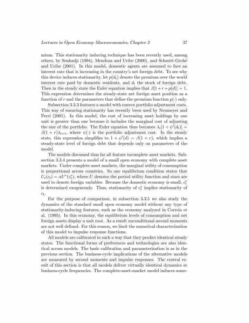
Lectures in Open Economy Macroeconomics, Chapter 3 37
mium. This stationarity inducing technique has been recently used, amongothers, by Senhadji (1994), Mendoza and Uribe (2000), and Schmitt-Groheand Uribe (2001). In this model, domestic agents are assumed to face aninterest rate that is increasing in the country’s net foreign debt. To see whythis device induces stationarity, let p(dt) denote the premium over the worldinterest rate paid by domestic residents, and dt the stock of foreign debt.Then in the steady state the Euler equation implies that β[1+r+p(d)] = 1.This expression determines the steady-state net foreign asset position as afunction of r and the parameters that define the premium function p(·) only.
Subsection 3.3.3 features a model with convex portfolio adjustment costs.This way of ensuring stationarity has recently been used by Neumeyer andPerri (2001). In this model, the cost of increasing asset holdings by oneunit is greater than one because it includes the marginal cost of adjustingthe size of the portfolio. The Euler equation thus becomes λt[1 + ψ′(dt)] =β(1 + r)λt+1, where ψ(·) is the portfolio adjustment cost. In the steadystate, this expression simplifies to 1 + ψ′(d) = β(1 + r), which implies asteady-state level of foreign debt that depends only on parameters of themodel.
The models discussed thus far all feature incomplete asset markets. Sub-section 3.3.4 presents a model of a small open economy with complete assetmarkets. Under complete asset markets, the marginal utility of consumptionis proportional across countries. So one equilibrium condition states thatUc(ct) = αU∗(c∗t ), where U denotes the period utility function and stars areused to denote foreign variables. Because the domestic economy is small, c∗tis determined exogenously. Thus, stationarity of c∗t implies stationarity ofct.
For the purpose of comparison, in subsection 3.3.5 we also study thedynamics of the standard small open economy model without any type ofstationarity-inducing features, such as the economy analyzed in Correia etal. (1995). In this economy, the equilibrium levels of consumption and netforeign assets display a unit root. As a result unconditional second momentsare not well defined. For this reason, we limit the numerical characterizationof this model to impulse response functions.
All models are calibrated in such a way that they predict identical steadystates. The functional forms of preferences and technologies are also iden-tical across models. The basic calibration and parameterization is as in theprevious section. The business-cycle implications of the alternative modelsare measured by second moments and impulse responses. The central re-sult of this section is that all models deliver virtually identical dynamics atbusiness-cycle frequencies. The complete-asset-market model induces some-

38 Martın Uribe
what smoother consumption dynamics but similar implications for hoursand investment.
3.3.1 Endogenous Discount Factor Without Internalization(Model 1a)
Consider an alternative formulation of the endogenous discount factor modelwhere domestic agents do not internalize the fact that their discount fac-tor depends on their own levels of consumption and effort. Alternatively,suppose that the discount factor depends not upon the agent’s own con-sumption and effort, but rather on the average per capita levels of thesevariables. Formally, preferences are described by (6.1), (3.2), and
θt+1 = β(ct, ht)θt t ≥ 0, (3.16)
where ct and ht denote average per capital consumption and hours, whichthe individual household takes as given.
The first-order conditions of the household’s maximization problem are(3.2), (3.4)-(3.7), (3.16) holding with equality and:
λt = β(ct, ht)(1 + rt)Etλt+1 (3.17)
λt = Uc(ct, ht) (3.18)
−Uh(ct, ht) = λtAtFh(kt, ht) (3.19)
λt[1+Φ′(kt+1−kt)] = β(ct, ht)Etλt+1
[At+1Fk(kt+1, ht+1) + 1 − δ + Φ′(kt+2 − kt+1)
]
(3.20)In equilibrium, individual and average per capita levels of consumption andeffort are identical. That is,
ct = ct (3.21)
andht = ht. (3.22)
A competitive equilibrium is a set of processes {dt, ct, ht, ct, ht, yt, it,kt+1, λt, rt, At} satisfying (3.4)-(3.7), (3.13), (3.14), (3.17)-(3.22) all hold-ing with equality, given A0, d−1, and k0 and the stochastic process {εt}.Note that the equilibrium conditions include one Euler equation less, equa-tion (3.10), and one variable less, ηt, than the standard endogenous-discount-factor model of subsection 3.1. This feature facilitates the computation ofthe equilibrium dynamics using perturbation methods.3
We evaluate the model using the same functional forms and parametervalues as in Model 1.
3It is remarkable that the degree of computational complexity is reversed when the

Lectures in Open Economy Macroeconomics, Chapter 3 39
3.3.2 Debt Elastic Interest Rate (Model 2)
In Model 2, stationarity is induced by assuming that the interest rate facedby domestic agents, rt, is increasing in the aggregate level of foreign debt,which we denote by dt. Specifically, rt is given by
rt = r + p(dt), (3.23)
where r denotes the world interest rate and p(·) is a country-specific interestrate premium. The function p(·) is assumed to be strictly increasing.
Preferences are given by equation (6.1). Unlike in the previous model,preferences are assumed to display a constant subjective rate of discount.Formally,
θt = βt,
where β ∈ (0, 1) is a constant parameter.The representative agent’s first-order conditions are (3.4)-(3.7) holding
with equality andλt = β(1 + rt)Etλt+1 (3.24)
Uc(ct, ht) = λt, (3.25)
−Uh(ct, ht) = λtAtFh(kt, ht). (3.26)
λt[1+Φ′(kt+1−kt)] = βEtλt+1
[At+1Fk(kt+1, ht+1) + 1 − δ + Φ′(kt+2 − kt+1)
].
(3.27)Because agents are assumed to be identical, in equilibrium aggregate percapita debt equals individual debt, that is,
dt = dt. (3.28)
A competitive equilibrium is a set of processes {dt, dt+1, ct, ht, yt, it, kt+1, rt, λt}∞t=0
satisfying (3.4)-(3.7), and (3.23)-(3.28) all holding with equality, given (3.14),A0, d−1, and k0.
We adopt the same forms for the functions U , F , and Φ as in Model 1.We use the following functional form for the risk premium:
p(d) = ψ2
(ed−d − 1
),
computational technique consists in iterating a Bellman equation over a discretized statespace. The economy with a noninternalized discount factor features an externality, whichwhich complicates significantly the task of computing the equilibrium by value functioniterations. A similar comment applies to the computation of equilibrium in a modelwith an interest-rate premium that depends on the aggreage level of external debt to bediscussed in the next subsection.

40 Martın Uribe
where ψ2 and d are constant parameters.We calibrate the parameters γ, ω, α, φ, r, δ, ρ, and σε using the values
shown in table 3.1. We set the subjective discount factor equal to the worldinterest rate; that is,
β =1
1 + r.
The parameter d equals the steady-state level of foreign debt. To see this,note that in steady state, the equilibrium conditions (3.23) and (3.24) to-gether with the assumed form of the interest-rate premium imply that1 = β
[1 + r + ψ2
(ed−d − 1
)]. The fact that β(1 + r) = 1 then implies
that d = d. If follows that in the steady state the interest rate premium isnil. We set d so that the steady-state level of foreign debt equals the oneimplied by Model 1. Finally, we set the parameter ψ2 so as to ensure thatthis model and Model 1 generate the same volatility in the current-account-to-GDP ratio. The resulting values of β, d, and ψ2 are given in table 2.
Table 3.3: Model 2: Calibration of Parameters Not Shared With Model 1
β d ψ2
0.96 0.7442 0.000742
3.3.3 Portfolio Adjustment Costs (Model 3)
In this model, stationarity is induced by assuming that agents face convexcosts of holding assets in quantities different from some long-run level. Pref-erences and technology are as in Model 2. In contrast to what is assumedin Model 2, here the interest rate at which domestic households can borrowfrom the rest of the world is constant and equal to the world interest, thatis, equation (3.13) holds. The sequential budget constraint of the householdis given by
dt = (1 + rt−1)dt−1 − yt + ct + it + Φ(kt+1 − kt) +ψ3
2(dt − d)2, (3.29)
where ψ3 and d are constant parameters defining the portfolio adjustmentcost function. The first-order conditions associated with the household’smaximization problem are (3.5)-(3.7), (3.25)-(3.27), (3.29) holding withequality and
λt[1 − ψ3(dt − d)] = β(1 + rt)Etλt+1 (3.30)

Lectures in Open Economy Macroeconomics, Chapter 3 41
This optimality condition states that if the household chooses to borrow anadditional unit, then current consumption increases by one unit minus themarginal portfolio adjustment cost ψ3(dt − d). The value of this increase inconsumption in terms of utility is given by the left-hand side of the aboveequation. Next period, the household must repay the additional unit of debtplus interest. The value of this repayment in terms of today’s utility is givenby the right-hand side. At the optimum, the marginal benefit of a unit debtincrease must equal its marginal cost.
A competitive equilibrium is a set of processes {dt, ct, ht, yt, it, kt+1, rt, λt}∞t=0
satisfying (3.5)-(3.7), (3.13), (3.25)-(3.27), (3.29), and (3.30) all holding withequality, given (3.14), A0, d−1, and k0.
Preferences and technology are parameterized as in Model 2. The para-meters γ, ω, α, φ, r, δ, ρ, and σε take the values displayed in table 3.1. Asin model 2, the subjective discount factor is assumed to satisfy β(1+r) = 1.This assumption and equation (3.30) imply that the parameter d determinesthe steady-state level of foreign debt (d = d). We calibrate d so that thesteady-state level of foreign debt equals the one implied by models 1, 1a,and 2 (see table 3.3). Finally, we assign the value 0.00074 to ψ3, whichensures that this model and model 1 generate the same volatility in thecurrent-account-to-GDP ratio. This parameter value is almost identical tothat assigned to ψ2 in model 2. This is because the log-linearized versionsof models 2 and 3 are almost identical. Indeed, the models share all equilib-rium conditions but the resource constraint (equations (3.4) and (3.29)), theEuler equations associated with the optimal choice of foreign bonds (equa-tions (3.24) and (3.30)), and the interest rate faced by domestic households(equations (3.13) and (3.23)). The log-linearized versions of the resourceconstraints are the same in both models. The log-linear approximation tothe domestic interest rate is given by 1 + rt = ψ2d(1 + r)−1dt in Model 2and by 1 + rt = 0 in Model 3. In turn, the log-linearized versions of theEuler equation for debt are λt = ψ2d(1 + r)−1dt + Etλt+1 in model 2 andλt = ψ3ddt + Etλt+1 in Model 3. It follows that for small values of ψ2 andψ3 satisfying ψ2 = (1 + r)ψ3 models 2 and 3 will imply similar dynamics.
3.3.4 Complete Asset Markets (Model4)
All model economies considered thus far feature incomplete asset markets.In those models agents have access to a single financial asset that pays arisk-free real rate of return. In the model studied in this subsection, agentshave access to a complete array of state-contingent claims. This assumptionper se induces stationarity in the equilibrium dynamics.

42 Martın Uribe
Preferences and technology are as in model 2. The period-by-periodbudget constraint of the household is given by
Etrt+1bt+1 = bt + yt − ct − it − Φ(kt+1 − kt), (3.31)
where rt+1 is a stochastic discount factor such that the period-t price ofa random payment bt+1 in period t + 1 is given by Etrt+1bt+1. Note thatbecause Etrt+1 is the price in period t of an asset that pays 1 unit of goodin every state of period t+1, it follows that 1/[Etrt+1] denotes the risk-freereal interest rate in period t. Households are assumed to be subject to ano-Ponzi-game constraint of the form
limj→∞
Etqt+jbt+j ≥ 0, (3.32)
at all dates and under all contingencies. The variable qt represents thestochatic discount factor between periods 0 and t, such that the period-0price of a random payment bt in period t is given by E0qtbt. We have thatqt satisfies
qt = r1r2 . . . rt,
with q0 ≡ 1. The first-order conditions associated with the household’s max-imization problem are (3.5), (3.6), (3.25)-(3.27), (3.31), and (3.32) holdingwith equality and
λtrt+1 = βλt+1. (3.33)
A difference between this expression and the Euler equations that arise inthe models with incomplete asset markets studied in previous sections is thatunder complete markets in each period t there is one first-order conditionfor each possible state in period t + 1, whereas under incomplete marketsthe above Euler equation holds only in expectations.
In the rest of the world, agents have access to the same array of financialassets as in the domestic economy. Consequently, one first-order conditionof the foreign household is an equation similar to (3.33). Letting starredletters denote foreign variables or functions, we have
λ∗t rt+1 = βλ∗t+1. (3.34)
Note that we are assuming that domestic and foreign households share thesame subjective discount factor. Combining the domestic and foreign Eulerequations—equations (3.33) and (3.34)—yields
λt+1
λt=λ∗t+1
λ∗t.

Lectures in Open Economy Macroeconomics, Chapter 3 43
This expression holds at all dates and under all contingencies. This meansthat the domestic marginal utility of consumption is proportional to itsforeign counterpart. Formally,
λt = ξλ∗t ,
where ξ is a constant parameter determining differences in wealth acrosscountries. We assume that the domestic economy is small. This means thatλ∗t must be taken as an exogenous variable. Because we are interested onlyin the effects of domestic productivity shocks, we assume that λ∗t is constantand equal to λ∗, where λ∗ is a parameter. The above equilibrium conditionthen becomes
λt = ψ4, (3.35)
where ψ4 ≡ ξλ∗ is a constant parameter.A competitive equilibrium is a set of processes {ct, ht, yt, it, kt+1, λt}∞t=0
satisfying (3.5), (3.6), (3.25)-(3.27), and (3.35), given (3.14), A0, and k0.The functions U , F , and Φ are parameterized as in the previous models.
The parameters γ, β, ω, α, φ, δ, ρ, and σε take the values displayed intables 3.1 and 3.3. The parameter ψ4 is set so as to ensure that the steady-state level of consumption is the same in this model as in models 1 to 3.
3.3.5 The Nonstationary Case (Model 5)
For comparison with the models considered thus far, in this section we de-scribe a version of the small open economy model that displays no station-arity. In this model (a) The discount factor is constant; (b) the interestrate at which domestic agents borrow from the rest of the world is constant(and equal to the subjective discount factor); (c) agents face no frictionsin adjusting the size of their portfolios; and (d) markets are incomplete inthe sense that domestic households have only access to a single risk-freeinternational bond. This specification of the model induces a random walkcomponent in the equilibrium marginal utility of consumption and the netforeign asset position.
A competitive equilibrium in the nonstationary model is a set of processes{dt, ct, ht, yt, it, kt+1, rt, λt}∞t=0 satisfying (3.4)-(3.7), (3.13), and (3.24)-(3.27) all holding with equality, given (3.14), A0, d−1, and k0. We calibratethe model using the parameter values displayed in tables 3.1 and 3.3.

44 Martın Uribe
3.3.6 Quantitative Results
Table 3.4 displays a number of unconditional second moments of interestobserved in the data and implied by models 1 - 4.4 For all models, wecompute the equilibrium dynamics by solving a log-linear approximation tothe set of equilibrium conditions. The appendix shows the log-linear versionof model 1. The Matlab computer code used to compute the unconditionalsecond moments and impulse response functions for all models presented inthis section is available at www.econ.duke.edu/∼uribe.
Although the focus of this section is not to assess the models’ abilities tomatch the data, as a reference we include in the first column of the table theobserved second moments using Canadian data. As pointed out by Men-doza (1991), the small open real business cycle model captures a number offeatures of business cycles in Canada. Specifically, as in the data, all fourmodels predict the following ranking of volatilities, in ascending order, con-sumption, output, and investment. The models also correctly predict thatthe components of aggregate demand and hours are procyclical, and thatthe correlation of the trade balance with GDP is close to zero.5 The modelsoverestimate the procyclicality of labor. In the data the correlation betweenhours and output is 0.8, whereas the models imply a perfect correlation. Aspointed out earlier, this implication of the models is driven by the assumedpreference specification.
The main result of this section is that regardless of how stationarity isinduced, the model’s predictions regarding second moments are virtuallyidentical. This result is evident from table 3.4. The only noticeable differ-ence arises in model 4, the complete markets case, which as expected predictsless volatile consumption. The low volatility of consumption in the completemarkets model introduces an additional difference between the predictionsof this model and models 1-3. Because consumption is smoother in model4, its role in determining the cyclicality of the trade balance is smaller. As aresult, model 4 predicts that the correlation between output and the tradebalance is positive, whereas models 1-3 imply that it is negative.
Figure 3.3 demonstrates that models 1-5 also imply virtually identicalimpulse response functions to a technology shock. Each panel shows theimpulse response of a particular variable in the six models. For all variables
4Model 5 is nonstationary, and therefore does not have well defined unconditionalsecond moments.
5Indeed, models 1-3 predict correctly that the trade balance is countercyclical. Thecorrelation is so close to zero, however, that its sign does depend on the solution methodemployed. Mendoza, for example, approximates the solution to model 1 by discretizingthe state space and finds a small but positive correlation.

Lectures in Open Economy Macroeconomics, Chapter 3 45
but consumption and the trade-balance-to-GDP ratio, the impulse responsefunctions are so similar that to the naked eye the graph appears to showjust a single line. Again, the only small but noticeable difference is givenby the responses of consumption and the trade-balance-to-GDP ratio inthe complete markets model. In response to a positive technology shock,consumption increases less when markets are complete than when marketsare incomplete. This in turn, leads to a smaller decline in the trade balancein the period in which the technology shock occurs.

46 Martın Uribe
3.4 Appendix
3.4.1 Log-Linearization of the Equilibrium Conditions
Let xt ≡ log(xt/x) denote the log-deviation of xt from its steady-state value.Then, taking a first-order log-linearization of the model we get:
stbdt = stbr
1 + rrt−1 + stb(1 + r)dt−1 − r[yt − scct − siit]
yt = At + αkt + (1 − α)ht
kt+1 = (1 − δ)kt + δit
λt =r
1 + rrt + εβcct + εβhht +Etλt+1
λt =(1 − β)εc
(1 − β)εc − βεβc[εccct + εchht] −
βεβc(1 − β)εc − βεβc
[ηt + εβccct + εβchht]
ηt = (1 − β)[εcEtct+1 + εhEtht+1] + β[Etηt+1 + εβcct + εβhht]
(1 − β)εh(1 − β)εh + βεβh
[εhcct+εhhht]+βεβh
(1 − β)εh + βεβh[ηt+εβhcct+εβhhht] = λt+At+αkt−αht
λt + φkkt+1 − φkkt = εβcct + εβhht +Etλt+1 + β(β−1 + δ − 1)[EtAt+1
+(1 − α)Etht+1 − (1 − α)kt+1 + βφkEtkt+2 − βφkkt+1
rt = 0
At = ρAt−1 + εt,
where εβc ≡ cβc/β, εβh ≡ hβh/β, εβcc ≡ cβcc/βc, εβch ≡ hβch/βc, εc ≡cUc/U , εcc = cUcc/Uc, εch = hUch/Uc, stb ≡ tb/y, sc ≡ c/y, si = i/y.In the log-linearization we are using the particular forms assumed for theproduction function and the capital adjustment cost function.
3.5 Exercise
Real Business Cycles in a Small Open Economy with an in-ternalized debt-elastic interest-rate premium
Consider a variation of the small open economy RBC model with a debt elas-tic interest rate premium studied in Schmitt-Grohe and Uribe (SGU) (JIE,2003, section 3, model 2) that allows agents to internalize the dependence of

Lectures in Open Economy Macroeconomics, Chapter 3 47
the interest rate premium on the level of debt. . Specifically, suppose thatthe function p(·) depends on the individual debt position, dt, rather than onthe aggregate per capita level of debt, dt.
1. Derive the model’s equilibrium conditions.
2. Use the same forms for the functions U , F , Φ, and p as in SGU.Calibrate the parameters γ, ω, α, φ, r, δ, ρ, σε, β, d, and ψ2 usingtables 1 and 2 in SGU. Calculate the model’s nonstochastic steadystate and compare it to that of model 2 in SGU.
3. Compute the unconditonal standard deviation, serial correlation, andcorrelation with output of output, consumption, investment, hours, thetrade balance-to-output ratio, and the current account-to-output ratioimplied by the model. Compare these statistics to those associatedwith model 2 in SGU (reported in their table 3).
4. Compute the impulse response functions of output, consumption, in-vestment, hours, the trade balance-to-output ratio, and the currentaccount-to-output ratio implied by the model. Compare these im-pulse responses to those associated with model 2 in SGU (shown intheir figure 1).

48 Martın Uribe
Table 3.4: Observed and Implied Second Moments
Data Model 1 Model 1a Model 2 Model 3 Model 4
Volatilities:std(yt) 2.8 3.1 3.1 3.1 3.1 3.1std(ct) 2.5 2.3 2.3 2.7 2.7 1.9std(it) 9.8 9.1 9.1 9 9 9.1std(ht) 2 2.1 2.1 2.1 2.1 2.1std( tbtyt
) 1.9 1.5 1.5 1.8 1.8 1.6
std( catyt
) 1.5 1.5 1.5 1.5
Serial Correlations:corr(yt, yt−1) 0.61 0.61 0.61 0.62 0.62 0.61corr(ct, ct−1) 0.7 0.7 0.7 0.78 0.78 0.61corr(it, it−1) 0.31 0.07 0.07 0.069 0.069 0.07corr(ht, ht−1) 0.54 0.61 0.61 0.62 0.62 0.61corr( tbtyt
, tbt−1
yt−1) 0.66 0.33 0.32 0.51 0.5 0.39
corr( catyt, cat−1
yt−1) 0.3 0.3 0.32 0.32
Correlations with Output:corr(ct, yt) 0.59 0.94 0.94 0.84 0.85 1corr(it, yt) 0.64 0.66 0.66 0.67 0.67 0.66corr(ht, yt) 0.8 1 1 1 1 1corr( tbtyt
, yt) -0.13 -0.012 -0.013 -0.044 -0.043 0.13
corr( catyt, yt) 0.026 0.025 0.05 0.051
Note. The first column was taken from Mendoza (1991). Stan-dard deviations are measured in percent per year.

Lectures in Open Economy Macroeconomics, Chapter 3 49
Figure 3.3: Impulse Response to a Unit Technology Shock in Models 1 - 5
0 2 4 6 8 100
0.5
1
1.5
2Output
0 2 4 6 8 100
0.5
1
1.5Consumption
0 2 4 6 8 10−5
0
5
10Investment
0 2 4 6 8 100
0.5
1
1.5Hours
0 2 4 6 8 10−1
−0.5
0
0.5
1Trade Balance / GDP
0 2 4 6 8 10−1
−0.5
0
0.5
1Current Account / GDP
Note. Solid line: Endogenous discount factor model; Squares:Endogenous discount factor model without internalization;Dashed line: Debt-elastic interest rate model; Dash-dotted line:Portfolio adjustment cost model; Dotted line: complete assetmarkets model; Circles: Model without stationarity inducing el-ements.

50 Martın Uribe

Chapter 4
Solving Dynamic GeneralEquilibrium Models ByLinear Approximation
The equilibrium conditions of the simple real business cycle model we stud-ied in the previous chapter takes the form of a nonlinear stochastic vectordifference equation. Reduced forms of this sort are common in Macroeco-nomics. A problem that one must face is that, in general, it is impossibleto solve such systems. But fortunately one can obtain good approximationsto the true solution in relatively easy ways. In the previous chapter, weintroduced one particular strategy, consisting in linearizing the equilbriumconditions around the nonstochastic steady state. Here we explain in detailhow to solve the resulting system of linear stochastic difference equations.In addition, we show how to use the solution to compute second momentsand impuse response functions.
Consider a vector xt of order n× 1 whose law of motion is of the form
AEtxt+1 = Bxt +C (4.1)
It is convenient to partition xt into two components
xt ≡[stct
].
The vector st is of order ns×1 and contains either endogenous predeterminedvariables that cannot adjust contemporaneously to news, or exogenous vari-ables. The vector ct is of order nc × 1 and contains endogenous variables
51

52 Martın Uribe
that can adjust contemporaneously to news. The vectors st and ct are alsoreferred to as the state and the control of the system, respectively. Us-ing the RBC model of the previous chapter as an example, we have thatthe capital stock and the net debt position of the economy are endogenousstate variables, the productivity shock is an exogenous state variable, andconsumption and hours are two of the control variables of the system. Ofcourse, we have that ns+nc = n. We further partitiion the state vector intothe endogenous component, sent , and the exogenous component, sext ,
st ≡[sentsext
],
where sent is of order nen×1 and sext is of order nex×1, with nen+nex = ns.The initial conditions of the system is
s0 = s,
where s is an ns × 1 vector of constants. There are no initial conditions forthe control variables. Instead, we impose terminal conditions, by requiringthat at each point the variables of the system be expected not to explode.Formally,
limj→∞
|Etxt+j | <∞
The source of uncertainty in the system is a vector µt of innovations to thestate of the economy. That is,
µt+1 ≡ st+1 −Etst+1,
The vector µt is given by
µt =[
∅εt
],
where εt is of order nex × 1 and denotes the innovation to the exogenousstate vector and is i.i.d. with mean ∅ and variance/covariance matrix Σε.
The n×n matrix A may be singular, reflecting the presence of equationsinvolving only elements of xt (i.e., involving no elements of Etxt+1). Oneshould not interpret the singularity of A as indicating multiple solutions orno solution to the system.To see this, consider the following example:
xt+1 = axt + yt
yt = bxt

Lectures in Open Economy Macroeconomics, Chapter 4 53
with xt a predetermined state variable and yt a non-predetermined controlvariable and |a+ b| < 1. If one writes the system in the form given by (4.1)
A =[
1 00 0
]and B =
[a 1b −1
]
Clearly, A is not invertible. However, the system has a unique solution givenby
xt = (a+ b)tx0; t ≥ 0.
We look for the recursive representation of the solution to the system (4.1),which is of the form:
ct = Πst + L
Etst+1 = Φst +N
The nonstochastic steady state (4.1) is given by a couple of vectors c ands satisfying [
sc
]≡ x = (A−B)−1C
Define xt = xt − x as the deviation of xt from its steady-state value. Thenwe can concentrate in solving the following homogeneous system in xt:
AEtxt+1 = Bxt
Next, we show how to compute the matrices Φ, Π, L, and N .
4.1 The Schur Decomposition Method
To solve the above system, we use the generalized Schur decomposition ofthe matrices A and B.1 The generalized Schur decomposition of A and B isgiven by upper triangular matrices a and b and orthonormal matrices q andz satisfying:2
qAz = a
andqBz = b.
Letyt ≡ z′xt.
1More formal descriptions of the method can be found in Klein (2000) and Sims (1996).2Recall that a matrix a is said to be upper triangular if elements aij = 0 for i > j. A
matrix z is orthonormal if z′z = zz′ = I.

54 Martın Uribe
Then we have thataEtyt+1 = byt
Now partition a, b, z, and yt as
a =[a11 a12
0 a22
], b =
[b11 b120 b22
]; z =
[z11 z12z21 z22
]; yt =
[y1t
y2t
],
where a22 and b22 are of order nc × nc, z12 is of order ns × nc, and y2t is of
order nc × 1. Then we have that
a22Ety2t+1 = b22y
2t ,
orb−122 a22Ety
2t+1 = y2
t .
Assume, without loss of generality, that the ratios abs(aii/bii) are decreasingin i. Suppose further that the number of ratios less than unity is exactlyequal to the number of control variables, nc, and that the number of ratiosgreater than one is equal to the number of state variables, ns. By construc-tion, the eigenvalues of b−1
22 a22 are all less than unity in modulus.3 Thus,the requirement limj→∞ |Ety2
t+j | <∞ is satisfied only if y2t = 0. In turn, by
the definition of y2t , this restriction implies that
z′12st + z′22ct = 0,
orct = −z′22
−1z′12st;
so thatΠ = −z′22
−1z′12.
The fact that y2t = 0 also implies that
a11y1t+1 = b11y
1t ,
ory1t+1 = a11
−1b11y1t
Nowy1t = z′11st + z′21ct
3Here we are applying a number of properties of upper triangular matrices. Namely,(a) The inverse of a nonsingular upper triangular matrix is upper triangular. (b) theproduct of two upper triangular matrices is upper triangular. (c) The eigenvalues of anupper triangular matrix are the elements of its main diagonal.

Lectures in Open Economy Macroeconomics, Chapter 4 55
soy1t = [z′11 − z′21z
′22
−1z′12]st.
Combining this expression with the equation describing the evolution of ytshown two lines above, we get
st+1 = [z′11 − z′21z′22
−1z′12]
−1a11−1b11[z′11 − z′21z
′22
−1z′12]st;
so that
Φ = [z′11 − z′21z′22
−1z′12]
−1a11−1b11[z′11 − z′21z
′22
−1z′12].
We can simplify this expression for Π by using the following restrictions:
I = z′z =[z′11z11 + z′21z21 z′11z12 + z′21z22z′12z11 + z′22z21 z′12z12 + z′22z22
]
to write:4
Π = z21z−111
Φ = z11a−111 b11z
−111 .
Finally, by the definitions of ct and st, it follows that
L = c− Πs
andN = s− Φs
4.1.1 Matlab Code
Paul Klein of the University of Western Ontario has written Matlab pro-grams that compute the matrices Φ and Π given A, B, and ns. The setof programs consists of three files, solab.m, qzswitch.m, and qzdiv.m and isavailable on Klein’s website, http://www.ssc.uwo.ca/economics/faculty/klein/.The programs qzswitch.m and qzdiv.m were created by Chris Sims of Prince-ton University.
4To obtain K use the element (2, 1) of z′z. To obtain the reduced expression forΦ, use element (2, 1) of z′z to get z′
12z11 = −z′22z21. Pre multiply by z′
22−1
and postmultiply by z−1
11 to get z′22
−1z′12 = −z21z11
−1. Use this expression to eliminate z′22
−1z′12
From the square bracket in the expression for Φ. Then this square bracket becomes [z′11 +
z′21z21z11
−1]. Now use element (1, 1) of z′z to write z′21z21 = I−z′
11z11. Using this equationto eliminate z′
21z21 from the expression in square brackets, we get [z′11 +(I−z′
11z11)z11−1],
which is simply z−111 .

56 Martın Uribe
4.2 Computing Second Moments
Start with the equilibrium law of motion of the deviation of the state vectorwith respect to its steady-state value, which is given by
st+1 = Φst + µt+1, (4.2)
LetΣs ≡ Ests
′t
denote the unconditional variance/covariance matrix of st and
Σµ ≡[∅ ∅∅ Σε
]
the variance/covariance matrix of µt. Then we have that
Σs = ΦΣsΦ′ + Σµ.
We will describe three numerical methods to compute Σs.
4.2.1 Method 1
Suppose Φ can be decomposed as Φ = RΓR−1, where Γ is a diagonal matrix.Then letting
st = R−1st,
we can writest+1 = Γst +R−1µt+1.
Now defining Σs = Estst and Σµ = R−1ΣµR−1′, we have
Σs = ΓΣsΓ′ + Σµ
It follows that
Σs,ij =Σµ,ij
1 − ΓiΓji, j = 1, . . . ns,
where Σs,ij denotes the element of Σs located in the ith row and the jthcolumn (a similar notation applies for Σµ,ij) and Γi denotes the ith diagonalelement of Γ. Now use the fact that st = Rst to obtain
Σs = RΣsR′.

Lectures in Open Economy Macroeconomics, Chapter 4 57
4.2.2 Method 2
Apply the following iterative method:
Σs,t+1 = ΦΣs,tΦ′ + Σµ
Σs,0 = I
Stop when Σs,t does not change much as t increases.
4.2.3 Method 3
The following procedure, called doubling algorithm, is a faster version of theone described above.
Σs,t+1 = ΦtΣs,tΦ′t + Σµ,t
Φt+1 = ΦtΦt
Σµ,t+1 = ΦtΣµ,tΦ′t + Σµ,t
Σs,0 = I
Φ0 = Φ
Σµ,0 = Σµ
4.2.4 Other second moments
Once the variance/covariance matrix of the state vector has been computed,it is easy to find other second moments of interest. Consider for instancethe variance/covariance matrix Ests′t−j for j > 0.
Ests′t−j = E[Φj st−j +
j−1∑
h=0
Φhµt−h]s′t−jl
= ΦjEst−1s′t−j
= ΦjΣs
Similarly, consider the variance covariance matrix of linear combinations ofthe state vector st. For instance, the co-state, or control vector ct is givenby ct = Πst. Then
Ectc′t = Π[Ests′t]Π
′
= ΠΣsΠ′.

58 Martın Uribe
and, more generally,
Ect c′t−j = Π[Ests′t−j]Π
′
= ΠΦjΣsΠ′,
for j ≥ 0.
4.3 Impulse Response Functions
The impulse response function traces the expected behavior of the systemfrom period 0 on given information available in period 0, in a situation wherein period 0 all but one (or some) element(s) of the state vector take theirsteady-state values. Let the initial state of the system be s, that is, s0 = s.Using the law of motion Etst+1 = Φst for the state vector and the law ofiterated expectations we get that the impulse response of the state vectorin period t is given by
IR(st) ≡ E0st = Πts; t ≥ 0.
The response of the vector of controls ct is given by
IR(ct) = ΠΦts.
4.4 Higher Order Approximations
In this chapter, we focused on a first-order approximation to the solu-tion of a nonlinear system of stochastic difference equations of the formEtf(xt+1, xt) = 0.. But higher order approximations are relatively easy toobtain. Indeed, there is a sense in which higher order approximations aresimpler than the first order approximation. Namely, obtaining a higher-order approximation to the solution of the non-linear system is a sequentialprocedure. Specifically, the coefficients of the ith term of the jth-order ap-proximation are given by the coefficients of the ith term of the ith orderapproximation, for j > 1 and i < j. So if the first-order approximationto the solution is available, then obtaining the second order approximationrequires only to compute the coefficients of the quadratic terms, since thecoefficients of the linear terms are those of the first order approximation.More importantly, obtaining the coefficients of the ith order terms of theapproximate solution given all lower-order coefficients involves solving a lin-ear system of equations.

Lectures in Open Economy Macroeconomics, Chapter 4 59
Schmitt-Grohe and Uribe (2004) describe in detail how to obtain a seond-order approximation to the solution of the nonlinear system and provideMATLAB code that implements the approximation.

60 Martın Uribe

Chapter 5
Business Cycles In EmergingEconomies (In Progress)
In discussions of business cycles in small open economies, a critical distinc-tion is between developed and emerting economies. The group of emergingeconomies is composed by middle income countries with relatively smalllevels of market capitalization tradable internationally,
5.1 Some Empirical Regularities
A striking difference between developed and emerging economies is that ob-served business cycles in emerging countries are twice as volatile than indeveloped countries. Table 5.1 illustrates this contrast by displaying keybusiness-cycle properties in Argentina and and Canada. The volatility ofdetrended output is 4.6 in Argentina but only 2.8 in Canada. Another re-markable difference between developing and developed countries suggestedby the table is that the trade balance-to-output ratio is much more counter-cylical in emerging countries than in develped countries. Periods of economicboom (contraction) are characterized by relatively larger trade deficits (sur-pluses) in emerging countries than in develped countries. A third differencebetween developed and devellping economies that one may extrapolate fromthe table is that in the latter group consumption appears to be more volatilethan output at business-cycle frequences, whereas the reverse is the case inthe former set of countries. Two additional differences between the businesscycle in Argentina and Canada are that in Argentina, the correlation of thecomponents of aggregate demand with GDP are twice as high as in Canada,and that in Argentina hours and productivity are less correlated with GDP
61

62 Martın Uribe
Table 5.1: Business Cycles in Argentina and Canada
Variable σx corr(xt, xt−1) corr(xt, GDPt)GDPArgentina 4.6 0.79 1Canada 2.8 0.61 1ConsumptionArgentina 5.4 0.96Canada 2.5 0.70 0.59InvestmentArgentina 13.3 0.94Canada 9.8 0.31 0.64TB/GDPArgentina 2.3 -0.84Canada 1.9 0.66 -0.13HoursArgentina 4.1 0.76Canada 2.0 0.54 0.80ProductivityArgentina 3.0 0.48Canada 1.7 0.37 0.70
Source: Mendoza (1991), Kydland and Zarazaga (1997). For Ar-gentina, data on hours and productivity are limited to the manufac-turing sector.
than in Canada.One dimension along which business cycles in Argentina and Canada
are similar is the procyclicality of consumption, investment, hours,and pro-ductivity. In both types of country, these variables move in tandem withouput.
The differences between the business cycles of Argentina and Canadaturn out to hold much more generally. In effect, table 5.2, taken fromAguiar and Gopinath (2004) displays average business cycle facts in de-veloped and emerging economies. The table averages second moments ofdetrended data for a group of 13 emerging countries and a group of 13 smalldeveloped countries (the list of countries appears at the foot of the table).

Lectures in Open Economy Macroeconomics, Chapter 5 63
Table 5.2: Business Cycles: Emerging Vs. Developed Economies
Emerging DevelopedMoment Countries Countriesσy 2.02 1.04σ∆y 1.87 0.95ρy 0.86 0.9ρ∆y 0.23 0.09σc/σy 1.32 0.94σi/σy 3.96 3.42σtb/y 2.09 0.71ρtb/y,y -0.58 -0.26ρc,y 0.74 0.69ρi,y 0.87 0.75
Note: Average values of moments for 13 emerging countries and 13developed countries. Emerging countries: Argentina, Brazil, Ecuador,Israel, Korea, Malaysia, Mexico, Peru, Philippines, Slovak Republic,South Africa, Thailand, and Turkey. Developed Countires: Australia,Austria, Belgium, Canada, Denmark, Finland, Netherlands, New Ze-land, Norway, Portugal, Spain, Sweden, Switzerland. Data are de-trended using a band-pass filter including frequencies between 6 and32 quarters with 12 leads and lags.Source: Aguiar and Gopinath (2004).
For all countries, the time series are at least 40 quarters long. The datais detrended using a band-pass filter that leaves out all frequencies above32 quarters and below 6 quarters. The table concurs with the conclusionsdrawn from the comparison of cusiness cycles in Argentina and Canada. Inparticular, emerging countires are significantly more volatile and display amuch more countercyclical trade-balance share, than developed countries.Also, consumption is more volatile than output in emerging countries butless volatile than output in developed countries.
5.2 Trends and Cycles
Aguiar and Gopinath (2004) argue that key differences between the businesscycle in developed and emerging countries can be explained by the fact that

64 Martın Uribe
in emerging countries permanent productivity shocks are relatively moreimportant than transitory productivity shocks vis-a-vis developed countries.
It is easy to imagine how this hypothesis can explain the higher volatilityof output in emerging countries. But how can difference in the relative im-portance of permanent and transitory shocks explain the observed strongercountercyclicality of the trade balance in emerging countries? Suppose firstthat the small open economy is hit by a positive transitory shock to pro-ductivity. Because the improvement in productivity is expected to revertto its mean, agents expect output to be higher in the short run than inthe long run. As a rexult, in this case the general tendency is to save partof the increase in output for consumption in the future. This tendency tosave dampens the response of consumption creating a tendency for the tradebalance to be procyclical. Consider now the case of a permanent shock thattakes the form of a mean reverting increase in the growth rate of produc-tivity.In this case, agents expect the level of output and productivity to behigher in the future than in the present. As a result, households have anincentive to borrow agains future income to expand present consumption,and firms have an incentive to invest in physical capital to take advantateof higher future higher productivity. In this situation, aggregate has a ten-dency to expand more vigorously than output, inducing a deterioration inthe trade balance. This explanation also provides intuition for why con-sumption should be expected to be more volatile the larger the importanceof permanent shocks relative to transitory disturbances.
5.2.1 A Small Open Economy With Nonstationary Shocks
Aguiar and Gopinath consider a version of the model with a debt-elasticinterest-rate premium presented in chapter 3 (section 3.3.2) augmented withnonstationary shocks a la King, Plosser, and Rebelo (1988b). Spedivically,suppose that the production technology takes the form
Yt = atKαt (Xtht)1−α, (5.1)
where Yt denotes ouput in period t, Kt denotes capital in period t, ht denoteshours worked in period t, and at and Xt represent productivity shocks.We use upper case letters to denote variables that will contain a trend inequilibrium, and lower case letters to denote varibles that do not contain atrend in equilibrium.
The productivity shock at is assumed to follow first-order autorregressiveprocess in logs. That is,
ln at+1 = ρa ln at + εat+1; .

Lectures in Open Economy Macroeconomics, Chapter 5 65
The productivity shock Xt is assumed to be nonstationary. Specifically, weassume that the growth rate of Xt,
gt ≡Xt
Xt−1,
follows a first-order autorregressive process of the form
ln(gt+1/g) = ρg ln(gt/g) + εat+1; .
The innovations εat and εgt are assumed to be mutually independent, i.i.d.,and to have mean zero and standard deviations σa and σg, respectively. Theparameter g is a measure of the average gross growth rate of the productivityfactor Xt.
Household face the following period-by-period budget constraint
Dt
1 + rt= Dt−1 − Yt + Ct + It +
φ
2Xt(Kt+1 − gKt)2. (5.2)
The nonstationary shock Xt appears in the adjustment const function to en-sure that adjustment costs grow at the same rate as the rest of the economyin the deterministic path. Similarly, to avoid a trend in hours worked, wemodify the specification of the interest-rate premium and the utility functionas follows:
rt = r + ψ2
(eDt/Xt−d − 1
),
and∞∑
t=0
βt[Ct − ω−1Xth
ωt
]1−γ − 11 − γ
. (5.3)
The variable Dt denotes the aggregate level of external debt per capita,which the household takes as exogenous. In equilibrium, we have that Dt =Dt.
Households are subject to a no-Ponzi-scheme constraint of the formlimj→∞Et
Dt+j∏js=0(1+rs)
≤ 0.
The household seeks to maximize the utility fucntion (5.3) subject to (5.1),(5.2) and the no-Ponzi-game constraint, taking as given the processes at, Xt,and rt and the initial conditions K0 and D−1.
5.2.2 Equilibrium
Define yt = Yt/Xt, ct = Ct/Xt, dt = Dt/Xt, and kt = Kt/Xt−1. Then, astationary competitive equilibrium is give by a stationary solution to thefollowing equations:

66 Martın Uribe
[ct − ω−1hωt ]−γ = λt
hω−1t = (1 − α)at
(ktgtht
)α
λt = β[1 + r + ψ2
(edt−d − 1
)]Etg
−γt+1λt+1
λt[1+φ(kt+1−g
gtkt)] = βEtg
−γt+1λt+1
[1 − δ + αat+1
(kt+1
gt+1ht+1
)α−1
+ φg
(kt+2 −
g
gt+1kt+1
)]
dt1 + rt
=dt−1
gt− at
(ktgt
)α
h1−αt + ct + it +
φ
2
(kt+1 −
g
gtkt
)2
rt = r + ψ2
(edt−d − 1
),
This zaga will be continued]

Chapter 6
Exchange-Rate-BasedInflation Stabilization
The main conclusion fromFor many emerging markets, business fluctuations are marked by balance-
of-payment crises. That is, sharp reallocations of domestic agents’ portfoliosagainst domestic assets and in favor of foreign assets. Often, the domesticasset household
1. Main elements of the model:
(a) Continuous-time model of a small, open, endowment economy
(b) Traded and nontraded goods
(c) Money is motivated by a cash-in-advance constraint
(d) The government sets the devaluation rare at a low level for Tperiods and then is expected to raise it to a higher permaenntlevel.
2. Results:
(a) Consumption increases on impact and remains constant at thishigher level until time T , when it falls to its long-run level (whichis lower than the pre-stabilizaiton level).
(b) The real exchange rate (the relative price of nontradables in termsof tradables) jumps up (appreciates) on impact, remains constantuntil period T , and then falls to its long-run level, (which is lowerthan its pre-stabilization level).
67

68 Martın Uribe
(c) The trade balance deteriorates on impact, remains constant un-til period T , and then jumps up to a level hgher than the oneprevailing before the announcement of the stabilization program.
(d) In period T , there is a BOP crisis, as agents reduce their moneyholdings in a discrete fashion in exchange for foreign bonds (thus,the central bank loses reserves in exactly the amount in which realbalances fall)
3. Intuition: In this model, the rate of devaluation acts as a tax on con-sumption. Thus, a temporary decline in the devaluation rate inducesintertemporal substitution in favor of current consumption and againstfuture consumption.

Lectures in Open Economy Macroeconomics, Chapter 6 69
Households
Households maximize∫ ∞
0e−ρt[u(cTt ) + v(cNt )] (6.1)
subject toWt = Etb
pt +Mt
Wt = rEtbpt + Etb
pt + P Tt [(yT − cTt ) + pt(yN − cNt )] − P Tt τt
Mt ≥ αP Tt (cTt + ptcNt )
where W denotes nominal financial wealth, M denotes nominal money bal-ances, b denotes holdings of a foreign-currency-denominated bond paying theconstant interest rate r in foreign currency, E denotes the nominal exchangerate, defined as the price of foreign currency in terms of domestic currency,cT and cN denote consumption of tradables and nontradables, respectively,yT and yN denote the endowments of tradables and nontradables, respec-tively, P Tt denotes the domestic curency price of tradbles, and p denotes thereal exchange rate, defined as the price of nontradables in terms of tradables.The foreign currency price of tradables is assumed to be equal to one and thelaw of one price is assumed to hold for tradables. Thus, P Tt = P ∗Et = Et.Finally, τt denote real lump-sum taxes measured in terms of tradables.
Let εt ≡ Et/Et denote the rate of devaluation. Use the first two con-straints to eliminate bpt ,
Wt
Et− EtEt
Wt
Et= r
Wt
Et− (r + Et/Et)
Mt
Et+ yT − cTt + pt(yN − cNt ) − τt
Let wt ≡ Wt/Et and mt = Mt/Et denote real financial wealth and realbalances measured in terms of tradables. Then the above expresion can bewritten as
wt = rwt − (r + εt)mt + yT − cTt + pt(yN − cNt ) − τt
In addition, households are subject to a no-Ponzi-game constraint of theform:
limt→∞
e−rtwt ≥ 0
The above two constraints are equivalent to the following intertemporalbudget constraint
w0 ≥∫ ∞
0e−rt
[(r + εt)mt − yT + cTt − pt(yN − cNt ) + τt
]dt

70 Martın Uribe
Under perfect foresight and free capital mobility, the domestic nominal in-terest rate, it, must satisfy the uncovered interst parity condition, that is,
it = r + εt
To the extent that the nominal interes rate is positive, the cash-in-advancewill hold with strict equality. Assuming that this is the case at all times(something that we will have to check when we characterize the equilib-rium), we can use the cash-in-advance constraint to eliminate mt from theintertemporal resource constraint
w0 ≥∫ ∞
0e−rt
[(1 + αit)(cTt + ptc
Nt ) + τt − yT − pty
N]
(6.2)
Households maximize (6.1) subject to (6.2). The first-order conditions are(6.2) holidng with equality and
u′(cTt ) = λ(1 + αit) (6.3)
v′(cNt )u′(cTt )
= pt (6.4)
w0 =∫ ∞
0e−rt
[(1 + αit)(cTt + ptc
Nt ) − yT − pty
N − τt]
(6.5)
The consolidated government
The government’s flow budget constraint is:
bgt = rbgt + τt +Mt
Et
Using the fact that mt = Mt/Et − εtmt we have
bgt − mt = rbgt + τt + εtmt
or, adding and subtracting rmt on the right-hand side
bgt − mt = r(bgt −mgt ) + τt + itmt
We will assume that the government is subject to a no-Ponzi-game constraintwhereby the limit of the present discounted value of the real value of its totalliabilities, mt − bgtmt, must be zero, that is
limt→∞
e−rt(mt − bgt ) = 0
The above two expressions imply that
m0 − bg0 =∫ ∞
0[itmt + τt]dt (6.6)

Lectures in Open Economy Macroeconomics, Chapter 6 71
Exchange rate policy
εt ={
εL t < TεH > εL t ≥ T
(6.7)
6.0.3 Market-clearing conditions
cNt = yN (6.8)
Combining equations (6.5) and (6.6) and taking into account that w0 =m0 + bp0 yields
b0 =∫ ∞
0e−rt
[cTt − yT
](6.9)
where b0 ≡ bp0 + bg0.

72 Martın Uribe

Chapter 7
Models of Balance ofPayments Crises
A balance of payments (BOP) crisis is a situation in which the private sectorchanges the composition of its asset portfolio away from domestic currencyat a point in which the monetary authority is maintaining a fixed exchangerate policy. Because at an aggregate level the only way in which the privatesector as a whole can get rid of part of its money holdings is by running tothe central bank.
pegging the and in favor of foreign assets. Suppose the government ispegging the exchange rate. Under this policy regime, the central bank muststand ready to exchange domestic currency (pesos, say) for foreign currency(dollars) and vice versa at a fixed rate. Suppose for some reason privateagents decide in unison to get rid of a significant part of their peso holdingsand acquire dollars.
7.1 The Krugman Model
In a celebrated paper, Krugman (1979) develops a model of Balance ofPayments Crises that features fiscal deficits at the center of the problem.
The demand for money is given by
mt = L(it, y); L1 < 0
where mt = Mt/Pt denotes real balances, it denotes the nominal interestrrate and y denotes a constant level of output (or aggregate spending).
73

74 Martın Uribe
7.1.1 PPP and Uncovered Interest Parity Condition
We assume that there is a single good and that PPP holds. We further as-sume that the foreign currency price of the good is constant and normalizedto unity. Thus, we have that
Pt = Et,
where Pt is the domestic nominal price level and Et is the nominal exchangerate, defined as the price of foreign currency in terms of domestic currency.
The model is in perfect foresight and free capital mobility is assumed.Thus, the nominal interest rate satisfies the uncovered interest parity con-dition
it = r + εt,
where r denotes the world dollar interest rate and εt = Et/Et denotes thedevaluation rate of the domestic currency. For simplicity, assume that theworld interest rate is zero:1
r = 0.
7.1.2 The government
The government holds reserves in the form of foreign-currency-denominatedbonds, which we denote by k, and prints domestic currency. In addition,the government runs a constant primary deficit of g > 0. The flow budgetconstraint of the government is given by
kt = εtmt + mt − g.
According to this expression, the only source of revenue of the governenmentis seignorage, εtmt + mt.
When the government pegs the exchange rate, discrete changes in thesupply of money are reflected one-by-one in changes in government reserves,that is,
∆kt = ∆mt.
7.1.3 The Monetary/Fiscal Regime
In period zero the government announces a curency peg. The governmentis committed to maintaining the peg as long as foreign reserves are abovea certian floor, which we denote by k. As soon as foreign reserves fall be-low this threshold, the government abondones the peg and begins to print
1Modifying the model to allow for interest-bearing bonds is straightforward.
Lectures in Open Economy Macroeconomics, Chapter 7 75
enough money to finance the deficit. As indicated, fiscal policy is character-ized by a constant flow of primary deficit throughout.
7.1.4 A Balance-of-Payments (BOP) Crisis
While the peg is in place, we have that εt = 0. At the same time, as longas the peg is maintained, the demand for money is constant and equal toL(0, y). Thus, we have that while exchange-rate program is alive, mt = 0.Then, combining the demand for money and the flow budget constraint ofthe government we have that
kt = −g.
Note that by pegging the exchange rate, the government relinquishes itssole source of revenue, seignorage. According to this expression, the stockof reserves is falling at the rate of g per period. The higher the fiscal deficit,the faster the rate at which reserves fall. This expression also shows thatthe peg cannot last forever. For in that case reserves would fall below thethreshold k in finite time.
Let T denote the time at which the peg is abandoned. Then, clearly,kT = k. One important element of the Krugman model is that the level ofthe nominal exchange rate cannot jump in period T . A perfectly anticipateddiscrete change in the nominal exchange rate would induce a massive runagainst the domestic currency an instant before the crisis. Such run wouldwould in turn anticipate the crisis. This logic lead to a crisis at a point earlyenough to imply no jump in Et.
Let’s first find the devaluation rate that allows the government to col-lect enough revenue to finance the deficit. This devaluation rate, which wedenote by ε, must satisfy
εL(ε, y) = g.
This is a Laffer curve type relation, which in general has 2 or no solution. Weassume it hase 2 and take the one on the left side of the Laffer curve. Then,in the neighborhood of the solution we have that the higher the inflationtax, ε, the higher the inflation tax revenue. Clearly, ε > 0. This implies thatat time T there is a discrete decline in the demand for real balances fromL(0, y) to L(ε, y). The corresponding change in foreign reserves is given by
∆kT = L(ε, y) − L(0, y) < 0.
This means that at t = T the government loses a discrete amount of foreignreserves. This is what Krugman calls a BOP crisis. Because the opportunity

76 Martın Uribe
cost of holding money, εt, jumps up at T , the public gets rid of part of theirreal balances, accelerating the drainage of foreign reserves of the cental bank.
7.1.5 Computing T
The crisis takes palce when foreign reserves, kt, hit the lower bound k. Thus,T must satisfy
−(k0 − k) =∫ T
0kdt+ ∆kT ,
where k0 denotes the initial (post annoucement of the peg) stock of foreignreserves held by the cental bank. This expression can be written as
−(k0 − k) = −∫ T
0g dt+ L(ε, y) − L(0, y).
or−(k0 − k) = −gT + L(ε, y) − L(0, y).
Solving for T we have
T =(k0 − k) − [L(0, y) − L(ε, y)]
g
We note the following intuitive implications of this expression:
• The higher the fiscal deficit, g, the sooner the BOP crises takes place.
• The higher the initial stock of reserves and the lower the lower boundof reserves, the the later the crises occurs.
• The higher the interest elasticity of money demand, the sooner theBOP crises occurs.
A numerical example
Suppose the iinitial stock of foreign reserves is 10%, the lower bound onreserves is 0, the fiscal deficit is 2% of GDP, and the money demand functionis given by y(a− bi), with a = 0.2 and b = 0.25.
Then ε is given byε(0.2 − 0.25ε) = 0.02
Solving this quadratic polynomial for the smallest root (for we want to beon the upward-sloping side of the Laffer curve) yields
ε = 11%.

Lectures in Open Economy Macroeconomics, Chapter 7 77
Then T is given by
T =(k0 − k) − yb(ε
g
=0.1 − 0.25 · 0.11
0.02= 3.6 years.

Department of Economics Professor Martın UribeUniversity of Pennsylvania Spring 2001
Economics 731International Monetary
Theory and Policy
1. Consider the simple Krugman model discussed in class, but now as-sume that the world interest rate, r, is positive. Provide an implicitexpression for the post collapse rate of devaluation ε. Derive an ex-pression for the time of the crisis, T .

References
Aguiar, Mark, and Gita Gopinath “Emerging Market Business Cycles: TheCycle is the Trend,” NBER working paper No. 10734, August 2004.
Arellano, M. and S. Bond, “Some Tests of Specification for Panel Data:Monte Carlo Evidence and An Application to Employment Equations,”Review of Economic Studies, 58, (1991): 277-297.
Anderson, T. H. and Hsiao, C., “Estimation of Dynamic Models With Er-ror Components,” Journal of the American Statistical Association, 76,(1981): 598-606.
Campbell, John Y., “Does Saving Anticipate Declining Labor Income? AnAlternative Test of the Permanent Income Hypothesis,” Econometrica,55, (November 1987): pp. 1249-1273.
Correia, Isabel, Joao C.Neves, and Sergio Rebelo, “Business Cycles in aSmall Open Economy,” European Economic Review, 39, (1995): 1089-1113.
Hall, Robert, “Stochastic Implications of the Life Cycle-Permanent IncomeHypothesis: Theory and Evidence,” Journal of Political Economy, 86,(1978): 971-987.
Judson, Ruth A. and Ann L. Owen, “Estimating Dynamic Panel Data Mod-els,” A Guide For Macroeconomists, Economic Letters, (65): 1999, pp.9-15.
Kim, Sunghyun Henry and Ayhan Kose “Dynamics of Open Economy Busi-ness Cycle Models: Understanding the Role of the Discount Factor,”Tufts University, 2001, forthcoming, Macroeconomic Dynamics.
Klein, Paul, “Using the Generalized Schur Form to Solve a MultivariateLinear Rational Expectations Model,” Journal of Economic Dynamicsand Control, 24, (2000): 1405-1423.
Krugman, Paul R., “A Model of Balance of Payments Crises,” Journal ofMoney, Credit and Banking, 11, (1979): 311-25.
Kydland, Finn E., and Carlos E. J. M. Zarazaga, “Is the Business Cycleof Argentina Different?,” Economic Review, Federal Reserve Bank of
79

80 Martın Uribe
Dallas, (1997): 21-36.Mendoza, Enrique, “Real Business cycles in a small-open economy,” Amer-
ican Economic Review, 81, (1991): 797-818.Mendoza, Enrique and Martın Uribe, “Devaluation Risk and the Business-
Cycle Implications of Exchange-Rate Management,” Carnegie-RochesterConference Series on Public Policy, 53, (December 2000): 239-96.
Nason, James M. and John H. Rogers “The Present-Value Model of theCurrent Account Has Been Rejected: Round Up the Usual Suspects,”Board of Governors of the Federal Reserve System, International FinanceDiscussion Paper No. 760, February 2003.
Neumeyer, Pablo A. and Fabrizio Perri “Business Cycles in Emerging Mar-kets:The Role of Interest Rates,” manuscript, New York University, No-vember 2001.
Obstfeld, Maurice, “Intertemporal dependence, impatience, and dynamics,”Journal of Monetary Economics, 26, (1990): 45-75.
Obstfeld, Maurice, “Rational and Self-Fulfilling Balance of Payments Crises,”American Economic Review, 76, (1986): 72-81.
Obstfeld, Maurice, “The Logic of Currency Crises,” Cahiers Economiqueset Monetaires, Bank of France, 43, (1994): 189-213.
Schmitt-Grohe, Stephanie, “The international transmission of economic fluc-tuations: Effects of U.S. business cycles on the Canadian economy,”Journal of International Economics, 44, (April 1998): 257-287.
Schmitt-Grohe, Stephanie and Martın Uribe, “Stabilization Policy and theCosts of Dollarization,” Journal of Money, Credit, and Banking, 33,(May 2001): 482-509.
Schmitt-Grohe, Stephanie and Martın Uribe, “Closing Small Open EconomyModels,” Journal of International Economics, 61, (October 2003): pp.163-185 .
Schmitt-Grohe, Stephanie and Martın Uribe, “Solving Dynamic GeneralEquilibrium Models Using a Second-Order Approximation to the PolicyFunction,” Journal of Economic Dynamics and Control, vol. 28, (Janu-ary 2004): pp. 755-775.
Senhadji, Abdelhak S. “Adjustment of a Small Open Economy to ExternalShocks,” Dissertation, University of Pennsylvania, 1994.
Sims, Christopher “Solving Linear Rational Expectations Models,” mimeo,Yale University/ 1996.
Uribe, Martın, “Exchange rate based inflation stabilization: the initial realeffects of credible plans,” Journal of Monetary Economics, 39, (1997):197-221.

Lectures in Open Economy Macroeconomics, Chapter 7 81
Uribe, Martın and Z. Vivian Yue “Country Spreads and Emerging Countries:Who Drives Whom?,” NBER working paper No. 10018, October 2003.
Uzawa, H., 1968, Time preference, the consumption function and optimumasset holdings, in: Wolfe, J.N. (Ed.), Value, Capital and Growth: Papersin Honor of Sir John Hicks, (Edinburgh, The University of EdinburghPress) pp. 485-504.


