Lectures in Plasma Physics This manuscript is the written version of seven two-hour lectures that I gave as a minicourse in Plasma Physics at Illinois Institute of Technology in 1978 and 1980. The course, which was open to all IIT students, served to introduce the basic concept of plasmas and to describe the potentially practical uses of plasma in communication, generation and conversion of energy, and propulsion. A final exam, which involves nomenclature and concepts in plasma physics, is included at the end. It is increasingly evident that the plasma concept plays a basic role in current re- search and development. However, it is not particularly simple for a science or engineering student to obtain a qualitative understanding of the basic properties of plasmas. In a plasma, one must understand and apply the principles of electro- magnetism (and electromagnetic waves in a non-linear diamagnetic medium!) dy- namics, thermodynamics, fluid mechanics, statistical mechanics, chemical equi- librium, and atomic collision theory. Furthermore, in plasma one quite frequently encounters non-linear, collective effects, which cannot properly be analyzed with- out sophisticated mathematical techniques. A student typically has not completed the prequisites for a basic course in plasma physics until and unless s/he enters graduate school. For these lectures I have tried to put across the basic physical concepts, without bringing in the elegant formalism, which is irrelevant in this introduction. In giv- ing these lectures, I have assumed that the student has had course work at the level of Physics: Part I and Physics: Part II by Resnick and Halliday, so that s/he is acquainted with the basic concepts of mechanics, wave motion, thermodynam- ics, and electromagnetism. For students of science and engineering who had this sophomore-level physics, I hope that these lectures serve as a proper introduction to this stimulating, rapidly developing and perhaps crucially important field. I have used SI (MKS) units for electromagnetic fields, rather than the Gaussian system that has been more conventional in plasma physics, in order to make the subject more accessible to undergraduate science and engineering students. Porter Wear Johnson Chicago, Illinois
Transcript
Lectures in Plasma Physics
This manuscript is the written version of seven two-hour lectures that I gave asa minicourse in Plasma Physics at Illinois Institute of Technology in 1978 and1980. The course, which was open to all IIT students, served to introduce thebasic concept of plasmas and to describe the potentially practical uses of plasmain communication, generation and conversion of energy, andpropulsion. A finalexam, which involves nomenclature and concepts in plasma physics, is includedat the end.
It is increasingly evident that the plasma concept plays a basic role in current re-search and development. However, it is not particularly simple for a science orengineering student to obtain a qualitative understandingof the basic propertiesof plasmas. In a plasma, one must understand and apply the principles of electro-magnetism (and electromagnetic waves in a non-linear diamagnetic medium!) dy-namics, thermodynamics, fluid mechanics, statistical mechanics, chemical equi-librium, and atomic collision theory. Furthermore, in plasma one quite frequentlyencounters non-linear, collective effects, which cannot properly be analyzed with-out sophisticated mathematical techniques. A student typically has not completedthe prequisites for a basic course in plasma physics until and unless s/he entersgraduate school.
For these lectures I have tried to put across the basic physical concepts, withoutbringing in the elegant formalism, which is irrelevant in this introduction. In giv-ing these lectures, I have assumed that the student has had course work at thelevel of Physics: Part I andPhysics: Part II by Resnick and Halliday, so that s/heis acquainted with the basic concepts of mechanics, wave motion, thermodynam-ics, and electromagnetism. For students of science and engineering who had thissophomore-level physics, I hope that these lectures serve as a proper introductionto this stimulating, rapidly developing and perhaps crucially important field.
I have used SI (MKS) units for electromagnetic fields, ratherthan the Gaussiansystem that has been more conventional in plasma physics, inorder to make thesubject more accessible to undergraduate science and engineering students.
In the ancientphlogiston theory there was a classification of the states of matter:i. e., “earth”, “water”, “ air”, and “fire”. While the phlogiston theory had certainbasic defects, it did properly enumerate the four states of matter – solid, liquid,gas, and plasma. It is estimated that more than 99% of the matter in the universeexists in a plasma state; however, the significance and character of the plasmastate has been recognized only in the twentieth century. Thestates of solid, liquid,gas, and plasma represent correspondingly increasing freedom of particle motion.In a solid, the atoms are arranged in a periodic crystal lattice; they are not free tomove, and the solid maintains its size and shape. In a liquid the atoms are freeto move, but because of stong interatomic forces the volume of the liquid (butnot its shape) remains unchanged. In a gas the atoms move freely,experiencingoccasional collisions with one another. In a plasma, the atoms are ionized andthere are free electrons moving about – a plasma is an ionizedgas of free particles.
Here are some familiar examples of plasmas:
1. Lightning, Aurora Borealis, and electrical sparks. All these examples showthat when an electric current is passed through plasma, the plasma emitslight (electromagnetic radiation).
2. Neon and fluorescent lights, etc. Electric discharge in plasma provides arather efficient means of converting electrical energy intolight.
3. Flame. The burning gas is weakly ionized. The characteristic yellow colorof a wood flame is produced by 579nmtransitions (D lines) of sodium ions.
3
4. Nebulae, interstellar gases, the solar wind, the earth’sionosphere, the VanAllen belts. These provide examples of a diffuse, low temperature, ionizedgas.
5. The sun and the stars. Controlled thermonuclear fusion ina hot, denseplasma provides us with energy (and entropy!) on earth. Can we develop apractical scheme for tapping this virtually inexhaustiblesource of energy?
The renaissance in interest and enthusiasm in plasma physics in recent yearshas occurred because, after decades of difficult developmental work, we are onthe verge of doing “break - even” experiments on energy production by controlledfusion. We still have a long way to go from demonstrating scientific feasibilityto developing practical power generating facilities. The current optimism amongplasma physicists has come about becausethere does not seem to be any matterof principle that could (somewhat maliciously!) prevent controlled thermonuclearfusion in laboratory plasmas. The development of this energy source will requiremuch insight and ingenuity – like the development of sourcesof electrical energy.1
Although plasma physics may well hold the key to virtually limitless sourcesof energy, there are a number of other applications or potential applications ofplasma, such as the following:
1. Plasma may be kept in confinement and heated by magnetic andelectricfields. These basic features of plasmas could be used to build“plasma guns”that eject ions at velocities up to 100 km/sec. Plasma guns could be used inion rocket engines, as an example.
2. One could build “plasma motors”, which differ from ordinary motors byhaving plasma (not metals!) as the basic conductor of electricity. These mo-tors could, in principle, be lighter and more efficient than ordinary motors.Similarly, one could develop “plasma generators” to convert mechanicalenergy into electical energy. The whole subject of direct magnetohydrody-namic production of electical energy is ripe for development. The current“thermodynamic energy converters” (steam plants, turbines, etc.) are noto-riously inefficient in generating electricity.
3. Plasma could be used as a resonator or a waveguide, much like hollowmetallic cavities, for electromagnetic radiation. Plasmaexperiences a whole
1Napoleon Bonaparte, who was no slouch as an engineer, felt that it wouldnever be practicalto transmit electric current over a distance as large as one kilometer.
range of electrostatic and electromagnetic oscillations,which one would beable to put to good use.
4. Communication through and with plasma. The earth’s ionosphere reflectslow frequency electromagnetic waves (below 1 MHz) and freely transmitshigh frequency (above 100 MHz) waves. Plasma disturbances (such as solarflares or communication blackouts during re-entry of satellites) are notori-ous for producinginterruptions in communications. Plasma devices have es-sentially the same uses in communications, in principle, assemi-conductordevices. In fact, the electrons and holes in a semi-conductor constitute aplasma, in a very real sense.
1.2 Definition and Characterization of the PlasmaState
A plasma is a quasi-neutral “gas” of charged and neutral particles that exhibitscollective behavior. We shall say more about collective behavior (shielding, os-cillations, etc.) presently. The table given below indicates typical values of thedensity and temperature for various types of plasmas. We seefrom the table thatthe density of plasma varies by a factor of 1016 and the temperature by 104 –this incredible variation is much greater than is possible for the solid, liquid, orgaseous states.
Plasma Particle Temp. Debye Plasma CollisionType Density T (K) Length Freq. Freq.
Although plasma does occur under a variety of conditions, itseldom occurs tooclose to our environment because a gas in equilibrium at STP,say, has essentiallyno ions. The energy levels of a typical atom are shown.
Vi
Ground State
Ionization Energy
Excited State
Figure 1.1: Energy Levels of a Typical Atom
The ionization potential,Vi , is the energy necessary to ionize an atom. Typ-ically, Vi is 10 electron Volts or so. It is relatively improbable for atoms to beionized, unless they have a kinetic energy that is comparable in magnitude to thisionization potential. The average kinetic energy of atoms in a gas is of orderkBT,wherekB is Boltzmann’s constant andT is the (Kelvin) temperature. At 300 K,the factorkBT is about 1/40 eV, whereas it is 1 eV at 11600 K. In plasma physics,it is conventional to express the temperature by givingkBT in electron Volts.Note:1eV = 1.6×10⁻¹⁹ Joules.
The equilibrium of the ionization reaction of an atomA,
A→ A+ +e−
may be treated by the law of chemical equilibrium. Letne be the number ofelectrons per unit volume,ni be the number of ions per unit volume (ne = ni for aneutral plasma), andnn the number of neutral particles per unit volume. The ratio
ni ni
nn= K(T) (1.1)
gives the thermodynamic rate constantK(T). One may compute the quantityKby detailed quantum mechanical analysis. The result is
K(T) =aλ3 e−Vi/(kB T) (1.2)
whereλ is the average DeBroglie wavelength of ions at temperatureT, anda isan “orientation factor” which is of order 1. As a rough estimate,
λ ≈ h/√
M kbT
for ions of massM, whereh is Planck’s constant.
It is evident from the Table that plasmas exist either at low densities, or elseat high temperatures. At low densities the left side of Eq. (1) is small, even ifthe plasma is fully ionized,and even if the temperature (and consequently the rateconstant) is low. It takes a long time for such a plasma to cometo equilibriumbecause the time between collisions is long. However, the probability of recombi-nation collisions is very small, and the diffuse gas remainsionized. By contrast,at high temperatures (106 K or larger) the rate constant is large, and ionizationoccurs, even in a dense plasma.
We shall discuss “quasi-neutral” plasmas, which have equalnumbers of elec-trons and ions. The positive and negative particles move freely in a plasma. As aconsequence, electric fields are neutralized in a plasma, just as they are in a met-alic conductor. Free charges are “shielded out” by the plasma, as shown in thediagram.
−
+ Free Positive Charge
Free Negative Charge
−−−−−−−−
++++
++++
Battery
Figure 1.2: Shielding by Plasma
However, in the region very close to the free charge, it is notshielded effec-tively and electric fields may exist. The characteristic distance for shielding in aplasma is theDebye length λD.
λD =
√
kBT ε0
ne2 (1.3)
with n charge carriers of chargeeper unit volume. In practical units
λD = 740√
kBT/ncm
with kBT in electron Volts andn as the number per cm3.I shall discuss shielding in a case that is simple to analyze:an infinite sheet of
surface charge densityσ is placed inside a plasma. We choose a Gaussian surfaceof cross-sectional areaA and lengthx, as shown.
++++++++++
x
A
~E-
Figure 1.3: Gaussian Surface
We apply Gauss’s law,
ε0
∮
~E · ~dS= qenc (1.4)
to this surface to obtain
ε0A(Ex(x)−Ex(0)) = qenc= A
(
σ+
∫ x
0(ni −ne)edx
)
(1.5)
Differentiating, we get
ε0dEx
dx= e(ni −ne) (1.6)
By symmetry, the electric field has only anx-component, which for electric po-tentialV(x) is given byEx = −dV/dx, so that
d2Vdx2 = − e
ε0(ni −ne) (1.7)
In the plasma the more massive ions and neutral atoms are relatively immobilein comparison with the lighter electrons. The electrons populate the region of highpotential according to the Boltzmann formula
ne(x) = n∞ exp
[
eV(x)kBT
]
(1.8)
whereni = n∞ is the density of electrons and ions far away. At low potential(eV(x) ≪ kBT) one has
ni −ne = n∞
(
1−exp
[
eV(x)kBT
])
≈−[
en∞kBT
]
V(x) (1.9)
Thusd2Vdx2 =
e2n∞kBT ε0
V(x) =1
λ2D
V(x) (1.10)
The potential in this case is
V(x) = E0 λe−x/λD (1.11)
The electric field,E(x) = E0 exp[−x/λD], is exponentially shielded by the plasma,with characteristic distanceλD.
The Debye lengthλD is very small except for the most tenuous of plasmas.We require that it be much smaller than the size of the plasma.We shallalso
require that the potential energy of the electrons always bemuch smaller thankBT, a typical electronic kinetic energy. This latter requirement is equivalent tothe conditionnλ3
D ≫ 1. In other words, we require that many particles lie withinthe shielding volume.
Finally, I shall talk about plasma oscillations. We have just seen thatstaticelectric fields are shielded out in a plasma. If a positive charge issuddenly broughtinto a plasma, the negative charges nearby begin to movetoward that charge. Be-cause of their inertia, they “overshoot”, creating a netnegative charge imbalance.The electrons then move away from that region; and so forth. The characteristicfrequency of these oscillations is the plasma frequencyωP:
ωP =
√
ne2
mε0(1.12)
In practical units,ωP = 5×10⁴√nHz
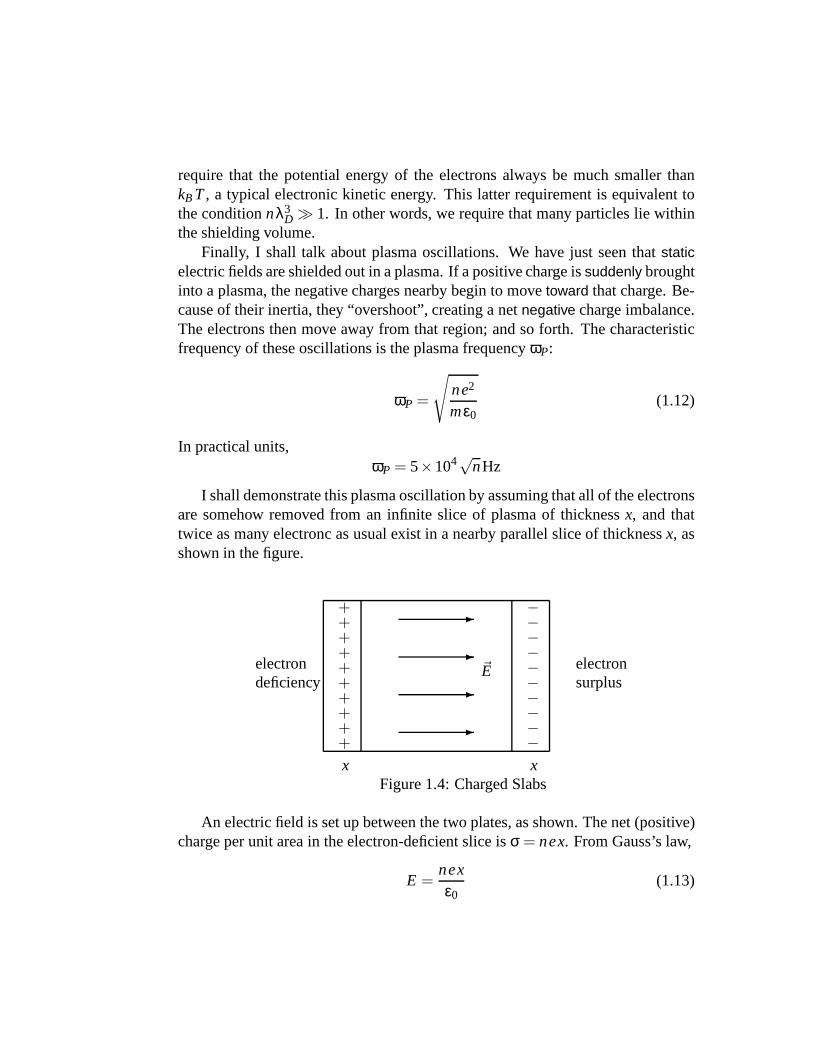
I shall demonstrate this plasma oscillation by assuming that all of the electronsare somehow removed from an infinite slice of plasma of thicknessx, and thattwice as many electronc as usual exist in a nearby parallel slice of thicknessx, asshown in the figure.
electrondeficiency
++++++++++
x
-
-
-
-
~E electronsurplus
−−−−−−−−−−
xFigure 1.4: Charged Slabs
An electric field is set up between the two plates, as shown. The net (positive)charge per unit area in the electron-deficient slice isσ = nex. From Gauss’s law,
E =nexε0
(1.13)
The electric field acts on the electrons in the intermediate region, causing them tomove to the left, and causing the slice thickness to decrease. (The acceleration ofeach electron is ¨x, in fact.) Thus, we obtain from Newton’s second law that
mx = −eE= −ne2
ε0x (1.14)
Thus,x(t) = x0 cos(ωP t +δ), so that the charge imbalance oscillates with (angu-lar) frequencyωP.
The particles in a plasma make collisions with one another – the more densethe plasma, the more frequent the collisions. Letν be the collision frequency, andτ = 1/ν the time between collisions. For the plasma state we requireωPτ≫ 1. Asa consequence, it is improbable for the electrons to collideduring a single plasmaoscillation. Thus, the plasma oscillations arenot merely damped out because ofinterparticle collisions. The electrons undergo these oscillations without any realcollisional damping, and such oscillations are characteristic of the plasma state.You will hear more about them.
A magnetic field plays an absolutely basic role in plasma physics; it penetratesthe plasma, even though the electric field does not. I shall briefly review themotion of a charged particle in a uniform~B field. The particle experiences theLorentz force,
~F = q~v×~B
By Newton’s second law, a charged particle moves with constant speed in thedirection parallel to~B, and moves in a uniform circular orbit in the plane perpen-dicular to~B. If v⊥ is the particle speed in the circle andr⊥ is the radius of thecircular orbit, then
qv⊥B = force= mass×acceleration=mv2
⊥r⊥
(1.15)
The particle moves in a circular orbit withcyclotron frequency
ω = v⊥/r⊥ = qB/m
The radius of the circular orbit,Larmor radius
r⊥ = mv⊥/(qB)
depends on the initial speed of the particle in the plane perpendicular to~B. Thecomposite motion of the charged particle is a helical spiralmotion along one ofthe lines of magnetic induction. Oppositely charged particles spiral around thefield line in the opposite sense.
Chapter 2
Single Particle Dynamics
2.1 Introduction
This lecture deals exclusively with the motions of a single charged particle inexternal fields, which may be electrical, magnetic, or gravitational in character.The motions of charged particles in external fields are the full story in cyclotrons,synchrotrons, and linear accelerators – the mving chargesthemselves producenegligibly small fields. The charged particle beams in such devicesaren’t plasmas,since collective effects don’t matter. In fact, nobody knows how to build high-current accelerators in which collective (space charge) effects are large – this isa verycostly limitation of accelerator technology. In a plasma, collective effectsoccur and are likely to be important. For some purposes, we may treat plasma asa collection of individual particles, and sometimes we musthandle the plasma asa continuous fluid.
The Lorentz force,~F = q~v×~B, causes a charged particle (chargeq, massm)to spiral around a line of force in auniform magnetic field. In the plane perpendic-ular to the field, the Larmor radiusr⊥ is determined by the initial transverse speedv⊥ by the relation
r⊥ =mv⊥qB
=
√2mE⊥qB
(2.1)
with the transverse kinetic energyE⊥ = mv2⊥/2. In practical units (B in Gauss,
E⊥ in electron Volts),
r⊥ = 3.37√
E⊥/Bcm
13
2.2 Orbit Theory
In the branch of accelerator (plasma) physics known asorbit theory, one assumesthat there is present a magnetic field~B that isapproximately uniform over a particleorbit, so that, to a first approximation, the charged particles spiral around fieldlines. The charged particles are, however,slightly affected by one or more of thefollowing small perturbative contributions:
• A small (time-independent) electric or gravitational field.
• A slight non-uniformity in the magnetic field, with its magnitude (|~B|)changing with position).
• A slight curvature of the lines of force of~B.
2.3 Drift of Guiding Center
As a consequence lf any of these small sources of perturbation, theguiding cen-ters of the particle cyclotron orbits experiencedrifts. These guiding center driftsarenot negligible. even though they come from small perturbations, because theyoften have a large cumulative effect over a long time. It is anexcellent approx-imation to think in terms of guiding center drifts with a distanceℓ, over whichnon-uniformities or small perturbations are important, asvery large in compari-son with the Larmor radiusr⊥; (ℓ ≫ r⊥).
We need consider only forces in the plane perpendicular to the uniform~B field– those parallel to~B simply accelerate the particle along~B, and do not affect thetransverse motion. Also, note that in apure magnetic field – be it non-uniform,curved, or whatever – the Lorentz force does no work on the particle:
~v ·~F = q~v · (~v×~B) = 0
Consequently, the mechanical energy of the particle does not change.The simplest case to illustrate guiding center drift is thatof a constant force
~F in plane perpendicular to a uniform magnetic induction~B. Let the force act inthex-direction, with the~B field in thez-direction. The mechanical energy of thesystem,12mv2
⊥−F x, is a constant of the motion. As a consequence, the presenceof the force~F perturbs the circular Larmor orbit; there are greater speeds, andconsequently larger radii of curvature (see Eq.(1)) forx > 0 than forx < 0,
~v�
Figure 2.1: Drift of Guiding Center
As a consequence, for counterclockwise circulation there is an upward drift ofthe guiding center for a positive charge, as shown inFigure 2.1.
We can analyze this motion quantitatively using Newton’s second law:
md~vdt
= ~F +q~v ×~B (2.2)
for thex- andy-components:
mdvx
dt= F +qvyB
mdvy
dt= −qvxB (2.3)
or
dvx
dt=
qBm
(
vy +FqB
)
ddt
(
vy +FqB
)
=dvy
dt= −qB
mvx (2.4)
If we define a velocity~u =~v + F/(qB) y, Eqn. (4) represents uniform cir-cular motion with angular velocityω = qB/m for the velocity vector~u. As aconsequence, the composite motion is circular motion with angular velocityω,
with respect to a guiding center that is drifting downward with speedF/(qB).Consequently, the drift velocity of the guiding center is
~vD = − jFqB
=1
qB2~F ×~B (2.5)
If the force~F is produced by a uniform electric field~E , then~F = q~E and
~vD =~E ×~B
B2 (2.6)
Thus, in a uniform electric field, all charged particles experience an~E ×~B drift,which is independent of the magnitude or sign of their charge, or their mass.
-�
-~E
⊙ ~B
Positive NegativeFigure 2.3: Drift of Positive and Negative Charge
We shall discuss several other circumstances in which thereare guiding centerdrifts in response to small perturbations to a uniform~B field. There is a systematicprocedure for analyzing such perturbations, which consists of (i) computing theaverageresidual force on a charged particle as it moves across a circular Larmororbit, and (ii) using Eq.(5) to compute the drift speed. We illustrate this procedurein discussingGradient ~B Drift.
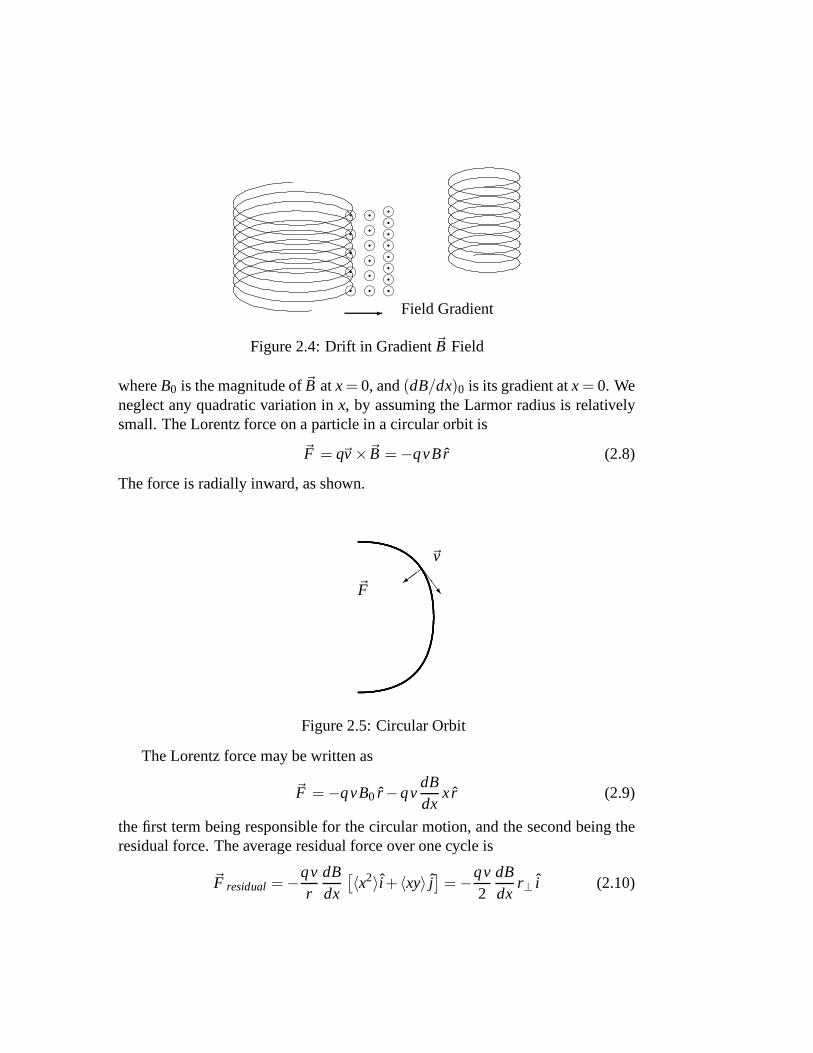
Let us assume that the~B field has fixed direction, with the magnitude increas-ing as one moves transverse to~B, to the left as shown inFigure 2.4. The Larmorradius,r⊥ = mv⊥/(qB), varies inversely toB. Thus, the left half of the orbitshould have a larger radius than the right half, as shown. Positive charges shoulddrift upward and negative charges should drift downward, asshown inFigure 2.4.
We shall compute the drift speed for positive charges. The magnetic inductionis assumed to vary linearly withx:
~B =
[
B0+xdBdx
]
z (2.7)
⊙⊙⊙⊙⊙
⊙⊙⊙⊙⊙⊙
⊙⊙⊙⊙⊙⊙⊙⊙
- Field Gradient
Figure 2.4: Drift in Gradient~B Field
whereB0 is the magnitude of~B atx= 0, and(dB/dx)0 is its gradient atx= 0. Weneglect any quadratic variation inx, by assuming the Larmor radius is relativelysmall. The Lorentz force on a particle in a circular orbit is
~F = q~v×~B = −qvBr (2.8)
The force is radially inward, as shown.
SSw
��=
~v
~F
Figure 2.5: Circular Orbit
The Lorentz force may be written as
~F = −qvB0 r −qvdBdx
xr (2.9)
the first term being responsible for the circular motion, andthe second being theresidual force. The average residual force over one cycle is
~F residual = −qvr
dBdx
[
〈x2〉i + 〈xy〉 j]
= −qv2
dBdx
r⊥ i (2.10)
since by symmetry〈xy〉 = 0 and〈x2〉 = 12r2
⊥. We use (2.10) in Eq. (2.5) to obtainthe drift speed
~vD =qV2
dBdx
j (2.11)
In general
~vD = ±qv⊥2B2 (~B×grad~B) (2.12)
with the± signs taken for positive (negative) particles.An additional source of charged particle drift is the curvature of magnetic field
lines. We shall discuss the case in which the magnetic field isof constant mag-nitude, with the field lines curved. A charged particle spirals around a particularfield line, as shown:
~R0
��
��
��
��
��
���
~B
Figure 2.6: Spiral around Field Line
If the radius of curvature of the field line (approximately circular) is~R0, theguiding center follows a spiral around the field line, as shown. The motion ofthe charged particle is most conveniently analyzed in a non-inertial coordinatesystem with the guiding center at the origin. In that system,the charged particleexperiences an inertial centrifugal force
~F =mv‖R2
0
~R0 (2.13)
with v‖ the speed parallel to the field lines. Thus, the curvature drift velocitycomes out to be
~vD =1
qB2~F ×~B =
mv2‖
qB2~R0×~B (2.14)
Remark: It is impossible to draw field lines for a~B-field that are curved, withouthaving |~B| to change, as well. Consequently, field gradients arealways presentwhenever the magnetic field lines are curved; we discuss themseparately for thesake of simplicity. As an example, let us consider a simple toroidal field. If a totalcurrent is distributed uniformly and without “twist” on thesurface of the torus,the magnetic induction has only a polar component
B0 =µ0 I
2πR0(2.15)
whereR0 is the radius of curvature of the field line, The field gradientis
grad|~B| = −µ0 I2π
~R0
R20
and the gradB drift is
~V D = ±v⊥ r⊥2
~R0×~B
R20B
=mv2
⊥2qB
~R0×~B
R20B
(2.16)
The overall drift for this toroidal field is
~vD =mq
~R0×~B
R20B2
(
V2+v2⊥/2
)
(2.17)
2.4 Adiabatic Drift
A particle in a uniform magnetic field spirals along a field line. If the field isslightly non-uniform, the particle either slowly drifts orspirals into regions ofspace that have different magnetic fields. Under such drifts, the radius of gyrationof the orbit changes sufficiently slowly, and there are certain adiabatic invariantsassociated with the orbit, which do not change. One such adiabatic invariant is theangular momentum action.
∮
L‖dθ = 2πL‖
the integral of the component of angular momentum about~B, taken over onegyration. Thus, the angular momentum component taken aboutthe guiding center,and parallel to the field, does not change.
L‖ = mv⊥ r⊥ =mv2
⊥ω
= mv2⊥
meB
=m2v2
⊥eB
=2meE⊥B
(2.18)
The quantityE⊥ = mv2⊥/2, the transverse kinetic energy, is the contribution to
the kinetic energy from transverse motion. From (2.18), we see that as the particlespirals or drifts into a region of increasing magnetic field,the transverse speedv⊥and energyE⊥ both increase.
As a particle of chargeemoves with angular frequencyω in a circular orbit ofradiusr⊥, one may define an average currentI = e/T = eω/(2π), and a magneticmoment
µ = current×area=eω2π
πr2⊥
=eω2
r2⊥ =
ev2⊥2ω
=ev2⊥
2meB
=E⊥B
(2.19)
Consequently, the magnetic moment of the “current loop” is also an adiabaticinvarian. The flux of magnetic field through the loop,π r2
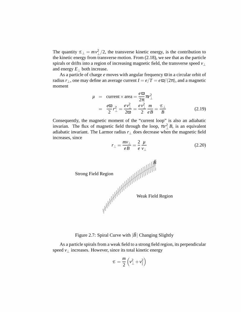
⊥B, is an equivalentadiabatic invariant. The Larmor radiusr⊥ does decrease when the magnetic fieldincreases, since
As a particle spirals from a weak field to a strong field region,its perpendicularspeedv⊥ increases. However, since its total kinetic energy
E =m2
(
v2⊥ +v2
‖
)
must remain fixed, the longitudinal speedv‖ must decrease. If the particle spiralsalong a field line to a point at whichv‖ is zero, the particle is reflected.
2.5 Magnetic Mirror
These features form the basis for a plasma confinement systemknown as aMag-netic Mirror. (SeeFigure 2.8.) Plasma is trapped in the central weak field region,being reflected as it enters the strong field region near the coils.
⊙ ⊙
⊗ ⊗
~B
coil coil
Figure 2.8: Magnetic Mirror
The magnetic mirror is not a perfect confining device for plasma, since ifv⊥is very small to begin with, it remains small and thusv‖ never gets small. The netresult is escape for that charged particle. In fact, ifv⊥ has the valuev0⊥ has thevalue in the weak field region, its value in the strong field region is
v⊥max=Bmax
B0v0⊥ (2.21)
If plasma goes past the point of maximum field,v‖ ≥ 0 at this point, and
v2⊥max≤ v2
0‖ +v20⊥ (2.22)
We thus obtain
1+
(
v0‖v0⊥
)2
≥ Bmax
B0(2.23)
as a condition for escape of plasma.
If we define the mirror ratio
Bmax
B0= sin2 θ (2.24)
the condition for escape may be written as
v0⊥v0‖
≤ tanθ (2.25)
��
�
JJ
JJ
JJ
JJ
JJ
θ
loss cone
field line-
Figure 2.9: Loss Cone
In other words, all particles within theloss cone escape. As a consequence,the mirror-confined plasma is definitelynon-isotropic.
Electrons and ions are equally well confined in a magnetic mirror, althoughelectrons are more likely to escape through collisions. Since it is hard for particlesto escape from a magnetic mirror, it is equally hard to get them inside the magneticmirror in the first place. Usually they are put inside the bottle with aninjector. Iftheir motion were perfectly adiabatic, they would come backto hit the injector, soit is just as well for their motion to be slightly non-adiabatic!
As a charged particle spirals along a field line, and is reflected ata andb by thestrong fields, it in general experiences transverse drifts because of external fields,etc. An adiabatic invariant for these drifts is the “longitudinal invariant”,
J =∫ b
av‖ds (2.26)
wheres is the path length along the guiding center that lies along a field line.If drifts occur over a time scale that is long in comparison with the period ofoscillation froma to b, thenJ remains an adiabatic invariant.
We may apply these concepts of drift, adiabatic invariants and such to themotion of charged particles in the earth’s magnetic field. The earth is like a giantbar magnet with magnetic dipole momentM = 8×1025 Gauss cm3. (TheNorthpole of the earth is closest to thesouth pole of the magnet.) At the equator on theearth’s surface (R= 6.4×10⁶ m).
B≈ MR3 = 0.2 Gauss (2.27)
As one goes along a field line toward the poles, the magnetic field increases inmagnitude. Particles in theVan Allen belts are trapped in the earth’s magneticfield; they executelatitude oscillations about the equator.1 Their motion is simpleharmonic, with angular frequency
ωlat =3ω√
2
r⊥R
(2.28)
wherer⊥ is the Larmor radius andω the cyclotron frequency at the equation;R isthe distance to the center of the earth.
There is also alongitude drift because of field gradients:
vgrad =ω r2
⊥2B
·gradB =3ω r2
⊥2R
(2.29)
The angular frequency of longitude drift is
ωlong =vgrad
R=
3ω2
R2
r2⊥
(2.30)
For 10 keV electrons atR = 3× 10⁷ m (five earth radii) andr⊥ = 103 m,the period of latitude oscillation is about 1.4 sec, and the longitude period (timenecessary to drift around the earth) is 7×10⁴ sec. The earth’s magnetic field is3×10−3 Gauss, and the cyclotron frequency isν = 2500 Hz.
1Particles within the loss cone may well travel all the way to the earth’s surface, causing theAurora Borealis (Northern Lights) in polar regions.
Chapter 3
Plasmas as Fluids
3.1 Introduction
For 80% or so of the applications in plasma physics, it is sufficient to treat theplasma as a fluid of charged particles, in which electromagnetic forces are takeninto account. The plasma fluid equations are a relatively simple modification ofthe Navier-Stokes equations; they must be supplemented by Maxwell’s equationsof electromagnetism, and the requirements of conservationof mass and charge.
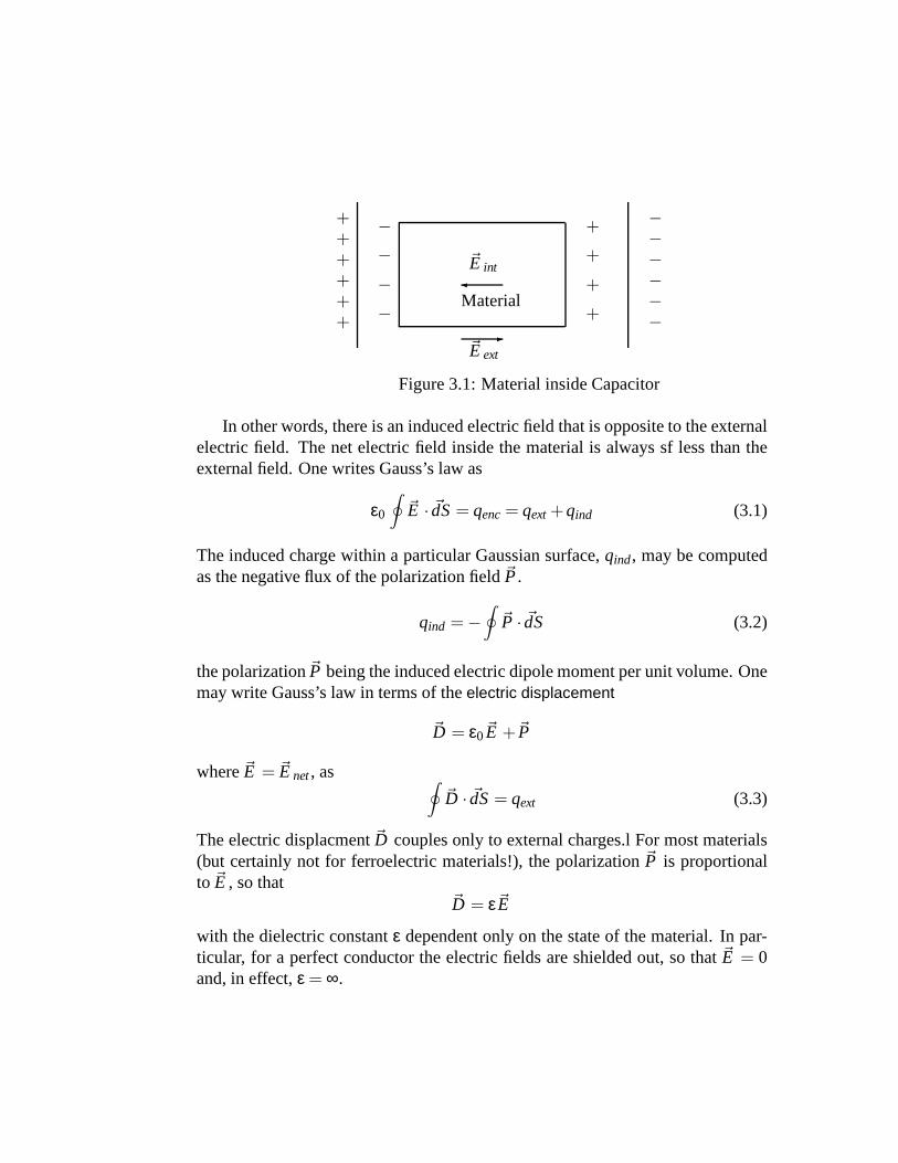
Before discussing plasma as a fluid, I shall discuss the bulk properties ofplasma (considered as a material medium) in electric or magnetic fields, and shallcompare these bulk properties with the properties of ordinary matter. We beginby considering an external electric field, set up by placing acharge on externalcapacitor plates. When a slab of matter lies between the capacitor plates, the ef-fect of the external electric field~E ext is to polarize the charges in the slab, so thatopposite charges are induced on the faces of the slab nearestto to a respectivecapacitor plate, as shown.
25
++++++
−−−−
+
+
+
+
−−−−−−
-~E ext
�~E int
Material
Figure 3.1: Material inside Capacitor
In other words, there is an induced electric field that is opposite to the externalelectric field. The net electric field inside the material is always sf less than theexternal field. One writes Gauss’s law as
ε0
∮
~E · ~dS= qenc= qext+qind (3.1)
The induced charge within a particular Gaussian surface,qind, may be computedas the negative flux of the polarization field~P.
qind = −∮
~P · ~dS (3.2)
the polarization~P being the induced electric dipole moment per unit volume. Onemay write Gauss’s law in terms of theelectric displacement
~D = ε0~E +~P
where~E = ~E net, as∮
~D · ~dS= qext (3.3)
The electric displacment~D couples only to external charges.l For most materials(but certainly not for ferroelectric materials!), the polarization~P is proportionalto ~E , so that
~D = ε~E
with the dielectric constantε dependent only on the state of the material. In par-ticular, for a perfect conductor the electric fields are shielded out, so that~E = 0and, in effect,ε = ∞.
A plasma is like a perfect conductor, in that it shields out static electric fields;the charges within the plasma rearrange themselves so thaatthe ~E -field is zeroexcept within approximately one Debye length of the edges ofthe plasma. De-bye shielding is effective only if there is no magnetic field in the plasma; in thepresence of a~B field the shielding is less complete, as we shall see.
If a magnetic induction~B is present, the charged particles spiral around thefield lines with frequency
ωc = qB/m
If, in addition, atransverse electric field
~E exp(iωt)
is present, the charged particles undergo apolarization drift in the direction of thechange of ~E .
If ω the frequency of variation of~E , is small in comparison with the cyclotronfrequencyωc, we get a drift velocity
~vD = ± 1ωcB
d~Edt
= ± mqB2
d~Edt
(3.4)
Note: the drift speed is roughly±iωE/ωcB. With this drift speed in the directionof the transverse electric field, one may associate apolarization current (flow ofelectric charge) with the motion of ions and electrons
~J = ne(
~V ions−~velec
)
=nB2 (me+mi)
d~Edt
=ρB2
d~Edt
(3.5)
whereρ = n(me+mi)
is the mass density of the plasma. This current is associatedwith the drift of elec-tric charges, and the locations of the electric charges mustbe taken into accountin Gauss’s law, Eq. (3.1). From the requirement of conservation of the flow ofcharge, applied to a Gaussian surface, it follows that
− ddt
qind =
∮
~J · ~dS=ρB2
ddt
∮
~E ind · ~dS (3.6)
Thus, for low frequency time-dependent electric fields we have
qind = − ρB2
∮
~E · ~dS (3.7)
On comparing (3.7) with (3.2) and the definition of the dielectric constantε andthe electric displacement, we obtain
ε = ε0+ρb2 (3.8)
For a rather diffuse plasma with a stron electric field,n = 1010 partiles per cubiccentimeter andB = 1 kG,ε/ε0 = 200, and in generalε increases with an increasein density and a decrease in magnetic field strength. Therefore, AC fields arefairly well shielded out by a plasma. The expression (3.8) isvalid for transverselow-frequency only; in general the dielectric constant hasrather complicated de-pendence on direction and frequency.
We shall now discuss the bulk properties of plasma, in contrast to those ofordinary matter. Ampère’s law for ordinary matter has the form
1µ0
∮
~B · ~dℓ = ienc= iext+ i ind (3.9)
where the induced current is related to themagnetization ~M (magnetic dipolemoment per unit volume) by the relation
i ind = −∮
~M · ~dℓ (3.10)
The magnetic field~H is defined by the relation~B = µ0(~H + ~M ), where theH-fieldcouples only toexternal currents:
∮
~H · ~dℓ = iext (3.11)
For a material medium we define the magnetic permeabilityµ by the relation
~B = µ~H
A plasma must be considered as a diamagnetic medium,µ< µ0, since the magneticinduction~B in generated by the spiraling of the charges is opposite in direction tothe external induction~Bext. The magnetic dipole moment of one spiraling particleis
µ= mv2⊥/(2B)
see Eq. (2.19). The magnetization is obtained by multiplying the average value ofµ by n, the number of particles per unit volume:
M =mnv20⊥
2B(3.12)
for each species of charged particle in the plasma. Since themagnetization variesinversely as the magnetic induction, there is usually no advantage in treating theplasma as a magnetic medium. That is, one usuallly works directly with Ampère’slaw in the form (9), rather than the form (11) that couples only to external currents.
3.2 Fluid Equations
In the fluid approximation, one treats the positive ions, thenegatively chargedelectons, and the neutral particleseach as fluid components. The plasma is amixed three-component fluid. The fluid equations include the effect of collisionsand interactions of the fluid components, but do not take proper account of mo-tions of the individual particles. In an ordinary fluid, the particles undergo fre-quent collisions, and these collisions justify the “fluid average” approximation. Inplasma, the particles collide somewhat infrequently, but the magnetic field pro-duces a similar averaging effect. That is, the magnetic fieldconstrains thetrans-verse motion of the charged particles, and thereby helps in the statistical averagingprocess. The fluid approximation is less valid in regard tolongitudinal motions inplasma.
To illustrate the rather similar effects of collisions and the magnetic field, letus discuss the flow of curent in response to an electric field~E . In a copper wire,the electrons have drift velocities
~vd = µ~E
where the electron mobility is determined by the frequency of collisions in a metal.In plasma, there is a drift velocity
~vd = ~E ×~B/B2
In the fluid approximation, one assumes that each infitimesimal clump of fluidmoves without breaking up, so that one may associate a velocity with each clumpof fluid. (We ignore the fact that the individual molecules inthe clump have differ-ent velocities.) The fluid equations of motion for the plasma, which are analogousto the Navier-Stokes fluid equations, are obtained by applying Newton’s secondlaw to an infinitesimal clump of fluid of massm and chargeq:
md~vdt
= q(
~E +~v ×~B)
+collisional forces (3.13)
The termd~V /dt, which is the acceleration of a particular clump of fluid, isnotsimply the rate at which the velocity is changing at aparticular point in space. Thisterm is somewhat inconvenient both to measure and to deal with analytically, sinceone must follow each fluid clump to determine it. Instead, it is conventional tomake use of the velocity field~u(~r , t), which gives the velocity of fluid at position~r and timet. The fluid clumps experience accelerations when the velocity field~uis nonuniform in spaceor in time; in fact the accelerationd~v/dt is the so-calledconvective time derivative of the velocity field,D~u/Dt:
D~uDt
=∂~u∂t
+∂~u∂x
dxdt
+∂~u∂y
dydt
+∂~u∂z
dzdt
=∂~u∂t
+∂~u∂x
vx +∂~u∂y
vy +∂~u∂z
vz (3.14)
Remark: The convective time derivative not just the ordinary time derivative of afield. Your house may be losing heat (nonzero convective derivative of tempera-ture with respect to time) even though the thermometer reading on the thermostatdoes not change.
Let us apply Eq. (13) to an infinitesimal volumedV, containingndV chargedparticles, and divide it bydV. We obtain
mnD~uDt
= qn(
~E +~v×~B)
+pressure force per unit volume (3.15)
The pressure force in a fluid can be computed for a cubic fluid element, withpressurep1 (down) on the top face and pressurep2 (up) on the bottom face. Thebouyant force (up) is
(p2− p1)A = (p2− p1)V/h
Consequently, the force per unit volume on a small cube is equal to−dp/dx, thenegative of the pressure gradient.
The fluid equaiton (15) must be supplemented by the equation of state of theplasma – one must know how the pressure of plasma changes withits density.A dilute plasma in thermal equilibrium, like a dilute gas of neutral particles or adilute solute, obeys the perfect gas law
pV = N kBT or p = nkBT
As with the gas or the solute, there are two very common ways inwhich thepressure changes with density:
1. Isothermal changes – the chnages in density are sufficiently gradual that thesystem remains in thermal equilibrium at temperatureT, sop is proportionalto ρ.
2. Adiabatic changes – changes in the state of the plasma often occur overtimes too short for thermal equilibrium to be established; such changes canbe treated as adiabatic (sudden).
For adiabatic changes in the state of an ideal gas,pVγ is an invariant. Theplasma may usually be treated for such purposes as a one-dimensional gas ofpoint particles, so thatγ = 3. the appropriate pressure-density relation is
p = cργ (3.16)
The pressure increases with density for adiabatic, as well as for isothermal, pro-cesses.
Remark: The plasma will often be in thermal equilibrium separatelyfor lon-gitudinal and transverse motions, with different temperatures. That is, the plasmamy have time to establish separate thermal equilibrium withrespect to longitudinaland transverse motions, but there maynot be enough time for these independentdegrees of freedom to come into mutual equilibrium. The Maxwell-Boltzmanndistribution of speeds would be non-isotropic in such cases, with different “tem-peratures” for transverse and longitudinal directions.
Let us now discuss the fluid motions of plasma in external electric and mag-netic field. We begin by talking abouttransverse motions, perpendicular to~B.The fluid equation is
mnD~uDt
= qn
(
~E +~u×~B +1
qngradp
)
(3.17)
The structure of this equation for transverse motions is very similar to thosesingle-particle equations discussed inChapter 2. The term~u ×~B causes Larmorgyration of the fluid, whereas the other two terms induce fluiddrifts. The secondterm gives rise to an “~E ×~B drift” in the fluid, with drift speed
~vD =1B2
~E ×~B (3.18)
and the third term produces a “pressure gradient drift”, or “diamagnetic drift” withspeed
~vD − 1qmB2 gradp×~B (3.19)
This ~E ×~B drift is identical with that encountered in the single particle case. Tounderstand the physical basis for diamagnetic drifts, consider a plasma in whichthe pressure gradient goes to the left and the~B field points out of the paper. Theplasma is more tenuous to the right, and fewer particles are moving in cyclotronorbits. In the strip shown, more particles enter from the left, and move downward,than enter from the right to move upward. Therefore, there isa new downwarddrift of fluid in the strip. (SeeFigure 3.2.)
In practical units, for isothermal drifts of electrons,
~vD = 108 kBTLB
cm/sec (3.20)
whereT is the transverse electron temperature, withkBT in electron Volts,B is themagnetic induction in Gauss, andL is the length scale (in cm) over which densitychanges occur in the plasma.
GradientB drifts and curvature drifts do not occur in the fluid picture.Thesedrifts are absent here, since the magnetic induction does not work on charged par-ticles, and the presence or absence of a~B field does not affect the Maxwelliandistribution of speeds. In other words, although the guiding centers of the in-dividual particles do experience drifts, these drifts are presumably cancelled outby collective fluid effects. The fluid picture and the single particle picture aresomewhat contradictory on the matter of these drifts.
For fluid drifts in the direction parallel to the~B field (thez-direction) the fluidequation for the more mobile electons becomes
mnD~uz
Dt= qnEz−
dpdz
(3.21)
Because the electrons are light, they very quickly rearrange themselves so thatthe pressure gradient term in (3.21) cancels out the external electric field. Fur-thermore, such rearrangements occur so quickly that thermal equilibrium is estab-lished. Thus,
qnEz =dpdz
=∫
kB Tdndz
(3.22)
We can relate the left side of Eq. (3.22) to the electric potential φ by writing it as
(−e)n(−dφ/dz) = en(dφ)(dz)
The number density of the electrons is therefore
n(z) = n0exp[eφ
kBT] (3.23)
The electrons are attracted to the regions of high electric potential, and pushedawan from the regions of low potential; the pressure gradients of the electronscancel out the external electric fields.
dense plasma ⊙ ⊙ ⊙ ⊙ ⊙ tenuous plasma
pressure gradient�???
matter flow
�?�?�?�?�?�?�?�?
�?�?�?�?�?
�?�?
�?
�?
Figure 3.2: Diamagnetic Drift
Chapter 4
Waves in Plasmas
4.1 Introduction
We shall be concerned with certain disturbances from equilibrium in a plasmapropagate in space as time passes. These disturbances are wavelike, and similarin spirit to sound waves, water waves, earthquake waves, andelectromagneticwaves. Before discussing various distinct types of waves inplasma, we brieflyreview wave phenomena in general. For simplicity, we shall discuss waves inone-dimensional space – the generalization to three-dimensional space is directand obvious to those readers with the appropriate background.
Let f (x, t) be the “wave disturbance” at positionx and timet. ( f might be thedisplacement of particles from equilibrium, or the magnitude of the electric field,in a physical situation.) For a plane wavef is a sinusoidally varying functionthroughout space and time:
f (x, t) = Re(
f0eiφ ei(kx−ωt))
= f0 cos(kx−ω t +φ) (4.1)
where the following real variables appear in (4.1):
• f0: wave amplitude
• φ: phase of wave (atx = 0 = t)
• k: wave number
• ω: angular frequency
35
Plane waves are unphysical, in that they persist throughoutall space and time;we discuss them merely because they are the simplest solutions of the wave equa-tions. Real waves, or “wave packets” are localized in space;we may representthem as superpositions of plane waves.
We introduce the concept of superposition by taking the sum of two wave dis-turbances of equal amplitudef0 and almost the same wave number and frequency:[(ω1,k1) and(ω2,k2), respectively.] We obtain the net disturbance
f0cos(k1x−ω1t +φ1)+ f0cos(k2x−ω2t +φ2) = (4.2)
2 f0cos
[
k1 +k2
2x− ω1 +ω2
2+
φ1+φ2
2
]
cos
[
k1−k2
2x− ω1−ω2
2+
φ1−φ2
2
]
The appearance of two separate cosines on the right side is characteristic of su-perposition. The first factor represents thecarrier wave. That factor remains fixedwhenever
kx−ωt
does not change, wherek is the average wave number andω is the average angularfrequency. In other words, the carrier wave propagates withvelocity equal to thephase velocity
vP = ω/k (4.3)
The second cosine factor represents the propagation of energy and information inthe wave; it remains fixed whenever
∆kx−∆ω t
does not change, with∆k the spread in wave number and∆ω the angular frequencyspread. Consequently, the energy of the wave propagates with the group velocity
vg =∆ω∆k
→ dωdk
(4.4)
We shall use Maxwell’s equations and the fluid equations to identify various typesof disturbances propagating in plasma, and to obtain thedispersion formula to giveangular frequencyω as a function of the wave numberk for these various types ofplasma waves.
As discussed in Chapter I, a charge imbalance in a plasma setsup an electricfield, and the charges subsequently oscillate about their equilibrium positions withthe plasma frequency
ωP =
√
ne2
ε0≈ 9000
√n rad/sec (4.5)
wheren is the number of particles per cubic centimeter in the last term. Theplasma oscillation is the key to propagation of waves in plasma, in the same sensethat molecular motion is the key to propagation of sound in matter. However, theoscillations do not set up a propagating distrubance in an infinite plasma, sinceωP
is independent ofk, and the corresponding group velocityvg = dω/dk is zero.1
4.2 Electron Plasma Waves
We shall first discuss electron plasma waves, which are electrostatic waves thatpropagate in a plasma with no external magnetic field. A disturbance propages be-cause of the thermal motion of the electrons; one gets a condensation-rarefactionelectron density wave in the plasma.2
To discuss electron plasma waves in detail, we write the electron number den-sity n(x, t) as
n(x, t) = n0+n1(x, t) (4.6)
wheren0 is the uniform equilibrium electron density3 andn1 represents the prop-agating wave density. The fluid equation for the electrons relates the convectivederivative of the velocity field~v to the electric field~E and the pressure gradient:
mnD~vDt
= −en~E −gradp (4.7)
We assume thatn1, the deviation from uniform electron density, and~v, the velocityfield of the electrons, are small, and keep only first order terms to obtain
mn0DVx
Dt= −en0Ex−
dpdx
(4.8)
If we assume the wave propagates adiabatically, the pressure gradient may be re-placed by 3kBT dn1/dx. Let us taken1 andVx to have the space-time dependenceof a plane wave:
n1(x, t) = n1ei(kx−ωt) vx(x, t)−vxei(kx−ωt) (4.9)
We put (4.9) into (4.8) to obtain
imn0ωvx = en0Ex +3i kBT n1 (4.10)
1In an infinite plasma, there is a propagating disturbance because offringing fields – but nevermind that.
2If the electrons had no thermal motion, the usual localized plasma oscillation would occur.3We are pretending in this chapter that particles are of uniform density in the plasma!
The fluid equation (4.8) must be supplemented by Gauss’s law and the equationof continuity, or law of conservation of the flow of electrons, in determining thedispersion relationω(k) for these electron plasma waves. We discuss both of themin terms of a closed transverse cylindrical surface of cross-sectional areaA, withfaces at longitudinal faces at 0 andx, as shown inFigure 4.1.
-
�
�
�
�
�
�
�
�0 x
Figure 4.1: Cylindrical Gaussian Surface
By symmetry, the electric field has anx-component independent ofy andz, sothat the flux of the electic field is
(Ex(x)−Ex(0))A
The net charge density inside the cylinder is−en1. (We have assumed that theplasma in bulk is electrically neutral, with the ion charge density to cancel out thebackground electric charge density−en0. Gauss’s law yields the relation
ε0(Ex(x)−Ex(0))A = −eA∫ x
)dxn1
or
ε0dEx
dx= −nie (4.11)
The law of conservation of mass requires that the negative time derivative of theamount of mass inside equals the flux of mass through the surface. There is noflux through the lateral surface, so that
− ddt
∫ x
0(nmA)dx= (n(x)v(x)−n(0)v(0)) mA (4.12)
We divide bymAand differentiate with respect tox to obtain
−dndx
=ddx
(nvx) (4.13)
or, to first order,dn1
dx= −n0
dvx
dx(4.14)
We use the plane wave expression (4.9) in (4.11) and (4.14), as well as a similarexpression for the electric fieldEx, to obtain
ikε0Ex = −n1e
iωn1 = ikn0vx (4.15)
We then use (4.15) to eliminateEx andn1 in the fluid equation (4.10).
imωvx = en0−eikε0
kn0vx
ω+3kBT(ik)
kn0vx
ω(4.16)
or
ω2 =n0e2
mε0+
3kBTm
k2 = ω2P +
3kBTm
k2 (4.17)
The dispersion curve ofω versusk is one branch of a hyperbola.For the group velocityvg = dω/dk we have
vg =3kBT
mkω
≤√
3kBTm
= vth (4.18)
It is always less than the thermal speed, and approaches it at large wave num-ber. At small wave number, the pressure gradient term in (4.8) is small, and thegroup velocity is small in comparison with the thermal speed. By contrast, thephase velocity is always larger than the thermal speed, and becomes infinite askapproaches zero.
The experiments of Looney and Brown (1954) established the existence ofelectron plasma waves.
The discussion of electron plasma waves is similar to that ofsound waves in anideal gas, except that the electric field plays a role. We recover the expression fortransmission of sound waves by making these changes in the above expression:
• Since the atoms of the gas are neutral, we set the chargee and the electricfield Ex equal to zero.
• The factor of 3kBT in (4.10), (4.16), and (4.17) should be replaced byγkBT,whereγ is the ratio of specific heats for the gas in question.
The sound wave propagates because of atomic collisions, andthe dispersionrelation is
ωk
=
√
3kBTm
(4.19)
(Of course,m is the mass of the atom itself.)
4.3 Ion Acoustic Waves
Next we discussIon Acoustic Waves, which are the plasma physics version ofsound waves. These waves propagate because the more mobile electrons shieldout the ion electric field, but set up their own field to drive the ions in a tenuousplasma. These waves can be excited, even though the electrons and ions haveinfrequent collisions. The external magnetic field is zero for these waves.
The ion fluid equation has the form
M nD~v i
Dt= en,~E −gradp = −engradφ− γi kBTi gradn (4.20)
We have introduced the electrostatic potentialφ and assumed adiabatic changesin the ion state in obtaining this relation. We make theplasma approximation indiscussing ion waves; that is, we assume that the more mobileelectrons shield outthe electric field produced by the ions; so that the electron and ion densities areequal to one another and have the value
ni = ne = noexp
[
eφkBTe
]
(4.21)
whereφ is the electric potential at the point in question. If we assume the elec-trostatic energy to be small compared tokBTe, the ion density may be writtenas
ni = n0
(
1+eφ
kBTe
)
(4.22)
The uniform background density of electrons and ions isn0.Let us substitute plane wave forms forni ,~v, andφ into the fluid equation (4.20)
to obtain the first order equation
iωnovix = en0(ikφ)− γi kBTi(ikn1) (4.23)
Finally, we need the ion equation of continuity (4.13), which gives
iωn1 = ikn0vix (4.24)
We eliminaten1 andφ to obtain
iωM n0vix =ikn0vix
ωik(kBTe)+
kn0vix
ωik(γi kBTi) (4.25)
orω2
k2 =kBTe
M+ γi
kBTi
M(4.26)
In a practical context, the electron temperatureTe is often much larger than theion temperatureTi , so that the first term on the right dominates (4.24). In otherwords, the dominant mechanicsm for wave propagation is the residual electricfield produced by the thermal motion of electrons about equilibrium. The ionacoustic wave propagates because of the thermal agitation of the electrons (anisothermal process – the electrons have time to come to thermal equilibrium beforethe ions move) and the thermal agitation of ions (an adiabatic process).
Let us now turn to the discussion of electrostatic oscillations of a plasma in auniform magnetic field~B – in particular, we discuss the oscillations of electronsin the plane perpendicular to~B. Such oscillations are produced by two distinctphysical mechanisms:
• plasma oscillations of frequencyωP
• Larmor gyration of electrons in the magnetic field, of frequency
ωc = eB/m
The “upper hybrid frequency” for such oscillations isω, where
ω2 = ω2P +ω2
c =
(
ne2
mε0
)2
+
(
eBm
)2
(4.27)
The plasma frequency and the cyclotron frequency are of comparable magnitudesin a typical laboratory plasma. The frequency is greater than eitherωP or ωc,since the electron restoring force and the Lorentz force areadded to give the totalrestoring force, which is greater than each force separately.
The electromagnetic oscillations do not themselves propagate, becauseω isindependent of the wave numberk, but they and other plasma oscillations do pro-vide a mechanism for propagation of waves in plasma. We mention in passingone example of such a propagating wave: electrostatic ion acoustic waves, whichpropagate in the direction perpendicular to the external field ~B0, and are subjectto the dispersion relation4
ω2 =
(
eB0
m
)2
+k2 kB Te
m(4.28)
The ion cyclotron frequency plays the same role here as the electron plasma fre-quency in electron plasma waves; see Eq. (4.17).
4.4 Electromagnetic Waves in Plasma
Let us now turn the discussion to the propagation of electromagnetic waves inplasma. We begin with electromagnetic electron waves, withno external fields.The electrons in the plasma are accelerated by the electromagnetic field of theincident wave, and the electrons, in turn, produce~E and~B fields on their own thatmodify the form of the wave. The dispersion relation for these plasma waves is
ω2 =
(
ne2
mε0
)2
+c2k2 = ω2P +c2k2 (4.29)
Note that the group velocity of such waves,vg = c2k/ω, is alwaysless than thevelocity of light c, so that the presence of plasma in a region serves to reducethe speed of propagation of electromagnetic radiation. Note also that, sinceω isnot merely a linear function ofk, there is dispersion of a wave packet in plasma –components with different wave numbers propagate with different speeds. Finally,note that ifω is less than the plasma frequencyωP, the wave numberk must bepurely imaginary – such waves are exponentially damped in the plasma and cannotpropagate through it. As electromagnetic wave that comes toa region in space inwhich ω < ωP is, in general, reflected at the boundary. The physics is the sameas that oftotal internal reflection, the process by which light is transmitted throughlucite fibers, for example.
The earth’s ionosphere has a density of about 106 charged particles per cubiccentimeter, and the plasma frequency is about 107 Hz. Electromagnetic waves
4(We have neglected the ion temperature here.
of below that frequency (e. g., AM radio waves) are reflected by the ionosphere,whereas waves of higher frequency (FM and TV, for example) are transmittedthrough the ionosphere. One may communicate over great distances with shortwaves by making reflections off the earth’s ionosphere. On the other hand, com-munications with satellites in the ionosphere and beyond5 must employ electro-magnetic waves of higher frequency. Theplasma cutoff, or blackout of communi-cations of satellites upon re-entry through the earth’s atmosphere, is another man-ifestation of this attenuation of low-frequency electromagnetic waves in plasma.
We shall briefly mention electron electromagnetic waves in plasma with a uni-form magnetic field~B0. It is possible for waves to propagate in a direction perpen-dicular to~B0 – there are direction-dependent effects, just as for electromagneticwaves propagating in an anisotropic crystal. In addition, electromagnetic wavesalso propagate in a direction parallel to~B0. Because the electrons and ions in aplasma undergo Larmor gyration in the external magnetic field, there is a naturalasymmetry, so that left and right circularly polarized waves have different disper-sion relations. In particular, if we take the electrical conductivity of the plasmainto account, waves with one sense of polarization are attenuated over shorterdistances than those with the other sense. With~B0 = 0, waves are in generalattenuated rapidly because of the effect of conductivity. These readily transmit-ted waves are called “helicons” in solid state physics and “whistlers” in plasmaphysics.
When lightning flashes occur in the Southern hemisphere, a broad spectrum ofelectromagnetic radiation propagates along magnetic fieldlines (without substan-tial attenuation), coming back to earth in the Northern latitudes where the fieldlines return to the earth. The group velocity of these waves increases with fre-quency, so that the high frequency waves arrive first and th low frequency wavesarrive later. (These waves are readily converted into an audio signal by “super-heterodyning”.) The characteristic “chirp” or whistle of these signals (i. e., a shiftfrom high pitch to low pitch) gives these signals their name.Whistlers were firstdetected by primitive military shortwave communications in Normandy in WorldWar I.
5and with little green men in outer space via ESP
4.5 Alfvén Waves
Finally, we discuss low frequency ion electromagnetic waves in the presence ofan external magnetic field; in particular, we consider hydromagnetic waves, orAlfvén waves, which propagate parallel to~B0. The electron and ion motions liein the plane perpendicular to the wave number~k. The dispersion relation forelectromagnetic waves in a material medium with dielectricconstantε is
ω2
k2 =c2
ε/ε0(4.30)
We may adapt this formula to plasmas, takingε to be the transverse dielectricconstant in an external magnetic field~B0 for a plasma of densityρ. See Eq. (3.8).
ε = ε0+ρB2
0
(4.31)
In general,ε ≫ ε0, and one has approximately
ω2
k2 =c2 ε0B2
0
ρ≡ v2
A (4.32)
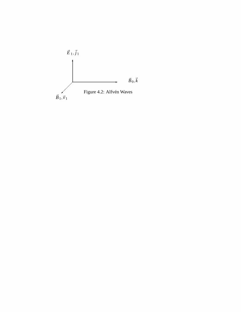
wherevA is the Alfvén velocity.The physical explanation of Alfvén waves is that a currentj1 is produced in
the direction of the induced electric field~E 1 of the electromagnetic waves, as aresult of Ohm’s Law. The elctrons and the ions experience a drift ~v1 = ~E 1×~B/B2
– this is just the~E ×~B drift. The currentj1 experiences a Lorentz force
~F = ~j 1×~B
which serves to cancel the~E ×~B drift, and produce oscillations. The transverseelectric and magnetic fields are related by Faraday’s Law:
E1 = ωB1 k
We mention that, among many other varieties of ion electromagnetic waves,there are magnetosonic waves, which are acoustic waves propagating perpendicu-lar to~B0. Compressions and rarefactions of plasma are produced by~E ×~B driftsalong the wave vector~k.
-
6
��
�
~B0,~k
~E 1,~j 1
~B1,~v1
Figure 4.2: Alfvén Waves
Chapter 5
Diffusion, Equilibrium, Stability
5.1 Introduction
We have been discussing plasma of uniform density up to now, but in actual labo-ratory practic plasmas are certainly not of uniform density. There is certain to bea net movement (diffusion) of particles from high-density regions to low-densityregions (e. g., to the walls). In laboratory confinement of plasma for the purposeof studying or inducing controlled thermonuclear reactions, the magnetic field isused to impede the process of diffusion in a weakly ionized plasma, in which therelevant equations are linear, and therefore simpler than in the strongly-ionizedcase.
The fluid equation for the charged particle velocity field is
mnD~vDt
= ±en, ~E −gradp−mnν~v (5.1)
The first two force terms come from electric fields and pressure gradients, whereasthe third is a collisional term. The parameterν is the collision frequency multi-plied by the fraction of momentum lost by a charged particle in an average col-lision. Let us apply this equation to a steady-state diffusional process, so that∂~v/dt = 0. Under the additional assumption that the diffusional velocity ~v issmall, we may set the convective derivativeD~v/Dt equal to 0. Finally, we assumethe diffusion to take place under isothermal conditions: gradp = −kBT gradn.One may then solve Eq. (5.1) for the velocity field:
~v =1
mnν
(
±en~E −kB T gradn)
= ± emν
~E − kBTmn
gradnn
(5.2)
47
The coefficient of~E is themobility µ of the charged particle, and the coeffient ofgradn in the second term is thecoefficient of diffusion D.
The particle flux at a point in space, which is defined as the number of particlespassing through a unit area per unit time, is~Γ = n~v. We thus have
~Γ = ±µn~E −Dgradn (5.3)
A particle flux can be independently produced as a result of anelectric field or adensity gradient. We have made the tacit assumption that diffusion is producedas a result ofrandom motions of the particles. However, since the motions inan external magnetic field are not random, the above considerations may requiremodification in certain cases.
5.2 Ambipolar Diffusion
We shall next discuss the diffusion of a quasi-neutral plasma of electrons and ions,which is calledambipolar diffusion. The electrons are more mobile than the moremassive ions – they have greater diffusion constants and tend to diffuse first toless dense regions. The initial movement of electrons, however, creates a chargeimbalance, and thus an electric field, which retards the diffusion and enhances thediffusion of ions. Under steady-state conditions electrons and ions diffuse at thesame rate. They have the same fluxΓ and the same densityn, and there is nocharge imbalance. According to Eq. (5.3),
~Γ = µi n~E −Di gradn = −µen~E −Degradn (5.4)
so that the electric field that retards electrons is
~E = −De−Di
µi −µe
gradnn
(5.5)
and the flux is~Γ = −Deµi +Diµe
µi +µegradn (5.6)
As we see from (5.6), the rate of diffusion depends upon some “effective diffusioncoefficient”. The effect of the induced electric field is to incrase the diffusion ofions. In general the slower species (ions) controls the overall diffusion rate.
We next discuss the rate at which plasma that is created within a vessel decaysby diffusion to the walls. To discuss this problem we use theequation of continuity,which expresses the conservation of the flow of mass:
∂∂t
∫
ndV+
∮
(~Γ · n)dS= 0 (5.7)
Whenn and~Γ are dependent only on thex-coordinate, with only anx-componentfor~Γ , Eq. (5.7) is equivalent to
∂n∂t
= −∂Γx
∂x(5.8)
We shall also needFick’s law of diffusion:
~Γ = −Dgradn
orΓx = −D∂n/∂x
(It is a special case of Eq. (5.3).) Thus
∂n∂t
=∂∂x
(
D∂n∂x
)
= D∂2n∂x2 (5.9)
The particles in the plasma diffuse to the walls, where they collide with the wallsand lose their charge – the concentrationn of charged particles at the walls of thecontainer is thus zero.
We determinen(x, t) from the initial concentrationn(x,0) by solving Eq. (5.9)subject to the boundary conditionn = 0 at the walls. We may express the solutionas a linear combination of thediffusional modes, in the same sense that an arbitrarymotion of an ideal string may be expressed as a superpositionof normal modes.For the diffusional modes, we assume
n(x, t) = X(x)T(t)
and insert this expression into Eq. (5.9) to obtain
T(t) = exp[−t/τ]
with X(x) satisfying the ordinary differential equation
d2Xdx2 +
1Dτ
X = 0 (5.10)
The allowed values of the parameterτ are determined by finding all solutions ofEq. (5.10) that vanish at the walls – there are an infinite number of such allowedvalues and corresponding diffusional modes. In general, the characteristic diffu-sional timeτ is of orderL2/D, whereL is a characteristic distance for changes ofconcentration, which is typically no larger than the size ofthe container.
One may describe a steady-state diffusional process, in which plasma is con-tinually being ionized by a beam of high-speed electrons, byadding a source termproportional to the right side of (5.9), to obtain
d2Xdx2 +Z X = 0 (5.11)
This equation is identical in form to (5.10), although it describes a physicallydifferent case.
If the concentration of ions and electrons in the plasma becomes too great,the process ofrecombination becomes important. That is, the ions and electronsrecombine within the plasma to form neutral atoms. when one neglects diffusionaltogether, the decay of the plasma is determined by the relation
∂n∂t
= −αn2 (5.12)
whereα is determined from the rate constant for the deionization reactione− +ion→ neutral atom. The solution of (5.12) is
n(x, t) =n(x,0)
1+α t n(x,0)(5.13)
In other words, the decay of the plasma at high density through recombination isproportional to 1/t. At low density, the dominant mechanism is diffusion to thewalls, corresponding to exponential decay with some characteristic diffusionaltimeτ.
We shall next discuss diffusion in a weakly ionized plasma indirections per-pendicular to an external magnetic field~B. The presence of the magnetic fieldcuts down on diffusion, since particles spiral around field lines, instead of driftingin straight paths, between collisions. Naturally, one mustdeal with drifts causedby electric fields or non-uniform magnetic fields before diffusional drifts can beconsidered important. One can show, by a direct but lengthy argument that weshall bypass, that the effective transverse diffusional constant is
D⊥ =D
1+ω2cτ2 (5.14)
under ideal conditions. The quantityτ is the time between collisions, andωc =eB/m is the cyclotron frequency. Typically, one hasωcτ ≫ 1, so that a parti-cle makes many Larmor orbits between collisions. Under suchconditions themagnetic field retards diffusion. In the case of ordinary diffusion, the diffusionconstantD is of orderλ2
m/τ, whereλm is the mean distance between collisions.With a magnetic field present,D⊥ is of orderr2
⊥/τ, wherer⊥ is a typical Larmorradius.
The experiments of the Swedish physicists Lehnert and Hon verified that mag-netic fields reduce diffusion. They actually obtained anomalously large diffusionat largeB, since an electric field~E parallel to~B was induced, and there was atransverse~E ×~B drift, htat resulted in enhanced drift. As we shall see, it isnoto-riously difficult to get rid of anomalous sources of diffusion.
To discuss the behavior of a fully ionized plasma in an external ~B field, onemust take account of the Coulombic collisions of the particles, which are spiralingin the presence of~B, taken perpendicular to the paper in the diagram:
Before
����?6
����- �
After
����?6 ��
��-�
Like Charges Unlike Charges
Figure 5.1: Drift upon Collisions
We see that for the collisions of like charges, there is no netshift in the guid-ing center positions, and thus no diffusion. For unlike charges the guiding centershave shifted, and there is diffusion. The electron-ion collisions1 give rise to elec-trical resistivity in a plasma. The motion of charges gives rise to a current
~j = ne~v
If this drift is produced by an electric field, we use the first part of Eq. (5.2) toobtain
~v = ±e~E/(mν)
1The collisional frequency of a particular electron with an ion isνe− i.
The resistivity is defined by the relation
~E = η~j
so thatη =
mνe−i
ne2 (5.15)
From a detailed calculation, one actually obtains
η =5.2×10⁻³Ohm cm
[T (ev)]3/2× logΛ (5.16)
whereΛ = λD/r0, λD being the Debye length in the plasma; andr0 is of or-dere2/(4πε0kBT), being the “maximum impact parameter” of the charges in theplasma. Note that the parameterλ depends on the density, so thatη is weaklydensity-dependent. The resistivity is almost independentof density, since the col-lision frequencyν in Eq. (5.15) is proportional toη.2
If we ignore the weak temperature-dependence in logΛ, thenη behaves asT−3/2. In other words, the Coulomb cross-section decreases at high kinetic ener-gies, or at high temperatures. High temperature plasmas arealmost collisionless– one cannot heat them simply by passing a current through theplasma. Further-more, the high speed electrons in such a plasma make very few collisions, so theycarry most of the current. One may encounter the phenomenon of electron run-away, in which the high speed electrons continue to accelerate inthe plasma, sothat they can pass across the plasma without making a single collision.
The form of Ohm’s law in the presence of a magnetic field is(
~E +~j ×~B)
= η~j (5.17)
One may use this relation and go through a lengthy argument toshow that, in astronglly ionized plasma, the transverse diffusion coefficient is
D⊥ =ηnB2 (kB Ti +kB Te) (5.18)
Note thatD⊥ is proportional toB−2, as before. However,D⊥ is proportional tothe concentrationn, rather than being independent of it. As a result, the decay
2Actually, a large number of small-angle collisions are moreimportant in determiningη thanone large-angle collision. These small-angle collisions bring in the density-dependent term logΛ.
of plasma in a diffusion-limited regime is proportional to 1/τ, rather than varyingexponentially withτ.
The results of a variety are, however, consistent with the following empiricalBohm diffusion formula:
D⊥ =116
kBTeB
(5.19)
This “anomalous diffusion” coefficient is four orders of magnitude larger thanthat given by Eq. (5.17) for the Princeton Model C Stellerator, for example. Thereareat least these three mechanisms for roughly such anomalous diffusion:
1. Non-alignment:
The lines of force~B may leave the chamber and allow the electrons to es-cape. The ambipolar electric field pulls the ions along, as well.
2. Asymmetric electric field:
There are~E ×~B drifts taking particles into the walls.
3. Fluctuating~E and~B fields are induced:
A “random walk” of plasma particles arises because of fluctuating ~E ×~Bdrifts.
One must take care to eliminate these and other sources of anomalous diffusionin order to be able to apply Eq. (5.17). It is vital for controlled fusion to reducediffusion to that level, and considerable progress is beingmade on the problem.
5.3 Hydromagnetic Equilibrium
We now discusshydromagnetic equilibrium of a plasma in a magnetic field. Themagnetic field induces a current in the plasma because of Ampère’s law:
∮
~B · ~dℓ = µ0 ienc (5.20)
This current, in turn, experiences a Lorentz forceienc~ℓ ×~B or ~j × ~B on a unitvolume of plasma. This force is balanced by the pressure gradient:
gradp = ~j ×~B (5.21)
The diamagnetic current force cancels the pressure gradient, and there is no netforce on a unit volume. For simplicity we consider an external magnetic field that
has anx-dependent component. We take an Ampèrian circuit that is a rectangle inthex−z plane to obtain
z(Bz(x+∆x)−Bz(x)) = −µ0 jyz(∆x)
or
jy = − 1µ0
dBz
dx(5.22)
Consequentlydpdx
= jyBz = − 1µ0
BzdBz
dx
orddx
(
p+B2
2µ0
)
= 0 (5.23)
The termB2/(2µ0) is called themagnetic field pressure. According to Eq. (5.23),the sum of the “particle pressure” and magnetic pressure is position independent.
In a cylindrical geometry with~B directed along the axis, current will circulatearound the cylinder, and the pressure gradient will be radially inward, as shown:
��
���6@@Rgradp - ~B
Figure 5.2: Cylindrical Geometry
Therefore, the central region has high particle pressure and low field pressure,whereas in the outer regions the particle pressure is lower and the field (and fieldpressure) is higher. The ratio of particle pressure to magnetic field pressure isconventionally calledβ in plasma physics. For reasons of simplicity we havetalked mostly about low-β plasmas; sayβ ≈ 10−4. High-β plasmas are morepractical for fusion reactions, however, since the fusion rate is proportionaln2 )orp2), whereas the cost increases dramatically (astronomically!) with the magneticfield.
Finally, we shall talk about the diffusion of a magnetic fieldinto a plasma – aquestion of frequent interest in astrophysical applications.
⊙ ⊙ ⊙ ⊙ ⊙
��
���
��
�
���
���
��
Field; no Plasma
Plasma; no Field
Figure 5.3: Diffusion of Field into Plasma
The surface currents, which are set up in the plasma, excludethe field exceptover a small surface layer. We can use energy conservation toestimate the “mag-netic diffusion time”τ that is required for the field to penetrate the plasma, byrequiring the magnetic field energy to be dissipated by Jouleheating. The Jouleheating rate per unit volume isj E = η j2, so that
τ =B2
2µ0η j2(5.24)
In turn, the current is determined from Ampère’s law, Eq. (5.19), to be of orderof magnitudej = B/(µ0L), whereL is the length scale over which the magneticfield changes.3 Consequently
τ ≈ µ0L2
η(5.25)
For a copper ball of radius 1 cm,τ is about one second. For the earth’s moltencore,τ is about 104 years. For the magnetic field at the surface of the sun,τ≈ 1010
years.We mention in passing thatβ < 1 is a necessary condition for stability of
plasma. Plasmas are subject to various sorts ofinstabilities, as a result of whichinitially small disturbances grow with time.
3Note that Eq. (5.21) is a particular example consistent withsuch an estimate.
Chapter 6
Kinetic Theory of Plasmas:Nonlinear Effects
6.1 Introduction
In previous lectures we have discussed and applied thefluid equations for the com-ponents of a plasma. In such applications one makes thefluid approximation. Thatis to say, we assume that in a small neighborhood of any point~r in space and atany timet, we associate a fliud number densityn(~r , t), as well as a fluid velocity~v(~r , t). We have, in effect, assumed that all the molecules in a givenclump offluid move with a common velocity.However, if we take asmall clump of gas atthermal equilibrium, whichnevertheless contains many molecules, there is in facta distribution of molecular velocities within the clump. Itis imprecise to associatean “average velocity” to all the molecules, although it is anadequate approxima-tion in many situations. Because of the distribution of molecular velocities, thefluid volume elements break up rather rapidly. The fluid equations, obtained byapplying Newton’s laws to such fluid volume elements, are thus of questionablevalidity.
The approach of kinetic theory, which is more general than the fluid approach,is to definef (~v,~r , t) as the probability of finding an atom at a given position~r andwith a specified velocity~v at timet. One can compute the number densityn(~r , t)by integratingf over all velocities:
n(~r , t) =
∫
d3v f(~v,~r , t) (6.1)
57
It is conventional to define the distributionf by
f (~v,~r , t) = n(~r , t) f (~v,~r , t) (6.2)
so that f is normalized to unit probability in velocity space:∫
d3vf (~v,~r , t) = 1 (6.3)
A frequently encountered velocity distributionf is that of free particles (massm)in thermal equilibrium at temperatureT:
f (v) =
[
m2πkBT
]3/2
exp
[
− mv2
2kBT
]
(6.4)
This distribution, called the Maxwellian distribution of velocities, is independentof the position~r , the timet, and the direction of the velocity~v. Let us integrateover directions to obtain
∫
dSv f (v) = 4πv2 f (v) = g(v) (6.5)
whereg(v) is the distribution of speeds, with normalization∫ ∞
0dvg(v) = 1 (6.6)
The most probable speeds are of order√
2kBT/m.
6.2 Vlasov Equation
A plasma cannot, in general, be expected to be in thermal equilibrium and to havea Maxwellian distribution of speeds because of the following: drift, loss coneanisotropies, spatial anisostopies, and transverse versus longitudinal temperatures.
Changes in time of the functionf (~r ,~v, t), which represents the number densityin six-dimensional(~r ,~v) phase space, are governed by theBoltzmann equation.Let us define the convective time derivative in phase space ofthe function f , asgiven at a time-dependent position~r (t) with a time-dependent velocity~v(t):
D fDt
(~r ,~v(t), t) =∂ f∂t
+(grad~r f ) · d~rdt
+(grad~v f ) · d~vdt
(6.7)
We apply Newton’s second law to a tiny clump of matter at position~r (t) movingwith velocity~v(t), so thatd~r /dt =~v andd~v/dt = ~F /m, whereF is the externalforce acting on the clump. The convective derivative changes only because ofcollisions with other particles (or clumps) within the plasma, so that
D f/Dt = (∂ f/∂t)(coll)
where the character of the collision term on the right is beyond our scope. Thus,the Boltzmann equation is
∂ f∂t
+(grad~r f ) · d~rdt
+(grad~v f ) ·~Fm
=
(
∂ f∂t
)
coll(6.8)
The gradient terms on the right of (6.8) take into account theeffects of particledrift and external forces. The fluid equations may be derivedby integrating theBoltzmann equation over three dimensional velocity space,computing variousmoments off with respect to velocity. Boltzmann’s equation contains more infor-mation than the fluid equations, so that one cannot derive theBoltzmann equationsfrom the fluid equations. Conversely, some version of the fluid equations is cor-rect, but one cannot be sure about the simplifying assumptions to analyze it.
It is a reasonable approximation to neglect collisions altogether in a hot plasma.If we do so, and include only electromagnetic forces, we obtain theVlasov equa-tion, which pertains more directly to plasma physics:
D fDt
(~r (t),~v(t), t) =∂ f∂t
+(grad~r f ) · d~rdt
+qm
(grad~v f ) ·(
~E +~v ×~B)
= 0 (6.9)
Let us discuss electron plasma oscillations in the context of the Vlasov equation.We will obtain a dispersion relationω(k) which reduces in an appropriate limit tothe electron plasma wave formula
ω2 = ω2P +(3kBT/m)k2
The dispersion formula givesω a small imaginary part, to indicate that electronoscillations are damped in a plasma. This damping, called Landau damping, waspredicted as a result of a subtle theoretical analysis before it was actually seen inlaboratory experiments.
Let us consider a uniform plasma, with no external electric or magnetic fields.We shall assume for simplicity that the unperturbed Boltzmann distribution is the
Maxwellian distribution of velocities,f0(v). The electron plasma wave adds asmall disturbance to this distribution:
f (~r ,~v, t) = f0(v)+ f1(~r ,~v, t) (6.10)
where f1 is a sinusoidally propagating disturbance of wave numberk and fre-quencyω:
f1(~r ,~v, t) = f1ei(kx−ωt) (6.11)
with f1 independent of position and times. A weak electric field is induced by theinstantanteous charge imbalance in the plasma:
~E 1(~r , t) = iE1ei(kx−ωt) (6.12)
We keep only the first order terms inf1 andE1 in the electron Vlasov equation toobtain
∂ f1∂t
+~v ·grad~r f1−e~E 1
mgrad~r f1 = 0 (6.13)
The factor exp[i(kx−ω t)] drops out of (6.13), and we obtain for plasma os-cillations in thex-direction
−iω f1 +v0(ik f1)−eE1
m
(
∂ f0∂v0
)
= 0
or
f1 = ieE1
m1
ω−ck0
(
∂ f0∂v0
)
(6.14)
We must also use Gauss’s law of electrostatics to find an additional relation be-tween the nonequilibrium distribution of electronsf1 and the induced electric field~E 1. Let us take a cylindrical Gaussian pillbox of cross-sectional areaA with endsurfaces atx = 0 andx = x. We obtain
ε0
∮
~E · ~dS= ε0A(E(x)−E(0)) = qenc=
∫ x
0dy(−en1(y))A (6.15)
Differentiate with respect tox to obtain
ε0dEdx
= −en1(x) = −e∫
d3v f1(~r ,~v, t) (6.16)
We have made the assumption that the unperturbed plasma is electrically neutral.We insert the plane-wave space-time dependence into (6.16)and use (6.14) toobtain
ikε0E1 = −e∫
d3v f1(~v)k = −ie2E1
m
∫
d3vω−kvx
(
∂ f0∂vx
)
(6.17)
The electic field amplitudeE1 cancels out, leaving the dispersion formula
− e2
mkε0
∫
d3vω−kvx
(
∂ f0∂v0
)
= 1 (6.18)
We factor out the number densityn0 from the Maxwellian distribution (f0 = nf0)to obtain
−ω2P
kint
∫
dvydvz
∫ ∞
−∞
dvx
ω−kvx
(
∂ f0∂v0
)
= 1 (6.19)
we perform the integrations overvy andvz to obtain
ω2P
k2
∫ ∞
−∞
dvx
vx−ω/k
(
∂g0
∂v0
)
= 1 (6.20)
whereg0(v0) is the one-dimensional Maxwellian distribution
g0(v0) =
(
m2πkBT
)1/2
e−mv2/(2kB T) (6.21)
6.3 Landau Damping
Eq. (6.20) gives the angular frequencyω as an implicit function of the wave num-berk. Such an implicit relation may be inconvenient for certain purposes; but, forexampleω may be determined numerically fromk quite readily. A more seriousproblem is that the integration overv0 in (6.20) diverges because the demoninatorvanishes atvx = ω/k. This divergence arises because, in fact, plane waves of thistype cannot propagate without attenuation (or growth, possibly) in the plasma.One may analyze this matter properly by taking the deviationfrom the equilib-rium distribution, f1, at t = 0. One needs to determine whether this distributiongrows or decays with time. The angular frequency becomes a complex functionof the wave numberk. The time-dependent factor is
e−iωt = e−iωRt eωI t (6.22)
If the imaginary part ofω is negative one has attenuation, whereas ifωI is posi-tive one has exponential growth. The Russian physicist Lev Davidovich Landaushowed that, as a result of requirements of causality on a localized wave packet,one should treat the integral (6.20) as a contour integral inthe complexvx plane.In particular, the contour integral should be placed an infinitesimal distance underthe realvx axis, and under the pole atvx = ω/k, as shown.
ω/kvx plane
- -� r
Figure 6.1: Integration contour
According to the standard lore of complex variable integration, one may writethat integral as
P∫ ∞
−∞
dvx
vx−ω/k
(
∂g0
∂vx
)
+ iπdvx
vx−ω/k
(
∂g0
∂v0(v = ω/k)
)
(6.23)
The first term in (6.23) is theCauchy principal value integral, defined as
limδ→0+
[
∫ ω/k−δ
−∞+
∫ ∞
ω/k−δ
]
dvx
vx−ω/k
(
∂g0
∂v0
)
(6.24)
The Cauchy Principal value corresponds to integration along the straight sectionsof the vx integration contour, whereas the second term in (6.23) comes from thesemi-circular arc centered atvx = ω/k.
We shall analyze the above dispersion relation in the physically realistic case,in which the velocityvx = ω/k is far out on the tail of the Maxwellian distributiong0(v). In such a case, the principal value integral is dominated bycontributions atsmallvx; i. e. vx ≪ ω/k. Let us integrate the principal value integral by parts:
P∫ ∞
−∞
dvx
vx−ω/k
(
∂g0
∂vx
)
=g0
vx−ω/k
∣
∣
∣
∞
−∞+P
∫ ∞
−∞
dvx
(vx−ω/k)2 g0(vx) (6.25)
The integrated term vanishes, and the second term is dominated by smallvx. Weexpand the denominator in the latter in powers ofvx to obtain
k2
ω2 P∫ ∞
−∞dvxg0(vx)
[
1− vxkω
]−2
≈ k2
ω2 P∫ ∞
−∞dvxg0(vx)
[
1+2vxkω
+3
(
vxkω
)2
+ · · ·]
(6.26)
The integrals overvx are moments of the Maxwellian distribution, and one gets
k2
ω2 +2k3
ω3 < vx > +3k4
ω4 < v2x > + · · · = k2
ω2
[
1+k2
ω2
3kBTm
]
(6.27)
In this regime of approximation, the dispersion relation (6.20) becomes
1 =ω2
P
ω2
[
1+3kBT
mk2
ω2
]
+ iπω2
P
ω2
[
∂g0
∂v0
]
(ω/k) (6.28)
The solution to this equation is close toω = ωP, since the last two terms in (6.28)are small in the region of interest. Thus,
ω2 = ω2P
[
1+3kBT
mk2
ω2 +iπω2
P
k2
(
∂g0
∂v0
)]
(6.29)
or
ω = ωP +3kBT
mk2
ωP+
iπω2P
2k2
[
∂g0
∂v0
]
(ωk
)
(6.30)
Since on the tail of the Maxwellian distribution ˆg0(v) descreases asv increases, thethird term inω gives asmall negative imaginary part. Consequently, the electronplasma wave isdamped as it propagates through plasma. The energy in the waveis converted into energy of particle motion as a result of coupling through theelectric field.
We obtain a physical picture of Landau damping by observing that electronscan potentially “ride between the crests of the electric potential”; i. e., they liketo “lock in” with their velocity equal to the phase velocity of the wavevP = ω/k.(like surfers) The particles with velocities slightly greater thanvP decelerate, andthe wave gains energy from them. Conversely, particles withvelocities slightlyless thanvP are accelerated, and the wave loses energy from them. Since there aremore electrons in the latter category the wave experiences anet loss of energy andis attenuated. We mention in passing that Landau damping of ion acoustic wavesalso occurs.
We have confined the discussion thus far to linear Landau damping, for whichthe electron plasma wave is exponentially attenuated. Large amplitude plasmawaves are seen to be attenuated; then to grow, and to continueto increase in am-plitude before settling down to a steady-state value. At that steady-state value,the amplitude of the potential energyeφ is roughly equal to the kinetic energy ofparticles moving with the phase velocity of the wave.
eφ1 ≈ m(ω
k
)2(6.31)
or
ω ≈ ωB =
[
ek2 φ1
m
]1/2
(6.32)
The frequencyωB is roughly the “bounce” frequency of a particle that is trappedin the electromagnetic potential
φ(x) = −φ1(1−coskx) ≈−12φ1k2x2 (6.33)
The equation of motion of small oscillations about the pointof minimum potentialis
md2xdt2
= −eE= edφdx
= −ek2 φ1x (6.34)
so thatω2
B = ek2 φ1/m
Forω > ωB in plasma, one is in a regime ofnonlinear Landau damping. An exam-ple of a nonlinear effect is the modulation of two high-frequency electron waves.It may be possible to trap particles (ions) in the electric potential correspondingto the envelope of the modulated wave, so that the particles move with exactly thegroup velocity of the wave packet.
6.4 Plasma Sheath
−−−−−−−−−−
++++++++++
����������������
Figure 6.2: Sheath Region
We will discuss another nonlinear effect – the existence of asheath in a plasma.For a plasma contained within a finite volume, one expects theelectrons and ionsto recombine at the walls of the plasma. At least for the simple case in whichthere is no magnetic field, one expects the scalar potentialφ to be zero in the bulkof the plasma. However, the electrons are more mobile than the ions, so that, in a
steady-state condition there is always a netnegative charge on the walls and a netpositive charge in the plasma near the walls. (An electric field is set up near thewalls that accelerates ions and decelerates ions, causing them to arrive at the wallat the same rate.)
The electric potentialφ(x) is negative in a sheath region of thickness of ordera Debye length. If the ions have drift velocityu0 at the edge of the sheath (whereφ = 0), then conservation of energy requires
12mu2
0 = 12mu2+eφ(x) (6.35)
whereu is the velocity of the ions at positionx. One must also use the ion equa-tion of continuity, the Boltzmann equation to determine theelectron densitry, andGauss’s law of electrostatics. One finds the following requirement for the exis-tence of a sheath, theBohm sheath criterion.
u0 ≥√
kBTm
≈ vs (6.36)
In other words, the ion must enter the plasma at a velocity greater than the velocityof sound. (We have considered acold ion plasma, Ti ≪ Te, for convenience.)
Finally, we mention the intrinsically nonlinear phenomenon of the ion acousticshock wave. This shock is set up whenever a plasma is driftingaround an objectwith a speed greater than that of sound – in effect a sheath is set up around theobject. The shock wave is very similar to the sonic boom set upby a jet in theatmosphere; forv > vs there are no precursors and a large amplitude shock wavebuilds up. A similar effect is the “bow shock” of the earth as it drags its magneticfield through the surrounding plasma, thesolar wind.
Chapter 7
Controlled Fusion: Confining andHeating Plasma
7.1 Nuclear Fusion
This final lecture deals with the challenging and crucial problem of obtaining con-trolled nuclear fusion in the laboratory, and using it as a virtually limitless sourceof energy. All serious schemes for accomplishing this goal involve plasmas, sinceone must get matter to high temperatures before nuclear reactions can occur. Weshall first discuss the physics of fusion reactions rather generally, and then talkabout the promising reactions for practical energy production.
Let us consider the fusion reaction
a+b→ fusion products+W (7.1)
wherea andb are the initial nuclei, andW is the kinetic energy released by thefusion reaction – typicallyW is a few MeV. This fusion reaction cannot occur,however, unless nuclei can overlap, or get with a distance ofabout 10−13 cm fromone another. In particular, they must overcome the Coulombic repulsion by havingsufficient kinetic energy when they are separated.
ZaZbe2
4πε0d= 104ZaZb (eV) (7.2)
67
Zae Zbex x
d
Figure 7.1: Coulombic Repulsion of Nuclei
There may be additional factors (such as centrifugal barrier effects) to requirea somewhat larger energy for a particular fusion reaction tooccur with substantialprobability. As the temperature of the plasma is increased,the particles havemore kinetic energy, and the fusion reactions can begin to occur at theignitiontemperature. The power produced by the fusion reaction per unit volume is
Pf usion= nanbW (7.3)
wherena and nb are the number density of speciesa andb, respectively. Thereaction cross-sectionσ is of orderπd2, or 10−26cm2, if the nuclei have enoughenergy to get close. The quantityv is the collision speed. One must averageσvover the actual speed distribution in the plasma: note thatσ is a rapidly varyingfunction of the speed.
The fusion energy is not the whole story, however, since the plasma has naturalmechanisms for “cooling off”, or radiating energy. Recall that a black body attemperatureT radiates energy at a rate proportional toT4. Fortunately, a plasmadoes not lose energy as rapidly as a black body – if it did one would radiateaway more energy than it could possibly produce in the laboratory by fusion. Thedominant mechanism for radiation of energy in a plasma isBremsstrahlung, orbraking radiation. Ifn is the number density of ions„Z is their average charge,andT is the ion temperature, then the power radiated is proportional to
Z2n2√
kBT
It happens through a lucky circumstance that one can producemore power byfusion than is radiated away by Bremsstrahlungabove the ignition temperature,under favorable conditions.
An additional loss of energy comes from the escape of particles. At best onesimply loses energy; at worst one can damage the walls of the container, destroythe supoerconducting magnets, contaminate the plasma withimpurities, and re-lease harmful radiation. (These harmful catastrophes can be avoided, accordingto experts.)
TheLawson criterion is a condition necessary to produce more energy by fu-sion than is lost by Bremsstrahlung and escape, if the fusionenergy is recoveredat 1/3 efficiency. The condition is on the product of the plasma number densityn(number per cubic centimeter) and the timeτ (sec) for which the plasma is con-fined above the ignition temperature. ForDT reactions, the most favorable case,the Lawson criterion is
nτ ≥ 1014 (7.4)
For other fusion reactions it is much higher.In the usual plasma confinement schemes one hopes to get a density n = 1015
per cubic centimeter ane confinement timesτ = 0.1 second to achieve “break-even” conditions. By imploding a pulsed laser beam on a solidhydrogen pellet,one tries to get hot plasma withn = 1026 particles per cubic centimeter for con-finement timesτ ≈ 10−11 seconds to achievelaser driven fusion. There are alsoprojects foraccelerator fusion, in which an intense heavy ion beam is used to heatthe plasma. These latter two schemes have much to offer, but in these lectures wewill discuss only the more conventional schemes for confining plasma and heatingit.
The most commonly considered fusion raction is the deuterium-tritium reac-tion
D+T → He4(3.5 MeV)+n (14.4MeV) (7.5)
The ingredients,D andLi6, are readily available from natural sources. TheD−Treaction has the lowest ignition temperature of any fusion reaction, 4 KeV. More-over, most of the fusion energy is released in the form of 14 MeV neutrons. It getsconverted into thermal energy, where it can only rather inefficiently be recovered.The kinetic energy of charged fusion products may be directly converted into elec-trical energy. Finally, the energetic neutrons may cause radiation damage for thisD−T reaction to materials in the confinement system. The Lawson number forthisD−T reaction is 1014.
Another reaction commonly considered is theD−D reaction. There are twosets of reaction products, which occur with equal probability:
D+D → T (1MeV)+ p (3MeV)
→ He3 (.8MeV)+n (2.5MeV) (7.6)
This case has the advantage that tritium breeding is not necessary, and only one-third of the fusion energy is given to neutrons. Its disadvantages are a higherignition temperature (35 KeV) and Lawson number (1016).
We lits three other reacitons which mave the desirable feature of producing noneutrons at all, but which require still higher ignition temperatures and Lawsonnumbers for fusion:
D+He3 → He4+ p (18.3MeV)
p+Li6 → He4+He3 (4.0MeV)
p+B11 → 3He4 (8.7MeV) (7.7)
7.2 Plasma Pinching
The three most common plasma heating and confinement schemesinvolve mag-netic mirrors (discussed previously), theta pinches, and toruses. We shall discussthe “pinching” of plasma in some detail, before briefly describing toruses.
In order to produce a pinch in plasma, one passes a current through the plasma.The current heats the plasma and produces a magnetic field~B, and the Lorentzforce
~F = q~v×~B
pinches the plasma. As one increases the current. the plasmabecomes moreconfined, and its temperature increases. We shall describe both thez-pinch andtheθ-pinch for a cylindrical plasma.
~j ~B� �~B ~j�
Rz-pinch θ-pinch
Figure 7.2: Pinches of Cylindrical Plasma
In thez-pinch current flows in the direction of the axis of the cylinder, and thefield has only aθ-component. By contrast, for theθ-pinch, the magnetic field liesalong thez-axis, whereas the current circulates in theθ-direction.
We shall consider thez-pinch case in some detail. An electric field~E lies inthe z-direction, inducing a current~j also in that direction. (Note that electronsand ions each produce such a current.) This current, in turn,induces a magneticfield ~B in the θ-direction, so that the Lorentz force (~F = q~v × ~B) lies radiallyinward. This force induces a self-constriction of the plasma, which is opposed by
the kinetic pressure of the plasma. The equation of motion ona unit volume ofthe plasma is
nMD~vDt
= ~j ×~B +gradp (7.8)
where for quasi-equilibrium the left side of this equation is zero, and where
ni = ne = n(~r )
The current is dominated by the lighter and more mobile elections:
~j = ne(~v i −~ve) = −ne~ve (7.9)
The pressure in the plasma is
p = nkB(Ti +Te) (7.10)
so thatne~ve×~B +kB(Ti +Te)gradp = 0 (7.11)
The electron velocity has only az-component,~B has only aθ-component, and thedensity gradient is radial, so we obtain
neveBθ +kB (Te+Ti)dndr
= 0 (7.12)
We must supplement the fluid equation with Ampère’s law, which relates the cur-rent to the field.
∮
~B · ~dℓ = µ0 ienc= µ0
∫
~j · ~dS (7.13)
For a ring of radiusr centered on the cylinder axis we obtain
Bθ (2π r) = µ0
∫ r
02π r ′ j(r ′)dr′ = −µ0
∫ r
02π r ′neve (7.14)
or1r
ddr
(rBθ) = −µ0neve (7.15)
One may solve the coupled system of equations (7.12) and (7.15), to obtain theBennett distribution of particles:
n(r) =n0
(1+n0br2)2 (7.16)
where
b =µ0e2v2
e
8kB(Ti +Te)(7.17)
andn0 is the plasma density atr = 0. (We have assumed thatve is independent ofr.) Most of the plasma lies within theBennett radius,
re = [n0b]−1/2 (7.18)
The number of particles per unit cylinder length is
Nℓ =
∫ ∞
0dr2π rn(r) =
πb
(7.19)
The total current flowing in the plasma is
I = Nℓ eve (7.20)
Let us use (7.19) and (7.20) to eliminateb andve from (7.17) to obtain theBennettrelation between the currentI , the particle numberNℓ, and the temperatures:
I2 =8πNℓ
µ0kB (Te+Ti) (7.21)
This relation happens to be correct even if the electron velocity ve depends onr.By passing the proper currentI through a plasma, one can heat the plasma to anytemperature – in practice the temperature is limited by Bremsstrahlung losses, ofcourse. As one increases the current (and thus the temperature) the Bennett radiusdecreases – the plasma is pinched.
Because of certain instabilities that are produced in the plasma pinch, whichmodify the the pinch after a time, it is more practical to consider thedynamicpinch of plasma, rather than the more direct quasi-equilibrium pinch. In dynamicpinch, one discharges a bank of capacitors, producing a large transientdischargecurrent in the plasma. Actually, current flows only within a Debye length fromthe surface of the plasma, because of Debye shielding. The inward Lorentz forcepulls all particles near the surface of the plasma inward; a “snow plow effect” isthus built up. The plasma continues to collapse until the point at which kineticpressure balances magnetic pressure, yielding a Bennett distribution.
The cylindrically symmetric pinch of plasma is unstable, however, At the sur-face of the plasma, the kinetic pressure balances the magnetic pressure. However,if there is a small bulge in the plasma surface, the magnetic pressure is a little lessthan on the unperturbed surface. Consequently, the kineticpressure exceeds themagnetic pressure in the bulge, so that the bulge expands with time. Two commontypes of instabilities, the “kink” and “sausage” instabilities, are shown:
kink sausage
Figure 7.3: Kink and Sausage Instabilities
These instabilities are somewhat less severe with theθ-pinch than with thez-pinch, so that in practice the former is more commonly used.
7.3 Toroidal Devices
Finally, let us discuss toroidal devices. The simple toroidal configuration (toroidalwindings with no pitch) is inappropriate. If one hasN windings with currentI flowing, it follows from Ampère’s law, Eq. (7.13), that the magnetic field isaxially symmetric, with
Bθ =µ0N I2π r
(7.22)
As we have discussed previously, there are both gradB and curvature drifts, whichare in the same direction. These drifts give rise to a net separation of charge:more positive charges on the top of the container; more negative charges on thebottom. The charge separation produces an electric field to cancel out these drifts.However, there must then be~E ×~B drifts, with velocity
~v =~E ×~B
B2 (7.23)
which produce radially outward motion of ions and electrons.
+ + +
− − −?~E
~B ⊗⊗⊗⊗
Figure 7.4: Toroidal Drifts
One may eliminate the problem by putting atwist in the lines of force of themagnetic field; the field lines mustwrap around the torus.
��
����
��
��
��
��
����
~B lines
Figure 7.5: Toroidal Drifts
When the twist is present, the gradB and curvature drifts are averaged out asthe particles go around the torus.However, this twisted magnetic field introducescertain instabilities in the plasma.
• Because the field lines are curved, there is a gravitational (inertial) instabil-ity.
• A two-stream electromagnetic instability may occur, sincethe electrons andions can have different drift speeds.
• There is an electromagnetic instability, which produceskinks in the toroidalconfiguration.
These instabilities may be kept under control by inducingmagnetic shear.That is, the magnetic field along a concentric torus with the same major radiusand smaller minor radius must have agreater twist than for the correspondinglarger minor radius.
-
���7
major
minor
Figure 7.6: Major and Minor Radius
less twist
more twist����
Figure 7.7: Twist for Various Minor Radii
We shall discuss the means by which twist and shear are produced instellera-tors andtokomaks,1 the two main types of toroidal devices.
The stellerator has helical field windings to produce twist and shear in themagnetic field lines. Unfortunately, not enough magnetic shear is produced bysuch means to bring the instabilities under control. Also, the magnetic field is notaxially symmetric, so that the machine is difficult to align,and any asymmetricelectric fields can produce drifts in the plasma.
The most promosing toroidal device is the tokomak, which wasproposed bythe Russian plasma physicist Artsimovich. The external windings produce theusual simple toroidal field – this “external” magnetic field is axially symmetric,and hence easier to build and analyze. An internal plasma current produces an“internal” magnetic field, so that the total magnetic field lines have the properamount of twist and shear. Finally, a vertical magnetic fieldprevents the internalcurrent ring from expanding – the Lorentz force generated byit cancels out themagnetic pressure on the ring. It has been found that short, far tokomaks of non-circular cross section are most suitable for fusion. Plasmaphysicists fully expectto achieve “break-even” conditions on fusion in the near future.
1For a discussion of the history of Tokomaks, as well as the meaning of the word as a Russianlanguage acronym, see the following website: http://en.wikipedia.org/wiki/Tokamak.
Appendix A
Examination
Part I
1. What is a plasma? Give as many different examples as you can.
2. Explain why plasmasnecessarily occur either at high temperatures (above105 K) or with very low densities (below 108 particles per cubic centimeter).
3. Briefly give as many applications or potential applications as you can.
4. What is Debye shielding of an electric field inside a plasma? Why does theDebye length increase with temperature and decrease with density?
5. A particle with chargeq in a uniform external magnetic field~B, when sub-ject to an additional constant force~F , experiences a guiding center drift atvelocity
~vD = ~F ×~B/(qB2)
Explain qualitatively why the drifts arise?
6. What is a magnetic mirror, and how is it used to confine plasma? What is a“loss cone”?
7. Describe the motion of charged particles that are trappedin Van Allen beltsby the earth’s magnetic field.
8. Why are plasmas diamagnetic media?
77
9. A fluid plasma ofn particles per unit volume of chargeq is placed in a uni-form~B field. In response to a pressure gradient gradp, a plasma experiencesa diamagnetic drift of velocity
~vD = −(gradp×~B)/(qnB2)
Give a qualitative physical explanation of this drift.
10. A plasma withn particles (of massm and chargee) per unit volume under-goes oscillations with the plasma frequency
ωP =√
ne2/(mε0)
whereε0 is the constant in Gauss’s law. What mechanism sustains theseoscillations, and why doesωP increase withn?
11. Describe ambipolar diffusion of electrons and ions in a plasma.
12. Why does a uniform magnetic fieldreduce diffusion in the direction per-pendicular to the field?
13. An electromagnetic wave passing through plasma withno external magneticfield has space-time dependence
exp[i(kx−ω t)]
where the angular frequencyω is given in terms of the wave numberk as
ω2 = ω2P +c2k2
Why are waves of frequencyω < ωP reflected from such a plasma?
14. Why does the electrical resistivity of a plasma descrease with temperature?What is “electron runaway” in a high temperature plasma?
15. The time required for a magnetic field to diffuse into a plasma is of order
L2/(µ0η)
whereη is the plasma resistivity,L is the plasma radius, andµ0 is the con-stant in Ampère’s Law. (For the sun, the diffusion time is 1010 years.) Whatphysical mechanisms determine the diffusion time, and how?
16. What is “Landau damping” of an electromagnetic wave in plasma? Howand under what circumstances does it occur?
17. Discuss the relative merits of these three fusion reactions:
D+T → He4+n (17.6MeV)
D+D → T + p (4MeV)
D+He3 → He4+ p (18.3MeV)
18. Explain how and why a plasma is pinched when an electric current is passedthough it.
19. What energy loss mechanisms are most relevant for heating and confiningplasma so as to produce energy by fusion? What is the “Lawson criterion”for break-even energy production? Why must a plasma be heated to 108 Kbefore fusion reactions occur?
20. Simple toroidal plasma are subject to both gradB and curvature drifts. Howare these drifts dealt with in Stellerators and in Tokomaks?
Part II
Define or explain as many of these as you can:
Adiabatic drift of plasma Magnetic twist and shearAlfvén waves Magnetic pressure;βBennett relation Maxwellian distributionBohm (anomalous) diffusion Phase and group velocityBoltzmann equation Plasma re-entry blackoutConvective derivative Plasma sheathFaraday rotation Polarization driftIon acoustic waves Saha equationGravitational instability Sausage/kink instabilityLarmor radius Whistlers
Bibliography
[1] Chandrasekhar, S. (1960.Plasma Physics (Notes compiled by S. K. Trehanfrom a course given at the University of Chicago), Chicago, ISBN 0-226-10085-0.
[2] Chen, Francis F. (1974),Introduction to Plasma Physics, Plenum, ISBN 0-306-30753-3.
[3] Chen, Francis F. (2006)Introduction to Plasma Physics and Controlled fusion2nd edition, Springer, ISBN 0-306-41332-9.
[4] Dendy, R. O. (1990),Plasma Dynamics, Oxford, ISBN 0-19-852041-7.
[5] Eliezer, Yaffa and Shalom (1989)The Fourth State of Matter An Introductionto the Physids of Plasmas, Institute of Physics, ISBN 0-85274-163-4.
[6] Freidberg, Jeffrey P. (2008)Plasma Physics and Fusion Energy Cambridge,ISBN 0-571-73317-0.
[7] Goldstein, R. J. and Rutherford, P. H. (1995),Introduction to Plasma Physics,Taylor and Francis, ISBN 0-7503-0183-x.
[8] Ichimaru, S. (1973),Basic Principles of Plasma Physics, Benjamin, ISBN 0-80-538753-7.
[9] Uman, Martin A. (1964),Introduction to Plasma Physics McGraw-Hill, ISBN0-070-65744-x.