Trends in Mathematics - New Series Information Center for Mathematical Sciences Volume 14, Number 1, 2012, pages 1–29 LECTURES ON EQUIVARIANT SCHUBERT CALCULUS, GKM THEORY AND POSET PINBALL MEGUMI HARADA Contents Overview 1 1. A quick introduction to Schubert calculus 1 2. An introduction to equivariant cohomology and GKM theory 8 3. GKM theory in Schubert calculus 13 4. Hessenberg varieties and GKM compatibility 19 5. Poset pinball 24 References 29 Overview These are notes from a series of 7 lectures on equivariant Schubert calculus, Goresky-Kottwitz-MacPherson theory, and Hessenberg varieties, delivered at the Korea Advanced Institute of Science and Technology in November 2011. In prepar- ing this document I have preserved the informal, concrete, and example-oriented style of the actual lectures. In particular, this is not meant to be in any way a comprehensive introduction to the topics mentioned. Rather, these notes are in- tended to provide a very brief overview of the underlying perspective(s) motivating the manuscripts [15, 14, 1, 2, 7]. I take this opportunity to thank Professor Dong Youp Suh for the invitation to KAIST, his kind and generous hospitality during my stay, and his support and encouragement during the preparation of this document. 1. A quick introduction to Schubert calculus We begin with some remarks on history. On the one hand, one can think of Schubert calculus as being a subfield within Enumerative Geometry, which is it- self a subfield of the large and active research area of Algebraic Geometry. Here by enumerative geometry we mean roughly the counting of geometric objects of a given type satisfying a given collection of geometric conditions (concrete examples to follow!). On the other hand, modern Schubert calculus also has many links with research areas that are not strictly within the realm of traditional algebraic geom- etry, such as combinatorics, equivariant topology, and symplectic geometry. Thus, Schubert calculus is also a beautiful subject lying at the intersection of combina- torics, geometry, and algebra. In this context one can roughly describe Schubert 1
Transcript
Trends in Mathematics - New Series
Information Center for Mathematical Sciences
Volume 14, Number 1, 2012, pages 1–29
LECTURES ON EQUIVARIANT SCHUBERT CALCULUS, GKMTHEORY AND POSET PINBALL
MEGUMI HARADA
Contents
Overview 11. A quick introduction to Schubert calculus 12. An introduction to equivariant cohomology and GKM theory 83. GKM theory in Schubert calculus 134. Hessenberg varieties and GKM compatibility 195. Poset pinball 24References 29
Overview
These are notes from a series of 7 lectures on equivariant Schubert calculus,Goresky-Kottwitz-MacPherson theory, and Hessenberg varieties, delivered at theKorea Advanced Institute of Science and Technology in November 2011. In prepar-ing this document I have preserved the informal, concrete, and example-orientedstyle of the actual lectures. In particular, this is not meant to be in any way acomprehensive introduction to the topics mentioned. Rather, these notes are in-tended to provide a very brief overview of the underlying perspective(s) motivatingthe manuscripts [15, 14, 1, 2, 7].
I take this opportunity to thank Professor Dong Youp Suh for the invitationto KAIST, his kind and generous hospitality during my stay, and his support andencouragement during the preparation of this document.
1. A quick introduction to Schubert calculus
We begin with some remarks on history. On the one hand, one can think ofSchubert calculus as being a subfield within Enumerative Geometry, which is it-self a subfield of the large and active research area of Algebraic Geometry. Hereby enumerative geometry we mean roughly the counting of geometric objects of agiven type satisfying a given collection of geometric conditions (concrete examplesto follow!). On the other hand, modern Schubert calculus also has many links withresearch areas that are not strictly within the realm of traditional algebraic geom-etry, such as combinatorics, equivariant topology, and symplectic geometry. Thus,Schubert calculus is also a beautiful subject lying at the intersection of combina-torics, geometry, and algebra. In this context one can roughly describe Schubert
1
2 MEGUMI HARADA
calculus as the study of the (equivariant) intersection theory on Kac-Moody flagvarieties G/P (and various subvarieties thereof).
1.1. What is enumerative geometry? Our first example of an enumerative-geometric problem is given by the famous “Appolonius’ Problem” (circa roughly200 B.C.):
(Q0) How many circles are tangent to 3 given circles in a plane?
The answer is: generically 8.1
We will take our second example from Schubert. (We do not mean Franz,the composer, but Herbert, the mathematician after whom ‘Schubert calculus’ isnamed. Herbert Schubert was born in 1848 and died in 1911.)
(Q1) How many lines intersect 2 given lines and a point in R3?
The answer is: generically 1.What do we mean by generic? While we won’t give a full answer here, this
question gives an excuse and motivation to consider the following:
(Q2) What is the number of points of intersection of 2 lines in R2?
The answer to (Q2) is also “generically 1”, and this can be seen intuitively. Thatis, if the two lines in (Q2) are not parallel – and this is true almost all of the time –then they certainly do intersect exactly once. So in this case, “generically” preciselymeans: “if the lines are not parallel”. On the other hand, if the lines are, in fact,parallel, then we want the answer to still be 1; i.e., they intersect at “the point atinfinity.”
To get this answer to indeed be 1 even for parallel lines, we will define a spacewhere the “points at infinity” are actually a part of the space. This motivates thefollowing definitions:
Definition 1.1. Affine n-space, denoted by An, is the following space:
An := {(a1, . . . , an) | ai ∈ A}.(Here A can be either R or C. We will mainly work with C for simplicity.)
Definition 1.2. Projective n-space, denoted by Pn, is the following space:
Pn := {[a0 : a1 : . . . : an] | not all ai = 0 and (a0, . . . , an) ∼ (λa0, . . . , λan) for λ ∈ A∗}.We can equivalently think of projective n-space as
Pn ={1-dimensional subspaces of An+1
}.
Sometimes we write RPn or CPn to emphasize the field we work over.
Example 1.3. For the purposes of visualization in this example we work over R(not C). The projective 2-space RP1 is the space of 1-dimensional (real) subspacesof R2. There is a concrete way to identify RP1 with R ∪ {∞}, i.e. “the realline plus the point at infinity”, by taking the intersection point with the affine line{y = 1} ∼= R (and the intersection point of the subspace {x = 0} with {y = 1} istaken to be “∞”). See Figure 1.
A similar picture shows that RP2 – the set of lines in R3 – can be thought of as theset of points in R2 with some points at infinity added. Generalizing this principle
1See http://en.wikipedia.org/wiki/Appolonius%27_problem for some nice figures!
EQUIVARIANT SCHUBERT CALCULUS, GKM THEORY AND POSET PINBALL 3
Figure 1. A depiction of RP1 ∼= R ∪ {∞}. A line in R2 is apoint in RP1, and most lines intersect {y = 1} at a unique point,indicated by the highlighted dots in the figure. The one exceptionis the line {y = 0}, which is the ‘point at infinity’.
still further, by intersecting a 2-dimensional subspace of A4 = {(x1, x2, x3, x4) :xi ∈ A} with the affine subspace {x4 = 1}, we can think of
{2-plane in A4 going through the origin} =: Gr(2, 4)
(i.e. the Grassmannian of 2-planes in A4) as
{line in A3 (not necessarily going through the origin)}plus ‘some points at infinity’.
With these new spaces in hand, we now ask the following question:
(Q3) How many lines can intersect 4 given lines in A3?
We interpret this question as actually taking place in Gr(2, 4), using the correspon-dence informally described above. Schubert’s answer to (Q3) is: generically 2. Wewill spend the rest of this section discussing (Q3), by relating Schubert’s answerto the geometry of Grassmannians and to combinatorics (i.e., Young diagrams).In particular, to solve our problem using “modern methods,” we will think aboutGr(2, 4) in different ways. This is where algebra (and linear algebra) will start toappear. Much of this discussion is motivated from the beautiful (though dated)paper [16], which is highly recommended reading to anyone interested in Schubertcalculus.
1.2. The Grassmannian of 2-planes in C4. Let A = C. Recall that a 2-planein C4 is determined by a choice of basis {P1, P2}. Thinking of P1 and P2 as rowvectors
P1 =[
p1(0) p1(1) p1(2) p1(3)]
andP2 =
[p2(0) p2(1) p2(2) p2(3)
],
in C4 written with respect to the standard basis, we get a 2× 4 matrix
(1)[
p1(0) p1(1) p1(2) p1(3)p2(0) p2(1) p2(2) p2(3)
]
4 MEGUMI HARADA
specifying the 2-plane. Changing the basis {P1, P2} of the plane to a differentbasis {P ′1, P ′2} does not change the 2-plane, since P ′1 and P ′2 are necessarily linearcombinations of P1 and P2.
By performing Gaussian elimination (using only elementary row operations) onthe rows of (1) we can always put the matrix into a standard row-reduced echelonform (abbreviated RREF) which is unique. In our setting of 2× 4 matrices, thereare 6 possibilities for where the pivots of the RREF are located, and we immediatelysee a connection with combinatorics (i.e., Young diagrams)! See Table 1.2.
Subset of Gr(2, 4) Corresponding Young Diagram Cell
{[ ∗ ∗ 1 0∗ ∗ 0 1
]}∅ C∅
{[∗ 1 0 0∗ 0 ∗ 1
]}C(1)
{[1 0 0 00 ∗ ∗ 1
]}C(2)
{[∗ 1 0 0∗ 0 1 0
]}C(1,1)
{[1 0 0 00 ∗ 1 0
]}C(2,1)
{[1 0 0 00 1 0 0
]}C(2,2)
Table 1. In the leftmost column, we are describing a partition ofGr(2, 4) into six disjoint sets of matrices in RREF (which uniquelyspecify a 2-plane) and where the ∗s represent free variables. (Ex-ercise: convince yourself that Gr(2, 4) really is the union of thesesets.) The middle column represents the corresponding Young di-agrams, and the rightmost column is our notation for the corre-sponding set of matrices (i.e., 2-planes) in the leftmost column.These are called cells, and we shall return to them later.
Note that in Table 1.2, the middle column is all the possible Young diagrams that
EQUIVARIANT SCHUBERT CALCULUS, GKM THEORY AND POSET PINBALL 5
“fit” into a 2× (4− 2) box
.
Young diagrams appear in Table 1.2, so we review them now for the sake ofthe reader who has never seen them before. Young diagrams are a concrete andpictorial way to represent partitions of an integer.
Definition 1.4. A partition of a positive integer n is a representation of n as asum of positive integers λ1, λ2, . . . , λk, with λ1 ≥ λ2 ≥ · · · ≥ λk. If
The Young diagram corresponding to a partition λ ` n is a picture containingn boxes, with λi boxes in the i-th row. We take the convention that the rows areleft-aligned. See the following example.
Example 1.6. Let us write down the Young diagrams corresponding to the parti-tions given in Example 1.5. If n = 2, then the Young diagrams corresponding tothe partitions (1, 1) and (2) are, respectively,
and.
Similarly, if n = 3, then the corresponding Young diagrams to the partitions of 3given in Example 1.5 are
, , and respectively.
Similarly, if n = 4, then the corresponding Young diagrams for the partitions inExample 1.5 are
, , , , and .
6 MEGUMI HARADA
By slight abuse of notation we often use the same letter λ for the partition of nand its corresponding Young diagram. Given Young diagrams λ = (λ1, λ2, . . . , λk)and µ = (µ1, µ2, . . . , µm), we say that λ contains µ if m ≤ k and µi ≤ λi forall i ∈ {1, . . . ,m}. Intuitively, this corresponds to the Young diagram µ “fittinginside” the Young diagram λ. For instance,
λ = (2, 1, 1) =
contains
µ = (1, 1) =
since µ1 = 1 ≤ 2 = λ1 and µ2 = 1 ≤ 1 = λ2.Now we return to the Grassmannian. Another way to think about Gr(2, 4) )
is to embed it into P5, as the set of solutions to an algebraic equation (i.e. as a(projective) algebraic variety). This is analogous to thinking of the circle as beingthe set of solutions in R2 to x2 + y2 = 1. For Gr(2, 4) the map to P5 can bedescribed concretely as follows:
The reader should check that φ is well-defined. Moreover we have the following.
Fact 1.7. The map φ is an embedding of Gr(2, 4) into P5 and the image of φ isprecisely the set of solutions to
(2) z0z5 − z1z4 + z2z3 = 0
where we think of P5 as the space of lines in C6 = {(z0, z1, z2, z3, z4, z5) : zi ∈C}. Equation (2) is called the Plucker relation, and φ is called the Pluckerembedding.
1.3. Schubert varieties in Gr(2, 4). Let L1, L2, L3, L4 be 4 fixed 2-planes in C4.Under our correspondence between lines in C3 and 2-planes in C4, it is clear thattwo lines intersect (in a point) exactly when the corresponding two planes intersect(in a line). Therefore, in order to answer (Q3) we must understand the set
In the right hand side of (3), each set in the intersection is a subset (actually asubvariety) of Gr(2, 4), and a geometric object in its own right. We will analyzethese carefully next.
Let {e1, . . . , e4} denote the standard basis in C4. Suppose
L1 = span 〈e1, e2〉 = {[ ∗ ∗ 0 0] ∈ C4}.
Going back to our subsets in Table 1.2, we see that
EQUIVARIANT SCHUBERT CALCULUS, GKM THEORY AND POSET PINBALL 7
so (4) consists of everything except C∅! Note also that (4) is a union over all cellswith corresponding Young diagrams which contain the “smallest” Young diagram
. Similarly, for the Young diagram , the corresponding union of cells wouldbe
and in general, Xλ is the union of all cells Cµ such that µ contains the Youngdiagram λ. It turns out that Xλ is precisely the closure of the cell Cλ in Gr(2, 4)(technically we mean the closure in the Zariski topology, but in this case this is thesame as the closure in the usual analytic topology).
Fact 1.8. All X’s are subvarieties of Gr(2, 4), i.e., they are cut out by algebraicequations.
It is not hard to prove Fact 1.8, but we will not do it here, referring instead to[16].
1.4. Computations in cohomology rings. So far, we have seen algebra show-ing up as (polynomial) equations specifying subsets of Pn or Cn, or in the linearalgebra of matrices representing subspaces. Now we will see algebra of a differentflavor. The Grassmannian Gr(2, 4) is an example of a manifold, and from algebraictopology we know that we can associate to it a cohomology ring
H∗(Gr(2, 4);Z) =⊕
i
Hi(Gr(2, 4);Z)
which is a graded ring with respect to a product structure called the cup prod-uct. Moreover, Gr(2, 4) happens to be oriented, which means there is a naturalisomorphism of the top-dimensional cohomology group with the integers. Given anelement u in this top-dimensional group, we say deg(u) (the degree of u) is theimage of u in Z under this natural isomorphism. Cohomology has the followingvery useful properties.
(I) Subvarieties of Gr(2, 4) are associated to elements in the ring H∗(Gr(2, 4);Z),in a way to be described more precisely below (cf. Section 3.2). We willdenote this by Y 7→ σ(Y ) ∈ H∗(Gr(2, 4).Z). For the Schubert varietiesXλ introduced above we also write σλ := σ(Xλ); these classes are calledSchubert classes. The degree of σλ is 2 dimC(Xλ).
(II) If a subvariety Y1 can be “moved continuously” to a subvariety Y2, then
σ(Y1) = σ(Y2) ∈ H∗(Gr(2, 4);Z).
(Intuitively, one can think of Y1 and Y2 as being ‘homotopic’.)(III) When several subvarieties Y1, . . . , Yk intersect ‘nicely’ in a finite set of points,
then the number of points (counted with multiplicity) is equal to the degreeof the product of the corresponding cohomology classes. So in the case ofGr(2, 4), we have
where σ(2,2) is a special Schubert class, called the top class. (In general, thetop class is always the class corresponding to the maximal Young diagram.)
These properties are what allow us to transform geometric computations andquestions into algebraic ones about the product structure of a cohomology ring. Inparticular, it will allow us to give an answer to (Q3). Indeed, observe that for anyplane L′ in C4,
{L ∈ Gr(2, 4) | dim(L ∩ L′) ≥ 1}can be moved continuously to
X(1) = {L ∈ Gr(2, 4) | dim(L ∩ span 〈e1, e2〉) ≥ 1}.Thus, the answer to (Q3) is given by computing the constant c in the formula
(?) σ(1) · σ(1) · σ(1) · σ(1) = c · σ(2,2) .
Finally, we quote a beautiful combinatorial formula for computing in the coho-mology ring of the Grassmannian. It reduces the cohomology computation (andhence also the geometric computation) to a very simple visual process involvingYoung diagrams. This result is usually called the Pieri formula. An expositionand further references can be found in [9].
Theorem 1.9. Let λ be a Young diagram in . Then
σλ · σ(1) =∑
µ
σµ
where the summation is over all µ in obtained from λ by adding 1 box.
Using Theorem 1.9, finding the constant c becomes quite straightforward. Thereader is encouraged to verify that the following computation can be easily derivedfrom the Pieri formula.
and hence the answer to (Q3) is indeed ‘2’, as already indicated by Schubert.
2. An introduction to equivariant cohomology and GKM theory
We saw in the previous section that (enumerative) geometric questions can some-times be translated into algebraic questions about cohomology rings, to great ben-efit. We now introduce the concept of an equivariant cohomology ring. While thedefinition is somewhat involved and perhaps initially uninuitive, there is an advan-tage to working equivariantly: it turns out that in nice enough situations (e.g. inSchubert calculus), there are many powerful techniques for computing in equivari-ant cohomology, and we can also re-derive the ordinary cohomology ring from theequivariant cohomology ring. Below we give a very brief sketch of these ideas. Werefer the reader to e.g. [24] for a more detailed introduction.
Let G be a compact Lie group. Suppose M is a G-space (for our purposes, M willbe a manifold or an algebraic variety). Roughly, the idea of equivariant cohomologyis that it “ought” to be the ordinary cohomology of the quotient (orbit) space M/G.
EQUIVARIANT SCHUBERT CALCULUS, GKM THEORY AND POSET PINBALL 9
However, if the G-action is not free, then M/G can be quite bad (e.g., there mightbe singularities). The agreed-upon solution to this problem is to alter the spaceM in such a way that the G-action is ‘forced’ to be free, but without changing thehomotopy type of M .
Carrying out this goal depends on the following fact. For any compact Lie group
G, there exists a principal G-bundleEG↓
BGwith EG contractible. In particular, G
acts freely on EG. The usual first example to consider is G = S1. Then ES1 = S∞,
BS1 = CP∞, andS∞
↓CP∞
. (This is the infinite-dimensional version of the well-known
Hopf fibration S3 → CP1.)Using this G-bundle, we now consider the space M ×EG in place of the original
space M . Notice that since EG is contractible, the new space has the same homo-topy type of M , as desired. Equip M × EG with the diagonal G-action. We nowdefine
H∗G(M) := H∗(M × EG/G)
i.e. the G-equivariant cohomology of M is the ordinary cohomology of the quotientspace M × EG/G. (The space M × EG/G is often denoted M ×G EG, and isfrequently called the Borel construction associated to the G-action on M .) Notethat we could use different coefficients for this cohomology, such as Z,Q,C, etc.,and in general it is an interesting, well-studied and subtle question as to which ofthe techniques described below apply to H∗
T (−; k) for different choices of k. Forwhat follows, we will take C coefficients for simplicity.
Remark 2.1. If the G-action on M is free, then H∗G(M) ∼= H∗(M/G), since EG
is contractible. At the opposite extreme, if G acts on {pt} trivially, then
H∗G(pt) ∼= H∗(BG).
A special case is if we take G = Tn = (S1)n. Then,
H∗T n(pt) = H∗(BTn) = H∗((CP∞)n)
∼= C[u1, . . . , un].
The above computation shows that H∗T n(M) is, in general, an H∗
T n(pt) ∼= C[u1, . . . , un]-module.
2.1. Computations in equivariant cohomology. The main idea underlyingmany of the known techniques for actual computations in equivariant cohomol-ogy is that of “localization”. Suppose now that the group G that acts on M is infact a compact torus T .
LetMT := T -fixed points in M,
and leti : MT ↪→ M
denote the inclusion map, and
i∗ : H∗T (M) → H∗
T (MT )
the induced map in (equivariant) cohomology. The following is a crucial result. Anexposition and further references can be found in [13].
10 MEGUMI HARADA
Theorem 2.2 (Borel). With the assumptions and notation above, the kernel andcokernel of i∗ are torsion H∗
T = H∗T (pt)-modules.
Just to check our understanding, let us consider what this theorem says when theT -action on M is free. In this case, there is an isomorphism H∗
T (M) ∼= H∗(M/T )as graded rings, so in particular the degrees of the elements in H∗
T (M) are boundedabove. Since H∗
T∼= H∗
T (pt) ∼= C[u1, . . . , un] is a polynomial ring and the degreesare not bounded above, this means that for any α ∈ H∗
T (M), there exists somepositive integer k such that uk · α = 0 in H∗
T (M). Thus H∗T (M) is a H∗
T -torsionmodule, and hence i∗ is the zero map. This makes sense since MT = ∅ if theT -action is free. On the other extreme, it turns out that in many of the cases ofinterest in Schubert calculus, the equivariant cohomology H∗
T (M) is in fact a freeH∗
T (pt)-module. Motivated by this, we explicitly record the following immediatecorollary of Borel’s theorem above.
Corollary 2.3. If H∗T (M) is a free H∗
T -module, then
i∗ : H∗T (M) ↪→ H∗
T (MT )
is injective.
There are two essential points here: firstly, there are many concrete criteria thatguarantee that H∗
T (M) is a free H∗T -module (such as in the ‘GKM theory’ to be
discussed below), and secondly, the T -action on MT is trivial, so H∗T (MT ) is easily
computed to beH∗
T (MT ) ∼= H∗(MT )⊗H∗T (pt).
Also note that we cannot expect Corollary 2.3 to hold in ordinary cohomology, sincein many cases (e.g. if MT consists of isolated points) MT is too small to hold all theinformation coming from the larger space M . This illustrates the power of workingwith equivariant cohomology. To take full advantage of Corollary 2.3, however, weneed to concretely describe the image of i∗. This is the main goal of the so-calledGoresky-Kottwitz-MacPherson (‘GKM’) theory which we sketch below, but first,we illustrate with some concrete examples.
Example 2.4. Let S1 act in the standard fashion (by rotation around a fixed axis)on the unit sphere S2 in R3. Let N and S denote the north and south poles of S2,respectively; these are the two (isolated) fixed points of the S1 action on S2. Nowconsider the space M = S2×S2 equipped with the diagonal action of T = S1. Thenit is straightforward that
MT = {(N,N), (N, S), (S, N), (S, S)}.Here are some examples of elements of im(i∗):
t
t
t t¡
¡¡
@@
@
¡¡
¡
@@
@
1
11
1
,
t
t
t t¡
¡¡
@@
@
¡¡
¡
@@
@
0
u0
u
,
t
t
t t¡
¡¡
@@
@
¡¡
¡
@@
@
0
0u
u
,
t
t
t t¡
¡¡
@@
@
¡¡
¡
@@
@
0
00
u2
where we have pictorially encoded each of the 4 fixed points in MT as the vertices
EQUIVARIANT SCHUBERT CALCULUS, GKM THEORY AND POSET PINBALL 11
of the square, and we have labelled each vertex with an element in H∗T (pt) ∼= C[u].
Here we are thinking of H∗T (MT ) as isomorphic to ⊕4
i=1H∗T (pt). It is not yet obvi-
ous that these are in the image of i∗, but we will explain this in Example 2.9.
2.2. Goresky-Kottwitz-MacPherson (GKM) theory. As mentioned above,our goal now is to describe im(i∗) in Corollary 2.3 in concrete combinatorial terms.In order to do so, we need to make further simplifying assumptions. (We alsowarn the reader that there exists many versions of the so-called GKM theory inthe literature, and the terminology and notation are not entirely consistent. In thisnote we will sketch one of the simplest versions.) Our first assumption is:
(Assumption 1) MT is nonempty and consists of isolated points.
As already noted above, this implies that
H∗T (MT ) ∼=
⊕
p∈MT
H∗T∼=
⊕
p∈MT
C[u1, . . . , urank(T )].
Now, observe that at every p ∈ MT , we have the isotropy representation givenby T acting on TpM . Moreover, since T is abelian, we get a decomposition into1-dimensional representations
TpM ∼= Cα1,p ⊕ · · · ⊕ Cαd,p,
where d = 12 dimRM , the αi,p ∈ t∗Z are isotropy weights, Cα is the 1-dimensional
representation of the weight α, and the isomorphism is as T -representations.Our second assumption is
(Assumption 2) At every p ∈ MT , the isotropy weights {αi,p}di=1
are pairwise linearly independent in t∗Z.
Definition 2.5. Let T be a compact torus and M a T -space. If both Assumptions1 and 2 are satisfied, then we say the T -action on M is GKM.
There is also a useful characterization of Assumption 2 (given Assumption 1):namely, Assumption 2 says that the “equivariant 1-skeleton”
M (1) := {x ∈ M | dimR( T · x︸︷︷︸T -orbit
) ≤ 1}
is 2-dimensional. That is, M (1) is a union of S2’s, equipped with a T -action givenby weight αi,p intersecting at fixed points. (In fact, there is a sign ambiguity here,but it does not affect the later computations so we will ignore this ambiguity.)
Using this information, we can now define the following combinatorial object.
Definition 2.6. The GKM graph of T acting on M is the labelled graph Γ =(V, E, α), where
V = vertices = MT ,
E = edges ={
(p, q) ∈ MT ×MT | ∃ an embedded S2 ⊂ M (1) with (S2)T = {p, q}}
.
We also label each edge with the weight α = α(p,q) ∈ t∗Z of the T -action correspond-ing to that S2.
Next, note that a T -weight α ∈ t∗Z ⊆ H∗T (pt) can be interpreted as an element
in T -equivariant cohomology. Indeed, α is a linear polynomial in the variablesu1, . . . , un. We can now state the following theorem, due to Goresky, Kottwitz, andMacPherson [11].
12 MEGUMI HARADA
Theorem 2.7 (Goresky, Kottwitz, MacPherson). Suppose that the T -action on Msatisfies Assumptions 1 and 2. Then,
im(i∗) =
(fp) ∈⊕
p∈MT
H∗T (pt) :
divisible in H∗T︷ ︸︸ ︷
α(p,q)|fp − fq for all edges (p, q) ∈ E︸ ︷︷ ︸often called “GKM conditions”
∼= H∗
T (M).
Here are some example computations using this theorem.
Example 2.8. Let S1 act on S2 = M in the standard way, as in Example 2.4.Then MS1
= {N, S}. The GKM graph is
t
t
S
N
←u “weight 1”
where we label the edge connecting N and S with the weight u ∈ t∗ ⊆ H∗T (pt). Thus,
im(i∗) =
t
t
g(u)
f(u)
such that u divides f(u)− g(u) in C[u]
∼= H∗S1(S2).
This implies that, as an H∗S1-module, H∗
S1(S2) has generators
t
t
1
1
and
t
t
0
u
.
Example 2.9. Now consider S1 × S1 acting on S2 × S2. Similar reasoning showsthat H∗
S1×S1(S2 × S2) has module generatorst
t
t t¡
¡¡
@@
@
¡¡
¡
@@
@
1
11
1
,
t
t
t t¡
¡¡
@@
@
¡¡
¡
@@
@
0
u10
u1
,
t
t
t t¡
¡¡
@@
@
¡¡
¡
@@
@
0
0u2
u2
,
t
t
t t¡
¡¡
@@
@
¡¡
¡
@@
@
0
00
u1u2
.
Note that the elements displayed in Example 2.4 were obtained via the projectionH∗
T 2(pt) → H∗S1(pt) given by u1 7→ u and u2 7→ u, thus justifying why the elements
displayed in Example 2.4 are in fact in the image of i∗. Also, this example illustratesa general phenomenon: module generators for equivariant cohomology can often bearranged to have an “increasing number of zeroes,” starting from the “bottom” (withrespect to some choice of ordering). This is computationally very convenient, just asupper-triangular matrices are comptuationally easy to work with in linear algebra.
EQUIVARIANT SCHUBERT CALCULUS, GKM THEORY AND POSET PINBALL 13
In fact, and most importantly for us, the (equivariant) Schubert classes will havethis property.
3. GKM theory in Schubert calculus
Our next goal is to concretely illustrate GKM theory ‘in action’ in the setting ofSchubert calculus, where even more is known and is combinatorially quite beautiful.For concreteness, we only discuss the so-called ‘Lie type A’ (i.e., GL(n,C)) case,although the theory exists for all types.
In the first section we worked with Gr(2, 4). Now let’s generalize this to theGrassmannian of k-planes in Cn, i.e.,
Gr(k, n) := {V ⊂ Cn | dimC V = k}.Note that GL(n,C) acts transitively on Gr(k, n) by matrix multiplication. More-over, the stabilizer of the standard k-plane span{e1, . . . , ek} (where {e1, . . . , en} isthe standard basis of Cn) is the parabolic subgroup P of the form
P ={[
F1 F2
0 F3
]}⊂ GL(n,C)/P,
where [F1] is some k×k submatrix,[F2
]is some (n−k)×(n−k) submatrix,
[F3
]is some (n−k)×(n−k) submatrix, and [0] is an (n−k)×k zero (sub)matrix. ThusGr(k, n) is GL(n,C)-equivariantly identified with the coset space GL(n,C)/P . Infact, in modern Schubert calculus, the main geometric object of study is in fact asomewhat more expanded version of the Grassmannian, namely, the flag varietywhich is defined as
F`ags(Cn) := {0 ⊂ V1 ⊂ V2 ⊂ · · · ⊂ Vn = Cn | dimC Vi = i}.Notice that there is a natural projection F`ags(Cn) → Gr(k, n) for any k between1 and n− 1. In this sense F`ags(Cn) contains more information than Gr(k, n).
We encourage the reader to work out the following .
Exercise 3.1. In analogy to the fact that Gr(k, n) is isomorphic to GL(n,C)/P ,prove that F`ags(Cn) ∼= GL(n,C)/B, where B ⊆ GL(n,C) is the Borel subgroup ofupper-triangular matrices. (Hint: Which flag is stabilized by B? Here, we are think-ing of a flag as being represented by an invertible matrix g =
[v1 v2 · · · vn
],
where the vi’s are column vectors, and Vi := span{v1, . . . , vi}.)We will focus on F`ags(Cn) ∼= GL(n,C)/B from now on. The group in question
is the maximal torus Tn of diagonal (unitary) matrices in U(n,C) (which is thecompact form of GL(n,C)). This Tn acts on F`ags(Cn) by multiplication on cosetsin GL(n,C)/B. The rest of this section is devoted to analyzing this particularT = Tn action on F`ags(Cn) using the GKM techniques sketched above. For thiswe need the following.
Fact 3.2. a) The Tn-fixed points are precisely the flags which are represented bypermutation matrices (in particular, they are isolated). (By abuse of notation weoften use w to denote both an element of Sn = Weyl group of GL(n,C) and the
permutation matrix representing it, e.g., w = 132, so w =
1 0 00 0 10 1 0
. We also
denote by [w] ∈ GL(n,C)/B (and sometimes just w) the corresponding coset.)
14 MEGUMI HARADA
b) The Tn-isotropy weights at any [w] are pairwise linearly independent (more onthis below).
Fact 3.2 implies that the Tn-action on F`ags(Cn) is GKM.
3.1. GKM graph for F`ags(Cn). We now describe the GKM graph for the T =Tn-action on F`ags(Cn) very concretely. We refer the reader to [12] for more detailsand general statements. First we set some notation.
• Given w ∈ Sn, we will often use the one-line notation of w. Specifically,recall that w ∈ Sn is a bijection
1 2 3 · · · · · · n↓ ↓ ↓ · · · · · · ↓
w(1) w(2) w(3) · · · · · · w(n)
on the set {1, 2, . . . , n}. The one-line notation is the ordered list w =
(w(1) w(2) · · · w(n)
). For example, if w ∈ S3 is given by
1 2 3↓ ↓ ↓2 1 3
then its one-line notation is (213). In particular, one-line notation is differ-ent from the cycle notation which is also frequently used in group theory.
• Given i, j ∈ {1, 2, . . . , n}, let sij denote the simple transposition whichinterchanges i and j only. For example, s37 ∈ S8 has one-line notation(12745638). (In cycle notation, s37 = (37).)
• Given i ∈ {1, 2, . . . , n− 1}, we denote by si the simple transposition si,i+1.
Remark 3.3. It is a well-known fact, which we will use without proof, that theelements {si}n−1
i=1 generate Sn.
Based on the notation and terminology above we can now state the following.See [12] for more details and more generalities.
Theorem 3.4. Let n > 0. The GKM graph of F`ags(Cn) with respect to themaximal torus Tn-action is given as follows:
• Vertices = F`ags(Cn)T n ∼= Weyl group = Sn.• For v, w ∈ Sn, there exists an edge between [v] and [w] precisely when
v = wsij for the simple transposition sij.• For v, w as above, the label on the edge connecting v and w is uw(i)−uw(j).
Remark 3.5. The labelling uw(i)− uw(j) in the last item above does not look sym-metric in w and v. If we instead think of w as vsij, we get
uv(i) = uw(j) = −(uw(i) − uw(j)).
However, since the ambiguity of sign does not affect the GKM conditions, we ignorethis.
Figure 2 contains an illustration of the GKM graph of F`ags(C3).We close this section with an exercise to familiarize the reader with some of the
computations that arise in this context.
Exercise 3.6. We can compute directly the set of T -isotropy weights at the T -fixedpoints in GL(n,C)/B. For example, consider the identity coset [id] ∈ GL(n,C)/B.The point [id] corresponds to the standard flag
EQUIVARIANT SCHUBERT CALCULUS, GKM THEORY AND POSET PINBALL 15
t(312) t(213) = s1AAAA
¢¢
¢¢t(132) = s2 t(123) = id
t(321) t(231)
JJ
JJ
JJ
JJ
u1 − u3
JJ
JJ
JJ
JJ
JJ
JJ
Figure 2. Note that parallel edges in this GKM graph have thesame label.
where {e1, . . . , en} is the standard basis of Cn. The corresponding matrix withrespect to this basis is the n×n identity matrix. Since GL(n,C)/B is a homogeneousspace, the tangent space T[id]GL(n,C)/B is isomorphic to gl(n,C)/b ∼= n−, wheren− denotes the Lie subalgebra of strictly lower-triangular matrices. Hence, thetangent space T[id]GL(n,C)/B has a basis {Ei,j}i>j,1≤i,j≤n, where Ei,j is the n×nmatrix with a 1 at the (i, j)-th entry, and zeroes elsewhere.
(1) Prove that the T -action on the Ei,j above is the usual conjugation action:
t · Ei,j = tEi,jt−1 = tit
−1j Ei,j ,
so the corresponding weight is ui − uj. Show that each Ei,j spans a T -invariant 1-dimensional subspace of T[id]GL(n,C)/B.
(2) At the other fixed points [w] ∈ GL(n,C)/B, the tangent space T[w]GL(n,C)/B
is isomorphic to wn−w−1 instead, and a basis is given by {wEi,jw−1}i>j, 1≤i,j≤n,
with corresponding weight uw(i) − uw(j). Thus, the T -weights at each [w]are pairwise linearly independent in T∗Z = span{ui}n
i=1. (Note that it isimportant to say “pairwise.” The dimension of t∗ is n while the numberof T -weights we have for T[w]GL(n,C)/B is dimCGL(n,C)/B = n(n−1)
2 ,which is usually much larger than n.)
3.2. (Equivariant) Schubert classes and their images in H∗T
((GL(n,C)/B)T
).
Our next topic is the famous Billey formula which gives a concrete combinatorialcomputation of the images the equivariant Schubert classes under the restrictionmap H∗
T (F`ags(Cn)) → H∗T ((F`ags(Cn))T ). This formula is one of the most im-
portant tools in equivariant Schubert calculus and it sets the stage for all of thework in [15, 14, 1, 2, 7], so we take the time to describe it in some detail.
First recall that in Gr(2, 4), the Schubert classes σλ described in Section 1 wereassociated to (closures of) Bruhat cells Cλ, arising from RREFs of a “given type,”e.g., {[∗ 1 0 0
∗ 0 ∗ 1
]}.
Exercise 3.7. Prove that these sets Cλ are in fact the B-orbits of the 6 specialflags in Gr(2, 4) of the form span{ei, ej}, where ei is the i-th standard basis vector;
16 MEGUMI HARADA
e.g.,
span{e2, e4} ↔[0 1 0 00 0 0 1
].
That is, under the identification Gr(2, 4) ∼= GL(4,C)/P , Cλ is a double cosetBwλP , where wλ is a permutation matrix uniquely specified by λ. This is a gen-eral phenomenon that occurs for any Gr(k, n). (Hint: Take the transpose of the2 × 4 matrix (or the k × n matrix for the general case), representing for instancespan{ei, ej} for, say, some i < j. Act on this by B, and then use P to put the resultin RREF.)
For F`ags(Cn), we can do something similar to Exercise 3.7. Namely, givenw ∈ Sn, the Bruhat cell Cw is by definition the double coset BwB ⊆ GL(n,C)/B.For instance, in F`ags(C3),
∗ 1 0∗ 0 11 0 0
is C(312).
Exercise 3.8. (1) Write out all 6 Bruhat cells in F`ags(C3).(2) Prove that Cw
∼= C`(w), where `(w) is the Bruhat length of w. (This isgenerally true, not just for n = 3). We define Bruhat length precisely below;for now, you can use the fact that
`(w) = #{inversions in (the one-line notation of) w}= #{pairs i < j | w(i) > w(j)}.
For example, w = (231) has inversions (1, 2) and (1, 3), so `(w) = 2.
Now we define the Schubert variety Xw as the closure in F`ags(Cn) (in eitherthe Zariski topology or the usual analytic topology - the result is the same) ofCw: in symbols, Xw := Cw. Notice that these Schubert varieties are T -invariantby definition of the Cw. We can use these varieties Xw to specify (equivariant)cohomology classes, as we now sketch. For details on what follows, see [9, AppendixB]. Let X be a nonsingular projective n-complex-dimensional variety. Suppose V isan irreducible closed k-complex-dimensional subvariety of X. Then V determinesa “fundamental class” [V ] in H2k(X). Recall that capping with the fundamentalclass [X] in H2n(X) gives an isomorphism
Hi(X) → H2n−i(X)
α 7→ α ∩ [X]
for all i, so under this isomorphism there exists a unique cohomology class inH2n−2k(X) associated to [V ]. This is the cohomology class associated to V , and byabuse of notation we also denote it by [V ]. Using this general procedure, we definethe equivariant Schubert class σw ∈ H∗
T (F`ags(Cn);C) to be
σw := [B−wB] = Xw0w,
where B− is the set of lower-triangular invertible matrices, and w0 is the so-called‘full inversion’ in Sn, i.e.
w0 =(n n− 1 n− 2 · · · 2 1
)
EQUIVARIANT SCHUBERT CALCULUS, GKM THEORY AND POSET PINBALL 17
in one-line notation. Note that
dimC[B−wB] = codimC[BwB],
sodeg(σw) = 2 dimC(Xw) = 2`(w).
The next fact is crucial.
Fact 3.9. The {σw}w∈Snform a H∗
T (pt)-module basis for H∗T (F`ags(Cn)).
We saw in Section 1 that Schubert calculus problems can be translated intocomputations in the associated cohomology ring H∗(Gr(2, 4)), with respect to thebasis of Schubert classes. In line with this philosophy, ‘equivariant Schubert calculusfor F`ags(Cn)’ is concerned with deriving “nice” formulas (where the Pieri formulain Theorem 1.9 counts as “nice”!) for the structure constants cu
wv ∈ H∗T (pt) =
C[u1, . . . , un] in the equation
(6) σw · σv =∑
u∈Sn
cuwvσu,
where the left-hand side of this equation is a product in H∗T (F`ags(Cn);C). A
great deal of current research concerns this question and very closely related ana-logues, e.g., for more general coset spaces G/P , for equivariant K-theory insteadof equivariant cohomology, for equivariant quantum QH∗
T , and so on. However, mygoal in this and the next two lectures is not to give a survey of this list, but ratherto motivate the addition of one more possible ‘generalized Schubert calculus’ tothis list: namely, to also consider interesting subvarieties of GL(n,C)/P . However,before starting that discussion, we need still to describe the Billey formula.
We need some notation. From now on we denote also by σv the image of σv in
H∗T (F`ags(Cn)T ) ∼=
⊕
w∈Sn
H∗T (pt).
As an element of⊕
w∈SnH∗
T (pt), the class σv is nothing else than a list of |Sn| = n!polynomials in H∗
T (pt). In order to compute σv for any v, it therefore suffices toexplicitly compute each σv(w) for all v, w ∈ Sn, where here σv(w) denotes the valueof σv (really i∗(σv))) at the fixed point w (really [w]).
Definition 3.10. For any w ∈ Sn, we say that an expression of w in terms of thesimple transpositions si,
(7) w = si1si2 · · · sik
with ij ∈ {1, . . . , n− 1}, is a reduced word decomposition of w if the length kof the word is minimal (i.e., there does not exist an expression of the above formwith fewer factors). This minimal length is called the Bruhat length `(w) of w.The ordered list I = {i1, i2, . . . , ik} corresponding to the indices in (7) is also calleda reduced word decomposition of w.
Example 3.11. If w = (321) ∈ S3, then w has a reduced word decompositionw = s1s2s1. Note that reduced word decompositions are not necessarily unique. Inthis example, we could have also written w = s2s1s2.
Given a word I = {i1, i2, . . . , ik}, we say that J is a subword if it is an orderedlist obtained by deleting some of the elements of I, i.e., J = {in1 , in2 , . . . , ins} for
18 MEGUMI HARADA
some subset {n1 < n2 < · · · < ns} of {1, 2, . . . , k}. We will say that a subword hasproduct v ∈ Sn if
v = sin1sin2
· · · sins
and we will say J is a reduced subword with product v if the above is in fact areduced word decomposition of v. (Informally, it is also often said that v appearsas a subword of w.) Note that there may be several subwords of a given word I withproduct v. For example, if w = s1s2s1 and v = s1, then v appears as a subword in2 different ways:
(8) s1︸︷︷︸=v
s2s1
and
(9) s1s2 s1︸︷︷︸=v
.
Finally, note that there is a natural Sn-action on C[u1, . . . , un] which permutesindices, e.g., si(ui) = ui+1. We can now state the Billey formula [3]. Althoughthe actual statement is more general, we restrict to the GL(n,C) case. We use theformulation given in [17].
Theorem 3.12 (Billey [3, 17]). Let I be a reduced word decomposition of w ∈ Sn
whose k-th entry is the transposition sik=: rk. Then, for any v ∈ Sn,
(10) σv(w) =∑
J⊆I
∏
I(αk
[rk∈J ]rk) · 1,
where
• αk denotes the simple root uik− uik+1,
• the sum is over all reduced subwords J with product v, and• αk denotes the multiplication-by-αk operator on C[u1, . . . , un], included in
the ordered product only if rk ∈ J , i.e., if the transposition rk is part of thesubword J under consideration.
We work out several concrete examples to illustrate how to compute the righthand side of the Billey formula.
Example 3.13. Suppose I = (1, 2, 1), so that i1 = 1, i2 = 2, and i3 = 1, and thecorresponding permutation is w = (321) = s1s2s1. Let v = s1 = (213). The righthand side of the Billey formula for σ(213)((321)) will be a sum over 2 subwords:J = i1 and J = i3, as in (8) and (9). Therefore,
The next example illustrates that the summation and the summands in theright hand side of the Billey formula can depend on the choice of the reduced worddecomposition of w.
EQUIVARIANT SCHUBERT CALCULUS, GKM THEORY AND POSET PINBALL 19
Example 3.14. Let w = (321) as above, but now suppose that we chose the reducedword decomposition I = (2, 1, 2) for w = (321) instead. Then, with v = s1, since
s2 s1︸︷︷︸=v
s2,
then the sum in the right hand side of the Billey formula is over just 1 subword:
σ(213)((321)) = s2(u1 − u2)s1s2 · 1
= s2(u1 − u2)= u1 − u3.
Of course, implicit in Theorem 3.12 is the statement that – as Examples 3.13and 3.14 illustrate in a specific example – the value of the sum on the right-handside of (10) is independent of the choice of reduced word decomposition.
Example 3.15. This example is to warn the reader that one has to be careful, ingeneral, to find all possible reduced subwords in a given word I which product to v.This is because – as mentioned above – reduced word decompositions for v are alsonot necessarily unique. For example, suppose I = (1, 2, 3, 2, 1) for w = s1s2s3s2s1
in S4 and suppose v = s1s3 = s3s1. Then the Billey formula for σv(w) would have2 summands, one for the subword s1 s2 s3 s2s1, and one for s1s2 s3 s2 s1 .
Given v, w ∈ Sn, we say v < w in Bruhat order if and only if v appears as asubword of a (and hence any) reduced word decomposition of w. Note that Bruhatorder is just a partial order. Since the Billey formula for σv(w) has a right handside which is non-zero precisely when v appears as a subword of w, the following isimmediate.
Corollary 3.16. Let v, w ∈ Sn. If v � w in Bruhat order, then σv(w) = 0.
The following exercise is highly recommended to gain practice with the Billeyformula.
Exercise 3.17. Compute explicitly the polynomials σv(w) for v, w ∈ S3. In otherwords, compute explicitly the images under i∗ of the 6 different equivariant Schubertclasses in H∗
T (F`ags(C3)).
4. Hessenberg varieties and GKM compatibility
We are now in a position to discuss the more recent research presented in themanuscripts [15, 14, 1, 2, 7]. Again, for simplicity, we will restrict our discussionto Lie type A (i.e., GL(n,C)).
We begin by introducing the main geometric objects of study, for which weneed the following data: a linear operator X : Cn → Cn and h : {1, 2, . . . , n} →{1, 2, . . . , n}, a function satisfying
• h(i + 1) ≥ h(i) for all 1 ≤ i ≤ n− 1• h(i) ≥ i for all 1 ≤ i ≤ n.
Such an h is called a Hessenberg function. Hessenberg functions have historicallyarisen in many contexts, including geometric representation theory [23, 21, 10], nu-merical analysis [6], mathematical physics [18, 20], combinatorics [8], and algebraic
20 MEGUMI HARADA
geometry [4, 5, 25]. The Hessenberg variety Hess(X, h) associated to the dataof X and h above is defined to be
Hess(X, h) := {V• ∈ F`ags(Cn) | XVi ⊆ Vh(i) for all i}.Since Hess(X, h) and Hess(gXg−1, h) for g ∈ GL(n,C) are isomorphic varieties,we assume without loss of generality that X is in Jordan form with respect tothe standard basis of Cn. One can then obtain a description of Hess(X, h) byintersecting the Bruhat cells Cw with Hess(X,h) and taking their union, as in thenext example.
Example 4.1. Suppose
X =
0 1 00 0 00 0 0
,
andh(i) = i
for i = 1, 2, 3. Then, by explicit computation, one can check that
Hess(X, h) =
1 0 00 1 00 0 1
,
∗ 1 00 0 11 0 0
,
1 0 00 ∗ 10 1 0
⊆ F`ags(Cn).
Certain subclasses of Hessenberg varieties have also been studied in other con-texts, as the following examples illustrate.
Example 4.2. If h(i) = i is the identity function, the corresponding Hess(X, h) iscalled a Springer variety. These appear in geometric representation theory. Thewell-known Springer theory constructs geometrically the irreducible Sn-representationson the cohomology rings of these Springer varieties.
Example 4.3. On the other hand, in the special case when X is the linear operatorwith a single Jordan block of eigenvalue 0, i.e., X has the form
X =
0 1 0 · · · · · · 00 0 1 0 · · · 0...
.... . . . . . . . .
......
... · · · . . . . . . 0...
... · · · · · · 0 10 · · · · · · · · · · · · 0
,
then Hess(X, h) is called a regular nilpotent Hessenberg variety. The specialcase of h(i) = i + 1 is called a Peterson variety, which has been studied byPeterson, Kostant, and Rietsch (e.g. [18, 20]). Kostant in particular showed thatthere exists a dense subvariety of the Peterson variety whose coordinate ring isisomorphic to QH∗(F`ags(Cn)). Much of this should be better understood.
The first goal of the recent research in [15, 14, 1, 7] is to build explicit H∗S1(pt)-
module bases for the S1-equivariant cohomology rings of Hessenberg varieties whichare
• concretely computable at each S1-fixed point (as an element in H∗S1(pt) ∼=
C[u]) in the spirit of the Billey formula of Theorem 3.12, and
EQUIVARIANT SCHUBERT CALCULUS, GKM THEORY AND POSET PINBALL 21
• computationally convenient in the sense of being as ‘upper-triangular’ aspossible (with respect to some natural partial order).
Of course, the question arises: why build such module bases? To answer this wetake a moment to recall the broader context. In the classical Schubert calculus onGr(k, n), the Schubert classes σλ have corresponding structure constants
(11) σλ · σµ =∑
ν
cνλµσν ,
where cνλµ are the famous Littlewood-Richardson numbers/coefficients, which
appear in many fields: they appear in the combinatorics of skew tableau, and inrepresentation theory they are tensor product multiplicities. In particular, they areall positive and integral. Of course, one cannot expect such ‘beautiful’ struc-ture constants to arise for some arbitrary choice of module basis; it is only be-cause (11) is written with respect to the geometrically-defined Schubert classesthat the Littlewood-Richardson coefficients appear there (so one can also interpretthe cν
λ,µ also as geometric intersection numbers).Motivated by this, the following is a sort of ‘guiding principle’ for researchers in
Schubert calculus in a broad context:
(12)
Find a ‘good’ module basis for equivariant cohomology,and also give a general formula for structure constantswith respect to this basis which is
• combinatorial, i.e., given by a counting argumentand/or manifestly positive (so each summand in asum is positive),
• elegant (e.g., exhibits natural symmetry in thestructure constants which reflect the underlyinggeometry).
Of course (12) is much too vague to be considered in a precise mathematical sense,but it is nevertheless a philosophy (‘mantra’) which motivates much of the recentwork in Schubert calculus and related areas. Thus the goal of the work in [15, 14,1, 2, 7] can be interpreted as first steps towards achieving (12) in the context ofHessenberg varieties.
As a final motivational point, we also note that in the related field of geometricrepresentation theory, the existence of a good basis frequently allows one to explic-itly build an action of (for example) a Weyl group on an (ordinary or equivariant)cohomology ring. This can be viewed as a related benefit to achieving the first partof (12). Indeed, Tymoczko and I construct in [14] an equivariant lift of the classicalSpringer action on ordinary cohomology to one on S1-equivariant cohomology in aspecial case of Springer varieties.
Next we introduce, using the Hessenberg varieties as our working example, theconcept of GKM compatibility introduced in [14]. To use our methods wemust now restrict our attention to a special case of Hessenberg varieties. Sup-pose X : Cn → Cn is a nilpotent linear operator, i.e., its Jordan canonical form hasonly zeroes on its diagonal. The corresponding Hess(X,h) are called nilpotentHessenberg varieties. The following is an easy fact left to the reader.
22 MEGUMI HARADA
Exercise 4.4. Let X : Cn → Cn be nilpotent and in Jordan canonical form withrespect to the standard basis of Cn. The circle subgroup S1 of Tn given by
S1 :=
tn 0 · · · 00 tn−1 0
0 0. . . 0
0 0 t
∣∣∣∣∣∣∣∣∣t ∈ C, ‖t‖ = 1
⊆ diagonal Tn ⊆ U(n,C)
preserves Hess(X, h).
Thus, a nilpotent Hessenberg variety is naturally an S1-space. Moreover, thereis natural commutative diagram of group actions and inclusions:
(13)S1 ×Hess(X, h) ↪→ Tn ×F`ags(Cn)
↓ ↓Hess(X, h) ↪→ F`ags(Cn).
Also, from Section 3 we know that the Tn action on F`ags(Cn) is GKM. Onthe other hand, since most of the time dimRHess(X, h) > 2, there is virtually nochance for the S1-action on Hess(X, h) to be GKM. This brings us to our mainstrategy:
(14) Exploit the GKM theory on the Tn-action on F`ags(Cn)to analyze the S1-action on Hess(X, h).
The GKM compatibility conditions in Definition 4.6 are intended precisely todelineate situations (in more generality than just the case of the Hessenberg varietiesin F`ags(Cn)) in which the strategy (14) is actually achievable. We motivate thegeneral definition by analyzing more carefully the case of the S1-action on nilpotentHessenberg varieties. For this we need the following.
Theorem 4.5 ([14]). Let X and Hess(X,h) be as above, equipped with the S1-actiongiven above.
(1) The S1-fixed points of the Hessenberg variety satisfy Hess(X,h)S1= F`ags(Cn)T∩
Hess(X,h). In particular, the Hessenberg fixed points are isolated.(2) The S1-equivariant cohomology H∗
S1(Hess(X,h)) is a free H∗S1-module. In
particular, the natural inclusion i : Hess(X, h)S1 → Hess(X, h) induces aninjection i∗ : H∗
S1(Hess(X,h)) ↪→ H∗S1(Hess(X, h)S1
).
We refer the reader to [14] for details of the proof, commenting only that for item(2), the essential point is that there exists a complex paving-by-affines of X [26]which implies that the ordinary cohomology H∗(Hess(X,h)) of Hess(X, h) vanishesin even degree. Thus the spectral sequence for
Hess(X,h) ↪→ Hess(X, h)×S1 ES1
↓BS1
collapses.
EQUIVARIANT SCHUBERT CALCULUS, GKM THEORY AND POSET PINBALL 23
Consider the following commutative diagram, which is the main diagram in thistheory:
H∗T (F`ags(Cn)) Â Ä //
²²
H∗T ((F`ags(Cn))T ) ∼= ⊕
w∈SnH∗
T (pt)
²²
H∗S1(Hess(X, h)) Â Ä // H∗
S1(Hess(X,h)S1) ∼= ⊕
w∈Hess(X,h)S1 H∗S1(pt)
Some remarks are in order. First, since the horizontal arrows are injections, itsuffices for our purposes to understand their images in the right-hand side of thediagram. Second, the left vertical arrow is the composition of the forgetful mapand the geometric restriction map, as follows:
H∗T (F`ags(Cn)) → H∗
S1(F`ags(Cn)) → H∗S1(Hess(X, h)).
Finally, the right vertical arrows send to 0 the components corresponding to w ∈Sn \Hess(X, h)S1
. On the other hand, for a summand w ∈ Hess(X, h)S1, this map
is the natural projection H∗T (pt) → H∗
S1(pt) induced by Lie(S1) ↪→ t∗.Let pw ∈ H∗
S1(Hess(X, h)) denote the images of σw under the left vertical mapHT (F`ags(Cn)) 7→ HS1(Hess(X, h)) in the above diagram. From the remarks aboveit follows that one can easily and concretely compute, using the Billey formula andthe projection H∗
T → H∗S1 , the (images of the) pw in H∗
S1(Hess(X,h)S1). Motivated
by the first goal stated in (12) we now ask:
(15)Can we pick a subset B ⊂ Sn of the Schubert classeswhose images {pw}w∈B form an H∗
S1 -module basis forH∗
S1(Hess(X, h))?
The naıve guess for a solution to (15) would be to take B = Hess(X,h)S1 ⊆ Sn.It turns out that this is almost always wrong, for e.g. Betti-count reasons. This isto be expected: in general, the degree of σw is unrelated to the degree of the classassociated to w in Hess(X, h). For example, Figure 3 shows the nilpotent Springervariety in F`ags(C4) corresponding to the Young diagram (3, 1), i.e. to the linearoperator X : C4 → C4 with one Jordan block of size 3 and one of size 1. The currentstate of the research doesn’t yet give a general, proven method for producing asubset B in all cases. However, in the cases analyzed thus far [15, 14, 2, 7], it hasbeen the case that when the answer to (15) is “Yes”, then by construction, the basis{pw}w∈Sn has good vanishing properties with respect to a natural partial order ina sense similar to Corollary 3.16. Finally, note that the answer to (15) is doomedto be “No” if the map H∗
T (F`ags(Cn)) → H∗S1(Hess(X, h)) is not surjective. In
practice, in some cases we know the surjectivity in advance, while in other cases,we have access to some other data (e.g., Betti numbers) that help us determineappropriate B (and thus see as a consequence that the map must be surjective).
We conclude this section with the general definition (cf. also [14, Definition 4.5]).
Definition 4.6. Let T be a compact torus and X a T -space. Suppose the T -actionon X is GKM. Suppose given a subspace Y ⊆ X and a subgroup H ⊆ T preservingY . We say (H, Y ) is GKM-compatible with (T, X) if
• Y H = XT ∩ Y• H∗
H(Y ) is a free H∗H -module.
24 MEGUMI HARADA
t
t
t
t
t t t
t t t
@@
@
¡¡
¡
¡¡
¡
@@
@
¡¡
¡
¡¡
¡
@@
@
@@
@
i
i
i
ie
s3s2s1
s3s2s3s1s2s1
s3s2s1
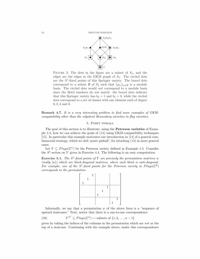
Figure 3. The dots in the figure are a subset of S4, and theedges are the edges in the GKM graph of S4. The circled dotsare the S1-fixed points of this Springer variety. The boxed dotscorrespond to a subset B of S4 such that {pw}w∈B is a modulebasis. The circled dots would not correspond to a module basissince the Betti numbers do not match: the boxed dots indicatethat this Springer variety has b0 = 1 and b2 = 3, while the circleddots correspond to a set of classes with one element each of degree0, 2, 4 and 6.
Remark 4.7. It is a very interesting problem to find more examples of GKM-compatability other than the nilpotent Hessenberg varieties in flag varieties.
5. Poset pinball
The goal of this section is to illustrate, using the Peterson varieties of Exam-ple 4.3, how we can achieve the goals of (12) using GKM-compatibility techniques[15]. In particular this example motivates our introduction in [14] of a general com-binatorial strategy, which we dub ‘poset pinball’, for attacking (12) in more generalcases.
Let Y ⊆ F`ags(Cn) be the Peterson variety defined in Example 4.3. Considerthe S1-action on Y given in Exercise 4.4. The following is an easy computation.
Exercise 5.1. The S1-fixed points of Y are precisely the permutation matrices w(really [w]) which are block-diagonal matrices, where each block is anti-diagonal.For example, one of the S1-fixed points for the Peterson variety in F`ags(C8)corresponds to the permutation
11
11
11
11
Informally, we say that a permutation w of the above form is a “sequence ofupward staircases.” Next, notice that there is a one-to-one correspondence
(16) Y S1 ⊆ F`ags(Cn) ↔ subsets of {1, 2, . . . , n− 1}given by taking the indices of the columns in the permutation which are not at thetop of a staircase. Continuing with the example above, under this correspondence
EQUIVARIANT SCHUBERT CALCULUS, GKM THEORY AND POSET PINBALL 25
we would identify
11
11
11
11
↔ {1, 2, 4, 5, 7}.
(Here the indices “not at the top of a staircase” are boxed for the purpose ofillustration.) We set the following notation for the correspondence given in (16):
wA ↔ A.
Recalling (15), we wish to choose a vA ∈ Sn for each wA such that {pvA}A⊆{1,2,3,...,n−1}forms a module basis for H∗
S1(Y ). It turns out that in this case we can explicitlydescribe the appropriate choices of vA. Namely, define
vA :=∏
i∈Asi.
For example, if A = {1, 2, 4, 5, 7} then vA = s1s2s4s5s7.We quote the following from [15].
Theorem 5.2. (1) vA ≤ wA for all A.(2) vA ≤ wB if and only if wA ≤ wB.(3) Degrees of {pvA} are compatible with (known) Betti numbers of Y .
• deg pvA = 2l(vA) = 2 ·#A.
• #{pvA | deg pvA = 2k} =(
n− 1k
).
• From [22]: b2k(Y ) =(
n− 1k
), and bodd = 0. (Note that this matches the
preceding point exactly.)
Proof. We sketch proofs of the first two facts. For (1), the maximal inversion(k k − 1 k − 2 · · · 2 1
)
in Sk has reduced word decomposition
s1(s2s1)(s3s2s1) · · · (sk−1sk−2 · · · s2s1),
which implies that pvA(wA) 6= 0. For (2), observe
vA ≤ wB ⇔ A ⊆ B ⇔ wA ≤ wB.
¤
Theorem 5.2 implies that {pvA} is a module basis of H∗S1(Y ), thus partially
achieving (12). In the case of Peterson varieties, we can also do more. The firstobservation is the following.
Theorem 5.3 ([14]). Let pi := pv{i} . The elements {pi}n−1i=1 generate H∗
S1(Y ) as aring.
26 MEGUMI HARADA
The above theorem implies that, in order to compute the ring structure ofH∗
S1(Y ), it suffices to compute products of the form pi · pvA . This is achievedby the S1-equivariant Chevalley-Monk formula for Peterson varieties [15].More specifically, we have
(17) pi · pA = cAi,A · pA +∑
A(B and |B|=|A|+1
cBi,A · pB
for any i and A, where the structure constants are as follows. For any set C ⊆{1, 2, . . . , n− 1} and any ` ∈ C, we denote by TC(`) and HC(`) the unique integerssuch that TC(`) ≤ ` ≤ HC(`), the consecutive sequence {TC(`), TC(`)+1, . . . ,HC(`)−1,HC(`)} is a subset of C, and such that TC(`)− 1 6∈ C,HC(`)+1 6∈ C. We have first
• cAi,A = 0 if i 6∈ A,• cAi,A = (HA(i)− i + 1)(i− TA(i) + 1)t if i ∈ A,
where the variable t is the cohomology-degree-2 generator of H∗S1(pt) ∼= C[t]. Ad-
ditionally, for a subset B ⊆ {1, 2, . . . , n− 1} which is a disjoint union B = A∪ {k},we have
• cBi,A = 0 if i 6∈ {TB(k), TB(k) + 1, . . . ,HB(k)− 1,HB(k)},• if k ≤ i ≤ HB(k), then
cBi,A = (HB(k)− i + 1) ·( HB(k)− TB(k) + 1
k − TB(k)
)
• if TB(k) ≤ i ≤ k − 1, then
cBi,A = (i− TB(k) + 1) ·(HB(k)− TB(k) + 1
k − TB(k) + 1
).
From the above description, it is clear that these Monk formulae for the structureconstants evidently has many of the properties deemed to be desirable in (12):it is explicit, easily computed, and both manifestly positive and manifestlyintegral. Moreover, in follow-up work [1], we also prove a Giambelli formula,which gives a concrete and combinatorial formula expressing an arbitrary modulegenerator pvA in terms of the ring generators pi.
The results for the case of Peterson varieties raises the following tantalizingquestion:
Question 5.4. Can we find analogues of vA for more general Hessenberg varieties?Can we also prove general combinatorial formulae for structure constants using thecorresponding module bases?
The game of poset pinball, briefly introduced next, is a combinatorial approachto answering this question. For more details see [14, Section 3]. Let (J , <) be afinite partially ordered set (e.g., Sn with the Bruhat order). Identify J with itsHasse diagram, which is a directed acyclic graph, with an edge a 7→ b when a coversb in the partial order (i.e., a > b and there does not exist a c with a > c > b). Wesay that J is the board. The vertices are slots. At most one pinball can occupya given slot at any time. The directed edges are called slides.
Fix a subset I ⊂ J , called the initial subset. (The motivating example ifI = Hess(X, h)S1
and J = Sn). At the start of the game, place a pinball ateach slot corresponding to an element of I. During the game, we occasionally placewalls across some slides, which prevents a ball from rolling down that slide. (When
EQUIVARIANT SCHUBERT CALCULUS, GKM THEORY AND POSET PINBALL 27
a ball at slot a is released, it may roll down a slide from a to a slot b, if a 7→ b isan edge).
Fix a total order ≺ on I subordinate to the partial order induced from J . Weroll pinballs in order with respect to ≺. By this we mean:
(F)Given a pinball at slot a, consider the set:{b ∈ J : a 7→ b and there is no wall across a 7→ b}.
If (F) is non-empty, pick an element b and roll to it. (Note this process is non-deterministic – just like real arcade-game pinball!) Replace a by b, and repeat untilthe relevant set (F) is empty; i.e., it can roll no further (so all lower slots arealready occupied by previously rolled pinballs). Call the result of this procedure(i.e., the name the slot where the pinball ends) the rolldown of a and we denotethis process by a 7→ roll(a).
The motivation behind this game is the following.
Fact 5.5. The vA associated to wA in the Peterson case is the outcome of a gameof poset pinball.
The real point, however, is that poset pinball can be played for other cases ofHessenberg varieties, not just for Peterson varieties, as the next example shows.
Example 5.6. We revisit in this context the nilpotent Springer variety in F`ags(C4)corresponding to the Young diagram (3, 1), already discussed in Figure 3. One pos-sible outcome of a basic pinball game is as follows:
t
t
t
t
t t t
t t t
@@
@
¡¡
¡
¡¡
¡
@@
@
¡¡
¡
¡¡
¡
@@
@
@@
@
i
i
i
ie
s3s2s1
s3s2s3s1s2s1
s3s2s1
where the circled permutations correspond to the S1-fixed points, and the squareddots are their rolldowns. However, as noted above, basic pinball is not deterministic.Thus another possible outcome is:
t
t
t
t
t t t
t t t
@@
@
¡¡
¡
¡¡
¡
@@
@
¡¡
¡
¡¡
¡
@@
@
@@
@
i
i
i
ie
s3s2s1
s3s2s3s1s2s1
s3s2s1
It is the outcome of the first game in Example 5.6 that actually gives rise to amodule basis of the S1-equivariant cohomology of this Springer variety (as alreadynoted in the discussion of Figure 3). It turns out that one can place additional
28 MEGUMI HARADA
restrictions on the game of poset pinball in order to ‘rule out’ the possibility of thesecond outcome, which is not desirable for several reasons, including that the Bettinumbers do not match (cf. discussion of Figure 3). We refer the reader to [14,Section 3] for more details.
Finally, as discussed above, we can also construct geometric representations onS1-equivariant cohomology rings using our techniques. Subregular Springer va-rieties are those Springer varieties corresponding to the Young diagram (n− 1, 1)for some n ∈ Z>0. For fixed n, let Sn−1,1 denote the associated subregular Springervariety. Using module bases obtained via poset pinball, we can prove the followingresult.
Theorem 5.7 ([14]). The images of {σl, σs1 , . . . , σsn−1} under the natural mapH∗
T (F`ags(Cn)) → H∗S1(Sn−1,1) form a module basis for H∗
S1(Sn−1,1).
Remark 5.8. By exploiting this, we can build an S1-equivariant lift of the classicalSpringer action on H∗(Sn−1,1) to H∗
S1(Sn−1,1). We refer the reader to [14, Section6.3] for details.
We close these lectures with a brief description of the results in [2, 7]. The manu-script [2] deals with regular nilpotent Hessenberg varieties with h = (3, 3, 4, 5, . . . , n−1, n). These should be thought of as regular nilpotent Hessenberg varieties whichare very close to the Peterson variety. In the analysis of the Peterson case, it wascrucial that we had an explicit formula for the rolldown vA corresponding to eachfixed point wA. In [2] we further develop the poset pinball theory by proposing, forthe case of regular nilpotent Hessenberg varieties, an analogous explicit algorithmfor producing reduced word decompositions of the rolldowns roll(w) for the fixedpoints w ∈ Hess(X, h)S1
. (We dub this the dimension pair algorithm, since it isbased on the notion of dimension pairs introduced in [19].) While the algorithm isnot as easily stated as for the Peterson case, it nevertheless allows us to explicitlyanalyze the case when the Hessenberg function is of the form h = (3, 3, 4, 5, ...), andin particular to prove using hands-on combinatorics that the result does indeedyield a module basis of S1-equivariant cohomology.
The manuscript [7], on the other hand, deals with the Springer varieties Sn−2,2
corresponding to the Young diagram (n − 2, 2) for some n ≥ 4. These should bethought of as Springer varieties which are very close to the subregular Springervarieties Sn−1,1 analyzed in Theorem 5.7 above. Using a version of the dimensionpair algorithm introduced in [2], Dewitt and I use the Billey formula and someexplicit combinatorial computations to prove that, also in the case of Sn−2,2, theresult of poset pinball obtained by the dimension pair algorithm produces a modulebasis for S1-equivariant cohomology.
As is evident from the descriptions above, research in this area is just beginning.We refer the reader to the manuscripts [15, 14, 2, 7] for more detailed lists of openquestions and possible future work, but roughly speaking the questions can besummarized as follows:
• Is there a wider class of examples of Hessenberg varieties Hess(X,h) whereone can produce a provable and explicit algorithm for pinball rolldownswhich correspond to a module basis of H∗
S1(Hess(X, h))?• Can we derive explicit, combinatorial formulae for structure constants with
respect to well-chosen such module bases?
EQUIVARIANT SCHUBERT CALCULUS, GKM THEORY AND POSET PINBALL 29
• Can we use these module bases to construct geometric representations onequivariant cohomology rings?
References
[1] D. Bayegan and M. Harada. A Giambelli formula for the S1-equivariant cohomology of typeA Peterson varieties, 2010, arXiv:1012.4053. To be published in Involve.
[2] D. Bayegan and M. Harada. Poset pinball and type A regular nilpotent Hessenberg varieties,2010, arXiv:1012.4054. To be published in ISRN Geometry.
[3] S. Billey. Kostant polynomials and the cohomology ring of G/B. Duke Math. J., 96:205–224,1999.
[4] M. Brion and J. B. Carrell. The equivariant cohomology ring of regular varieties. MichiganMath. J., 52(1):189–203, 2004.
[5] J. B. Carrell and K. Kaveh. On the equivariant cohomology of subvarieties of a B-regularvariety. Transform. Groups, 13(3-4):495–505, 2008.
[6] F. De Mari, C. Procesi, and M. A. Shayman. Hessenberg varieties. Trans. Amer. Math. Soc.,332(2):529–534, 1992.
[7] B. Dewitt and M. Harada. Poset pinball, highest forms, and (n − 2, 2) Springer varieties,2010, arXiv:1012.5265.
[8] J. Fulman. Descent identities, Hessenberg varieties, and the Weil conjectures. J. Combin.Theory Ser. A, 87(2):390–397, 1999.
[9] W. Fulton. Young tableaux, volume 35 of London Mathematical Society Student Texts. Cam-bridge University Press, Cambridge, 1997. With applications to representation theory andgeometry.
[10] F. Y. C. Fung. On the topology of components of some Springer fibers and their relation toKazhdan-Lusztig theory. Adv. Math., 178(2):244–276, 2003.
[11] M. Goresky, R. Kottwitz, and R. MacPherson. Equivariant cohomology, Koszul duality, andthe localization theorem. Invent. Math., 131:25–83, 1998.
[12] V. Guillemin, T. Holm, and C. Zara. A GKM description of the equivariant cohomology ringof a homogeneous space. J. Algebraic Combin., 23:2141, 2006.
[13] V. W. Guillemin and S. Sternberg. Supersymmetry and equivariant de Rham theory. Math-ematics Past and Present. Springer-Verlag, Berlin, 1999.
[14] M. Harada and J. Tymoczko. Poset pinball, GKM-compatible subspaces, and Hessenbergvarieties, arXiv:1007.2750.
[15] M. Harada and J. Tymoczko. A positive Monk formula in the S1-equivariant cohomology oftype A Peterson varieties. Proc. London Math. Soc., 2011. doi: 10.1112/plms/pdq038.
[16] S. L. Kleiman and D. Laksov. Schubert calculus. Amer. Math. Monthly, 79:1061–1082, 1972.[17] A. Knutson. A Schubert calculus recurrence from the noncomplex W -action on G/B, June
2003, math.CO/0306304.[18] B. Kostant. Flag manifold quantum cohomology, the Toda lattice, and the representation
with highest weight ρ. Selecta Math. (N.S.), 2(1):43–91, 1996.[19] A. Mbirika. A Hessenberg generalization of the Garsia-Procesi basis for the cohomology ring
of Springer varieties. Electronic Journal of Combinatorics, 17 (electronic), 2010.[20] K. Rietsch. Totally positive Toeplitz matrices and quantum cohomology of partial flag vari-
eties. J. Amer. Math. Soc., 16(2):363–392 (electronic), 2003.[21] N. Shimomura. The fixed point subvarieties of unipotent transformations on the flag varieties.
J. Math. Soc. Japan, 37(3):537–556, 1985.[22] E. Sommers and J. Tymoczko. Exponents for B-stable ideals. Trans. Amer. Math. Soc.,
358(8):3493–3509 (electronic), 2006.[23] N. Spaltenstein. The fixed point set of a unipotent transformation on the flag manifold.
Nederl. Akad. Wetensch. Proc. Ser. A 79=Indag. Math., 38(5):452–456, 1976.[24] J. S. Tymoczko. An introduction to equivariant cohomology and homology, following Goresky,
Kottwitz, and MacPherson, arXiv:math.AG/0601681.[25] J. S. Tymoczko. Linear conditions imposed on flag varieties. Amer. J. Math., 128(6):1587–
1604, 2006.[26] J. S. Tymoczko. Paving Hessenberg varieties by affines. Selecta Math. (N.S.), 13(2):353–367,