Lectures on Higher Structures in M-theory

Christian Samann

Maxwell Institute for Mathematical Sciences

Department of Mathematics, Heriot-Watt University

Colin Maclaurin Building, Riccarton, Edinburgh EH14 4AS, U.K.

Email: c.saemann@hw.ac.uk

Abstract

These are notes for four lectures on higher structures in M-theory as presented

at workshops at the Erwin-Schrodinger Institute and Tohoku University. The

first lecture gives an overview of systems of multiple M5-branes. In the second

lecture, the relevant mathematical structures are introduced to describe higher

gauge theory both locally and globally. A construction of non-abelian super-

conformal gauge theories in six dimensions using twistor spaces is discussed in

the third lecture. The last lecture deals with the problem of higher quantization

and its relation to loop space. An appendix summarizes the relation between

3-Lie algebras and Lie 2-algebras.

Version April 2, 2016

Contents

1 Introduction 2

2 Higher gauge theory arising in M-theory 3

2.1 Motivation: Systems of multiple M5-branes . . . . . . . . . . . . . . . . . . 3

2.2 Obstacles to constructing classical non-abelian (2,0)-theories . . . . . . . . . 4

2.3 Self-dual strings . . . . . . . . . . . . . . . . . . . . . . . . . . . . . . . . . . 6

2.4 Higher Lie algebras . . . . . . . . . . . . . . . . . . . . . . . . . . . . . . . . 7

2.5 Local higher gauge theory . . . . . . . . . . . . . . . . . . . . . . . . . . . . 9

2.6 Further reading . . . . . . . . . . . . . . . . . . . . . . . . . . . . . . . . . . 10

3 Categorification 11

3.1 (Strict) 2-categories . . . . . . . . . . . . . . . . . . . . . . . . . . . . . . . 11

3.2 Strict 2-groups . . . . . . . . . . . . . . . . . . . . . . . . . . . . . . . . . . 12

3.3 Principal bundles as functors . . . . . . . . . . . . . . . . . . . . . . . . . . 13

3.4 Principal 2-bundles . . . . . . . . . . . . . . . . . . . . . . . . . . . . . . . . 14

3.5 Differentiating Lie 2-groups . . . . . . . . . . . . . . . . . . . . . . . . . . . 14

3.6 Summary of the construction . . . . . . . . . . . . . . . . . . . . . . . . . . 15

3.7 Further reading . . . . . . . . . . . . . . . . . . . . . . . . . . . . . . . . . . 16

4 Constructing (2,0)-theories 16

4.1 Twistors . . . . . . . . . . . . . . . . . . . . . . . . . . . . . . . . . . . . . . 16

4.2 Solutions to integrable field equations . . . . . . . . . . . . . . . . . . . . . 18

4.3 Twistor space for self-dual 3-forms . . . . . . . . . . . . . . . . . . . . . . . 19

4.4 Deriving a (2,0)-theory . . . . . . . . . . . . . . . . . . . . . . . . . . . . . . 19

4.5 Further reading . . . . . . . . . . . . . . . . . . . . . . . . . . . . . . . . . . 20

5 Higher quantization 20

5.1 Motivation: Fuzzy funnel in M-theory . . . . . . . . . . . . . . . . . . . . . 20

5.2 Observables on 2-plectic manifolds . . . . . . . . . . . . . . . . . . . . . . . 21

5.3 Quantization of multisymplectic manifolds . . . . . . . . . . . . . . . . . . . 22

5.4 Transgression to loop space . . . . . . . . . . . . . . . . . . . . . . . . . . . 23

5.5 Towards a quantization of loop space . . . . . . . . . . . . . . . . . . . . . . 24

Appendix 26

A Higher Lie algebras and 3-Lie algebras . . . . . . . . . . . . . . . . . . . . . 26

1

1. Introduction

The purpose of these lectures is to provide a motivation for studying higher structures

within M-theory and to give some feeling for the mathematical language underlying these

structures. In particular, we will review a very general approach to principal bundles

with connections, which allows for a very large class of generalizations, including higher

gauged sigma models on representable higher differential stacks. This includes higher gauge

theories on ordinary manifolds, orbifolds and categorified spaces. This approach yields the

global geometry bundle structure, the appropriate definition of curvatures and the finite

gauge transformations.

My personal interest in such constructions stems from the problem of finding a classical

description of the superconformal field theory in six dimensions with non-abelian gauge

structure. This theory is usually referred to as the (2, 0)-theory, as it has N = (2, 0)

supersymmetry. It is well known that the free or abelian (2, 0)-theory contains a 2-form

curvature on a U(1)-gerbe. Therefore it is natural to expect that a non-abelian theory is

based on non-abelian gerbes, which are categorifications of principal 2-bundles. In order

to look for a non-abelian (2, 0)-theory, one should first understand the geometric setup for

the gauge sector.

Once this is done, there is a very natural and direct route to constructing corresponding

(2, 0)-theories. Recall that solutions to the N = 4 Yang-Mills equations in four dimensions

can be described by certain holomorphic principal bundles over a suitable twistor space.

Similarly, a twistor space for self-dual 3-form curvatures in six dimensions is known. It is

easy to extend this picture supersymmetrically, and we can consider more general holomor-

phic higher principal bundle over the resulting twistor space. In the case of holomorphic

principal 2-bundles, this yields precisely the field content of the (2, 0)-theory, together with

superconformal field equations.

In a second part, I discuss higher quantization, a topic which is closely related to the

definition of the (2, 0)-theory. Essentially, one would expect that the higher endomorphisms

on the resulting higher Hilbert spaces form the higher gauge algebras for the (2, 0)-theory,

as well as for generalized M2-brane models.

Since I had only four hours available for the above material, the discussion is necessarily

very concise. I tried to focus on giving impressions of the right point of view1 of various

mathematical objects and how to work with these. The time constraint meant that some

of the discussion had to remain mathematically superficial or even slightly sloppy. For

example, I always avoided talking about internalization, which underlies the transition

from n-groups to Lie n-groups.

I have resisted the temptation of adding material which I did not have time to discuss

in the lecture. I took, however, the liberty of adding footnotes, literature references and re-

marks, providing additional connections between the discussed objects. Also, an appendix

1Sometimes this is also called the n-categorical point of view or n-POV. This n-POV is the one unifying

mathematical objects and their categorification (as well as physics, philosophy, you name it). This point of

view is certainly not neutral, and for that reason there are “right” and “wrong” definitions.

2

addresses the frequently arising question how the 3-Lie algebras of M2-brane models are

related to the categorified Lie algebras used in our constructions.

These notes are not as polished as my journal publications, and I’d be very grateful

for any feedback, comments, corrections etc. leading to improvements. Just send them in

an email to c.saemann@hw.ac.uk and I’ll incorporate them in future versions. The latest

version of these notes can always be found on my homepage, www.christiansaemann.de

Acknowledgements

I would like to thank the organizers of the workshops “Higher Structures in String Theory

and Quantum Field Theory” at the Erwin Schrodinger International Institute for Mathe-

matical Physics, Vienna, as well as “Higher Structures in String Theory and M-Theory” at

Tohoku University, Sendai, during which these lectures were presented. Many thanks also

to Patricia Ritter and Lennart Schmidt for helpful comments on a first version of these

notes.

2. Higher gauge theory arising in M-theory

In this section, we present our motivation for developing higher gauge theory. We intro-

duce higher Lie algebras and give a glimpse of higher gauge theory by presenting its local

description.

2.1. Motivation: Systems of multiple M5-branes

In string theory, interesting vacua are described in terms of D-brane configurations in cer-

tain background geometries with fluxes. The D-branes interact through strings stretched

between them. The endpoints of these strings induce a U(1)-gauge field on the D-branes’

worldvolumes and if we decouple massive modes and gravity, we obtain an effective dy-

namical description in terms of gauge theory. For a very helpful review of the arising gauge

theories, see [1].

When multiple D-branes come together, the abelian gauge symmetry is generally en-

hanced to a non-abelian one. In the simplest case of a flat stack of n D-branes, the gauge

group U(1)× . . .×U(1) is enhanced to U(n). Non-abelian gauge theories are certainly much

richer than abelian ones, as they exhibit new features as e.g. confinement. But even with-

out matter coupling, we have instantons in four dimensions and non-singular monopoles

on R3, which do not exist in the abelian case.

A particularly interesting example of such a gauge theory is N = 4 super Yang-Mills

theory on Minkowski space R1,3. This theory arises from a stack of flat D3-branes and

correspondingly has 16 real supersymmetries. Its classical superconformal symmetry is

preserved at quantum level, and it is the conformal field theory in the famous holographic

correspondence on AdS5 × S5.

In M-theory, the situation is similar. We can describe interesting vacua as M-brane

configurations in background geometries with fluxes. Contrary to the rich spectrum of

3

D-branes in type II superstring theory, there are (essentially) only M2- and M5-branes in

M-theory. M5-branes interact through M2-branes ending on them and their boundaries

form tensionless “self-dual” strings. Because they are essentially massless, supergravity

decouples from the dynamics of these strings. Effectively they should be described by a six

dimensional N = (2, 0)-supersymmetric conformal field theory. This theory, which we well

call (2, 0)-theory for short in the following, is in some sense the six dimensional analogue of

N = 4 super Yang-Mills theory in four dimensions. The field content of the (2, 0)-theory

consists of the N = (2, 0)-tensor multiplet in six dimensions. Its bosonic sector is given

by a self-dual 3-form curvature H := dB = ∗H of a 2-form potential B and five scalars,

which are the Goldstone modes of the breaking of the symmetries from R1,10 to R1,5×R5

by the presences of the M5-brane. For a review of M-brane dynamics, see [2].

Mathematically, the 2-form potential B is the curving of an abelian gerbe or an abelian

principal 2-bundle and dynamical theories of such higher form potentials on higher principal

bundles are known as higher gauge theories. An important problem is now the non-abelian

generalization of these structures, which should underlie an effective description of stacks

of multiple M5-branes. There is huge interest in such a theory in both the physics and

the mathematics communities, as it would boost our understanding of M-theory and shed

light on many issues, as e.g. AGT relations, the Geometric Langlands duality and M-theory

in general. The large part of these lectures will deal with approaches towards defining a

classical description of the (2,0)-theory.

2.2. Obstacles to constructing classical non-abelian (2,0)-theories

A point particle charged under a gauge group G is described by its position and a point of

in a representation space of G. More precisely, it is described by a point in a corresponding

associated vector bundles to a principal G-bundle. Recall that given a cover tiUi → M

of a manifold M in terms of local patches Ui, such a principal bundle is given by a set of

transition functions gij : Uij → G satisfying

gijgjk = gik (2.1)

on all non-empty triple intersections Ui ∩ Uj ∩ Uk. Mathematically, these functions form

a (non-abelian) Cech 1-cocycle. Cech 1-cocycles are extended to Deligne 1-cocycles by

adding a set of Lie(G)-valued connection 1-forms Ai ∈ Ω(Ui) ⊗ Lie(G), which are glued

together by the relation

Aj = g−1ij Aigij + g−1

ij dgij (2.2)

on non-empty double intersections Ui ∩ Uj . Gauge transformations are parameterized by

functions γi : Ui → G, which form Deligne coboundaries between Deligne 1-cocycles (g,A)

and (g, A) according to

γigij = gijγj and Ai = γ−1i Aiγi + γ−1

i dγi . (2.3)

Deligne 1-cocycles modulo Deligne 1-coboundaries yield Deligne cohomology classes which

describe principal G-bundles with connection modulo gauge transformations.

4

The potential one-forms Ai give rise to a map from a path γ in M to a group element

g(γ) = P exp

∫γA , (2.4)

where P stands for path ordering. This map encodes the parallel transport of G-charged

particles along the path γ.

We can regard the curve γ as the boundary of an open string on a D-brane, i.e. an

endpoint of a string moving through time. In M-theory, one would consider analogously

the boundary of an M2-brane ending on an M5-brane, which gives rise to the previously

mentioned “self-dual strings.” To describe a parallel transport of self-dual strings along a

surface σ, we are naturally led to introducing a 2-form B. In the abelian case, we can then

write

g(σ) = exp

∫σB , (2.5)

but since there is no reparametrization invariant notion of surface ordering, this equation

does not extend to the non-abelian case. More explicitly, when considering a parallel

transport of a self-dual string subdivided into two pieces as follows

oo ]]g1

g′1

oo ]]g2

g′2

(2.6a)

we need that

(g′1g′2)(g1g2) = (g′1g1)(g′2g2) (2.6b)

since the order in which we parallel transport the top string to the bottom one should

be irrelevant. By an argument going back to Eckmann and Hilton [3], this forces G to

be abelian. It is essentially this argument that underlies many of the no-go-theorems in

the physics literature which forbid the existence of a non-abelian parallel transport along

surfaces.

Fortunately, the assumptions here are a little too naive. Note that the map from curves

γ to group elements is in fact part of a functor, and it is very natural to assume that a

corresponding map from surfaces should be a 2-functor. Indeed, the objects appearing in

(2.6) suggest that we have objects (•), 1-morphisms (←−) and 2-morphisms (⇐=). It is

also clear from the diagram that the 1-morphisms can be composed horizontally, which

induces a horizontal composition of the 2-morphisms. Both combine into a functor, which

we will denote by ⊗. Moreover, there is a vertical composition of 2-morphisms. This is

the structure appearing in the definition of a 2-category, and a direct consequence of the

axioms for 2-categories is the appropriate form of equation (2.6b),

(g′1 ⊗ g′2) (g1 ⊗ g2) = (g′1 g1)⊗ (g′2 g2) , (2.7)

which is known as the interchange law.

Having removed the mathematical obstacles to constructing a classical (2, 0)-theory, let

us consider some arguments from string theory. Since the (2, 0)-theory is conformal we

5

know that there are no dimensionful parameters in the theory. Contrary to N = 4 super

Yang-Mills theory, however, string theory suggests that the relevant superconformal fixed

points in parameter space are isolated and therefore there are no continuous parameters

either. This suggests that there is no Lagrangian description.

Note, however, that the same arguments were true for M2-branes, and successful M2-

brane models have been constructed [4, 5, 6]. While there are no continuous parameters in

these models, there is a discrete one, k ∈ Z, arising from the background geometry R8/Zkin which the M2-branes are placed. We can expect that the same happens in the case of

M5-branes.

Even if one is more skeptical about the existence of a classical description of the (2, 0)-

theory, one might still hope for a classical description of the BPS subsector of the theory.

Finally, if even this should turn out to be false, one may learn interesting facts about the

(2, 0)-theory by studying quantum features of the non-abelian higher gauge theories that

we will develop in the following.

2.3. Self-dual strings

Let us now try to get some more intuition about the degrees of freedom underlying the

(2, 0)-theory. Consider the description of monopoles in type IIA superstring theory as

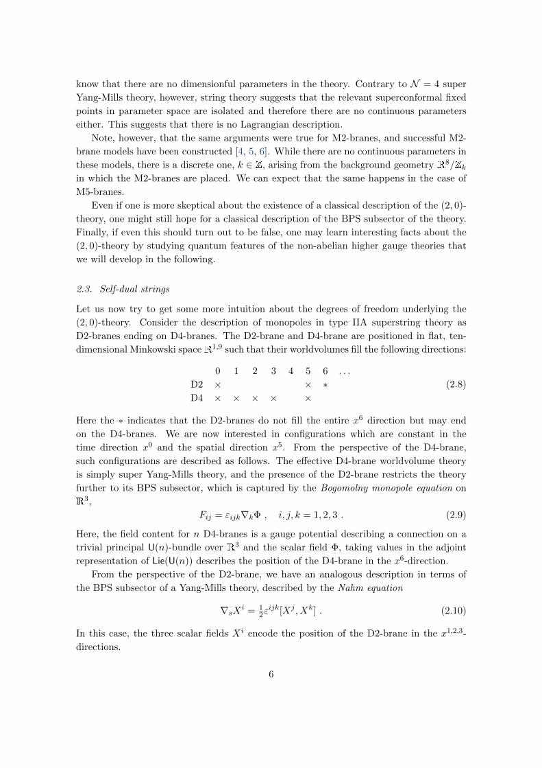
D2-branes ending on D4-branes. The D2-brane and D4-brane are positioned in flat, ten-

dimensional Minkowski spaceR1,9 such that their worldvolumes fill the following directions:

0 1 2 3 4 5 6 . . .

D2 × × ∗D4 × × × × ×

(2.8)

Here the ∗ indicates that the D2-branes do not fill the entire x6 direction but may end

on the D4-branes. We are now interested in configurations which are constant in the

time direction x0 and the spatial direction x5. From the perspective of the D4-brane,

such configurations are described as follows. The effective D4-brane worldvolume theory

is simply super Yang-Mills theory, and the presence of the D2-brane restricts the theory

further to its BPS subsector, which is captured by the Bogomolny monopole equation on

R3,

Fij = εijk∇kΦ , i, j, k = 1, 2, 3 . (2.9)

Here, the field content for n D4-branes is a gauge potential describing a connection on a

trivial principal U(n)-bundle over R3 and the scalar field Φ, taking values in the adjoint

representation of Lie(U(n)) describes the position of the D4-brane in the x6-direction.

From the perspective of the D2-brane, we have an analogous description in terms of

the BPS subsector of a Yang-Mills theory, described by the Nahm equation

∇sXi = 12εijk[Xj , Xk] . (2.10)

In this case, the three scalar fields Xi encode the position of the D2-brane in the x1,2,3-

directions.

6

Interestingly, there is a duality between these two descriptions known as the Nahm

transform. This includes the ADHMN-construction, which maps solutions to the Nahm

equation to solutions to the Bogomolny monopole equation. This can be used to describe

and study the moduli space of monopoles in a very efficient manner.

We can now lift the configuration (2.8) up to M-theory, using the x4-directions as the

M-theory direction:M 0 1 2 3 4 5 6

M2 × × ∗M5 × × × × × ×

(2.11)

In the abelian case of a single M2-brane, this configuration is described by the self-dual

string equation [7]

Hµνκ := ∂[µBνκ] = εµνκλ∂λΦ , µ, ν, κ, λ = 1, . . . , 4 , (2.12)

where Bµν is a potential 2-form on a trivial U(1)-gerbe over R4. As a description from the

perspective of the M5-brane, Basu and Harvey [8] suggested the following equation:

d

dsXµ = 1

3!εµνκλ[Xν , Xκ, Xλ] , Xµ ∈ A , (2.13)

where [−,−,−] denotes some totally antisymmetric ternary bracket on some internal vector

space; see appendix A for details. This equation has led to the development of the M2-brane

models [4, 5, 6], and we also expect that it can teach us more about M5-branes.

There are now two important problems to address. First, we should extend the self-dual

string equation to the non-abelian setting. Second, we should try to establish a duality

between the self-dual string equation and the Basu-Harvey equation analogous to the Nahm

transform. The second problem would have very interesting mathematical implications. We

will address the first problem in the following, and our discussion provides in principle a

starting point for the second one.

2.4. Higher Lie algebras

An N-manifold M is an N-graded manifold. That is, its algebra of functions or, more

precisely, its structure sheaf is generated by elements of degree 0, 1, 2, . . .. These generators

can be regarded as coordinates onM, and thereforeM consists of a body M0 together with

linear spaces fibered over the body:

M = (M0 ←−M1 ←−M2 ←− . . .) . (2.14)

An NQ-manifold is an N-graded manifold together with a vector field Q of degree 1, which

satisfies Q2 = 0. We call such a vector field a homological vector field. NQ-manifolds

are used in physics for BRST quantization as well as in closed string field theory, while

mathematicians know them as differential graded algebras used, e.g., in the Chevalley-

Eilenberg description of Lie algebras.

Let us explain the latter in more detail. Consider an N-manifold concentrated in degree

1. That is M consists exclusively of a vector space g and all vectors have degree 1. We

7

also write M = g[1]. Let us introduce coordinates (ξα) on g[1] of degree 1. A homological

vector field on M is then necessarily of the form

Q = −12ξαξβfγαβ

∂

∂ξγ, (2.15)

where the fγαβ are some constants and the prefactor of −12 is inserted for convenience. The

identity Q2 = 0 is readily seen to be equivalent to the Jacobi identity for a Lie bracket

with structure constants fγαβ.

We can now readily define strong homotopy Lie algebras or L∞-algebras and L∞-

algebroids. An n-term L∞-algebroid is an NQ-manifold concentrated in degrees 0, . . . , n.

An n-term L∞-algebra is an NQ-manifold concentrated in degrees 1, . . . , n. In particular,

we saw above the example of a general 1-term L∞-algebra and this is simply a Lie algebra.

In general, n-term L∞-algebras are categorically equivalent to semistrict Lie n-algebras.

We will be slightly sloppy and use the term n-term L∞-algebra and Lie n-algebra inter-

changeably, because the former are most convenient for describing higher gauge algebras

in higher gauge theories.

We are mostly interested in Lie 2-algebras, and therefore let us look at 2-term L∞-

algebras in more detail. Here, we have the NQ-manifold

M = (∗ ← g[1]← h[2]← ∗ ← . . .) (2.16)

and we use coordinates ξα and χκ of degree 1 and 2 on g[1] and h[2], respectively. The

homological vector field is necessarily of the form

Q = ±mακχ

κ ∂

∂ξα± 1

2fγαβξ

αξβ∂

∂ξγ±mλ

ακξαχκ

∂

∂χλ± 1

3!mκαβγξ

αξβξγ∂

∂χκ, (2.17)

and we shall address the correct signs later. On the shifted vector space L = M[−1] =

g[0]⊕ h[1], with graded basis (τα, σκ), Q induces higher products µk of degree k − 2:

µ1(σκ) := mακτα ,

µ2(τα, τβ) := fγαβτγ , µ2(τα, σκ) := mλακσλ ,

µ3(τα, τβ, τγ) := mκαβγσκ .

(2.18)

Lie 2-algebras with trivial µ3 are called strict Lie 2-algebras.

The relation Q2 amounts to the homotopy Jacobi identity,∑i+j=n

∑σ

χ(σ; `1, . . . , `n)(−1)i·jµj+1(µi(`σ(1), · · · , `σ(i)), `σ(i+1), · · · , `σ(i+j)) = 0 (2.19)

for all `i ∈ L, where the sum runs over all unshuffles, i.e. permutations σ with σ(1) <

. . . < σ(i) and σ(i+ 1) < . . . < σ(i+ j). The graded Koszul sign χ(σ; `1, · · · , `n) is defined

implicitly by the equation

`1 ∧ · · · ∧ `n = χ(σ; `1, · · · , `n) `σ(1) ∧ · · · ∧ `σ(n) . (2.20)

8

That is, write the permutation σ as a sequence of swaps of neighboring objects and count

the number s of such swaps involving at least one object of even degree. The Koszul sign

is then (−1)s.

Exercise: Fix the signs in (2.17) such that (2.18) is compatible with (2.19).

Note that equivalently, we can invert the grading to a non-positive one, resulting in an

L∞-algebra L = h[−1]⊕ g[0], in which the brackets µk carry degree 2− k.

2.5. Local higher gauge theory

As a first step towards higher gauge theory, let us develop a local description of the neces-

sary kinematical data. This involves the definition of higher gauge potential forms, curva-

ture forms as well as the notion of infinitesimal gauge transformations over a contractible

manifold M for a given Lie 2-algebra L.

Recall that there is a natural equation on an L∞-algebra L, the so-called homotopy

Maurer–Cartan equation, ∑i

(−1)k(k+1)/2

k!µk(φ, . . . , φ) = 0 , (2.21)

An element φ ∈ L satisfying this equation is called a Maurer–Cartan element. Note that

these equations are invariant under the infinitesimal gauge transformations

φ→ φ+ δφ with δφ =∑k

(−1)k(k−1)/2

(k − 1)!µk(γ, φ, . . . , φ) , (2.22)

where γ is a degree 0 element of L.

In order to define curvatures, we have to combine the L∞-algebra L with the differential

graded algebra given by the de Rham complex on M , (Ω•(M),d). This is done by taking

the tensor product of both algebras, which always carries a natural L∞-algebra structure2.

More precisely, we take the tensor product of Ω• with that of L, which has the inverted

grading of L and truncate to elements of positive degree, L≥0 := (Ω•(M)⊗ L)≥0. The total

grading of an element of L≥0 is the de Rham grading plus the grading in L, |α⊗`| = |α|+|`|.Explicitly, the vector subspace of degree p-elements for p ≥ 0 is given by

(L≥0)p = (Ωp(M)⊗ L0)⊕ (Ωp+1(M)⊗ L−1) . (2.23)

For a tuple of elements (α1 ⊗ `1, . . . , αk ⊗ `k) of L≥0, the higher products µk read as

µk(α1 ⊗ `1, . . . , αk ⊗ `k) =

(dα1)⊗ `1 + (−1)deg(α1)α1 ⊗ µ1(`1) for k = 1 ,

±α1α2 · · ·αk ⊗ µk(`1, . . . , `k) for k > 1 .

(2.24)

2This holds actually for the tensor product of an arbitrary differential N-graded algebra and an L∞-

algebra.

9

Here, the µk are the higher products in L, deg denotes the degrees in Ω•, and the sign ±in the case k > 1 arises from moving graded elements of Ω• past graded elements of L.

We can now consider Maurer–Cartan elements on L≥0 and read off higher curvatures

and infinitesimal gauge transformations. For an element φ = A − B of degree 1, where

A ∈ Ω1(M) ⊗ L0 and B ∈ Ω2(M) ⊗ L−1, the homotopy Maurer–Cartan equations (2.21)

read asF := dA+ 1

2µ2(A,A)− µ1(B) = 0 ,

H := dB + µ2(A,B)− 13!µ3(A,A,A) = 0 .

(2.25)

Correspondingly, the infinitesimal gauge transformations parametrized by a degree 0 ele-

ment γ = ω + Λ with ω ∈ Ω0(M)⊗ L0 and Λ ∈ Ω1(M)⊗ L−1 are given by

δA = dω + µ2(A,ω)− µ1(Λ) ,

δB = −dΛ− µ2(A,Λ) + µ2(B,ω) + 12µ3(ω,A,A) .

(2.26)

In this way, we can construct the local higher curvatures and infinitesimal gauge transfor-

mations for higher gauge theory on any spacetime carrying a differential graded algebra

and for any gauge L∞-algebra.

Exercise: Derive formulas (2.25) and (2.26).

If one performs a detailed analysis of parallel transport via functors from higher path

groupoids to the delooping of higher gauge groups as done in [9], one finds that reparametri-

zation invariance of the surfaces and higher dimensional volumes involved requires all but

the highest curvature form to vanish.

Being very optimistic, we can now postulate equations of motion for the gauge part of

a theory of multiple M5-branes. The field content consists of a degree 1-element A−B in

L≥0 for some gauge Lie 2-algebra L, which satisfies the equations

H = ∗H and F = dA+ µ2(A,A)− µ1(B) = 0 . (2.27)

Note that the additional degrees of freedom contained in the one-form potential are fully

fixed by the 2-form potential B by the equation F = 0.

2.6. Further reading

The holonomy functor is explained in great detail in [10] and [9]. A detailed discussion of

self-dual strings and the duality can be found e.g. in section 3 of [11]. NQ-manifolds and

their relation to L∞-algebras are reviewed in [12, 13], where also the homotopy Maurer-

Cartan equations and their infinitesimal gauge symmetries are found. See also [14] for

a discussion in the context of string field theory. The construction of local higher gauge

theory as done in the previous section was first given in [15].

10

3. Categorification

Let us now come to the mathematical concepts which will allow us to turn our notion

of local higher gauge theory into a global one. For simplicity, we shall focus on strict 2-

categories, strict 2-groups and strict Lie 2-algebras. A more general picture based on weak

2-categories (which are also known as bicategories) is found in [15].

3.1. (Strict) 2-categories

Formally, a 2-category is a category enriched over Cat. More explicitly, the idea here is

to have objects (points), morphisms (oriented lines) and morphisms between morphisms

(oriented surfaces):

a b

f1

f2

__ α

(3.1)

A strict 2-category C consists of a set3 of objects C0, denoted a, b, c, . . . and for each pair

of objects (a, b) a category C (a, b) of morphisms. This category contains objects, called

1-morphisms f(a, b) and morphisms, called 2-morphisms α(f1, f2). The composition in C (a, b) is known as vertical composition, as the composed 2-morphisms are vertically

composed in diagrams such as (2.6). There is also a functor ⊗ : C (a, b) × C (b, c) →C (a, c), known as horizontal composition. Everything is unital and associative, and we

automatically get the interchange law

(β′ β)⊗ (α′ α) = (β′ ⊗ α′) (β ⊗ α) , (3.2)

cf. (2.7).

Just as the category Set is the “mother of all categories,” the 2-category Cat, consisting

of categories, functors and natural transformations, is the mother of all 2-categories.

To define 2-functors, we note that the ordinary definition is not quite sufficient for our

purposes, and we need to generalize to pseudofunctors. Such a pseudofunctor between two

2-categories C and D is given by

• a function Φ0 : C0 → D0,

• a functor Φab1 : C (a, b)→ D(Φ0(a),Φ0(b)),

• a 2-morphisms Φabc2 : Φab

1 (f)⊗D Φbc1 (g)⇒ Φac

1 (f ⊗C g),

• a 2-morphism Φa2 : idΦ0(a) ⇒ Φaa

1 (ida).

The last two 2-morphisms are responsible for the prefix ‘pseudo.’ We can restrict ourselves

to normalized pseudofunctors, i.e. pseudofunctors with Φa2 the identity. We still have a

3We simplify to small categories.

11

compatibility relation for the 2-cells given by Φabc2 , which arises from the diagram

· · ·

$,(Φab

1 (x) ⊗Φbc1 (y)) ⊗Φcd

1 (z)

Φabc2 ⊗id

19

=

Φad1 ((x⊗ y)⊗ z)

=

Φab1 (x) ⊗ (Φbc

1 (y) ⊗Φcd1 (z))

%-

Φad1 (x⊗ (y ⊗ z))

· · ·

2:

(3.3)

Exercise: Label the arrows and fill in the · · · . From the commutativity of the diagram,

write down the equation satisfied by the Φabc2 . The answer for weak 2-categories, which

reduce for trivial associators and unitors to the strict case, is given in [15].

Analogously, one defines natural 2-transformations, and details can be found e.g. in

[15].

3.2. Strict 2-groups

The first ingredient in the definition of a principal bundle is a structure group, and we

therefore need to find a higher analogue. Note that any group G forms a category with in-

vertible morphisms, BG⇒ ∗, where source and target are trivial, id∗ = 1G and composition

is given by group multiplication.

Correspondingly, we would like to regard a 2-group as a 2-category with a single object

and invertible 1- and 2-morphisms:

BG := (∗⇔ G0 ⇔ G1) , G = (G0 ⇔ G1) = BG (∗, ∗) , (3.4)

and we thus arrive at the notion of a (strict) 2-group.

It has been shown [16] that such a strict 2-group is categorically equivalent to a crossed

module of Lie groups. The latter consists of a pair of Lie groups H,G together with a

homomorphism ∂ : H→ G and an action B: Gn H→ H satisfying

∂(g B h) = g B ∂(h) , ∂(h1) B h2 = h1h2h−11 (3.5)

for all g ∈ G and h, h1,2 ∈ H. To reconstruct the strict 2-group, put

G0 = G , G1 = G n H , s(g, h) = g , t(g, h) = ∂(h)g , id(g) = (g,1) ,

g1 ⊗ g2 = g1g2 , (g1, h1)⊗ (g2, h2) = (g1g2, h1(g1 B h2)) ,

(∂(h1)g, h2) (g, h1) = (g, h2h1) .

(3.6)

Conversely, a crossed module of Lie groups is derived from the strict 2-group G by putting4

H = ker(s) and G = G0.

4look up “Moore complex”

12

Exercise: Complete the inverse map. The solution is found in [16].

3.3. Principal bundles as functors

We now come to the description of principal bundles from the n-POV, which is suitable

for categorification. Recall that the Cech groupoid5 C (Y ) of a surjective submersion π :

Y M has objects Y and morphisms

Y [2] = Y ×M Y := (y1, y2) | π(y1) = π(y2) (3.7)

with obvious structure maps. In the case of an ordinary cover Y = tiUi, the objects are

pairs (x, i) with x ∈ Ui and the morphisms are triples (x, i, j), x ∈ Ui ∩ Uj . We have

s(x, i, j) = (x, j) and t(x, i, j) = (x, i) as well as id(x, i) = (x, i, i), inv(x, i, j) = (x, j, i) and

(x, i, j) (x, j, k) = (x, i, k). This groupoid encodes all necessary information about the

manifold M . Note that the Cech groupoid can trivially be regarded as a 2-groupoid by

adding all identity 2-morphisms. That is, the corresponding 2-category has objects Y and

the categories of morphisms combine to the trivial category Y [2] ⇒ Y [2].

On the other hand, we need to choose a gauge group G, which we regard again as the

groupoid BG := G⇒ ∗.We now define a principal bundle subordinate to the cover Y as a functor C (Y )→ BG.

We have the following diagram

(x, i, j)gij(x) //

G

(x, i) // ∗

(3.8)

where the compatibility with composition contained in the definition of a functor implies

gij(x)gjk(x) = gik(x) on Uijk.

A bundle isomorphism is accordingly given by natural transformations, which are en-

coded in maps γi : Ui → G such that the following diagram commutes:

∗γi(x)

∗γj(x)

gij(x)oo

∗ ∗gij(x)oo

(3.9)

We arrive at the cocycle relation γi(x)gij(x) = gij(x)γj(x) and we recovered the first Cech

cohomology class.

5i.e. a small category with invertible morphisms

13

3.4. Principal 2-bundles

We now have everything at our disposal to define principal 2-bundles: A principal 2-

bundle over a manifold M subordinate to a cover Y M with structure 2-group G is a

normalized pseudofunctor from the Cech 2-groupoid C (Y ) to the 2-groupoid BG . If H∂→ G

is the crossed module of Lie groups corresponding to G , the resulting cocycle is encoded

in functions gij : Uij → G and hijk : Uijk → H satisfying

∂(hijk)gijgjk = gik ,

hiklhijk = hijl(gij B hjkl) .(3.10)

Isomorphisms of principal 2-bundles are natural 2-transformations between the corre-

sponding pseudofunctors.

Exercise: Verify the cocycle condition (3.10) and derive the corresponding coboundary

relations. The answer is found in [15].

Among important examples of principal 2-bundles, we have ordinary, principal G-

bundles for crossed module ∗ ∂→ G, abelian gerbes for crossed module U(1)∂→ ∗ and

twisted principal G-bundles for crossed module U(1)∂→ G. Principal 2-bundles thus indeed

nicely unify non-abelian principal bundles and abelian gerbes.

To add a connective structure to principal 2-bundles, we have to discuss Lie 2-algebras

and how they are obtained, which we shall do next.

3.5. Differentiating Lie 2-groups

An integration of L∞-algebras can be performed [17], but the procedure is very cumber-

some. As always, differentiation is easier than integration, and we therefore start with a

Lie 2-group G . An nPOV on the Lie algebra of a Lie group was suggested by Severa [18].

In this picture, we consider the functor that maps supermanifolds X to descent data for

a principal G -bundle subordinate to the surjective submersion X × R0|1 → X. The Lie

algebra is recovered as the moduli space of such functors.

In particular, descent data for such a principal G -bundle is captured by functions

g : X ×R0|2 → G such that

g(θ0, θ1, x)g(θ1, θ2, x) = g(θ0, θ2, x) , (3.11)

where θ0,1,2 ∈ R0|1 and x ∈ X. This equation immediately implies that

g(θ, θ, x) = 1 and g(θ, 0, x) = (g(0, θ, x))−1 . (3.12)

Therefore,

g(θ0, θ1, x) = g(θ0, 0, x)(g(θ1, 0, x))−1 , (3.13)

14

and fixing the parametrization6

g(θ0, 0, x) = 1+ aθ0 , (3.14)

where a ∈ T1G[1] = g[1], we can compute

g(θ0, θ1) = 1+ a(θ0 − θ1) + 12 [a, a]θ0θ1 . (3.15)

Moreover, we have the following natural vector field Q acting on g(θ0, θ1, x):

Qg(θ0, θ1, x) :=d

dεg(θ0 + ε, θ1 + ε, x) , (3.16)

which induces the action

Qa = −12 [a, a] or Qaα = −1

2fαβγa

βaγ (3.17)

for a = aατα in some basis τα of g. Altogether, we recovered the Lie algebra as an NQ-

manifold.

If we now apply this procedure to a crossed module of Lie groups written as a strict

Lie 2-group, we obtain a crossed module of Lie algebras.

Exercise: Construct analogously the Lie 2-algebra of a strict Lie 2-group G = (GnH⇒ G).

The details of the more general computation in the weak case can be found in [15].

In [15], we pushed the analysis of Severa further and considered equivalences between

such functors. This induces isomorphisms on the moduli, and in the case of an ordinary

Lie group, we obtain

a 7→ a = γ−1aγ + γ−1Qγ , (3.18)

where γ ∈ G. Replacing Q with the de Rham differential, we recover the finite gauge

transformations.

Exercise: Derive analogously the finite gauge transformations for local higher gauge

potentials for a strict Lie 2-group G = (G n H ⇒ G). Again, the computation in a more

general case is in [15], where the results for the strict case are listed separately.

3.6. Summary of the construction

Given now an arbitrary general spacetime7 M and a general gauge groupoid, our con-

structions produce the kinematical data for the corresponding field theories. These can

be higher gauge theories or higher gauged sigma models. We first construct the higher

6The summation makes implicit use of the local diffeomorphism between G and T1G.7Note that M does not have to be a manifold, it can also be a categorical space as e.g. in [19] or a

groupoid describing an orbifold.

15

principal bundle as in section 3.4. Next, we derive the gauge algebra as in section 3.5. We

then define the local connective structure along the lines of section 2.5 and glue all fields

together with the finite gauge transformations derived as in section 3.5.

In the case of a strict Lie 2-group G = (GnH⇒ G), this yields the following non-abelian

Deligne cocycle subordinate to a cover tUi. A cochain consists of forms

gij ∈ Ω0(Uij ,G) , Ai ∈ Ω1(Ui, Lie(G)) , Bi ∈ Ω2(Ui, Lie(H)) ,

hijk ∈ Ω0(Uijk,H) , Λij ∈ Ω1(Uij , Lie(H))(3.19)

satisfying the cocycle relations

∂(hijk)gijgjk = gik and hiklhijk = hijl(gij B hjkl) ,

Aj = g−1ij Aigij + g−1

ij dgij − ∂(Λij) ,

Bj = g−1ij B Bi −Aj B Λij − dΛij − Λij ∧ Λij ,

Λik = Λjk + g−1jk B Λij − g−1

ik B (hijk∇ih−1ijk) .

(3.20)

The corresponding curvatures read as

Fi := dAi + 12 [Ai, Ai]− ∂(Bi) and Hi := ∇Bi := dBi +Ai B Bi . (3.21)

Exercise: Write down the corresponding coboundary relations between two cocycles

(g, h,A,B,Λ) and (g, h, A, B, Λ).

3.7. Further reading

Important original reference to higher gauge theory comprise [20, 9, 21]. Generalizing the

perspective on gauge theory of Atiyah [22], higher gauge theory was also developed in

[23, 24, 25, 26].

A very general approach to higher 2-groups is summarized in [27], in which also higher

gauge theory based on these 2-groups is developed.

4. Constructing (2,0)-theories

In the following, we summarize the construction of N = (2, 0)-theories using principal

2-bundles over twistor spaces as done in [28].

4.1. Twistors

Twistors were proposed 1967 by Penrose as a path to quantum gravity. From quantum

mechanics, they inherit complex geometry and non-locality, while from general relativity,

they inherit a relation to light rays and null spaces. Originally, twistor space was defined as

the space of light cones. Given a point x ∈ R1,3, the backwards light cone, intersected by

16

the hypersurface x0 = −1 looks like a sphere: (x1)2 + (x2)2 + (x3)2 = 1. We can therefore

identify twistor space with R1,3 × S2.

Twistor spaces find applications in classical integrable field theories, describing their

solution spaces. Moreover, various approaches to computing scattering amplitudes are

based on twistor spaces. Here, we focus on the former. For a comprehensive summary, see

[29].

Consider the instanton equation on R4, F = ∗F , where F is the curvature of the non-

abelian gauge potential of a principal G-bundle. It turns out that it is convenient to switch

to the complex case C4. In principle, reality conditions can be imposed at each step in our

construction. Also, it is very helpful to switch to spinor notation,

xαα = xµσααµ =

(x1 + ix2 x3 + ix4

−x3 + ix4 x1 − ix2

), ∂ααx

ββ = δβαδβα , |x|2 = det(xαα) . (4.1)

The curvature F then splits up into components

Fαα,ββ = ∂ααAββ − ∂ββAαα + [Aαα, Aββ] = εαβfαβ + εαβfαβ , (4.2)

where fαβ contains the self-dual part of F , while fαβ contains the anti-self-dual part of F .

The self-duality equation therefore reduces to fαβ = 0 or

λαλβFαα,ββ = 0 (4.3)

for all commuting spinors λα. Equivalently, we can regard λα = εαβλβ as homogeneous

coordinates on CP 1.8 The latter parametrize so-called α-planes in C4, that is, self-dual

null-planes:

xαα = xαα0 + καλα , (4.4)

where κα is arbitrary. These planes are null in the sense that |xαα − xαα0 | = 0. If we

now factor out the dependence of α-planes on the base point xαα0 , we obtain the following

double fibration:

P 3 C4

C4 ×CP 1

π1 π2

@@R

(4.5)

We have coordinates (xαα, λα) on C4 × CP 1 and coordinates (zα, λα) on P 3, where the

projection π2 is trivial and π1 is given by

π1(xαα, λα) = (zα, λα) := (xααλα, λα) . (4.6)

We see that P 3 is a rank 2 vector bundle over CP 1 and its sections are homogeneous

polynomials of degree 1. That is, P 3 is the total space of the vector bundle O(1)⊕O(1)→CP 1, which is diffeomorphic to R1,3 × S2 as a real manifold. We can cover it by two

8To avoid discussing patches, it is very useful to work in homogeneous coordinates over CP 1 ∼= S2. To do

so consistently, we simply have to ensure that all functions and sections have the appropriate homogeneous

power in these coordinates.

17

patches U+ and U−, which are preimages of two patches U+ and U− covering the sphere

under the bundle projection.

Also, the set of (holomorphic) vector fields in T (C4 ×CP 1) along the fibration π1 are

spanned by

Vα = λα∂αα , (4.7)

since Vαzβ = δβαλαλα = δβαεαβλβλα = 0 and Vαλα = 0.

4.2. Solutions to integrable field equations

Let us put a topologically trivial holomorphic principal G-bundleW over P 3, which becomes

holomorphically trivial on every CP 1 embedded into P 3. The latter condition is rather

technical and not as strong as it sounds. Such a bundle W is described by a transition

function g+− on U+ ∩ U−. Note that the preimages U ′± of the patches U± along π1 cover

C4×CP 1. Therefore, the pullback of W along π1 has transition function π∗1g+− on U ′+∩U ′−,

which satisfy

Vαπ∗1g+− = 0 and π∗1g+− = γ−1

+ γ− , (4.8)

where γ± are holomorphic G-valued functions on U ′±. The first equation is a consequence of

the pullback, the second results from W being holomorphically trivial on each CP 1→P 3.

We then have a global 1-form9

Aα := ψ+Vαψ−1+ = ψ−Vαψ

−1− (4.9)

with

(Vα +Aα)ψ = 0 . (4.10)

Since the degree 1 polynomial Vα defines a global object dual to basic 1-forms, the global

1-form Aα has to be also of degree 1 in λα: Aα = λαAαα. The compatibility condition of

the linear system (4.10) reads as

[Vα +Aα, Vβ +Aβ] = 0 or λαλβ[∂αα +Aαα, ∂ββ +Aββ] = 0 . (4.11)

Therefore, the gauge potential Aαα defines a connection 1-form for an instanton on C4.

This map of a holomorphic principal bundle to a self-dual connection is known as the

Penrose-Ward transform, and it is one direction of the following general theorem [31]:

Theorem 4.1. Topologically trivial vector bundles over P 3, which become holomorphi-

cally trivial when restricted to CP 1→P 3 are in one-to-one correspondence (modulo gauge

symmetry) with instanton solutions on C4.

One can prove this theorem by performing the (trivial) inverse construction and showing

that post- and pre-composition with the original construction yields two identity maps.

9This is actually an element of the complex of relative differential forms, see [30] for all the details.

18

4.3. Twistor space for self-dual 3-forms

It turns out that a similar description to the one of instantons given above also exists for

N = 4 super Yang-Mills theory in four dimensions. It is therefore an obvious question

whether we can find a twistor space for self-dual 3-forms, which we might then want to

supersymmetrically extend to derive a non-abelian (2,0)-theory. This is indeed possible,

and we sketch the construction in the following.

Let us described C6 again in spinor coordinates

xAB = −xBA := σABM xM , xAB = 12εABCDx

CD , |x|2 = det(xAB) , (4.12)

where A = 1, . . . , 4. A 1-form in spinor notation has components AAB = −ABA, a 2-

form has components BAB with BA

A = 0 and a 3-form splits into 2 components (HAB =

HBA, HAB = HBA), where the former is the anti-self-dual part and the latter is the self-

dual one. The self-duality equation therefore reads as

HABλAλB = 0 , (4.13)

where λA is a homogeneous coordinate on CP 3, parameterizing self-dual α-planes in C6.

Correspondingly, we have the double fibration

P 6 C6

C6 ×CP 3

π1 π2

@@R

(4.14)

with coordinates (xAB, λA) on C6 ×CP 3 and (zA, λA) on P 6. The projection π2 is again

trivial and π1 is given by

π1(xAB, λA) = (zA, λA) := (xABλB, λA) . (4.15)

We have the relation zAλA = 0, and therefore P 6 is a quadric in the total space of the rank

4 vector bundle C4 ⊗ O(1) → CP 1. The vector fields along the fibration π1 are spanned

by

V A = ∂ABλB . (4.16)

The twistor space P 6 has been studied long ago by many authors, see [30] for a complete

list of references.

4.4. Deriving a (2,0)-theory

Let us now outline the construction of a (2, 0)-theory, omitting technical details. We start

from a topologically trivial holomorphic principal 2-bundle W over P 6, which becomes

holomorphically trivial when restricted to any CP 3→P 6. After pulling W back along π2,

we can perform a gauge transformation rendering the Cech cocycles trivial, but creating

a connection on π∗2W which consists of a globally defined 1-form A and a globally defined

2-form B. These are flat on C6 ×CP 3 and contain in particular 1- and 2-form potentials

19

on C6, whose curvature 2-form satisfies the fake curvature condition and whose 3-form

curvature satisfies the self-duality equation.

This construction is readily extend to the supersymmetric case by replacing the spaces

in (4.14) by corresponding superspaces [28]. The result on spacetime is precisely the field

content of the (2, 0) tensor multiplet, and on superspace, one has the equations

H = ∗H , F = 0 , ∇/ ψ = 0 , φ = 0 . (4.17)

There is also a higher version of theorem 4.1.

While the field equations are not yet very convincing, we have effectively reduced the

search for a (2,0)-theory to a search for the appropriate higher gauge structure. That is,

given any higher gauge structure, we construct the corresponding higher gauge theory as

described in the previous sections and then perform the Penrose-Ward transform to obtain

corresponding (2,0)-theories.

4.5. Further reading

A detailed explanation of twistor space together with the Penrose-Ward transform in a

language close to the one we used above is found in [32] and [29]. The twistor space for

self-dual 3-forms is discussed in detail in [30]. The Penrose-Ward transform for various

generalizations of the gauge structure is discussed in [33, 15].

5. Higher quantization

Let us now turn to a slightly different topic, the quantization of multisymplectic manifolds.

This uses the language which we developed in the previous sections and its result should

produce the appropriate gauge structure for M2- and M5-branes.

5.1. Motivation: Fuzzy funnel in M-theory

Let us return once more to the monopole configuration in type IIA superstring theory, in

which k D2-branes end on a D4-brane,

0 1 2 3 4 5 6 . . .

D2 × × ×D4 × × × × ×

(5.1)

As discussed previously, the underlying dynamics are described from the perspective of the

D1-brane by the Nahm equation, and after gauge fixing As = 0, we have

d

dsXi = 1

2εijk[Xj , Xk] . (5.2)

The scalar fields Xi, taking values in u(k), describe the position of the k D4-branes. In

particular, if the Xi can be simultaneously diagonalised, the j-th eigenvalue of Xi is the xi

20

position of the jth D2-brane. A solution to this equation is readily found by a factorization

ansatz [34]:

Xi(s) =1

sτ i with τ i = εijk [τ j , τk] . (5.3)

This solutions suggests that the naive picture of D2-branes ending perpendicular on D4-

branes is too naive and has to be modified as follows. The radial function indicates a

funnel like shape of the D2-branes opening up onto the D4-branes. Moreover, the τ i form

a representation of su(2), and a more precise analysis suggests that this representation has

to be irreducible. Such matrices form coordinates on a fuzzy sphere10. That is, each point

of the worldvolume of the D2-brane polarizes into a fuzzy sphere, providing a transition

between the 2 spatial dimensions of the D2-brane and the 4 spatial dimensions of the

D4-brane.

We are now interested in the lift of this situation to M-theory. The configuration

obtained by choosing the x4 direction as the M-theory direction is

M 0 1 2 3 4 5 6

M2 × × ×M5 × × × × × ×

(5.4)

A suggested description from the M2-brane perspective is the Basu-Harvey equation

d

dsXµ = 1

3!εµνκλ[Xν , Xκ, Xλ] , (5.5)

and its factorization solutions are

Xi(s) =1√2sτµ with τµ = εµνκλ [τν , τκ, τλ] . (5.6)

This suggests a similar interpretation as for the D2-D4-brane system: The M2-brane opens

as a funnel onto the M5-brane, with each point of the worldvolume polarizing into a fuzzy

3-sphere. The problem with this interpretation is that no fully satisfactory quantization

of the 3-sphere is known. This would require a consistent approach to the quantization of

multisymplectic manifolds.

5.2. Observables on 2-plectic manifolds

A multisymplectic manifold (M,$) is a manifold endowed with a closed, non-degenerate

form $:

d$ = 0 and ιX$ = 0⇔ X = 0 . (5.7)

If the form $ is of degree p+1, we also call the multisymplectic manifold (M,$) p-plectic.

Note that 1-plectic manifolds are the usual symplectic manifolds. In the following, we shall

focus on 2-plectic manifolds such as R3 and S3.

10A noncommutative version of the sphere S2 ∼= CP 1 obtained e.g. by geometric quantization with

prequantum line bundle O(k).

21

As a first step, we should develop a notion of observables on such 2-plectic manifolds.

This has been developed to various degrees in [35] and in particular in [36]; see also [37, 38]

for further details.

Recall that given a phase space in terms of a symplectic manifold (M,ω), the observ-

ables are given by the smooth functions C∞(M). The symplectic form induces a Lie algebra

structure on C∞(M) as follows. To each observable f ∈ C∞(M), we associate a correspond-

ing Hamiltonian vector field Xf such that ιXfω = df . The Lie bracket on C∞(M) is then

defined as

f, g = ιXf ιXgω . (5.8)

This Lie bracket turns out to be compatible with the associative product on C∞(M) and

therefore induces a Poisson structure.

If we want to introduce an analogous structure on a 2-plectic manifold (M,$), we are

naturally led to considering those 1-forms α, which have a Hamiltonian vector field Xα

such that ιXα$ = dα. We denote the set of such Hamiltonian 1-forms by Ω1Ham(M). With

the help of the Hamiltonian vector fields, we can write down a 2-bracket µ2 : Ω1Ham(M) ∧

Ω1Ham(M)→ Ω1

Ham(M):

µ2(α, β) = ιXαιXβ$ . (5.9)

This bracket does not satisfy the Jacobi identity, but rather

µ2(µ2(α, β), γ) + µ2(µ2(β, γ), α) + µ2(µ2(γ, β), α) = dιXαιXβ ιXγ$ . (5.10)

This is reminiscent of a Lie 2-algebra, and indeed, on the complex

C∞(M)d−−→ Ω1

Ham(M) , (5.11)

we can introduce the non-trivial brackets

µ1(f) = df , µ2(α, β) = ιXαιXβ$ , µ3(α, β, γ) = ιXαιXβ ιXγ$ , (5.12)

which satisfy the higher Jacobi identities of a semistrict Lie 2-algebra. This suggest that

this Lie 2-algebra should be identified with the observables on a 2-plectic manifold. This

point of view will be confirmed by a more abstract discussion in the next section.

An open problem in this context is the definition of an associative product on this Lie

2-algebra, which is compatible with the Lie 2-algebra structure. It is, however, not even

clear, whether it is reasonable to expect such a product.

5.3. Quantization of multisymplectic manifolds

We now come to a quick review of higher geometric quantization of multisymplectic man-

ifolds, and we go through the cases symplectic and 2-plectic manifolds in parallel.

22

Symplectic Geometry 2-plectic Geometry

Symplectic manifold which satisfies the

quantization condition ω ∈ H2(M,Z)

2-plectic manifold which satisfies the quan-

tization condition $ ∈ H3(M,Z)

Prequantum line bundle (L,∇) with first

Chern class ω: F = ∇2 = ω

Prequantum line bundle gerbe (L, B) with

Dixmier-Douady class $: H = dB = $

Pre-Hilbert space is the set of sections of

this prequantum line bundle H = Γ(L),

which can be regarded as morphisms from

the trivial line bundle to L.

Pre-Hilbert space is the set of sections of

the prequantum line bundle gerbe. These

sections are identified with morphisms

from the trivial line bundle gerbe to L,

which in turn are bundle gerbe modules or

twisted vector bundles.

The observables are (real) endomorphisms

on the prequantum line bundle, and given

by sections of the trivial line bundle, or,

morphisms from the trivial line bundle to

itself. The resulting set is C∞(M).

Correspondingly, observables should be

sections of the trivial line bundle gerbe.

Real such sections can be identified (up

to various equivalences) with the space

C∞(M)⊕ Ω1(M).

Lie algebra structure −,− on C∞(M) Lie 2-algebra structure µ1, µ2, µ3 on

C∞(M)⊕ Ω1(M)

square integrable sections direct square integrable sections

For quantum mechanics, the Hilbert space

is too big and needs to be reduced to half

its size. This is done via a polarization,

and in the case of Kahler polarization, we

reduce H to holomorphic sections.

The notion of polarization is mostly un-

clear for 2-plectic manifold. An answer can

be found, however, when working with cat-

egorified spaces as suggested in [37].

coherent states |z〉 unknown

quantization relation, e.g. f = tr ( |z〉〈z|〈z|z〉 f) unknown

There are a couple of further issues in this picture. If we want to construct the Hilbert

space of a multisymplectic manifold for a 3-form which is not torsion, then the correspond-

ing line bundle gerbe have∞-dimensional bundle gerbe modules as sections. In these cases,

things are very hard to get under control for explicit computations.

5.4. Transgression to loop space

One potential solution to the problems encountered in higher quantization is to apply

a trick, called “transgression,” which allows to discuss higher quantization as ordinary

quantization on loop space.

Our transgression is a map that transfers de Rham cohomology on a manifold M to

the manifold’s loop space LM = C∞(S1,M). We start from the double fibration

M M

LM × S1

ev pr

@@R

(5.13)

23

with the trivial projection pr and the evaluation map ev : LM × S1 → M . Transgression

now maps a p+ 1-form α on M to a p-form on loop space LM according to the formula

T α :=

∮S1

ev∗α . (5.14)

A more explicit description is the following. Note that there is a natural tangent vector

x ∈ LTM ∼= TLM to every point x : S1→M in loop space. Correspondingly,

(T α)(X1, . . . , Xp) :=

∮S1

dτ α(x(τ))(X1(τ), . . . , Xp(τ), x(τ)

). (5.15)

The transgression map is in fact a chain map: δ T = T d, where d and δ are the de

Rham differentials on M and LM , respectively.

If we are merely interested in the loops themselves, instead of their parametrization,

we can factor out reparametrization transformations to obtain knot space

KM := LM/Diff+(S1) . (5.16)

For details on this and the rigorous definitions, see [39]. Remarkably, the images of the

transgression map are invariant under reparametrization transformations and therefore

descend to loop space. To work on knot space, we can simply use loop space expressions,

making sure that all quantities are reparametrization invariant.

The idea is now to consider the symplectic manifold (KM, T $) instead of the 2-plectic

manifold (M,$), and perform geometric quantization as usual.

As a first step, we should consider the observables, which will be C∞(LM). This vector

space receives a Lie algebra structure by the usual construction of the Poisson bracket. Note

that T $ is degenerate on loop space, as any vector field of the form X =∮α(τ)xi(τ) δ

δxi(τ)

in some local coordinates xi(τ) lies in the kernel of T ω : T (LM) → T ∗(LM). However,

these vector fields generate reparametrizations and upon switching to knot space, T $ is

non-degenerate. Its inverse defines a Poisson bivector and the resulting Poisson bracket is

compatible with the Lie 2-algebra introduced above in the sense that

T α, T βT$ = T (µ2(α, β)) , (5.17)

where µ2 is the Lie 2-algebra product on 1-forms induced by the 2-plectic form $.

5.5. Towards a quantization of loop space

Note that based loop spaces of Lie groups have been quantized before in the mathematical

literature. There are two differences to our situation. First, we are working with knot

space instead of the based loop space. Second, there is a natural symplectic structure on

loop space,

ω =

∮dτ gij(x(τ))δxi(τ) ∧ δxj(τ) , (5.18)

in some local Cartesian coordinates xi(τ), where gij(x) is a metric on the underlying

manifold. We shall be working with the transgressed 2-plectic form instead.

24

As mentioned above, we have to reduce the prequantum Hilbert space to a true Hilbert

space by introducing a polarization. This can be done by introducing a complex structure

on the symplectic manifold, which allows us to restrict the general smooth sections of

the prequantum line bundle to holomorphic sections. The complex structure has to be

compatible with the symplectic structure and therefore, the manifolds we quantize are

Kahler manifolds.

While there is no obvious candidate for a complex structure on loop space, there is on

the knot space of 3-dimensional manifolds. The tangent bundle TKM is at each point of

each knot spanned by a 2-dimensional plane perpendicular to the tangent vector to the

knot. We can thus define a complex structure, which rotates the vectors in the plane at

each point of each knot by π2 . This operation is consistent and squares to −id. Moreover,

together with the transgressed 2-plectic form, this yields indeed a Kahler structure on knot

space KM . See [39] for a detailed discussion of this point.

In principle, we can now proceed and try to define the vector space underlying a

Hilbert space. A definition of an inner product will be more subtle since we do not have a

reparametrization invariant measure on loop or knot space.

To be more concrete, let us focus on the example of R3 with 2-plectic form the volume

form, $ = 13!εijkdx

i ∧ dxj ∧ dxk in some local cartesian coordinates. We transgress this to

the following symplectic form on knot space:

T $ =

∮dτ 1

2εijkδxi(τ) ∧ δxj(τ)xk(τ) . (5.19)

The corresponding inverse bivector induces the Poisson bracket

xi(τ), xj(σ) = εijkxk(τ)

|x(τ)|δ(τ − σ) (5.20)

on C∞(KM). This result agrees with various computations and approaches to noncommu-

tative space in M-theory [40, 41, 42].

It is now unfortunately a rather difficult problem to construct holomorphic sections

of the trivial line bundle over R3. Interestingly, such functions can be constructed using

twistor spaces, see [43].

As a final consistency check, let us discuss the reduction of the M-brane picture to

string theory. That is, we compactify one direction of R3, say x3, on a circle and force all

knots to be oriented in this direction:

xi(τ) = xi0 + 2πRτδi3 , (5.21)

where R is the radius of the loop. If we plug these restricted knots into the knot space

Poisson bracket (5.20) and restrict to zero modes by integrate over the loop variables, we

obtain∮dτ

∮dσxa(τ), xb(σ) = 4π2R2xa0, xb0 =

∮dτεab32πRτ = 4π2R2εab . (5.22)

for a, b ∈ 1, 2. That is,

xa0, xb0 = εab , (5.23)

and we recovered the Poisson algebra on R2.

25

Appendix

A. Higher Lie algebras and 3-Lie algebras

During both the workshops at the Erwin-Schrodinger Institute and at Tohoku University,

several people asked if there was a relationship between the 3-Lie algebras of the M2-brane

models [4, 5] and the categorified Lie n-algebras discussed in these lectures. Let us therefore

summarize the relevant statements.

Recall that a 3-Lie algebra is a vector space A endowed with a ternary, totally anti-

symmetric bracket [−,−,−] : A∧3 → A. This bracket satisfies the fundamental identity

[a, b, [c, d, e]] = [[a, b, c], d, e] + [c, [a, b, d], e] + [c, d, [a, b, e]] (A.1)

for all a, b, c, d, e ∈ A, which implies that the inner derivations D(a, b), which act on c ∈ Aaccording to

D(a, b)c = [a, b, c] (A.2)

form a Lie algebra gA. We can further equip A with a metric (−,−) satisfying

([a, b, c], d) + (c, [a, b, d]) = 0 . (A.3)

In [44], a generalization was defined, in which the 3-bracket is only antisymmetric in its

first two slots. It was noted in [45] that the resulting generalized metric 3-Lie algebras are

in one-to-one correspondence with metric Lie algebras g and faithful orthogonal g-modules.

This observation was then extended in [46] to the statement that each generalized

metric 3-Lie algebra has an underlying metric strict Lie 2-algebra A ∂−−→ gA with metrics

on A and gA and non-trivial higher products

µ2(D(a, b), D(c, d)) = [D(a, b), D(b, c)] and µ2(D(a, b), c) = [a, b, c] . (A.4)

Inversely, on each strict Lie 2-algebra h→ g with metrics ((−,−)) and (−,−) on g and

h, respectively, there is a bilinear map D : h ∧ h→ g such that

((g1, D(a, b))) = −(µ2(g1, a), b) . (A.5)

A corresponding 3-bracket is then defined as

[a, b, c] := µ2(D(a, b), c) . (A.6)

Altogether, metric 3-Lie algebras and their generalizations are strict metric Lie 2-

algebras, and the nomenclature is rather unfortunate. Moreover, the 3-bracket on a 3-Lie

algebra is not related to the higher product µ3, which vanishes for strict Lie 2-algebras.

There is, however, an interesting class of examples of 3-Lie algebras, in which both

ternary maps can be made to agree. Consider the 3-Lie algebra defined originally in [47],

where A = gl(N,C) and

[a, b, c] := tr (a)[b, c] + tr (b)[c, a] + tr (c)[a, b] . (A.7)

26

As observed in [48], this 3-Lie algebra can actually be extended to a semistrict Lie 2-algebra

on the complex gl(N,C)id−−→ gl(N,C) with higher products

µ1(v) = v ,

µ2(w1, w2) = tr (w1)w2 − tr (w2)w1 + [w1, w2] ,

µ2(v, w) = −( tr (v)w − tr (w)v + [v, w]) ,

µ3(w1, w2, w3) = tr (w1)[w2, w3] + tr (w2)[w3, w1] + tr (w3)[w1, w2] ,

(A.8)

where we denoted elements from the left and the right vector space in gl(N,C)id−−→

gl(N,C) by v1,2,3 and w1,2,3, respectively.

References

[1] A. Giveon and D. Kutasov, Brane dynamics and gauge theory, Rev. Mod. Phys. 71

(1999) 983 [hep-th/9802067].

[2] D. S. Berman, M-theory branes and their interactions, Phys. Rept. 456 (2008) 89

[0710.1707 [hep-th]].

[3] B. Eckmann and P. J. Hilton, Group-like structures in general categories I: Multipli-

cations and comultiplications, Math. Ann. 145 (1962) 227.

[4] J. Bagger and N. D. Lambert, Gauge symmetry and supersymmetry of multiple M2-

branes, Phys. Rev. D 77 (2008) 065008 [0711.0955 [hep-th]].

[5] A. Gustavsson, Algebraic structures on parallel M2-branes, Nucl. Phys. B 811

(2009) 66 [0709.1260 [hep-th]].

[6] O. Aharony, O. Bergman, D. L. Jafferis, and J. M. Maldacena, N = 6 superconformal

Chern-Simons-matter theories, M2-branes and their gravity duals, JHEP 0810 (2008)

091 [0806.1218 [hep-th]].

[7] P. S. Howe, N. D. Lambert, and P. C. West, The self-dual string soliton, Nucl. Phys.

B 515 (1998) 203 [hep-th/9709014].

[8] A. Basu and J. A. Harvey, The M2-M5 brane system and a generalized Nahm’s equa-

tion, Nucl. Phys. B 713 (2005) 136 [hep-th/0412310].

[9] J. C. Baez and U. Schreiber, Higher gauge theory: 2-connections on 2-bundles,

hep-th/0412325.

[10] J. C. Baez and J. Huerta, An invitation to higher gauge theory, Gen. Relativ. Gravit.

43 (2011) 2335 [1003.4485 [hep-th]].

[11] C. Saemann, Constructing self-dual strings, Commun. Math. Phys. 305 (2011) 513

[1007.3301 [hep-th]].

27

[12] T. Lada and J. Stasheff, Introduction to sh Lie algebras for physicists, Int. J. Theor.

Phys. 32 (1993) 1087 [hep-th/9209099].

[13] T. Lada and M. Markl, Strongly homotopy Lie algebras, Commun. Alg. 23 (1995) 2147

[hep-th/9406095].

[14] B. Zwiebach, Closed string field theory: Quantum action and the B-V master equation,

Nucl. Phys. B 390 (1993) 33 [hep-th/9206084].

[15] B. Jurco, C. Saemann, and M. Wolf, Semistrict higher gauge theory, JHEP 1504

(2015) 087 [1403.7185 [hep-th]].

[16] J. C. Baez and A. D. Lauda, Higher-dimensional algebra V: 2-groups, Th. App. Cat.

12 (2004) 423 [math.QA/0307200].

[17] A. Henriques, Integrating L∞-algebras, Comp. Math. 144 (2008) 1017

[math.CT/0603563].

[18] P. Severa, L∞-algebras as 1-jets of simplicial manifolds (and a bit beyond),

math.DG/0612349.

[19] P. Ritter, C. Saemann, and L. Schmidt, Generalized higher gauge theory, 1512.07554

[hep-th].

[20] J. C. Baez, Higher Yang-Mills theory, hep-th/0206130.

[21] J. C. Baez and U. Schreiber, Higher gauge theory, in: “Categories in Algebra, Geom-

etry and Mathematical Physics,” eds. A. Davydov et al, Contemp. Math. 431 (2007)

7 [math.DG/0511710].

[22] M. F. Atiyah, Complex analytic connections in fibre bundles, Trans. Amer. Math. Soc.

85 (1957) 181.

[23] T. Strobl, Algebroid Yang-Mills theories, Phys. Rev. Lett. 93 (2004) 211601

[hep-th/0406215].

[24] A. Kotov and T. Strobl, Characteristic classes associated to Q-bundles, Int. J. Geom.

Meth. Mod. Phys. 12 (2015) 1550006 [0711.4106 [math.DG]].

[25] D. Fiorenza, C. L. Rogers, and U. Schreiber, A higher Chern-Weil derivation of AKSZ

σ-models, Int. J. Geom. Meth. Mod. Phys. 10 (2013) 1250078 [1108.4378 [math-ph]].

[26] M. Gruetzmann and T. Strobl, General Yang-Mills type gauge theories for p-form

gauge fields: From physics-based ideas to a mathematical framework OR From Bianchi

identities to twisted Courant algebroids, Int. J. Geom. Meth. Mod. Phys. 12 (2014)

1550009 [1407.6759 [hep-th]].

[27] G. A. Demessie and C. Saemann, Higher gauge theory with string 2-groups,

1602.03441 [math-ph].

28

[28] C. Saemann and M. Wolf, Non-abelian tensor multiplet equations from twistor space,

Commun. Math. Phys. 328 (2014) 527 [1205.3108 [hep-th]].

[29] M. Wolf, A first course on twistors, integrability and gluon scattering amplitudes, J.

Phys. A 43 (2010) 393001 [1001.3871 [hep-th]].

[30] C. Saemann and M. Wolf, On twistors and conformal field theories from six dimen-

sions, J. Math. Phys. 54 (2013) 013507 [1111.2539 [hep-th]].

[31] R. S. Ward, On selfdual gauge fields, Phys. Lett. A 61 (1977) 81.

[32] A. D. Popov and C. Saemann, On supertwistors, the Penrose-Ward transform and N =

4 super Yang-Mills theory, Adv. Theor. Math. Phys. 9 (2005) 931 [hep-th/0405123].

[33] C. Saemann and M. Wolf, Six-dimensional superconformal field theories from prin-

cipal 3-bundles over twistor space, Lett. Math. Phys. 104 (2014) 1147 [1305.4870

[hep-th]].

[34] R. C. Myers, Dielectric-branes, JHEP 12 (1999) 022 [hep-th/9910053].

[35] F. Cantrijn, A. Ibort, and M. de Leon, On the geometry of multisymplectic manifolds,

J. Austr. Math. Soc. 66 (1999) 303.

[36] J. C. Baez, A. E. Hoffnung, and C. L. Rogers, Categorified symplectic geometry and

the classical string, Commun. Math. Phys. 293 (2010) 701 [0808.0246 [math-ph]].

[37] P. Ritter and C. Saemann, Automorphisms of strong homotopy Lie algebras of local

observables, 1507.00972 [hep-th].

[38] P. Ritter and C. Saemann, L∞-algebra models and higher Chern-Simons theories,

1511.08201 [hep-th].

[39] J.-L. Brylinski, Loop spaces, characteristic classes and geometric quantization,

Birkhauser, Boston, 2007.

[40] E. Bergshoeff, D. S. Berman, J. P. van der Schaar, and P. Sundell, A noncommutative

M-theory five-brane, Nucl. Phys. B 590 (2000) 173 [hep-th/0005026].

[41] S. Kawamoto and N. Sasakura, Open membranes in a constant C-field background and

noncommutative boundary strings, JHEP 0007 (2000) 014 [hep-th/0005123].

[42] Y. Matsuo and Y. Shibusa, Volume preserving diffeomorphism and noncommutative

branes, JHEP 2001 (2001) 006 [hep-th/0010040].

[43] C. Saemann and R. J. Szabo, Groupoids, loop spaces and quantization of 2-plectic

manifolds, Rev. Math. Phys. 25 (2013) 1330005 [1211.0395 [hep-th]].

[44] S. Cherkis and C. Saemann, Multiple M2-branes and generalized 3-Lie algebras, Phys.

Rev. D 78 (2008) 066019 [0807.0808 [hep-th]].

29

[45] P. de Medeiros, J. M. Figueroa-O’Farrill, E. Mendez-Escobar, and P. Ritter, On

the Lie-algebraic origin of metric 3-algebras, Commun. Math. Phys. 290 (2009) 871

[0809.1086 [hep-th]].

[46] S. Palmer and C. Saemann, M-brane models from non-abelian gerbes, JHEP 1207

(2012) 010 [1203.5757 [hep-th]].

[47] H. Awata, M. Li, D. Minic, and T. Yoneya, On the quantization of Nambu brackets,

JHEP 02 (2001) 013 [hep-th/9906248].

[48] P. Ritter and C. Saemann, Lie 2-algebra models, JHEP 1404 (2014) 066 [1308.4892

[hep-th]].

30