80
LECTURES ON MICROLOCAL CHARACTERIZATIONS IN LIMITED- ANGLE TOMOGRAPHY J¨ urgen Frikel

LECTURES ON MICROLOCAL CHARACTERIZATIONS IN LIMITED-ANGLE
TOMOGRAPHY
Jurgen Frikel

4 LECTURES
1 Nov. 11: Introduction to the mathematics of computerized tomography
2 Today: Introduction to the basic concepts of microlocal analysis
3 Nov. 25: Microlocal analysis of limited angle reconstructions in tomography I
4 Dec. 02: Microlocal analysis of limited angle reconstructions in tomography I
References:
L. Hormander, The analysis of linear partial differential operators I: Distribution theory andFourier analysis, vol. 256. Berlin: Springer-Verlag, 2003.
JF and E. T. Quinto, Characterization and reduction of artifacts in limited angle tomography,Inverse Problems 29(12):125007, December 2013.
2 Mathematics of computerized tomography Jurgen Frikel (DTU Compute) 18.11.2015

A REMINDER ON FBP TYPE INVERSION FORMULAS
We consider the Radon transform R in 2D and filtered backprojection inversion formulas.
Data: g = R f .
. Classical reconstruction:
f (x) =1
4πR∗I−1
s g =1
4πR∗(−∂2
s )1/2g
=1
4π
∫S 1
I−1s g(θ, x · θ) dθ
=1
4π
∫S 1
[ψ ∗s g](θ, x · θ) dθ,
where the filter ψ is defined in the Fourier domain via ψ(σ) = |σ|.
. Lambda reconstruction:
Λ f (x) =1
4πR∗(−∂2
s )g =1
4π
∫S 1
[ψΛ ∗s g](θ, x · θ) dθ
where the filter ψ is defined in the Fourier domain via ψΛ(σ) = |σ|2.
3 Mathematics of computerized tomography Jurgen Frikel (DTU Compute) 18.11.2015

GENERAL FORM FBP TYPE INVERSION FORMULAS
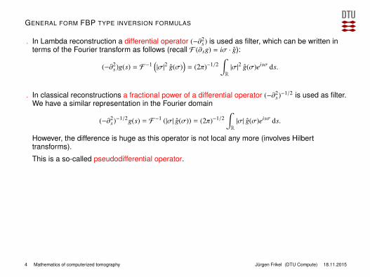
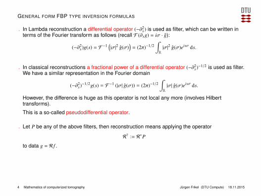
. In Lambda reconstruction a differential operator (−∂2s ) is used as filter, which can be written in
terms of the Fourier transform as follows (recall F (∂sg) = iσ · g):
(−∂2s )g(s) = F −1
(|σ|2 g(σ)
)= (2π)−1/2
∫R|σ|2 g(σ)eisσ ds.
. In classical reconstructions a fractional power of a differential operator (−∂2s )−1/2 is used as filter.
We have a similar representation in the Fourier domain
(−∂2s )−1/2g(s) = F −1 (|σ| g(σ)) = (2π)−1/2
∫R|σ| g(σ)eisσ ds.
However, the difference is huge as this operator is not local any more (involves Hilberttransforms).
This is a so-called pseudodifferential operator.
. Let P be any of the above filters, then reconstruction means applying the operator
R† := R∗Pto data g = R f .
. General FBP type reconstruction formulas use general pseudodifferential operators P asfilters.
4 Mathematics of computerized tomography Jurgen Frikel (DTU Compute) 18.11.2015
GENERAL FORM FBP TYPE INVERSION FORMULAS
. In Lambda reconstruction a differential operator (−∂2s ) is used as filter, which can be written in
terms of the Fourier transform as follows (recall F (∂sg) = iσ · g):
(−∂2s )g(s) = F −1
(|σ|2 g(σ)
)= (2π)−1/2
∫R|σ|2 g(σ)eisσ ds.
. In classical reconstructions a fractional power of a differential operator (−∂2s )−1/2 is used as filter.
We have a similar representation in the Fourier domain
(−∂2s )−1/2g(s) = F −1 (|σ| g(σ)) = (2π)−1/2
∫R|σ| g(σ)eisσ ds.
However, the difference is huge as this operator is not local any more (involves Hilberttransforms).
This is a so-called pseudodifferential operator.
. Let P be any of the above filters, then reconstruction means applying the operator
R† := R∗Pto data g = R f .
. General FBP type reconstruction formulas use general pseudodifferential operators P asfilters.
4 Mathematics of computerized tomography Jurgen Frikel (DTU Compute) 18.11.2015

GENERAL FORM FBP TYPE INVERSION FORMULAS
Since FBP type reconstructions are so easy to implement and since the yield very fastreconstructions, the are applied to all kinds of tomographic data, in particular to incomplete data
. Limited angle data
. Sparse angle data
. Interior data
. Exterior data
. . . .
What do we reconstruct?
5 Mathematics of computerized tomography Jurgen Frikel (DTU Compute) 18.11.2015
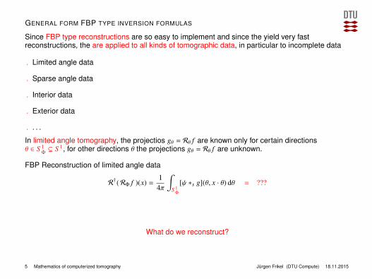
GENERAL FORM FBP TYPE INVERSION FORMULAS
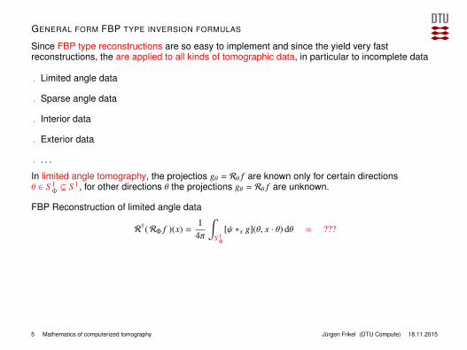
Since FBP type reconstructions are so easy to implement and since the yield very fastreconstructions, the are applied to all kinds of tomographic data, in particular to incomplete data
. Limited angle data
. Sparse angle data
. Interior data
. Exterior data
. . . .
In limited angle tomography, the projectios gθ = Rθ f are known only for certain directionsθ ∈ S 1
Φ( S 1, for other directions θ the projections gθ = Rθ f are unknown.
FBP Reconstruction of limited angle data
R†(RΦ f )(x) =1
4π
∫S 1
Φ
[ψ ∗s g](θ, x · θ) dθ = ???
What do we reconstruct?
5 Mathematics of computerized tomography Jurgen Frikel (DTU Compute) 18.11.2015
GENERAL FORM FBP TYPE INVERSION FORMULAS
Since FBP type reconstructions are so easy to implement and since the yield very fastreconstructions, the are applied to all kinds of tomographic data, in particular to incomplete data
. Limited angle data
. Sparse angle data
. Interior data
. Exterior data
. . . .
In limited angle tomography, the projectios gθ = Rθ f are known only for certain directionsθ ∈ S 1
Φ( S 1, for other directions θ the projections gθ = Rθ f are unknown.
FBP Reconstruction of limited angle data
R†(RΦ f )(x) =1
4π
∫S 1
Φ
[ψ ∗s g](θ, x · θ) dθ = ???
What do we reconstruct?
5 Mathematics of computerized tomography Jurgen Frikel (DTU Compute) 18.11.2015
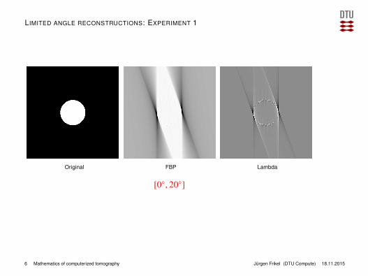
LIMITED ANGLE RECONSTRUCTIONS: EXPERIMENT 1
Original FBP Lambda
[0, 20]
6 Mathematics of computerized tomography Jurgen Frikel (DTU Compute) 18.11.2015

LIMITED ANGLE RECONSTRUCTIONS: EXPERIMENT 1
Original FBP Lambda
[0, 40]
6 Mathematics of computerized tomography Jurgen Frikel (DTU Compute) 18.11.2015

LIMITED ANGLE RECONSTRUCTIONS: EXPERIMENT 1
Original FBP Lambda
[0, 60]
6 Mathematics of computerized tomography Jurgen Frikel (DTU Compute) 18.11.2015

LIMITED ANGLE RECONSTRUCTIONS: EXPERIMENT 1
Original FBP Lambda
[0, 80]
6 Mathematics of computerized tomography Jurgen Frikel (DTU Compute) 18.11.2015

LIMITED ANGLE RECONSTRUCTIONS: EXPERIMENT 1
Original FBP Lambda
[0, 100]
6 Mathematics of computerized tomography Jurgen Frikel (DTU Compute) 18.11.2015

LIMITED ANGLE RECONSTRUCTIONS: EXPERIMENT 1
Original FBP Lambda
[0, 120]
6 Mathematics of computerized tomography Jurgen Frikel (DTU Compute) 18.11.2015

LIMITED ANGLE RECONSTRUCTIONS: EXPERIMENT 1
Original FBP Lambda
[0, 140]
6 Mathematics of computerized tomography Jurgen Frikel (DTU Compute) 18.11.2015

LIMITED ANGLE RECONSTRUCTIONS: EXPERIMENT 1
Original FBP Lambda
[0, 160]
6 Mathematics of computerized tomography Jurgen Frikel (DTU Compute) 18.11.2015
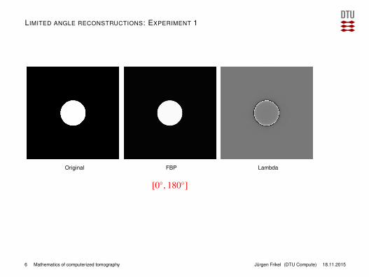
LIMITED ANGLE RECONSTRUCTIONS: EXPERIMENT 1
Original FBP Lambda
[0, 180]
6 Mathematics of computerized tomography Jurgen Frikel (DTU Compute) 18.11.2015

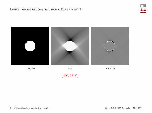
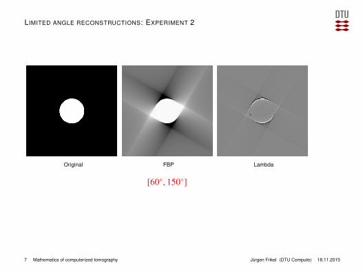
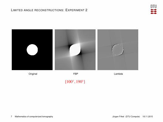
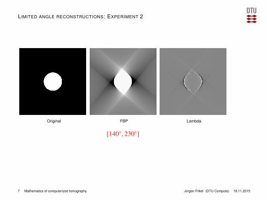
LIMITED ANGLE RECONSTRUCTIONS: EXPERIMENT 2
Original FBP Lambda
[0, 90]
7 Mathematics of computerized tomography Jurgen Frikel (DTU Compute) 18.11.2015
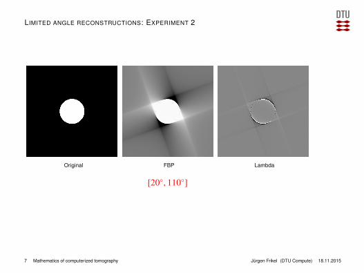
LIMITED ANGLE RECONSTRUCTIONS: EXPERIMENT 2
Original FBP Lambda
[20, 110]
7 Mathematics of computerized tomography Jurgen Frikel (DTU Compute) 18.11.2015
LIMITED ANGLE RECONSTRUCTIONS: EXPERIMENT 2
Original FBP Lambda
[40, 130]
7 Mathematics of computerized tomography Jurgen Frikel (DTU Compute) 18.11.2015
LIMITED ANGLE RECONSTRUCTIONS: EXPERIMENT 2
Original FBP Lambda
[60, 150]
7 Mathematics of computerized tomography Jurgen Frikel (DTU Compute) 18.11.2015

LIMITED ANGLE RECONSTRUCTIONS: EXPERIMENT 2
Original FBP Lambda
[80, 170]
7 Mathematics of computerized tomography Jurgen Frikel (DTU Compute) 18.11.2015
LIMITED ANGLE RECONSTRUCTIONS: EXPERIMENT 2
Original FBP Lambda
[100, 190]
7 Mathematics of computerized tomography Jurgen Frikel (DTU Compute) 18.11.2015

LIMITED ANGLE RECONSTRUCTIONS: EXPERIMENT 2
Original FBP Lambda
[120, 210]
7 Mathematics of computerized tomography Jurgen Frikel (DTU Compute) 18.11.2015
LIMITED ANGLE RECONSTRUCTIONS: EXPERIMENT 2
Original FBP Lambda
[140, 230]
7 Mathematics of computerized tomography Jurgen Frikel (DTU Compute) 18.11.2015
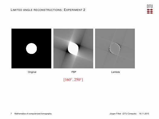
LIMITED ANGLE RECONSTRUCTIONS: EXPERIMENT 2
Original FBP Lambda
[160, 250]
7 Mathematics of computerized tomography Jurgen Frikel (DTU Compute) 18.11.2015

CHALLENGES IN LIMITED VIEW TOMOGRAPHY
Observations at a first glance:. Only certain features of the original object can be reconstructed
. Artifacts are generated
Goal:. Characterize image features that can be reliably reconstructed?
. Develop strategy to reduce artifacts?
Observations at a second glance:. Common characteristic features for both types of reconstructions are edges
. Information about edges is given in terms of projection directions
8 Mathematics of computerized tomography Jurgen Frikel (DTU Compute) 18.11.2015
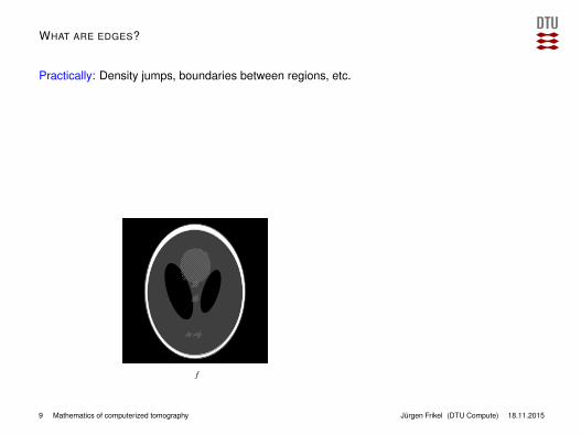
WHAT ARE EDGES?
Practically: Density jumps, boundaries between regions, etc.
Mathematically: Where the function is not smooth→ singularities.
Edges are local and oriented: What’s an appropriate mathematical framework?
9 Mathematics of computerized tomography Jurgen Frikel (DTU Compute) 18.11.2015
f
Singularities of f

WHAT ARE EDGES?
Practically: Density jumps, boundaries between regions, etc.
Mathematically: Where the function is not smooth→ singularities.
Edges are local and oriented: What’s an appropriate mathematical framework?
9 Mathematics of computerized tomography Jurgen Frikel (DTU Compute) 18.11.2015
f Singularities of f
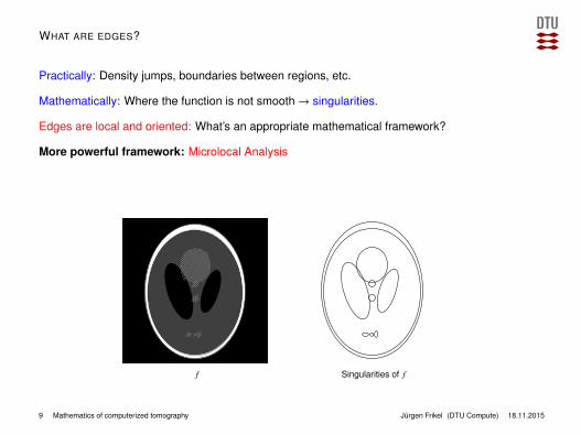

WHAT ARE EDGES?
Practically: Density jumps, boundaries between regions, etc.
Mathematically: Where the function is not smooth→ singularities.
Edges are local and oriented: What’s an appropriate mathematical framework?
Image processing: Location of singularities = locations of high gradient magnitude;
Direction of singularities = gradient directions
9 Mathematics of computerized tomography Jurgen Frikel (DTU Compute) 18.11.2015
f Singularities of f
WHAT ARE EDGES?
Practically: Density jumps, boundaries between regions, etc.
Mathematically: Where the function is not smooth→ singularities.
Edges are local and oriented: What’s an appropriate mathematical framework?
More powerful framework: Microlocal Analysis
9 Mathematics of computerized tomography Jurgen Frikel (DTU Compute) 18.11.2015
f Singularities of f

TODAY
. Global smoothness vs. decay of Fourier transform
. Singular locations
. Singular directions
. Wavefront sets: simultaneous description of singular locations and directions
. Examples
10 Mathematics of computerized tomography Jurgen Frikel (DTU Compute) 18.11.2015

GLOBAL SMOOTHNESS VS. DECAY OF FOURIER TRANSFORM
In what follows, we only consider real functions f : R2 → R.
The smoothness of any function f can be charachterized by means of the decay of its Fouriertransform f :
f ∈ Ck ⇔ f (ξ) = O(|ξ|−k) for |ξ| → ∞.In particular,
f ∈ C∞ ⇔ f (ξ) = O(|ξ|−k) for all k ∈ N.
Notation: A function which satisfies f (x) = O(|x|−k) for all k ∈ N is called rapidly decreasing. In allother cases slowly decreasing.
Definition
A function f which is not C∞ is called singular.
Equivalently, f is singular if the Fourier transform does not decay rapidly.
. Above relations can be proven by using the property F (Dα f ) = i|α|ξαF f
. Above relations also hold for distributions in D′ and S′
. If the Fourier transform of f has compact support (fastest decay one can imagine), then it canbe shown that the function f is analytic (Paley-Wiener)
. One can also use the above relations to define smoothness of order α ∈ R (Sobolev-Spaces)
11 Mathematics of computerized tomography Jurgen Frikel (DTU Compute) 18.11.2015

GLOBAL SMOOTHNESS VS. DECAY OF FOURIER TRANSFORM
Limitation:
. No information about locations or directions is provided.
. Global smoothness is related to a non-directional decay of the Fourier transform.
Example: Let f be a function which is smooth except at the point 0 ∈ R2, i.e. f ∈ C∞(R2 \ 0). Lety ∈ R2 be arbitrary and let fy(x) = f (x − y). Then
fy(ξ) = e−iξy f (ξ)
and hence ∣∣∣ fy(ξ)∣∣∣ =
∣∣∣ f (ξ)∣∣∣ .
That is, we can generate functions f and fy that have equal decay properties but arbitrarilydifferent locations of jums, discontinuities, etc..
Hence, the decay of the Fourier transform does not provide information about the location ofdiscontinuities.
12 Mathematics of computerized tomography Jurgen Frikel (DTU Compute) 18.11.2015

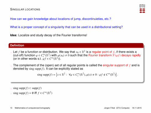
SINGULAR LOCATIONS
How can we gain knowledge about locations of jump, discontinuieties, etc.?
What is a proper concept of a singularity that can be used in a distributional setting?
Idea: Localize and study decay of the Fourier transforms!
Definition
. Let f be a function or distribution. We say that x0 ∈ R2 is a regular point of f , if there exists a(cut-off) function ϕ ∈ C∞c (R2) with ϕ(x0) , 0 such that the Fourier transform F (ϕ f ) decays rapidly(or in other words s.t. ϕ f ∈ C∞(R2)).
. The complement of the (open) set of all regular points is called the singular support of f and isdenoted by sing supp( f ). It can be explicitly stated as
sing supp( f ) =x ∈ R2 : ∀ϕ ∈ C∞c (R2), ϕ(x) , 0 : ϕ f < C∞(R2)
.
. sing supp( f ) ⊂ supp( f )
. sing supp( f ) = ∅ iff f ∈ C∞(R2)
13 Mathematics of computerized tomography Jurgen Frikel (DTU Compute) 18.11.2015

SINGULAR LOCATIONS
How can we gain knowledge about locations of jump, discontinuieties, etc.?
What is a proper concept of a singularity that can be used in a distributional setting?
Idea: Localize and study decay of the Fourier transforms!
Definition
. Let f be a function or distribution. We say that x0 ∈ R2 is a regular point of f , if there exists a(cut-off) function ϕ ∈ C∞c (R2) with ϕ(x0) , 0 such that the Fourier transform F (ϕ f ) decays rapidly(or in other words s.t. ϕ f ∈ C∞(R2)).
. The complement of the (open) set of all regular points is called the singular support of f and isdenoted by sing supp( f ).
It can be explicitly stated as
sing supp( f ) =x ∈ R2 : ∀ϕ ∈ C∞c (R2), ϕ(x) , 0 : ϕ f < C∞(R2)
.
. sing supp( f ) ⊂ supp( f )
. sing supp( f ) = ∅ iff f ∈ C∞(R2)
13 Mathematics of computerized tomography Jurgen Frikel (DTU Compute) 18.11.2015
SINGULAR LOCATIONS
How can we gain knowledge about locations of jump, discontinuieties, etc.?
What is a proper concept of a singularity that can be used in a distributional setting?
Idea: Localize and study decay of the Fourier transforms!
Definition
. Let f be a function or distribution. We say that x0 ∈ R2 is a regular point of f , if there exists a(cut-off) function ϕ ∈ C∞c (R2) with ϕ(x0) , 0 such that the Fourier transform F (ϕ f ) decays rapidly(or in other words s.t. ϕ f ∈ C∞(R2)).
. The complement of the (open) set of all regular points is called the singular support of f and isdenoted by sing supp( f ). It can be explicitly stated as
sing supp( f ) =x ∈ R2 : ∀ϕ ∈ C∞c (R2), ϕ(x) , 0 : ϕ f < C∞(R2)
.
. sing supp( f ) ⊂ supp( f )
. sing supp( f ) = ∅ iff f ∈ C∞(R2)
13 Mathematics of computerized tomography Jurgen Frikel (DTU Compute) 18.11.2015

SINGULAR DIRECTIONS
So far: Locations of singularities are given by the singular support and x ∈ sing supp f implies thatF (ϕ f ) decays slowly for any cut-off function ϕ(x0) , 0.
Can there exist directions along which F (ϕ f ) has rapid decay?
(Example with a line singularity suggests that this might be the case)
Definition
. Let f be a be compactly supported distribution. A direction ξ0 ∈ R2 \ 0 is called regular directionif there exists a conic neighborhood N of ξ0 such that f decays fast in N.
. The complement of the (open) set of all regular directions is called the frequency set of f and isdenoted by Σ( f ). It can be explicitly stated as
Σ( f ) =ξ ∈ R2 \ 0 : ∀conic neighb. N of ξ : f decays slowly in N
.
. Σ( f ) = ∅ iff f ∈ C∞(R2)
. Singular directions only exist if singularities exist and vice versa.
. For any compactly supported distribution f and any ϕ ∈ C∞c (R2) we have
Σ(ϕ f ) ⊂ Σ( f ),
i.e., multiplication by compactly supported smooth function does not add singular directions.
14 Mathematics of computerized tomography Jurgen Frikel (DTU Compute) 18.11.2015
LOCATION AND DIRECTION OF A SINGULARITY
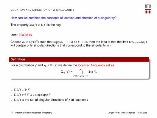
How can we combine the concepts of location and direction of a singularity?
The property Σ(ϕ f ) ⊂ Σ( f ) is the key.
Idea: ZOOM IN
Choose ϕk ∈ C∞c (R2) such that supp(ϕk)→ x as k → ∞, then the idea is that the limit limk→∞ Σ(ϕ f )will contain only singular directions that correspond to the singularity in x.
Definition
For a distribution f and x0 ∈ R2( f ) we define the localized frequency set as
Σx0 ( f ) =⋂
ϕ∈C∞c ,ϕ(x0),0
Σ(ϕ f ).
. Σx( f ) ⊂ Σ( f )
. Σx( f ) , ∅ iff x ∈ sing supp( f )
. Σx( f ) is the set of singular directions of f at location x
15 Mathematics of computerized tomography Jurgen Frikel (DTU Compute) 18.11.2015
LOCATION AND DIRECTION OF A SINGULARITY
How can we combine the concepts of location and direction of a singularity?
The property Σ(ϕ f ) ⊂ Σ( f ) is the key.
Idea: ZOOM IN
Choose ϕk ∈ C∞c (R2) such that supp(ϕk)→ x as k → ∞, then the idea is that the limit limk→∞ Σ(ϕ f )will contain only singular directions that correspond to the singularity in x.
Definition
For a distribution f and x0 ∈ R2( f ) we define the localized frequency set as
Σx0 ( f ) =⋂
ϕ∈C∞c ,ϕ(x0),0
Σ(ϕ f ).
. Σx( f ) ⊂ Σ( f )
. Σx( f ) , ∅ iff x ∈ sing supp( f )
. Σx( f ) is the set of singular directions of f at location x
15 Mathematics of computerized tomography Jurgen Frikel (DTU Compute) 18.11.2015

THE WAVEFRONT SET
Definition
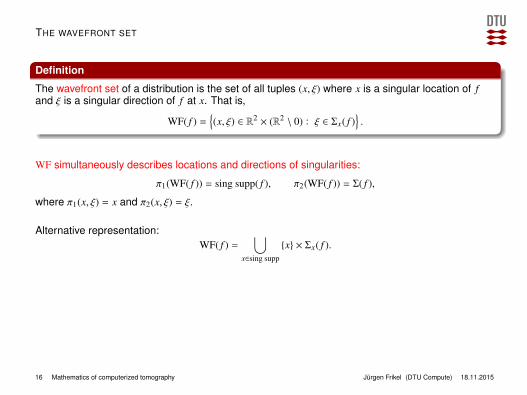
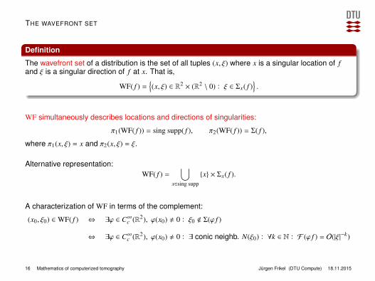
The wavefront set of a distribution is the set of all tuples (x, ξ) where x is a singular location of fand ξ is a singular direction of f at x. That is,
WF( f ) =(x, ξ) ∈ R2 × (R2 \ 0) : ξ ∈ Σx( f )
.
WF simultaneously describes locations and directions of singularities:
π1(WF( f )) = sing supp( f ), π2(WF( f )) = Σ( f ),
where π1(x, ξ) = x and π2(x, ξ) = ξ.
Alternative representation:WF( f ) =
⋃x∈sing supp
x × Σx( f ).
A characterization of WF in terms of the complement:
(x0, ξ0) ∈WF( f ) ⇔ ∃ϕ ∈ C∞c (R2), ϕ(x0) , 0 : ξ0 < Σ(ϕ f )
⇔ ∃ϕ ∈ C∞c (R2), ϕ(x0) , 0 : ∃ conic neighb. N(ξ0) : ∀k ∈ N : F (ϕ f ) = O(|ξ|−k)
16 Mathematics of computerized tomography Jurgen Frikel (DTU Compute) 18.11.2015

THE WAVEFRONT SET
Definition
The wavefront set of a distribution is the set of all tuples (x, ξ) where x is a singular location of fand ξ is a singular direction of f at x. That is,
WF( f ) =(x, ξ) ∈ R2 × (R2 \ 0) : ξ ∈ Σx( f )
.
WF simultaneously describes locations and directions of singularities:
π1(WF( f )) = sing supp( f ), π2(WF( f )) = Σ( f ),
where π1(x, ξ) = x and π2(x, ξ) = ξ.
Alternative representation:WF( f ) =
⋃x∈sing supp
x × Σx( f ).
A characterization of WF in terms of the complement:
(x0, ξ0) ∈WF( f ) ⇔ ∃ϕ ∈ C∞c (R2), ϕ(x0) , 0 : ξ0 < Σ(ϕ f )
⇔ ∃ϕ ∈ C∞c (R2), ϕ(x0) , 0 : ∃ conic neighb. N(ξ0) : ∀k ∈ N : F (ϕ f ) = O(|ξ|−k)
16 Mathematics of computerized tomography Jurgen Frikel (DTU Compute) 18.11.2015

EXAMPLES
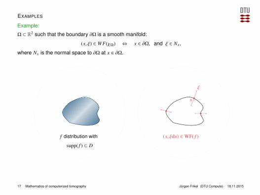
Example:
Ω ⊂ R2 such that the boundary ∂Ω is a smooth manifold:
(x, ξ) ∈ WF(χΩ) ⇔ x ∈ ∂Ω, and ξ ∈ Nx,
where Nx is the normal space to ∂Ω at x ∈ ∂Ω.
17 Mathematics of computerized tomography Jurgen Frikel (DTU Compute) 18.11.2015

EXAMPLES
Example:
Ω ⊂ R2 such that the boundary ∂Ω is a smooth manifold:
(x, ξ) ∈ WF(χΩ) ⇔ x ∈ ∂Ω, and ξ ∈ Nx,
where Nx is the normal space to ∂Ω at x ∈ ∂Ω.
17 Mathematics of computerized tomography Jurgen Frikel (DTU Compute) 18.11.2015
EXAMPLES
Example:
Ω ⊂ R2 such that the boundary ∂Ω is a smooth manifold:
(x, ξ) ∈ WF(χΩ) ⇔ x ∈ ∂Ω, and ξ ∈ Nx,
where Nx is the normal space to ∂Ω at x ∈ ∂Ω.
f distribution with
supp( f ) ⊂ D
bx
ξ
bb
(x, ξdx) ∈WF( f )
17 Mathematics of computerized tomography Jurgen Frikel (DTU Compute) 18.11.2015

EXAMPLES
Example:
Ω ⊂ R2 such that the boundary ∂Ω is a smooth manifold:
(x, ξ) ∈ WF(χΩ) ⇔ x ∈ ∂Ω, and ξ ∈ Nx,
where Nx is the normal space to ∂Ω at x ∈ ∂Ω.
17 Mathematics of computerized tomography Jurgen Frikel (DTU Compute) 18.11.2015
What happens at crossings and corners?
If x is a corner or a crossing singularity (or of similar nature), Σx( f ) = R2 \ 0.
f
bx
ξ
(x, ξ) ∈WF( f )
Singularities of f

PSEUDODIFFERENTIAL OPERATORS ΨDO’S
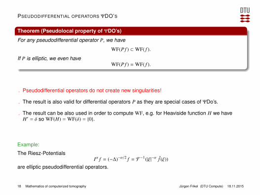
Theorem (Pseudolocal property of ΨDO’s)
For any pseudodifferential operator P, we have
WF(P f ) ⊂WF( f ).
If P is elliptic, we even haveWF(P f ) = WF( f ).
. Pseudodifferential operators do not create new singularities!
. The result is also valid for differential operators P as they are special cases of ΨDo’s.
. The result can be also used in order to compute WF, e.g. for Heaviside function H we haveH′ = δ so WF(H) = WF(δ) = 0.
Example:
The Riesz-PotentialsIα f = (−∆)−α/2 f = F −1(|ξ|−α f (ξ))
are elliptic pseudodifferential operators.
18 Mathematics of computerized tomography Jurgen Frikel (DTU Compute) 18.11.2015

PSEUDODIFFERENTIAL OPERATORS ΨDO’S
Theorem (Pseudolocal property of ΨDO’s)
For any pseudodifferential operator P, we have
WF(P f ) ⊂WF( f ).
If P is elliptic, we even haveWF(P f ) = WF( f ).
. Pseudodifferential operators do not create new singularities!
. The result is also valid for differential operators P as they are special cases of ΨDo’s.
. The result can be also used in order to compute WF, e.g. for Heaviside function H we haveH′ = δ so WF(H) = WF(δ) = 0.
Example:
The Riesz-PotentialsIα f = (−∆)−α/2 f = F −1(|ξ|−α f (ξ))
are elliptic pseudodifferential operators.
18 Mathematics of computerized tomography Jurgen Frikel (DTU Compute) 18.11.2015
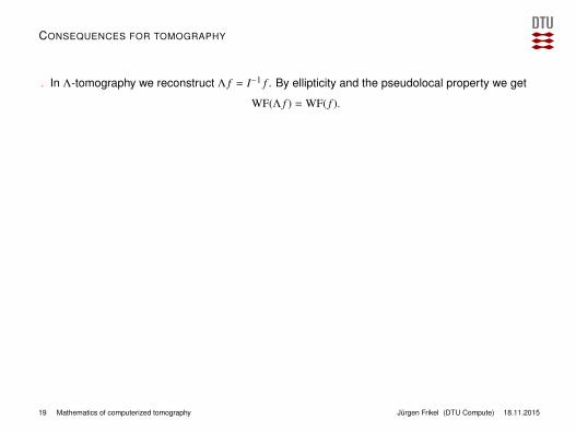
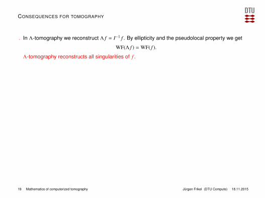
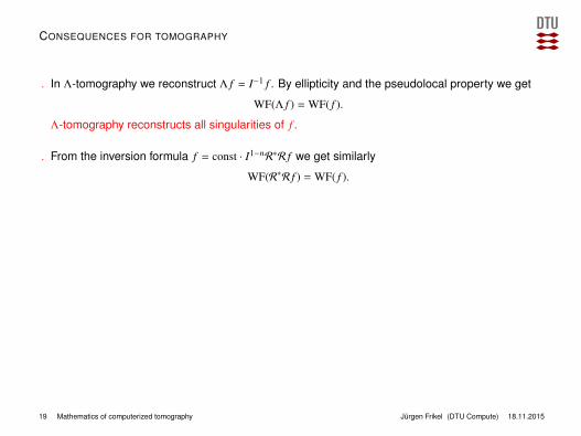
CONSEQUENCES FOR TOMOGRAPHY
. In Λ-tomography we reconstruct Λ f = I−1 f . By ellipticity and the pseudolocal property we get
WF(Λ f ) = WF( f ).
Λ-tomography reconstructs all singularities of f .
. From the inversion formula f = const · I1−nR∗R f we get similarly
WF(R∗R f ) = WF( f ).
. Although singularities are differently pronounced in f , R∗R f and Λ f , we have
WF( f ) = WF(R∗R f ) = WF(Λ f ).
WF does not quantify the strength of singularities. To quantify the strength of singularities, arefined notion of the wavefront set can be defined (Sobolev wavefront set).
. For general FBP type reconstruction operators R∗P with general pseudodifferential operators Pas filters, a minimum requirement on the filter can be formulated as
WF(R∗PR f ) != WF( f ).
In general, this is not even if P is elliptic.
19 Mathematics of computerized tomography Jurgen Frikel (DTU Compute) 18.11.2015

Thanks!
Next week: Microlocal analysis in limited angle tomography
20 Mathematics of computerized tomography Jurgen Frikel (DTU Compute) 18.11.2015


