Lectures on Numerical Methods In Bifurcation Problemspubl/ln/tifr79.pdf · Lectures on Numerical...

Lectures onNumerical Methods In Bifurcation Problems

By

H.B. Keller

Lectures delivered at theIndian Institute Of Science, Bangalore

under the

T.I.F.R.-I.I.Sc. Programme In Applications Of

Mathematics

Notes by

A.K.Nandakumaran and Mythily Ramaswamy

Published for theTata Institute Of Fundamental Research

Springer-VerlagBerlin Heidelberg New York Tokyo

AuthorH.B. Keller

Applied Mathematics 217-50California Institute of Technology

Pasadena, California 91125U.S.A.

c©Tata Institute Of Fundamental Research, 1986

ISBN 3-540-20228-5 Springer-verlag, Berlin, Heidelberg,New York. Tokyo

ISBN 0-387-20228-5 Springer-verlag, New York. Heidelberg.Berlin. Tokyo

No part of this book may be reproduced in anyform by print, microfilm or any other means with-out written permission from the Tata Institute ofFundamental Research, Colaba, Bombay-400 005.

Printed byINSDOC Regional Centre.

Indian Institute of Science Campus,Bangalore-560 012

and published by H.Goctzc, Springer-Verlag,Heidelberg, West Germany

Printed In India

Preface

These lectures introduce the modern theory of continuationor path fol-lowing in scientific computing. Almost all problem in science and tech-nology contain parameters. Families or manifolds of solutions of suchproblems, for a domain of parameter variation, are of prime interest.Modern continuation methods are concerned with generatingthese so-lution manifolds. This is usually done by varying one parameter at atime - thus following a parameter path curve of solutions.

We present a familiar, interesting and simple example in Chapter 1which displays most of the basic phenomena that occur in morecomplexproblems. In Chapter 2 we examine some local continuation methods,bases mainly on the implicit function theorem. We go on to introduceconcepts of global continuation, degree theory and homotopy invari-ance with several important applications in Chapter 3. In Chapter 4,we discuss practical path following procedures, and introduce folds orlimit point singularities. Pseudo-arclength continuation is also intro-duced here to circumvent the simple fold difficulties. General singularpoints and bifurcations are briefly studied in Chapter 5 where branchswitching and (multiparameter) fold following are discussed. We alsovery briefly indicate how periodic solutions path continuation and Hopfbifurcations are Incorporated into our methods. Finally inChapter 6, wediscuss two computational examples and some details of general meth-ods employed in carrying out such computations.

This material is based on a series of lectures I presented at the Tatainstitute of Fundamental Research in Bangalore, India during Decem-ber 1985, and January 1986. It was a most stimulating and enjoyable

iii

iv

experienced for me, and the response and interaction with the audiencewas unusually rewarding. The lecture notes were diligentlyrecordedand written up by Mr. A.K. Nandakumar of T.I.F.R., Bangalore. Thefinal chapter was mainly worked out with Dr. Mythily Ramaswamy ofT.I.F.R. Ramaswamy also completely reviewed the entire manuscript,corrected many of the more glaring errors and made many otherim-provements. Any remaining errors are due to me. The iteration to con-verge on the final manuscript was allowed only one step due to the dis-tance involved. The result, however, is surprisingly closeto parts of myoriginal notes which are being independently prepared for publicationin a more extend form.

I am most appreciative to the Tata Institute of Fundamental Researchfor the opportunity to participate in their program. I also wish to thankthe U.S. Department of Energy and the U.S.Army Research Office whohave for years sponsored much of the research that has resulted in theselectures under the grants: 0E-AS03-7603-00767 and DAAG29-80-C-0041.

Herbert B. KellerPasadena, CaliforniaDecember 29, 1986

Contents

1 Basic Examples 11.1 Introduction . . . . . . . . . . . . . . . . . . . . . . . . 11.2 Examples (population dynamics) . . . . . . . . . . . . . 2

2 Local continuation methods 152.1 Introduction . . . . . . . . . . . . . . . . . . . . . . . . 152.2 Contraction Mapping Theorem . . . . . . . . . . . . . . 152.4 Contracting Ball Lemma . . . . . . . . . . . . . . . . . 162.5 Fundamental Theorem of Calculus . . . . . . . . . . . . 172.7 Implicit Function Theorem . . . . . . . . . . . . . . . . 172.14 Step Length Bound . . . . . . . . . . . . . . . . . . . . 202.18 Approximate Implicit Function Theorem . . . . . . . . . 232.20 Step Length Bound . . . . . . . . . . . . . . . . . . . . 242.22 Other Local Rootfinders . . . . . . . . . . . . . . . . . 262.23 Newton-Kantorovich Theorem . . . . . . . . . . . . . . 272.24 Newton Convergence Theorem . . . . . . . . . . . . . . 282.27 Predictor-Solver Methods . . . . . . . . . . . . . . . . . 302.29 Lemma . . . . . . . . . . . . . . . . . . . . . . . . . . 35

3 Global continuation theory 373.1 Introduction . . . . . . . . . . . . . . . . . . . . . . . . 373.2 Sard’s Theorem . . . . . . . . . . . . . . . . . . . . . . 383.3 Examples . . . . . . . . . . . . . . . . . . . . . . . . . 393.4 Solution sets for Regular Values . . . . . . . . . . . . . 403.5 Lemma (Finite Set of Solutions) . . . . . . . . . . . . . 40

v

vi Contents

3.6 Lemma (Global Solution Paths) . . . . . . . . . . . . . 413.7 Degree Theory . . . . . . . . . . . . . . . . . . . . . . 433.8 Definition . . . . . . . . . . . . . . . . . . . . . . . . . 443.9 Definition . . . . . . . . . . . . . . . . . . . . . . . . . 453.10 Definition . . . . . . . . . . . . . . . . . . . . . . . . . 453.11 Theorem (Homotopy Invariance of the Degree) . . . . . 463.13 Brouwer Fixed Point Theorem . . . . . . . . . . . . . . 513.14 Theorem . . . . . . . . . . . . . . . . . . . . . . . . . . 523.15 Periodic Solution Theorem . . . . . . . . . . . . . . . . 523.17 Theorem (Bifurcation Test) . . . . . . . . . . . . . . . . 543.18 Global Homotopies and Newton’s Method . . . . . . . . 563.22 Boundary conditions (Smale) . . . . . . . . . . . . . . . 583.24 Theorem . . . . . . . . . . . . . . . . . . . . . . . . . . 60

4 Practical procedures in computing paths 634.1 Introduction . . . . . . . . . . . . . . . . . . . . . . . . 634.5 Pseudoarclength Continuation . . . . . . . . . . . . . . 664.11 Bordering Algorithm . . . . . . . . . . . . . . . . . . . 68

5 Singular Points and Bifurcation 775.1 Introduction . . . . . . . . . . . . . . . . . . . . . . . . 775.3 Definition . . . . . . . . . . . . . . . . . . . . . . . . . 775.8 Bifurcation Theorem . . . . . . . . . . . . . . . . . . . 825.10 Definition . . . . . . . . . . . . . . . . . . . . . . . . . 845.13 Continuation Past Simple Singular Points . . . . . . . . 865.15 Properties at Folds and Bifurcation Points on Paths . . .885.21 Exchange of Stability . . . . . . . . . . . . . . . . . . . 925.26 Switching Branches at Bifurcation Points . . . . . . . . 935.27 Multi Parameter Problems (Fold Following) . . . . . . . 985.41 Paths of Periodic Solutions and Hopf Bifurcation . . . . 103

6 Numerical Examples 1116.1 Introduction . . . . . . . . . . . . . . . . . . . . . . . . 1116.2 Problems and Difference Schemes . . . . . . . . . . . . 1126.16 Algorithm and Tests . . . . . . . . . . . . . . . . . . . . 1176.17 Numerical Examples . . . . . . . . . . . . . . . . . . . 119

Chapter 1

Basic Examples

1.1 Introduction1

Our aim in these lectures is to study constructive methods for solvingnonlinear systems of the form :

(1.1) G(u, λ) = 0,

whereλ is a possibly multidimensional parameter andG is a smoothfunction or operator from a suitable function space into itself. Fre-quently we will work in finite dimensional spaces. In this introductorychapter we present two examples from population dynamics and studythe behaviour of solutions regarding bifurcation, stability and exchangeof stability. Second chapter describes a local continuation method andusing this we will try to obtain global solution of (1.1). Theimportanttool for studying this method is theimplicit function theorem. We willalso present various predictor - solver methods. The third chapter dealswith global continuation theory. Degree theory and some of its appli-cations are presented there. Later in that chapter we will study globalhomotopies and Newton methods for obtaining solutions of the equation(1.1).

In the fourth chapter, we describe a practical procedure forcomput-ing paths and introduce the method of arclength continuation. Using thebordering algorithm presented in that chapter, we can compute paths in

1

2 1. Basic Examples

an efficient way. In chapter 5, we will study singular points and bifur-cation. A clear description of various methods of continuation past sin-gular points, folds, branch switching at bifurcations points is presented2

in that chapter. We also study multiparameter problems, Hopfbifurca-tions later in that chapter. The final chapter presents some numericalresults obtained using some of the techniques presented in the previouschapters.

1.2 Examples (population dynamics)

We start with a simple, but important example from population dynam-ics (see [11], [24]). Letu(t) denote the populations density in a particularregion, at timet. The simplest growth law states that therate of changeof population is proportional to the existing density, thatis:

(1.3)dudt= βu,

whereβ is the reproduction rate. The solution for this problem is givenby

(1.4) u(t) = ueβ(t−t), u = u(t).

Note thatu(t) → ∞ as t → ∞. This means that population growsindefinitely with time. Obviously, we know that such situation is notpossible in practice. Henceβ cannot be a constant. It must decrease asu increases. Thus as a more realistic model, we letβ be a function ofu,say linear inu :

(1.5) β = β1(1−uu1

).

Hereβ1 > 0, is the ideal reproduction rate, andu1 is the maximaldensity that can be supported in the given environment.

Note that ifu > u1 thenβ < 0 so thatu(t) decays. On the other hand,3

if u < u1 thenu(t) grows as time increases. The solutions curve withβ

as above is sketched in figure 1.1; it is:

(1.6) u(t) =uu1eβ1t

(u1 − u) + ueβ1t, where u = u(0).

1.2. Examples (population dynamics) 3

Figure 1.1:

We now consider the more general case, in which coupling withanexternal population density, sayu, is allowed. Specifically we take

(1.7)dudt= β1(1−

uu1

)u+ αo(u − u)

where,

β1 = ideal reproduction rate(> 0),

u1 = maximal density,

u = exterior density,

α = flow rate (α ≥ 0 orα ≤ 0).

Naturally, the population of a particular region may dependuponthe population of the neighbouring regions. If the populations of theexterior is less, then species may move to that region (α > 0) and vice 4

versa (α < 0). The termα(u − u) accounts for this behaviour.We scale (1.7) by setting

λ1 =β1 − αβ1

u1,

λ1 =αβ1

u1u,

t = tu1

β1.

4 1. Basic Examples

Then we have

(1.8)dudt= G(u, λ) ≡ −u2

+ λ1u+ λ2.

Hereλ = (λ1, λ2) denotes the two independent parametersλ1 andλ2.

STEADY STATES: The steady state are solutions of

G(u, λ) = 0.

These solutions are :

(1.9) u± =λ1

2+

√(λ1

2)2 + λ2

These solutions are distinct unless

(1.10) λ2 = −(λ1

2)2.

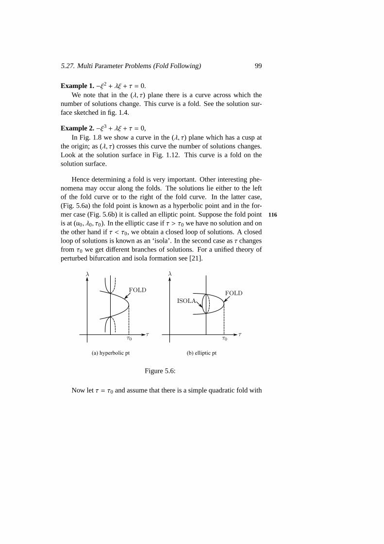
Along this curve in the (λ1, λ2) plane,Gu(u, λ) = 0. This curveis known as a fold (sometimes it is called the bifurcation set) and thenumber of solutions changes as one crosses this curve (See Fig. 1.2).

FoldO

ne so

lutio

n

No

Real solution

two

solutions

Figure 1.2:5

We examine three distinct cases :

(i) λ2 = 0 (ii) λ2 > 0 (iii) λ2 < 0.


(i) λ2 = 0 : The solutions are two straight lines given byu ≡ 0and u = λ1. They intersect at the origin. The origin is thus abifurcation point , where two distinct solution branches intersect.

(ii) λ2 > 0 : In this case, there are two solutionsu+ andu−, arcs of thehyperbola, whose asymptotes are given byu = 0 andu = λ1.

(iii) λ2 < 0 : In this case, a real solution exists only if|λ1| >√−4λ2.

They are the hyperbolae conjugate to those of case (ii)(See Fig. 1.3).

Figure 1.3:

The solution surfaces in the space (u, λ1, λ2) is sketched is Fig. 1.4.6It is clearly a saddle surface with saddle point at the origin. As we seelater on, the cases (ii) and (iii) are example of perturbed bifurcation.

Figure 1.4:

6 1. Basic Examples

STABILITY : To examine the stability of these states we note that (1.8)can be written as:

(1.11)dudt= −(u− u+)(u− u−).

Then it clearly follows that :

(1.12)dudt

< 0 if u < u− < u+> 0 if u− < u < u+< 0 if u− < u+ < u.

This means thatu decreases when it is in the semi-infinite intervalsu < u− andu+ < u. It increases inu− < u < u+. Hence it follows thatu+ is always stable and thatu− is always unstable. Note that the trivial7

solutionu ≡ 0 consists ofu+ for λ1 < 0. andu− for λ1 > 0. Thus inthe bifurcation case,λ2 = 0, the phenomenon of exchange of stabilityoccurs asλ1 changes sign. That is the branch which is stable changes asλ1 passes though the bifurcation valueλ1 = 0.

Figure 1.5: (λ2 = 0) Figure 1.6: (λ2 > 0)


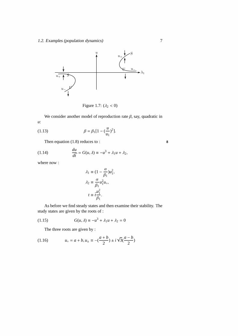
Figure 1.7: (λ2 < 0)

We consider another model of reproduction rateβ, say, quadratic inu:

(1.13) β = β1[1 − (uu1

)2].

Then equation (1.8) reduces to : 8

(1.14)dudt= G(u, λ) ≡ −u3

+ λ1u+ λ2,

where now :

λ1 ≡ (1−α

β1)u2

1,

λ2 ≡α

β1u2

1u,

t ≡ tu2

1

β1.

As before we find steady states and then examine their stability. Thestudy states are given by the roots of :

(1.15) G(u, λ) ≡ −u3+ λ1u+ λ2 = 0

The three roots are given by :

(1.16) u = a+ b, u± ≡ −(a+ b

2) ± i√

3(a− b

2)

8 1. Basic Examples

where,

a = (λ2

2+ (

λ22

4−λ3

1

27)1/2)1/3

b = (λ2

2+ (

λ22

4−λ3

1

27)1/2)1/3

In particular either we have 3 real roots or one real root. Clearly, if

λ22 −

427λ3

1 > 0, the there will one real root and two conjugate complex

roots. Ifλ22 −

427λ3

1 = 0 then there will be three real roots of which two

are equal. Ifλ22 −

427λ3

1 < 0 then there will be three distinct real roots.

This can be seen as follows. Put

a = (a1 + ib1)1/3, thenb = (a1 − ib1)1/3.

By changinga1 + ib1 to polar co-ordinates, we can easily see thata+ b is a real number anda− b is purely imaginary. Now9

Gu(u, λ) = −3u2+ λ1.

Combining (1.15) together withGu(u, λ) = 0 we get

(1.17) λ31 =

274λ2

2.

This curve in the (λ1, λ2) plane represents afold where the two realroots become equal; across the fold they become complex. Again notethat across the fold (Bifurcation Set) the number of solutions changes.Observe that atλ2 = 0, the solution contains the trivial branchu = 0and the parabola whose branches areu± = ±

√λ1 which passes through

the origin. Hence the origin is abifurcation point. We call this con-figuration apitchfork bifurcation. For λ2 > 0 or λ2 < 0 there is nobifurcation. The fold has a cusp at the origin and is sketchedin Fig. 1.8.


2 solutio

ns

3 solutions

1 solution

Fold

Figure 1.8:

Now we will analyse the stability results in different cases. (1.14)can be written as :

(1.18)dudt= −(u− uo)(u− u+)(u− u−).

10

(i) λ2 = 0: The dynamic in this case are simply generated by,

(1.19)dudt= −u(u−

√λ1)(u+

√λ1),

and hence we see that:

(1.20)dudt

> 0 if u < −√λ1 < 0,

< 0 if −√λ1 < u < 0,

> 0 if 0 < u <√λ1,

< 0 if 0 <√λ1 < u.

Thusuo is stable forλ1 < 0 and it becomes unstable asλ1 changessign toλ1 > 0. In this latter range bothu± are stable.

(ii) λ2 > 0: Then

(1.21)dudt

> O if u < uo,

> 0 if uo < u < u−,

> 0 if u− < u < u+,

< 0 if u+ < u.

10 1. Basic Examples

(iii) λ2 < 0: In a similar way the stability results can be obtained herealso.

The stability results are indicated in figures 1.9, 1.10, 1.11. Thesolution surface is sketched in figure 1.12.

Figure 1.9: (λ2 = 0) Figure 1.10: (λ2 > 0)11

Figure 1.11: (λ2 < 0)

Figure 1.12:


Now we present one more example from population dynamics, in12

which there are two species in the same region. We know that there is aconstant struggle for survival among different species of animals livingin the same environment. For example, consider a region inhabited byfoxes and rabbits. The foxes eat rabbits and hence this population growsas the rabbits diminish. But when the population of rabbits decreasessufficiently the fox population must decrease (due to hunger). Asa re-sult the rabbits are relatively safe and their population starts to increaseagain. Thus we can expect a repeated cycle of increase and decrease ofthe two species, i.e. a periodic solution. To model this phenomenon, wetake the coupled system :

ut = βu[1 − (uu1

)2 − (vv1

)2] u+ αu(uo − u) − γuv,

vt = βv[1 − (uu1

)2 − (vv1

)2] v+ αv(vo − v) + γvu.(1.22)

Hereu is prey density and ˜v is predator density and ˜γu > 0, γv > 0.We have also assumed that both species compete for the same “vege-tation” so that each of their effective reproduction rates are diminishedtogether. To scale we now introduce:

u ≡ uu1, v ≡ v

v1,

uo ≡uo

u1, vo ≡

vo

v1

γu ≡ γuv1

u1, γv ≡ γv

u1

v1.

(1.23)

But to simplify we will consider only a special case in which theeight parameters are reduced to one by setting : 13

βu = βv = γu = γv = 1,

uo = vo = 0,

λ = 1− αu = 1− αv.

(1.24)

Note that hereλ is similar to the parameterλ1 of our previous ex-ample.


Now (1.24) reduces to the system :

(1.25)

(uv

)

t=

(λ −11 λ

) (uv

)− (u2

+ v2)

(uv

).

Note that(uv

)=

(00

), the trivial solution is valid for allλ. First we

consider a small perturbation(δuδv

)about the trivial solution

(00

). This

satisfies the linearized problem :

(1.26)

(δu

δv

)

t= A

(δu

δv

), where A =

(λ −11 λ

).

The eigenvalues ofA are given by :

(1.27) n± = λ ± i.

These eigenvalues are distinct and hence the solutions of the lin-earized problem must have the form :

δu = a1en+t+ a2en−t

δv = b1en+t+ b2en−t(1.28)

For all λ < 0, we thus have thatδu, δv → 0 ast → ∞. Hence thetrivial state is a stable solution. On the other hand, ifλ > 0, thenδu, δvgrow exponentially ast → ∞ and the trivial state is unstable forλ > 0.Observe that there is an exchange of stability asλ crosses the origin.14

For λ = 0 we get periodic solution of the linearized problem. Indeedwe now show that the exact nonlinear solutions have similar feature, butthat stable periodic solutions exist for allλ > 0.

Introduce polar co-ordinates in the (u, v) plane :

u = ρ cosθ, v = ρ sinθ,

u2+ v2= ρ2, tanθ =

vu.

(1.29)

The system (1.25) becomes, withρ ≥ 0:

ρ cos θ − ρθ sin θ = λρ cos θ − ρ sin θ − ρ3 cos θ,

ρ sin θ + ρθ cos θ = ρ cos θ + λρ sin θ − ρ3 cos θ.(1.30)


Appropriate combinations of these equations yield :

ρ = λρ − ρ3= ρ(λ − ρ2),(1.31)

θ = +1.(1.32)

Thusθ(t) = θ0 + t, whereθ0 is an arbitrary constant. From (1.31),

for λ > 0,ρ(t) is given byρ(t)(τ + ρ(t)τ − ρ(t)

)1/2= Ceλt, whereτ =

√λ andC

is an arbitrary constant. Forλ < 0, ρ(t) is given byρ(t)

√ρ2(t) − λ

= Ceλt.

We now examine two casesλ > 0 andλ < 0.

(i) λ < 0: Thenρ < 0 for all t. This impliesρ(t) decreases to 0 astincreases.

(ii) λ > 0: Here we have to consider 3 possibilities for the state at any 15

time to:

(iia) ρ(to) < ρcr ≡√λ

Now ρ(t) < 0 andρ(t) increases towardsρcr ast ↑ ∞

(iib) ρ(to) > ρcr

Now ρ(t) < 0 andρ(t) decreases towardsρcr ast ↑ ∞

(iic) ρ(to) = ρcr

Now ρ(t) ≡ 0 and we have the periodic solution :

u = ρcr cos (θo + t), v = ρcr sin (θo + t).

These solutions are unique upto a phase,θo. The “solution surface”in the (u, v, λ) space contains the trivial branch and a paraboloid, whichis sketched in Fig. 1.13


Figure 1.13:

This is a standard example of Hopf bifurcation - a periodic solutionbranches off from the trivial steady state asλ crosses a critical value,in this caseλ = 0. The important fact is that for the complex pair16

of eigenvaluesρ±(λ), the real part crosses zero and as we shall see ingeneral, it is this behaviour which leads to Hopf bifurcation.

We have seen the change in the number of solutions across foldsand two types of steady state bifurcations and one type of periodic bi-furcation in our special population dynamics example. We shall nowstudy much more general steady states and time dependant problems inwhich essentially these same phenomena occur. Indeed they are in asense typical of the singular behaviour which occurs as parameters arevaried in nonlinear problems. Of course even more varied behaviour ispossible as we shall see (see [4], [13], [23], for example). One of thebasic tools in studying singular behaviour is to reduce the abstract caseto simple algebraic forms similar to those we have already studied (orgeneralizations).

Chapter 2

Local continuation methods

2.1 Introduction17

We will use a local continuation method to get global solutions of thegeneral problem:

(2.1) G(u, λ) = 0

Suppose we are given a solution (uo, λo) of (2.1). The idea of localcontinuation is to find a solution at (λo

+ δλ) for a small perturbationδλ. Then perhaps, we can proceed step by step, to get a global solu-tion. The basic tool for this study is the implicit function theorem.Thecontinuation method may fail at some step because of the existence ofsingularities on the curve (for example folds or bifurcation points). Nearthese points there exist more than one solution and the implicit functiontheorem isnot valid.

First we recall a basic theorem which is the main tool in proving theimplicit function theorem.

2.2 Contraction Mapping Theorem

Let B be a Banach space and F: B→ B satisfy:

(2.2)(a) F(Ω) ⊂ Ω for some closed subsetΩ ⊂ B.(b) ‖F(u) − F(v)‖ ≤ θ‖u − v‖ for someθ ∈

(0, 1) and for all u, v ∈ Ω.

15

16 2. Local continuation methods

Then the equation18

u = F(u)

has one and only one solution u∗ ∈ Ω. This solution is the limit of anysequenceuU , U = 0, 1, 2, . . . generated by

(2.3)(a) uo ∈ Ω, arbitrary;(b) uU+1 = F(uU),U = 0, 1, 2, . . . . . .

The convergence is such that:

(2.3) (c)‖u∗ − uU‖ ≤θU

1− θ‖uo − F(u0)‖ ≡

θU

1− θ‖u0 − u1‖.

Proof. Well known

We will state another lemma which shows how to find a setΩ, inwhich the conditions of theorem (2.2) hold.

2.4 Contracting Ball Lemma

Letρ > 0, θ ∈ (0, 1) be such that for some uo ∈ B, F satisfies:

(2.4)(a) ‖uo − F(uo)‖ ≤ (1− θ)ρ.(b) ‖F(u) − F(v)‖ ≤ θ‖u− v‖ for all , u, v ∈ Bρ(uo).

where

Bρ(uo) = u ∈ B : ‖u− uo‖ ≤ ρ.

Then the conditions(2.2)of theorem(2.2)hold withΩ = Bρ(uo).

Proof. For anyu ∈ Bρ(uo),

‖F(u) − uo‖ ≤ ‖F(u) − F(uo)‖ + ‖F(uo) − uo‖ ≤ θρ + (1− θ)ρ = ρ,

which proves (a) of (2.2). Part (b) of (2.2) is trivial

2.5. Fundamental Theorem of Calculus 17

2.5 Fundamental Theorem of Calculus19

Let F be a differentiable operator defined on a Banach space B. Thenfor all u, v ∈ B:

(2.5) F(u) − F(v) =

1∫

0

ddt

F(tu+ (1− t)v)dt

We have on differentiating

ddt

F(tu+ (1− t)v) = Fu(tu+ (1− t)v)(u− v),

and if we see

Fu(u, v) ≡1∫

0

Fu(tu+ (1− t)v) dt

then we obtain the mean value formula :

(2.6) F(u) − F(v) = Fu(u, v)(u− v).

This is valid providedF is differentiable on the “line” joininguandv.

Now we will state and prove:

2.7 Implicit Function Theorem

Let G : B1 × B2 → B1 satisfy for someρ1 > 0, ρ2 > 0, sufficientlysmall, (B1 is a Banach space and B2 is the parameter space, either it20

is Euclidean space or more generally it can be a Banach space)thefollowing conditions:

(2.7)

(a) G(u0, λ0) = 0 for someu0 ∈ B1, λ0 ∈ B2.

(b) G0u ≡ Gu(u0, λ0) is nonsingular with a bounded

inverse, i.e. :‖(G0u)−1‖ ≤ M0, for some constantM0.

(c) G(u, λ) andGu(u, λ) are continuous onBρ1(u0) × Bρ2(λ

0).


Then for allλ ∈ Bρ2(λ0), there exists u(λ) ∈ Bρ1(u

0) such that:

(2.7)

(d) u(λ0) = u0.

(e) Existence :G(u(λ), λ) = 0.(f) Uniqueness : Forλ ∈ Bρ2(λ

0) there is no solution ofG(u, λ) = 0 in Bρ1(u

0) other thanu(λ).(g) Continuous dependence :u(λ) is continuous on

Bρ2(λ0) and has, upto a factor, the same modulus

of continuity with respect toλ, asG(u, λ).

Proof. SinceG0u is nonsingular, it follows that:

G0uu = G0

uu−G(u, λ) if and only if G(u, λ) = 0.

HenceG(u, λ) = 0 is equivalent to :

(2.8) u = (G0uu)−1[G0

uu−G(u, λ)] ≡ F(u, λ)

Thus the problem of solvingG(u, λ) = 0 reduces to finding the fixedpoint of the operatorF(u, λ) for a givenλ. Note thatu0 is a fixed pointfor λ = λ0.

Next, we will check the conditions (a) and (b) of the contractingball lemma (2.4) so that we can apply the contraction mappingtheorem21

(2.2). Take anyλ ∈ Bp2(λ0) and useF(u0, λ0) = u0, to get:

‖u0 − F(u0, λ)‖ = ‖F(u0, λ0) − F(u0, λ)‖≤ M0‖G(u0, λ) −G(u0, λ0)‖≤ M0ω0(| λ0 − λ |).

Thus we have

(2.9) ‖u0 − F(u0, λ)‖ ≤ M0ω0(p2).

Here we have introduced the modulus of continuityω0 defined as:

ω0(ρ) = sup

‖λ − λ‖ ≤ ρ,λ, λ ∈ Bρ2(λ

0),u, v ∈ Bρ1(u

0).

‖G(u, λ) −G(v, λ)‖.(2.10)

2.7. Implicit Function Theorem 19

ω0 is nonnegative and nondecreasing and alsoω0(ρ) → 0 asρ → 0 by(2.7c). Next fou, v ∈ Bρ1(u

0), we have:

F(u, λ) − F(v, λ) = (G0u)−1[G0

u(u− v) − (G(u, λ) −G(v, λ))],

= (G0u)−1[G0

u − Gu(u, v, λ)](u− v),(2.11a)

where,

Gu(u, v, λ) =

1∫

0

Gu(tu+ (1− t)v, λ)dt.

Thus we have:

G0u − Gu(u, v, λ) =

1∫

0

[Gu −Gu(tu+ (1− t)v, λ)]dt,

=

1∫

0

[Gu(u0, λ0) − [Gu(u0, λ) + [Gu(u0, λ)

−Gu(tu+ (1− t)v, λ)]dt.(2.11b)

But 22

(2.11c) ‖Gu(u0, λ0 −Gu(u0, λ)‖ ≤ ω2(ρ2),

and

(2.11d) ‖Gu(u0, λ −Gu(tu+ (1− t)v, λ)‖ ≤ ω1(ρ1),

where we have introduced the moduli of continuityω1 andω2 as :

ω1(ρ1) = sup‖λ ∈ Bρ2(λ

0)w, ∈ Bρ1(u

0),

‖G(u0, λ) −Gu(w, λ)‖.

andω2(ρ2) = sup

u, v ∈ Bρ1(u0),

λ, λ ∈ Bρ2(λ0),

|λ − λ| ≤ ρ2.

‖Gu(u, λ) −Gu(v, λ)‖.


Again note thatω1 andω2 are nonnegative and nondecreasing. Alsoω1(ρ1) → 0 asρ1 → 0 andω2(ρ2) → 0 asρ2 → 0 by (2.11c). Nowusing the results (2.11) it follows that :

(2.12) ‖F(u, λ) − F(v, λ)‖ ≤ M0(ω1(ρ1) + ω2(ρ2))‖u− v‖.

For any fixedθ ∈ (0, 1) we can chooseρ1 andρ2 small enough tomake :

(2.13a) M0(ω1(ρ1) + ω2(ρ2)) ≤ θ < 1.

Now fix ρ1 and reduceρ2 (if necessary) so that:

(2.13b) M0ω1(ρ2) ≤ (1− θ)ρ1.

Then (2.9) and (2.12) together show that the conditions of lemma(2.4) hold for someρ1 andρ2. Hence we can apply the theorem (2.2)23

which prove the results (2.7d,e,f).Now we prove (2.7g). Forλ, λ ∈ Bρ2(λ

0), we have:

‖u(λ) − u(λ)‖ = ‖F(u(λ), λ) − u(λ)‖≤ ‖F(u(λ), λ) − ‖F(u(λ), λ)‖+ ‖F(u(λ), λ) − F(u(λ), λ)‖,

≤ θ‖u(λ) − u(λ)‖ + M0ω0(|λ − λ|),

by (2.10) and (2.12). Thus we get :

‖u(λ) − u(λ)‖ ≤M0

1− θω0(|λ − λ|)

This shows thatu(λ) is continuous inBρ2(λ0) and has the same mod-

ulus of continuity with respect toλ, asG(u, λ), upto a scalar multipleM0/(1− θ).

2.14 Step Length Bound

The Implicit function theorem simply gives conditions under which onecan solve the equationG(u, λ) = 0 in a certain neighbourhood ofu0, λ0.

2.14. Step Length Bound 21

In other words, if (u0, λ0) is a solution, we can solveG(u, λ) = 0, foreachλ ∈ Bρ2(λ

0), for someρ2 > 0. It is interesting to know (especiallyfor applying continuation method) how large the neighbourhoodBρ2(λ

0)may be. In fact actually we want to find the maximumρ2 for which(2.13a,b) hold.

We assumeG andGu satisfy Lipschitz conditions. Thus

(2.15) ωU(ρ) ≡ KUρ,U = 0, 1, 2.

To get an idea of the magnitude of these Lipschitz constants we notethat for smoothG: 24

K0 ≈ ‖Gλ‖,K1 ≈ ‖Guu‖,K2 ≈ ‖Guλ‖.

Using (2.15) in (2.13b) gives :

M0K0ρ2 ≤ (1− θ)ρ1.

Thus if we take :

(2.16) ρ2 =(1− θ)ρ1

M0K0,

then (2.13b) holds. In addition we require:

M0(K1ρ1 + K2ρ2) ≤ θ < 1.

Thus if we take

ρ1 =θ − M0K2ρ2

M0K1,

then (2.16) yields,

ρ2(θ) =(1− θ)θA− Bθ

,

where,A = M2

0K0K1 + B, B = M0K2.

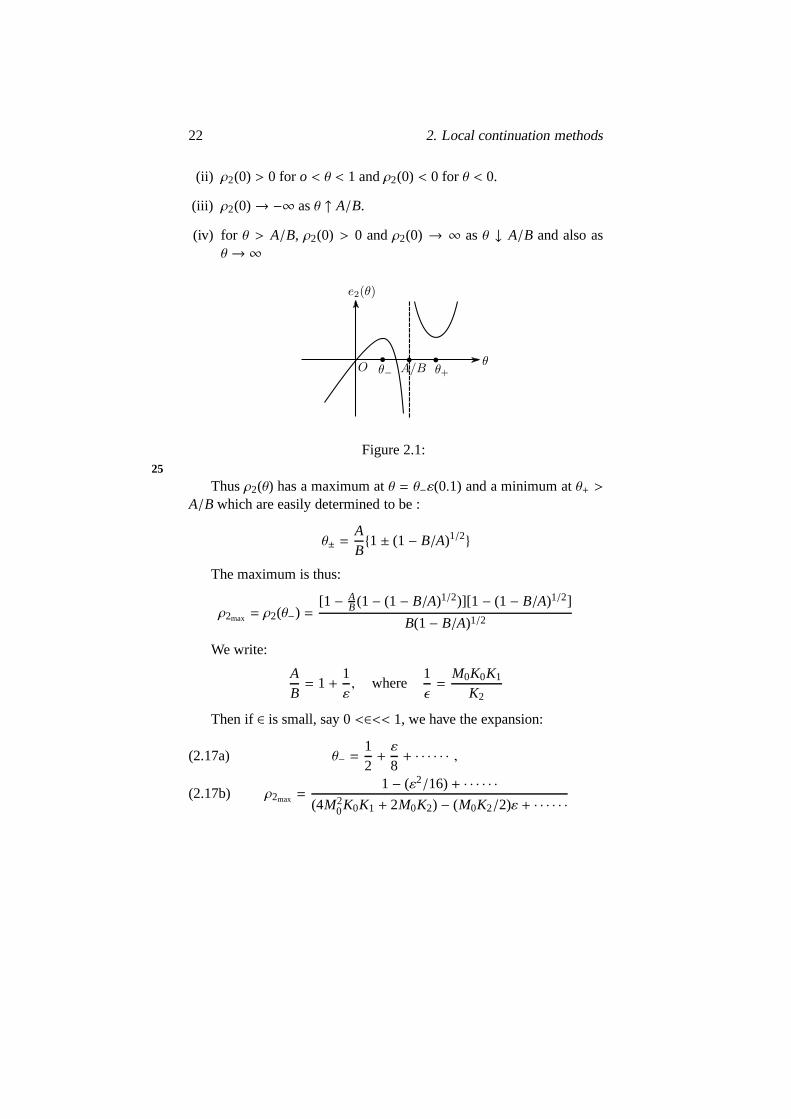
We want to maximizeρ2 as a function ofθ over (0, 1). The followingproperties hold (see Fig. 2.1):

(i) ρ2(0) = ρ2(1) = 0.


(ii) ρ2(0) > 0 for o < θ < 1 andρ2(0) < 0 for θ < 0.

(iii) ρ2(0)→ −∞ asθ ↑ A/B.

(iv) for θ > A/B, ρ2(0) > 0 andρ2(0) → ∞ asθ ↓ A/B and also asθ →∞

Figure 2.1:25

Thusρ2(θ) has a maximum atθ = θ−ε(0.1) and a minimum atθ+ >A/B which are easily determined to be :

θ± =AB1± (1− B/A)1/2

The maximum is thus:

ρ2max = ρ2(θ−) =[1 − A

B(1− (1− B/A)1/2)][1 − (1− B/A)1/2]

B(1− B/A)1/2

We write:

AB= 1+

1ε, where

1ǫ=

M0K0K1

K2

Then if∈ is small, say 0<∈<< 1, we have the expansion:

θ− =12+ε

8+ · · · · · · ,(2.17a)

ρ2max =1− (ε2/16)+ · · · · · ·

(4M20K0K1 + 2M0K2) − (M0K2/2)ε + · · · · · ·

(2.17b)

2.18. Approximate Implicit Function Theorem 23

We recall thatM0 = ‖(G0u)−1‖. Then ifG0

u becomes singular during26

continuation,M0 becomes infinite and the continuation procedure ex-plained here must fail. We notice this phenomenon first by therequiredstep sizes getting smaller. Also note that small steps result from largerK0, K1 andK2 as well.

In the implicit function theorem, we assumed that there is a solution(u0, λ0). Next we prove a similar theorem in which we assume only that‖G(u0, λ0)‖ is small.

2.18 Approximate Implicit Function Theorem

Let G : B1 × B2→ B1 satisfy for someδ > 0, ρ1 > 0, ρ2 > 0 sufficientlysmall:

(2.18)

(a) ‖G(u0, λ0)‖ ≤ δ for some u0 ∈ B1, λ0 ∈ B2.

(b) G0u is invertible and‖(G0

u)‖ ≤ M0

for some constantM0.

(c) G and Gu are continuous onBρ1(u0)×Bρ2(λ

0).

Then there exist u(λ), for all λ ∈ Bρ1(u0), such that:

(d) G(u(λ), λ) = 0 and u(λ) ∈ (U0)Bρ1(u0) [Existence].

(e) For a givenλ ∈ Bρ2(λ0) there is no solution of

G(u, λ) = 0 in Bρ1(u0) other thanu(λ) [uniqueness].

(f) u(λ) is continuous onBρ2(λ0) and has the same modulus

of continuity asGu(u, λ) [continuity].

Proof. We can prove the result in the same way as we have provedthe implicit function theorem. SinceG0

u is nonsingular, the problemG(u, λ) = 0 reduces to the fixed point problem

u = F(u, λ).

where 27

F(u, λ) = (G0u)−1[G0

uu−G(u, λ)].

New forλ ∈ Bρ2(λ0), we have:

‖u0 − F(u0, λ)‖ ≤ ‖u0 − F(u0, λ0)‖ + ‖F(u0, λ0) − F(u0, λ)‖,


and so:

(2.19a) ‖u0 − F(u0, λ)‖ ≤ M0(δ + ω0(ρ2)).

Hereω0 is given by (2.10)(2.10). Next, foru, v ∈ Bρ1(u0):

F(u, λ) − F(v, λ) = (G0u)−1[G0

u − Gu(u, v, λ)](u − v),

whereGu(u, v, λ) is defined as in (2.11a). Again using (2.11b,c,d) weobtain:

(2.19b) ‖F(u, λ) − F(v, λ)‖ ≤ M0(ω1(ρ1) + ω2(ρ2))‖u− v‖.

Now for anyθ ∈ (0, 1) , chooseρ1 andρ2, small enough, such that :

(2.19c) M0(ω1(ρ1) + (ω2(ρ2)) ≤ θ < 1,

and

(2.19d) M0(δ + ω0(ρ2)) ≤ (1− θ)ρ1.

Now we can apply the contraction mapping theorem to obtain theresults

2.20 Step Length Bound

We can also obtain step length bounds as before. Thus we assume (2.15)to hold and use it in (2.19d) to get

M0(δ + K0ρ2) ≤ (1− θ)ρ1

28

If we take :

(2.21a) ρ2 =(1− θ)ρ1 − M0δ

M0K0

then (2.19d) holds. Again from (2.19c), using (2.15) we require:

(2.21b) M0(K1ρ1 + K2ρ2) = θ < 1.

2.20. Step Length Bound 25

Substituting the value ofρ1 from (2.21a,b) we get:

ρ2(θ) =(1− θ)θ −C

A− Bθ,

where,A = M2

0K0K1 + B = M0K2,C = M20K1δ.

ρ2(θ) is sketched in fig. 2.2. We see thatρ2(θ) has a maximum atθ− ∈(0, 1) and a minimum atθ+ > A/B which are given by :

θ± =AB1± (1− B/A− (B2/A2)C)1/2.

The maximum is thus:

ρ2 max= ρ2(θ−).

We haveC > 0 andA − Bθ ≥ 0 if θ ≤ A/B. Henceρ2 max in thistheorem is less than that in the original implicit function theorem. Wewrite:

AB= 1+

1ε, where ε =

K2

M0K0K1,

and

C = M20K1δ = D · 1

ε,

whereD =M0K0δ

K0. If ε is small say, 0< ε << 1, then we have the29

expansions:

θ− =12

(1+ D) +ε

8(1− D)2

+ · · · · · · ,

and

ρ2 max=(1− D)2

+D2 (1− D)2ε − 1

8(1− D)4ε2+ · · · · · ·

(4M20K0K1 + 2M0K2 − 2M0K2D) − M0K2

2 (1− D)2ε + · · · · · ·

Again as before, we can see thatρ2 max is small if M0 is large. Notethat ρ2 max is always less thanρ2 max in the implicit function theorem.


Figure 2.2:

2.22 Other Local Rootfinders

Let g : R→ R be a smooth function. We will examine various methodsfor finding the roots ofg(x) = 0. In particular, we consider the chordmethod, Newton’s method etc. In the chord method, we choose an ini-tial estimatex0 of the solution and a slope a. Then the line with slope‘a’ through (x0, g(x0)) will intersect thex-axis atx1. This is the next ap-proximation to the solution. We continue the process withx1 replacing30

x0, using the same slope ‘a’ (See Fig. 2.3). More precisely,

a(x1 − x0) = −g(x0)

and in general

a(xk+1 − xk) = −g(xk)

The sequencesxk thus generated, converges to a zerog(x) if,

maxx∈H

∣∣∣∣∣1−g′(x)

a

∣∣∣∣∣ < 1,

whereH is an interval containing both the initial value and a root oftheequation.

2.23. Newton-Kantorovich Theorem 27

Figure 2.3:

In the higher dimensional case, we generalize the above to get thesequenceuU, form:

A[uU+1 − uU ] = −G(uU),

whereG : Rn→ Rn andA is ann× n matrix. In particular if we use:

a = g′(x0) andA = Gu(u0),

we get the special Newton method. 31

In Newton’s method we vary the slope at each iterate and take :

aU = g′(xU)

AU = GU(uU).

The Newton-Kantorovich theorem gives conditions under which theNewton iterate converge.

2.23 Newton-Kantorovich Theorem

Let G : B → B (B is a Banach space)satisfy for some u0 ∈ B andρ−0 > 0:(2.23)

(a) Gu(u0) is nonsingular with‖(G0u)−1‖ ≤ β;

(b) ‖G−u1(u0)G(u0)‖ ≤ α;(c) ‖Gu(u) −Gu(v)‖ ≤ γ‖u− v‖, in for all u, v ∈ Bρ−0 (u0) \ (u0)

(d) αβγ ≤12

and ρ−0 ≤1−

√1− 2αβγ

βγ.


Then the Newton iteratesuU defined by Newton’s method:

Gu(uU)[uU+1 − uU ] = −G(uU),U = 0, 1, 2, . . . . . .

with u0 = u0 satisfy:

(2.23)(e) uU ∈ Bρ−0 (u0).(f) uU converges tou∗, a root of G(u) =

0 in Bρ+0 (u0).

In addition u∗ is the is the unique root of G in Bρ+0 (u0) where32

ρ+0 = (1+ (1− 2αβγ)1/2)/βγ.

Proof. See the reference [16]

Now we prove a theorem, assuming the existence of a root, to showthe basic idea of how the above method works.

2.24 Newton Convergence Theorem

Let G : B→ B and G(u) = 0 have a root u= u∗. For someρ∗ > 0 let Gsatisfy:

(2.24)

(a) ‖G−1u (u∗)‖ ≤ β.

(b) ‖Gu(u) −Gu(v)‖ ≤ γ‖u− v‖, for all u, v ∈ Bρ∗(u∗).

(c) ρ∗βγ <23.

Then for every u0 ∈ Bρ∗(u∗) the Newton iterates satisfy:

(2.24)(d) uU ∈ Bρ∗(u

∗);(e) ‖uU+1 − u∗‖ ≤ a‖uU − u∗‖2;

where,

a ≡Bγ

2(1− ρ∗βγ)<

1ρ∗.

2.24. Newton Convergence Theorem 29

Proof. For anyu ∈ Bρ∗(u∗) we have the identity :

Gu(u) = Gu(u∗)I +G−1u (u∗)[Gu(u) −Gu(u∗)].

Then (2.24a,b,c) imply that:

‖G−1u (u∗)[Gu(u) −Gu(u∗)]‖ ≤ ρ∗βγ <

23.

Hence, by the Banach lemma,I +G−1u (u∗)[Gu(u) −Gu(u∗)] is in- 33

vertible and so isGu(u). From the same lemma we get the estimate :

(2.25) ‖G−1u (u)‖ ≤

β

1− ρ∗βγ.

Now we will prove by induction thatuU ∈ Bρ∗(u∗), u = 0, 1, 2, . . ..

SupposeuU ∈ Bρ∗(u∗). Then

uU+1 − u∗ = (uU − u∗) −G−1u (uU )[G(uU) −G(u∗)].

By the mean value result (2.6), we have :

G(uU) −G(u∗) = Gu(uU , u∗)(uU − u∗),

and so:

uU+1 − u∗ = G−1u (uU)[Gu(uU) − Gu(uU , u

∗)](uU − u∗).

But

‖Gu(uU) − Gu(uU , u∗)‖ ≤

1∫

0

‖Gu(uU ) −Gu(tuU + (1− t)u∗)‖dt

≤ γ1∫

0

‖(1− t)(uU − u∗)‖dt

=γ

2‖uU − u∗‖.


Hence

‖uU+1 − u∗‖ ≤ ‖G−1u (uU)‖.γ

2‖uU − u∗‖2,

≤β

1− ρ∗βγγ

2‖uU − u∗‖2,

(2.26)

by (2.25). Note that

βγ

2(1− ρ∗βγ)≤

1ρ∗

and‖uU − u∗‖ ≤ ρ∗.

HenceuU+1 ∈ Bρ∗(u∗) and by induction (d) follows. Then (e) fol-34

lows from (2.26).

Note.The convergence here, is quadratic. Thus if

a‖uU − u∗‖ ≤ 10−pU

for some positivepU , then

a‖uU+r − u∗‖ ≤ 10−2uρU ‖uU − u∗‖ for anyr = 0, 1, 2, . . . . . . .

The choice of the initial iterate,u0, is important in using Newton’smethod. It is not uncommon to spend 90% or more of the effort infinding a food approximate value of the root. Our study will show manyways in which such difficulties can be overcome. Another problem withNewton’s method can be the time it takes to solve the linear system forthe new iterate. This occurs, for example, ifB = RN for very largeN,sayN ≈ 103 or larger (when approximating nonlinear P.D.E. problems).The so calledquasi-Newton methodsare designed to avoid the linearsystem problem by some device (for example updating secant method,which we are going to describe in the next section).

2.27 Predictor-Solver Methods

Let G : RN × R → RN. At the root (u0, λ0) of G(u, λ) = 0, let G0u be

nonsingular. Then the implicit function theorem shows the existence of

2.27. Predictor-Solver Methods 31

the unique branch of solutionsu = u(λ) in a neighbourhood ofλ0. Wewill briefly describe variouspredictor-sovler methodsfor determiningu(λ). These proceed by using the solution (u0, λ). to construct a betterapproximationu0(λ) to the actual solutionu(λ). This is the predictor.After obtaining the initial approximation, we apply an iteration scheme 35

for which the sequence of iterates converges to the solutionu(λ). Thisis the solver.

Various Predictors

(i) Trivial Predictor : Here we take the initial approximation as (see(Fig. 2.4a)):

u0(λ) = u0= u(λ0)

i.e. the initial guess atλ is equal to the solution atλ0. The errorestimate is given by :

||u(λ) − u0(λ)|| = ||u(λ) − u(λ0)||,

≤M0

1− θω0(|λ − λ0|).

Hereu(λ) is the actual solution andω0 is given by (2.10). IfG(u, λ)is Lipshitz continuous inu then

||u(λ) − u0(λ)|| ≤m0

1− θK0|λ − λ0|,

whereK0 is the corresponding Lipshitz constant.

(ii) Secant-Predictor: Here we assume that there are two known solu-tions (u0, λ0) and (u1, λ1). Then consider the line segment joining(u0, λ0) and (u1, λ1) in the (u, λ) space. Takeu0(λ) as the point onthis line with givenλ-coordinate valueλ. (See Fig. 2.4b) i.e.

u0(λ) = u1+ (λ − λ1)

u1 − u0

λ1 − λ0.

Then 36


u(λ) − u0(λ) = [u(λ) − u(λ1)] − λ − λ1

λ1 − λ0[u(λ1) − u(λ0)],

= uλ(λ, λ1)(λ − λ1) − (λ − λ1)uλ(λ

1, λ0).

By the mean value formula (2.6):

u(λ) − u0(λ) =

1∫

0

dt[uλ + (1− t)λ1) − uλ(tλ1+ (1− t)λ0)](λ − λ1),

=

1∫

0

dt

1∫

0

uλλ(s(tλ + (1− t)λ1) + (1− s)(tλ1+ (1− t)λ0))

(t(λ − λ1) + (1− t)(λ1 − λ0))(λ − λ1)ds.

Again we have use (2.6). Thus we get:

||u(λ) − u0(λ)|| ≤12

K2[(λ − λ1) + (λ1 − λ0)](λ − λ1),

=12

K2(λ − λ0)(λ − λ1), λ0 < λ1 < λ,

where,

K2 = K2(λ) ≡ maxλ∈[λ0,λ]

||uλλ(λ)||.

Sinceλ0 < λ1 < λ, this is an extrapolation.

In the interpolation case, that is ,λ0 < λ < λ1, we have :

||u(λ) − u0(λ)|| ≤ 12

K2(λ − λ0)(λ1 − λ).

2.27. Predictor-Solver Methods 33

(a) (b)

Figure 2.4:

(iii) Higher-order Predictor (Lagrange): If we know more than two 37

solutions, then we can take higher order approximations to the nextsolution by using order interpolation formulae.

(iv) Tangent Predictor (Euler method): In the secant predictor meth-od we assumed the existence of two solutions and then used theline segment joining these two solutions. Now we will consideronly the solution at a single point and use the tangent to the solu-tion curve at that point. (see Fig. 2.4). From the implicit functiontheorem we have:

G(u(λ), λ) = 0 for all λ ∈ Bρ2(λ0).

Differentiating with respect toλ, we get:

Gu(u(λ), λ)u(λ) = −Gλ(u(λ), (λ),

and thusu0= u(λ0) = −(G0

u)−1G0λ.

Then we take the approximation as :

u0(λ) = u0+ (λ − λ0)u0.

The error is given by:

u(λ) − u0(λ) =12

u0(λ − λ0)2+ 0((λ − λ0)3).


Figure 2.4: (c)

Solvers: Now using predictoru0(λ), our aim is to construct an iteration38

scheme of the form

AU(uU+1 − uU) = −G(uU , λ),U = 0, 1, 2, · · · · · · ,

whereAU are suitable matrices which assure the convergence ofuU to a root

(i) Special Newton Method

In the special special Newton method,AU is given by the constantoperatorG0

u.

(ii) Newton’s Method

In Newton’s method,AU ≡ GUu = Gu(uU , λ). One of the impor-

tant advantages of Newton’s method is that it can have quadraticconvergence i.e. the sequence (uU) satisfies :

||uU+1 − u∗|| ≤ β||uU − u∗||2,

for some constantβ, whereu∗ is the actual solution.

(iii) Updating-Secant Method

As mentioned above a major disadvantage of Newton’s method isthat we need to solve a linear system with the coefficient matrixGU

u stepU = 0, 1, 2, . . . . . .. This costs 0(N3) operations at eachstep, whereN is the dimension of the space.

2.29. Lemma 35

Now we will introduceUpdating-Secant Method.The idea of thisiteration scheme is to obtain a suitable approximationAU to GU

u so that39

the system at (U + 1)st stage can easily be solved if we can solve thesystem atU th stage. FurtherAU+1 is to satisfy a relation also satisfiedby GU+1

u . We will takeAU+1 in the form:

(2.28) AU+1 = AU +CURTU ,

whereCU andRU are column vectors of dimensionN andAU is anN×Nmatrix. In particular we choose:

CU ≡(yU − AUSU)< SU ,SU >

,

andRT

U ≡ STU ,

whereyU = G(xU+1) −G(xU) andSU = xU+1 − xU .

Now we have to solve the linear systemAUSU = −G(xU) at eachstep. But this can be easily achieved using the Shermann-Morrison for-mula [for more details see [12]).

2.29 Lemma

Let A be anN × N invertible matrix andu, v ∈ RN. ThenA + uvT isnonsingular if and only ifσ = 1+ (v,A−1u) , 0, and then the inverse of(A+ uvT ) is given by

(2.29a) (A+ uvT )−1= A−1 −

1σ

A−1uvTA−1

Using this result and (2.27), the inverse ofAU+1 is given by

(2.29b) A−1U+1 = A−1

U +(sU − A−1

U yU)sTU A−1

U

(sU ,A−1U yu)

40


This method uses only 0(N2) arithmetic operations. Naturally, wecan expect a loss in the rate of convergence compared to Newton’smethod here we get onlysuperlinear convergenceinstead of quadraticconvergence. i.e.

||uU+1 − u∗|| ≤ αU ||uU − u∗||

whereαU → 0 asU → ∞

This is generally known as a Quasi-Newton method (see ref: [9]).

Chapter 3

Global continuation theory

3.1 Introduction41

In this section we will discuss some preliminary aspects which are use-ful in the study ofglobal continuation results. We will start with somedefinitions regarding the functionG from RM into RN. The Jacobian ofG(x) is:

G′(x) =∂G∂x

(x) = (gi

x j(x1, . . . , xM))1≤ j≤M

1≤i≤N,

wherex = (x1, . . . xM)T andG = (g1, . . . gN)T ·G′(x) is anN×M matrixand its rank must be less than or equal ti min (N,M).

Definitions. (1) LetG be continuously differentiable. Let

C = x ∈ RM : RankG′(x) < min(N,M).

The points inC are called critical points ofG.

(2) The regular points are the points in the complement ofC, denotedby RM \C.

Note: The domainRM can always be replace by the closure of anopen set inRM.

(3) The image of the setC underG, i.e. G(C) which is a subset ofRN 42

is the set of critical values ofG.

37

38 3. Global continuation theory

(4) The complement ofG(C) in RN is the set of regular values ofG.i.e. RN \G(C).

Now we will state and proveSard’s Theorem(See [26]).

3.2 Sard’s Theorem

Let G∈ C1(RM) ∩CM−N+1(RM). Then G(C) hasRN - measure zero.

Proof. We will prove the result forM = N. The caseM < N is trivial.In this case there exist a nontrivial null vector ofG′. This is preciselythe idea we are going to use in the caseM = N. For M > N see [1].

So assumeM = N. Let Q0 be an arbitrary cube inRN of side L.(Therefore vol (Q0) = LN). We will show that volume (G(C ∩ Q0)) iszero which implies that the measure ofG(C) is zero, sinceL is arbitrary.

With ℓ = Ln , let q j be the set cubes of sideℓ, for j = 1, 2, . . . nN,

which form a partition ofQ0. i.e.

Q0 =

nN⋃

j=1

q j .

Assume that eachq j contains at least one critical point, sayx j. Letx ∈ q j , then

G(x) = G(x j+ (x− x j))

= G(x j) +G′(x j)(x− x j) + o(ℓ),

whereo(ℓ)ℓ→ 0 asℓ→ 0.

Using the fact that, rankG′(x j) ≤ N − 1, we will show that for43

sufficiently smallℓ, zj(x) = G′(x j)(x − x j) lies in N − 1 dimensionalsubspace ofRN as x varies. To see this, letξ j be a unit null vector ofG′(x j). Put

y j(x) = x− x j= [y j− < y j , ξ j > ξ j]+ < y j , ξ j > ξ j .

3.3. Examples 39

Note that the vectory j− < y j, ξ j > ξ j has no component in theξ j

direction and hence it lies in anN−1 dimensional subspace ofRN. As xvaries overq j , all these vectorszj(x) lie in the sameN−1 dimensionalsubspace. SinceG′(x j) is independent ofx, the measure of the set

G′(x j)y j(x) : x ∈ q j

is less than or equal to (Kℓ)N−1, whereK is a constant (maximum elon-gation constant forG on Q0). Hence the volume ofG′(x j)y j(x) + o(ℓ) :x ∈ q j is less than or equal to (Kℓ)N−1 × o(ℓ). Thus

VolG(C ∩ Q0) ≤ nN(Cℓ)N−1o(ℓ)

= (CN−1LN)o(ℓ)ℓ→ 0 asℓ → 0.

This proves Sard’s theorem for the caseM ≤ N.

3.3 Examples

(1) Consider the example from population dynamics:

G(u, λ) = u2 − λ1u− λ2.

Take

x ≡

x1

x2

x3

=

uλ2

λ3

.

ThenG(u, λ) and its derivative can be written as 44

G(x) = x21 − x2x1 − x3,

G′(x) = [2x1 − x2,−x1,−1].

Rank (G′(x)) = 1, which is the maximum rank. Therefore thereare no critical points for this problem.

(2) DefineG : R2→ R by:

G(x) = x21 − x2x1 − k wherek is a constant.


ThenG′(x) = [2x1 − x2,−x1].

and it has the maximum rank 1, except atx = (0, 0) whereG′(x) hasrank zero. This is a critical point and it is the only criticalpoint. Thecritical value isG(0) = −k.

Observe that the solution curves ofG(u) = 0 are two disjoint curvesfor k , 0. Fork = 0 they are two lines which intersect at the origin,which is a bifurcation point. See Fig. 3.1.

Figure 3.1:

3.4 Solution sets for Regular Values45

We study now the solutions ofG(x) = p, Wherep is a regular value.

3.5 Lemma (Finite Set of Solutions)

Let G : RN → RN with G ∈ C1(Ω), for some bounded open setΩ ⊂ RN.Let p∈ RN be a regular value of G such that:

G(x) , p for x ∈ ∂Ω.

Then the set G−1(p) ∩ Ω is finite, where:

G−1(p) = x ∈ RN : G(x) = p.

3.6. Lemma (Global Solution Paths) 41

Proof. We give a proof by contradiction. Letx j∞j=1 ∈ G−1(p) ∩ Ω andassume allx j ’s are distinct. Then some subsequence ofx j convergesto somex∗ ∈ Ω. By the continuity ofG, we have:

G(x∗) = p.

This impliesx∗ < ∂Ω. However by the implicit function theorem,there is one and only one solutionx = x(p) of G(x) = p in some openneighbourhood ofx(p). This is a contradiction, since every neighbour-hood ofx∗ contains infinitely mayx j ’s. This complete the proof.

Next, we will consider the caseG : RN+1 → RN and study thesolution setG−1(p), if p is a regular value.

3.6 Lemma (Global Solution Paths)

Let G : RN+1 → RN, and G ∈ C2(RN+1). Let p be a regular value 46

for G. Then G−1(p) is a C1, one dimensional manifold. That is each ofits connected components is diffeomorphic to a circle or infinite inter-val. In more detail, each component of G−1(p) can be represented by adifferentiable function X(s), s∈ R and it satisfies one of the following:

(3.6)(a) ||X(s)|| → ∞ as|s| → ∞.(b) X(s) is a simple closed curve andX(s) is periodic.(c) G−1(p) = φ.

Proof. Assume thatG−1(p) , φ, or else we are done. Letx0 be suchthat:

G(x0) − p = 0.

Consider the equation:

G(x) − p = 0.

Sincep is regular value, the Jacobin ofG(x) − p at x0 viz. G′(x0),must have the maximum rankN. Therefore, it has a minor of orderN,


which is nonsingular. Assume that∂G

∂(x1, , , xN)(x0) is nonsingular. Let

(xi , ..xN) = u andxN+1 = λ. Thus we have:

F(u0, λ0) ≡ G(u0, λ0) − p = 0,

andFu(u0, λ0) = Gu(u0, λ0)

is nonsingular. Hence by the implicit function theorem there exists aunique solutionu = u(λ), for all λ such that|λ − λ0| < p1(u0, λ0). i.e.there exits a solution are:47

γ1= x1(xN+1), . . . , xN(xN+1), xN+1,

with XN+1 in some iterval|xN+1 − x0N+1| < ρ1(x0). Extend this arc over

a maximal interval (the interval beyond which we cannot extend thesolution), say,xL

N+1 < xN+1 < xRN+1.

At the points, the Jacobian∂G

∂(x1, ..xN)(x0) will be singular, other-

wise we can again apply implicit function theorem to obtain the solutionin a larger interval which will contradict the maximality ofthe interval.Now consider the pointxR

= (x1(xRN+1), . . . (xN(xR

N+1), xRN+1). By the

continuity ofG we have:G(xR) = p.

Again sincep is a regular value, there exists a minor of rankN,which is nonsingular. Assume that this is obtained from the matrix Gx

by removing thejth column of the matrix. As before, there exists an areγ2, say,

γ2= x1(x j), . . . x j−1(x j), x j , x j+1(x j), . . . xN+1(x j),

over a maximal interval. We can continue this procedure indefinitely.This family (γi) will overlap because the implicit function theorem gives

3.7. Degree Theory 43

a unique curve. Thusγi form aC1 curve. This curve can be globallyparametrized. Suppose it is given by:

Γ = X(s); X(sa) = x0, sa ≤ s≤ sb

and 48

G(X(s)) = p.

If X(s) is not bounded, then the first part of the theorem follows. Soassume thatX(s) is bounded. Then choose a sequencesj → ∞ suchthatX(sj) → x∗. By the continuity ofG we get:

G(x∗) = p.

If the curve is not closed,x∗ will be a limit point and also a solutionof G(x) − p = 0. Sincep is a regular value, we can apply the implicitfunction theorem to conclude that the curve has to be closed.This closedcurve is simple, because of the uniqueness of the solution path. Hencein the case whenX(s) is bounded, we have a simple closed periodicsolution which proves part (b) of the theorem.

Remark . The main idea in the proof is the change of parameter fromone componentγ j to another. This can be used as a practical procedurefor carrying out global continuation; see [27].

3.7 Degree Theory

In this section we will assign an integer, called the ‘degree’ to a continu-ous functionF, defined on an open subsetΩ, of RN and a pointp ∈ RN.This is an important tool in proving fixed point theorems and existenceresults for nonlinear problems. The degree of a continuous functionFover a domain at a pointp has the important property that if it is non -zero, then there exists a solution ofF(x) = p in the given domain. An- 49

other important property is that it depends on the values of the functiononly on the boundary and not in the interior.


3.8 Definition

Let F : RN → RN andp ∈ RN satisfy:

(i) F ∈ C1(Ω), whereΩ is an open bounded subset ofRN,

(ii) p < F(∂Ω),

(iii) p is a regular value ofF onΩ.

Then the degree ofF onΩ for p is defined as:

(3.8) deg(F,Ω, p) =∑

x∈[F−1(p)∩Ω]

Sgn[detF′(x)].

Note.The degree is well defined, since by lemma 3.5, [F−1(p)∩ Ω] is afinite set and hence the right hand side is a finite sum.

Example.Considerf : R → R such thatf ′(x) is continuous on [a, b]and f (a) , p, f (b) , p and f (x) = p has only simple roots on [a, b].Then

deg(f , (a, b), p) =k∑

j=1

f ′(x j)

| f ′(x j)|,

wherex jkj=1 are the consecutive roots off (x) − p = 0 contained in[a, b]. In this particular case, iff ′(x j) > 0, then f ′(x j+1) < 0 and vice

versa. Thereforef ′(x j)

| f ′(x j)|= +1 and−1 alternatively. Hence

deg(f , (a, b), p) ∈ 1, 0,−1.

Now if p does not lie betweenf (a) and f (b), then there are eitherno roots or an even number of roots for the equationf (x) = p in (a, b).50

Hence the degree is zero. In the other case, there will be an odd numberof roots, say (2k+1), k ≥ 0. Thus in the summation in (3.8), the first (2k)terms cancel out and the last term is+1 or−1, depending onf (b) > por f (b) < p. Hence we can write:

deg(f , (a, b), p) =12

[f (b) − p| f (b) − p|

−f (a) − p| f (a) − p|

].

3.9. Definition 45

Note that in this case the degree depends only on the values off atthe boundary pointsa andb. This is true in the general case also.

Next we will relax condition (iii) of definition 3.8.

3.9 Definition

Let F satisfy (i) and (ii) of (3.8). Then,

(3.9a) deg(F,Ω, p) ≡ deg(F,Ω, q),

whereq satisfies:

(3.9b)(i) q is a regular value ofF,

(ii) ||q− p|| < γ ≡ dist (F(∂Ω), p) ≡ inf x∈∂Ω ||F(x) − p||.

By Sard’s theorem, the set of all regular values ofF are dense inR

N. Hence we can find regular values satisfying (3.9b(ii)). Also if q1,q2 are two regular values satisfying (3.9b(ii)), then they belong to thesame connected component ofRN \ F(∂Ω) and hence (for a proof whichis too lengthy to include here see [29]):

deg(F,Ω, q1) = deg(F,Ω, q2).

Therefore the above degree is well defined. We can also relax con-dition (i) of definition 3.8 and define the degree forF ∈ C(Ω). 51

3.10 Definition

AssumeF satisfies:

(i) F ∈ C(Ω).

(ii) p < F(∂Ω).

Then

(3.10) deg(F,Ω, p) ≡ deg(F,Ω, p)

whereF satisfies, usingy of (3.9b(ii)):


(iii) F ∈ C1(Ω),

(iv) ||F − F ||∞ <γ

2.

SinceF is continuous, we can approximateF as closely as desired,by differentiable functionF. (Take polynomials, for example). Con-ditions (ii) and (iv) imply thatp 6 εF(∂Ω). Thus deg (F,Ω, p) is welldefined by definition 3.9. IfF is another smooth function, satisfyingcondition (iv), then by considering the homotopy

G(x, t) = tF(x) + (1− t)F(x)

and using the homotopy invariance property of the degree in definition3.8 (which we prove next), it follows that

deg(F,Ω, p) = deg(F,Ω, p).

Thus definition 3.10 is independent of the choice ofF. Thus thedegree is well defined even for a functionF ∈ C(Ω).

3.11 Theorem (Homotopy Invariance of the Degree)52

Let G : RN+1→ RN,Ω bounded open set inRN and p∈ RN satisfy:

(3.11)

(a) G ∈ C2(Ω × [0, 1]),(b) G(u, λ) , p on∂Ω × [0, 1],(c) G(u, 0) ≡ F0(u), G(u, 1) ≡ F1(u),(d) p is a regular value forG onΩ × [0, 1] and for F0 andF1 on Ω.

Thendeg(G(., λ),Ω, p) is independent ofλ ∈ [0, 1]. In particular,

deg(F0,Ω, p) = deg(F1,Ω, p).

Proof. The proof uses lemma 3.5. We will prove

deg(F0,Ω, p) = deg(F1,Ω, p).

3.11. Theorem (Homotopy Invariance of the Degree) 47

The case for anyλ ∈ (0, 1) is included. Sincep is a regular value,we have:

F−10 (p) ∩ Ω = u0

i ,

andF−1

0 (p) ∩ Ω = u1j ,

whereu0i and u1

j are finite sets by lemma 3.5. Again, sincep is a

regular value,G−1(p)∩(Ω×[0, 1]) is a finite collection of arcs, denotedby Γi(s). Let us parametrize anyΓ(s) as (u(s), λ(s)), wheres denotesthe arc length. OnΓ(s) we have:

G(s) ≡ G(u(s), λ(s)) = p.

Differentiating with respect tos, we get : 53

Gu(s) · u(s) +Gλ(s)λ(s) = 0.

Sinces is the arc length, we have:

uT (s)u(s) + λ(s)λ(s) = 1.

These two equations together can be written as:

(3.12a) A(s)

(u(s)

λ(S)

)=

(01

),

where

A(s) =

[Gu(s) Gλ(s)uT(s) λ(s).

]

We shall show thatA(s) is nonsingular onΓ(s). First observe thatat each point onΓ(s), there is a unique tangent to the path. The matrix[Gu(s),Gλ(s)] has rankN, sincep is a regular value. Thus the null spaceof this matrix is one dimensional. Let is be spanned by the vector ξ, n.Since (u, λ) is also a null vector, we have:

(u(s), λ(s)) = c1(ξ, η), for somec1 , 0.


Now if A(s) is singular, then it must have a nontrivial null vector ofthe formc2(ξ, η) for c2 , 0. Since

c2A(s)(ξ

η) = 0,

the last equation gives:

c1c2(|ξ∼|2 + η2) = 0.

This implies thatc1c2 = 0, a contradiction. HenceA(s) is nonsingu-54

lar.Now apply Cramer’s rule to solve the above system forλ(s) to get:

(3.12b) λ(s) =detGu(s)detA(s)

Note that onΓ(s), det A(s) , 0. The above result shows thatλ(s)and detGu(s) change sign simultaneously.

We have by (3.8)

deg(F0,Ω, p) =∑

u0i

sgn(detF′0(u0i )),

deg(F0,Ω, p) =∑

u1i

sgn(detF′1(u1i )).

Observe that the arcsΓ(s) can be classified into four different types:

(i) arcs joining two points fromu0i

(ii) arcs joining two points fromu′j

(iii) arcs joining a pointu0i to a pointu1

j

(iv) arcs with no end points.

3.11. Theorem (Homotopy Invariance of the Degree) 49

We shall use the arcs of type (i), (ii) and (iii) to relate the above twodegrees.

Figure 3.2:

In case (i),λ(s) has different signs at the end points, since along55

the Γ(s), λ(s) changes sign an odd number of times. Hence detGu(s)has different signs at the end points. Therefore no contribution to deg(F0,Ω, p) results from points. Similar result is true for case (ii). Ob-viously there is no contribution to the degree from the (iv)th case. Sothe only contribution comes from case (iii). Here note thatλ(s) andhence detGu(s) have the same sign at both the end points, becauseλ(s)changes sign an even number of times. This shows that:

deg(F0,Ω, p) = deg(F1,Ω, p)

The theorem is true for the other two definitions of degree also. In-deed when these definitions have been justified, our above proof givesthe desired result with the hypothesis relaxed to continuous mappingsand without the restriction (3.11d).

Some Important Properties of the Degree

(1) f , g : Ω→ RN be such that:


(i) f (x) = g(x) for all x ∈ ∂Ω;

(ii) f (x), g(x) ∈ C(Ω);

(iii) f (x) , p for all x ∈ ∂Ω;

Then

deg(f ,Ω, p) = deg(g,Ω, p).

(2) If p, q are close to each other, say,

||p− q|| < γ = dist (f (∂Ω), p).

Then56

deg(f0,Ω, p) = deg(f1,Ω, q).

(3) Let f , g : Ω→ RN be continuous andp < f (∂Ω)Ug(∂Ω). Let f andg satisfy

supx∈∂Ω| f (x) − g(x)| <

γ

2.

Then

deg(f ,Ω, p) = deg(g,Ω, p).

(4) Homotopy invariance property.

(5) (Excision) IfK is a closed set contained inΩ andp < f (K)U f (∂Ω),then

deg(f ,Ω, p) = deg(f ,Ω\K, p).

(6) Let p < f (Ω), then

deg(f ,Ω, p) = 0.

(7) If deg(f ,Ω, p) , 0, then f (x) = p has a solution inΩ. (For refer-ence, See : [26], [29])

3.13. Brouwer Fixed Point Theorem 51

Application 1. Fixed points and roots

3.13 Brouwer Fixed Point Theorem

Let F : RN → RN satisfy:

(3.13)(a) F ∈ C(Ω),Ω is a convex open bounded subset ofRN.

(b) F(Ω) ⊂ Ω.Then F(u) = u for some u∈ Ω. 57

Proof. Take any pointa ∈ Ω. Define

G(u, λ) = λ(u− F(u)) + (1− λ)(u− a).

We shall thatG, a homotopy between (u − F(u)) and (u − a), doesnot vanish on∂Ω × [0, 1].

If G(u, λ) = 0, then we have :

u = λF(u) + (1− λ)a

By (3.13b) we get,F(u) ∈ Ω. Sincea ∈ Ω, by convexityu ∈ Ω forλ ∈ [0, 1]. ThereforeG(u, λ) , 0 on∂Ω×[0, 1]. So homotopy invariancetheorem implies that:

deg(u− F(u),Ω, 0) = deg(u− a,Ω, 0)

= [sgndetI ]u=a

= 1

Henceu− F(u) = 0 has a solution inΩ

Note. If F ∈ C2(Ω) the above proof is constructive. That is we can findarbitrarily good approximations to the fixed point by computation. Todo this we consider:

G(u, λ) = λ(u− F(u)) + (1− λ)(u− a) = 0

and follow the pathΓ(s) from (u(0), λ(0)) = (a, 0), to (u(sF), λ(sF)) =(F(u(sF)), 1). If 0 is not a regular value, we can takeδ arbitrarily smalland a regular value. Then we can construct solutions foru − F(u) = δ.It can be shown that 0 is a regular value for almost alla ∈ Ω. 58

Another result on global existence of a solution is given as:


3.14 Theorem

Let F ∈ C(Ω), whereΩ is open inRN and satisfy, for some x0 ∈ Ω:

(3.14) < x− x0, F(x) >> 0 for all x ∈ ∂Ω.

Then F(x) = 0 for some xεΩ.

Proof. Consider the homotopy

G(x, λ) = λ f (x) + (1− λ)(x− x0), 0 ≤ λ ≤ 1.

It is easy to prove thatG(x, λ) , 0 on∂Ω and for all 0≤ λ ≤ 1. Forif not, taking the inner product with (x− x0), we get:

< x− x0, F(x) > +(1− λ)||x− x0||2 = 0.

If x ∈ ∂Ω then this gives a contradiction by (3.14). HenceG(x, λ) , 0for x ∈ ∂Ω and 0≤ λ ≤ 1. Therefore

deg(F,Ω, 0) = deg(x− x0,Ω, 0) = 1

Application II. Periodic solutions of O.D.E.

We shall use the Brouwer theorem to show the existence of periodicsolutions of systems of ordinary differential equations.

3.15 Periodic Solution Theorem59

Let f(t, y) : R×RN → RN satisfy for some T> 0 and some convex openΩ ⊂ Rn.

(3.15)

(a) f ∈ C([0,T] × Ω).(b) f (t + T, y) = f (t, y) for all y ∈ Ω(c) || f (t, y) − f (t, x)|| ≤ K||x− y|| for all

x, y ∈ Ω, 0 ≤ t ≤ T,K > 0.(d) f (t, y) is directed intoΩ for all

y ∈ ∂Ω andt∈[0,T],

3.15. Periodic Solution Theorem 53

i.e. for all y∈ ∂Ω, y+ ε f (t, y) ∈ Ω, for all ε > 0 sufficiently small. Thenthe equation

(3.15e)dydt= f (t, y)

has periodic solutions y(t) with period T and y(t) ∈ Ω, for all t.

Proof. Pick anyu ∈ Ω and solve the initial value problem :

dydt= f (t, y),

y(0) = u.

Let the unique solution in the interval [0,T] be denoted byy(t, u).Theny(t, u) ∈ Ω for all t > 0. Otherwise, lett1 be the first time it crossesthe boundary ofΩ. That isy(t1, u) ∈ ∂Ω, t1 > 0, y(t, u) ∈ Ω, for all0 ≤ t < t1 and,

y(t1, u) = f (t1, y).

But condition (3.15d) says thatf (t1, y) is directed intoΩ which isnot possible. Now considerF(u) ≡ y)(T, u), for uεΩ; this F satisfies allthe hypothesis of the Brouwer fixed point Theorem. Hence we have:

y(T, u) = u, for someuεΩ.

i.e. we have a periodic solution passing throughu. 60

Application III. Bifurcation by degree theory

Definition. Let G : RN × R→ RN beC1. Consider the problem:

(3.16) G(u, λ) = 0.

Given a smooth path (or arc) of solutions, say,

Γ = (u(λ), λ) : λa < λ < λb,


a point (u0, λ0) ∈ Γ is said to be a bifurcation point for (3.16) if everyball Bρ(u0, λ0) ⊂ RN+1, of radiusρ > 0, contains solutions of (3.16) notonΓ.

The following theorem shows that if the sign of detGu(u(λ), λ)changes at some point alongΓ, then it is a bifurcation point. This isan important result in testing for bifurcation.

3.17 Theorem (Bifurcation Test)

Let Γ be a smooth solution arc of(3.16) parametrized byλ. Let detGu(u(λ), λ) change sign atλ0 ∈ (λa, λb). Then(u(λ0)λ0) is a bifurcationpoint of (3.16).

Proof. We prove by contradiction. Assume that,

(u0, λ0) = (u(λ0)λ0),

is not a bifurcation point. Hence there exists a ball of radius ρ, whichdoes not contain any root of (3.16) other on the arcΓ. Chooseη, δ > 061

small enough so that the cylinder:

Cη,δ = (u, λ) : u ∈ Kη(u0), λ ∈ [λ0 − δ, λ0

+ δ],

where,

Kη(u0) = u ∈ RN : ||u− u0|| ≤ η.

is such that :

(i) Cη,δ ⊂ Bρ(u0, λ0).

(ii) G(u, λ) , 0, for all (u, λ) ∈ ∂Kη × [λ0 − δ, λ0+ δ].

(iii) u(λ0 ± δ) ∈ Kη(u0).

(iv) det Gu(u(λ), λ) does not change sing in the intervals (λ0 − δ, λ0)and (λ0, λ0

+ δ).

3.17. Theorem (Bifurcation Test) 55

We can easily chooseη andδ so that (i) is satisfied. Since the ballBρ(u0, λ0) contains no roots other than on the areΓ and detGu(u(λ), λ)changes sing atλ0 and is continuous we can shrinkδ (if necessary) sothat (ii), (iii) and (iv) are satisfied (see Fig. 3.3).

Figure 3.3:

Applying the homotopy theorem to the functionG(., λ0 − δ) and 62

G(., λ0+ δ), we get:

deg(G(., λ0 − δ),Kη(u0), 0) = deg(G(., λ0

+ δ),Kη(u0), 0).

But

deg(G(., λ0 − δ),Kη(u0), 0) = Sgn degGu(u(λ0 − δ), λ0 − δ),

and

deg(G(., λ0+ δ),Kη(u

0), 0) = Sgn degGu(u(λ0+ δ), λ0

+ δ).

This is a contradiction, because detGu(u(λ), λ) has different signs at(u(λ0

+ δ), (λ0 − δ) and (u(λ0+ δ), λ0

+ δ).

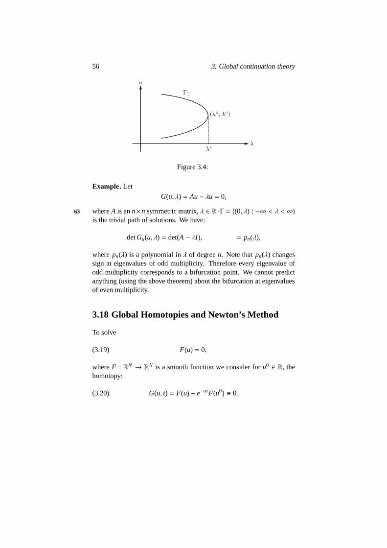
Note.Hereλ0 ∈ (λa, λb) is an interior point of the interval. We cannotapply this theorem ifλ0 is a boundary point. See Fig. 3.4.


Figure 3.4:

Example.Let

G(u, λ) = Au− λu = 0,

whereA is ann×n symmetric matrix,λ ∈ R ·Γ = (0, λ) : −∞ < λ < ∞63

is the trivial path of solutions. We have:

detGu(u, λ) = det(A− λI ), = pn(λ),

wherepn(λ) is a polynomial inλ of degreen. Note thatpn(λ) changessign at eigenvalues of odd multiplicity. Therefore every eigenvalue ofodd multiplicity corresponds to a bifurcation point. We cannot predictanything (using the above theorem) about the bifurcation ateigenvaluesof even multiplicity.

3.18 Global Homotopies and Newton’s Method

To solve

(3.19) F(u) = 0,

whereF : RN → RN is a smooth function we consider foru0 ∈ R, thehomotopy:

(3.20) G(u, t) = F(u) − e−αtF(u0) ≡ 0.

3.18. Global Homotopies and Newton’s Method 57

Hereα > 0 and 0≤ t < ∞, so that whent → ∞, solutionu = u(t) of(3.20), if it exists for allt > 0, must approach a solution of (3.19). i.e.

limt→∞

u(t) = u∗ ∈ F−1(0).

Differentiating (3.19) we get:

(3.21a) F′(u)dudt+ αF(u) = 0.

The solution of this nonlinear differential equation together with the64

initial condition:

(3.21b) u(0) = u0

gives the homotopy pathu(t) from u0 to a solution of (3.19)

u∗ = limt→∞

u(t),

providedu(t) exists on [0,∞)If we use Euler’s method on (3.21a), to approximate this pathwe get

the sequenceuU defined by :

F′(uU )[uU+1 − uU ] + α∆tU F(uU) = 0,

where∆tU = tU+1 − tU .If we take∆tU = ∆t (uniform spacing) andα = (∆t)−1, this gives

Newton’s method to approximate a root of (3.19) starting with the initialguessu0. Such a path does not exist always. But ifF′(u∗) is nonsingularand||u0−u∗|| is sufficiently small, it does exist. IfF′(u) is singular alongthe path defined by (3.21a), the method need not converge. This is oneof the basic difficulties in devising global Newton methods.

A key to devising global Newton methods is to give up the monotoneconvergence implied by (3.20) (i.e. each component ofF goes to 0monotonically int) and consider more general homotopies by allowingα = α(u) in (3.21a). Branin [2] and Smale [30] used these techniques.The former usedα(u) of the form: 65

α(u) = Sgn detF′(u),


and the latter used

Sgnα(u) = Sgn detF′(U).

Smale shows the ifF(u) satisfies the boundary conditions (3.22) (seebelow) for some bounded open setΩ ⊂ RN, then for almost allu0ε∂Ω,the homotopy path defined by (3.21a) and (3.21b) is such that:

limt→t1

u(t) = u∗,

where F(u∗) = 0 and 0 < t1 ≤ ∞. Note that with such choicesfor α(u), the corresponding schemes need not always proceed in the‘Newton direction’, viz.-[F′(u)]−1F(u), but frequently go in just theop-positedirection. The change in direction occurs whenever the JacobiandetF′(u(t)) changes sign . Hence the singular matricesF′(u) on the pathu(t) cause no difficulties in the proof of Smale’s result. But there practi-cal difficulties in computing near such points, where “small steps” mustbe taken. We shall indicate in theorem 3.24 how these difficulties can beavoided in principle, by using a different homotopy, namely the one ap-pearing in (3.24a) below. To prove the theorem, we need the following:

3.22 Boundary conditions (Smale)

LetΩ ⊂ RN be and open bounded set with smooth connected boundary∂Ω. Let F : RN → RN be inC1(Ω) and satisfy:

(3.22)

(a) F′(u) is nonsingular for allu ∈ ∂Ω, and(b+) [F′(u)]−1F(u) is directed out ofΩ,

for all u ∈ ∂Ω, or(b−) [F′(u)]−1F(u) is directed intoΩ, for all

u ∈ ∂Ω.66

Supposeu∗ is an isolated (i.e.F′(u∗) is nonsingular) root ofF(u) =0, then the boundary conditions (3.22) are satisfied on the ball Bρ(u∗)

3.22. Boundary conditions (Smale) 59

provided the radiusρ is sufficiently small. Condition (3.22a) followsfrom :

F′(u) = F′(u∗) + 0(u− u∗), for all u ∈ Bρ(u∗),

and the Banach lemma, provideρ is sufficiently small. To show (b+),use Taylor expansion:

F(u) = F(u∗) + F′(u∗) · (u− u∗) + 0((u− u∗))2

SinceF(u∗) = 0 andF′(u∗) is nonsingular, using (3.22a) we get

F′(u)−1F′(u∗) = (u− u∗) + 0((u− u∗)2).

The right hand side is directed out ofBρ(u∗) for ρ sufficiently smalland so (b+) holds.

We consider the equation

G(u, λ) = F(u(s)) − λ(s)F(u0) = 0,

for some fixedu0. The smooth homotopy pathu(s), λ(s) must satisfythe differential equation:

(3.23a) F′(u)u− λF(u0) = 0,

In addition we impose the arclength condition: 67

(3.23b) ||u(s)||2 + λ(s)2= 1.

This has the effect of makings the arc length parameter along thepath (u(s), λ(s)). If λ(s∗) = 0 at some points = s∗ on the path, thenu(s∗) = u∗ is a root of (3.19). Further several roots may be obtained, ifλ(s) vanishes several times on a path.

We shall show that if Smale’s boundary conditions (3.22) aresatis-fied then for almost allu0 ∈ ∂Ω, the initial data (u(0), λ(0)) = (u0, 1) and(3.23a,b) define a path on whichλ(s) vanishes an odd numbers of times.(see [20]). The main Theorem is as follows:


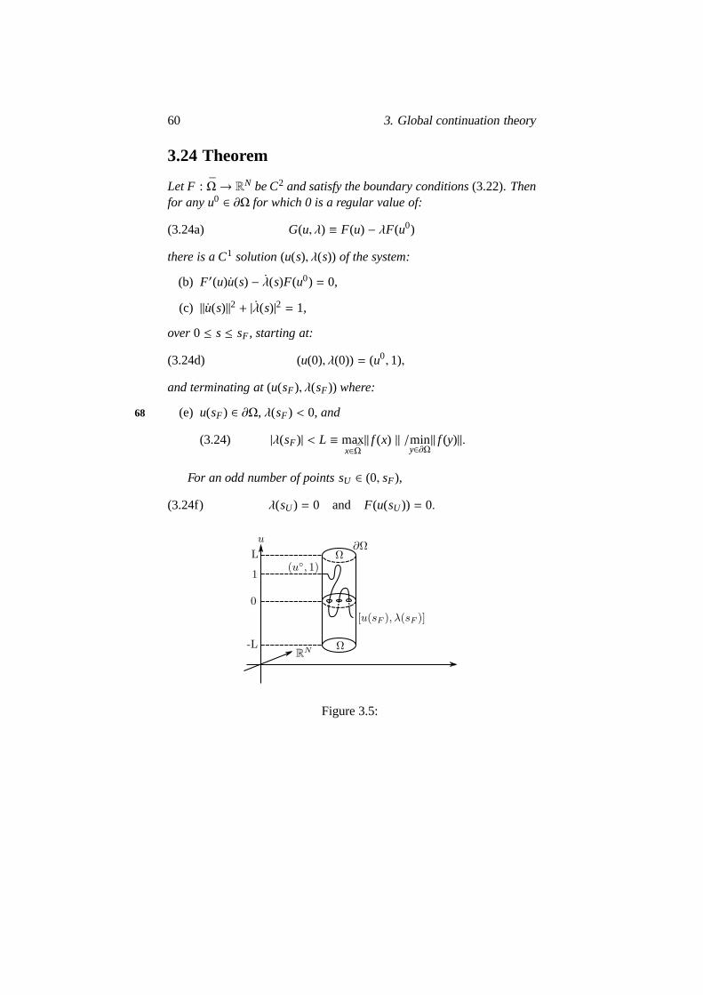
3.24 Theorem

Let F : Ω→ RN be C2 and satisfy the boundary conditions(3.22). Thenfor any u0 ∈ ∂Ω for which 0 is a regular value of:

(3.24a) G(u, λ) ≡ F(u) − λF(u0)

there is a C1 solution(u(s), λ(s)) of the system:

(b) F′(u)u(s) − λ(s)F(u0) = 0,

(c) ||u(s)||2 + |λ(s)|2 = 1,

over0 ≤ s≤ sF, starting at:

(3.24d) (u(0), λ(0)) = (u0, 1),

and terminating at(u(sF), λ(sF)) where:

(e) u(sF) ∈ ∂Ω, λ(sF) < 0, and68

(3.24) |λ(sF)| < L ≡ maxx∈Ω|| f (x) ‖ /min

y∈∂Ω|| f (y)||.

For an odd number of points sU ∈ (0, sF),

(3.24f) λ(sU) = 0 and F(u(sU )) = 0.

1

L

-L

0

Figure 3.5:

3.24. Theorem 61

Proof. In RN+1, we consider the cylinderK ≡ Ω × [−L, L], whereL isdefined as in (3.24d). See Fig. 3.5. Then for any fixedu0 ∈ ∂Ω, wehaveG(u, λ) , 0 on the bases ofK : λ = ±L andu ∈ Ω. But on thecylindrical surface ofK there is at least one solution of (3.24a), Viz. at(u, λ) = (u0, 1). Now 0 is a regular value and

∂G(u, λ)∂(u, λ)

|(u0,1) = [F′(u0),−F(u0)].

By assumption (3.22a),F′(u0) is nonsingular. Hence there is aC1

arc Γ(s) ≡ [u(s), λ(s)] which satisfies (3.24a,b,d). Takings as the ar-clength, we obtain (3.24c) also. Choose the sign of (˙u(0), λ(0)) so that 69

Γ(s) ∈ K for s> 0; that isu(0) atu0 points intoΩ. Continuity alongΓ(s)determines the orientation of the tangent (˙u(s), λ(s)) satisfying (3.24c)in the interior ofK. SinceL is so large thatG does not vanish for|λ| = L,the pathΓ(s) for s > 0 cannot meet the bases ofK. The pathΓ(s) can-not terminate in the interior since if it had an interior point must lie onΓ. Then the implicit function theorem gives a contradiction,since 0 isa regular value. ThusΓ(s) must meet the cylindrical surface ofK forsomes = sF > 0. Since the tangent (˙u(sF), λ(sF)) to Γ(s) at sF cannotpoint intoK, it follows thatu(sF) cannot point intoΩ at u(sF) ∈ ∂Ω.

Multiplying (3.24b) byλ(s) and using (3.24a):

λ(s).F′(u)u(s) − λ(s)F(u(s) = 0 onΓ.

F′(u) is nonsingular atu = u0 andu = u(sF). Therefore at points, wehave:

λ(s)u(s) = λ(s)(F′(u(s)))−1F(u(s))

Note thatλ(0) andλ(sF) are not zero, sinceF′(u(s)) is nonsingularfor s = 0 andsF. Now using the boundary condition (3.22b), We candeduce that

(3.25)λ(0)

λ(0)

λ(sF)

λ(sF)< 0.

Both λ(0)u(0)

λ(0)andλ(sF)

u(sF)

λ(sF)point out of (or into)Ω. But u(0)

points intoΩ andu(sF) does not, so (3.25) follows.


Now we will show thatλ(0)λ(sF) > 0 which impliesλ(0)λ(sF ) < 0. 70

Henceλ(sF) < 0 and so the theorem follows. We have:

Gu · u+Gλ · λ = 0

uT · u+ λλ = 1,

and from (3.12a,b):

λ(s) =detF′(u(s))

detA(s).

Now u0 andu(sF) are∂Ω. By assumption (3.22a),F′(u(s)) is non-singular for allu ∈ ∂Ω. Since∂Ω is connected, detF′(u(s)) has the samesign ats = 0 ands = SF . Also A(s) is nonsingular all alongΓ, as wehad seen in the proof of theorem 3.11. Henceλ(0) andλ(sF) have thesame sign and the proof is complete

Chapter 4

Practical procedures incomputing paths

4.1 Introduction71

We will consider the problem either in uniform formulation (4.1a) or informulation (4.1b):

G(x) = p whereG : RN+1→ RN;(4.1a)

G(u, λ) = P where,G : RN × R→ RN.(4.1b)

Definition. (a) A pathΓ = x(s) : x(s) ∈ Ω,G(x(s)) = p for all s∈ I issaid to be regular if RankGx(x(s)) = N for all sεI (Ω ⊂ RN+1).

(b) A pathΓ = (u(s), λ(s)) : u(s) ∈ Ω,G(u(s), λ(s)) = p for all s∈ I isregular if Rank [Gu(s),Gλ(s)] = N for all s∈ I (λ ⊂ RN).

Lemma 4.2. Rank[Gu,Gλ] = N if and only if either

(4.2) (i) Gu is nonsingular,

or

(4.2)(ii) (a) dim N(gu) = 1,

(b) Gλ < Range(Gu) ≡ R(Gu).

63

64 4. Practical procedures in computing paths

Proof. If (i) is true, then Rank [Gλ,Gλ] = N. In the other case,Gλ is nota linear combination of columns ofGu and sinceN(Gu) has dimension1, (N− 1) columns ofGu are linearly independent and henceN columns 72

of [Gu,Gλ] are linearly independent.Conversely, let Rank [Gu,Gλ] = N. Then either (i) holds or not. If

it does we are done. If not, then dimN(Gu) = 1 or else we cannot haveRank [Gu,Gλ] = N. But then we must also haveGλ 6 εR(Gu). Hence thelemma

Lemma 4.3. LetΓ be a regular path of(4.1a). Then there exists an opentube TΓ ⊂ Ω such that p is a regular value for G on TΓ andΓ ⊂ TΓ.

Proof. Take any pointx ∈ Γ, then there exists a minor matrix of rankN,sayM(x) of Gx(x(s)), such that detM(x) , 0. Recall that

detM(x) =N∏

j=1

k j(s)

wherek j(s) are all ten eigenvalues of the matrixM(x). Also k j(s)are smooth functions andk j(s) , 0 for j = 1, . . .N. Hence there willexists a neighbourhood ofx(s) in which the eigenvalues do not van-ish. Therefore in this neighbourhood, the minor is nonvanishing. Suchneighbourhoods exist at each point onΓ and so the tubeTΓ can be con-structed

Definition. A point (u(s), λ(s)) on Γ is said to be simple limit point (orsimple fold) if (ii a,b) of lemma 4.2 holds.

We have onΓ:

(4.4a) G(u(s), λ(s)) − p = 0,

so that:73

(4.4b) Gu(s)u(s) +Gλ(s)λ(s) = 0.

Note that at a fold points= s0, λ(s0) = 0 because

Gλ(s0) < R(Gu(s

0)).

4.1. Introduction 65

Henceu(s0) ∈ N(Gu(s0)) at a fold point. Since dimN(G0u) = 1 at

simple fold point (u0, λ0), we can take:

N(G0u) = spanφ,

andN(GoT

u ) = spanψ.

From (4.4b) we have:

G0uu+G0

λλ0+G0

uuu0u0+ 2G0

uλu0λ0+G0

λλλ0λ0= 0.

Multiplying throughout byψT and using the fact thatξ ∈ R(G0u) if

and only ifψTξ = 0, we get:

ψTG0λλ

0+ ψTG0

uuu0u0= 0,

asλ(s0) = 0 at a fold point. SinceG0λ< R(G0

u), we have:

ψTG0λ , 0,

and so

λ(s0) =−ψTG0

uuu0u0

ψTG0λ

.

But u(s0) = αφ for some scalarα. Hence: 74

λ(s0) = −α2−ψTG0uuφφ

ψTG0λ

.

If−ψTG0

uuφφ

ψTG0λ

, 0, then we say that (u0, λ0) is a simple quadratic

fold. We similarly define a ‘fold of orderm’ if λ(k)(s0) = 0 for allk = 1, . . .m− 1 andλm(s0) , 0.

Usual methods of computing paths fail at a fold point. So in thissection we present an algorithm for computing paths, that does not failat simple fold point.


4.5 Pseudoarclength Continuation

We already mentioned that at fold points on a regular path, Newton’smethod fails during natural parameter continuation. The main idea inpseudoarclength continuation is to drop the natural parametrization byλ and use some other parameterization. Consider the equation:

(4.6) G(u, λ) = 0,

whereG : RN × R → RN. If (u0, λ0) is any point on a regular path and(u, λ0) is the unit tangent to the path, then we adjoin to (4.6) the scalarnormalization:

(4.7) N(u, λ,∆s) ≡ u0T(u− u0) + λ0(λ − λ0) − ∆S = 0

This is the equation of a plane, which is perpendicular to thetangent(u0, λ0) at a distance∆s from (u0, λ0) (see Fig. 4.1). This plane willintersect the curveΓ if ∆sand the curvature ofΓ are not too large. That is75

we solve (4.6) and (4.7) simultaneously for (u(s), λ(s)). Using Newton’smethod this leads to the linear system:

(4.8)

[GU

u GUλ

uoTλ0

] [∆uU

∆λU

]= −

[GU

NU

]

Here GUu = Gu(uU , λU), GU

λ= Gλ(uU , λU), and the iterates are

uU+1= uU

+ ∆uU andλU+1= λU

+ ∆λU .

Figure 4.1:

4.5. Pseudoarclength Continuation 67

We will give practical procedures for solving the system (4.8) ona regular path. Recall that on such a pathG0

u may be nonsingular orsingular but the (N + 1) order coefficient matrix should be nonsingular.One proof of the nonsingular of the coefficient matrices in (4.8) can bebased on the following result (see: [7]).

Lemma 4.9. Let B be a Banach space and let the linear operatorA : 76

B× RU → B× RU have the form:

A ≡[

A BC∗ D

], where

A : B→ B, B : RU → B,

C∗ : B→ RU ,D : RU → RU .

(i) If A is nonsingular thenA is nonsingular if and only if:

(4.9a) D −C∗A−1B is nonsingular.

(ii) If A is singular with

(4.9b) dimN(A) = CodimR(A) = u,

thenA is nonsingular if and only if:

(c1) dimR(B) = u, (c2)R(B)⋂

R(A) = 0,

(c3) dimR(C∗) = u, (c4)N(A)⋂

N(C∗) = 0.(4.9c)

(iii) If A is singular withdim N(A) > u, thenA is singular

HereC∗ denotes the adjoin ofC. In our analysis we use only thecasesu = 1 andB ≡ RN. Then the conditions (4.9c) reduce to

(4.10) B < R(A) andCT< R(AT).

whereAT is the transpose ofA.

Note. Instead of using the earlier mentioned normalization (4.7), we canuse other relation. One obvious generalization of (4.7) is:

N ≡ θu0T(u− u0) + (1− θ)λ0(λ − λ0) − ∆s= 0, 0 < θ < 1;


77

Another type of normalization is:

N(u, λ, s) = θ||u(s) − u(s0)||2 + (1− θ)|λ(s) − λ(s0)|2 − (s− s0)2= 0.

Alternatively if we know nearby point onΓ say ats= s0 ands= s−1

then we can use:

N(u, λ, s) = θ

[u(s0) − u(s−1)

s0 − s−1

]T

(u(s) − u(s0))

+ (1− θ)[λ(s0) − λ(s−1)

s0 − s−1

](λ(s) − λ(s0)) − (s− s0) = 0.

This employs a scant rather a tangent. We call all of the abovepseudo arclength normalizations. For a references, see [18], [19].

4.11 Bordering Algorithm

We write the coefficient matrix of (4.8) in the form:

(4.12) A =

[A bcT d,

]

where,A is anN × N matrix, b, c ∈ RN andd ∈ R. Then we considerthe linear system:

(4.13) A(xξ

)=

(gγ

),

wherex, g ∈ Rn andξ, γ ∈ R.AssumeA andA are nonsingular. Then solve the linear systems:

(4.14a) Ay= b; Az= g.

Form the solution of (4.13) as:78

(4.14b) ξ =γ − cTz

d − cTy; x = z− ξy.

4.11. Bordering Algorithm 69

Note thatd − cTy = d − cTA−1b is the Schur complement ofA in A.Henced − cTy , 0 if A nonsingular. Thus ifA andA are nonsingular,then the bordering algorithm is valid.

Alternatively we may also write the system (4.13) as:

Ax+ bξ = g,

cT x+ dξ = γ.

To solve this, we can proceed by first eliminatingξ, if d , 0 to get:

ξ =1d

(γ − cT x).

Then forx we have:

(A−1d

bcT)x = g−γ

db.

Note that (A −1d

bcT ) is a rank 1 modification ofA. Hence from

the ‘Sherman-Morrison’ formula (see lemma 2.29 in Chapter 2), we can

easily determine the inverse of (A − 1d

bcT ), once we know the inverse

of A. In other words we can easily solve the linear system with the

coefficient matrix (A −1d

bcT). But this procedure requiredd , 0 while

the bordering algorithm does not. The nonsingularity ofA is requiredby both.

Now we will consider the case whenA is singular andA is nonsingu-lar. This occurs at simple points on solution paths (see equation (4.2,ii). 79

That is we assume:

(4.15a)(i) N(A) = spanΦ,(ii) b < R(A)

(iii) cT< R(AT).

These are precisely conditions (4.10) and are equivalent to:

(4.15b) ψTb , o andcTΦ , 0,


whereφ andψ are nontrivial solutions of :

(4.15c) Aφ = 0 and ATψ = 0.

We write the system (4.13) as :

A(Xoξo

) = (gγ),

wherex0, g ∈ RN andξ0, U ∈ R. That is:

Ax0 + bξ0 = g,

cT x0 + dξ0 = γ,(4.16)

Multiplying the first equation byψT , we get:

(4.17a) ξ0 =ψTg

ψTb.

Hence

(4.17b) Ax0 = g−ψTg

ψTbb ∈ R(A).

All solutions x0 of (4.17b) have the form:

x0 = xp + zφ,

wherexp is any particular solution of (4.17b) andz is obtained by sub-80

stituting the value ofx0 into the second equation of (4.16) to get:

z=γ − dξ0 − cT xp

cTφ.

Hence

(4.17c) x0 =

[xp −

cT xp

cTφφ

]+

(γ − dξ0

cTφ

)φ.

Hence the unique solution of (4.16) is given by (4.17a,c). Toeval-uate this solution we need the vectorsφ, ψ, xp and the inner productsψTg, ψTb, cTφ andcT xp.

The operational count to obtain these vectors is only one inner prod-uct more than the count required by the Bordering Algorithm.Thus thesolution (x0, ξ0) requires only two inner products more. We will showhowφ andψ can be obtained with half of a back solve each and hence atotal of one back solve.


Left and Right Null Vectors of A:

Assume thatA1 is anN×N matrix satisfying (4.15a) so that rank (A1) =N − 1. The with row and column interchanges determined by somepermutation matrices say,P andQ, the transformed matrix,

(4.18a) A ≡ PA1Q,

has anLU factorization:

(4.18b) A = LU ≡[

L 0ℓT 1

] [U u0T 0

]

HereL andU are lower and upper triangular matrices, respectively,81

of order (N − 1)× (N − 1) with:

L =

1· · · 1 0· · · · · · 1· · · · · · · · · 1· · · · · · · · · · · · 1

U =

u11 · · · · · · · · · · · ·u22 · · · · · · · · ·0 · · · · · · · · ·

· · · · · ·uN−1,N−1

Moreover:0, u, ℓ ∈ RN−1. Of course in actual calculations we do notget the exact zero element in the final diagonal position ofU. First wediscuss the null vectors and the we will discuss the inexact factorization.

SinceL is nonsingular,Aφ = 0 if and only if Uφ = 0. So withφ ∈ RN−1 andα ∈ R, we seekφ in the form

(4.19a) φ = α

(φ−1

), α , 0.

It follows because of the nonsingularity ofU that φ is uniquely de-termined by

Uφ = u.

In other words:φ = U−1u.

SinceU is in triangular form, we obtainφ and henceφ with only 82


one half of a back solve (for a system of orderN − 1). Similarly, the

nonsingularity ofU implies thatATψ = 0 if and only ifLTψ = β

(0−1

)for

β ∈ R. Thus we find that all nontrivial left null vectors are given by:

(4.19b) ψ =

(ψ−1

), β , 0,

andψ ∈ RN−1 is uniquely determined by:

LT ψ = ℓ,

ψ = (LT)−1ℓ.

Again ψ and henceψ are obtained with half of a back solve.

Almost Singular A

We already mentioned that in calculations we do not obtain the exactfactorization, but rather an approximation of the form:

(4.20) A = Aε = LεUε =

(L oℓT 1

) (U u0T ε

).

The quantityε will be an approximation to zero. If we use fullpivoting to determine the permutation matricesP andQ in (4.18a), thenunder appropriate conditions onA1 we can boundε by C10−t for t digitarithmetic whereC is a constant. The error analysis of Wilkinson [32]can also be used to estimate the magnitude ofε.

The basic assumptions that we make about the algorithm used to getthe form (4.20) and the error growth allowed, are summarizedby therequirement that in the singular case (4.15a):

maxj<N

∣∣∣∣∣∣ε

u j j

∣∣∣∣∣∣ ≪ 1.

In actual computations some precise relation must be used ifwe83


are to declare that we are in the singular case. With partial pivoting incolumns, one reasonable test is:

minj<N

∣∣∣∣∣∣u j j

u j−1, j−1

∣∣∣∣∣∣ > 102

∣∣∣∣∣∣ε

uN−1,N−1

∣∣∣∣∣∣ .

Of course the factor 102 may vary from case to case. A better theoryis needed here.

Now we use the factorization (4.20) and apply the Bordering Algo-rithm to solve (4.13). So consider

(4.21) a) Aεyε = b, (b) Aεzε = g,

with

b =

[b

bN

], g =

[g

gN

].

Now usingφ andψ obtained from (4.19a,b) withα = β = 1, we caneasily see that:

(a) yε =

[(L U)−1b

0

]+ψTbεφ

(b) zε =

[(L U)−1g

0

]+ψTgεφ

(4.22)

Now form (as in (4.14b))

(a) ξε =γ − cT(L U)−1g− 1

ε(ψTg)(cTφ)

d − cT(L U)−1b− 1ε(ψTb)(cTφ)

,

(b) xε =

[(L U)−1(g− ξεb)

0

]+

1ε

[(ψTg) − ξε(ψTb)]φ.

(4.23)

We must compare the solution (4.23) with the exact solution for the 84

singular case (4.17a,c). To do this, identify the particular solutionxp as:

xp ≡[(L U)−1(g− ξ0b)

0

].


Now we can expand (4.23) aboutε = 0 to obtain the results :

ξε = ξ0 + 0(ε),

xε = x0 + 0(ε).

In more detail we have :

ξε =ε(γ − cT(L U)−1g) − (ψTg)(cTφ)

ε(d − cT(L U)−1b) − (ψTb)(cTφ),

=ε(γ − cT (L U)−1g)

ε(d − cT(L U)−1b) − (ψTb)(cTφ)

−(ψTg)(cTφ)

ε(d − cT (L U)−1b) − (ψTb)(cTφ),

=ψTg

ψTb+ 0(ε) = ξ0 + 0(ξ).

Thus asε → 0, the first term of the right hand side of (4.23b) con-verges toxp. Also :

1ε

[ψTg− ξ(ψTb)]φ =1ε

[ψTg.ε(d− cT(LU)−1b) − ε(γ − cT(LU)−1g)ψTb

ε(d− cT(LU)−1b)(ψTb)(cTφ)

]φ

= (ψTb)

[d.ψ

TgψTb − γ + cT xp

]φ

ε[d− cT(LU)−1b

]− (ψTb)(cTφ)

=−dξ0 + γ − cT xp

cTφφ + 0(ε).

Hencexε = x0 + 0(ε).

Note that in the calculation the significant terms±(ψTg)(ψTb)(cTφ)85

cancelled each other. Hereξ0, x0 are the exact exact solutions whenε = 0.

Thus we find that the Bordering Algorithm can be used to solve(4.13) wheneverA is nonsingular. IfA happens to be singular, thenresults of some accuracy will be obtained only if a reasonable pivoting


strategy is used. Even in this case some accuracy loss must beexpecteddue to the cancellation of significant digits that occurs in forming x asin (4.14b). This cancellation is exactly analogous to the cancellation of

the1ε

terms inxε of (4.23b). If in the course of the calculations it is

recognized that we are at a limit point then the singularA algorithm canbe used and a more accurate numerical solution will result asno extrasignificant digits are lost (see [17] for more details). We will give somenumerical examples in the last chapter, in which we have usedthe abovealgorithm and they have performed well.

The Tangent Vectors

We will briefly describe how to compute the tangent vectors (˙u0, λ0).They must satisfy :

(a) Guu +Gλλ= 0,

(b) ||u||2 + |λ|2 = 1.(4.24)

First we consider regular points, whereGu is nonsingular. We findφ0. from:

(4.25) Guφ0 = −Gλ.

Then set: 86

(4.26) u = aφ0 and λ0 = a

wherea is determined from (4.24b) as :

(4.27) a =±1

√1+ ||φ0||2

.

The sign of a is chosen so that the orientation of the path is pre-served. More precisely, if (˙u−1, λ−1) is the preceding tangent vector thenwe require

uT−1u0

+ λ−1λ0 > 0.


Thus we choose the sign of ‘a’ so that

a[uT−1φ0 + λ−1] > 0.

Choosing the sign of a is very important in numerical calculations.If we do not choose the sign of a properly, either we will get trapped inthe iterations at some point or it will reverse the directionand hence itwill compute the same path already computed.

Another important point to recall in actual calculations isthat thequantity||u||2 is usually meant to approximate someL2 norm of the con-tinuous formulation of the problem. Thus the net spacing, say h, mustbe used to form for example :

||u||2 =J∑

j=1

hdu2j .

Here u j represent the components of ˙u and the underlying contin-uous problem is assumed formulated over a domain inRd. If this is87

not done the arclength definition||u||2 + λ2 is biased too much in theu-subspace andλ is not very significant.

We return to the case of a simple fold at whichGu is singular. Theanalysis of the case of almost singularA, (4.20)–(4.22), shows that weget in this case for the solution of (4.25), by setting

(4.28a) φ0 =

[φ0

ω0

], −Gλ =

[gγ

];

The result :

φ0 = −(L U)−1g+

(γ − ψT g

ε

)φ,

ω0 = −(γ − ψT g

ε

)≡β

ε(say).

(4.28b)

Using these results (4.28) in (4.26) and (4.27) we find that weindeedget the tangent to within 0(ε).

Chapter 5

Singular Points andBifurcation

5.1 Introduction88

First consider the problem in the uniform formulation, viz .

(5.2) G(X) = p.

In this formulation we will consider paths which contain singularpoints and give methods to jump over such points. This includes bifur-cation points in the general case.

5.3 Definition

A point X(s0) on a (smooth) solution path of (5.2) say,

Γab ≡X(s) : X(s) ∈ RN+1, G(X)(s)) = p, p ∈ RN, a < s< b

is a simple singular point ifs0 ∈ (a, b) and RankGx(X(s0)) = N − 1.Note that heres may be any parameter, it need not be arclength.

SinceGX is anN × (N + 1) matrix, at a simple singular pointX(s0), GX

has two independent null vectors, say,Φ1 andΦ2 in R(N+1). Withoutloss of generality we can require

ΦTi Φ j = δi j ; i, j = 1, 2,

77

78 5. Singular Points and Bifurcation

thus introducing an orthogonal system of co-ordinates forNGX(X(s0)).Now GT

X(X(s0)) is an (N + 1)× N matrix of rankN − 1, so that,

NGT

X(X(s0))= spanψ,

for some nontrivialψ ∈ RN.89

Tangents toΓab

From (5.2), it follows that:

GX(X(s))X(s) = 0.

Hence ats= s0, X(s0) has the form :

X(s0) = αφ1 + βφ2, α, β ∈ R.

Differentiating again we have :

GX(s)X(s) +GXX(s)X(s)X(s) = 0.

Now multiplying by ψT and evaluating ats = s0, the first termsvanishes and we have:

ψTGXX(s0)X(s0)X(s0) = 0.

Substituting forX(s0), we get :

(5.4a) a11α2+ 2a12αβ + a22β

2= 0.

Hereai j ’s are given by:

(5.4b) ai j = ψTGXX(s0)φiφ j .

Since (5.4a) is a quadratic equation, it follows that the roots are gov-erned by the discriminant:

(5.4c) ∆ = a212− a11a22

> 0, two real roots,

= 0, one real root,

< 0, no real root.

5.3. Definition 79

SinceΓab is a smooth solution path, it has at least one nontrivial90

tangent at each point onΓab. Hence the case∆ < 0 is not possible. Sothe following lemma holds.

Lemma 5.5. At a simple singular point X(s0) on a smooth solution pathΓab either∆ > 0 or ∆ = 0.

If ∆ > 0, then there exist two nontrivial tangents at a singular point.This suggests that bifurcation occurs at that point. Also itgives us anidea for constructing solution paths and switching over from one branchto another.

As in the earlier chapter, we adjoin some scalar normalization

N(X, s) = 0,

to the equation:G(X) = 0,

whereX ∈ RN+1, s ∈ R to obtain the augmented system fromRN+2 →R

N+1:

(5.6a) F(X, s) ≡[

G(X)N(X, s)

]= 0.

Using the normalization

(5.6b) N(X, s) = XT(s0)(X − X(s0)) − (s− s0),

we get:

(5.6c) FX(X(s)) =

[GX(X(s))XT(s0)

].

FX is an (N + 1) × (N + 1) matrix. In the previous chapter we proved91

that at a simple limit point, the augmented system is nonsingular (usingthe normalization in (5.6b)). AlthoughGX has a two dimensional nullspace, we will show thatFX has only one dimensional null space at asimple singular point.


Lemma 5.7. dim NFX(X(s0) = 1 at a simple singular point X(s0) ona solution pathΓab.

Proof. We use the notationFX(X(s0)) ≡ FX(s0) and suppose

FX(s0)φ = 0.

Then the firstN equations are:

GX(s0)φ = 0,

which implies that for someα0, α1ǫR:

φ = α0Φ1 + α1Φ2.

The last equation is :

XT(s0)φ = 0,

which implies by the orthogonality ofΦ1 andΦ2:

αα0 + ββ0 = 0.

That is:92

α0 : β0 = −β : α.

This shows that there is, upto a scalar factor, only one null vector ofFX(s0). This completes the proof of the lemma.

We recall that:

detFX(s0) =N+1∏

j=1

n j(s0),

wheren j(s0) are eigenvalues ofFX(s0). SinceFX(s0) has a one dimen-sional null space at least one of the eigenvalues is zero. We assume onlyone is zero. i.e. zero is an algebraically simple eigenvalues. Assume thatn1(s0) = 0 andn j(s0) , 0 for j = 2, . . .N + 1. Now consider detFX(X)for ‖ X − X(s0) ‖ small and let the corresponding eigenvalues ben j(X).Suppose

∇Xn1(X)|X=X(s0) , 0.

5.3. Definition 81

Then we can apply the implicit function theorem to show thatn1(X) =0 on a smooth manifoldM of dimensionN. Thus detFX = 0 on M. Ifthe solution path is transversal toM, i.e. the tangent at the point of in-tersection makes an acute angle with the normal to the manifold, thenthe path crossesM. So the sign of detFX(X(s)) changes along the path.Then theorem 3.17 allows us to conclude that the point of intersectionis a bifurcation point.

Now we compute the angle between the tangentX(s0) to Γab at s =s0 and the normal to the above manifoldM at s = s0, viz.∇Xn1(X(s0)).Let φ(X(s)) denote the eigenvector corresponding ton1(X(s)). Then 93

FX(s))Φ(X(s)) = n1(X(s))Φ(X(s))

Differentiating this expression and evaluating ats= s0, wheren1(X(s0)) =0, yields

FXXXΦ + FXΦXX =< ∇n1, X > Φ

LetNFT

X |s=s0 = spanΨ.

Then taking innerproduct withΨ,

< Ψ, FXXXΦ >=< ∇n1, X >< Ψ,Φ > .

To evaluate the required angle< ∇ni , X >, we need to findΦ andΨ.Lemma 5.7 shows

Φ = βΦ1 − αΦ2

Also we have

Ψ = (Ψ, 0), Ψ ∈ NGTX(X(s0))

and hence using the notations of (5.4a,b,c,),

< Ψ, FXXXΦ > =< Ψ,GXX(αΦ1 + βΦ2)(βΦ1 − αΦ2) >

= αβa11+ (β2 − α2)a12 − αβa22

= (β2 − α2)(a11α

β+ a12) = (β2 − α2)

√∆


Since ats= s0, zero is an algebraically simple eigenvalue ofFX(X(s0)),

< Ψ,Φ >, 0.

94

Thus we deduce that the required angle is not zero if∆ > 0 andhence the points= s0 on the solution path is a bifurcation point.

By choosing the basis vectors forNGX(X(s0)) suitably, the abovecomputation can be simplified considerably. For example, bytaking

NGX(X(s0)) = spanΦ1, X,

we get< Ψ, FXXXΦ >= a12

This is done in detail in the bifurcation theorem below.

5.8 Bifurcation Theorem

Let X0= X(s0) be a simple singular point on a smooth solution path

Γab = X = X(s) ∈ RN+1, G(X(s)) = p, p ∈ RN, sa < s< sb.

Let∆ > 0 and 0 be an algebraically simple eigenvalue of FX(X(s0))(defined as in(5.4c)and (5.6c) respectively). Then X0 is a bifurcationpoint onΓab

Proof. Consider the system:

F(X, s) ≡[

G(X)N(X, s)

]= 0

Heres is the parameter used to defineΓab. We will show thatF hasa bifurcation ats = s0 which in turn will prove thatG has a bifurcation95

at s= s0. Consider the normalization:

N(X, s) = X(s0)T [X − X(s0)] − t(s)

5.8. Bifurcation Theorem 83

wheret(s) is the distance betweenX(s0) and the projection ofX(s) ontothe tangent toΓab at X(s0). See Fig. 5.1.

Figure 5.1:

With the indicated normalization,X(s) is a solution ofF(x, s) = 0.We have :

FX(X(s)) =

[GX(s0)X(s0)T

]

At a singular pointGX has a two dimensional null space and thetangent vector,X(s0), is in NGX(s0). HenceX(s0) = αΦ1 + βΦ2, forsomeα, β ∈ R. We choose the basis vectorsΦ1 andΦ2 of NGX(s0)such thatα = 0, β = 1. We also proved thatNGX(s0) has dimension 96

one and hence by the choice ofX(s0) = Φ2 we must have:

FXX(s0)Φ1 = 0

Now consider the eigenvalue problem:

FX(X(s))Φ(s) = n(s)Φ(s).

At s = s0, one of the eigenvalues is zero, say,n(s0) = 0 and soΦ(s0) = Φ1. FX has a left null vectorΨT which is given byΨT

= (ΨT , 0)whereΨT is a left null vector ofG0

X. Now we can easily show that:

n(s0) =Ψ

TF0XXΦ1Φ2

ΨTΦ1=

a12

ΨTΦ1.


Sinceα = 0, β = 1 is a root of the equation:

a11α2+ 2a12αβ + a22β

2= 0

we must have:a22 = 0

Since∆ > 0, this implies thata12 , 0. Hence ˙n(s0) , 0. ThereforedetFX changes sign ats = s0. So by theorem 3.17,F and henceG hasa bifurcation atX(s0).

Note.This theorem gives conditions under which a point on the solutionpath is a bifurcation point. But we do not obtain two smooth branches ofsolution. This can be done using the Lyapunov-Schmidt method whichwe are not going to discuss here (Refer [4], [26]).

Now consider the parameter formulation of the problem:97

(5.9) G(u, λ) = 0

5.10 Definition

A point (u(s0), λ(s0)) on a solution pathΓab is a simple singular point ifand only if Rank[Gu(s0),Gλ(s0)] = N − 1.

At a simple singular point, since Rank [Gu(s0),Gλ(s0)] = N − 1,NGu(s0) has dimension either one or two. If it is one thenGλ(s0) ∈R(Gu) and if it is two, thenGλ(s0) < R(Gu). Conversely, if eitherNGu(s0) has dimension one andGλ(s0) ∈ R(Gu) or N(Gu(s0)) has di-mension two andGλ(s0) < R(Gu), then (u(s0), λ(s0)) is a simple singularpoint. So we have proven:

Lemma 5.11. The point(u(s0), λ(s0)) is a simple singular point if andonly if either:

(5.11a)(i) dim NGu(s0) = 1,

(ii) Gλ(s0) ∈ R(Gu).

or:

(5.11b)(i) dim NGu(s0) = 2,(ii) Gλ(s0) ∈ R(Gu).

5.10. Definition 85

This case (5.11b) is similar to the case we discussed in the uniformformulation, sinceN(Gu(s0)) has two independent null vectors and we98

can proceed as above. Now consider the case (5.11a) and let

NGu(s0) = spanΦ,

NGTu (s0) = spanΨ.

From (5.11a(ii)), the equation:

Gu(s0)φ0 = −Gλ(s0),

has a solution and it can be made unique by requiring thatφTφ0 = 0.Note that the tangent vector is

X(s0) =

[u(s0)λ(s0)

].

Then we have for someα, β ∈ R:

λ(s0) = β, u(s0) = αφ + βφ0.

where:

X(s0) = αΦ1 + βΦ2

Φ1 =(φ

0

), Φ2 =

(φ01

).

From (5.9) with (u, λ) = (u(s), λ(s)), we get on differentiating twiceand settings= s0:

G0uu0 +G0

λλ0 + (G0uuu0u0 + 2G0

uλu0λ0 +G0λλλ0λ0) = 0.

Multipling by ΨT , we get,

(5.12a) a11α2+ 2a12αβ + a22β

2= 0,

where now:

a11 = ΨTGuu(s0)φφ

a12 = ΨT [Guu(s0)φ0 +Guλ(s0)]φ

a22 = ΨT [Guu(s0)φ0φ0 + 2Guλ(s0)φ0 +Gλλ(s0)].

(5.12b)


99

Again if ∆ > 0, (5.12a) has two real roots and if∆ = 0, it has onereal root. It can be shown that∆ > 0, then each root (α∗, β∗) of (5.12a,b)generates a smooth solution are (u(s), λ(s)) for sands0 of the form:

u(s) = u0 + (s− s0)[α(s)φ0 + β(s)φ1] + (s− s0)2v(s),

λ(s) = λ0 + (s− s0)α(s),

where,

ΨTv(s) = 0,

α(s0) = α∗,

β(s0) = β∗.

For details see [7]. This result is well known in other forms.See[5], [26].

5.13 Continuation Past Simple Singular Points

Let Γab = X(s) : X(s) ∈ RN+1, G(X(s)) = 0, sa < s < sb be a smoothpath. Assume that ats = s0 ∈ (sa, sb), the pointX(s0) is an isolatedsimple singular point, that is rank ofGX(X(s)) = N in the intervals[sa, s0) and (s0, sb] and the rank isN − 1 ats= s0.

Let100

F(X, s) ≡[

G(X)N(X, s)

]= 0,

where,N(X, s) ≡ XT(sa)[X − X(sa)] − (s− sa).

We try to construct a solution using the Newton iteration method :

(5.14)(a) AU(s) ≡ FX(XU(s), s),(b) AU(s)[XU+1(s) − XU(s)] ≡ −F(XU(s), s),

U = 0, 1, 2, . . . ,

with the initial estimateX0(s) as:

X0(s) = X(sa) + (s− sa)X(sa).

5.13. Continuation Past Simple Singular Points 87

To assure convergence, we have to show thatX0(s) is in an appro-priate domain of convergence. Recall the Newton-Kantorovich theorem2.23: we get convergence under the assumptions that, for some s , s0

in (sa, sb):

(a) F(X(s), s) = 0,

(b) ||F−1X (X, (s), s)|| ≤ β(s),

(c) ||FX(X, s)−FX(Y, s)|| ≤ γ(s)||X−Y||, for all X,Y ∈ Bρ(s)(X(s)), ρ(s) >0,

(d) ρ(s) <2

3β(s)γ(s).

Of course ass→ s0, ||F−1X (X(s), s)|| → ∞. But in the case simple bi-

furcation point, it can be shown that||F−1X (X(s), s)|| ≤

M0

|s− s0|for some

M0 > 0, s , s0 (See [6]). This shows that there is a full conical neigh-bourhood, with positive semiangle about the solution are throughX(s0), 101

and vertex atX(s0), in which FX(Y, s) is nonsingular. See Figure 5.2.Note that the tangentX(sa) departs from one cone at the pointA andpenetrates atB the other cone. We have already seen that for all initialvalues within this conical neighbourhood, the iterates converge.Hencethis allows us to continue our procedure without any troubleat the sin-gular point. The pointX(s0) can be determined by a bisection procedurewith s1 = sa and sU < s0 < sU+1, for U = 1, 2, 3, . . . Each new tan-gent line through the new solutionX(sU) will have smaller chord lyingoutside the cone. In the limit the tangent throughX(s0) the bifurcationpoint, is entirely contained within the cone (locally). Thefinal configu-ration or a close approximation to it, gives one of the best techniques forcomputing the bifurcation branch by merely switching the tangent to beused in the normalization. See Figure 5.3. We will discuss later in thischapter how to find the new tangent


Figure 5.2:

Figure 5.3:

102

5.15 Properties at Folds and Bifurcation Points onPaths

For the parameter formulation

(5.16) G(u, λ) = p,

5.15. Properties at Folds and Bifurcation Points on Paths 89

we consider the eigenvalue problem:

(5.17)(a) Gu(s)φ(s) = n(s)φ(s),(b) ||φ(s)||2 = 1.

along a solution path of (5.16):

Γab ≡ (u(s), λ(s)) : G(u(s), λ(s)) = p, sa < s< sb

Note that at an algebraically simple eigenvalue,φ(s) andn(s) areC∞

functions ifG is C∞. Assume that the problem has a simple limit point103

or a simple singular point of type (5.11a) ats = s0 ∈ (sa, sb). Then wehave:

NGTu (s0) = spanψ,

NGu(s0) = spanφ,

for someψ, φ ∈ RN. SinceGu(s0) is singular and the null space isspanned byφ, we must have, for someφ(s), n(s):

n(s0) = o, φ(s0) = φ

Now differentiating (5.17a) twice and multiplying byψT and settings= s0, we get:

(5.18) ψT [Guu(s0)u(s0)φ +Guλ(s0)λ(s0)φ] = n(s0)ψTφ.

Observe that if the eigenvalue is algebraically simple thenψTφ , 0.So in this case we can solve for ˙n(s0). We use this in the proof of thefollowing lemma.

Lemma 5.19. Let (u(s0), λ(s0)) be a simple quadratic fold onΓab. As-sume that n(s0) = 0 is an algebraically simple eigenvalue of Gu(s0).Thenn(s0) , 0 anddetGu(s0) changes sign at s= s0.

Proof. At a fold point,

λ(s0) = 0, u(s0) = φ.


Hence we have: 104

n(s0) =ψTGuu(s0)φφ

ψTφ, 0,

becauseλ(s0) = ψTGuu(s0)φφψTGλ

, 0 and this implies thatψTGuu(s0)φφ , 0.Also if n j(s) are the eigenvalues ofGu(s), then,

detGu(s) =N∏

j=1

n j(s).

Without loss of generality, assume that :

n(s0) = n1(s0), n j(s0) , o∀ j = 2, . . .N.

Since then j(s) are continuous,n1(s) changes sing ats = s0 and allothern j(s), for j = 2, . . .N do not change sign in a neighbourhood ofs0. Hence the lemma follows

Lemma 5.20. Let (u(s0), λ(s0)) be a simple bifurcation points on asmooth pathΓab and n(s0) = 0 be an algebraically simple eigenvalueof Gu(s0). Let the discriminant∆ of equation (5.12a) be positive. Thenn(s0) , 0 and detGu(s) changes sign at s= s0 on one or both thebranches through the bifurcation point(u(s0), λ(s0)) for which λ(s0 ,

0).

See figures 5.4 a,b,c. The lemma states that the case shown in fig. 5.4cis not possible, sinceλ(s0) vanishes on both the branches. In fig. 5.4a,λ(s0) , 0 on both the branches, but in fig. 5.4b,λ(s0) , 0 onΓ+ andλ(s0) = 0 onΓ−

5.15. Properties at Folds and Bifurcation Points on Paths 91

(a) (b)

(c)

Figure 5.4:105

Proof. Let (α+, β+) and (α−, β−) be the roots of the quadratic equation(5.12a). At the bifurcation point,β+ andβ− gives λ(s0) correspondingto each one of the branches. Therefore ifλ(s0) = 0 along one of thebranches, then one ofβ+, β− say β+ = 0. Thenα+ cannot be zero.Hence from equation (5.12a), we have

a11 = 0

Since∆ > 0, a12 , 0. Also bothβ+ andβ− cannot vanish together.Thus at least for one branchλ(s0) , 0. Now for the nonvanishingβ,

αa11 + βa12 = β√∆ , 0.

From (5.18), we have 106


n(s0) =αa11+ βa12

ψTφ, 0.

Then detGu(s) changes sign as in the previous lemma.

Remark . In the case of simple limit points and simple singular pointsfor which (5.11a) holds,NGu(s0) has dimension one. The only dif-ference between these two types of points is that in the limitpoint caseGλ < R(Gu) and in the other caseGλ ∈ R(Gu). Hence ifψTGλ(s0) = 0,a bifurcation is effected and ifψTGλ(s0) , 0, afold is effected.

5.21 Exchange of Stability

The solutions of (5.16) are the steady states of the time dependant prob-lems of the form :

(5.22)∂U∂t= G(U, λ) − p.

Given an arc of solutionsu(s), λ(s) of (5.16), it is required to de-termine the stability of each point as a steady state of (5.22). To uselinearized stability theory we seek solutions of (5.22) in the form:

λ = λ(s)

U(t, s) = u(s) + ε exptx(s)φ(s)

‖φ(s)‖ = 1.

(5.23)

ExpandingG(U(t, s), λ(s)) aboutε = 0, we get:

(5.24a)∂U∂t= G(u(s), λ(s)) + εGu(u(s), λ(s)) exptx(s)φ(s) + 0(ε2).

But from (5.23), we have :107

(5.24b)∂U∂t= εn(s) exptx(s)φ(s).

Equating (5.24a) and (5.24b), sinceG(u(s), λ(s)) = 0, it follows that:

n(s)φ(s) = Gu(u(s), λ(s))φ(s) + 0(ε).

5.26. Switching Branches at Bifurcation Points 93

Hence we are led to the eigenvalue problem :

(5.25)(a) Gu(u(s), λ(s))φ(s) = n(s)φ(s),(b) ‖φ(s)‖ = 1.

If all eigenvaluesn = n(s) of (5.25) have Re(n(s)) < 0 for a givens, we say thatu(s) is linearly stable. If at least one eigenvalue hasRe(n(s)) > 0, thenu(s) is linearly unstable. If all the eigenvalue haveRe(n(s)) ≤ 0, with at least one equality holding, we say thatu(s) isneutrally stable.

Suppose (u(s0), λ(s0)) is a limit point as in lemma 5.19, thenn(s)changes sign as it crosses the points = s0. Hence if a smooth path ofsolutions has a simple quadratic fold ats = s0 as in lemma 5.19 andsolutions fors > s0 (or s < s0) are stable then they are unstable fors < s0 (or s > s0). Hence there is a change of stability ats = s0.Note that here we are not claiming that any branch of solutions is stableor not. We are only proving that if the solution branch is stable at oneside, then it is unstable on the other side. We cannot even conclude theconverse.

Similarly at a bifurcation point as in lemma 5.20, ˙n(s0) , 0 there 108

and detGu(s) changes sign ats= s0 on one or both the branches throughthe bifurcation point for whichλ(s0) , 0. Hence here also there maybe an exchange of stability on one or both the branches through thebifurcation point. Again here observe that we are not proving any branchof solutions is stable. But we do know that both arcs of one of thebranches cannot be stable.

5.26 Switching Branches at Bifurcation Points

Bifurcation points are solutions at which two or more branches of solu-tions of

(5.27) G(u, λ) − p = 0

intersect nontangentially. In this section we consider branch switchingonly at simple bifurcation points. For more details see [19].


Method I: An obvious way to determine branches bifurcating at (u0, λ0)is to determine the two distinct roots of (5.12a) and use themto deter-mine the distinct tangent vector in :

(5.28) u = αφ + βφ0, λ = β.

Then we can use our pseudoarclength continuation method to de-termine the different branches of solutions. If we know one branch ofsolutionsΓab, then we know the tangent, (˙u0, λ0), to the curveΓab at(u0, λ0) and this determines one root of (5.12a). Hence we can deter-mine the other tangent easily. Also note that in finding the values ofthe coefficientsai j of (5.12a) we need the derivativesG0

uu, G0uλ andG0

λλ.

But we can use the following approximation to these quantities which109

avoids the need for determining the second derivatives ofG.

aε11 =1εψT [Gu(u0

+ εφ, λ0) −Gu(u0, λ0)]φ,

= a11+ 0(ε),

aε12 =1εψT[Gu(u0

+ εφ0, λ0) −Gu(u0, λ0)]φ,

+ [Gλ(u0+ εφ, λ0) −Gλ (u0, λ0)],

= a12+ 0(ε)

aε22 =1εψTGu(u

0+ εφ0, λ

0) −Gu(u0, λ0)]φ0

+ 2[Gλ(u0+ εφ0, λ

0) −Gλ(u0, λ0)]

+ [Gλ(u0, λ0

+ ε) −Gλ(u0, λ0)],

= a22+ 0(ε).

Hereφ, ψ andφ0 are nontrivial solutions of

G0uφ = 0; GoT

u ψ = 0; G0uφ0 = −G0

λ, φTφ0 = 0.

Method II: In this method we assume that one branch through the bi-furcation point has been determined. Then the tangent (˙u(s0), λ(s0)) canalso be assumed to be known on this branch. The idea is to seek solu-tions on some subset parallel to the tangent but displaced from the bifur-cation point in a direction normal to the tangent but in a specific plane.


This method avoids the need to evaluate the coefficientsai j , i, j = 1, 2.Refore [19].

The solution branch (u1(s), λ1(s)) has a tangent in the direction given110

by (5.28). An orthogonal to this tangent in the plane spannedby (φ, 0)and (φ0, 1) is given by (5.28) but withα, β replaced by:

α = β(1+ ‖φ0‖2), β = −α‖φ‖2.

Then we seek solutions in the form :

u2 = u1(s0) + ε(βφ0 + αφ1) + v,

λ2 = λ1(s0) + εβ + η.(5.29a)

These are to satisfy:

G(u2, λ2) = p,

N(u2, λ2) ≡ (βφT0 + αφ

T)v + βη = 0.(5.29b)

We use Newton’s method to solve (5.29b) forv ∈ RN andη ∈ Rwith the initial estimate (v0, η0) = (0, 0). Hereε much be taken suffi-ciently large so that the scheme does not return to (u1(s0), λ1(s0)) as thesolution.

Method III (Lyapunov-Schmidt): Another way to determine a branchbifurcating from a known branch (u(s), λ(s)) at s = s0 is to apply aconstructive existence theory, as in [22]. We seek the bifurcated branchin the form :

u = u1(σ) + ε(φ + v), ψTv = 0

λ = λ1(σ).(5.30a)

Then we have:

(5.30b) G0uv− 1

εG(u1(σ) + ε(φ + v), λ1(σ)), ψTv = 0.

111

To ensure that the right hand side is inR(G0u), we try pickσ = s

such thath(s, ε, v) = 0, where,

(5.30c) h(s, ε, v) =

ψT [G0

uv− 1εG(u1(s) + ε(φ + v), λ1(s))], ε , 0,

ψT [G0uv−G(u1(s), λ1(s))(φ + v)]; ε = 0.


It follows thath(s0, 0, 0) = 0 and

h0s = hs(s0, 0, 0) = −ψT [G0

uuu1(s0) +G0uλλ1(s0)]φ

Then if h0s , 0 the implicit function theorem gives the function

s = σ(ε, v) and then it can be shown that (5.30b) has a unique solu-tion v = v(∈) for |ε| sufficiently small, using the contraction mappingtheorem.

The main difficulty in applying this method is in solvingh(s, ε, v) =0 for s at eachv = vU . If course if λ occurs linearly in the problemand it is used as the parameters, then this is easy. But in the case,modifications must be introduced. See [3], [8]. This method has alsobeen used for bifurcation from the trivial branch. See [31].

Method IV: Here we use a technique based on a modification of theCrandall and Rabinowitz [5] proof of bifurcation. Thus we seek solu-tions of the form (5.30a) and define

(a)g(v, s, ε) =

1εG(u1(s) + ε(φ + v), λ1(s)) if ε , 0

Gu(u1(s), λ1(s))(φ + v) if ε = 0

(b)N(v, s, ε) = ψTv.

(5.31)

112

Note thatg(0, s0, 0) = 0, N(0, s0, 0) = 0

and

A0=∂(g,N)∂(v, s)

∣∣∣∣∣0,s0,0)

=

[G0

u B0

ψT 0

],

where,B0 ≡

[G0

uuu1(s0) +G0uλλ1(s0)

]φ.

If ψT B0, 0, the by the lemma 4.9,A0 is nonsingular. Now the

implicit function theorem shows that :

g(v, s, ε) = 0,

N(v, s, ε) = 0.(5.32)


has a smooth solution (v(ε), ρ(ε)) for each|ε| ≤ ε0 and using this so-lution in (5.31a) yields the bifurcating branch of solutions. In solving(5.32) we never useε = 0 so that even when applying Newton’s method,second derivatives need not be computed.

Method V (Perturbed Bifurcation) : Observe that at a bifurcationpoint (u0, λ0), p is not a regular value forG. Since the set of all reg-ular values is dense, the idea of this method is to perturbp, sayp+ τq,q ∈ RN, ||q|| = 1, τ , 0, so thatp + τq is a regular value forG. Con-sider the two smooth branches of solutions through the bifurcation point 113

(u0, λ0). If we delete a small neighbourhood of (u0, λ0), we obtain 4different branches of solutions, sayΓ1, Γ2, Γ3, Γ4. Then consider theperturbed problem :

(5.33) G(u, λ) = p+ τq, q ∈ RN, ||q|| = 1, τ , 0.

Assumingp + τq is a regular value, this has no bifurcation andΓi,i = 1, 2, 3, 4 will simply be perturbed and will yield smooth nearbybranches of solutions of (5.33). These branches can be connected in 3ways. See Figs. 5.5 a,b,c.

Case (i) : Here if we are starting from a solution onΓ1, we will get aperturbed solution onΓ′1 and then we can continue alongΓ′1 to Γ′4 whichis the perturbed branch ofΓ4. Similarly fromΓ2, we will obtainΓ′2 andΓ′3 [Fig. 5.5a].

Case (ii) : In a similar manner we can handle this case also (see Fig. 5.5b).

Case (iii) : In the cases (i) and (ii) we can determine the other brancheswithout any difficulty. Our claim is that the case (iii) doesn’t happen.To see this we have to study further about fold following which we aregoing to describe in the next section. There we will considerthe problem(5.33) as a two parameter, (λ, τ) problem and will give an algorithm toobtain a fold .


(a) (b)

(c)

Figure 5.5:114

5.27 Multi Parameter Problems (Fold Following)115

We recall the two examples described in the introductory chapter onpopulation dynamics. We examined the steady state solutions of:

dξdt= −ξ2

+ λξ + τ,

dξdt= −ξ3

+ λξ + τ,

that is the solution of:

(1) − ξ2+ λξ + τ = 0,

(2) − ξ3+ λξ + τ = 0,

5.27. Multi Parameter Problems (Fold Following) 99

Example 1.−ξ2+ λξ + τ = 0.

We note that in the (λ, τ) plane there is a curve across which thenumber of solutions change. This curve is a fold. See the solution sur-face sketched in fig. 1.4.

Example 2.−ξ3+ λξ + τ = 0,

In Fig. 1.8 we show a curve in the (λ, τ) plane which has a cusp atthe origin; as (λ, τ) crosses this curve the number of solutions changes.Look at the solution surface in Fig. 1.12. This curve is a foldon thesolution surface.

Hence determining a fold is very important. Other interesting phe-nomena may occur along the folds. The solutions lie either tothe leftof the fold curve or to the right of the fold curve. In the latter case,(Fig. 5.6a) the fold point is known as a hyperbolic point and in the for-mer case (Fig. 5.6b) it is called an elliptic point. Suppose the fold point 116

is at (u0, λ0, τ0). In the elliptic case ifτ > τ0 we have no solution and onthe other hand ifτ < τ0, we obtain a closed loop of solutions. A closedloop of solutions is known as an ‘isola’. In the second case asτ changesfrom τ0 we get different branches of solutions. For a unified theory ofperturbed bifurcation and isola formation see [21].

FOLD

ISOLA

FOLD

(a) hyperbolic pt (b) elliptic pt

Figure 5.6:

Now letτ = τ0 and assume that there is a simple quadratic fold with


respect toλ at (u0, λ0). We haveG(u0, λ0, τ0) = p and

(5.35)(a) N(G0

u) = spanφ0, for someφ0 , 0,(b) G0

λ< R(G0

u) = v ∈ RN : ψT0 v = 0.

Hereψ0 is a nontrivial solution of:

(5.35) (c)G0Tu ψ0 = 0,

and at a simple quadratic fold:117

(5.35) (d)a = ψT0G0

uuφ0φ0 , 0.

Now consider the extended system:

F1(u, ψ.λ, τ) ≡

G(u, λ, τ) − pψTGu(u, λ, τ)ψTG0

λ− 1

= 0.

HereF1 : R2N+2→ R2N+1. This system can be written as:

(5.36) (a)F(U, τ) = 0,

where

(5.36) (b)U =

uψ

λ

andF ≡ F1. Note that (u0, ψ0, λ0, τ0) is a solution of this system. Weuse another formulation:

(5.37a) F2(u, ψ, λ, τ) ≡

F(u, λ, τ) − pGu(u, λ.τ)φℓTφ − 1

= 0,

whereℓ is such that

(5.37b) ℓTφ0 = 1.

This can also be written in the form (5.36) withF ≡ F2. In this118

letter case, we have the following theorem

5.27. Multi Parameter Problems (Fold Following) 101

Theorem 5.38.At a simple quadratic fold(u0.λ0, τ0):

F0U=

∂F∂(u,Φ, λ)

∣∣∣∣∣(u0,Φ0,λ0)

=

G0u 0 G0

λ

G0uuΦ0 G0

u G0uλΦ0

0 ℓT 0

is nonsingular.

Proof. AssumeF0UΦ = 0, for someΦ =

pqr

∈ R2N+1

That is

(5.39)(a) G0

U p+ rG0λ= 0,

(b) G0uuΦ0p+G0

uq+G0uλΦ0r = 0,

(c) ℓTq = 0.

Multiplying (5.39a) byψT0 and using (5.35 b,c), we getr = 0. Hence

G0up = 0. This shows thatp = αΦ0, for someα ∈ R. So (5.39b) implies

thatαψT

0G0uuΦ0Φ0 = αa = 0.

So that by (5.35d),α and hencep = 0. This impliesG0uq = 0. Hence

q = βΦ0 for someβ ∈ R. But by (5.39c) we getβℓTΦ0 = 0. Hence by

(5.37b),β andq = 0

Now we can apply the implicit function theorem to obtain

u = u(τ)

Φ = Φ(τ)

λ = λ(τ)

for |τ − δ| < δ, for someδ > 0. The arc (u(τ), λ(τ), τ) ∈ RN+2,, τ ∈ 119

(τ0 − δ, τ0 + δ) is part of the fold curve. We can also use some otherparametrization,s, to to obtain the solution in the form:

u = u(s)

Φ = Φ(s)


λ = λ(s)

τ = τ(s).

Now we will show how to use the Bordering Algorithm to find theNewton iterates applied to solve (5.37a). The linear systemhas the form:

(5.40) LX =

g∼γ

Here

L ≡ FU ≡

A b∼

c∼

T 0

, X ∈ R2N+2, g∼∈ R2N, γ ∈ R,

where

A ≡[A 0B A

]with A = G0

u, B = G0uuΦ0.

First solve:

Av∼= b∼, b∼, v∼∈ R2N,

Aω∼= g∼, g∼, ω∼∈ R2N.

120

Then form:

ξ =

γ − c∼

Tω∼

c∼

Tv∼

,

andx∼= ω∼− ξv∼.

Note that the system:

A

[y1

y2

]≡

[A 0B A

] [y1

y2

]=

[γ1

γ2

],

can easily be solved as follows:

5.41. Paths of Periodic Solutions and Hopf Bifurcation 103

First solveAy1 = γ1,

and thenAy2 = γ2 − By1.

Hence it follows that the system (5.40) can be solved by solvingfour systems the same coefficient matrixA. So we need do only oneLUdecomposition ofA and then four backsolves. See the Ref. [33] andalso [15].

5.41 Paths of Periodic Solutions and Hopf Bifurca-tion

121

In this section we will discuss the periodic solutions of thesystem ofODE depending on a parameter:

(5.42)dydt= f (y, λ).

First we will briefly describe Poincare’s method for containing peri-odic solution branches and then we discuss Hopf bifurcation. We do notgive a detailed description of these things. A good reference for Hopfbifurcation is [25].

We seek periodic solutions of (5.42). Suppose forλ = λ0 that y∼o

(t)

satisfies (5.42) andy∼o

(t+T0) = y∼o

(t), for someT0 > 0 and for allt. Then

y∼o

(t) is a periodic solution (5.42). Since this system is autonomous, for

anyσ, the translation ofy∼o

(t). viz.

y∼(t) = y

∼o(t + σ),

is also a periodic solution. We seek periodic solution whenλ is pertubedfrom λ0

Substitutingy∼o

(t) in (5.42) and differentiating we get:

ddt

y∼o

(t) = [ fy( y∼o

(t), λ0)] y∼o

(t).


LetA0(t) = [ fy( y

∼o(t), λ0)].

Then we can write

[ddt− A0(t)] y

∼0(t) = 0.

122

Hence the linearised operatorddt− A0(t) has a nontrivial periodic

solutions y∼0

(t). In the case of nonautonomous system this is not in gen-

eral true. Then we have to assume thatf (t, y, λ) is periodic, with periodT(λ). Then in general the linearized problem does not have nontrivialperiodic solution and the continuation inλ can be done yielding solu-tions with periodT(λ). In our case (5.42),f has all possible periods int.

Consider the periodic solutiony∼0

(t) of (5.42). At t = t0 = 0, y∼0

(0)

is some arbitrary point inRN and letπ ⊂ RN be the plane which isperpendicular to the tangent, ˙y

∼0(0) aty0(0). That is:

π = ξ∼∈ RN : y

∼o(0)T (ξ

∼− y∼o

(0)) = 0

Consider any pointξ∼επ in some small neighbourhood ofy

∼o(0) and

look at the solution curve of (5.42) passing through this point ξ∼. Sup-

pose the curve intersects this planeπ after sometime, then this point ofintersection is the image ofξ

∼under the poincare map. For the existence

of Poincare map see [25]. From the definition it is clear that the periodicsolution of (5.42) corresponds to the fixed points of the Poincare map.

Consider the initial value problem:

(5.43)(a) dy

dt =f (y,λ),

(b) y∼(0) = ξ

∼∈ RN.

Let y∼= y∼(t, ξ∼, λ) be the solution of (5.43), for (ξ

∼, λ) ∈ Bρ( y

∼o(0), λ0)123


for someρ > 0. The problem thus reduced to: findξ∼

andT such that :

(5.44)(a) y

∼(T, ξ∼, λ) − ξ

∼= 0,

(b) y∼o

(0)T [ξ∼− y∼o

(0)] = 0.

These are (N+ 1) equations inN+ 1 unknowns. Observe that atλ =λ0, we have the solutionξ

∼0= y∼o

(0), T = T0. We expect solutions forT

nearT0. We can apply the implicit function theorem if the Jacobian of(5.44) with respect to (ξ

∼,T) is nonsingular. The Jacobian at (ξ

∼0,T0, λ0)

is given by:

∂

∂(ξ∼,T)

y∼(T, ξ∼, λ) − ξ

∼y∼o

(0)T [ξ∼− y∼o

(0)]

≡(Y0 − I ) y

∼o(0)

y∼o

(0)T 0

≡ A.

HereY0= Y(T0, ξ

∼0, λ0), whereY satisfies :

(5.45)(a) dY

dt − A0(t)Y = 0,(b) Y(0) = I .

All solutions ofdvdt− A0(t)v = 0 are the form:

v∼(t) = Y(t)ζ

∼, ζ∼∈ RN,

and the solution is periodic if and only if:

[Y(T0) − I ]ζ∼= 0.

Already we know that ˙y∼o

(t) is a nontrivial periodic solution. Hence

Y(T0) has an eigenvalue unity. Now we will assume that 1 is a simpleeigenvalue ofY(T0). Under this hypothesis, we will prove that: 124

Lemma 5.21. A is nonsingular.


Proof. SupposeA

ζ∼z

= 0. Then

(5.47a) [Y(T0) − I ]ζ∼= −zy

∼o(0).

Multiplying throughout byY(T0)− I , since (Y(T0)− I ) y∼o

(0) = 0, we

get:

(5.47b) [Y(T0) − I ]2ζ∼= 0.

This shows that ifz, 0, then 1 is not a simple eigenvalue. Thus wemust havez= 0. Now the second equation gives:

y∼o

(0)Tζ∼= 0.

But [Y(T0) − I ]ζ∼= 0 implies thatζ

∼is a multiple of y

∼o(0). i.e.

y∼o

(0)T y∼o

(0) = 0. Hence we must haveζ∼= 0. Thus the proof is complete

We can solve the initial value problem (5.43) numerically The maindifficulty in applying such numerical method is that the numerical tra-jectory will blown up if the continuous orbit is not stable. Even in thestable case there may exist unstable orbits arbitrarily near to stable or-bits and these cause trouble. In many cases of course this “shooting”method works fine.

We can write the equation (5.44) in the form:

(5.48) G(u, λ) = 0,

whereu = (ξ∼,T). Here also we can do all the analysis of folds, bifurca-125

tions, stability etc. as before. We can also compute paths ofsolutions of(5.48) and hence paths of periodic solutions of (5.42).

We can formulate the continuous problems as follows, after scalingtime by the period,T:

(5.49) G(y∼(t), ξ∼,T, λ)

dydt − T f(y

∼, λ)

y∼(1)− ξ

∼y∼o

(0)T (ξ∼− y∼o

(0))

= 0.


HereG : B× RN × R2→ R × RN × RN × R. Now

∂G∂(y∼, ξ∼,T)≡

[ddt − TA(t, λ)

]0 f (y

∼, λ)

0 Y0 − I y∼T

(1)

0 y∼o

(0)T 0

HereA(t, λ) = fy(y∼(t), λ). As is lemma it can be shown that

∂G∂(y∼, ξ∼,T)|

y∼= y∼o

(t)

ξ∼= y∼o

(0)

T = T0

is nonsingular if 1 is a simple eigenvalue of Y0.We consider finite difference approximations to (5.49). We use a

uniform net (but this can easily be changed):

t j = jh, h =1M,

whereM is the number of partitions of the unit time interval. 126

t0 t1 t j−1 t j tM

Let u j be an approximation tou(t j ). We can approximate (5.49) as:

Gh(uh,T, λ) ≡

...

u j − u j−1 − Th f(

12(u j + u j−1), λ

)

...

u0 − uN

ξoT(uN − ξ0)

= 0.

This is a system ofMN + N + 1 equations inMN + N + 1 un-knowns. Here again we can apply the implicit function theorem to ob-tain (uh(λ),T(λ)) if h is sufficiently small. Here again there may exists


folds, bifurcations (Hopf bifurcation) etc. Hopf bifurcation is the bifur-cation of periodic solution orbit steady state solutions. Refer [14] and[10] for details.

Look at the steady states of (5.42). i.e. solutions off (y, λ) = 0. LetΓ0 = y(λ) be a solution branch. Eigenvalues of the linearized problemabout states determine the stability of these orbits as solutions of (5.42).127

So consider the eigenvalue problem:

A(λ)φ(λ) = η(λ)φ(λ)

Here A(λ) = fy(y(λ), λ). SinceA(λ) is real, the eigenvalues willoccur as complex conjugate pairs. Assumeη1(λ) = α(λ) + iβ(λ) andη2(λ) = α(λ)− iβ(λ). We know that at fold points, some real eigenvalueschange sign. Also if the real part of any eigenvalue changes sign, theremay be a change of stability. We examine the case of the even number,infact two complex eigenvalues changing sign of the real part.So assumeα(λ0) = 0, α(λ0) , 0 andβ(λ0) , 0. Then theHopf bifurcation theorem[see [25]] states that a periodic solution branch bifurcates from Γ0 atλ = λ0. Let

φ(λ) = a(λ) + ib(λ).

Substituting this in (??), we get:

Aa= αa− βb,

Ab= αb+ βa.(5.51)

At Hopf bifurcation, we haveα(λ0) = 0. Then look at the system(5.52a) for the unknowns (y, a, b, β, λ).

(5.52a)

f (y, λ)

fy(y, λ)a+ βb

fy(y, λ)b− βa

= 0.

This is a system of 3N equations in 3N + 2 unknowns. So we add


two normalizations to obtain a system of (3N + 2) equations, viz:

(5.52b)

f (y, λ)

fy(y, λ)a+ βb

fy(y, λ)b− βa

aTa+ bTb− 1

ℓTa− 1

= 0.

128

The choice of the unit vectorℓ need only satisfyℓTa(λ0) = 1.Here also we can apply numerical schemes to directly computepoints

of Hopf bifurcation. In the next chapter we will give some examples inwhich we employed various schemes that are discussed in the previouschapter.

Chapter 6

Numerical Examples

6.1 Introduction129

We present here in some detail, a few worked-out examples showinghow the techniques discussed in the lectures are actually employed. Un-fortunately we do not show all the procedures, but it should not be dif-ficult for the interested reader to try out the missing ones. We use pathfollowing via Euler-Newton continuation in both the natural parameterformulation and in the Pseudoarclength variant. Folds are circumventedby switching from the natural parameter to Pseudoarclengthwhen spe-cific tests tell us to do so. Then we switch back after the fold has beentraversed. We jump over bifurcation points easily and indeed must con-tinuously test to see if we must return to locate the folds or bifurca-tion points. We also locate the singular points accurately and switchbranches at the bifurcation points. Multiparameter problems are alsotreated.

The basic logic of our code is illustrated by a simple flow diagram.The numerical schemes employed are given. Details of the tests usedand some indication of how they performed are given below. Sev-eral problems have been solved and we show graphs of solutionpathsfor some of these problems. Some actual computer listings ofconver-gence data, steplength changes, accurate location of foldsand bifurca-tion points are included with explanation.

111

112 6. Numerical Examples

6.2 Problems and Difference Schemes130

Due to limitations of computing power available for these tests, we con-sider only O.D.E. problems. They are of the form:

(6.3) Lu ≡d2u

dx2+ p(x)

dudx= f (u, x, λ, τ, in (0, L)

subject to two point boundary conditions of the form:

(6.4)(a) B0u ≡ q0 u(0)+ r0

dudx

(0) = s0,

(b) BLu ≡ qL u(L) + rLdudx

(L) = sL.

The nonlinearities were of the semilinear form. No conceptual dif-ficulties occur if they are allowed to be quasilinear, i.e.f is in the form

f

(u,

dudx, x, λ, τ

). We use uniform grids of spacing

(6.5a) h =LN,

to define the netpointsx jN0 as :

(6.5b) x0 = 0, x j+1 = x j + h, j = 0, 1, . . .N − 1.

The usual centred difference scheme is employed, sometimes mod-

ified if singular coefficients occur(i.e. : p(x) =

mα

)or improved to get

fourth order accuracy ifp(x) = 0. If either r0 , 0 or rL , 0, we intro-duce exterior points atx−1=−h andxN+1 = L + h respectively. Denotingthe discrete approximation tou(x j ) by u j and using the finite differenceoperators:

D+u j ≡u j+1 − u j

h; D−uj ≡

u j − u j−1

h; D0u j ≡

u j+1 − u j−1

h.

Our basic difference approximation to (6.3) atx j is given by:131

(6.6) Lhu j ≡ D+D−u j + p(x)D0u j = f (u j , x j , λ, τ); j = 0, 1, . . .N.

6.2. Problems and Difference Schemes 113

The boundary conditions (6.4) are approximated as:

(a) Bh0uL ≡ q0u0 + r0D0u0 = s0,

(b) BhLuL ≡ qLuN + rLD0uN = sL,

(6.7)

The scheme in (6.6) forj = 0 and (6.7a) both involveu−1. Thisquantity is then eliminated using the two equations to get one relationbetweenu0 andu1. A similar treatment using (6.6) atj = N and (6.7b)eliminatesuN+1 and retains one equation inuN anduN−1. The systemthus reduced consists ofN + 1 equations in as many unknownsu j , j =0, . . .N. If r0 = 0 and (or)rL = 0, we do not impose (6.6) forj = 0and (or) j = N. The corresponding elimination need not be done and weagain getN + 1 equations in the same number of unknowns. We couldalso eliminateu0 and (or)uN. In this case we not bother to do that in ourdescription here.

The difference scheme in (6.6), (6.7) has second order accuracy. Ifthe continuous problem (6.3), (6.4) has an isolated solution U0 (say, forfixed λ, τ) and if p(x) and f are smooth, then it is known that, for suf-ficiently smallh, the discrete problem (6.6), (6.7) has a unique solutionu j in some sphere inRN+1 aboutu0(x j) and further it satisfies:

||u0(x j) − u j || = 0(h2).

Similar results also apply to the entire solution branches of (6.3), 132

(6.4) containing simple fold and bifurcation points. However there maybe some degradation of accuracy at these special points; this is discussedmore thoroughly in the expanded version of these notes.

If p(x) ≡ 0, we can easily get fourth order accurate, three pointschemes, using Collatz’s device as follows. Taylor expansions give:

D+D−u(x j) =d2u

dx2(x j) +

h2

12d4u

dx4(x j) + 0(h4).

Sinceu(x) satisfies:

d2u

dx2= f (u(x), x, λ, τ),


we have:

D+D− f (u(x j ), x jλ, τ) =d4u

dx4(x j) + 0(h2),

and thus we get:

D+D−u(x j ) −h2

12D+D− f (u(x j), x j , λ, τ) =

d2u

dx2(x j) + 0(h4).

Thus in place of (6.6) we use, whenp(x) ≡ 0 :

(6.8) Lhu j ≡ D+D−u j −112

( f j+1 + 10f j + f j−1), j = 0, 1, . . .N.

Here we have used the abbreviations:

f j ≡ f (u j , x j , λ, τ).

We can employ this device even when we have the mixed boundaryconditions (6.4). That is even whenr0 , 0 and (or)rL , 0. This doesnot seem to have been stressed before, so we indicate the details. Again133

Taylor expansions give:

D0u(x j) =dudx

(x j) +h2

12d3u

dx3(x j) + 0(h4).

Here the factorh2/12 occurs because we useD0 to approximated/dx and 2.3! = 12. Previously this factor came 4!/2. In any event now

D0d2u

dx2(x j) =

d3u(x j)

dx3+ 0(h3).

Using (6.3) withp(x) ≡ 0 atx = x j, in the above, we get

D0u(x j) −h2

12D0 f (u(x j ), x j , λ, τ) =

dudx

(x j) + 0(h2).

With x j = x0, andx j = xN, we replace (6.7) by :

(a) Bh0u0 ≡ q0u0 + r0D0(u0 −

h2

12f0) = s0,

(b) BhLuN ≡ qLuN + qLuN + rLD0(uN −

h2

12fN) = sL,

(6.9)

6.2. Problems and Difference Schemes 115

Now (6.9a) and (6.8), forj = 0, both contain non-zero multiples

of (u−1 −h2

12f−1) which can be eliminated between these two equations.

A similar treatment with (6.9b) and (6.8) forj = N eliminates (uN+1 −h2

12fN+1). The result is againN + 1 equations in the basic unknownsu j ,

j = 0, 1, . . .N and the tridiagonal structure of the system is retained [seethe equation (6.10) below]. Of course ifr0 = 0 and (or)rL = 0, weneed not bother with the above procedure atj = 0 and (or) j = n. Soin either of those cases, we need not impose (6.8) forj = 0 and (or)

j = N respectively. Even if the elimination of (u−1−h2

12f−1) etc. are not

performed we get enhanced accuracy, but the system structure is not as 134

elegant.

In the case of singular coefficients, (i.e:p(x) =mxα, 0 < α ≤ 1) we

modify the scheme as follows. Forj = 0 we replace (6.6) by:

(m+ 1)D+D−u0 = f0, if α = 1,

andD+D−u0 = f0 if 0 < α < 1.

These follow fromux(0) = 0 and hence :

limx→0

(uxx +mxα

ux) =

(m+ 1)uxx(0), if α = 1,

uxx(0), if 0 < α < 1.

We get only second order accuracy but the error expansion atx = 0proceeds in power ofh2.

All the difference schemes we have described can now be incorpo-rated into the general form:

g j(u j−1, u j , u j+1, λ, τ) ≡ α ju j−1 + β ju j + γ ju j+1 − α j f j−1

− β j f j − γ j f j+1 − δ j = 0, 0 ≤ j ≤ N.(6.10a)

Of course we always have :

(6.10b) α0 = α0 = γN = γN = 0,


and hence :

(6.10c) g0 ≡ g0(u0, u1, λ, τ); gN ≡ gN(uN−1, uN, λ, τ).

The system (6.10) is our finite dimensional problem which we canwrite in the vector form:135

G(u, λ, τ) =

g0

g1...

gN

= 0.

Thus our general finite dimensional problem is fromRN+3 to RN+1.Note that it is a nonlinear three term recursion, terminatedat j = 0 andj = N with two term relations.

Of paramount importance are the derivatives ofG with respect tou,λ andτ. The jth row of the Jacobian matrixGu is given by theN + 1vector:

∂gi

∂u∼

= (0, . . . 0, a j , b j , c j , 0, . . . 0), j = 0, . . .N.

ThusGu is a tridiagonal matrix withb j on the diagonal,a j andc j

are below and above the diagonal respectively. In standard notations forsuch matrices we have:

(6.11) Gu(u, λ, τ) ≡ [a j , b j , c j ]N0 .

Differentiating (6.10a) we get that :

a j ≡∂g j

∂u j−1= α j − α j( fu) j−1,

b j ≡∂g j

∂u j= β j − β j( fu) j ,

c j ≡∂g j

∂u j+1= γ j − γ j( fu) j+1, 0 ≤ j ≤ N.

(6.12)

The tridiagonal form of (6.11) becomes clear from (6.10b)136

6.16. Algorithm and Tests 117

and (6.12). Here we use the obvious notation :

( fu) j =∂ f∂u

(u j , x j , λ, τ).

Theλ andτ derivatives are not sparse; we have :

(6.13) Gλ =

...

gλ, j...

,

where,

gλ, j = −α j( fλ) j−1 − β j( fλ) j − γ j( fλ) j+1, 0 ≤ j ≤ N.

A similar set of relations defineGτ.To complete the detailed specification of any of our problems, we

need only to give:

(6.14) L, p(x), f (u, x, λ, τ), (q0, r0, s0), (qL, rL, sL).

When these are given, we examinep(x), r0 andrL to find out whichof the schemes we have described is to be employed. Then the constants

(6.15) (α j , β j , γ j , α j , β j , γ j , δ j), 0 ≤ j ≤ N

are determined. Now only the net spacing or integerN of (6.5a) need begiven. We give the coefficients of (6.15) in table I for some of the most137

basic cases to be tested.

6.16 Algorithm and Tests

The following are the main steps for computing the solution branchstarting from a known initial solution (uo, λo).

Step I. Determination of the unit tangent to the path, viz±(u, λ)

Step II. Choice of :


(i) the tangent direction;

(ii) steplength, along the path;

(iii) continuation method; natural parameter (n · p) or pseudoarclength(p · a).

Step III. Construction of the initial iterate : either for (n · p) :

u(1)= uo

+ u;

or for (p · a) :

u(1)= uo

+ u,

λ(1)= λo

+ λ

Step IV. Newton’s iteration to find (δu) of (δu, δλ).

Step V.Computation of the relation error;If error < ε, then one step is completed and then go to StepI to

determine the next solution. If not, then update (u) or (u, λ) and go toStep IV.

The steps in the algorithm are explained in more detail in theflow-chart. No we explain step II, where certain tests are used to make the138

various choices mentioned.The unit tangent (˙u, λ) is determined only up to its sign. The choice

of the sign is crucial in order to avoid going backwards or getting trappedbetween two points. If the tangent at the previous solution is (uo, λo)then we choose the sign for (˙u, λ), so as to make the inner product〈(uo, λo), (u, λ)〉 positive.

The choice of the steplength is more delicate as it depends upon anumber of parameters. If the steplength is too large, we may require toomany Newton iterations to converge (or indeed divergence can occur).It the steplength is too small we may require too many steps tocomputethe entire solution path. Thus in either case the computational efficiencyis reduced. At each point on the branch, we allow the steplength ,to vary with UF, the number of iterations required to converge at the

6.17. Numerical Examples 119

previous step. We fit a decreasing exponential curve in the (,U)-planeand choose according to this function. Specifically, we use

new = θ(UF)old,

where

θ(U) ≡ 2( 4−U3 ).

Naturally other choices forθ(U) can be used.The choice of the method depends on whether we are near a singular 139

point or not. Most often we can pass over simple bifurcation points evenwith natural parameter continuation. Thus the difficulty arises mainlynear the folds. Sinceλ = 0 at the fold, it seems reasonable to switchover to pseudoarclength continuation when|λ| is small enough. Oncethe fold is crossed over,|λ| increases again and we switch back using thesame test.

In pseudoarclength continuation, two different types of borderingalgorithm can be used depending on whether the matrixGu is nearlysingular or not. To do this we need a test to determine ifGu is “suffi-ciently” singular. For that we look at theLU decomposition forGu andtest the diagonal elements,u j, j , of U as follows:

Min1≤ j≤N−1

∣∣∣∣∣∣u j, j

u j−1, j−1

∣∣∣∣∣∣ > M

∣∣∣∣∣∣uNN

uN−1,N−1

∣∣∣∣∣∣ ,

where M is a constant depending on the number of pointsN. If thetest is passed, we can use the bordering algorithm in the singular case.Otherwise the usual bordering algorithm is used. In most computations,however, the singular bordering algorithm is invoked only when greataccuracy is sought.

6.17 Numerical Examples

The algorithm was used to compute the solution branches for simplenonlinearities in double precision with an error toleranceof 1.E-8.


Example 1.We consider the following nonlinear O.D.E.

urr +(n− 1)ur

r+ u3+ λ = 0 in (0, 1),

u′(0) = 0;u(1) = 0, n ≥ 2(6.18)

140

A difference scheme, as described in the earlier section was usedwith twenty points. The coefficients are as listed in case (5) of table-I, with the additional assumptionsL = 0 andqL = 1. Starting from thetrivial solution atλ = 0, the branch was computed beyond two folds. Ta-ble II gives the convergence data for the first few steps. Notice that nearthe turning point, pseudoarclength continuation is opted for but laternatural parameter continuation. The sign of the determinant changesindicating the crossing of a singular point, a turning pointin this case.Fig. 6.1 plots, forn = 2, normu = (

√| u′(1)u(0) |) sgn (−u′(1)) versus

λ, showing the two folds.After a certain number of iterations, the continuation is stopped and

the program proceeds to the location of singular points. Starting fromthe stored value of (u, λ), just before the determinant changed sign, usinga bisection method, the fold is located accurately. In the vicinity of thefold, the singular bordering algorithm (refer section, 4.11, for the caseof almost singular A) is used and the method converges well. Table IIIgives the convergence pattern near the first fold forn = 2.

Example 2.Here we consider a two parameter problem:

−u′′ = u2 − λu+ µ in(0, 1)

u(0) = u(1) = 0(6.19)

Forµ = 0, the simple bifurcation points along the trivial branchu ≡141

0 are atλ = λ j whereλ j are the eigenvalues of− d2

dx2 on (0, 1). We use

the perturbed bifurcation approach, (Method V in section 5.26 of chapter5) to get the branch bifurcating from the trivial branch atλ1. Here weuseµ to perturb the problem (refer (5.33) whereτq was used in a similarrole.) In fig. 6.2, we plot normu = (

√umax) sgn (u′(0)) versusλ. The

difference scheme used is an in case 1 of table - I withN = 20.


Starting from(u, λ, µ) = (0, 0, 0).

continuation inµ is done up toµ = ε, keepingλ fixed at 0. Then keepingµ = ε, fixed, aλ continuation is done till the solutions are sufficientlylarge. These solutions are indicated in Fig. 6.2 by two solidlines: upperone forµ = .1 and lower on forµ = −.1. Now to switch fromµ = ε backto µ = 0, we do aµ-continuation. Then keepingµ = 0 fixed, continuingin λ, we get the branch bifurcating from (0, λ1). This branch is indicatedby the dotted line in Fig. 6.2.

Example 3.The following nonlinear ODE is the one dimensional ver-sion of (6.18) (i.e.n = 1) :

u′′ + u3+ λ = 0 in (0, 1)

u(0) = u(1) = 0(6.20)

Starting from the trivial solution (u, λ) = (0, 0), the branch is con-tinued till | λ |≥ 16. Two singular points are found and they are locatedaccurately atλ ≃ 1.1 andλ ≃ −8.07 using a bisection method as in142

example-1 Table-IV shows the Patten near the second singular point.

Once a good approximation to the singular point is obtained,theright and left null vectorsΦ andψ of Gu are computed as indicated inChapter IV. At the first singular point ,< ψ, Gλ >≃ 120. This shows thatis must be a fold point. At the second singular point whereλ ≃ −8.10,we find that< ψ, Gλ >≃ 1.E − 4. (See table-IV and also the remarkafter lemma (5.20) in chapter 5). This is indeed a bifurcation point. Thebranch switching is done using method II of Chapter 5, takingcare to usea large step size. This gives one part of the second branch. Reversing thedirection, we get the other part of the second branch, bifurcating fromthe original one.

The bifurcating diagram is given in Fig. 6.3. Here normu actuallystands for (sgnu′(0))umax. The branch I represents symmetric solutionwhich are positive till the bifurcating point. After the bifurcation point,the branch develops two nodes near each end. The branch II repre-sents non-symmetric solutions bifurcating from branch I. The solutions


in the upper branch have a node near the right end and those in the lowerbranch near the left end.

Table - 1143

Case (1) Case (2) Case (3) Case (4) Case (5)

p(x) ≡ 0 p(x) . 0 p(x) ≡ 0 p(x) . 0 p(x) =mx

r0 = 0 = rL r0 = 0 = rL r0 , 0, rL , 0 r0 , 0, rL , 0 r0 = 1, s0 = 0

qo = 0 = rL

4th order 2nd order 4th order 2nd order 2nd order

accuracy accuracy accuracy accuracy accuracy

β0 qo q0 − 2h2+

2q0

r0h− 2

h2+

2q0

r0h− p0q0

r0− 2

h2(m+ 1)

γ0 0 02h2

2h2

2h2

(m+ 1)

β0 0 0 5/6 1 1

γ 0 0 1/6 0 0

δ0 s0 s02s0

r0hs0

r0(2h− p0) 0

α j 1/h2 1/h2 − pj/2h 1/h2 1h2−

pj

2h1h2− m

2 jh2

β j −2/h2 −2/h2 −2/h2 −2/h2 −2/h2

γ j 1/h2 1/h2+ pj/2h 1/h2 1/h2

+ pj/2h 1/h2+m/2 jh2

α j 1/12 0 1/12 0 0

β j 5/6 1 5/6 1 1

γ j 1/12 0 1/12 0 0

αN 0 0 2/h2 2/h2 2/h2

βN qL qL − 2h2− 2qL

rLh− 2

h2− 2qL

rLh− pNqL

rL− 2

h2− qL

rL(1h+m)

αN 0 0 1/6 0 0

βN 0 0 5/6 1 1

δN sL sL −2sL

rLh−

sL

rL(2h+ PN) sL


Flow Chart 144

Read

Fix parameters

MAIN STEP

COMPUTATION OF INITIAL TANGENT

FIXING THE TANGENT

CHOICE OF STEPSIZE

CONSTRUCTION OF STARTING POINT

ARCLENGTH NATURAL

ITERATION TO FIND

THE NEIGHBOURING SOLUTION

3

2

1


2

1

3

ARCLENGTH NATURAL

SOLVESOLVE

COMPUTE THE RELATIVE ERROR

NO

YES

145


TABLE - II 146

MAIN METHOD ITERATION STEPLENGTH ERROR λ SIGN OF THE

STEP USED ∆ OBTAINED DETERMINANT

1 (p.a) 1 .3E − 3

0.5 0.23 +1

nonsingular 2 .3E − 10

2 (p.a) 1 .1E − 1

nonsingular 2 0.794 .2E − 5 0.45 +1

3 .5E − 13

3 (p.a) 1 .5E − 3

nonsingular 2 1.0 .2E − 3 0.003 −1

3 .9E − 11

4 1 .5E − 1

2 .5E − 2

(n.p) 1.357 −1.35 −1

3 .2E − 4

4 .2E − 8

5 1 .1E − 1

2 .8E − 4

(n.p) 1.357 −2.71 −1

3 .1E − 7

4 .5E − 15


TABLE - III147

MAIN BORDERING ITERATION ERROR λ LAST SING OF THE

STEP ALGORITHM OBTAINED PIVOT DETERMINANT

TYPE

1 NS 1 .2E-4

0.45085 −462.1 −1

(nonsingular) 2 .1E − 11

2 NS 1 .1E − 5

0.45275 66.8 +1

2 .4E − 14

3 NS 1 .9E − 9

0.452495 −164.8 −1

2 .2E − 16

4 NS 1 .4E − 6

0.452721 −84.73 −1

2 .4E − 15

5 NS 1 .8E − 6

0.45276 −22.79 −1

2 .2E − 14

6 NS 1 .1E − 5

0.452761 17.51 +1

2 .2E − 14

7 S 1 .9E − 6

0.452762 −3.6 −1

(singular) 2 .5E − 12

8 S 1 .1E − 5

0.452762 6.7 +1

2 .2E − 11

9 S 1 .1E − 5

0.452762 1.485 +1

10 S 1 .1E − 5

0.452762 −1.073 −1

2 .4E − 13


TABLE - IV 148

MAIN ITERATION ERROR λ LAST SING OF THE < Ψ,Gλ >

STEP OBTAINED PIVOT DETERMINANT

1 1 .1E − 4

2 .2E − 8 −8.643 −31.9 −1 −2.3

2 1 .1E − 5

2 .8E − 11 −8.223 −8.4 −1 −.5

3 1 .8E − 7

2 .5E − 13 −8.014 −3.7 +1 −.26

4 1 .3E − 6

2 .8E − 12 −8.118 −2.4 −1 −.17

5 1 .1E − 6

2 .2E − 12 −8.066 −67 +1 −.047

6 1 .2E − 6

2 .4E − 12 −8.092 −.86 −1 −.061

7 1 .2E − 6

2 .3E − 12 −8.0792 −.096 −1 −.0068

8 1 .2E − 6

2 .3E − 12 −8.0727 −.284 +1 −.02

9 1 .2E − 6

2 .3E − 12 −8.076 −.094 +1 −.0067

10 1 .2E − 6

2 .3E − 12 −8.07759 −.001 −1 −.00008


3.5 3.0 2.5 2.0 1.5 0.5 0.0 0.5 1.0 1.5 2.0 2.5

15.0

13.0

11.0

9.0

7.0

5.0

3.0

1.0

1.0

1.0

3.0

1.0

LAMBDA

NORM u

Figure 6.1:149

3

2

1

0

1

2

3

4

LAMBDA

NORM u

4

5

0 2 4 6 8 10 12

bifurcating

solution

trivial

solution

"perturbed"

solution

Figure 6.2:150


LAMBDA

NORM u

246810121416

10

20

10

20

II

Symmetric

solutions

Solution

without

symmetry

II

I

I

Figure 6.3:151

References

[1] P. ABRAHAM and J. ROBBIN Transversal mapping and flows,Benjamin Press, New York, 1967.

[2] F.H. BRANIN JR., Widely convergent method for finding multiplesolutions of simultaneous nonlinear equations, IBM J. ResearchDevelop. 16, 1972, 504 - 522.

[3] Y. M CHEN and P.L. CHRISTIANSEN, Application of a modi-fied Newton’s iteration method to construct solutions of eigenvalueproblems of nonlinear PDE, SIAM J.Num. Anal. 18, 1970, 335 -345.

[4] S.N. CHOW and J.K. HALE, Methods of bifurcation theory,Springer Verlag, 1982.

[5] M.G. CRANDALL and P.H. PABINOWITZ, Bifurcation fromsimple eigenvalues, J. Funct. Anal. 8, 1971, 321 - 340.

[6] D.W DECKER and H. B KELLER, Path following near bifurca-tion, CPAM, Vol XXXIV, 1981, 149 - 175.

[7] D.W. DECKER and H.B. KELLER, Multiple limit point bifurca-tion, J1. of Math. Anal. and Appl., Vol. 75, No. 2, June 1980, 417- 430.

[8] Y.M.J. DEMOULIN and Y.M. CHEN, An interation method forsolving nonlinear eigcnvalue problems, SIAM J. Appl. Math., 28,1975, 588 - 595.

131

132 REFERENCES

[9] J.E. DENNIS and G.J. MORE, Quasi Newton methods, a motiva-tion and theory, SIAM Review, Vol 19, No. 1, 1977, 46- 89.

[10] E.J. DOEDEL, A. D. JEPSON and H.B. KELLER, Numericalmethods for Hopf bifurcation and contiunation of periodic solu-tion paths; in Computing methids in Applied Sciences and Engi-neering, IV, Ed : R. Glowinski and J.S.Lions, Elsevier Publishers,1984.

[11] G.F. GAUSS, The struggle for existence, Dover Publications,1964.

[12] A.H. HOUSEHOLDER, The theory of matrices in NumericalAnalysis, Dover Publications, 1975.

[13] G. IOOSS and D. JOSEPH Elementary stability and bifurcationtheory, Springer Verlag, 1980.

[14] A.D JEPSON and H.B. KELLER, Steady state and periodic so-lution paths : their birfurcations and computations ; inNumer-ical Methods for Bifuracation Problems, ISNM 70, Ed : Kup-per,Mittleman, Weber, Birkauser Verlag, 1984.

[15] A.D JEPSON and A. SPENCE, Folds in solutions of two parame-ter systems and their calculations : Part I, SIAM J. Numer. Anal.,22, 1985, 347-368.

[16] L.V.KANTOROVICH, and G.P. AKILOV, Functional Analysis inNormed Spaces, Pergamon Press, 1964.

[17] H.B. KELLER, Practical Procedures in Path following Near LimitPoints; in Computing methods in Applied Sciences and Engineer-ing, ed: Glowinski & Lions, North - Holland, 1982.

[18] H.B. KELLER, Constructive methods for Bifurcation andNon-linear eigenvalue problem; in Computing method in Applied Sci-ences & Engineering, Ed : Glowinski & Lions, Springer - Varlag,1977.

REFERENCES 133

[19] H.B. KELLER, Numerical Solutions of Bifurcation and nonlineareigenvalue problem; in Applications of Bifurcation Theory, Ed :Poul . H. Rabinowitz., Academic Press, 1977, 359-384.

[20] H.B. KELLER, Global Homotopies and Newton methods; in Re-cent Advances in Numerical Analysis, Ed : C. De Boor and G.H.Golub, Academic press, 1979, 73 -94.

[21] H.B. KELLER, Isolas and perturbed bifurcation theory;in Non-linear partial differential equations in engineering and applied sci-ence, Ed. R.L. Sternberg, A.J Kalinowski and J.S. Papadakis, Mar-cel Dekker, 1980.

[22] H.B. KELLER and W.F. LANGFORD, Iterations, pertubationsand multiplicities for nonlinear bifurcation problem, Arch . Rat.Mech. Anal. 48, 1972, 83 - 108.

[23] H.B. KELLER, and S. ANTMANN Bifurcation Theorey and Non-linear eigenvalue problem, W.A. Benjamin, 1969.

[24] A.J. LOTKA Elements of Mathematical Biology, Dover Publica-tions

[25] MARSDEN and McCRACKEN, Hopf bifurcation and its applica-tions, Springer Verlag, 1976.

[26] L. NIRENBERG Topics in Nonlinear Functional Analysis,Lec-ture notes, Courant Inst. MAth Sci. New - York University, 1974.

[27] W.C. RHEINBOLDT, Numerical Analysis of Parametrized non-linear equations, J. Wiley and Sons, 1986.

[28] D.H. SATTINGER, Topics in Stability and Bifurcation Theory,Lecture Notes in Mathematics, Springer Velag, 1973.

[29] J.T. SCHWARTZ, Nolinear Functional Analysis, Gordon andBreach, 1969.

[30] S. SMALE, A convergent process of price adjustment and globalNewton Newton methods J. Math Eco. 3, 1976, 107 - 120.

134 REFERENCES

[31] R.K. WEISS, Bifurcation in difference approximations to twopoint boundary value problems, Math. of comp. 29, 1975, 746 -760.

[32] J.H. WILKINSON, The Algebraic Eigenvalue Problem, OxfordUni. press 1965.

[33] ZHONG - HUA YANG and H.B. KELLER, A direct method forcomputing order folds, SIAM J. Sci. Stat. Computing, Vol 7, No.2, April 1986, 351 - 361

Date post:	21-Mar-2018
Category:	Documents
Upload:	dinhhanh
View:	224 times
Download:	4 times

Lectures on Numerical Methods In Bifurcation Problemspubl/ln/tifr79.pdf · Lectures on Numerical...

Documents