Lectures on: Panel data analysis for social scientists ... · Panel data analysis for social...

Lectures on:Panel data analysis for social scientists,

given at the University of Bergen, October 2006

You may find these lecture notes a useful complement to those I will use for EC968. They cover a wider range of topics and go at a slower pace, with less emphasis on technical issues.

Steve Pudney

Panel Data Analysis forSocial Scientists

University of BergenDepartment of Sociology

Department of Comparative Politics

Steve PudneyGabriella Conti

ISER

01/02/2007 (2)

Aims of course • Introduce the distinctive features of panel data.• Review some panel data sets commonly used in

social sciences.• Present the advantages (and limitations) of panel

data, and consider what sort of questions panel data can(not) address.

• Show how to handle and describe panel data.• Introduce the basic estimation techniques for panel

data • Discuss how to choose (and test for) the right

technique for the question being addressed.• Discuss interpretation of results

01/02/2007 (3)

Structure of course (1) • 5 days × (3 hours lectures + 2 hour lab sessions )• Lab sessions will illustrate concepts using Stata

software (“industry standard” in survey-based applied work)

• Main data will be from British Household Panel Survey (BHPS)

• Focus is on understanding the concepts and applying them.

• Full lecture slides on the web• Technical detail kept to a minimum but available in

“appendices”

01/02/2007 (4)

Structure of course (2) Day 1: Basics• What are panel data (examples)?• Why use panel data?• Handling panel data in Stata – some basic commands.• Patterns of observations in panel data (non-response and

attrition)• Within and between variation• Transitions.• Cohort analysisDay 2: Statistical analysis • Inference using panel data: some identification issues

unobservables.age, time and cohort effects

• Regression analysis: Within and between group regression

01/02/2007 (5)

Structure of course (3)

Day 3: Random effects and endogeneity• Random effects regression• Testing the FE and RE assumptions

Hausman test Mundlak model

• EndogeneityThe source of endogeneityThe between- and within-group IV estimatorCorrelated individual effects: Hausman-Taylor estimation

01/02/2007 (6)

Structure of course (4) Day 4: Binary response models • Types of discrete variables • Why not linear regression?• Latent linear regression• Conditional (fixed-effects) logit• Static random effects logit and probit• Ordered response modelsDay 5: Further topics• Incomplete panels and sample selection in panel data models• Dynamic fixed-effects models• Count data models• Policy evaluation and panel data

01/02/2007 (7)

Day 1: Basics

• What are panel data • Why use panel data?• Handling panel data in Stata

01/02/2007 (8)

What are Panel Data?Panel data are a form of longitudinal data, involvingregularly repeated observations on the same individuals

Individuals may be people, households, firms, areas, etc

Repeat observations may be different time periods or units within clusters (e.g. workers within firms; siblings within twin pairs)

01/02/2007 (9)

Some types of panel data• Cohort surveys

Birth cohorts (NCDS, British Cohort Survey 1970, Millennium CS)Age group cohorts (NLSY, MtF, Addhealth, HRS, ELSA) Many programme evaluation studies and social experiments

• Panel surveys Rotating household panels: (Labour Force Surveys, US SIPP)Perpetual household panels: an indefinitely long horizon of regular repeated measurementsCompany panels: firms observed over time, linked to annual accounts information

• Non-temporal survey panelsExample: Workplace Employment Relations Survey (WERS) ⇒cross-section of workplaces, 25 workers sampled within each

• Non-survey panels (aggregate panels)countries, regions, industries, etc. observed over time

• Useful catalogue of longitudinal data resources:http://www.iser.essex.ac.uk/ulsc/keeptrack/index.php

01/02/2007 (10)

Long-term household panels• Individuals in their household context• Perpetual panel survey, often with retrospective elements

(period before first wave; periods between waves)• Designed to maintain representativeness of the sampled

population over time• But may use refreshment samples if, e.g., substantial

immigration, worries about panel fatigue/conditioning• Examples worldwide, include

• US PSID, Dutch HP, Swedish LoLS, German SOEP, BHPS, Canadian SLID, Australian HILDA, NZ SoFIE, European Community Household Panel, BHePS, NHPS, and several in developing countries (e.g. Indonesia, Ethiopia, VietNam)

• Big differences in: content, following rules, who is interviewed, interview method, etc.

01/02/2007 (11)

Specific examples - GSOEP

• German Socio-Economic Panel Study• Based at DIW, Berlin• Began in 1984 with approx 6 000 households.• Various “top-ups” including expansion to former

GDR. Now has around 12 000 households.• Annual interviews with all adult members of hh.• Various interview modes with gradual introduction

of CAPI (computer-aided personal interviewing) since 1998. Almost no phone interviews.

01/02/2007 (12)

The BHPShttp://www.iser.essex.ac.uk/ulsc/bhps/

• British Household Panel Survey, based at ISER, University of Essex• Began in 1991 with approx 5,500 households (approx 10,000 adults)• England, Wales and (most of) Scotland• Extension samples from Scotland and Wales (1500 households each)

added in 1999.• Sample from Northern Ireland (2000 households) added in 2001.• Annual interviews with all adults (aged 16+ ) in household.• Youth and child interviews added in 1994 & 2002• Questionnaires have annually-repeated core + less frequent or

irregular additions• Now CAPI• See BHPS quality profile for technical detail

(http://www.iser.essex.ac.uk/ulsc/bhps/quality-profiles/BHPS-QP-01-03-06-v2.pdf)

01/02/2007 (13)

Using household panels (1)• Panel data involve regularly repeated observations on the same

individuals.• In most analysis using household panels, the individual is the

person and the repeated observations are the different time periods (waves). This is the case we will mostly consider.

• Sometimes, e.g. to isolate household (or family) effects, the individual is the household (or family) and the repeated observations are different persons within the household

• Multi-level analysis involves more than 2 dimensions of the sample, e.g. time periods within persons within households

01/02/2007 (14)

Using household panels (2)• Conceptual problems with households over successive time

periods (waves)households change their composition over timehow much can a hh change before it is effectively a new household?.

• We usually follow persons over time periods (waves) and treat household data as contextual information

• e.g. an individual’s material living standards measured as theincome of their household at that time.

• Rationale for household panel designs, rather than simpler cohortdesigns

• Allows for individuals moving between households & forming new households

01/02/2007 (15)

Why use panel data? • Repeated observations on individuals allow for

possibility of isolating effects of unobserved differences between individuals

• We can study dynamics• The ability to make causal inference is enhanced by

temporal ordering• Some phenomena are inherently longitudinal (e.g.

poverty persistence; unstable employment)• Net versus gross change: gross change visible only

from longitudinal data, e.g. decomposition of change in unemployment rate over time into contributions from inflows and outflows

01/02/2007 (16)

BUT don’t expect too much…

• Variation between people usually far exceeds variation over time for an individual ⇒ a panel with T waves doesn’t give T times the information of

a cross-section• Variation over time may not exist for some important

variables or may be inflated by measurement error• Panel data imposes a fixed timing structure; continuous-

time survival analysis may be more informative• We still need very strong assumptions to draw clear

inferences from panels: sequencing in time does notnecessarily reflect causation

01/02/2007 (17)

Some terminologyA balanced panel has the same number of time observations (T)

for each of the n individualsAn unbalanced panel has different numbers of time observations

(Ti) on each individualA compact panel covers only consecutive time periods for each

individual – there are no “gaps”Attrition is the process of drop-out of individuals from the panel,

leading to an unbalanced (and possibly non-compact) panelA short panel has a large number of individuals but few time

observations on each, (e.g. BHPS has 5,500 households and 14 waves)

A long panel has a long run of time observations on each individual, permitting separate time-series analysis for each

We consider only short panels in this course

01/02/2007 (18)

Handling panel data in Stata• For our purposes, the unit of analysis or case is either the person

or household:If case = person, case contains information on person’s state, perhaps at different datesIf case = household, case contains info on some or all householdmembers (cross-sectional only!)

• The data can be organised in two ways:Wide form – data is sometimes supplied in this formatLong form – usually most convenient & needed for most panel datacommands in StataUse Stata reshape command to convert between them.

• Three important operations:Matching/mergingAggregatingAppending

01/02/2007 (19)

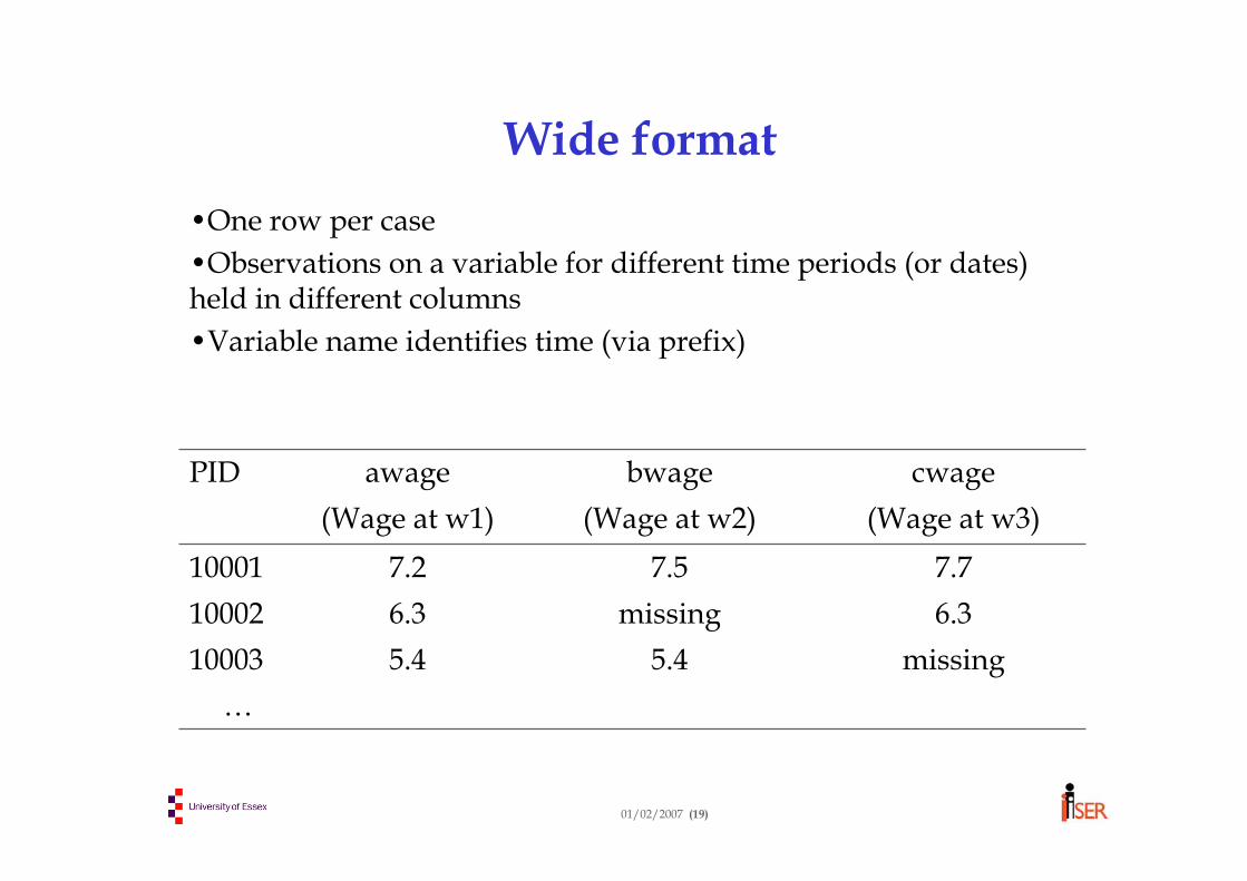
Wide format•One row per case •Observations on a variable for different time periods (or dates)held in different columns •Variable name identifies time (via prefix)

…missing5.45.410003

6.3missing6.3100027.77.57.210001

(Wage at w3)(Wage at w2)(Wage at w1)cwagebwageawagePID

01/02/2007 (20)

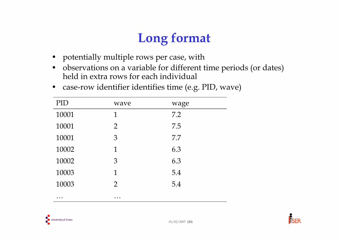
Long format• potentially multiple rows per case, with • observations on a variable for different time periods (or dates)

held in extra rows for each individual • case-row identifier identifies time (e.g. PID, wave)

……5.42100035.41100036.33100026.31100027.73100017.52100017.2110001wage wavePID

01/02/2007 (21)

Matching (or merging)• Joining two (or more) files at the same level of observation (e.g.

person files) where both (all) files contain the same identifiervariable used as key

• 1:1 matching – one case in “master file” corresponds to one case in “using file” (i.e. the file being matched in)

• 1:many – one case in the “using file” may be ‘distributed’ to many cases in the “master file”• E.g. info. about a household attached to each one of the household’s

members• In either case, not all cases in master file may receive match; not

all cases in the using file may provide a match• Stata’s command: merge key using file

• Merging is the source of many disastrous errors – always check by using tabulate _merge (see examples later)

01/02/2007 (22)

Aggregation• Deriving group-level information from all the

members of that group• E.g. calculating household income from the incomes of its

members• E.g. calculating how many children a woman has during her

first marriage• The group-level information may be used in two

ways: • (i) saved in a new file with the group – e.g. household or

spell – as the case (collapse)• (ii) attributed to each of the group members within the

existing file (egen; by(sort): …)

01/02/2007 (23)

Appending• Combining files with no index-based matching

• E.g. combining file A with n1 rows and file B with n2 rows to produce a new file C with n1+n2 rows.

• Stata command: append• Used to assemble a sequence of annual cross-section

data files into a single long-format panel data file• Rows in new combined files are specific to a person-wave

combination• Each variable must have the same name in each of

the annual cross-section files

01/02/2007 (24)

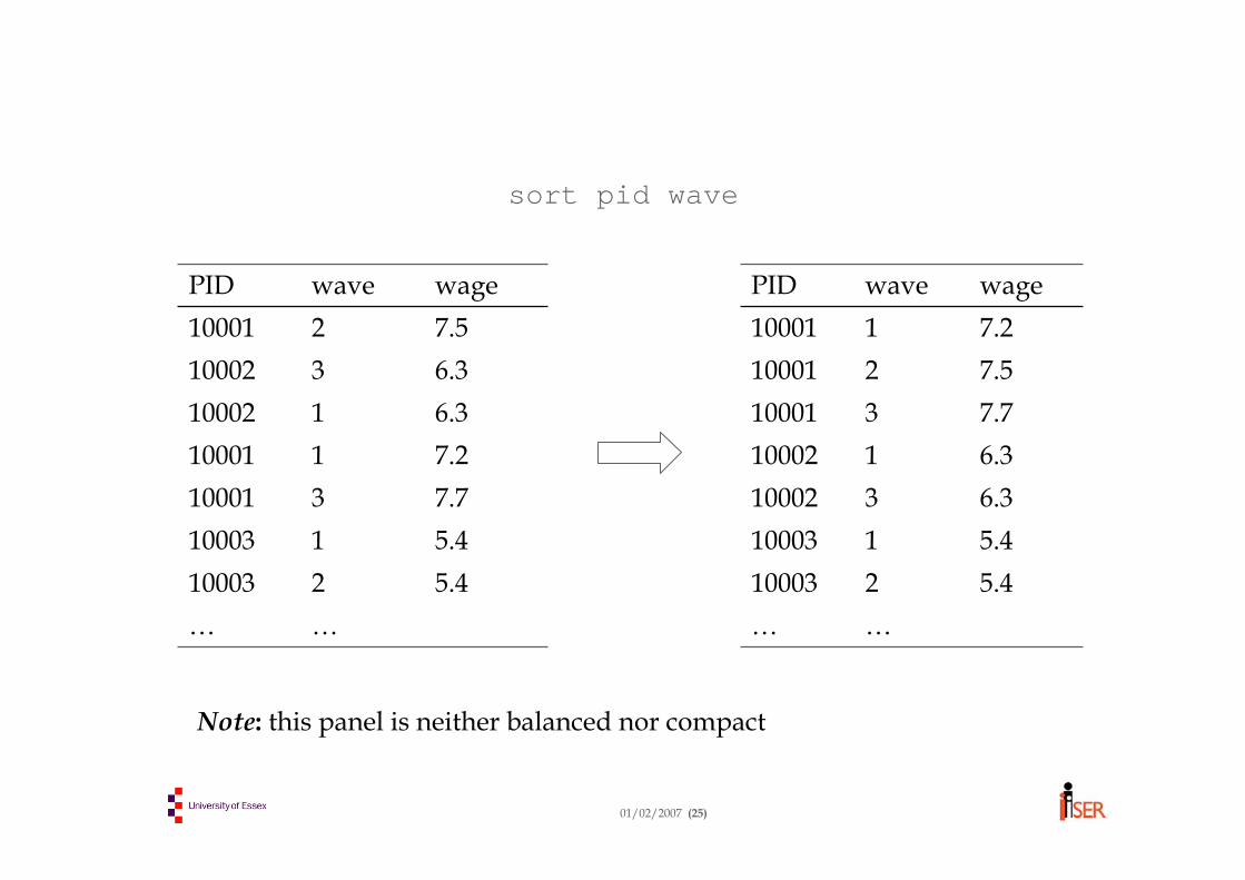
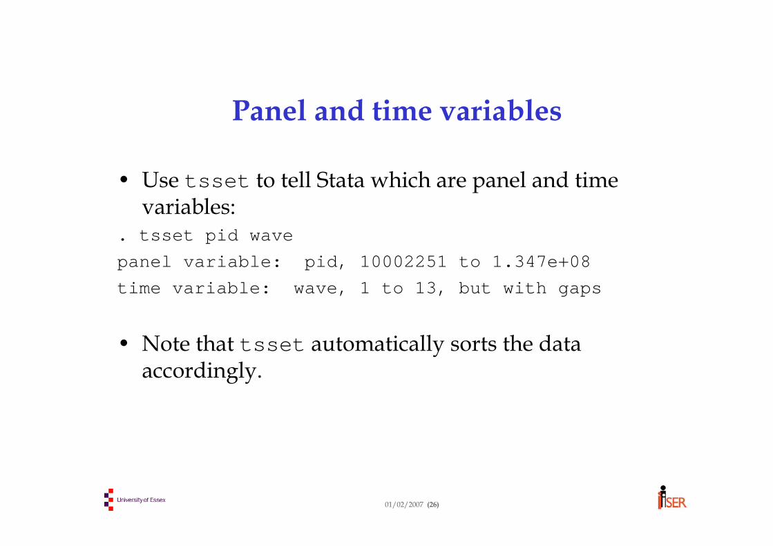
Sorting (ordering) the data

• We now have a dataset in long format• It’s a good idea to order the data for easier viewing.

“Eyeballing” the data is important!• We also have to tell Stata which variable identifies

the individual (Stata calls this the panel variable).• We may also have to tell Stata which variable

identifies the repeated observation (Stata calls this the time variable).

For some types of panel analysis we don’t need to know the ordering of the repeated observations

01/02/2007 (25)

7.52100016.33100026.3110002

7.7310001

……5.42100035.4110003

7.2110001

wage wavePID

……5.42100035.41100036.33100026.31100027.73100017.52100017.2110001wage wavePID

sort pid wave

Note: this panel is neither balanced nor compact

01/02/2007 (26)

Panel and time variables

• Use tsset to tell Stata which are panel and time variables:

. tsset pid wavepanel variable: pid, 10002251 to 1.347e+08time variable: wave, 1 to 13, but with gaps

• Note that tsset automatically sorts the data accordingly.

01/02/2007 (27)

Describing panel data• Ways of describing/summarising panel data:

Basic patterns of available casesBetween- and within-group components of variationTransition tables

• Some basic notation:yit is the “dependent variable” to be analysed

i indexes the individual (pid), i = 1, 2, …, nt indexes the repeated observation / time period (wave), t = 1, 2, …, Ti

• yit may be: continuous (e.g. wages); mixed discrete/continuous (e.g. hours of work); binary (e.g. employed/not employed); ordered discrete (e.g. Likert scale for degree of happiness); unordered discrete (e.g. occupation)

01/02/2007 (28)

Describe patterns of panel data: xtdes. xtdes

pid: 10002251, 10004491, ..., 1.347e+08 n = 16082wave: 1, 2, ..., 13 T = 13

Delta(wave) = 1; (13-1)+1 = 13(pid*wave uniquely identifies each observation)

Distribution of T_i: min 5% 25% 50% 75% 95% max1 1 2 7 13 13 13

Freq. Percent Cum. | Pattern---------------------------+---------------

4648 28.90 28.90 | 1111111111111997 6.20 35.10 | 1............646 4.02 39.12 | 11...........376 2.34 41.46 | ............1342 2.13 43.58 | 111..........327 2.03 45.62 | 1111.........261 1.62 47.24 | ...........11254 1.58 48.82 | .1...........251 1.56 50.38 | ..........1117980 49.62 100.00 | (other patterns)

---------------------------+---------------16082 100.00 | XXXXXXXXXXXXX

01/02/2007 (29)

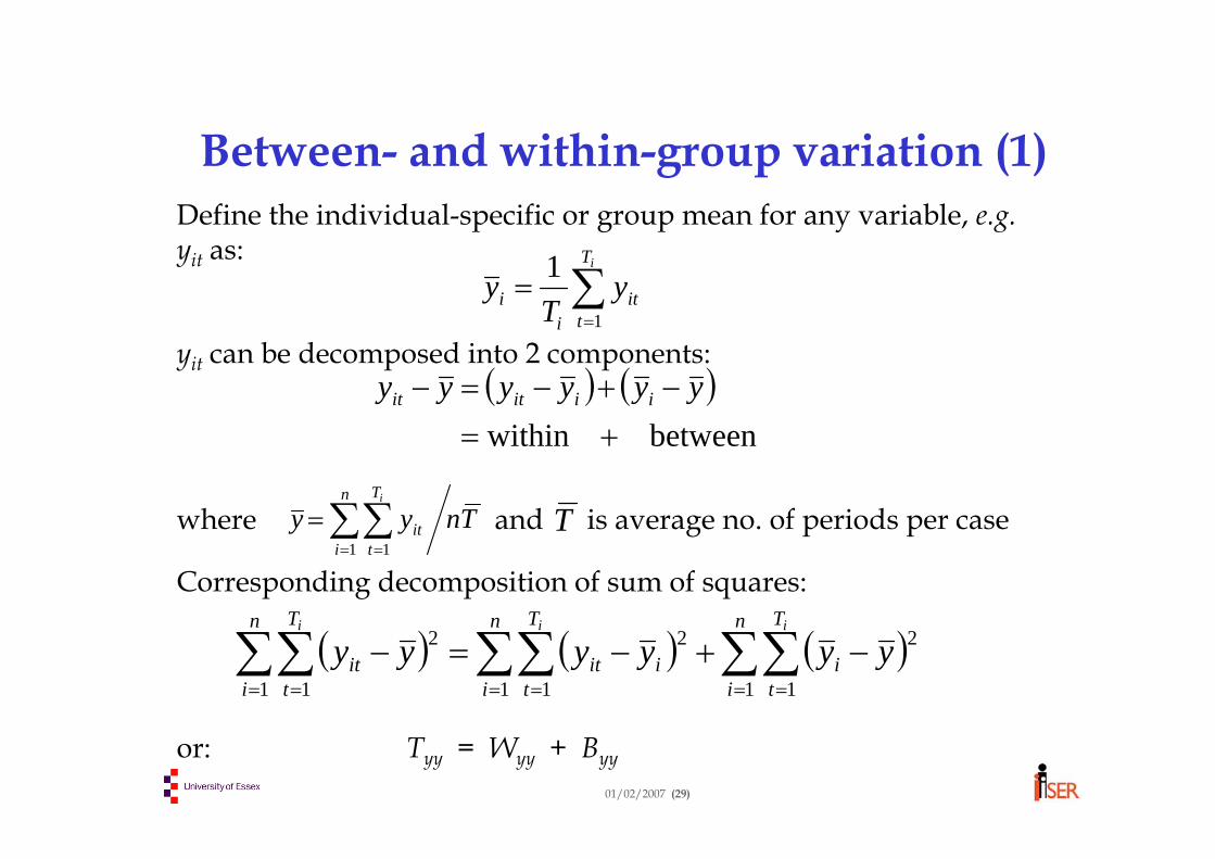
Between- and within-group variation (1)Define the individual-specific or group mean for any variable, e.g.yit as:

yit can be decomposed into 2 components:

where and is average no. of periods per case

Corresponding decomposition of sum of squares:

or: Tyy = Wyy + Byy

∑=

=iT

tit

ii y

Ty

1

1

( ) ( )betweenwithin +=−+−=− yyyyyy iiitit

( ) ( ) ( )∑∑∑∑∑∑= == == =

−+−=−n

i

T

ti

n

i

T

tiit

n

i

T

tit

iii

yyyyyy1 1

2

1 1

2

1 1

2

Tnyyn

i

T

tit

i

∑∑= =

=1 1

T

01/02/2007 (30)

Between- and within-group variation (2)• Between and within variation is the basis of linear

panel regression. Important concept to understand.• Simple example: balanced panel (n=1119, T = 13) of

workers who have reported their wages.• From summarize, we have grand mean wage ( ) =

£9.84 per hour, and (overall) variance of wages = 32.63. Recall the standard formula for variance:

y

( )

111 1

2

2

−≡

−

−=∑∑= =

TnT

Tn

yys yy

n

i

T

tit

01/02/2007 (31)

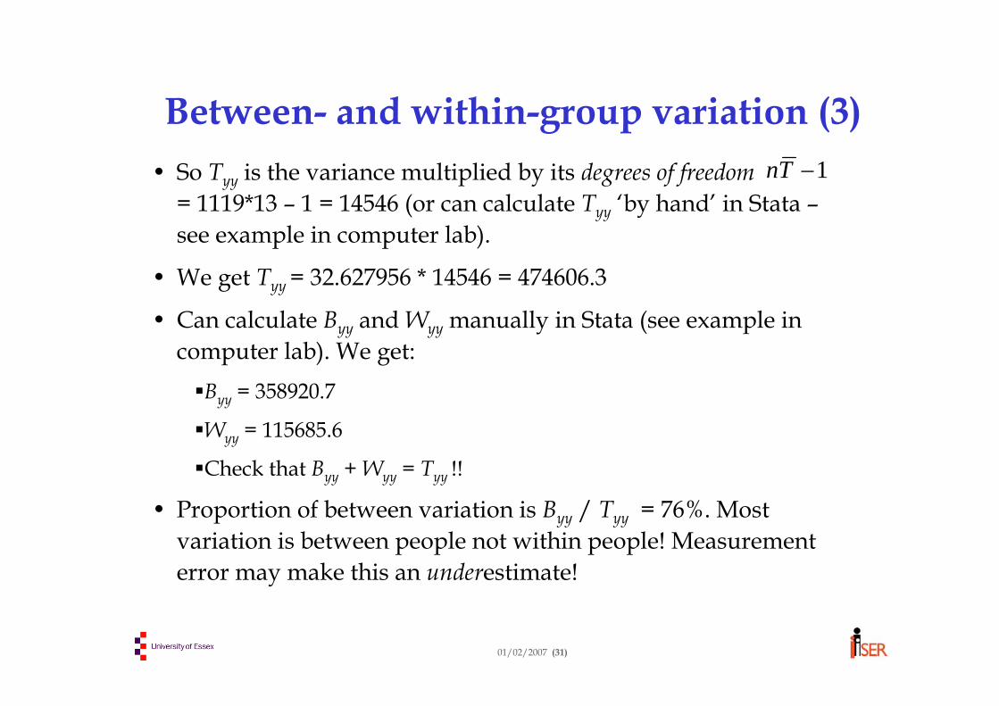
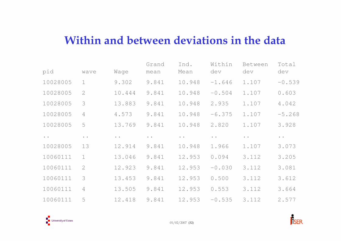
Between- and within-group variation (3)• So Tyy is the variance multiplied by its degrees of freedom

= 1119*13 – 1 = 14546 (or can calculate Tyy ‘by hand’ in Stata –see example in computer lab).

• We get Tyy = 32.627956 * 14546 = 474606.3

• Can calculate Byy and Wyy manually in Stata (see example in computer lab). We get:

Byy = 358920.7

Wyy = 115685.6

Check that Byy + Wyy = Tyy !!

• Proportion of between variation is Byy / Tyy = 76%. Most variation is between people not within people! Measurement error may make this an underestimate!

1−Tn

01/02/2007 (32)

Within and between deviations in the data

2.5773.112-0.53512.9539.84112.418510060111

3.6643.1120.55312.9539.84113.505410060111

3.6123.1120.50012.9539.84113.453310060111

3.0813.112-0.03012.9539.84112.923210060111

3.2053.1120.09412.9539.84113.046110060111

3.0731.1071.96610.9489.84112.9141310028005

................

3.9281.1072.82010.9489.84113.769510028005

-5.2681.107-6.37510.9489.8414.573410028005

4.0421.1072.93510.9489.84113.883310028005

0.6031.107-0.50410.9489.84110.444210028005

-0.5391.107-1.64610.9489.8419.302110028005

Total dev

Between dev

Within dev

Ind. Mean

Grand meanWagewavepid

01/02/2007 (33)

Between- and within-group variation: xtsum

• Stata contains a ‘canned’ routine, xtsum, that summarises within and between variation.

• Doesn’t give an exact decomposition:Converts sums of squares to variance using different ‘degrees offreedom’ so they are not comparableReports square root (i.e. standard deviation) of these variancesDocumentation is not very clear!

. xtsum wage

Variable | Mean Std. Dev. Min Max | Obs--------------+----------------------------------------+----------wage overall | 9.841044 5.712089 .3813552 121.7474 | N = 14547

between | 4.969431 3.322259 46.54612 | n = 1119within | 2.820121 -18.37394 108.5192 | T = 13

01/02/2007 (34)

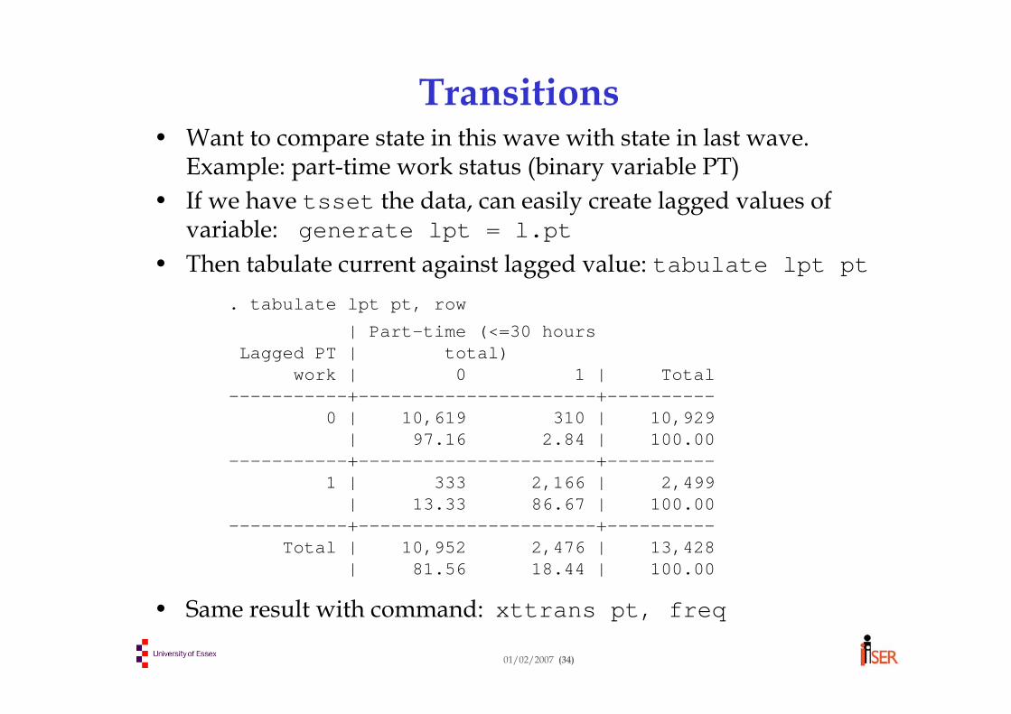
Transitions • Want to compare state in this wave with state in last wave.

Example: part-time work status (binary variable PT)• If we have tsset the data, can easily create lagged values of

variable: generate lpt = l.pt• Then tabulate current against lagged value: tabulate lpt pt

• Same result with command: xttrans pt, freq

. tabulate lpt pt, row

| Part-time (<=30 hoursLagged PT | total)

work | 0 1 | Total-----------+----------------------+----------

0 | 10,619 310 | 10,929 | 97.16 2.84 | 100.00

-----------+----------------------+----------1 | 333 2,166 | 2,499 | 13.33 86.67 | 100.00

-----------+----------------------+----------Total | 10,952 2,476 | 13,428

| 81.56 18.44 | 100.00

01/02/2007 (35)

Transitions and measurement error

. tab d1evec if wave==1

have you ever taken |cannabis | Freq. Percent Cum.

---------------------+-----------------------------------yes | 855 25.45 25.45

no | 2,477 73.72 99.17don't know | 13 0.39 99.55

don't want to answer | 15 0.45 100.00

---------------------+-----------------------------------Total | 3,360 100.00

Analysis of transitions can give good indications of data (un)reliability

Example: UK Offending Crime & Justice Survey (2003-4, ages 10-25)

01/02/2007 (36)

Transition matrix. xttrans d1evec, freq

have you |ever taken | have you ever taken cannabis

cannabis | Yes No DK DWTA | Total-----------+--------------------------------------------+----------

Yes | 728 111 0 1 | 840 | 86.67 13.21 0.00 0.12 | 100.00

-----------+--------------------------------------------+----------No | 251 2,189 6 7 | 2,453

| 10.23 89.24 0.24 0.29 | 100.00 -----------+--------------------------------------------+----------

DK | 2 9 1 1 | 13 | 15.38 69.23 7.69 7.69 | 100.00

-----------+--------------------------------------------+----------DWTA | 9 5 0 1 | 15

| 60.00 33.33 0.00 6.67 | 100.00 -----------+--------------------------------------------+----------

Total | 990 2,314 7 10 | 3,321 | 29.81 69.68 0.21 0.30 | 100.00

• 13% of people who’d used cannabis before 2003 say they’ve never used before 2004!!

01/02/2007 (37)

Age and cohort: earnings profiles

68

1012

20 30 40 50 60ageseq

profile39 profile4044profile4549 profile5054profile5559 profile6064profile6569 profile7074profile75

How have different generations fared in the labour market?

01/02/2007 (1)

Day 2:

Approaches to modelling

01/02/2007 (2)

Basic notation

We work with observed variables yit , zi and xit :

yit = dependent variable to be analysed

zi = time-invariant characteristics (e.g. year of birth, sex)

xit = time-varying characteristics (e.g. job tenure, marital status)

where i indexes individuals, t indexes time periods.

01/02/2007 (3)

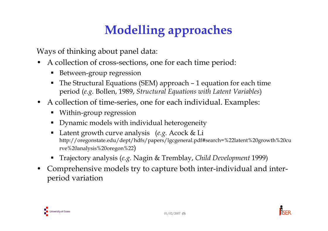
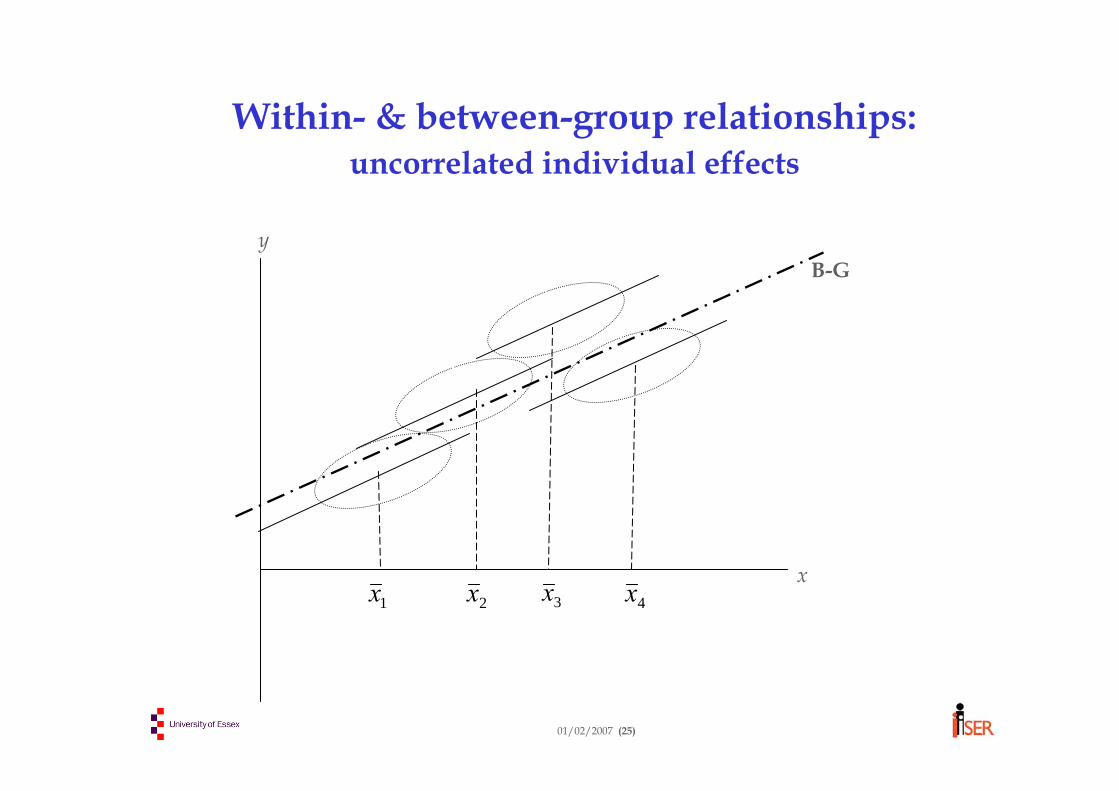
Modelling approaches Ways of thinking about panel data:• A collection of cross-sections, one for each time period:

Between-group regressionThe Structural Equations (SEM) approach – 1 equation for each time period (e.g. Bollen, 1989, Structural Equations with Latent Variables)

• A collection of time-series, one for each individual. Examples:Within-group regressionDynamic models with individual heterogeneityLatent growth curve analysis (e.g. Acock & Li http://oregonstate.edu/dept/hdfs/papers/lgcgeneral.pdf#search=%22latent%20growth%20curve%20analysis%20oregon%22)Trajectory analysis (e.g. Nagin & Tremblay, Child Development 1999)

• Comprehensive models try to capture both inter-individual and inter-period variation

01/02/2007 (4)

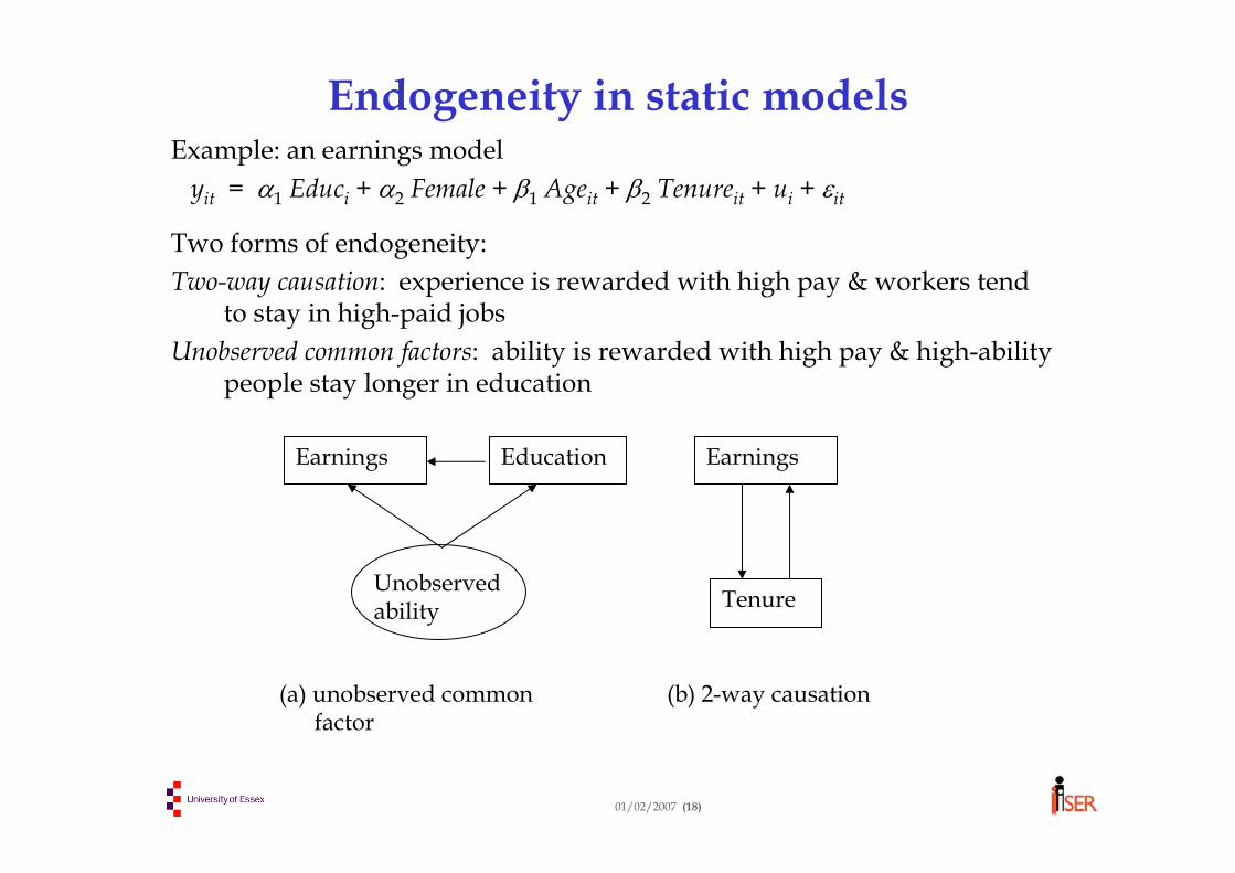
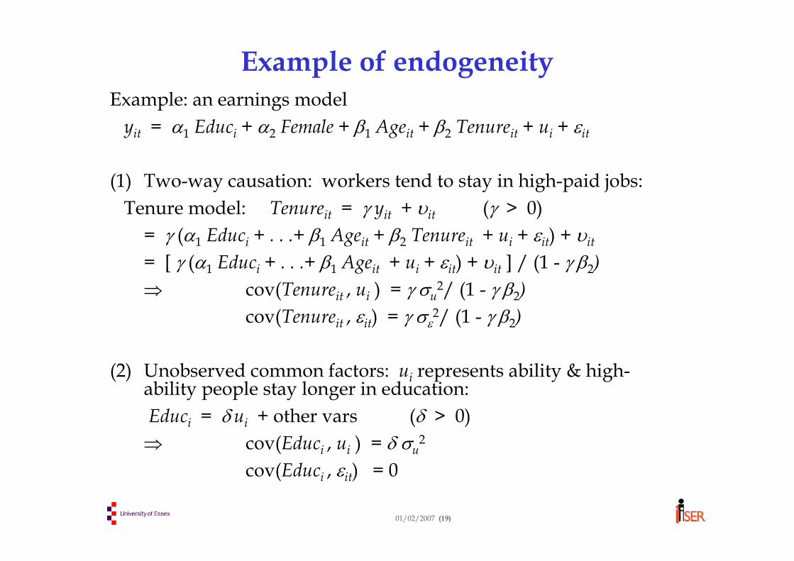
Why use panel data?The disadvantages of cross-section data

Example: cross-section earnings regression (single time period, t subscript suppressed)

yi = ziα + xi β + εi

where:yi = log wage; zi = observable time-invariant factors (education, etc.); xi = observable time-varying factors (e.g. job tenure); εi = random error (e.g. “luck”)

Possible misspecifications, causing bias:• Omitted dynamics (lagged variables not observed)• Reverse causation (e.g. pay and tenure jointly determined) • Omitted unobservables (e.g. “ability”)

01/02/2007 (5)

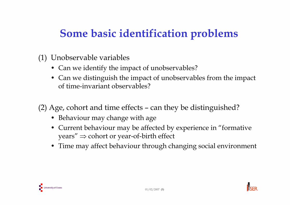
Some basic identification problems

(1) Unobservable variables• Can we identify the impact of unobservables? • Can we distinguish the impact of unobservables from the impact

of time-invariant observables?

(2) Age, cohort and time effects – can they be distinguished?• Behaviour may change with age• Current behaviour may be affected by experience in “formative

years” ⇒ cohort or year-of-birth effect• Time may affect behaviour through changing social environment

01/02/2007 (6)

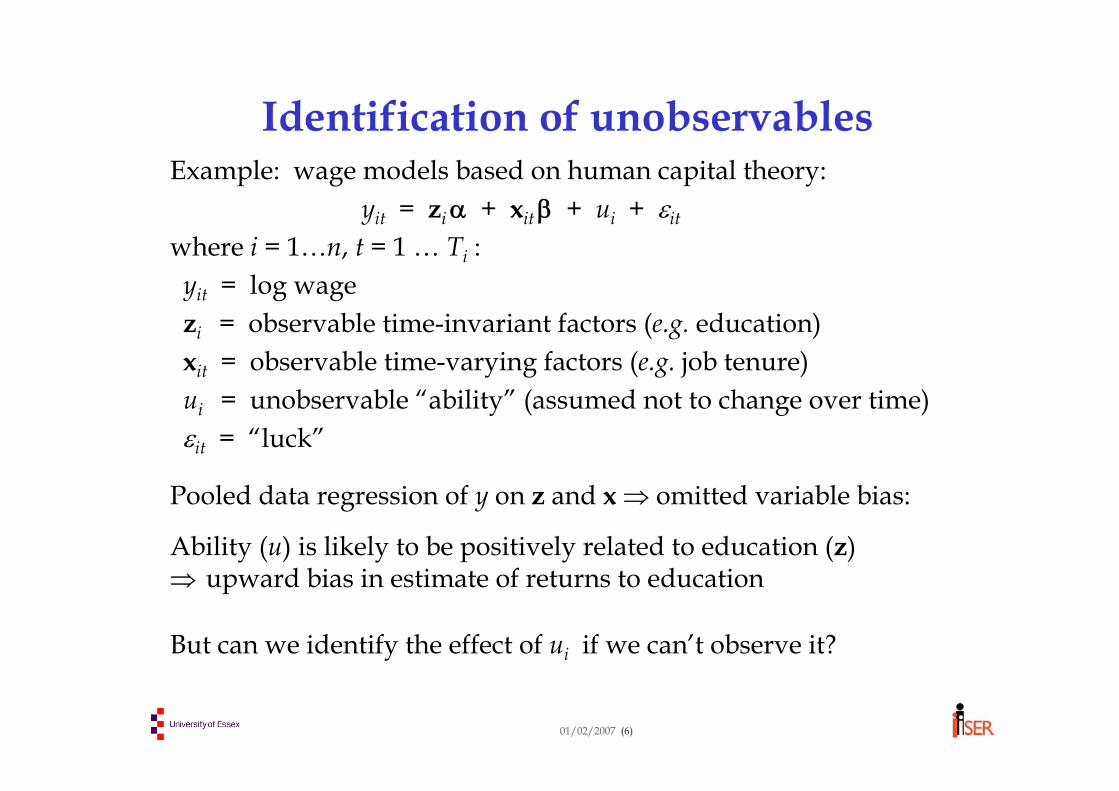
Identification of unobservablesExample: wage models based on human capital theory:

yit = ziα + xitβ + ui + εit

where i = 1…n, t = 1 … Ti :yit = log wagezi = observable time-invariant factors (e.g. education)xit = observable time-varying factors (e.g. job tenure)ui = unobservable “ability” (assumed not to change over time)εit = “luck”

Pooled data regression of y on z and x ⇒ omitted variable bias:

Ability (u) is likely to be positively related to education (z) ⇒ upward bias in estimate of returns to education

But can we identify the effect of ui if we can’t observe it?

01/02/2007 (7)

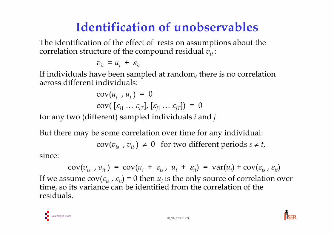
Identification of unobservablesThe identification of the effect of rests on assumptions about the correlation structure of the compound residual vit :

vit = ui + εit

If individuals have been sampled at random, there is no correlation across different individuals:

cov(ui , uj ) = 0cov( [εi1 … εiT], [εj1 … εjT]) = 0

for any two (different) sampled individuals i and j

But there may be some correlation over time for any individual:cov(vis , vit ) ≠ 0 for two different periods s ≠ t,

since: cov(vis , vit ) = cov(ui + εis , ui + εit) = var(ui) + cov(εis , εit)

If we assume cov(εis , εit) = 0 then ui is the only source of correlation over time, so its variance can be identified from the correlation of the residuals.

01/02/2007 (8)

Identification with time-invariant covariates: can we distinguish zi and ui?

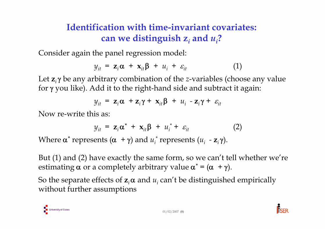
Consider again the panel regression model:

yit = ziα + xitβ + ui + εit (1)Let zi γ be any arbitrary combination of the z-variables (choose any value for γ you like). Add it to the right-hand side and subtract it again:

yit = ziα + zi γ + xitβ + ui - zi γ + εit

Now re-write this as:yit = ziα* + xitβ + ui

* + εit (2)Where α* represents (α + γ) and ui

* represents (ui - zi γ).

But (1) and (2) have exactly the same form, so we can’t tell whether we’re estimating α or a completely arbitrary value α* = (α + γ).So the separate effects of ziα and ui can’t be distinguished empirically without further assumptions

01/02/2007 (9)

SummaryIn models like:

yit = ziα + xit β + ui + εit

• We can only identify the effect of unobservable ability ui if we can assume that εit is serially-independent (or some other simple autocorrelation structure).

• We cannot distinguish the separate effects of zi and uiwithout making further assumptions (e.g. no correlation between zi and ui).

01/02/2007 (10)

Identification problem (2): Age, cohort & time effects

Fundamental identity relating age (Ait), time of interview (t) and birth cohort (Bi):

Ait ≡ t –BiThese three cannot be distinguished in principle. To do so

would require an ability to move a cohort forward or back in time (!) to measure the effect of time holding age and cohort constant.

• In a cross-section, t doesn’t vary, so time effects can’t be estimated and age or cohort are collinear – only their joint effect can be estimated

• In a panel, t varies but Ait , t and Bi are collinear - only two of the three effects can be estimated.

• So we can use (t ,Bi) , (Ait ,Bi) or (Ait ,t) as covariates, but not all three.

01/02/2007 (11)

Age, cohort and time effects

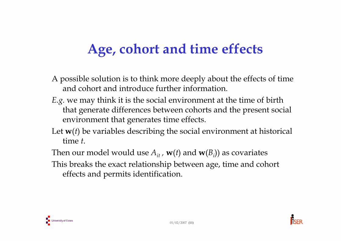
A possible solution is to think more deeply about the effects of time and cohort and introduce further information.

E.g. we may think it is the social environment at the time of birth that generate differences between cohorts and the present socialenvironment that generates time effects.

Let w(t) be variables describing the social environment at historical time t.

Then our model would use Ait , w(t) and w(Bi)) as covariatesThis breaks the exact relationship between age, time and cohort

effects and permits identification.

01/02/2007 (12)

When to use regression methodsRegression models are suitable for the analysis of dependent variables yit which can vary continuously, so:

Income, birthweight, etc. ⇒ regression appropriateAge at retirement, interpolated grouped income, etc. ⇒ regression may work OKAge of school leaving, no. of visits to doctor last week, etc. ⇒regression a bit riskyBinary variables (married/non-married, employed/non-employed, etc. ⇒ regression very unreliable

Regression models also have technical problems when:The sample is censored or truncated (e.g. if yit = hours of work and non-workers are recorded as zero or excluded)When there is no natural scale (e.g. Likert scales)

01/02/2007 (13)

Related methods (1)Latent growth curve analysis is widely used in sociology, psychology, criminology, etc. but not economics

Example: simple quadratic latent growth curve:yit = ui + αi t + βi t2 + εit

where the intercept and slope coefficients (ui , αi , βi) vary randomly across individualsAdvantage:

Doesn’t assume all individuals have the same coefficients (panel data regression assumes no variation in αi , βi )

Disadvantage:Purely descriptive: no theory of developmentCrude dynamics (nothing changes the trend for an individual once it’s underway)

01/02/2007 (14)

Related methods (2)Structural equation modelling (SEM) is widely used in psychology and economics, but with differences in terminology.

In panel data applications, each year is described by a different equation:

Period 1: yi1 = ziα1 + xi1 β1 + ui + εi1..

Period T: yiT = ziαT + xiT βT + ui + εiT

Advantage:general structure (e.g. panel regression is special case where the αt and βtare the same in all periods)

Disadvatage:No theory of how the parameters vary over timeCan’t predict outcomes in new periodsDifficult to use in long or very unbalanced panels

01/02/2007 (15)

Related methods (3)Multi-level modelling is widely used throughout social statistics. It generalises ordinary panel data applications to multiple dimensionsExample: time periods (t) within individuals (i) within households (h):

yhit = xhit β + uhi + wh + εiTwh is the household effect, common to all individuals at all periods within household huhi is the individual effect, common to all time periods for the ithindividual in household h

Specialist software is available for latent growth curve, SEM and Multi-level analysis (MLwin, Mplus, LISREL, etc). See also xtmixed and GLLAMM in Stata

01/02/2007 (16)

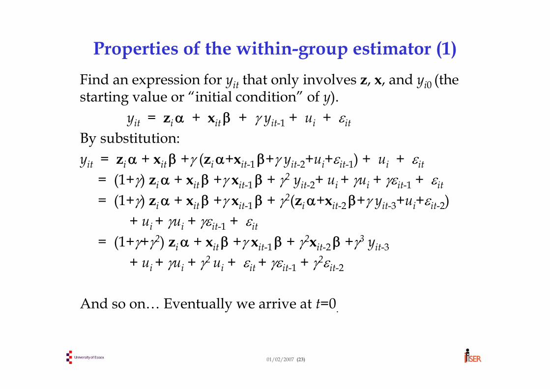
Pooled regression for panel dataThe “standard” panel data regression model is:


We have observations indexed by t = 1 … Ti , i = 1 … n.• A pooled regression of y on z and x using all the data together

would assume that there is no correlation across individuals, nor across time periods for any individual

• This would ignore the individual effect u, which generates correlation between the values of (ui + εi1) … (ui + εiT) for each individual i

• So pooled regression doesn’t make best use of the dataUnder favourable conditions (if ui is uncorrelated with zi and xit ), pooled regression gives unbiased but inefficient results, with incorrect standard errors, t-ratios, etc.If ui is correlated with zi and xit , pooled regression is also biased

01/02/2007 (17)

Least-squares dummy variable (LSDV) regression

The panel data regression model is:


We have observations indexed by t = 1 … Ti , i = 1 … n.The ui can be captured using dummy variables. Construct a set of ndummy variables D1i … Dni , where:

Dri = 1 if i = r and 0 otherwise, for r = 1 … nThus Drit tells us whether observation i, t relates to person r.The model is now:

yit = ziα + xitβ + u1 D1i + … + unDni + εit

So u1 … un are now seen as the coefficients of a set of n dummy variables.

01/02/2007 (18)

Shortcut calculation of the LSDVregressionA multiple regression of y on (z , x) and (D1 … Dn) can be done in

two stages:Stage 1: Eliminate the effect of (D1 … Dn) on each of the variables

(y, z , x) using the “within-group” data transformation:

(so zi is eliminated completely)

Stage 2: regress y* on (z* , x*) : in other words, on [Intuition: think of regressing a variable on a constant. Estimate of constant is mean and residual is deviation from mean.]

This is exactly equivalent to regressing y on (z , x) and (D1 … Dn)

iit yy −

0zzz

xxx

≡−=

−=

−=

iii

iitit

iitit yyy

*

*

*

iit xx −

01/02/2007 (19)

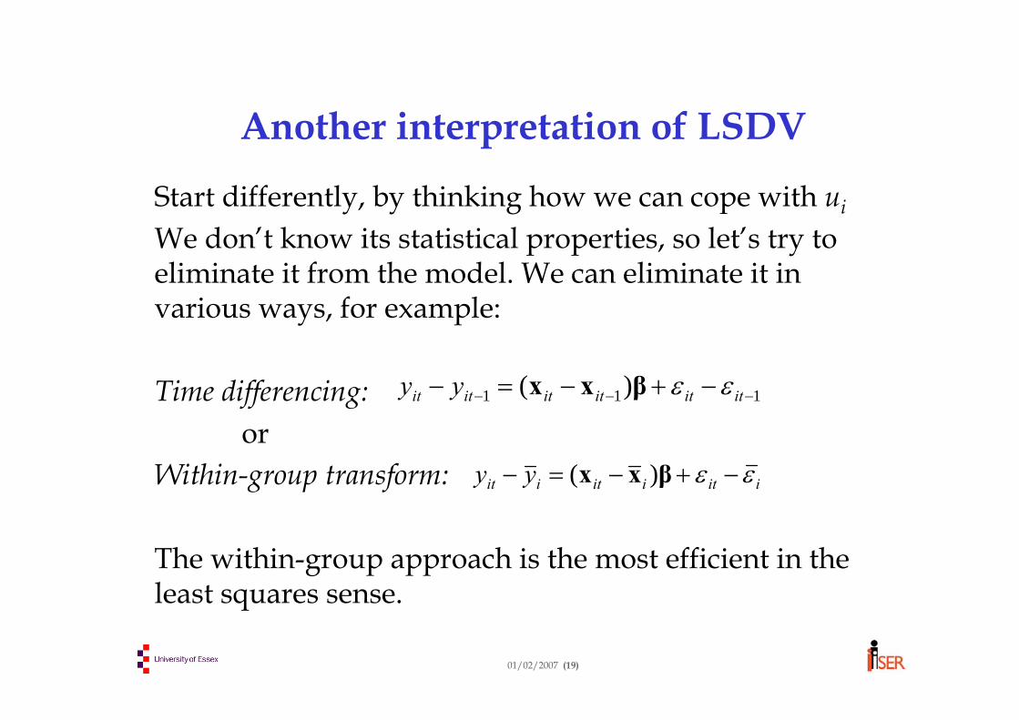
Another interpretation of LSDV

Start differently, by thinking how we can cope with ui

We don’t know its statistical properties, so let’s try to eliminate it from the model. We can eliminate it in various ways, for example:

Time differencing:or

Within-group transform:

The within-group approach is the most efficient in the least squares sense.

111 )( −−− −+−=− itititititit yy εεβxx

iitiitiit yy εε −+−=− βxx )(

01/02/2007 (20)

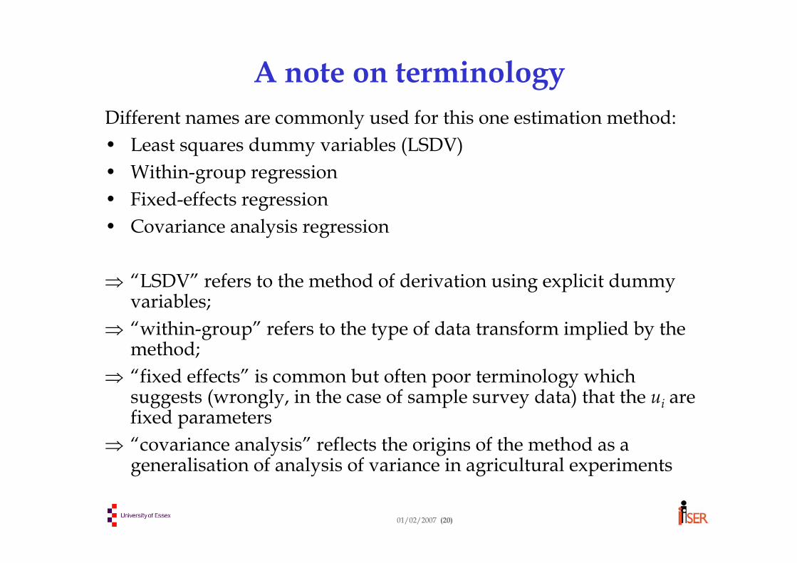
A note on terminologyDifferent names are commonly used for this one estimation method:• Least squares dummy variables (LSDV)• Within-group regression• Fixed-effects regression• Covariance analysis regression

⇒ “LSDV” refers to the method of derivation using explicit dummy variables;

⇒ “within-group” refers to the type of data transform implied by the method;

⇒ “fixed effects” is common but often poor terminology which suggests (wrongly, in the case of sample survey data) that the ui are fixed parameters

⇒ “covariance analysis” reflects the origins of the method as a generalisation of analysis of variance in agricultural experiments

01/02/2007 (21)

Between-group regressionInstead of eliminating ui from the regression, we can amplify it by averaging out all the within-individual variation, leaving only between-individual variation to analyse:Between-group transform:

Then regress on in one of two ways:Use one group-mean observation per individualUse Ti copies of the group mean data for individual i

Note: The latter is equivalent to a weighted regression of on , with a weight of Ti for individual i. It is often desirable to give more weight to individuals with many time observations.

iy

iiiii uy ε+++= βxαz

( )ii xz ,

iy ix

01/02/2007 (22)

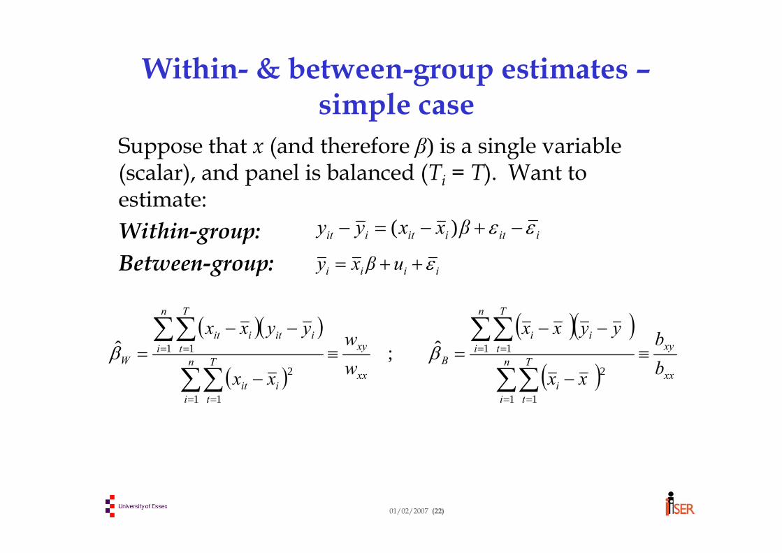
Within- & between-group estimates –simple case

Suppose that x (and therefore β) is a single variable (scalar), and panel is balanced (Ti = T). Want to estimate: Within-group:Between-group:

iitiitiit βxxyy εε −+−=− )(

( )( )

( )

( )( )

( ) xx

xyn

i

T

ti

n

i

T

tii

Bxx

xyn

i

T

tiit

n

i

T

tiitiit

W bb

xx

yyxx

ww

xx

yyxx≡

−

−−=≡

−

−−=

∑∑

∑∑

∑∑

∑∑

= =

= =

= =

= =

1 1

2

1 1

1 1

2

1 1 ˆ;ˆ ββ

iiii uβxy ε++=

01/02/2007 (23)

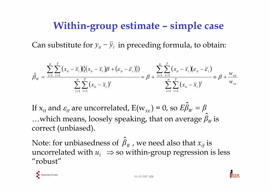
Within-group estimate – simple case

Can substitute for in preceding formula, to obtain:

If xit and εit are uncorrelated, E(wxε ) = 0, so …which means, loosely speaking, that on average is correct (unbiased).

Note: for unbiasedness of , we need also that xit is uncorrelated with ui ⇒ so within-group regression is less “robust”

iit yy −

( ) ( ) ( ) ( )

( )

( )( )

( ) xx

xn

i

T

tiit

n

i

T

tiitiit

n

i

T

tiit

n

i

T

tiitiitiit

W ww

xx

xx

xx

xxxxεβ

εεβ

εεββ +≡

−

−−+=

−

−+−−=

∑∑

∑∑

∑∑

∑∑

= =

= =

= =

= =

1 1

2

1 1

1 1

2

1 1ˆ

ββE W =ˆ

Wβ

Bβ

01/02/2007 (24)

Within- & between-group relationships:correlated individual effects

1x 3x2x 4xx

y

B-G

W-G

W-G

W-GW-G

u1

u2

u3

In this example, individual effects are negatively correlated with , so B-G & W-G relationships differix

01/02/2007 (25)

Within- & between-group relationships:uncorrelated individual effects

1x 3x2x 4xx

yB-G

01/02/2007 (26)

Example of panel data estimation

The Stata command xtreg computes within-group and between-group regressions

Example: within- and between-group regressions of log earnings on age, year of birth and time, allowing for unobserved individual effects:

gen age=year-cohortgen lwage=ln(w_hr)xtreg lwage age cohort, fextreg lwage age cohort, be

01/02/2007 (27)

Stata output: within-group regression. xtreg lwage age cohort , fe

Fixed-effects (within) regression Number of obs = 61516Group variable (i): pid Number of groups = 10335

R-sq: within = 0.1217 Obs per group: min = 1between = 0.0312 avg = 6.0overall = 0.0194 max = 14

F(1,51180) = 7094.59corr(u_i, Xb) = -0.4880 Prob > F = 0.0000

------------------------------------------------------------------------------lwage | Coef. Std. Err. t P>|t| [95% Conf. Interval]

-------------+----------------------------------------------------------------age | .030061 .0003569 84.23 0.000 .0293615 .0307605

cohort | (dropped)_cons | .8994719 .01369 65.70 0.000 .8726394 .9263045

-------------+----------------------------------------------------------------sigma_u | .60455798sigma_e | .28494801

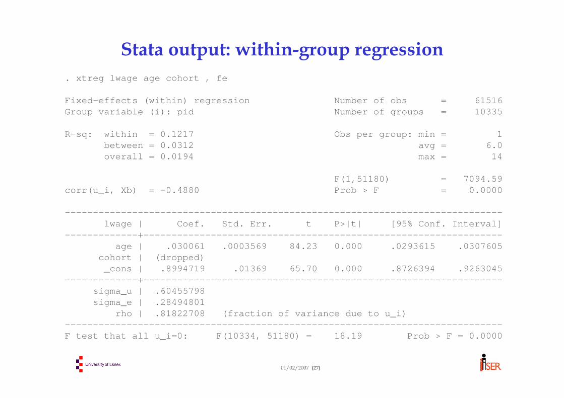
rho | .81822708 (fraction of variance due to u_i)------------------------------------------------------------------------------F test that all u_i=0: F(10334, 51180) = 18.19 Prob > F = 0.0000

01/02/2007 (28)

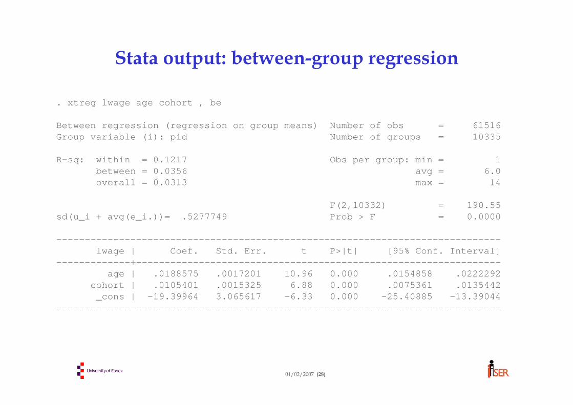
Stata output: between-group regression

. xtreg lwage age cohort , be

Between regression (regression on group means) Number of obs = 61516Group variable (i): pid Number of groups = 10335


F(2,10332) = 190.55sd(u_i + avg(e_i.))= .5277749 Prob > F = 0.0000


-------------+----------------------------------------------------------------age | .0188575 .0017201 10.96 0.000 .0154858 .0222292

cohort | .0105401 .0015325 6.88 0.000 .0075361 .0135442_cons | -19.39964 3.065617 -6.33 0.000 -25.40885 -13.39044

------------------------------------------------------------------------------

01/02/2007 (29)

Important points

• The within-group R2 is much higher than the between-group R2

⇒ the covariate age “explains” a reasonable amount of the pay variation over time for a given individual ⇒ but pay differences between individuals are lessclosely related to age and cohort in R2 terms

• The large coefficient differences between the within-and between-group age coefficients suggest that a single regression model with classical assumptions doesn’t fit the evidence very well

01/02/2007 (30)

Technical appendix

The following slides can be safely ignored if you’re not interested in technical detail or if you aren’t familiar with vector-matrix notation and matrix algebra

01/02/2007 (31)

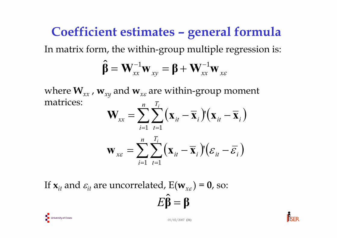
Coefficient estimates – general formulaIn matrix form, the within-group multiple regression is:

where Wxx , wxy and wxε are within-group moment matrices:

If xit and εit are uncorrelated, E(wxε ) = 0, so:

εxxxxyxx wWβwWβ 11ˆ −− +==

( ) ( )

( ) ( )∑∑

∑∑

= =

= =

−−=

−−=

n

i

T

tiitiitx

n

i

T

tiitiitxx

i

i

1 1

1 1

'

'

εεε xxw

xxxxW

ββ =ˆE

01/02/2007 (32)

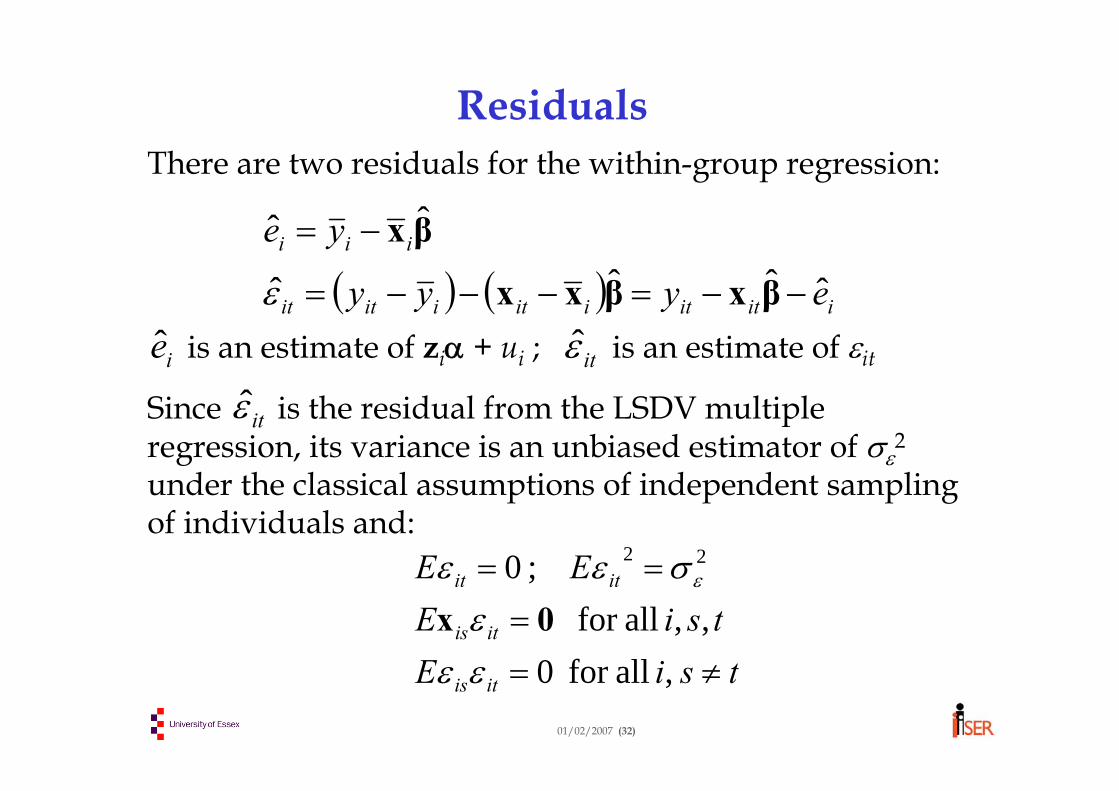
ResidualsThere are two residuals for the within-group regression:

is an estimate of ziα + ui ; is an estimate of εit

Since is the residual from the LSDV multiple regression, its variance is an unbiased estimator of σε

2

under the classical assumptions of independent sampling of individuals and:

( ) ( ) iititiitiitit

iii

eyyy

ye

ˆˆˆˆ

ˆˆ

−−=−−−=

−=

βxβxx

βx

ε

ie itε

itε

tsiEtsiE

EE

itis

itis

itit

≠==

==

, allfor 0,, allfor

;0 22

εεε

σεε ε

0x

01/02/2007 (33)

Estimation of αThe residual can be written:

Since is an estimate of ziα + ui , we could regress it on zi to estimate α. (Use Ti repeated observations on the group means for individual i, to weight individuals appropriately). This gives:

where Bxx etc. are between-group cross-product matrices:

ie

ie

ezzz ˆ1ˆ bBα −=

( )( )ββxαz

βxβxαzβx

−−++=

−+++=−=ˆ

ˆˆˆ

iiii

iiiiiiii

u

uye

ε

ε

∑∑∑∑= == =

==n

i

T

tiiez

n

i

T

tiizz

ii

e1 1

ˆ1 1

ˆ';' zbzzB

01/02/2007 (34)

Estimation of

Rewrite as:

But is unbiased and we assume zi is uncorrelated with εit , so:

Thus is only unbiased if ui and zi are uncorrelated.

( )ββBBbBbBαbBα −−++== −−−− ˆˆ 111ˆ

1zxzzzzzzuzzezzz ε

β

( )zuzzEE bBαα 1ˆ −+=

α

α

α

01/02/2007 (35)

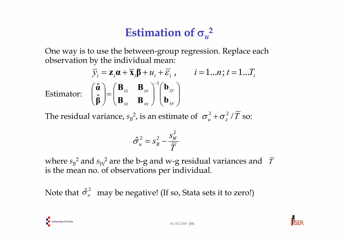
Estimation of σu2

One way is to use the between-group regression. Replace each observation by the individual mean:

Estimator:

The residual variance, sB2, is an estimate of so:

where sB2 and sW

2 are the b-g and w-g residual variances and is the mean no. of observations per individual.

Note that may be negative! (If so, Stata sets it to zero!)

iiiiii Ttniuy ...1;...1, ==+++= εβxαz

Tu /22εσσ +

Tss W

Bu

222ˆ −=σ

T

2ˆuσ

⎟⎟⎠

⎞⎜⎜⎝

⎛⎟⎟⎠

⎞⎜⎜⎝

⎛=⎟⎟

⎠

⎞⎜⎜⎝

⎛−

xy

zy

xxxz

zxzz

bb

BBBB

βα 1

ˆˆ

01/02/2007 (36)

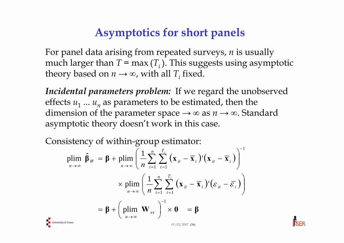
Asymptotics for short panelsFor panel data arising from repeated surveys, n is usually much larger than T = max (Ti ). This suggests using asymptotic theory based on n → ∞, with all Ti fixed.

Incidental parameters problem: If we regard the unobserved effects u1 ... un as parameters to be estimated, then the dimension of the parameter space → ∞ as n → ∞. Standard asymptotic theory doesn’t work in this case.

Consistency of within-group estimator:

( ) ( )

( ) ( )

β0Wβ

xx

xxxxββ

=×⎟⎠⎞

⎜⎝⎛+=

⎟⎟⎠

⎞⎜⎜⎝

⎛−−×

⎟⎟⎠

⎞⎜⎜⎝

⎛−−+=

−

∞→

= =∞→

−

= =∞→∞→

∑ ∑

∑ ∑

1

1 1

1

1 1

plim

'1plim

'1plimˆplim

xxn

n

i

T

tiitiit

n

n

i

T

tiitiit

nW

n

i

i

n

n

εε

01/02/2007 (1)

Day 3: Linear regression analysis: random effects

• Random effects regression: Testing the FE and RE assumptions

The Hausman test The Mundlak approach

• Endogeneity issuesForms of endogeneityEndogenous regressors: the between and within-group IV estimatorCorrelated individual effects: Hausman-Taylor estimation

01/02/2007 (2)

‘Random effects’ GLS & ML estimation•In general, since individuals are sampled at random from the population, ui (and all other variables) are random: so “random effects” is tautological•Extract the overall mean from ui :

yit = α0 + ziα + xit β + ui + εit

•Use Xi as shorthand for the person i’s time series xi1 … xiT •We may choose to assume that ui is uncorrelated with zi and Xi :

E(ui | zi , Xi ) = 0 ⇒ cov(ui , zi ) = 0 & cov(ui , Xi ) = 0•Assume also homoskedasticity and uncorrelatedness

E(ui2 | zi , Xi ) = σu

2 ; E(ui εit | zi , Xi ) = 0 for all t•Then write the composite random disturbance as:

vit = ui + εit

•What is the covariance structure of the random process vit ?

01/02/2007 (3)

Random effects covariance structure

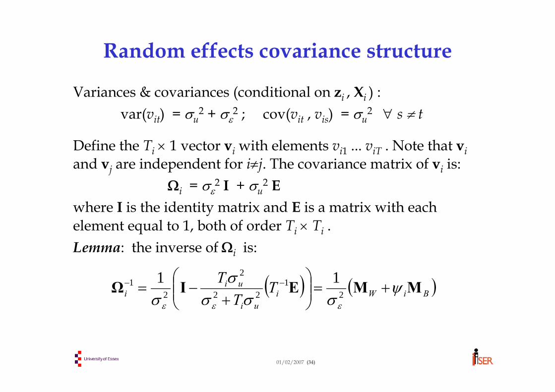
Variances & covariances (conditional on zi , Xi ) :var(vit) = σu

2 + σε2 ; cov(vit , vis) = σu2 for all s ≠ t

So the observations from different time periods (and the same individual) are not independent: they are equi-correlated.

The observations are clustered by individual, with non-zero intra-group correlations

The positive correlation between observations for any individual means that within-person variation is less than it would otherwise be. Consequently, whatever within-person variation we do have is particularly informative⇒ give more weight to within- than between-group variation

01/02/2007 (4)

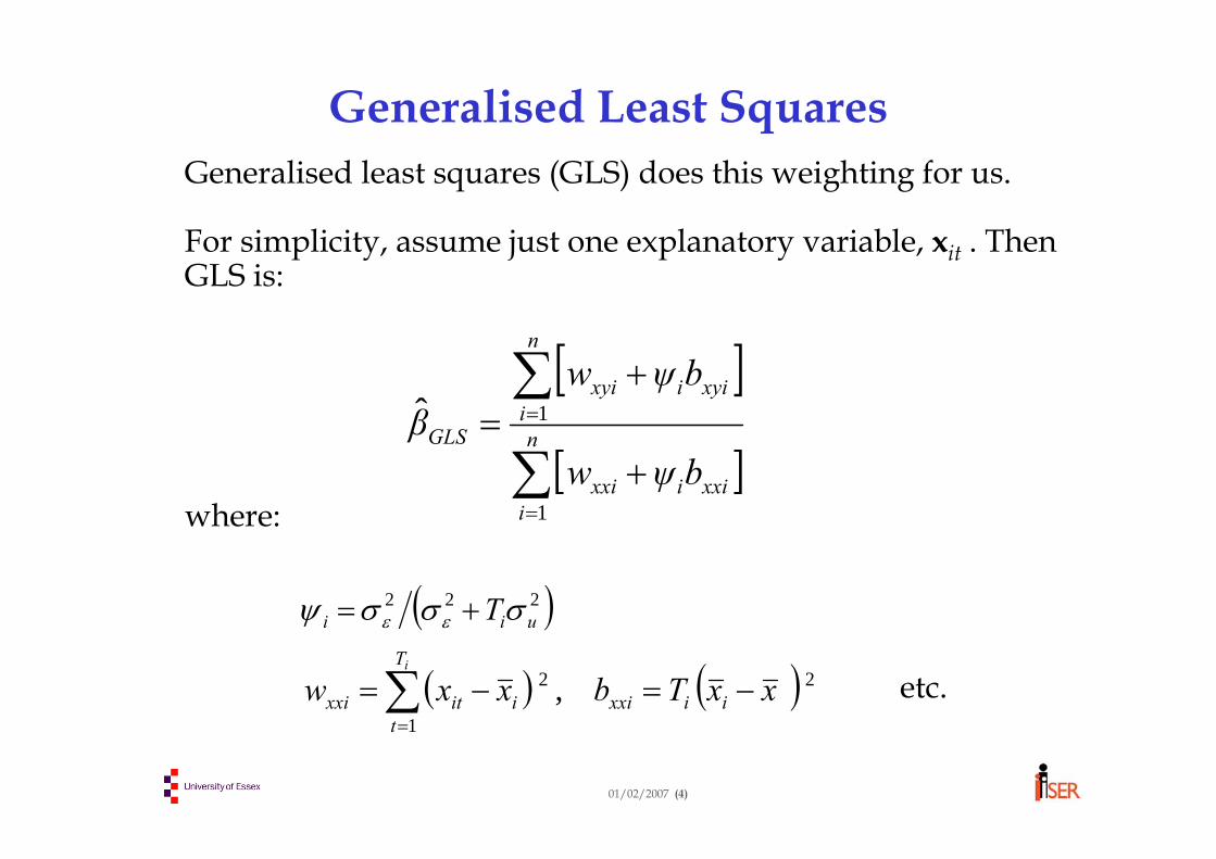
Generalised Least Squares Generalised least squares (GLS) does this weighting for us.

For simplicity, assume just one explanatory variable, xit . Then GLS is:

where:

etc.

[ ]

[ ]∑

∑

=

=

+

+= n

ixxiixxi

n

ixyiixyi

GLS

bψw

bψwβ

1

1ˆ

( ) ( ) 2

1

2 , xxTbxxw iixxi

T

tiitxxi

i

−=−=∑=

( )222 uii Tσσσψ εε +=

01/02/2007 (5)

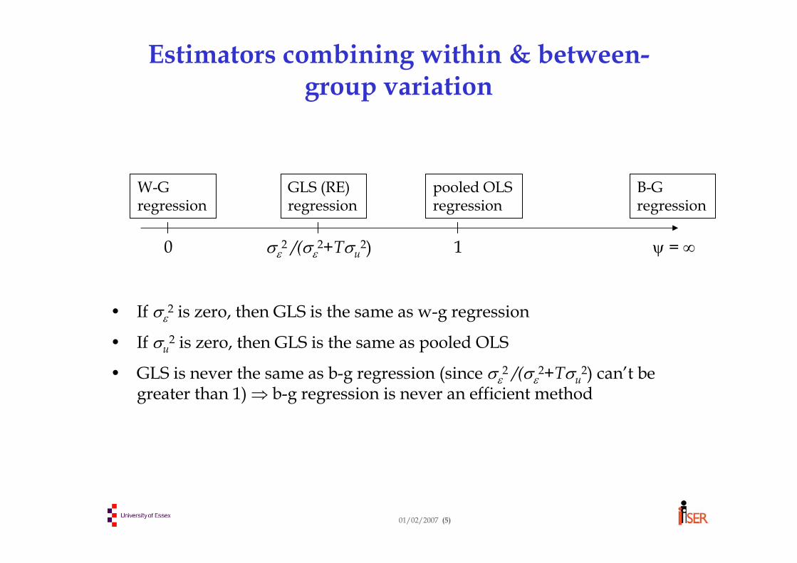
Estimators combining within & between-group variation

0 1 ψ = ∞

B-G regression

pooled OLS regression

W-G regression

GLS (RE) regression

σε2 /(σε

2+Tσu2)

• If σε2 is zero, then GLS is the same as w-g regression

• If σu2 is zero, then GLS is the same as pooled OLS

• GLS is never the same as b-g regression (since σε2 /(σε

2+Tσu2) can’t be

greater than 1) ⇒ b-g regression is never an efficient method

01/02/2007 (6)

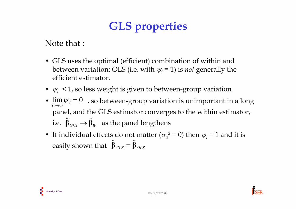
GLS propertiesNote that :

• GLS uses the optimal (efficient) combination of within and between variation: OLS (i.e. with ψi = 1) is not generally the efficient estimator.

• ψi < 1, so less weight is given to between-group variation• , so between-group variation is unimportant in a long

panel, and the GLS estimator converges to the within estimator, i.e. as the panel lengthens

• If individual effects do not matter (σu2 = 0) then ψi = 1 and it is

easily shown that

0lim =∞→ iTiψ

WGLS ββ ˆˆ →

OLSGLS ββ ˆˆ =

01/02/2007 (7)

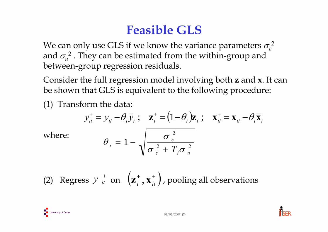
Feasible GLS We can only use GLS if we know the variance parameters σε2and σu

2 . They can be estimated from the within-group and between-group regression residuals. Consider the full regression model involving both z and x. It can be shown that GLS is equivalent to the following procedure:(1) Transform the data:

where:

(2) Regress on , pooling all observations

( ) iiititiiiiiitit yyy xxxzz θθθ −=−=−= +++ ;1;

+ity ( )++

iti xz ,

22

2

1ui

i T σσσθ

ε

ε

+−=

01/02/2007 (8)

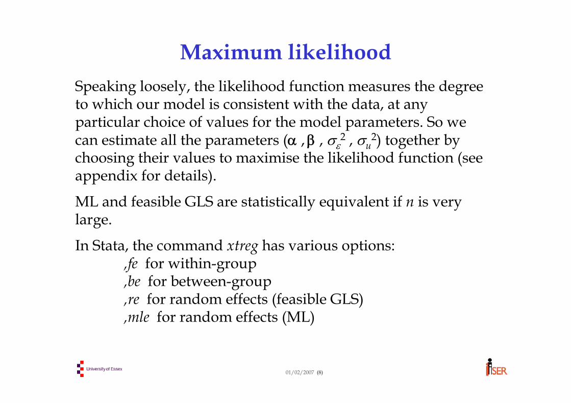
Maximum likelihood Speaking loosely, the likelihood function measures the degree to which our model is consistent with the data, at any particular choice of values for the model parameters. So we can estimate all the parameters (α , β , σε2 , σu

2) together by choosing their values to maximise the likelihood function (see appendix for details).

ML and feasible GLS are statistically equivalent if n is very large.

In Stata, the command xtreg has various options: ,fe for within-group,be for between-group,re for random effects (feasible GLS),mle for random effects (ML)

01/02/2007 (9)

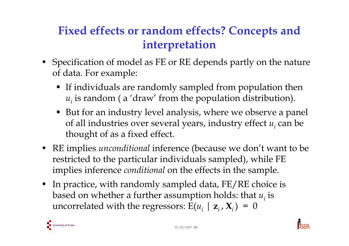
Fixed effects or random effects? Concepts and interpretation

• Specification of model as FE or RE depends partly on the natureof data. For example:

If individuals are randomly sampled from population then ui is random ( a ‘draw’ from the population distribution). But for an industry level analysis, where we observe a panel of all industries over several years, industry effect ui can be thought of as a fixed effect.

• RE implies unconditional inference (because we don’t want to be restricted to the particular individuals sampled), while FE implies inference conditional on the effects in the sample.

• In practice, with randomly sampled data, FE/RE choice is based on whether a further assumption holds: that ui is uncorrelated with the regressors: E(ui | zi , Xi ) = 0

01/02/2007 (10)

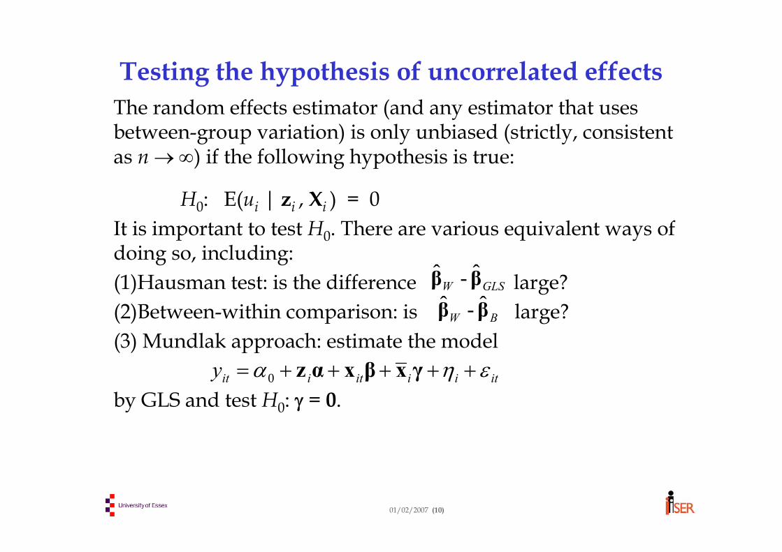
Testing the hypothesis of uncorrelated effectsThe random effects estimator (and any estimator that uses between-group variation) is only unbiased (strictly, consistentas n →∞) if the following hypothesis is true:

H0: E(ui | zi , Xi ) = 0It is important to test H0. There are various equivalent ways of doing so, including:(1)Hausman test: is the difference large?(2)Between-within comparison: is large?(3) Mundlak approach: estimate the model

by GLS and test H0: γ = 0. itiiitiity εηα +++++= γxβxαz0

GLSW ββ ˆ - ˆ

BW ββ ˆ - ˆ

01/02/2007 (11)

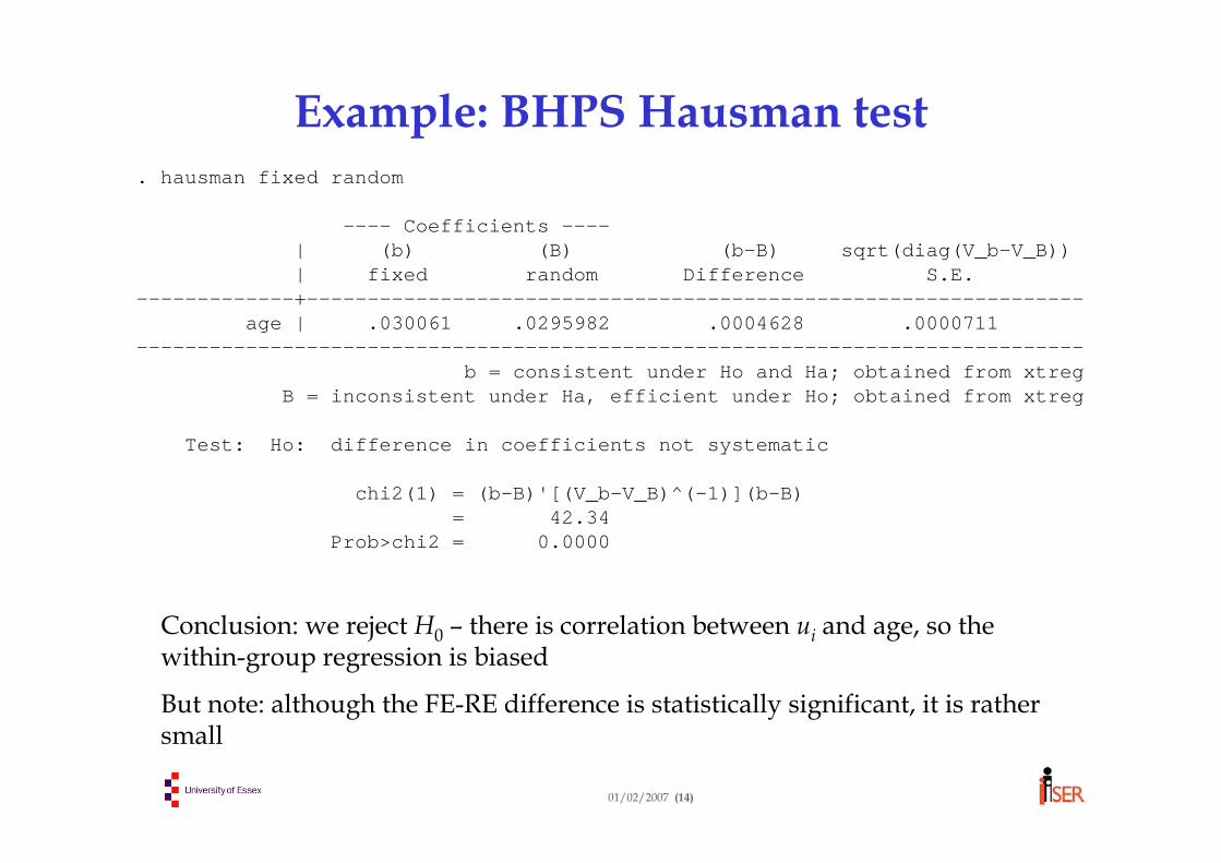
Hausman test The idea of the Hausman test is to compare two estimators which should be approximately the “same” if the zero-correlationassumption holds (H0), but different if the assumption is false (H1).Specifically, under H0 both estimators are unbiased (strictly, consistent), and is more efficient, (so ).It can be shown that the variance (matrix) of is:

Under H1 , is still unbiased but is not. So the Hausman test statistic:

should take a large value and reject if H0 is not true. If H0 is true, the statistic S is approximately distributed as χ2 with kd.f. where k = number of variables in xit , so we use critical values for the χ2(k) distribution.

GLSW ββ ˆ and ˆ

Wβ

GLSβ

GLSβ

)ˆ var( )ˆvar( GLSW ββ >

GLSW ββ ˆ - ˆ

( ) ( ) ( )GLSWGLSW ββββ ˆvarˆvarˆˆvar −=−

( ) ( ) ( )[ ] ( )GLSWGLSWGLSWS ββββββ ˆˆˆvarˆvar'ˆˆ 1−−−=

−

01/02/2007 (12)

BHPS example: feasible GLS estimates. xtreg lwage age cohort , re

Random-effects GLS regression Number of obs = 61516Group variable (i): pid Number of groups = 10335


Random effects u_i ~ Gaussian Wald chi2(2) = 7405.63corr(u_i, X) = 0 (assumed) Prob > chi2 = 0.0000

------------------------------------------------------------------------------lwage | Coef. Std. Err. z P>|z| [95% Conf. Interval]

-------------+----------------------------------------------------------------age | .0295982 .0003497 84.63 0.000 .0289127 .0302836

cohort | .0201181 .0004723 42.60 0.000 .0191924 .0210438_cons | -38.56221 .9343531 -41.27 0.000 -40.39351 -36.73091

-------------+----------------------------------------------------------------sigma_u | .49751772sigma_e | .28495079

rho | .75299116 (fraction of variance due to u_i)------------------------------------------------------------------------------

01/02/2007 (13)

BHPS example: within-group estimates. xtreg lwage age cohort , fe



F(1,51180) = 7094.59corr(u_i, Xb) = -0.4880 Prob > F = 0.0000


-------------+----------------------------------------------------------------age | .030061 .0003569 84.23 0.000 .0293615 .0307605

cohort | (dropped)_cons | .8994719 .01369 65.70 0.000 .8726394 .9263045

-------------+----------------------------------------------------------------sigma_u | .60455798sigma_e | .28494801


01/02/2007 (14)

Example: BHPS Hausman test. hausman fixed random

---- Coefficients ----| (b) (B) (b-B) sqrt(diag(V_b-V_B))| fixed random Difference S.E.

-------------+----------------------------------------------------------------age | .030061 .0295982 .0004628 .0000711

------------------------------------------------------------------------------b = consistent under Ho and Ha; obtained from xtreg

B = inconsistent under Ha, efficient under Ho; obtained from xtreg

Test: Ho: difference in coefficients not systematic

chi2(1) = (b-B)'[(V_b-V_B)^(-1)](b-B)= 42.34

Prob>chi2 = 0.0000

Conclusion: we reject H0 – there is correlation between ui and age, so the within-group regression is biased

But note: although the FE-RE difference is statistically significant, it is rather small

01/02/2007 (15)

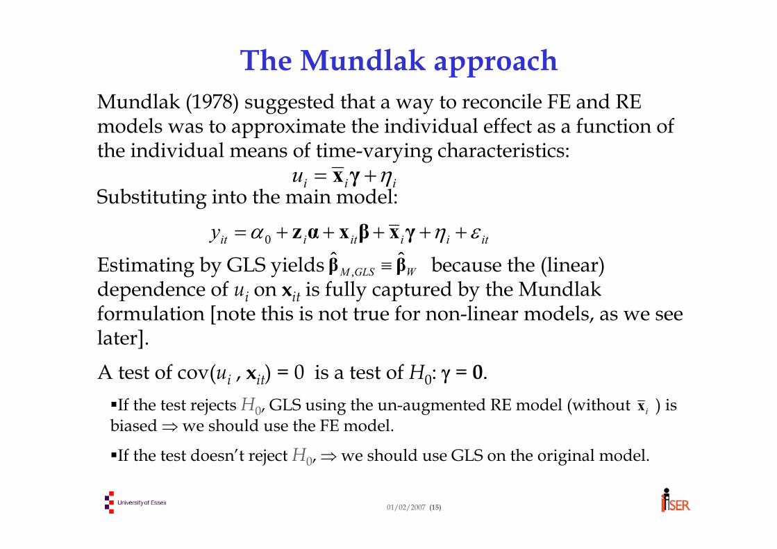
The Mundlak approachMundlak (1978) suggested that a way to reconcile FE and RE models was to approximate the individual effect as a function ofthe individual means of time-varying characteristics:

Substituting into the main model:

Estimating by GLS yields because the (linear) dependence of ui on xit is fully captured by the Mundlakformulation [note this is not true for non-linear models, as we seelater].

A test of cov(ui , xit) = 0 is a test of H0: γ = 0.If the test rejects H0, GLS using the un-augmented RE model (without ) is

biased ⇒ we should use the FE model.

If the test doesn’t reject H0, ⇒ we should use GLS on the original model.

itiiitiity εηα +++++= γxβxαz0

iiiu η+= γx

WGLSM ββ ˆˆ, ≡

ix

01/02/2007 (16)

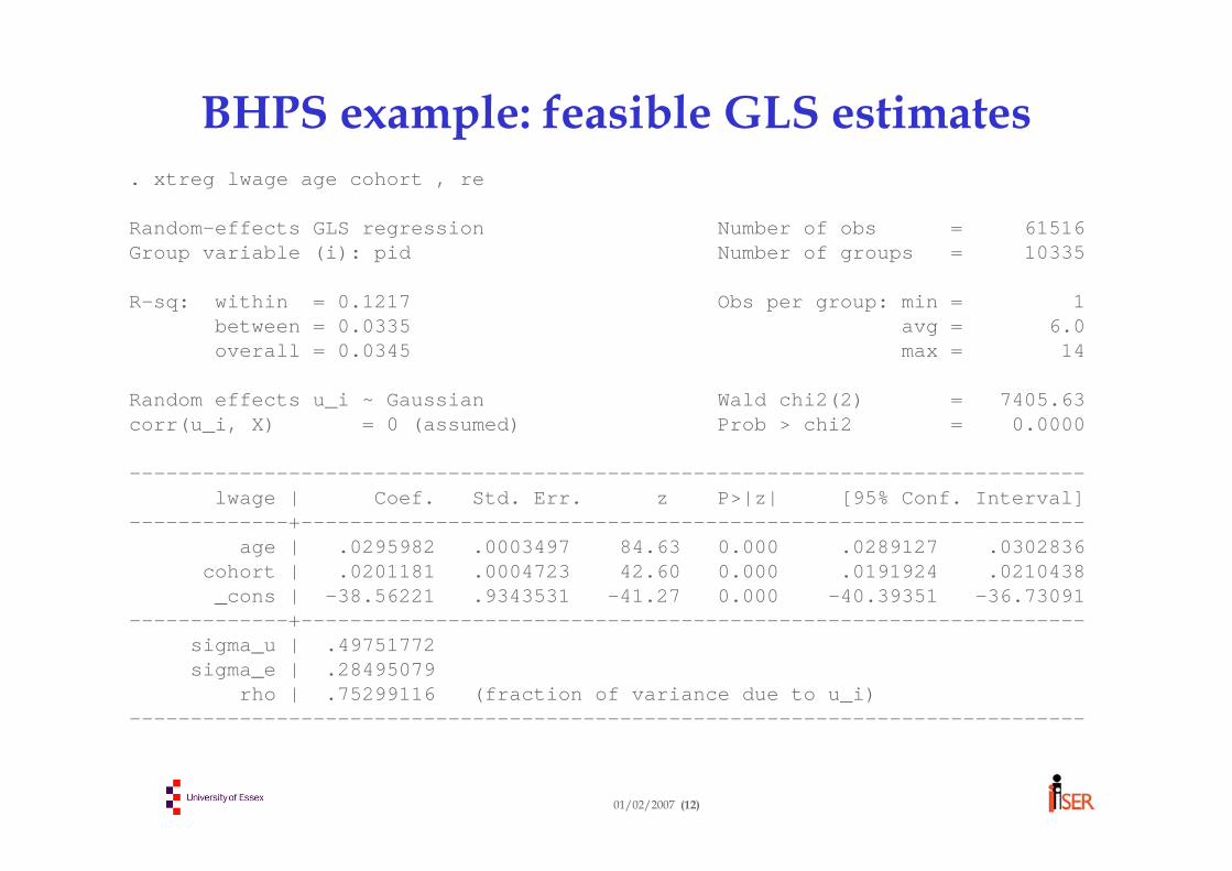
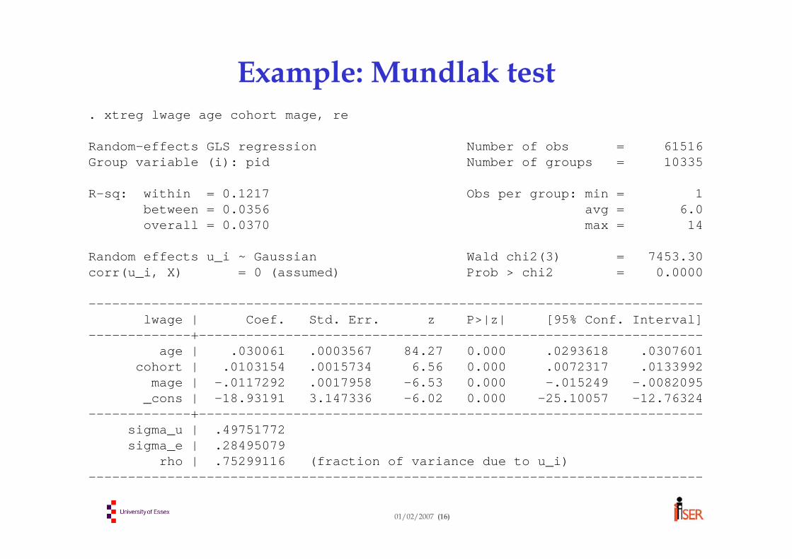
Example: Mundlak test. xtreg lwage age cohort mage, re

Random-effects GLS regression Number of obs = 61516Group variable (i): pid Number of groups = 10335


Random effects u_i ~ Gaussian Wald chi2(3) = 7453.30corr(u_i, X) = 0 (assumed) Prob > chi2 = 0.0000

------------------------------------------------------------------------------lwage | Coef. Std. Err. z P>|z| [95% Conf. Interval]

-------------+----------------------------------------------------------------age | .030061 .0003567 84.27 0.000 .0293618 .0307601

cohort | .0103154 .0015734 6.56 0.000 .0072317 .0133992mage | -.0117292 .0017958 -6.53 0.000 -.015249 -.0082095

_cons | -18.93191 3.147336 -6.02 0.000 -25.10057 -12.76324-------------+----------------------------------------------------------------

sigma_u | .49751772sigma_e | .28495079


01/02/2007 (17)

Endogeneity

• Forms of endogeneity• Endogenous regressors: the between and within-

group IV estimator• Correlated individual effects: Hausman-Taylor

estimation

01/02/2007 (18)

Endogeneity in static modelsExample: an earnings model

yit = α1 Educi + α2 Female + β1 Ageit + β2 Tenureit + ui + εit

Two forms of endogeneity:Two-way causation: experience is rewarded with high pay & workers tend

to stay in high-paid jobsUnobserved common factors: ability is rewarded with high pay & high-ability

people stay longer in education

Earnings Education

Unobserved ability

(a) unobserved common (b) 2-way causationfactor

Earnings

Tenure

01/02/2007 (19)

Example of endogeneityExample: an earnings model

yit = α1 Educi + α2 Female + β1 Ageit + β2 Tenureit + ui + εit

(1) Two-way causation: workers tend to stay in high-paid jobs:Tenure model: Tenureit = γ yit + υit (γ > 0)

= γ (α1 Educi + . . .+ β1 Ageit + β2 Tenureit + ui + εit) + υit

= [ γ (α1 Educi + . . .+ β1 Ageit + ui + εit) + υit ] / (1 - γ β2)⇒ cov(Tenureit , ui ) = γ σu

2/ (1 - γ β2) cov(Tenureit , εit) = γ σε

2/ (1 - γ β2)

(2) Unobserved common factors: ui represents ability & high-ability people stay longer in education:Educi = δui + other vars (δ > 0)⇒ cov(Educi , ui ) = δ σu

2

cov(Educi , εit) = 0

01/02/2007 (20)

Strategy for dealing with endogeneity

Within-group IV(w-g to eliminate ui and IV to deal with covariance with ε)

Cov(x,u) ≠ 0Cov(x,ε) ≠ 0

2-way causation (e.g. tenure → wage & wage → tenure)

GLS random effects regression

Cov(x,u) = 0Cov(x,ε) = 0

None

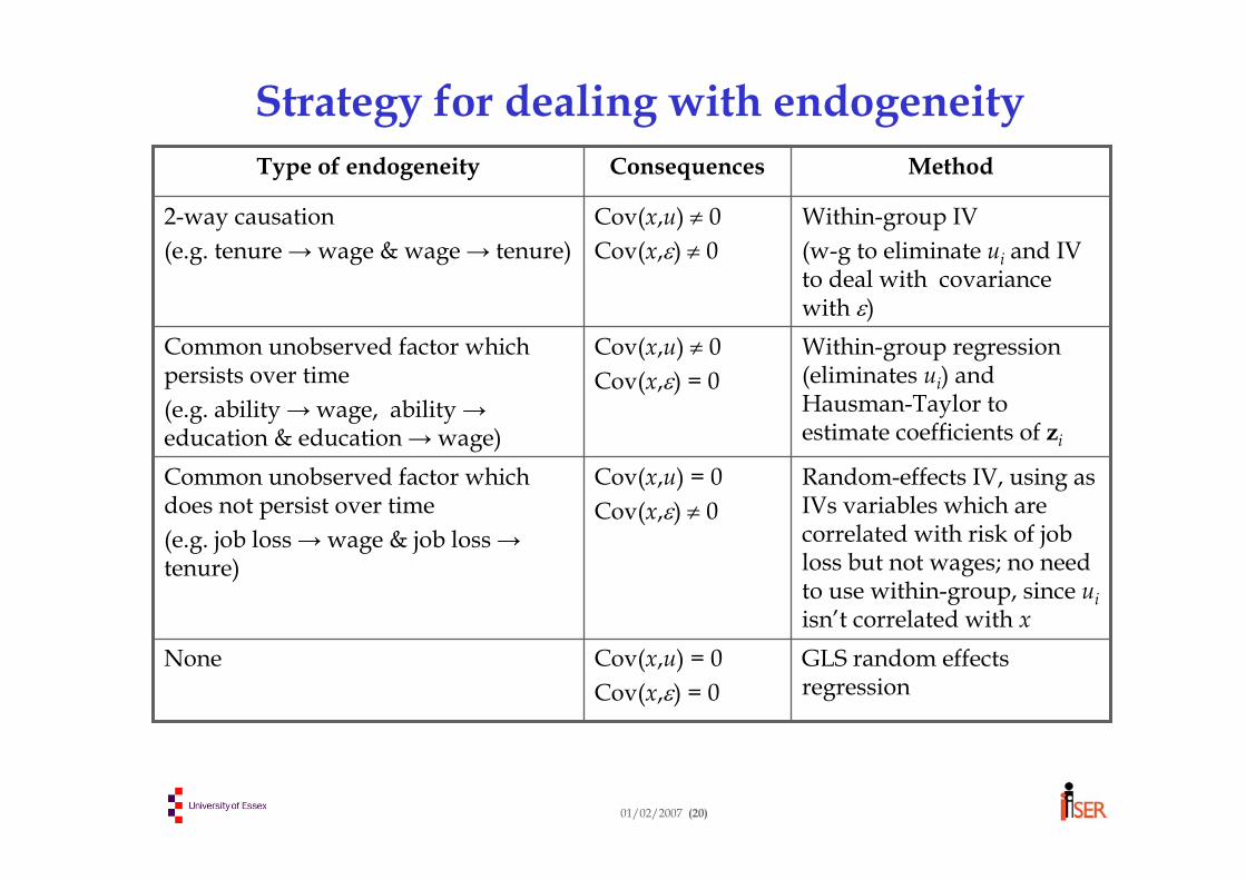
Random-effects IV, using as IVs variables which are correlated with risk of job loss but not wages; no need to use within-group, since uiisn’t correlated with x

Cov(x,u) = 0Cov(x,ε) ≠ 0

Common unobserved factor which does not persist over time (e.g. job loss → wage & job loss → tenure)

Within-group regression (eliminates ui) and Hausman-Taylor to estimate coefficients of zi

Cov(x,u) ≠ 0Cov(x,ε) = 0

Common unobserved factor which persists over time (e.g. ability → wage, ability → education & education → wage)

MethodConsequencesType of endogeneity

01/02/2007 (21)

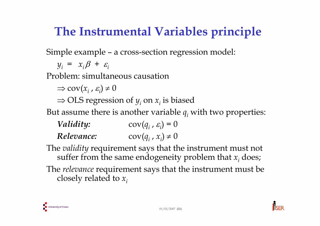
The Instrumental Variables principleSimple example – a cross-section regression model:

yi = xi β + εi

Problem: simultaneous causation ⇒ cov(xi , εi) ≠ 0⇒ OLS regression of yi on xi is biased

But assume there is another variable qi with two properties:Validity: cov(qi , εi) = 0 Relevance: cov(qi , xi) ≠ 0

The validity requirement says that the instrument must not suffer from the same endogeneity problem that xi does;

The relevance requirement says that the instrument must beclosely related to xi

01/02/2007 (22)

Motivation for the IV methodThe assumption of instrument validity is a moment condition

which states that a particular moment, cov(q, ε), must be equal to zero

But the model tells us that: εi = yi - xi β , so:cov(qi , εi) = cov(qi , [ yi -xi β ] )

= cov(qi , yi) - β cov(qi , xi ) = 0 (instrument validity requirement)

Solve for β:β = cov(qi , yi) / cov(qi , xi )

So, if q is a valid instrument, β must be equal to the ratio of the population covariance between q and y and between q and x.

01/02/2007 (23)

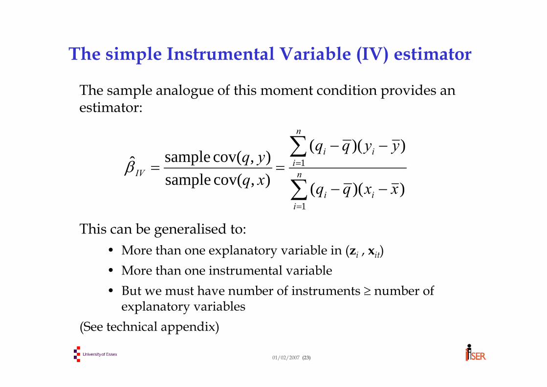
The simple Instrumental Variable (IV) estimator

The sample analogue of this moment condition provides an estimator:

This can be generalised to:• More than one explanatory variable in (zi , xit)• More than one instrumental variable• But we must have number of instruments ≥ number of

explanatory variables(See technical appendix)

∑

∑

=

=

−−

−−== n

iii

n

iii

IV

xxqq

yyqq

xqyq

1

1

))((

))((

),cov( sample),cov( sampleβ

01/02/2007 (24)

Simultaneity: Within-group IV estimationModel:


Partition xit :xit = (x1it , x2it),

Where x2it represents the endogenous covariates:cov(x1it , εit) = 0 and cov(x2it , εit) ≠ 0

Find a set of instruments q2it (at least as many as in x2it) where cov(q2it , εit) = 0

Full set of instruments: qit = (x1it , q2it)

Within-group transformation:

Within-group IV estimator uses as instruments iitiitiit yy εε −+−=− βxx )(

)( iit qq −

01/02/2007 (25)

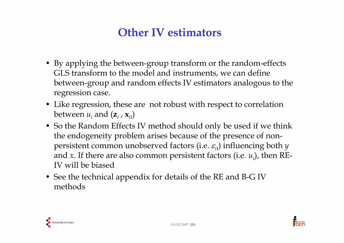
Other IV estimators

• By applying the between-group transform or the random-effects GLS transform to the model and instruments, we can define between-group and random effects IV estimators analogous to the regression case.

• Like regression, these are not robust with respect to correlation between ui and (zi , xit)

• So the Random Effects IV method should only be used if we think the endogeneity problem arises because of the presence of non-persistent common unobserved factors (i.e. εit) influencing both yand x. If there are also common persistent factors (i.e. ui), then RE-IV will be biased

• See the technical appendix for details of the RE and B-G IV methods

01/02/2007 (26)

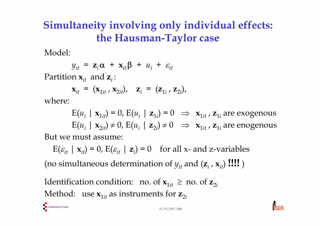
Simultaneity involving only individual effects:the Hausman-Taylor case

Model:yit = ziα + xit β + ui + εit

Partition xit and zi :xit = (x1it , x2it), zi = (z1i , z2i),

where: E(ui | x1it) = 0, E(ui | z1i) = 0 ⇒ x1it , z1i are exogenousE(ui | x2it) ≠ 0, E(ui | z2i) ≠ 0 ⇒ x1it , z1i are enogenous

But we must assume:E(εit | xit) = 0, E(εit | zi) = 0 for all x- and z-variables

(no simultaneous determination of yit and (zi , xit) !!!! )

Identification condition: no. of x1it ≥ no. of z2i

Method: use x1it as instruments for z2i

01/02/2007 (27)

The Hausman-Taylor (1981) estimatorStep 1: compute the within-group estimator for β:

⇒ regress on ⇒Step 2: construct within-group residuals & estimate σε

2 :

Step 3: estimate model for :

use as IVs qit = [x1it , z1i ] Step 4: Construct ; estimate σu

2 from Step 5: Carry out the random effects transform and estimate:

using as IVs

iit yy − iit xx − Wβ

( )( )xn

i

T

tit

Wiitiitit

kTn

yyi

−−=

−−−=

∑∑= =

1ˆˆ

ˆ)(ˆ

1 1

22 εσ

ε

ε

βxx

Wiii ye βx ˆˆ −= ... 1 , ... 1 residual, ˆ 0 iii Ttnie ==++= αzα

Wiiii ye βxαz ˆˆˆ* −−= *ˆ and ˆ iit eε

( ) ( ) ( ) ( )iiitiiiiitiiiiit uyy εθεθθθθ −+−+−+−=− 1)1( βxxαz

( )[ ]iiitiit 11 ,, xxxzq −=

01/02/2007 (28)

Endogeneity: BHPS examplesModel:

Ln wage = α0 + α1 Female + α2 Education beyond GCSE+ β1 Age + β2 Job tenure + u + ε

(1) Is job tenure jointly determined with the wage?• Use the standard IV/2SLS estimator in w-g form• Possible instruments: Married, Spouse part-time, Spouse full-time,

Dissatisfied with hours, • But are these valid instruments?

(2) Is educational attainment influenced by the same unobservable factors as labour market success?• Use the Hausman-Taylor estimator• Instruments come from within the model• But is everything uncorrelated with ε ?

01/02/2007 (29)

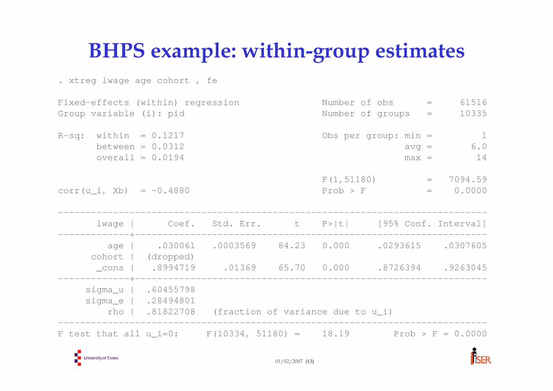
Within-group regression. xtreg logearn age postGCSE tenure, fe



F(3,30701) = 1115.13corr(u_i, Xb) = -0.4195 Prob > F = 0.0000

------------------------------------------------------------------------------logearn | Coef. Std. Err. t P>|t| [95% Conf. Interval]

-------------+----------------------------------------------------------------age | .0249189 .0004778 52.16 0.000 .0239824 .0258554

postGCSE | .0263467 .0089311 2.95 0.003 .0088413 .043852tenure | .0016804 .0004299 3.91 0.000 .0008377 .002523_cons | .9805382 .0174738 56.11 0.000 .9462889 1.014787

-------------+----------------------------------------------------------------sigma_u | .54846498sigma_e | .24922759


01/02/2007 (30)

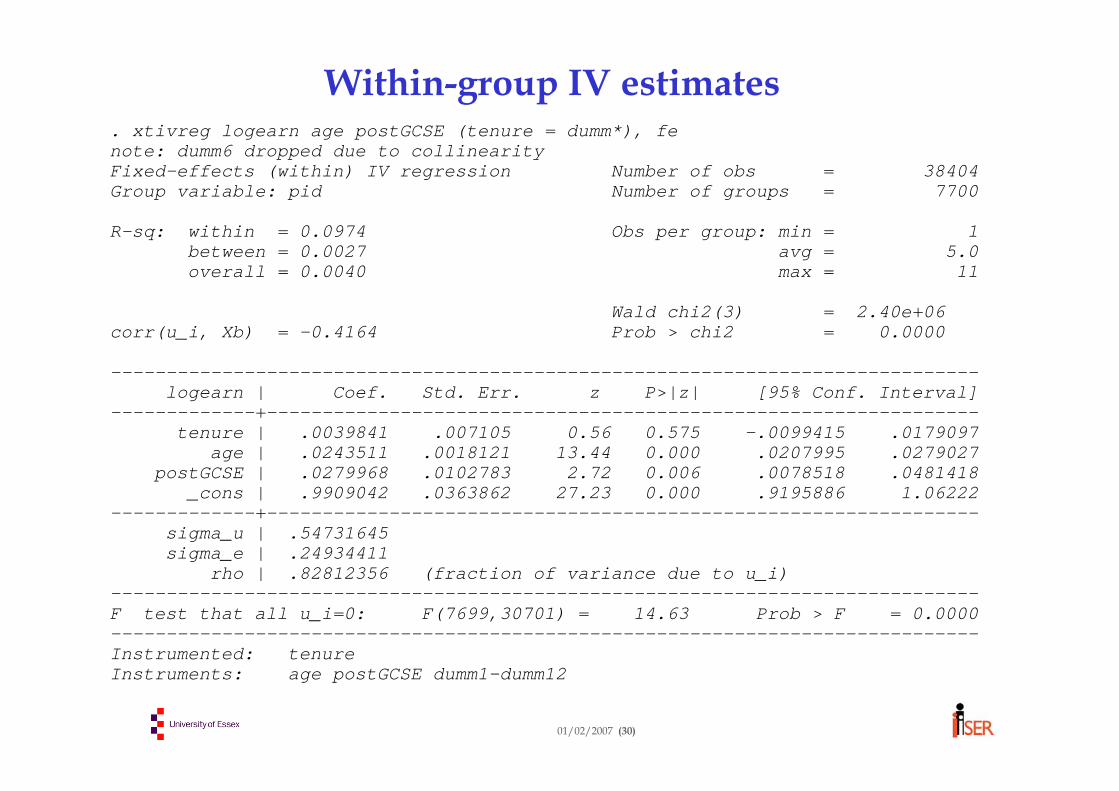
Within-group IV estimates. xtivreg logearn age postGCSE (tenure = dumm*), fenote: dumm6 dropped due to collinearityFixed-effects (within) IV regression Number of obs = 38404Group variable: pid Number of groups = 7700


Wald chi2(3) = 2.40e+06corr(u_i, Xb) = -0.4164 Prob > chi2 = 0.0000

------------------------------------------------------------------------------logearn | Coef. Std. Err. z P>|z| [95% Conf. Interval]

-------------+----------------------------------------------------------------tenure | .0039841 .007105 0.56 0.575 -.0099415 .0179097

age | .0243511 .0018121 13.44 0.000 .0207995 .0279027postGCSE | .0279968 .0102783 2.72 0.006 .0078518 .0481418

_cons | .9909042 .0363862 27.23 0.000 .9195886 1.06222-------------+----------------------------------------------------------------

sigma_u | .54731645sigma_e | .24934411

rho | .82812356 (fraction of variance due to u_i)------------------------------------------------------------------------------F test that all u_i=0: F(7699,30701) = 14.63 Prob > F = 0.0000------------------------------------------------------------------------------Instrumented: tenureInstruments: age postGCSE dumm1-dumm12

01/02/2007 (31)

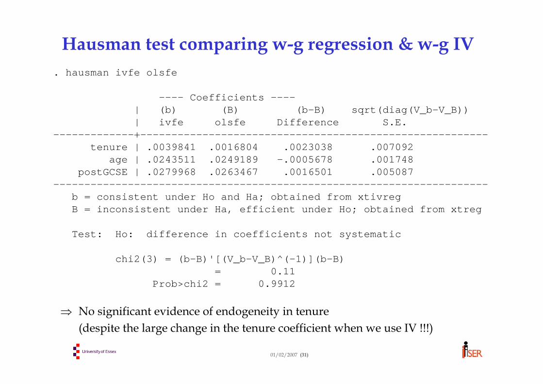
Hausman test comparing w-g regression & w-g IV. hausman ivfe olsfe

---- Coefficients ----| (b) (B) (b-B) sqrt(diag(V_b-V_B))| ivfe olsfe Difference S.E.

-------------+--------------------------------------------------------tenure | .0039841 .0016804 .0023038 .007092

age | .0243511 .0249189 -.0005678 .001748postGCSE | .0279968 .0263467 .0016501 .005087

----------------------------------------------------------------------b = consistent under Ho and Ha; obtained from xtivregB = inconsistent under Ha, efficient under Ho; obtained from xtreg

Test: Ho: difference in coefficients not systematic

chi2(3) = (b-B)'[(V_b-V_B)^(-1)](b-B)= 0.11

Prob>chi2 = 0.9912

⇒ No significant evidence of endogeneity in tenure (despite the large change in the tenure coefficient when we use IV !!!)

01/02/2007 (32)

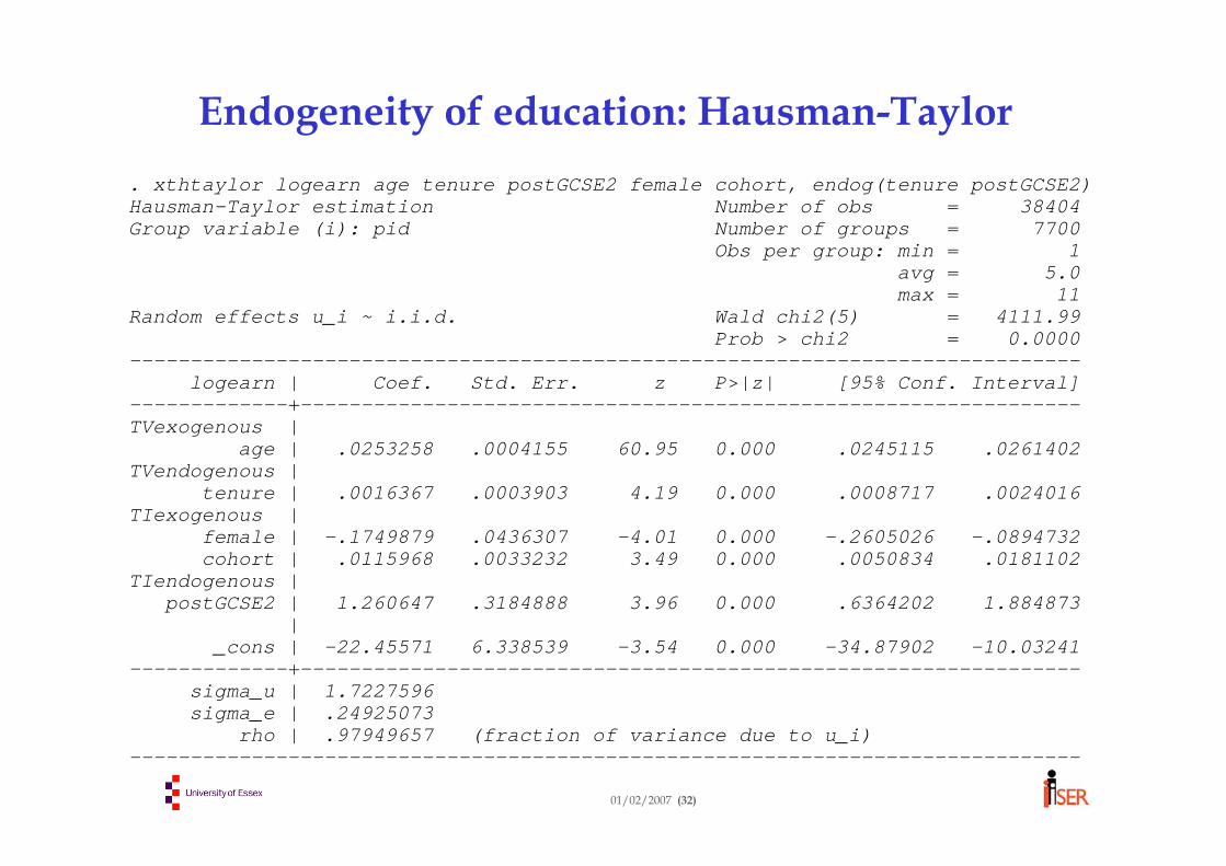
Endogeneity of education: Hausman-Taylor. xthtaylor logearn age tenure postGCSE2 female cohort, endog(tenure postGCSE2) Hausman-Taylor estimation Number of obs = 38404Group variable (i): pid Number of groups = 7700

Obs per group: min = 1avg = 5.0max = 11

Random effects u_i ~ i.i.d. Wald chi2(5) = 4111.99Prob > chi2 = 0.0000

------------------------------------------------------------------------------logearn | Coef. Std. Err. z P>|z| [95% Conf. Interval]

-------------+----------------------------------------------------------------TVexogenous |

age | .0253258 .0004155 60.95 0.000 .0245115 .0261402TVendogenous |

tenure | .0016367 .0003903 4.19 0.000 .0008717 .0024016TIexogenous |

female | -.1749879 .0436307 -4.01 0.000 -.2605026 -.0894732cohort | .0115968 .0033232 3.49 0.000 .0050834 .0181102

TIendogenous |postGCSE2 | 1.260647 .3184888 3.96 0.000 .6364202 1.884873

|_cons | -22.45571 6.338539 -3.54 0.000 -34.87902 -10.03241

-------------+----------------------------------------------------------------sigma_u | 1.7227596sigma_e | .24925073


01/02/2007 (33)

Technical appendix 1: random effects


01/02/2007 (34)

Random effects covariance structure

Variances & covariances (conditional on zi , Xi ) :var(vit) = σu

2 + σε2 ; cov(vit , vis) = σu2 ∀ s ≠ t

Define the Ti × 1 vector vi with elements vi1 ... viT . Note that viand vj are independent for i≠j. The covariance matrix of vi is:

Ωi = σε2 I + σu2 E

where I is the identity matrix and E is a matrix with each element equal to 1, both of order Ti × Ti .Lemma: the inverse of Ωi is:

( ) ( )BiWiui

uii T

TT MMEIΩ ψ

σσσσ

σ εεε

+=⎟⎟⎠

⎞⎜⎜⎝

⎛+

−= −−2

122

2

21 11

01/02/2007 (35)

Within- and between-group transformations

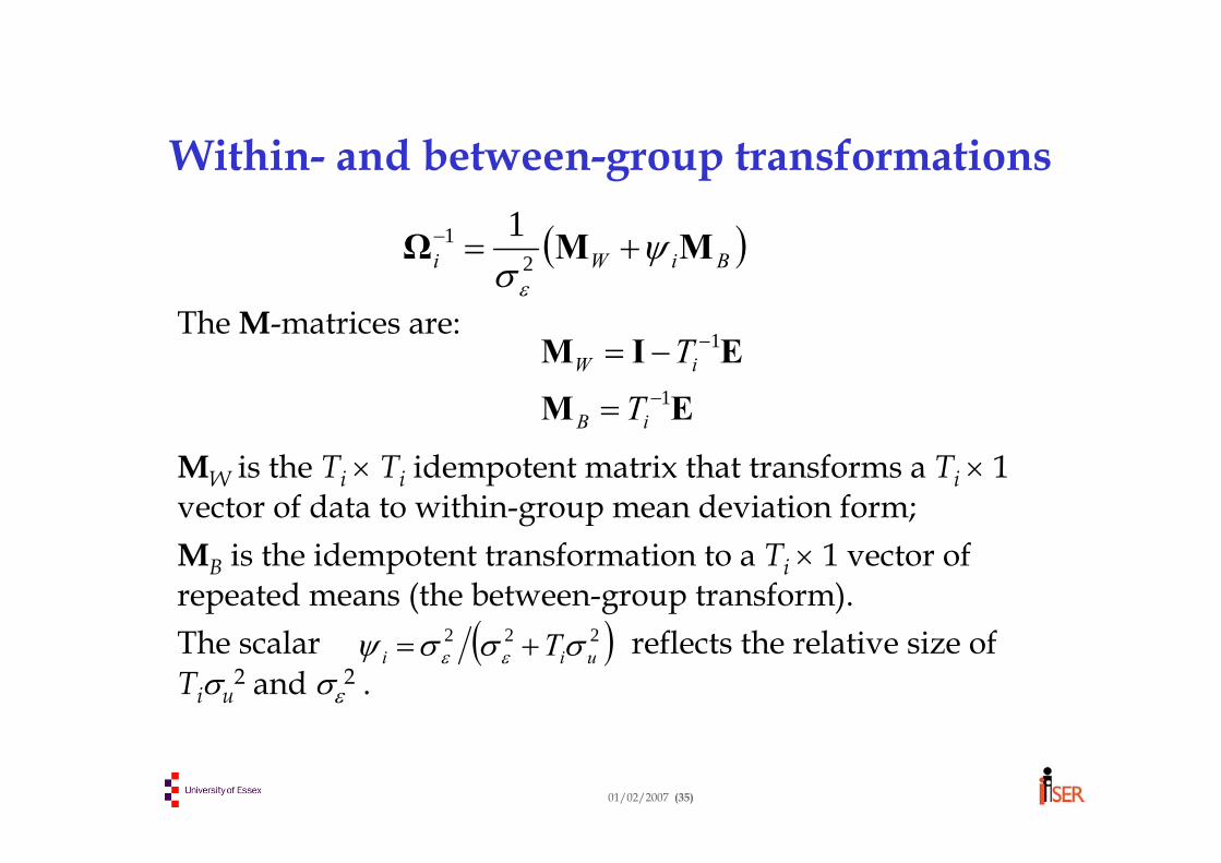
The M-matrices are:

MW is the Ti × Ti idempotent matrix that transforms a Ti × 1 vector of data to within-group mean deviation form; MB is the idempotent transformation to a Ti × 1 vector of repeated means (the between-group transform).The scalar reflects the relative size of Tiσu

2 and σε2 .

EM

EIM1

1

−

−

=

−=

iB

iW

T

T

( )222 uii Tσσσψ εε +=

( )BiWi MMΩ ψσε

+=−2

1 1

01/02/2007 (36)

Generalised Least SquaresFor simplicity, subsume zi within xit . Then GLS is:

where , etc.

[ ] [ ]∑∑

∑∑

=

−

=

=

−−

=

−

+⎟⎠

⎞⎜⎝

⎛+=

⎟⎠

⎞⎜⎝

⎛=

n

iixyiixyi

n

ixxiixxi

n

iiii

n

iiiiGLS

1

1

1

1

11

1

1 ''ˆ

bwBW

yΩXXΩXβ

ψψ

( ) ( ) iiixxi

T

tiitiitxxi T

i

xxBxxxxW ','1

=−−=∑=

01/02/2007 (37)

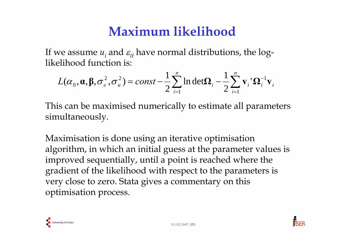
Maximum likelihood If we assume ui and εit have normal distributions, the log-likelihood function is:

This can be maximised numerically to estimate all parameters simultaneously.

Maximisation is done using an iterative optimisation algorithm, in which an initial guess at the parameter values is improved sequentially, until a point is reached where the gradient of the likelihood with respect to the parameters is very close to zero. Stata gives a commentary on this optimisation process.

∑∑=

−

=

−−=n

iiii

n

iiu constL

1

1

1

220 '

21detln

21),,,,( vΩvΩβα σσα ε

01/02/2007 (38)

Technical appendix 2: instrumental variables


01/02/2007 (39)

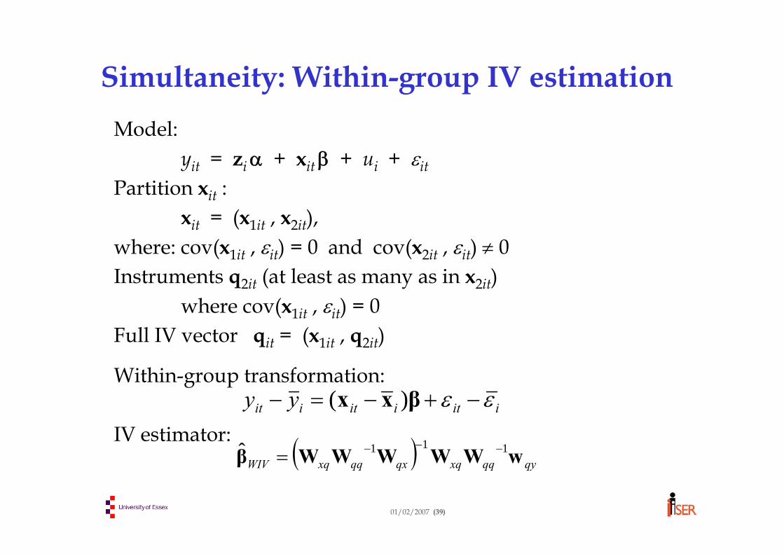
Simultaneity: Within-group IV estimationModel:


Partition xit :xit = (x1it , x2it),

where: cov(x1it , εit) = 0 and cov(x2it , εit) ≠ 0Instruments q2it (at least as many as in x2it)

where cov(x1it , εit) = 0Full IV vector qit = (x1it , q2it)

Within-group transformation:

IV estimator:iitiitiit yy εε −+−=− βxx )(

( ) qyqqxqqxqqxqWIV wWWWWWβ 111ˆ −−−=

01/02/2007 (40)

Consistency

β

wWW

WWWββ

=

⎟⎟⎠

⎞⎜⎜⎝

⎛⎟⎠⎞

⎜⎝⎛

×⎟⎟⎠

⎞⎜⎜⎝

⎛⎟⎠⎞

⎜⎝⎛+=

∞→

−

∞→∞→

−

∞→

−

∞→∞→∞→

εqn

qqn

xqn

qxn

qqn

xqn

WIVn

nnn

nnn

1plim1plim1plim

1plim1plim1plimˆplim

1

11

This consistency property holds because:• The within-group transform removes ui , which may be

correlated with x2it

• The instruments are uncorrelated with ε, so:

( ) ( ) 0qqw =−−= ∑∑= =∞→∞→

n

i

T

tiitiit

nq

n

i

nn 1 1'1plim1plim εεε

01/02/2007 (41)

Between-group IV estimator

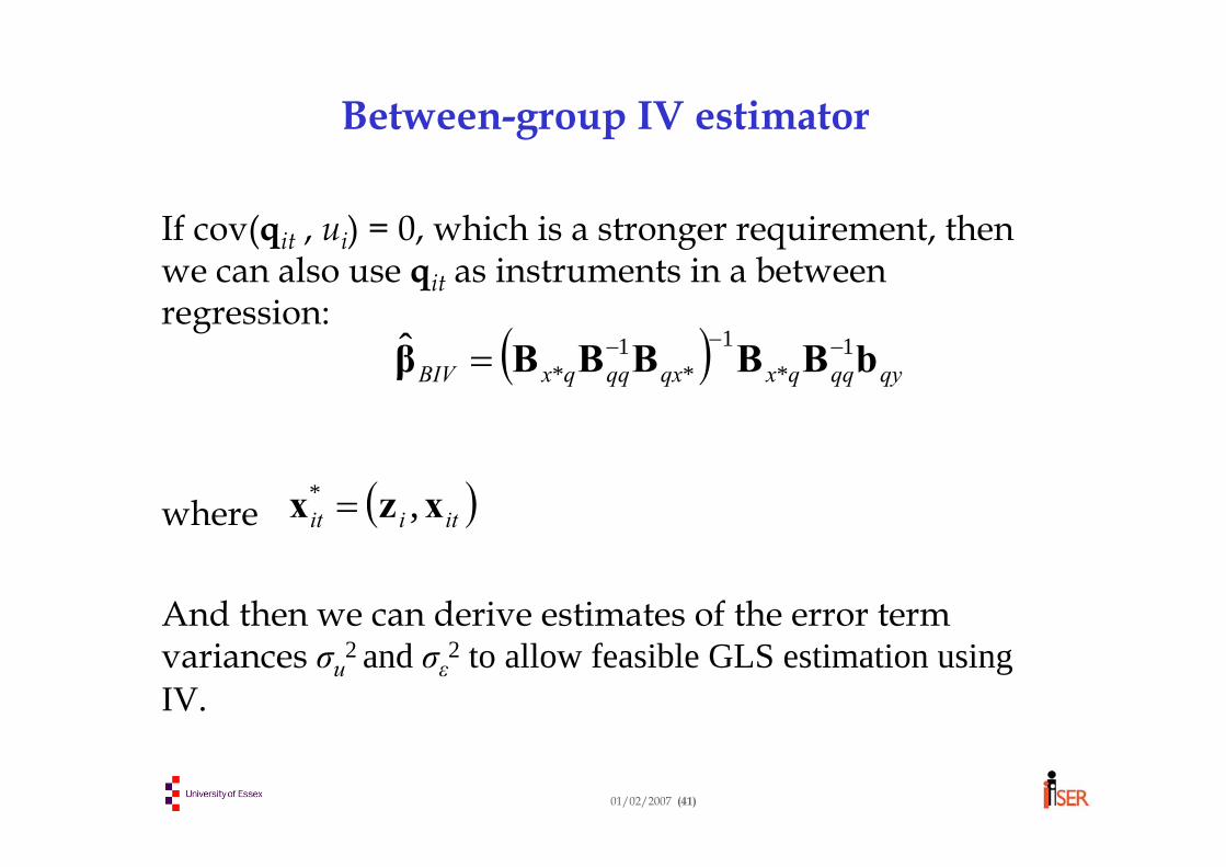
If cov(qit , ui) = 0, which is a stronger requirement, then we can also use qit as instruments in a between regression:

where

And then we can derive estimates of the error term variances σu2 and σε2 to allow feasible GLS estimation using IV.

( ) qyqqqxqxqqqxBIV bBBBBBβ 1*

1*

1*

ˆ −−−=

( )itiit xzx ,* =

01/02/2007 (42)

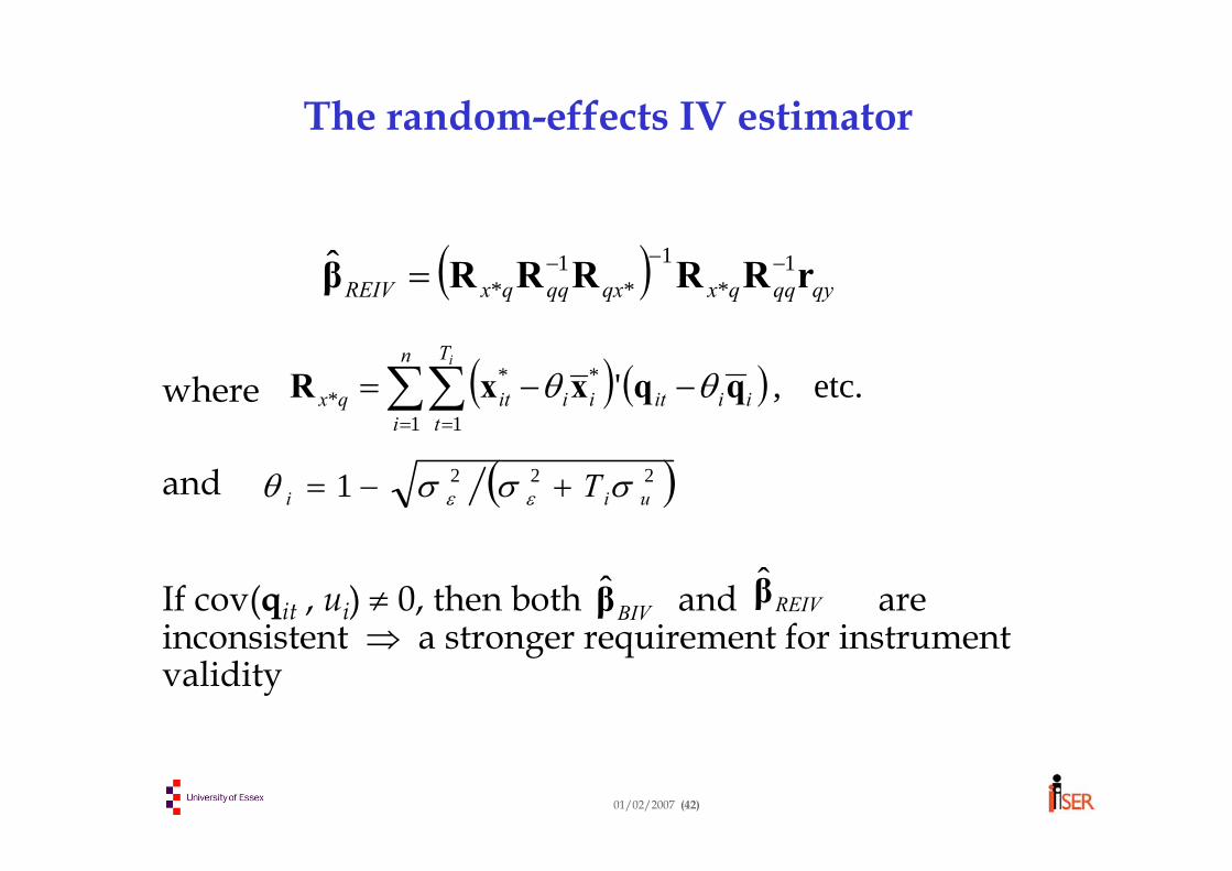
The random-effects IV estimator

where

and

If cov(qit , ui) ≠ 0, then both and are inconsistent ⇒ a stronger requirement for instrument validity

( ) qyqqqxqxqqqxREIV rRRRRRβ 1*

1*

1*

ˆ −−−=

( ) ( ) etc.,'1 1

*** ∑∑

= =

−−=n

i

T

tiiitiiitqx

i

qqxxR θθ

( )2221 uii T σσσθ εε +−=

BIVβ REIVβ

01/02/2007 (1)

Day 4: Binary response models

• Types of discrete variables • Linear regression • Latent linear regression• Conditional (fixed-effects) logit• Random effects logit and probit

01/02/2007 (2)

Forms of discretenessCensoring/corner solutions generate variables which are mixed discrete/continuous (e.g. hours of work are 0 for non-employed, any positive value for employees)

Truncation involves discarding part of the population (e.g. low-income targeted samples, or earnings models for employees only)

Count variables are the outcome of some counting process (e.g. the number of durables owned, or the number of employees of a firm)

Binary variables reflect a distinction between two states (e.g. unemployed or not, married or not)

Ordinal variables are ordered variables, possibly taking more than two values(e.g. happiness on a scale 1=miserable … 5=ecstatic; rank in the army)

Unordered variables reflect outcomes which are discrete but with no natural ordering(e.g. choice of occupation)

01/02/2007 (3)

Binary models (1)

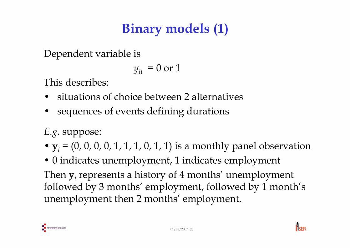
Dependent variable is yit = 0 or 1

This describes:• situations of choice between 2 alternatives• sequences of events defining durations

E.g. suppose:• yi = (0, 0, 0, 0, 1, 1, 1, 0, 1, 1) is a monthly panel observation• 0 indicates unemployment, 1 indicates employmentThen yi represents a history of 4 months’ unemployment followed by 3 months’ employment, followed by 1 month’s unemployment then 2 months’ employment.

01/02/2007 (4)

Binary models (2)

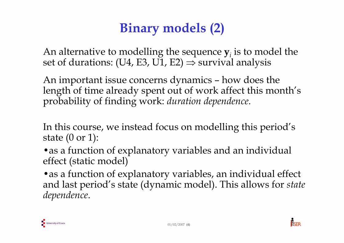
An alternative to modelling the sequence yi is to model the set of durations: (U4, E3, U1, E2) ⇒ survival analysis

An important issue concerns dynamics – how does the length of time already spent out of work affect this month’s probability of finding work: duration dependence.

In this course, we instead focus on modelling this period’s state (0 or 1):•as a function of explanatory variables and an individual effect (static model)•as a function of explanatory variables, an individual effect and last period’s state (dynamic model). This allows for state dependence.

01/02/2007 (5)

Why are special methods needed ?

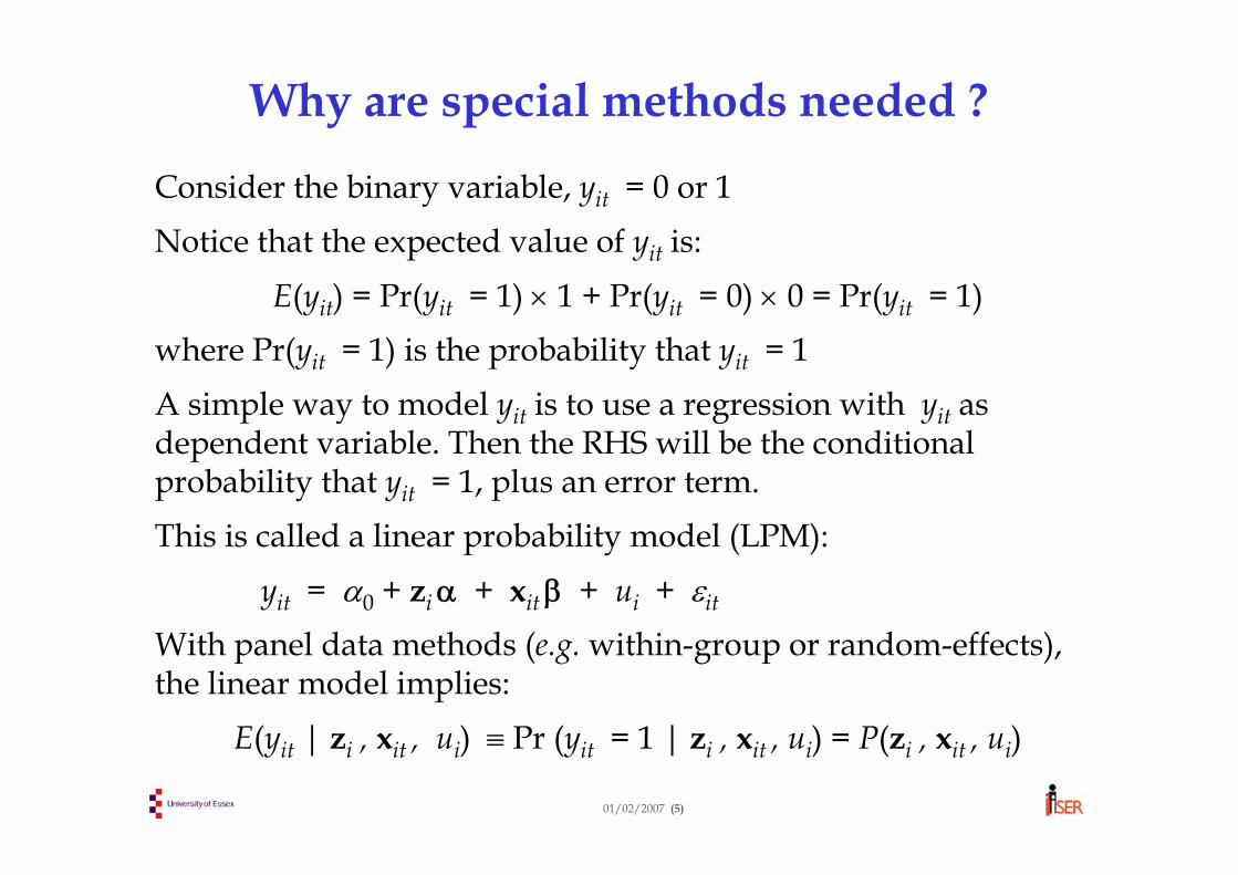
Consider the binary variable, yit = 0 or 1Notice that the expected value of yit is:

E(yit) = Pr(yit = 1) × 1 + Pr(yit = 0) × 0 = Pr(yit = 1)where Pr(yit = 1) is the probability that yit = 1A simple way to model yit is to use a regression with yit as dependent variable. Then the RHS will be the conditional probability that yit = 1, plus an error term.This is called a linear probability model (LPM):

yit = α0 + ziα + xit β + ui + εit

With panel data methods (e.g. within-group or random-effects), the linear model implies:

E(yit | zi , xit , ui) ≡ Pr (yit = 1 | zi , xit , ui) = P(zi , xit , ui)

01/02/2007 (6)

Disadvantages of the LPM

The linear probability model requires:

P(zi , xit , ui) ≈ α0 + ziα + xit β + ui

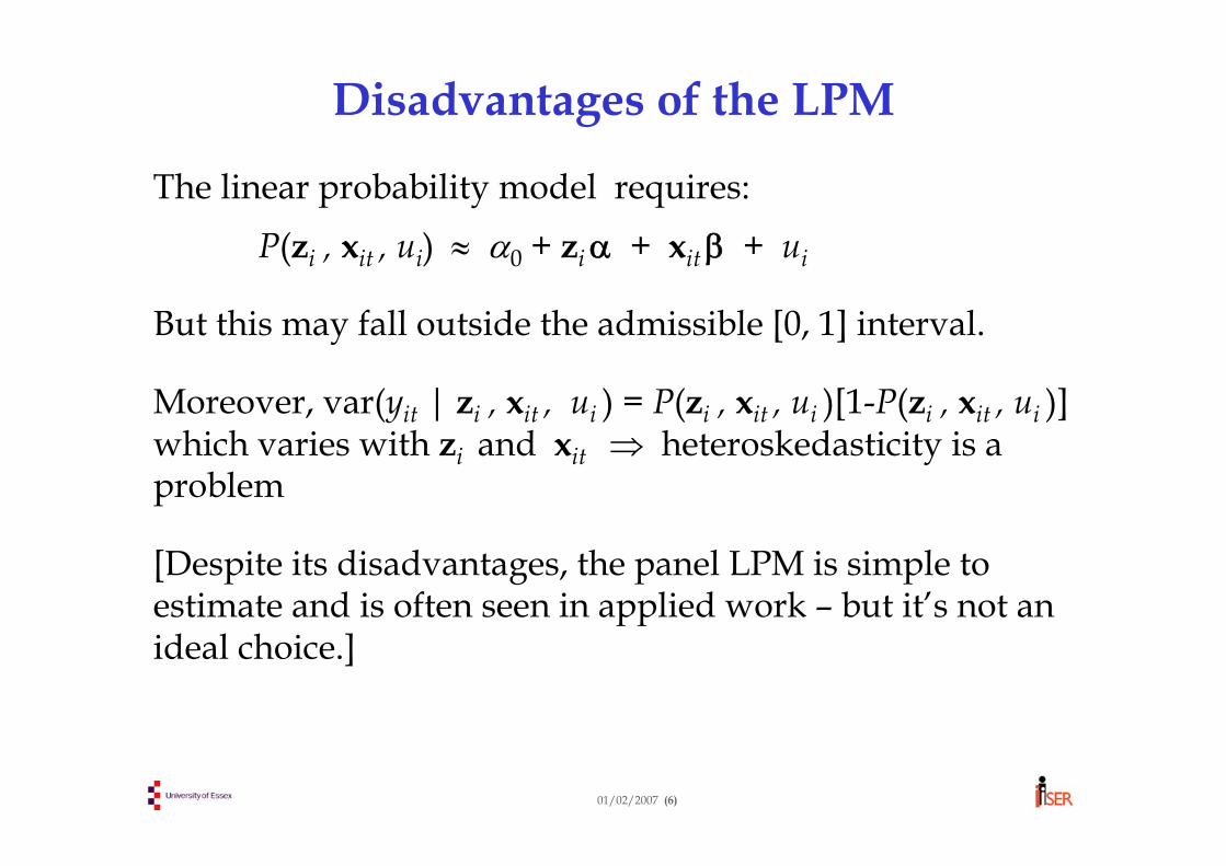
But this may fall outside the admissible [0, 1] interval.

Moreover, var(yit | zi , xit , ui ) = P(zi , xit , ui )[1-P(zi , xit , ui )]which varies with zi and xit ⇒ heteroskedasticity is a problem

[Despite its disadvantages, the panel LPM is simple to estimate and is often seen in applied work – but it’s not an ideal choice.]

01/02/2007 (7)

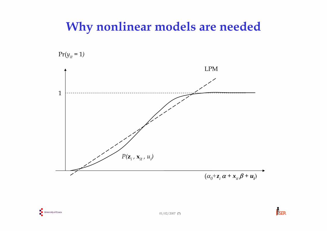
Why nonlinear models are needed

(α0+zi α + xit β + ui)

1

Pr(yit = 1)

LPM

P(zi , xit , ui)

01/02/2007 (8)

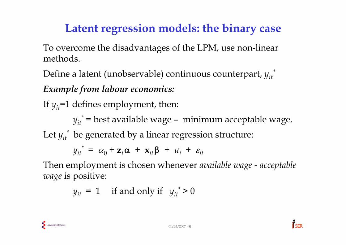
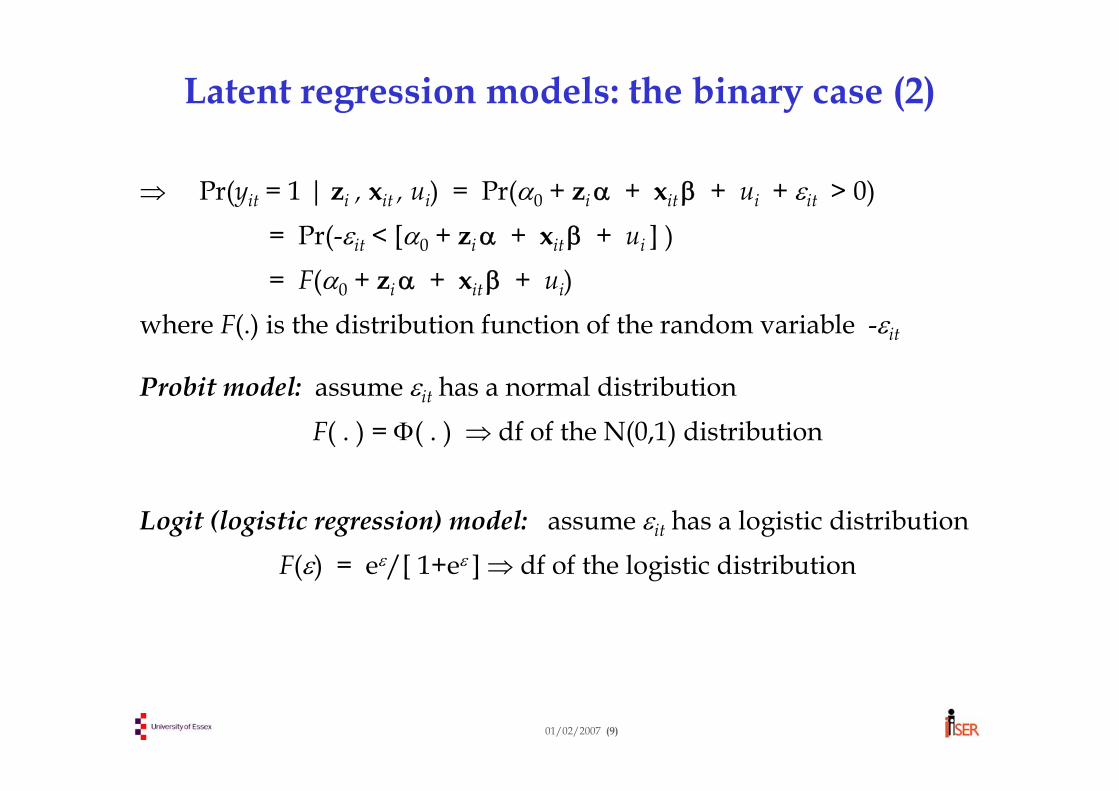
Latent regression models: the binary caseTo overcome the disadvantages of the LPM, use non-linear methods.Define a latent (unobservable) continuous counterpart, yit

*

Example from labour economics:If yit=1 defines employment, then:

yit* = best available wage – minimum acceptable wage.

Let yit* be generated by a linear regression structure:

yit* = α0 + ziα + xit β + ui + εit

Then employment is chosen whenever available wage - acceptablewage is positive:

yit = 1 if and only if yit* > 0

01/02/2007 (9)

Latent regression models: the binary case (2)

⇒ Pr(yit = 1 | zi , xit , ui) = Pr(α0 + zi α + xit β + ui + εit > 0)= Pr(-εit < [α0 + zi α + xit β + ui ] )= F(α0 + zi α + xit β + ui)

where F(.) is the distribution function of the random variable -εit

Probit model: assume εit has a normal distributionF( . ) = Φ( . ) ⇒ df of the N(0,1) distribution

Logit (logistic regression) model: assume εit has a logistic distributionF(ε) = eε/[ 1+eε ] ⇒ df of the logistic distribution

01/02/2007 (10)

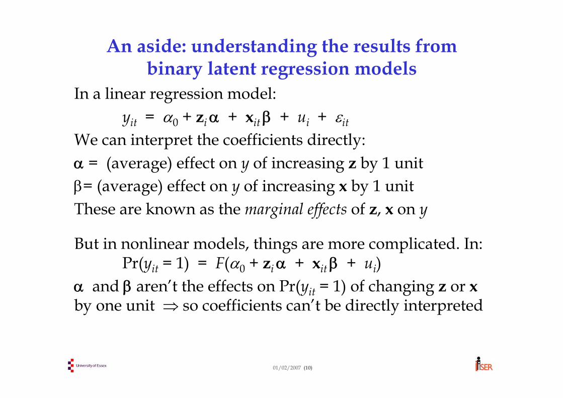
An aside: understanding the results from binary latent regression models

In a linear regression model:yit = α0 + zi α + xit β + ui + εit

We can interpret the coefficients directly:α = (average) effect on y of increasing z by 1 unitβ= (average) effect on y of increasing x by 1 unitThese are known as the marginal effects of z, x on y

But in nonlinear models, things are more complicated. In:Pr(yit = 1) = F(α0 + zi α + xit β + ui)

α and β aren’t the effects on Pr(yit = 1) of changing z or xby one unit ⇒ so coefficients can’t be directly interpreted

01/02/2007 (11)

Some concepts for summarising resultsModel: Pr(yit = 1) = F(α0 + zi α + xit β + ui) (call this conditional probability Pit)

Coefficients = α0 , zi and βPredicted probability = Pit

Odds (Oit) = Pit / (1 – Pit )For 2 people with different z and x –values, whose probabilities of y=1 are P0 and P1 :Odds ratio = O1 /O0

Relative risk = P1 /P0

Relative risk and the odds ratio are often confused, but they are different

01/02/2007 (12)

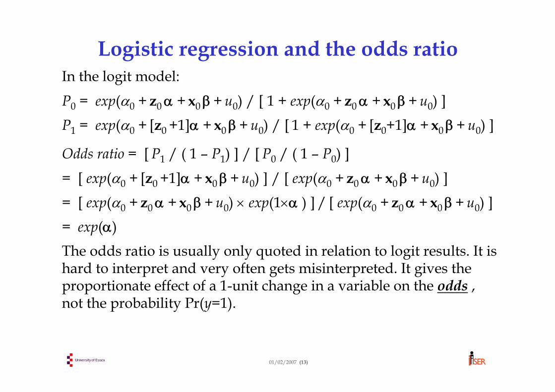
Marginal effects, relative risk and the odds ratioSuppose person 0 has observable characteristics z0 , x0 and unobservable characteristic u0 ; then:

P0 = F(α0 + z0α + x0 β + u0) Let’s consider the effect of making a 1-unit change in (say) z. This means inventing a new person with characteristics:(z0+1 , x0 , u0), for whom Pr(y=1) is:

P1= F(α0 + [z0+1]α + x0 β + u0)We can summarise the effect of this change in various ways:

Marginal effect = P1 – P0

Relative risk = P1 / P0

Odds ratio = [ P1 / ( 1 – P1) ] / [ P0 / ( 1 – P0) ]= [ P1 / P0 ] × [( 1 – P0) /( 1 – P1) ]

Other variables are “held constant” at their baseline values(x0 , u0)

01/02/2007 (13)

Logistic regression and the odds ratioIn the logit model:

P0 = exp(α0 + z0α + x0 β+ u0) / [ 1 + exp(α0 + z0α + x0 β+ u0) ]P1 = exp(α0 + [z0 +1]α + x0 β+ u0) / [ 1 + exp(α0 + [z0+1]α + x0 β+ u0) ]

Odds ratio = [ P1 / ( 1 – P1) ] / [ P0 / ( 1 – P0) ]

= [ exp(α0 + [z0 +1]α + x0 β+ u0) ] / [ exp(α0 + z0α + x0 β+ u0) ]= [ exp(α0 + z0α + x0 β+ u0) × exp(1×α ) ] / [ exp(α0 + z0α + x0 β+ u0) ]= exp(α)The odds ratio is usually only quoted in relation to logit results. It is hard to interpret and very often gets misinterpreted. It gives the proportionate effect of a 1-unit change in a variable on the odds , not the probability Pr(y=1).

01/02/2007 (14)

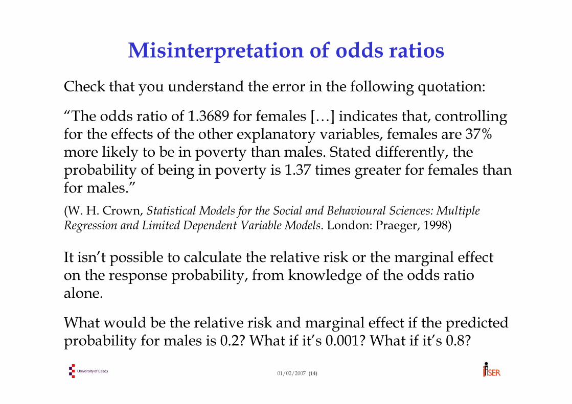
Misinterpretation of odds ratiosCheck that you understand the error in the following quotation:

“The odds ratio of 1.3689 for females […] indicates that, controlling for the effects of the other explanatory variables, females are 37% more likely to be in poverty than males. Stated differently, theprobability of being in poverty is 1.37 times greater for females than for males.”(W. H. Crown, Statistical Models for the Social and Behavioural Sciences: Multiple Regression and Limited Dependent Variable Models. London: Praeger, 1998)

It isn’t possible to calculate the relative risk or the marginal effecton the response probability, from knowledge of the odds ratio alone.

What would be the relative risk and marginal effect if the predicted probability for males is 0.2? What if it’s 0.001? What if it’s 0.8?

01/02/2007 (15)

Options for presentation of results • Present marginal effects evaluated at sample mean values of x

and z, with individual effects u set at zero (i.e. the average in the population). But:

This represents a synthetic, hybrid person that doesn’t exist.Technically, no-one has a zero individual effect (prob is zero)

• Present average partial effects (APE) which allow for the average effect of the unobserved individual effects. Evaluate at:

Mean x and z, or Selected x and z to represent typical person, orEach person’s x and z, and then average the results.

01/02/2007 (16)

Other options for presentation of results • Present predicted probabilities for different

combinations of x and z (representing different types of person). Can also evaluate at different values of the individual effect u, based on its estimated distribution.

• All these methods are difficult with the fixed-effectslogit, as we don’t estimate the (distribution of) individual effects or the coefficients of time-invariant variables.

• Researcher should decide how to present results based on research question being asked.

01/02/2007 (17)

Fixed effects models – some issues

• To deal with individual effects in linear FE models, we can:

estimate individual effects ui (LSDV). difference out individual effects ui .

Estimates of β are unaffected in both cases and are unbiased

• But in non-linear FE models:There’s no short-cut method of calculating the estimator without calculating the estimates of the ui ⇒ the “incidental parameters problem”Estimated coefficients are biasedCan’t remove the individual effects ui by simple differencing as in within-group regression

01/02/2007 (18)

Conditional ML estimation

• CML (as applied here) is a way of condensing the likelihood function into a form which does not depend on ui but does depend on β.

• Then CML is consistent (loosely speaking, unbiased in a large sample) for β.

• But CML is very model specific as it is based on a technical “trick” that is only applicable in a few cases, e.g.:

logit modelsPoisson model (for count data) – see later

• Details of conditional logit are given in the Technical Appendix

01/02/2007 (19)

Fixed effects (or conditional) logitModel: Pr(yit = 1) = F(α0 + zi α + xit β + ui) ,where F( . ) is the logistic form

Avoiding technicalities, the method works as follows:• Work with the subsample of individuals for whom there is some

change in yit during the observation period ⇒ so we sacrifice information on any individuals displaying no change in y

• The changes in the covariates xit (i.e. variable differences like xit -xit) are then used in a modified logit analysis to explain the changes in the observed sequence of outcomes yi1 … yiT .

• Note that differencing the covariates removes any variables thatare constant over time (e.g. gender, birth year, etc.), so α can’t be estimated

• But it also removes ui , so we don’t have to assume anything about ui ⇒ so FE logit is more robust than RE logit

01/02/2007 (20)

Random effects logit/probit

Appropriate if we want to:• estimate the coefficients of zi

• use a non-logistic form • allow for dynamic adjustment (i.e. use the lagged value yit-1 as an explanatory variable)then conditional likelihood is not available. The random effects approach is a natural solution.

[and, of course, RE is preferred if the individual effects are independent of the x – use a Hausman test to decide]

01/02/2007 (21)

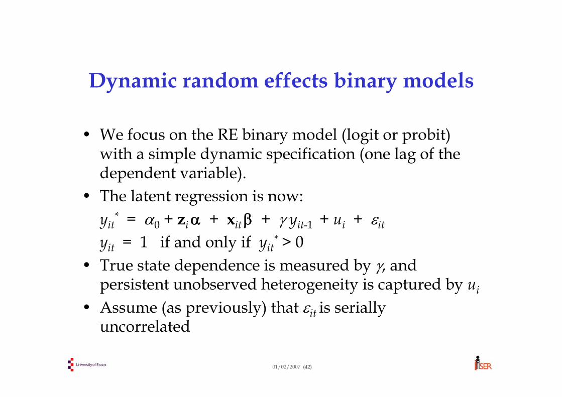
Random effects logit/probitConsider the basic model:

yit* = α0 + ziα + xit β + ui + εit


Make standard random effects assumptions (including independence of (zi , xit ) and ui ).

Since the εit are independent, the joint probability of observing (yi1, yi1,…, yiTi) conditional on ui (and zi , xit ) is just the product of the conditional probabilities for each time period:

Pr(yi1 , ... , yiT | ui ) = Pr(yi1 | ui ) × ... × Pr( yiT | ui )= F(α0+zi α + xi1 β + ui ) × ... × F(α0+zi α + xiT β + ui )

01/02/2007 (22)

Random effects logit/probitMake an assumption about the distribution of ui (usually assumed to be N(0, σu

2)

Average out (marginalise with respect to) the unobservable ui to get the unconditional probability of the data for individual i :

Pr(yi1 , ... , yiT ) = E [ Pr(yi1 , ... , yiT | ui ) ]where “E[ . ]” refers to the expectation or mean with respect to the N(0, σu

2) distribution of ui .

This unconditional probability Pr(yi1 , ... , yiT ) is the likelihood for individual i. Repeated this for all individuals in the sample.

We then choose as our ML estimates the parameter values that maximise the likelihood over the whole sample. This is implemented in Stata, but computing run times are quite long.

This ML method works well only if cov(ui , [zi , xit]) = 0

01/02/2007 (23)

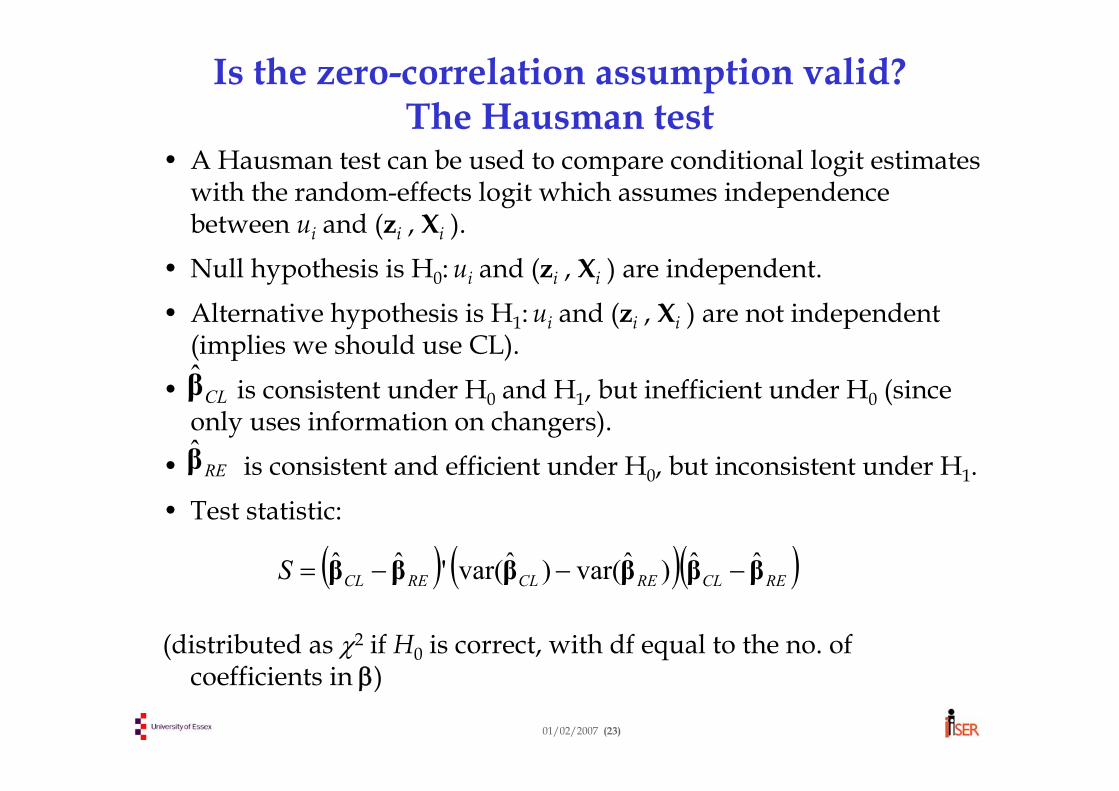
Is the zero-correlation assumption valid? The Hausman test

• A Hausman test can be used to compare conditional logit estimates with the random-effects logit which assumes independence between ui and (zi , Xi ).

• Null hypothesis is H0: ui and (zi , Xi ) are independent.• Alternative hypothesis is H1: ui and (zi , Xi ) are not independent

(implies we should use CL).• is consistent under H0 and H1, but inefficient under H0 (since

only uses information on changers).• is consistent and efficient under H0, but inconsistent under H1.• Test statistic:

(distributed as χ2 if H0 is correct, with df equal to the no. of coefficients in β)

CLβ

REβ

( ) ( )( )RECLRECLRECLS ββββββ ˆˆ)ˆvar()ˆvar('ˆˆ −−−=

01/02/2007 (24)

Individual effects correlated with regressors (1)

• The RE probit/logit assumes that (zi , xit ) and ui are independent.

• Is there any way of relaxing the independence assumption?

• One possibility is to allow ui to be correlated with elements of xit.

A very general formulation (due to Chamberlain) models uias a function of all values of xit from all time periods. A simplified version (based on the Mundlak model) is to model ui as a function of individual means.

01/02/2007 (25)


Using the Mundlak-style approach we have:∼ N(0, ση2) (1)

This formulation still assumes that zi is not correlated with ui. If it is, it belongs in (1), and we can’t separate its correlation with ui from its true effect. Related to this, μabsorbs the main regression constant α0. [Can’t have two constants!]

iiiiiu xx | whereηηδμ ++=

01/02/2007 (26)


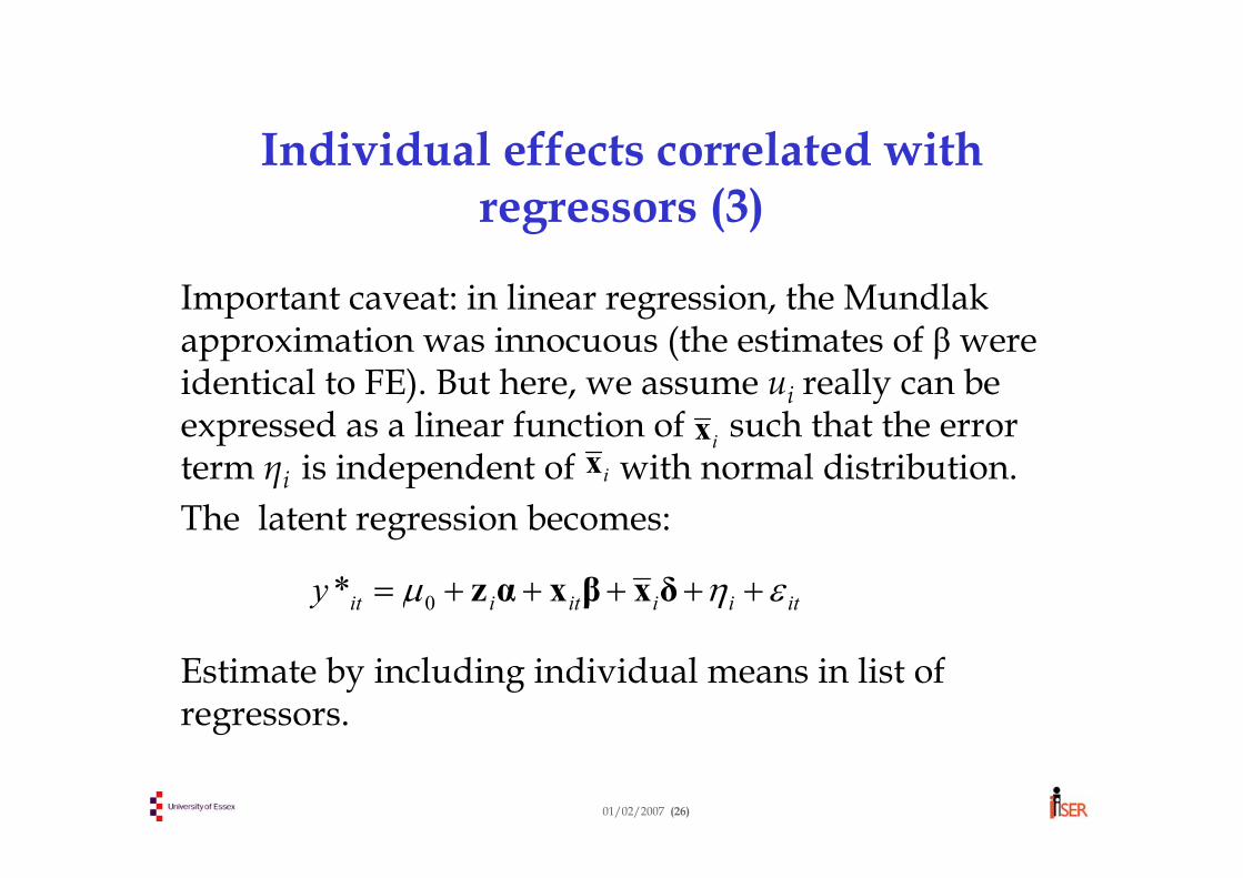
Important caveat: in linear regression, the Mundlakapproximation was innocuous (the estimates of β were identical to FE). But here, we assume ui really can be expressed as a linear function of such that the error term ηi is independent of with normal distribution. The latent regression becomes:

Estimate by including individual means in list of regressors.

ix

itiiitiity εημ +++++= δxβxαz0*

ix

01/02/2007 (27)

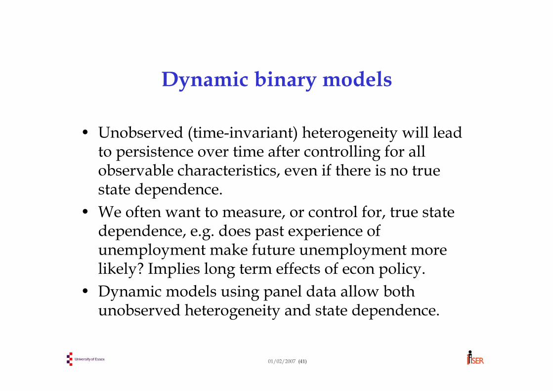
Unobserved heterogeneity or state dependence?• As seen in our data set, there is much persistence in and

repetition of categorical states. Past experience of a given state is often a good predictor of future experience of that state.

• Example: people who were unemployed in the past are more likely to be unemployed in the future.

• There are two possible mechanisms behind this persistence:

State dependence: experience of a given state alters behaviour in the future so as to make that state more likely to occur [see the appendix for dynamic random effects models]Unobserved heterogeneity: individuals differ in their propensity to be in a given state and the factors explaining these differences persist over time and are unmeasured.

01/02/2007 (28)

Technical appendix

The following slides can be safely ignored if you’re not interested in technical detail or if you aren’t familiar with maximum likelihood and the maths of the logit model

Marginal effectsConditional logitRandom effects likelihood functionDynamic random effects model

01/02/2007 (29)

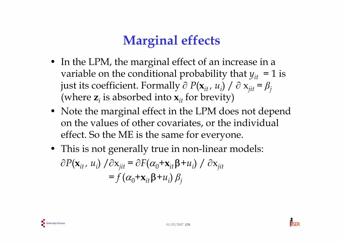
Marginal effects • In the LPM, the marginal effect of an increase in a

variable on the conditional probability that yit = 1 is just its coefficient. Formally ∂ P(xit , ui) / ∂ xjit = βj(where zi is absorbed into xit for brevity)

• Note the marginal effect in the LPM does not depend on the values of other covariates, or the individual effect. So the ME is the same for everyone.

• This is not generally true in non-linear models:∂P(xit , ui) /∂xjit = ∂F(α0+xit β+ui) / ∂xjit

= f (α0+xit β+ui) βj

01/02/2007 (30)

Marginal effects (2)

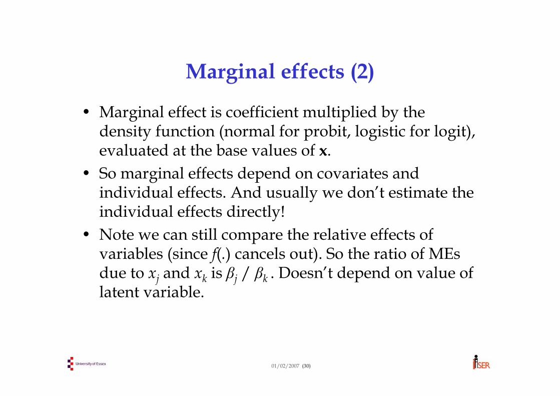
• Marginal effect is coefficient multiplied by the density function (normal for probit, logistic for logit), evaluated at the base values of x.

• So marginal effects depend on covariates and individual effects. And usually we don’t estimate the individual effects directly!

• Note we can still compare the relative effects of variables (since f(.) cancels out). So the ratio of MEsdue to xj and xk is βj / βk . Doesn’t depend on value of latent variable.

01/02/2007 (31)

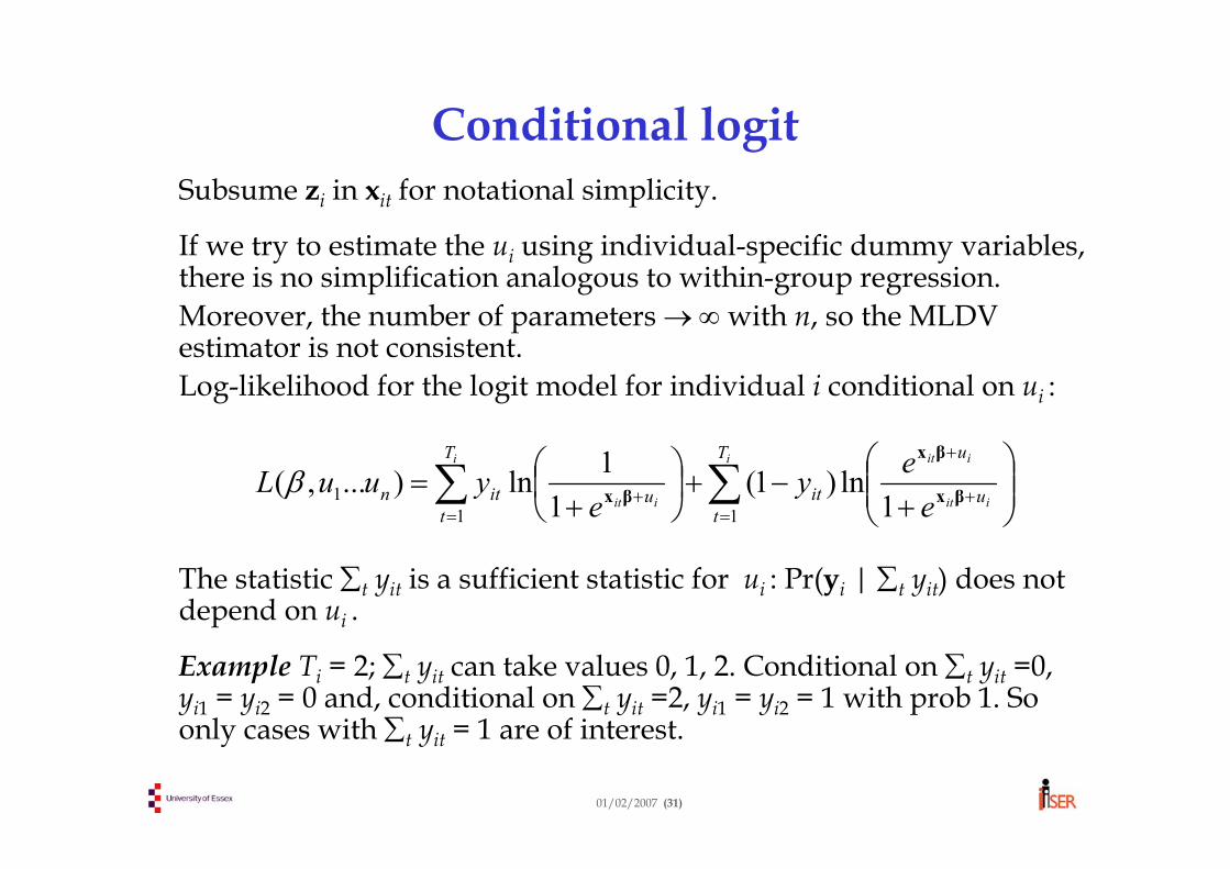
Conditional logitSubsume zi in xit for notational simplicity.

If we try to estimate the ui using individual-specific dummy variables, there is no simplification analogous to within-group regression.Moreover, the number of parameters →∞ with n, so the MLDV estimator is not consistent.Log-likelihood for the logit model for individual i conditional on ui :

The statistic ∑t yit is a sufficient statistic for ui : Pr(yi | ∑t yit) does not depend on ui .

Example Ti = 2; ∑t yit can take values 0, 1, 2. Conditional on ∑t yit =0, yi1 = yi2 = 0 and, conditional on ∑t yit =2, yi1 = yi2 = 1 with prob 1. So only cases with ∑t yit = 1 are of interest.

∑∑=

+

+

=+ ⎟⎟

⎠

⎞⎜⎜⎝

⎛+

−+⎟⎠⎞

⎜⎝⎛+

=i

iit

iiti

iit

T

tu

u

it

T

tuitn e

eye

yuuL11

1 1ln)1(

11ln)...,( βx

βx

βxβ

01/02/2007 (32)

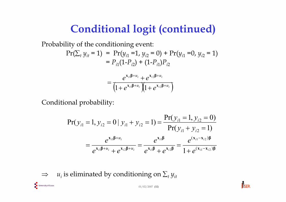
Conditional logit (continued)Probability of the conditioning event:

Pr(∑t yit = 1) = Pr(yi1 =1, yi2 = 0) + Pr(yi1 =0, yi2 = 1)= Pi1(1-Pi2) + (1-Pi1)Pi2

Conditional probability:

⇒ ui is eliminated by conditioning on ∑t yit

( )( )iiii

iiii

uu

uu

eeee

++

++

+++

= βxβx

βxβx

21

21

11

βxx

βxx

βxβx

βx

βxβx

βx

)(

)(21

212121

21

21

21

1

21

1

1

)1Pr()0,1Pr()1|0,1Pr(

ii

ii

ii

i

iiii

ii

ee

eee

eee

yyyyyyyy

uu

uii

iiiiii

−

−

++

+

+=

+=

+=

=+==

==+==

01/02/2007 (33)

Conditional logit (continued)

With T = 2, the conditional log-likelihood is:

where di = 1 if yi1 =1, yi2 = 0 and 0 if yi1 =0, yi2 = 1.

Note that, if xit contains time-invariant covariates (i.e. zi), these disappear from (xi1-xi2) ⇒ α cannot be estimated.

In general, conditional logit only uses data from individuals who experience change in yit over time. This sacrifices sample variation.

•The same conditioning approach does not work with probit and other functional forms, nor with general dynamic models •But it can be generalised to:

unordered multinomial logit models ordered logit models with more than two outcomes.

( )( )∑=Σ

−+−−=1:

)(21

211ln)()(yi

iiiiiedL βxxβxxβ

01/02/2007 (34)

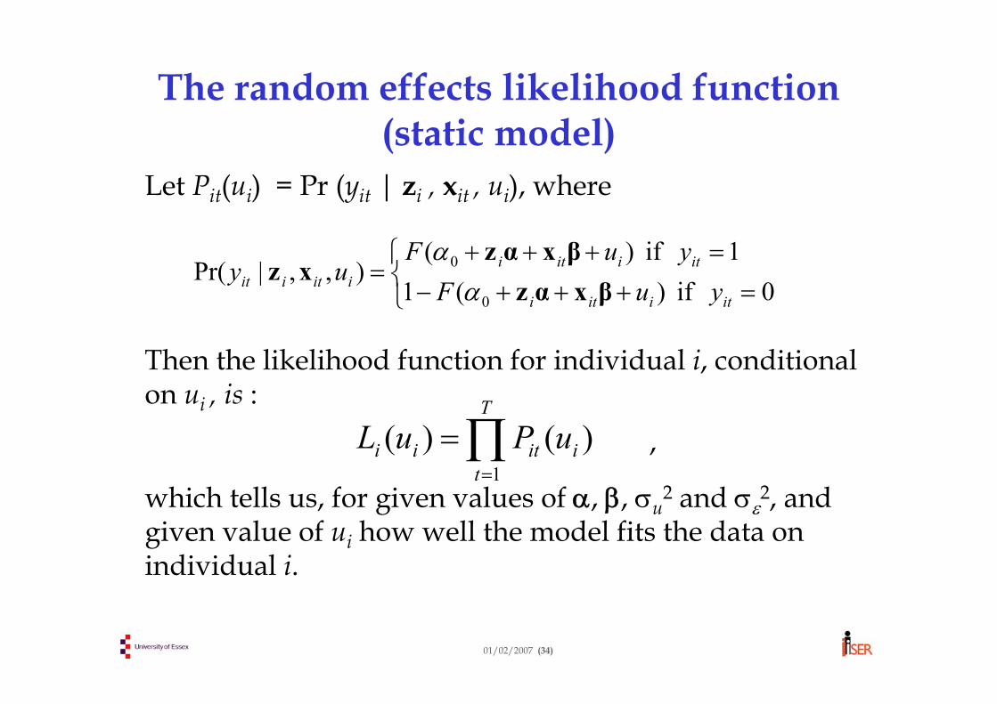
The random effects likelihood function (static model)

Let Pit(ui) = Pr (yit | zi , xit , ui), where

Then the likelihood function for individual i, conditional on ui , is :

,

which tells us, for given values of α, β, σu2 and σε

2, and given value of ui how well the model fits the data on individual i.

⎩⎨⎧

=+++−=+++

=0 if )(1

1 if )(),,|Pr(

0

0

itiiti

itiitiiitiit yuF

yuFuy

βxαzβxαz

xzα

α

∏=

=T

tiitii uPuL

1

)()(

01/02/2007 (35)

Integrating out the random effectsIncluding ui in the conditioning set greatly simplifies the likelihood function, because errors from different time periods are then independent (otherwise, we’d need to allow for dependence across periods).But… we don’t know ui (also we have the incidental parameters problem). We do, however, know (by assumption!) its distribution. Therefore we can “average out ” or marginalise with respect to ui:

where g(u) is an assumed density for u, e.g. for probit, Gaussian: g(u) = σu

-1φ(u/σu). The full likelihood function is L = Π Li

Evaluation of the likelihood function requires the integral to be approximated numerically by a quadrature algorithm.

∫∏∏∞

∞− ==

=⎟⎟⎠

⎞⎜⎜⎝

⎛= duuguPuPEL

ii T

tit

T

tiiti )()()(

11

01/02/2007 (1)

Day 5: Further topics

• Ordered response models• Incomplete panels and sample selection in panel data

models• Dynamic fixed-effects regression models• Dynamic binary logit/probit models• Policy evaluation and panel data• Count data models

01/02/2007 (2)

Topic 1:

Ordered response models

01/02/2007 (3)

Ordered response models

• Ordered (or ordinal) variables take discrete values which have a natural ordering:

Happiness on a scale of 1-5Not working, part-time, full-timeWant fewer, same, more work hoursNo, part, full insuranceCredit rating

• Variables are ordinal but not (necessarily) cardinal, i.e. the “distance” between two categories has no meaning in the model. Only order matters.

01/02/2007 (4)

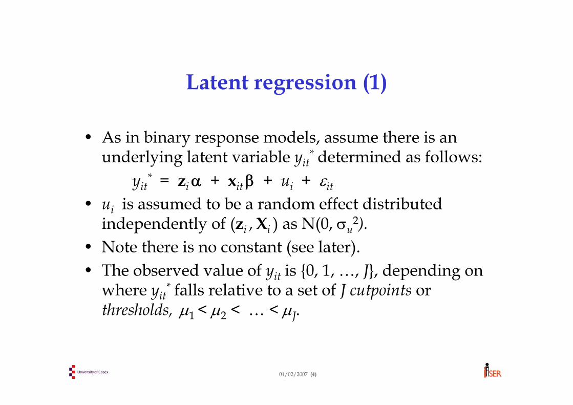
Latent regression (1)

• As in binary response models, assume there is an underlying latent variable yit

* determined as follows:yit

* = ziα + xit β + ui + εit

• ui is assumed to be a random effect distributed independently of (zi , Xi ) as N(0, σu

2).• Note there is no constant (see later).• The observed value of yit is 0, 1, …, J, depending on

where yit* falls relative to a set of J cutpoints or

thresholds, μ1 < μ2 < … < μJ.

01/02/2007 (5)

Latent regression (2)• The outcome yit is given as:

yit = 0 if yit* ≤ μ1

yit = 1 if μ1 < yit* ≤ μ2

.yit = J if μJ < yit

*

• So, if J = 3, there are 2 cutpoints, μ1 and μ2.• And if J = 2 (binary choice model), there is only one

cutpoint, μ1. This is slightly different to the usual specification of the binary probit/logit. Usually, μ1 is normalised to zero and a constant included in the list of regressors. Here, we set the constant to zero and estimate μ1, as is done in Stata’soprobit and reoprob. The choice is arbitrary.

01/02/2007 (6)

Random effects ordered probit (1)• Assume εit is normally distributed with unit variance.Pr(yit = 0 | zi , xit , ui) = Pr(yit

* ≤ μ1 | zi , xit , ui) = Pr (ziα + xit β + ui + εit ≤ μ1)= Φ(μ1 - ziα - xit β - ui)

Pr(yit = 1 | zi , xit , ui) = Pr(μ1 < yit* ≤ μ2 | zi , xit , ui)

= Pr (μ1 < ziα + xit β + ui + εit ≤ μ2)= Φ(μ2 - ziα - xit β - ui) - Φ(μ1 - ziα - xit β - ui)

[which is just Pr (yit* ≤ μ2) minus Pr (yit

* ≤ μ1)]Etc…

01/02/2007 (7)

Random effects ordered probit (2)• Finally:Pr(yit = J | zi , xit , ui) = Pr(μJ < yit

* | zi , xit , ui) = 1 - Pr(yit

* ≤ μJ | zi , xit , ui) = 1- Φ(μJ - ziα - xit β - ui)

• Check that these probabilities sum to one!• Predicting probabilities and calculating marginal

effects is done analogously to the binary RE probit.• But there is a complication in the intermediate

categories 1, … J.

01/02/2007 (8)

Marginal effects• For example (absorb zi into xit for brevity):

Pr(yit=1|xit ,ui) = Φ(μ2 - xitβ - ui) - Φ(μ1 - xitβ - ui)

• So the marginal effect of xjit on the probability that yit=1 is:∂ Pr(yit=1|xit ,ui)/∂xjit = -βjφ(μ2 - xitβ - ui) + βjφ(μ1 - xitβ - ui)

• This can be either negative or positive (consider the φ(.) function). And in general, the sign will vary with xit and ui.

Intuitively, why does the marginal effect have an ambiguous sign?

01/02/2007 (9)

Topic 2:

Incomplete panels and sample selection in panel data models

01/02/2007 (10)

Incomplete panels• We have distinguished between balanced,

unbalanced and non-compact panels. • Most techniques (Stata commands) can be used with

all three types of panel.• But…

We have implicitly assumed that missing observations only represent an efficiency loss (i.e. estimates are still unbiased).In fact, the pattern of missing observations may not be random.If observations are not missing at random, estimates may be biased. Thus unbalanced and non-compact panels may not be random samples. Equally, balanced (sub-)panels may not be random –respondents present at every wave are unlikely to be representative of the population.

01/02/2007 (11)

Non-response• Why might observations be missing?• Unit non-response

Attrition – respondents drop out of panelWave non-response - unavailable at particular waves

• Item non-response Respondents fail to answer particular questions, e.g. income.

• Types of missing-ness:Missing completely at random (MCAR) Missing at random (MAR): conditional on observables (Xi, zi), response is random. Systematic differences in response are explained by observable characteristics.Informative or non-ignorable non-response: systematic differences in response remain after controlling for (Xi, zi).

01/02/2007 (12)

Implications of incompleteness• Implications depend on type of analysis (but this is a

complex area with disagreements between econometricians and survey statisticians).

• Descriptive (i.e. unconditional) statistics will be unbiased if data are MCAR, but biased if data are MAR or non-response is informative.

Example: if poor households are less likely to participate in surveys, we will underestimate the poverty rate.

• Conditional estimates (regressions) are unbiased if data are MCAR or MAR (conditional on observables in model). Biased if non-response is informative.

01/02/2007 (13)

Weights?• Data sets usually include weights which account for:

systematic non-response (as a function of particular observables);non-representative sampling due to survey design.

• Use weights for descriptive stats (if want to make inferences about the population).

• Weighting is more problematic in regression analysis: General purpose weighting model may not be appropriate for a specific regression modelMay be identification problems if same variables used for weights and in regression.Weighting is not necessary if data are MAR, and inflates SEs.In practice, Stata does not accept weights for linear FE and RE (GLS) analysis.

01/02/2007 (14)

Non-random selection in panels

• In the regression framework, non-random response can be represented as follows. Let the model of interest be:yit = ziα + xit β + ui + εit, t = 1 … T , i = 1 … n

• Define a response indicator rit which equals 1 if (yit, zi, xit) is observed in the panel and 0 otherwise.

• If data are MCAR or MAR, then rit is independent of ui and εit.

• If non-response is non-ignorable then rit is not independent of ui and εit. Also called non-random selection or selection on unobservables.

01/02/2007 (15)

Consequences for RE estimates

• We focus on the implications of missing observations for linear RE and FE estimates.

• RE is unbiased if:E(ui +εit |Xi , zi , ri) = E(ui + εit | Xi , zi) = 0where ri = (ri1, …, riT), a vector of selection outcomes in all periods.This says that the composite error term is unrelated to selection conditioning on observable characteristics (MAR or selection on observables).

01/02/2007 (16)

Consequences for FE estimates

• Unsurprisingly (why?), FE is more robust to non-random selection into the panel.

• FE is consistent if:E(εit |Xi , zi, ui , ri) = E(εit | Xi , zi, ui) = 0This says that the transitory error term is unrelated to selection, conditioning on observable characteristics and the individual effect ui. But ri can be related to ui.

• As long as selection into the panel works through “levels”, i.e. time-invariant factors, then FE remains consistent.

01/02/2007 (17)

Testing for non-random selection in panels

• Some simple indicative tests for non-random selection involve:1. checking whether ri helps explain the outcome yit after controlling

for other characteristics2. comparing results from the unbalanced panel with the balanced

sub-panel.

• In the first type of test, functions of rit can be added to the equation and their significance tested [note rit can’t be added –why not?]. For example:

lagged response indicator rit-1

indicator for present in all waves, ci = Π rit

number of waves present for, Ti = Σ rit

The last two can only be used with RE (why?).

01/02/2007 (18)

“Hausman” test2. A second test compares RE or FE estimates from the

unbalanced panel and its balanced sub-panel. If selection is random, the two estimates should be close. If selection is non-random, and affects the estimators differently, we expect a statistically significant difference between the two.For example, test the RE estimator by forming the statistic:

[Not a true Hausman test because neither estimator is consistent in presence of selection bias, and both may be affected similarly by selection. Thus the test may have low “power”]

If these tests suggest attrition bias, the situation is difficult: methods to correct for “endogenous” attrition are complicated

( ) ( ) ( )[ ] ( )biasselection no:under )(~

ˆˆˆvarˆvar'ˆˆ

02

,,

1

,,,,

HkUREBREUREBREUREBRE

χ

ββββββ −−−−

BREURE ,,ˆ and ˆ ββ

01/02/2007 (19)

Topic 3:

Dynamic fixed-effects regression models

01/02/2007 (20)

Dynamic models

Why model dynamics?• Current outcomes might depend on past values of

determinants include lagged xs (distributed lag model). Use similar techniques to those already discussed.

• Adjustment might be partial: this year’s outcome ydepends not only on x, but also on last year’s outcome include lagged y. We will focus on this case.

Notice (as we will see) that this amounts to including an infinite (or back to start of process) number of lagged x.

01/02/2007 (21)

Dynamic models for continuous dependent variables

Adjustment may be imperfect – how to model it? Any conventional time-series model can be used, e.g. AR(1):

yit = ziα + xit β + γ yit-1 + ui + εit (1)

or static model with AR(1) errors:yit = ziα + xit β + ui + εit (2)εit = ρ εit-1 + ηit

⇒ yit = zi (1-ρ)α + (xit -ρ xit-1)β + ρ yit-1 + ui + ηit (2’)NB: model (1) implies gradual adjustment to change in x; model (2) implies a full immediate response.

More general distributed lag models can be used (e.g. ECMs, ARMA, etc.)

01/02/2007 (22)

Within-group estimationWithin-group transformed model (e.g. AR(1)):

where:

NB we assume a compact panel (why?) and an observable initial condition yi0

We have got rid of the individual effect. But what are the statistical properties of a regression of

?

iitiitiitiit yyyy εεγ −+−+−=− − )()( *1βxx

i

T

tit

i

T

tit

ii yy

Ty

Ty

ii

≠== ∑∑−

==−

1

011

* 11

)( and )(on *1 iitiitiit yyyy −−− −xx

01/02/2007 (23)

Properties of the within-group estimator (1)Find an expression for yit that only involves z, x, and yi0 (the starting value or “initial condition” of y).

yit = ziα + xit β + γ yit-1 + ui + εit

By substitution:yit = ziα + xit β +γ (ziα+xit-1 β+γ yit-2+ui+εit-1) + ui + εit

= (1+γ) ziα + xit β +γ xit-1 β + γ2 yit-2+ ui + γui + γεit-1 + εit

= (1+γ) ziα + xit β +γ xit-1 β + γ2(zi α+xit-2 β+γ yit-3+ui+εit-2)+ ui + γui + γεit-1 + εit

= (1+γ+γ2) ziα + xit β +γ xit-1 β + γ2xit-2 β +γ3 yit-3

+ ui + γui + γ2 ui + εit + γεit-1 + γ2εit-2

And so on… Eventually we arrive at t=0.

01/02/2007 (24)

Properties of the within-group estimator (2)Distributed lag form of (1):

⇒ yit-1 is a function of εit-1 … εi1

⇒ is a function of εiT-1 … εi1 and yi0

⇒ is correlated with ⇒ bias in within-group regression coefficients

( )

( ) [ ] 011

1

0

1

0

...11

it

it

itits

sits

ii

t

it

stisiti

t

s

sit

yu

yuy

γεγγεεγγγ

γεγ

+++++++−−

=

++++=

−−−

−−

−

=

∑

∑

βxαz

βxαz

i

T

titi Tyy

i

∑−

=

=1

0

*

*1 iit yy −− iit εε −

01/02/2007 (25)

Properties of the within-group estimator (3)

• Bias of the within-groups estimator is caused by eliminating the individual effect ui from the equation. This causes a correlation between the transformed error term and the transformed lagged dep var.

• Bias is generally negative for small T (even if true γ is zero).

• For large T, bias is small – but with panel data T is not usually large…

What about pooled OLS?

01/02/2007 (26)

Properties of the pooled OLS estimator• Assume individual effects ui are random. In a static

model, OLS is unbiased and consistent (though, recall, inefficient).

• But this is not the case in a dynamic model:yit = ziα + xit β + γ yit-1 + ui + εit

• We know from above that yit-1 is a function of ui and yi0. In general, correlation between yit-1 and ui + εit is positive due to:

Positive contribution from ui.Positive contribution from yi0 if yi0 generated by same process as any other yit

• So OLS is biased upward and is inconsistent

01/02/2007 (27)

Other estimators?

• GLS and ML estimators are also generally biasedThey depend critically on assumptions about initial conditions yi0, and how they are generated

• There are several IV estimators which correct for endogeneity of the lagged dependent variable and are also independent of initial conditions. Like HT, instruments come from inside the model.

Anderson-HsiaoArellano-BondBlundell-Bond…

01/02/2007 (28)

A simple IV estimatorThe within-group transform complicates estimation with lagged endogenous variables. Consider time-differencing:

(1)

The problem now is that the error term, Δεit = εit - εit-1 is a MA(1) process which contains εit-1 , which is correlated with Δyit-1 .⇒ Find a set of instruments correlated with Δyit-1 but uncorrelated with εit-1

⇒ All lagged xit and yit-2 … yi0 are valid instruments if εit is serially independent⇒ Simplest IV estimator (Anderson Hsiao) estimates (1), using instruments (xit, xit-1, xit-2,yit-2).⇒ We can only use observations t = 2 … Ti . Each extra lag used as an instrument loses us n observations.⇒ Once is found, estimate α by regressing on zi

iitititit Ttyy ...2,ΔΔΔ 1 =++=Δ − εγβx

IVβ IViiy βx ˆ−

01/02/2007 (29)

Problems with IV estimatorsSuppose yit is a random walk (e.g. Hall’s (1978) form of the permanent income hypothesis: dynamic choice models based on Euler conditions).⇒yit-2 is uncorrelated with Δyit-1 and is not a valid instrument⇒IV methods based on a differenced model won’t work well if there is a near-unit root

Any method based solely on the differenced equation ignores potentially valuable information contained in the initial condition yi0

What is the optimal point on the trade-off between the number of lags used as instruments and the number of time periods retained in the estimation sample?

01/02/2007 (30)

System estimatorsThe time-differenced model:

(1)

This is a system of Ti-1 linear equations with cross-correlated errors (since Δεit is correlated with Δεit-1 and Δεit+1)

There is also some (related) process generating the initial conditions, yi0 and yi1, which could provide further equations.

A different number of instruments is available for each of the equations in (1):

E.g. the equation for t = 2 has only (xi0 … xiT , yi0);the equation for t = Ti has (xi0…xiT , yi0… yiT-2).

NB it’s assumed here that xi0 is observable

iitiititit Ttuyy ...2,ΔΔΔ 1 =+++=Δ − εγβx

01/02/2007 (31)

Digression: method of moments (1)The method of moments is a way of getting consistent

estimates of model parameters.1. Specify moment conditions (e.g. means, covariances)

implied by the model as a function of its parameters (population moments).

2. Write down the “sample analogues” of these moment conditions, i.e. expressions into which you can plug the sample data, as a function of parameter estimates.

3. Choose values for the parameter estimates which “solve” the sample moment conditions.

01/02/2007 (32)

Digression: method of moments (2)

Very simple example: mean of a random variable y.1. Mean of y is defined as μ = E[y]. Rearrange as a

moment condition: m(y; μ) = E[y - μ] = 0.

2. Sample analogue is

3. Solve to get MM estimator:

( ) ( ) 01;ˆ1

=−= ∑=

n

iiyn

m μμy

∑=

=n

iiyn 1

1μ

01/02/2007 (33)

Digression: method of moments (3)

•Often there are more moment conditions than parameters to be estimated. Then the moment conditions don’t have a unique solution.•In this case, we minimise a (weighted) sum of the squares of the sample moments. In vector notation this is written in the general case as where V is the weighting matrix.•This is called the generalised method of moments (GMM).

),,(ˆ'),,(ˆ 1 βxymVβxym −

01/02/2007 (34)

Generalised method of moments IV estimators are members of the class of GMM estimatorse.g. the 2SLS estimator, is the following M-estimator:

where is the “sample analogue”, n-1Q’(y-Xβ), of a moment, Eq’ε, assumed to be zero in the population.

V is a weighting matrix proportional to the asymptotic covariance matrix of the moment condition (in this standard 2SLS example σε 2Q’Q , where σε 2 is the residual variance).

GMM can be extended to any number of moment conditions

( ) yQQQQXXQQQQXβ ')('')('ˆ 111 −−−= ''IV

m

( ) ( )

),,(ˆ'),,(ˆmin arg

')'('min argˆ

1

1

βxymVβxym

XβyQQQQXβyβ

β

β

−

−

=

−−=IV

01/02/2007 (35)

Arellano-Bond GMM (1991)

m

We have Ti -2 differenced equations (1). The instruments for equation t are:

qit = (xi0…xiT , yi0…yit-2)Full set of moment conditions:

E qi2‘ Δεi2 = 0 (Ti+1)kx+1 conditionsE qi3‘ Δεi3 = 0 (Ti+1)kx+2 conditions

.

.E qiT‘ ΔεiT = 0 (Ti+1)kx+Ti-1 conditions

is a [(Ti +1)(Ti -1)kx +Ti (Ti -1)/2] × 1 moment vectorThe optimal choice for V is More conditions can be added (e.g. for zi and to impose the homoskedasticity assumption on εit). But GMM often works badly in finite samples with many moment conditions.

'ˆˆ iiE mm

01/02/2007 (36)

Specification testing(1) Testing for over-identifying restrictions

The number of restrictions = the number of moment conditions for each individual (r) minus the number of parameters (kx).

Sargan test statistic:The minimized optimal GMM criterion scaled by n is

has an asymptotic chi-square distribution with r- kxdegrees of freedom.

( ))ˆ,,(ˆˆ')ˆ,,(ˆ 1 βxymVβxym −= nS

01/02/2007 (37)

Specification testing(2) Testing for residual serial correlation

If the εit are serially independent, thenE[Δ εit Δ εit-1]=E[(εit - εit-1)(εit -1- εit -2)]=-E[εit -1

2]=-σε 2

Also var(εit - εit-1)=var(εit-1- εit-2)=2 σε 2

Thus, the first order serial correlation coefficient is r1=E[Δ εit Δ εit-1]/[√var(Δεit)√varΔ εit-1)] = 0.5.

But E[Δ εit Δ εit-2]=0, and so the second order serial correlation coefficient r2=0.

⇒ test for second order serial correlation.Specification error if second order serial correlation is

statistically significant.

01/02/2007 (38)

Further developments: initial conditions

Arellano-Bond ignores the initial conditions yi0 and yi1 and only uses moment conditions for Δyi2…ΔyiT .To progress further, we need additional assumptions about the initial conditions. One possibility is:

Equilibrium initial values. If the process is homogeneous and long-established:

⇒Coefficient of ui in equation for yi0 is (1-γ )-1

⇒But the quantity is unobserved⇒Also, do people really have infinite pasts?

If lagged levels of yit are poor instruments for Δyit-1 , can we go back to using the equations in level form?

∑∞

=−

0,

ssi

sxγ

( )∑∞

=−− ++

−+

=0

,,0 1 ssisi

siii

uy εγγ

βxαz

01/02/2007 (39)

Extended system methodsArellano & Bover (1995) and Blundell & Bond (1998) (see also Bhargava & Sargan, 1983) suggested using the model in bothdifferenced and levels form to generate GMM moment conditions.Question: in the levels model

yit = ziα + xit β + γ yit-1 + ui + εit , (1)is there a good instrument for yit-1? This instrument must be uncorrelated with ui as well as εit .

A&B suggested Δyit-1 , etc.. The instrument validity condition is E[Δyit-1 (ui + εit)] = 0, which requires (see B&B, 1998):

E ui [ yi0 – ui/(1-γ )] = 0 (2)E uiΔεit = 0 (3)

(2) Requires yi0 to be in stationary equilibrium. It then improves estimation precision in highly-persistent models (i.e. when γ ≈ 1)

01/02/2007 (40)

Topic 4:

Dynamic binary logit/probit models

01/02/2007 (41)

Dynamic binary models

• Unobserved (time-invariant) heterogeneity will lead to persistence over time after controlling for all observable characteristics, even if there is no true state dependence.

• We often want to measure, or control for, true state dependence, e.g. does past experience of unemployment make future unemployment more likely? Implies long term effects of econ policy.

• Dynamic models using panel data allow both unobserved heterogeneity and state dependence.

01/02/2007 (42)

Dynamic random effects binary models

• We focus on the RE binary model (logit or probit) with a simple dynamic specification (one lag of the dependent variable).

• The latent regression is now:yit

* = α0 + ziα + xit β + γ yit-1 + ui + εit


• True state dependence is measured by γ, and persistent unobserved heterogeneity is captured by ui

• Assume (as previously) that εit is serially uncorrelated

01/02/2007 (43)

The random effects likelihood functionConstruct a likelihood by sequential conditioning:

Pr(yi0 | zi , Xi , ui) = Pi0(ui) Pr(yi1 | yi0 , zi , xi1 , ui) = Pi1(yi0 , ui)

.

.Pr(yiT | yiT-1 , zi , xiT , ui) = PiT(yiT-1 , ui)

The probabilities Pit (for t = 1, …, T) are of the form:F(α0 + ziα + xitβ + γ yit-1 + ui) for yit = 1

or 1 - F(α0 + ziα + xit β + γ yit-1 + ui) for yit = 0.

Likelihood function for individual i, conditional on ui:

∏=

−=iT

tiititiiii uyPuPuL

110 ),()()(

01/02/2007 (44)

Initial conditions• The Pi0(ui) term in the likelihood is the contribution

of the initial condition – the first observed value y. • If yi0 is exogenous (unrelated to the individual effect)

then effectively Pi0(ui) can be dropped from the likelihood

Just condition on yi0 in Pi1(yi0 , ui)Possible efficiency loss since useful information about the starting point may be neglected.

• But yi0 is probably not exogenous:It is probably not the true starting point of the “process”, just the start of our sampleIn any case, yi0 is probably not randomly allocated, but related to ui as are the other yit.

01/02/2007 (45)

Heckman’s method

• In practice, it is difficult to derive an exact expression for Pi0(ui), especially if we do not observe the process from the beginning.

• Heckman (1981) suggested approximating Pi0(ui) by a simple probit model, where regressors can include “pre-sample” information (e.g. family background).

• Can be complicated to estimate.

01/02/2007 (46)

Wooldridge’s methodWooldridge suggested an alternative: condition on yi0, without specifying its probability. Instead, model the density of ui conditional on yi0, xi. This is related to the Chamberlain/Mundlak approach discussed earlier.So ui could be specified as:

and the latent regression is now:

Can be estimated as standard RE probit – include and yi0 every period.Again, though, note this is just an approximation.

) N(0, as ddistribute is ,| where 2000 ησηηγδμ iiiiiii yyu xx +++=

itiiiitiiti yyy εηγδγμ +++++++= − 0010* xαzβx

ix

01/02/2007 (47)

Topic 5:

Policy evaluation and panel data

01/02/2007 (48)

Policy evaluation and panel data

• A specialised application of statistics is to evaluate the impact of various new policies, e.g. training schemes, changes to tax-benefit system, minimum wages.

• Policy evaluation often uses panel data.• We look briefly at the parameters that policy

evaluation methods try to measure and how they relate to panel data estimators seen earlier in the course.

01/02/2007 (49)

Potential outcomes and counterfactuals

• Aim is to evaluate impact of some policy ‘treatment’ (terminology originates in clinical trials).

• Each individual has two potential outcomes, y1i (with treatment) and y0i (without treatment).

• The treatment effect is Δi = yi1 – yi0. Note that Δipotentially differs over individuals (e.g. some people benefit more from training than others).

• Problem is we only observe each individual in one state (treated or untreated). We don’t observe the counterfactual state, i.e. what would have happened to the treated person had they not been treated, and the untreated person had they been treated.

01/02/2007 (50)

Average treatment effects (1)• Say we want to estimate the average effect of the

treatment. The population average treatment effect (ATE) is E(Δi)= E(y1i – y0i) = E(y1i) – E(y0i). But, as already seen, we don’t observe y1i and y0i for all individuals in the sample.

• But, using available observations, we could estimate (naively): E(y1i|di = 1) – E(y0i|di = 0)

= E(y1i|di = 1)–E(y0i|di = 1)+E(y0i|di = 1)–E(y0i|di=0)= E(y1i –y0i|di = 1) + E(y0i|di = 1) – E(y0i|di=0)= ATT + E(y0i|di = 1) – E(y0i|di = 0)where di indicates treatment and ATT is the average effect

of treatment on the treated.

01/02/2007 (51)

Average treatment effects (2)• ATT will often differ from ATE. E.g. training may be

given to those who benefit the most from it. But ATT is often the more relevant parameter for policy purposes – e.g. want to know the impact on those who will actually participate in a scheme.

• The naïve estimator includes a bias/selection term E(y0i|di = 1) – E(y0i|di = 0), which is the difference in untreated outcomes between those who got the treatment and those who didn’t. This term will not be zero if, e.g., trainees would have earned less (or more) than non-trainees even without training.

01/02/2007 (52)

Before-after estimator (1)The bias term highlights the key problem in policy evaluation, which is making sure that the treated and untreated groups are very similar (ideally, identical). On average, the outcomes of the 2 groups should be the same in the absence of the treatment.Consider a possible estimator using two waves of panel data (t and t+1), with treatment occurring after the first wave. Compare treated individuals with their “untreated selves” in the previous wave, i.e. estimate:

E(y1it+1|di = 1) – E(y0it|di = 1) by sindividual dfor treate outcomemean theis where,1

TTt

Tt yyy −+

01/02/2007 (53)

Before-after estimator (2)

• The before-after estimator uses outcomes before treatment (at t) to proxy (non-observed) outcomes at t+1 without the treatment. It identifies ATT on the assumption that E(y0it+1|di = 1) = E(y0it|di = 1)

• However, even without the treatment, outcomes may have changed between t and t+1 because of macro factors or lifecycle effects.

• To control for these trends, we can include a control group who never receive the treatment but (are assumed to) experience the same trends.

01/02/2007 (54)

Difference-in-difference estimatorThe difference-in-difference (DID) estimator takes the difference between the change in outcomes for treated individuals and the change for untreated (control) individuals. DID is estimated as:

A weakness of DID is that the common trend assumption may be violated:

macro trends may affect the 2 groups differentlymay be time-varying factors affecting only one group, e.g.

“Ashenfelter’s dip”: often trainees had a temp drop in earnings before they took up training course.

( ) ( )sindividual (control) dfor treate outcomemean theis )( where

11CT

Ct

Ct

Tt

Tt

yy

yyyy −−− ++

01/02/2007 (55)

RegressionsConsider a regression model with a treatment dummy, time trend and interaction :yit = α0 + γ di + θw2t + ρdi.w2t + ui + εit ,

t = 1, 2; i = 1 … nwhere w2t equals 1 if t=2 and zero otherwise.It is easily shown that in this simple case (2 waves and no other controls) is identical to DID and so identifies ATT. Can estimate as RE, FE (in which case didrops out) or by pooled OLS (adjust SEs).Can add controls xit to account for differing trends -though interpretation of is less straightforward (unless treatment effect same for all, Δi= Δ).

ρ

ρ

01/02/2007 (56)

Other estimators

• Other estimators of treatment effects match treatment and control individuals based on observed characteristics x. A popular estimator of this type is propensity score matching.

• Matching estimators can be less restrictive (don’t assume linear functional form) and allow more flexible analysis of heterogeneous treatment effects.

• But they assume treatment is unrelated to potential outcomes conditional on x: selection on observables.

• Can also combine matching with DID.

01/02/2007 (57)

Topic 6:

Count data models

01/02/2007 (58)

Count data• Quantities are often inherently discreet, or are

measured discreetly. Frequencies are inherently discreet. Examples of count variables:

Number of visits to doctorNumber of organisations joined.Number of arrests.Number of patent applications.

• Counts cannot be negative, may be (are often?) zero and always take integer values.

• Modelling counts as continuous variables would not take account of this “lumpy” distribution (cfproblems with LPM for binary variables).

01/02/2007 (59)

Modelling count data (1)Counts are typically modelled as a Poisson distribution. The probability of individual i experiencing yit events in period t is:

Where does this come from? Imagine a simple experiment that would produce a distribution of counts. We toss a coin n=10 times and count the number of heads (probability p of a head from a toss = 0.5).This would produce a binomial distribution, with mean number of heads = np = 5.

!)exp()Pr(

it

yitit

it yy

itλλ−=

01/02/2007 (60)

Modelling count data (2)

• The Poisson distribution is the limiting form of the binomial distribution as the number of “trials” (tosses) goes to infinity, and p gets correspondingly smaller so as to keep constant the mean count np(=λ).

• The mean of the Poisson distribution is λit.• The variance of the Poisson distribution is also λit

(often rejected in practice!).• Allow for observed and unobserved characteristics

by specifying λit = exp(ziα + xit β + ui). Note the exponential form guarantees λit > 0.

01/02/2007 (61)

Poisson regression

• The Poisson model is usually estimated by maximum likelihood (ML)

• The ML estimator is quite “robust”: provided the conditional mean is correctly specified, the estimates are consistent even if the true distribution is not Poisson.

• The conditional mean is: E(yit | zi, xit, ui) ≡ λit = exp(ziα + xit β + ui)

= exp(ui) . exp(ziα + xit β)

01/02/2007 (62)


• So the individual effect ui affects the conditional mean multiplicatively. This turns out to be convenient.

• Since E(yit | zi, xit, ui) = exp(ui) . exp(ziα + xit β), if xjitincreases by 1 unit, holding all else constant, the ratio of the new to the old mean number of events is exp(βj). In Stata, using the irr option, this is reported as an “incident rate ratio”.

• Notice the IRR is independent of ui.

01/02/2007 (63)


• Alternatively, the marginal effect of xjit on the expected count is:∂ E(yit | zi , xit , ui) /∂xjit = βj exp(ui).exp(ziα + xit β)

= βj E(yit | zi , xit , ui) • Semi-elasticity: a 1 unit increase in xjit has a 100 βj %

effect on the expected count, all else constant.• Equivalently, βj is the marginal effect on the log of

the expected count.

01/02/2007 (64)

Random effects Poisson model

• We still have to deal with ui. In the RE model, we assume that the multiplicative individual effect is independent of (zi , Xi ) and has a gamma distribution with a mean of one (analogous to mean zero in an additive model) and constant variance (=α in Stata).

• Stata also allows a normally distributed individual effect (but runs slower).

01/02/2007 (65)

Fixed effects Poisson model

•The Poisson regression can also be estimated as a fixed effects model, allowing arbritary dependence of ui on (zi, Xi ).•As for the conditional (FE) logit, the method is to condition on a sufficient statistic. The sufficient statistic is the sum for each individual of the observed counts over the panel ( )

•As usual in FE models, the effects (α) of time-invariant variables zi cannot be identified.

∑=

=iT

tity

1

01/02/2007 (66)

Over- (and under-) dispersion• A restrictive feature of the Poisson model is that the

mean and variance of yit are constrained to be the same.

• In practice, the variance is usually greater than the mean – overdispersion. One reason is unobserved heterogeneity (cf linear regression where individual effects increase the variance of the composite error term).

• The negative binomial distribution allows for overdispersion.

• But, with panel data techniques we already allow explicitly for unobserved heterogeneity.

RE incorporates overdispersionFE is consistent in presence of either under- or overdispersion.

Date post:	20-Jun-2018
Category:	Documents
Upload:	trandang
View:	227 times
Download:	1 times

Lectures on: Panel data analysis for social scientists ... · Panel data analysis for social...

Documents