83
Lei Bu Petri Nets 1
| Date post: | 18-Dec-2015 |
| Category: |
Documents |
| Upload: | dwain-benson |
| View: | 224 times |
| Download: | 0 times |

Lei Bu
Petri Nets
1

Dining Philosphier
4 States , 5 transitions

9 States 14 Transitions

27 States , 56 Transitions

81 States , 252 Transitions

• automata are a theoretical and idealised model
• they reflect a Newtonian world-view:• space & time as an absolute frame of reference • clockwork view of processes within this frame
• Carl Adam Petri has made an attempt to combine automata from theoretical CS, and pragmatic expertise from engineers: Petri Net
From automata to Petri Net
• state is distributed, transitions are localised • local causality replaces global time• subsystems interact by explicit communication

Petri nets-Motivation
In contrast to state machines, state transitions in Petri nets are asynchronous. The ordering of transitions is partly uncoordinated; it is specified by a partial order.
Therefore, Petri nets can be used to model concurrent distributed systems.
Many flavors of Petri nets are in use, e.g. Activity charts(UML) Data flow graphs and marked graphs
7

History
1962: C.A. Petri’s dissertation (U. Darmstadt, W. Germany) 1970: Project MAC Conf. on Concurrent Systems and Parallel Computa-
tion (MIT, USA) 1975: Conf. on Petri Nets and related Methods (MIT, USA) 1979: Course on General Net Theory of Processes and Systems (Ham-
burg, W. Germany) 1980: First European Workshop on Applications and Theory of Petri
Nets (Strasbourg, France) 1985: First International Workshop on Timed Petri Nets (Torino, Italy)
Introduction
Petri Nets: Graphical and Mathematical modeling tools graphical tool
visual communication aid mathematical tool
state equations, algebraic equations, etc
concurrent, asynchronous, distributed, parallel, nonde-terministic and/or stochastic systems

Informal Definition
The graphical presentation of a Petri net is a bipartite graph
There are two kinds of nodes Places: usually model resources or partial state of the sys-
tem Transitions: model state transition and synchronization
Arcs are directed and always connect nodes of differ-ent types
Tokens are resources in the places
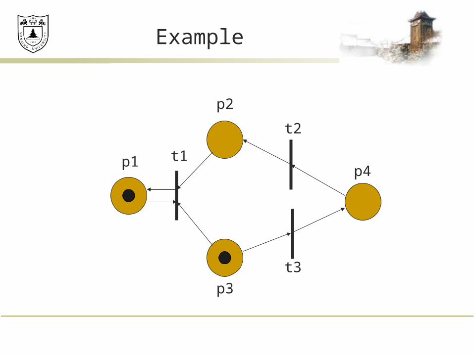
Example
p2
t1p1
t2
p4
t3
p3

Definition of Petri Net
C = ( P, T, I, O) Places
P = { p1, p2, p3, …, pn} Transitions
T = { t1, t2, t3, …, tn} Input
I : T Pr (r = number of places) •t Output
O : T Pq (q = number of places) t •
12

marking µ : assignment of tokens to the places of Petri net µ = µ1, µ2, µ3, … µn
13
p2
t1p1
t2
p4
t3
p3

Applications
performance evaluation communication protocols distributed-software systems distributed-database systems concurrent and parallel programs industrial control systems discrete-events systems multiprocessor memory systems dataflow-computing systems fault-tolerant systems etc, etc, etc

Basics of Petri Nets
Petri net consist two types of nodes: places and transitions. And arc exists only from a place to a transition or from a transition to a place.
A place may have zero or more tokens. Graphically, places, transitions, arcs, and tokens are
represented respectively by: circles, bars, arrows, and dots.
Below is an example Petri net with two places and one transaction.
15
p2 p1
t1

State
The state of the system is modeled by
marking the places with tokens A place can be marked with a finite
number (possibly zero) of tokens

Fire
A transition t is called enabled in a certain marking, if: For every arc from a place p to t, there exists a distinct to-
ken in the marking An enabled transition can fire and result in a new
marking Firing of a transition t in a marking is an atomic op-
eration
state transition of form (1, 0) (0, 1)p1 : input place p2: output place p2 p1
t1

Fire (cont.)
Firing a transition results in two things:1. Subtracting one token from the marking of any place p for
every arc connecting p to t
2. Adding one token to the marking of any place p for every arc connecting t to p
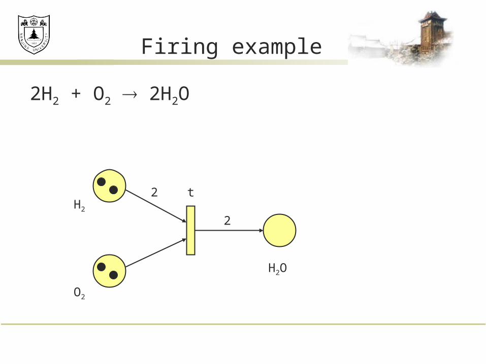
Firing example
2H2 + O2 2H2O
H2
O2
H2O
t
2
2

Firing example
2H2 + O2 2H2O
H2
O2
H2O
t
2
2

Run-1 Safe PN
A run of a Petri net is a finite or infinite sequence of markings and transitions
… …
such that is the initial marking of the net, for any i () , and that
• for any i ()
21
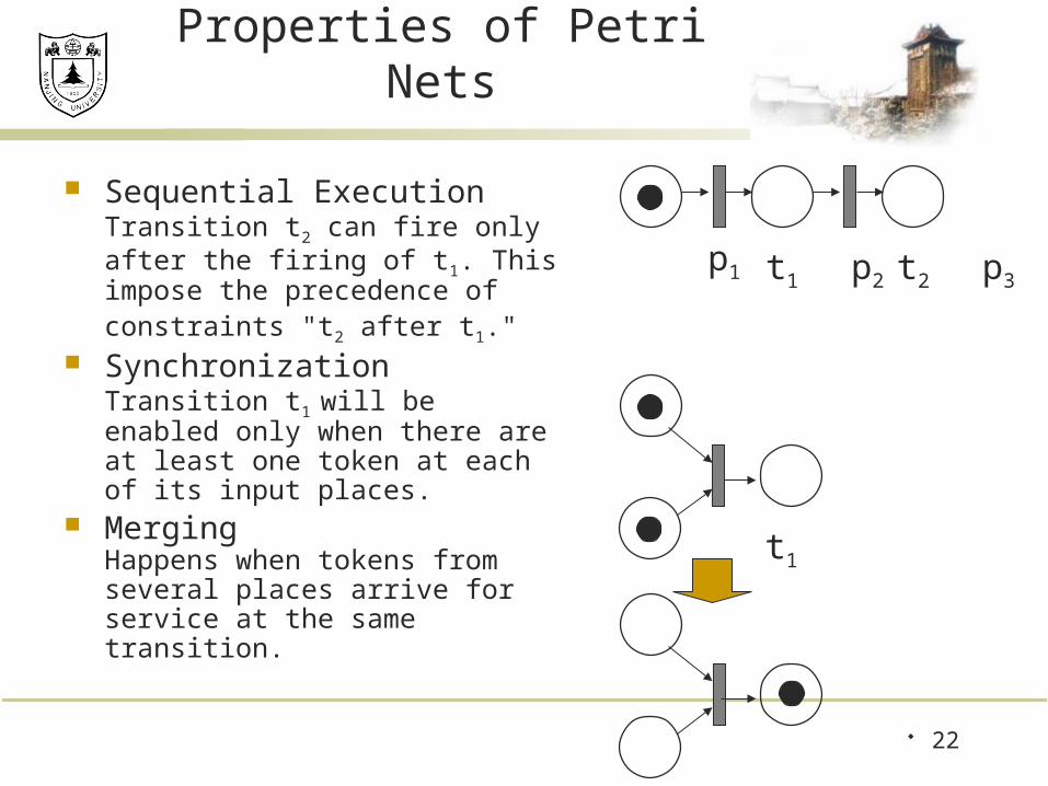
Properties of Petri Nets
Sequential ExecutionTransition t2 can fire only after the firing of t1. This impose the prece-dence of constraints "t2 after t1."
SynchronizationTransition t1 will be enabled only when there are at least one token at each of its input places.
MergingHappens when tokens from several places arrive for service at the same transition.
22
p2
t1
p1 p3
t2
t1

Fork

Properties of Petri Nets -continued
Concurrency t1 and t2 are concurrent. - with this property, Petri net is able to model systems of dis-tributed control with multiple processes executing concur-rently in time.
24
t1
t2

Non-Deterministic Evolution
The evolution of Petri nets is not deterministic
Any of the activated transactions might fire
25
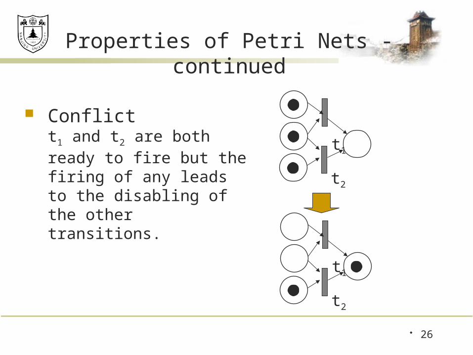
26
Conflictt1 and t2 are both ready to fire but the firing of any leads to the disabling of the other transi-tions.
t1
t2
t1
t2
Properties of Petri Nets -continued

27
Conflict - continued
the resulting conflict may be resolved in a purely non-deterministic way or in a probabilistic way, by assigning appropriate probabilities to the conflicting transitions.
there is a choice of either t1 and t2, or t3 and t4
t1 t2
t3 t4
Properties of Petri Nets -continued

Some definitions
source transition: no inputs sink transition: no outputs self-loop: a pair (p,t) s.t. p is both an input and an output of t pure PN: no self-loops Weighted PN: arcs with weight ordinary PN: all arc weights are 1’s infinite capacity net: places can accommodate an unlimited number of
tokens finite capacity net: each place p has a maximum capacity K(p) strict transition rule: after firing, each output place can’t have more
than K(p) tokens Theorem: every pure finite-capacity net can be transformed into an
equivalent infinite-capacity net
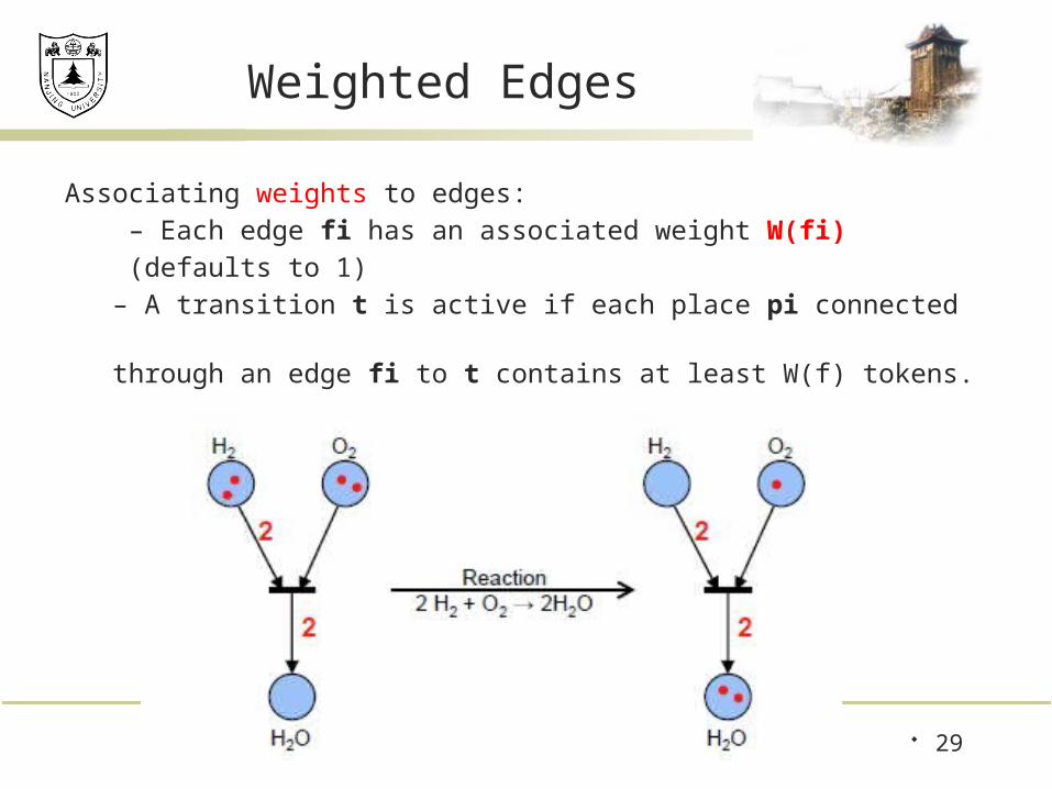
Weighted Edges
Associating weights to edges:
– Each edge fi has an associated weight W(fi)
(defaults to 1)
– A transition t is active if each place pi connected
through an edge fi to t contains at least W(f) tokens.
29

Finite Capacity Petri Net
Each place pi can hold maximally K(pi) tokens A transition t is only active if all output places pi of t cannot ex-
ceed K(pi) after firing t.
Pure finite capacity Petri Nets can be transformed into equiva-lent infinite capacity Petri Nets (without capacity restrictions).
Equivalence: Both nets have the same set of all possible firing sequences
30

Removing Capacity Constraints
For each place p with K(p) > 1, add a complementary place p’ with initial marking M0(p’) = K(p) – M0(p).
For each outgoing edge e = (p, t), add an edge e’ from t to p’ with weight W(e).
For each incoming edge e = (t, p), add an edge e’ from p’ to t with weight W(e).
31

Resolving Self-Loops
The algorithm to remove capacity constraints works if the Petri net has no self loops (is pure).
No Problem! Rewrite the Petri net without self loops:
32
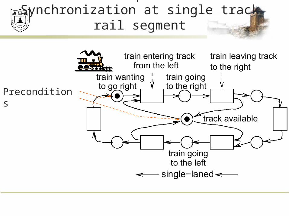
Example: Synchronization at single track rail segment
Preconditions
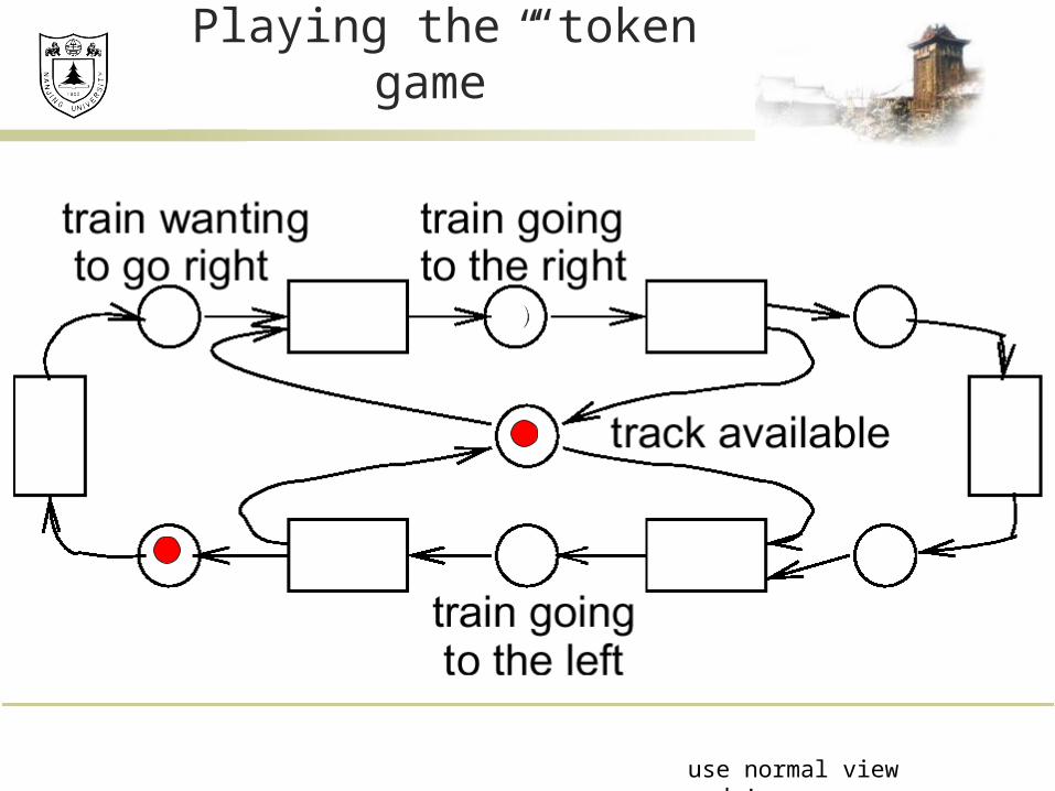
Playing the “token game”
use normal view mode!

Conflict for resource track

Modeling communication protocols
readyto send
waitfor ack.
ack.received
msg.received
ack.sent
readyto receive
bufferfull
bufferfullsend
msg.
receiveack.
receivemsg.
sendack.
proc.1 proc.2
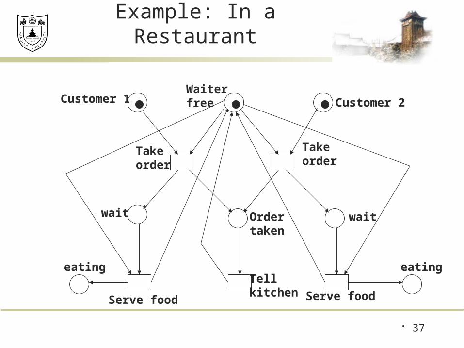
Example: In a Restaurant
37
WaiterfreeCustomer 1 Customer 2
Takeorder
Takeorder
Ordertaken
Tellkitchen
wait wait
Serve food Serve food
eating eating

Example: In a Restaurant (Two Scenarios)
Scenario 1: Waiter takes order from customer 1; serves customer 1;
takes order from customer 2; serves customer 2.
Scenario 2: Waiter takes order from customer 1; takes order from
customer 2; serves customer 2; serves customer 1.
38

Example: In a Restaurant (Scenario 1)
39
WaiterfreeCustomer 1 Customer 2
Takeorder
Takeorder
Ordertaken
Tellkitchen
wait wait
Serve food Serve food
eating eating
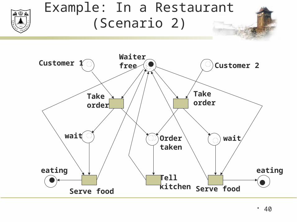
Example: In a Restaurant (Scenario 2)
40
WaiterfreeCustomer 1 Customer 2
Takeorder
Takeorder
Ordertaken
Tellkitchen
wait wait
Serve food Serve food
eating eating

Example: Vending Machine
41
5c
Take 15c bar
Deposit 5c
0c
Deposit 10c
Deposit 5c
10c
Deposit 10c
Deposit5c
Deposit 10c20c
Deposit5c
15c
Take 20c bar

Example: Vending Machine (3 Scenarios)
Scenario 1: Deposit 5c, deposit 5c, deposit 5c, deposit 5c, take 20c
snack bar. Scenario 2:
Deposit 10c, deposit 5c, take 15c snack bar. Scenario 3:
Deposit 5c, deposit 10c, deposit 5c, take 20c snack bar.
42

Example: Vending Machine
43
5c
Take 15c bar
Deposit 5c
0c
Deposit 10c
Deposit 5c
10c
Deposit 10c
Deposit5c
Deposit 10c20c
Deposit5c
15c
Take 20c bar

Example: manufacturing line
44

Example: Four Philosophers
First: Building a model for one philosopher
45

Building complete model for Four philosophers
46

Make it work!
47

Behavioral properties (1)
Properties that depend on the initial marking Reachability
Mn is reachable from M0 if exists a sequence of firings that transform M0 into Mn
reachability is decidable, but exponential Boundedness
a PN is bounded if the number of tokens in each place doesn’t exceed a finite number k for any marking reach-able from M0
a PN is safe if it is 1-bounded
Behavioral properties (2)
Liveness a PN is live if, no matter what marking has been reached,
it is possible to fire any transition with an appropriate fir-ing sequence
equivalent to deadlock-free Reversibility
a PN is reversible if, for each marking M reachable from M0, M0 is reachable from M
relaxed condition: a marking M’ is a home state if, for each marking M reachable from M0, M’ is reachable from M

Behavioral properties (3)
Persistence a PN is persistent if, for any two enabled transitions, the
firing of one of them will not disable the other then, once a transition is enabled, it remains enabled until
it’s fired
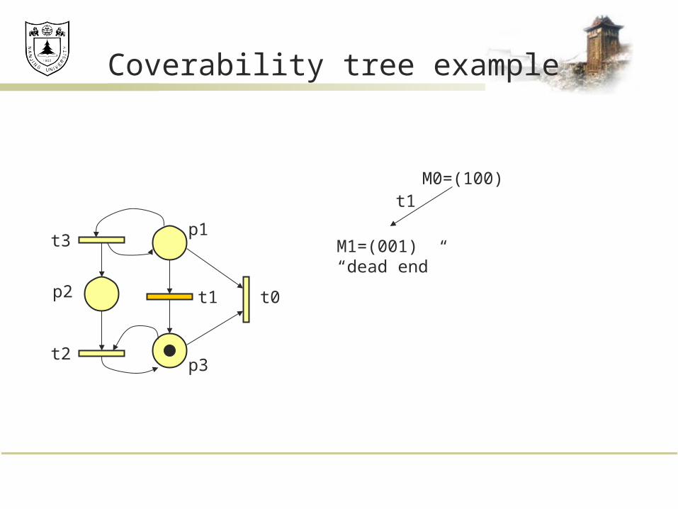
Analysis methods (1)
Coverability tree tree representation of all possible markings
root = M0
nodes = markings reachable from M0
arcs = transition firings if net is unbounded, then tree is kept finite by introducing
the symbol Properties
a PN is bounded iff doesn’t appear in any node a PN is safe iff only 0’s and 1’s appear in nodes a transition is dead iff it doesn’t appear in any arc if M is reachable form M0, then exists a node M’ that covers M

Coverability tree example
t3
p2
t2
p1
t1
p3
t0
M0=(100)
Coverability tree example
t3
p2
t2
p1
t1
p3
t0
M0=(100)
M1=(001)“dead end”
t1

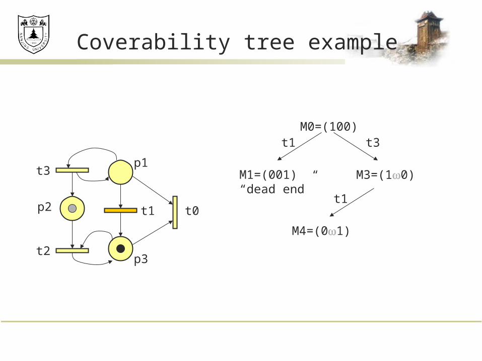
Coverability tree example
t3
p2
t2
p1
t1
p3
t0
M0=(100)
M1=(001)“dead end”
t1 t3
M3=(10)
Coverability tree example
t3
p2
t2
p1
t1
p3
t0
M0=(100)
M1=(001)“dead end”
t1 t3
M3=(10)
t1
M4=(01)
Coverability tree example
t3
p2
t2
p1
t1
p3
t0
M0=(100)
M1=(001)“dead end”
t1 t3
M3=(10)
t1
M4=(01)
t3
M3=(10) “old”

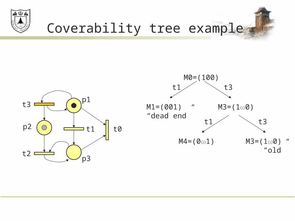
Coverability tree example
t3
p2
t2
p1
t1
p3
t0
M0=(100)
M1=(001)“dead end”
t1 t3
M3=(10)
t1
M4=(01)
t3
M6=(10) “old”
t2
M5=(01) “old”
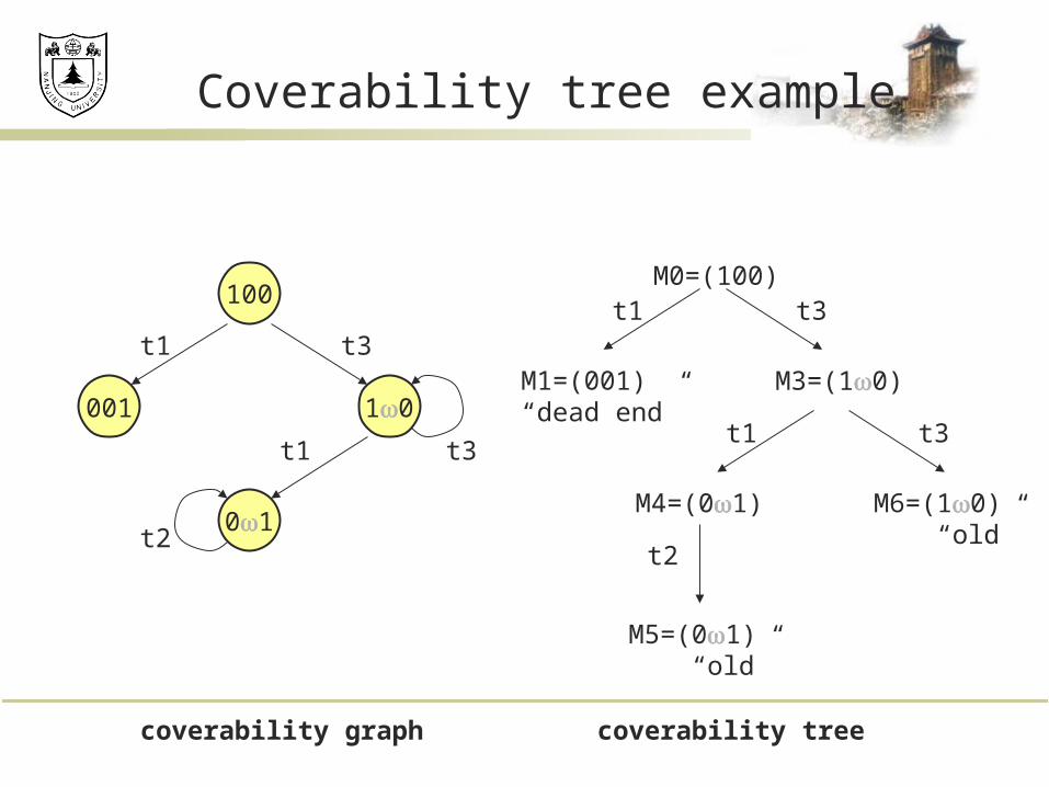
Coverability tree example
100M0=(100)
M1=(001)“dead end”
t1 t3
M3=(10)
t1
M4=(01)
t3
M6=(10) “old”
t2
M5=(01) “old”
t1 t3
t1
10001
01
t3
t2
coverability graph coverability tree
Reduction Rules
Analysis of Petri nets tedious, especially for large, com-plex nets
Often, the complexity for analysis increases exponentially with the size of the Petri net
Solution: Simplify the net while retaining the properties to analyze.
In our case, the properties in question are Liveness Safeness Boundedness
6 of the simplest reduction rules are shown in the sequel
60

Reduction Rules
61
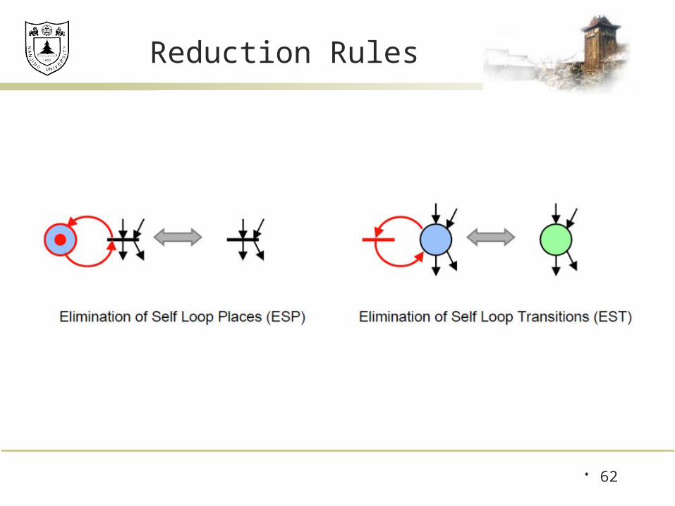
Reduction Rules
62

Common Extensions
Colored Petri nets: Tokens carry values (colors)
Any Petri net with finite number of colors can be
transformed into a regular Petri net. Continuous Petri nets: The number of tokens can be real.-
Cannot be transformed to a regular Petri net Inhibitor Arcs: Enable a transition if a place contains no to-
kens. Cannot be transformed to a regular Petri net
63

Time Extension
The previous examples model the sequences of events that can take place in the system; for example, they tell us that "the resource must be occupied before being re-leased", or that "a new low-priority request can be is-sued only after the resource is released", but it does not say anything about time distances e.g. how soon is the resource granted after a low-priority
request? how long can a process keep the resource occu-pied? how often is a new request issued?
to be able to model these properties, we need to introduce a quantitative notion of time into the formalism
64

Petri Net with Time
Time Petri nets are classical Petri Nets where to each transition t a time interval [a; b] is associated. The times a and b are relative to the moment at which t was last enabled. Assuming that t was en-abled at time c, then t may fire only during the in-terval [c + a; c + b] and must fire at the time c + b at the latest, unless it is disabled before by the firing of another transition. Firing a transition takes no time.
65
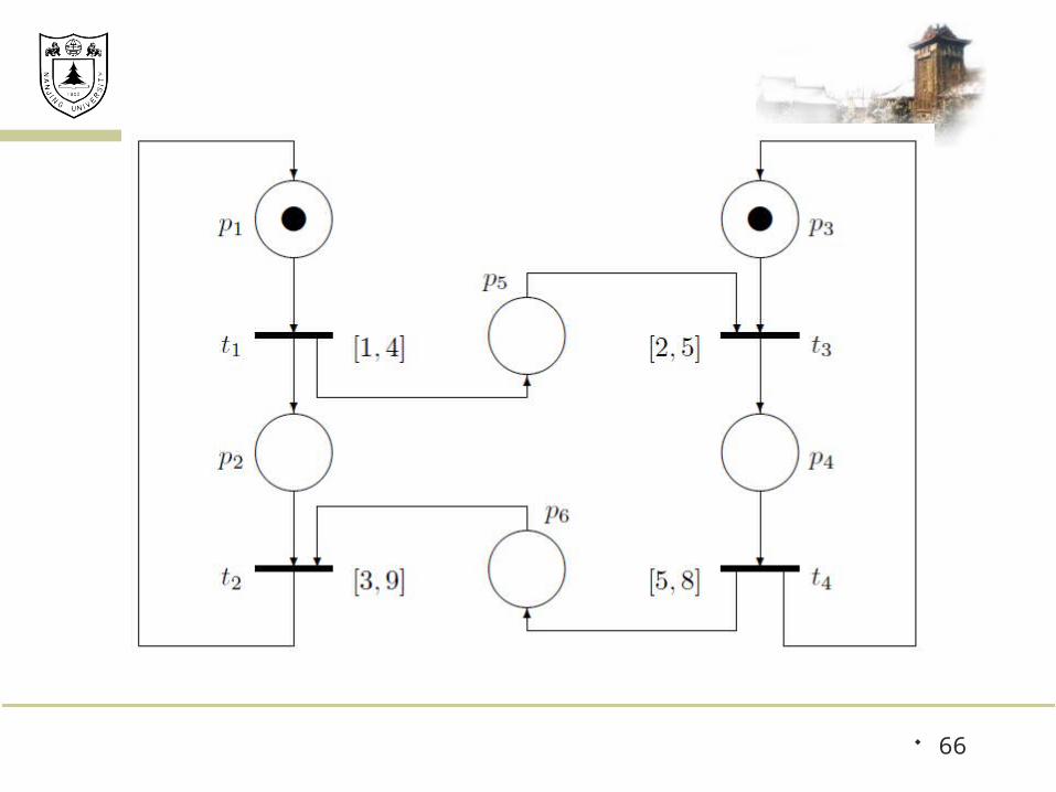
66

The philosophy of this kind of time dependent Petri net is: when a transition becomes enabled it may not fire at once (in general) but during a certain time in-terval and at the end of the interval there is a force to fire. If the upper bound of the interval is at infinity, then the second characteristic, the obligation to fire, is lost. That is why we consider only time intervals whose upper bounds are finite numbers.
67
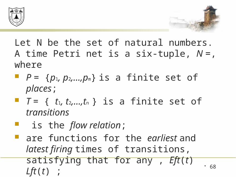
Let N be the set of natural numbers. A time Petri net is a six-tuple, N =, where P = {p1, p2,…,pm} is a finite set of places; T = { t1, t2,…,tn } is a finite set of transitions is the flow relation; are functions for the earliest and latest firing times
of transitions, satisfying that for any , Eft(t) Lft(t) ; P is the initial marking of the net.
68

Let the domain of time values T be the set of nonnega-tive real numbers.
A state of a time Petri net N =, is a pair where is a marking of N, and c : enabled() T is called the clock function. The initial state of N is where (t) = 0 for any t enabled().
69

A transition t may fire from state after delay T if and only if the following conditions hold: t enabled(), (-t) t = , Eft(t) c(t) +, and t’ enabled(): c(t’) +Lft(t’).
70
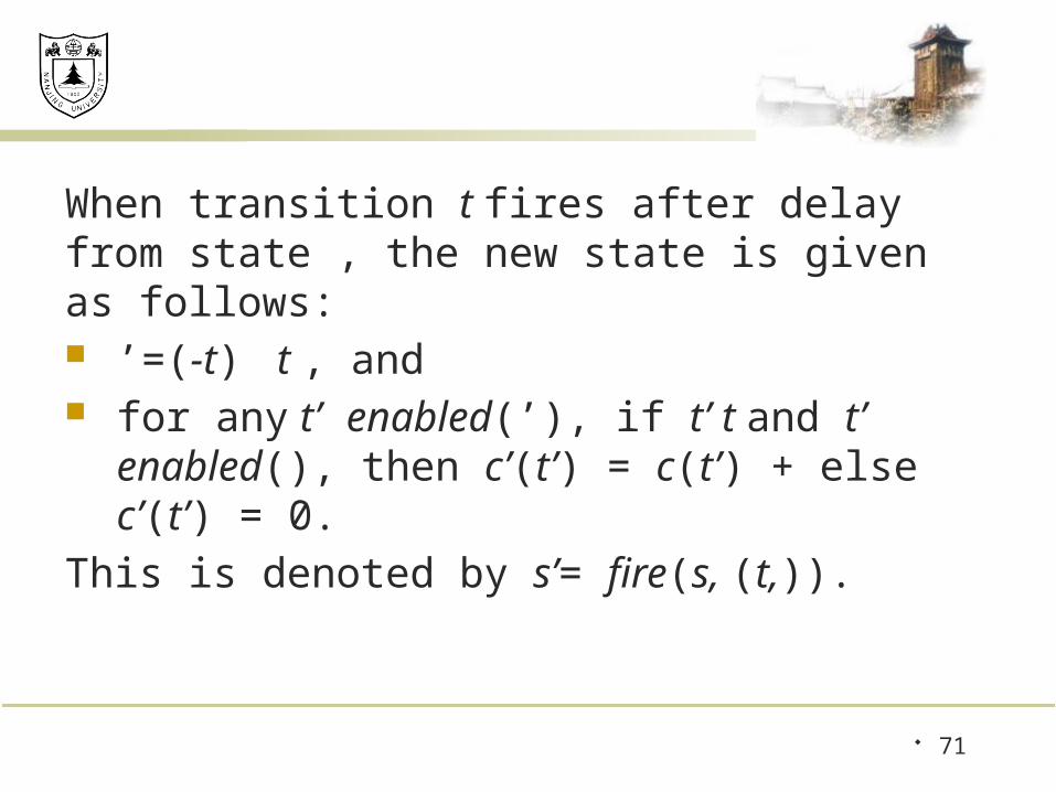
When transition t fires after delay from state , the new state is given as follows: ’=(-t) t , and for any t’ enabled(’), if t’ t and t’ enabled(), then
c’(t’) = c(t’) + else c’(t’) = 0.
This is denoted by s’= fire(s, (t,)).
71

A run …
of a time Petri net is a finite or infinite sequence of states, transitions, and delays such that is the initial state, and for every i 1, is obtained from by firing a transition after delay which satisfies that =fire(,(, )).
72
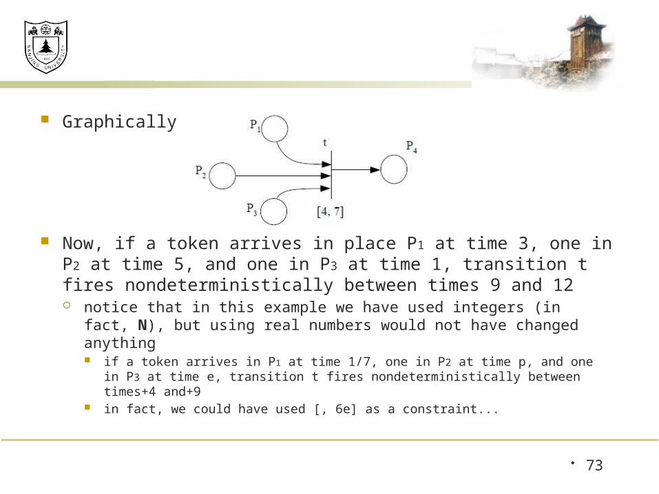
Graphically
Now, if a token arrives in place P1 at time 3, one in P2 at time 5, and one in P3 at time 1, transition t fires nondeterministically be-tween times 9 and 12 notice that in this example we have used integers (in fact, N), but using
real numbers would not have changed anything if a token arrives in P1 at time 1/7, one in P2 at time p, and one in P3 at time e,
transition t fires nondeterministically between times+4 and+9 in fact, we could have used [, 6e] as a constraint...
73

Simultaneous Firing
With untimed PNs, the notion of simultaneous firing (for non-con-flicting transitions) was irrelevant –for example, consider the following fragment of PN:
after r fires, producing a marking that we call M, it does not matter whether it is u or v that fires first from M: from the point of view of the un-timed model, the firing sequence u, v does not mean that u fires at time t, and v first at a later time t' > t, since there is no notion of time! •untimed PNs represent sequences of firings, but these are logical sequences, not
temporal ones
74

However, in the timed model simultaneity can occur, in the sense that two firings are associated with the same instant –let us now consider the previous fragment of PN, and add time:
now, if r fires at time 10, both u and v can fire at time 14, so both fir-ing sequences <r, 10>, <u, 14>, <v, 14> and<r, 10>, <v, 14>, <u, 14> are admissible notice that the firings of u and v are associated with the same time instant, so
they are in effect simultaneous
75
In the previous example, there was no logical ordering between u and v: they could occur at the same time, but neither had to fire before the other this was represented by the fact that both the <r, 10>, <u,
14>, <v,14> and the <r, 10>, <v, 14>, <u, 14> sequences are admissible
However, there could be a different form of simul-taneity, one which however entails logical ordering
76

Let us consider the following fragment of TPN:
in this case, when r fires, s must fire at the same time (that is, the firing of r and the one of s must be associated with the same temporal instant) that is, sequences are of the form <r, T>, <s, T>
however, there is a logical precedence between r and s, in the sense that, in all firing sequences, the firing of r must precede the one of s i.e. sequence <s, T> <r, T> is not admissible
77
Transitions in which the lower bound is 0 (such as transitions above) are called zero-time transitions, since they can occur at the same time in which they are enabled, without delay zero-time transitions, if not treated carefully, can give
rise to the so-called Zeno-behavior
78

a Zeno behavior is one in which time does not ad-vance
Let us consider the following fragment of TPN:
the following sequence of firings is admissible (for any T in which place p contains a token): <s, T>, <v, T>, <r, T>, <s, T>, <v, T>, <r, T>, <s, T>, ... in such a sequence time is not advancing (even if the sequence
grows!), which is physically impossible
79

One might argue that zero-time transitions in the real world cannot occur, so we should avoid them entirely however, even if they are not physically feasible, from
the point of view of modeling they are often useful, for example to model cases in which the difference in time between two transitions is negligible with respect to the main dynamics of the system
80

Example: Kernel Railorad Crossing
Kernel = simplified: there is only one train dm and dM are, respectively, the minimum and maximum time to go from the begin-
ning of section R to the beginning of section I hm and hM are, respectively, the minimum and maximum time to go through I the gate can be open or closed but also moving up and down the moving of the gate takes time units and cannot be interrupted
as mentioned, this is the simplified version of the problem; the Generalized Railroad Crossing (GRC) has many trains and tracks, the movement of the gate can be interrupted, etc.
81

Does this model guarantee that the gate will always be closed if a train is in section I?
82
Petri Net World http://www.informatik.uni-hamburg.de/TGI/PetriNets/
83

TINA Demo
84


![Discrete timed Petri nets - Pure - Aanmelden · colored Petri nets. We also do not consider continuous Petri nets (cf [31]) because the underlying untimed net is not a classical Petri](https://static.documents.pub/doc/80x56/601b8a6f707ca30c043d37a8/discrete-timed-petri-nets-pure-aanmelden-colored-petri-nets-we-also-do-not.jpg)


