econstor www.econstor.eu Der Open-Access-Publikationsserver der ZBW – Leibniz-Informationszentrum Wirtschaft The Open Access Publication Server of the ZBW – Leibniz Information Centre for Economics Standard-Nutzungsbedingungen: Die Dokumente auf EconStor dürfen zu eigenen wissenschaftlichen Zwecken und zum Privatgebrauch gespeichert und kopiert werden. Sie dürfen die Dokumente nicht für öffentliche oder kommerzielle Zwecke vervielfältigen, öffentlich ausstellen, öffentlich zugänglich machen, vertreiben oder anderweitig nutzen. Sofern die Verfasser die Dokumente unter Open-Content-Lizenzen (insbesondere CC-Lizenzen) zur Verfügung gestellt haben sollten, gelten abweichend von diesen Nutzungsbedingungen die in der dort genannten Lizenz gewährten Nutzungsrechte. Terms of use: Documents in EconStor may be saved and copied for your personal and scholarly purposes. You are not to copy documents for public or commercial purposes, to exhibit the documents publicly, to make them publicly available on the internet, or to distribute or otherwise use the documents in public. If the documents have been made available under an Open Content Licence (especially Creative Commons Licences), you may exercise further usage rights as specified in the indicated licence. zbw Leibniz-Informationszentrum Wirtschaft Leibniz Information Centre for Economics Karlan, Dean; Linden, Leigh L. Working Paper Loose Knots: Strong versus Weak Commitments to Save for Education in Uganda IZA Discussion Paper, No. 7901 Provided in Cooperation with: Institute for the Study of Labor (IZA) Suggested Citation: Karlan, Dean; Linden, Leigh L. (2014) : Loose Knots: Strong versus Weak Commitments to Save for Education in Uganda, IZA Discussion Paper, No. 7901 This Version is available at: http://hdl.handle.net/10419/93261
Transcript
econstor www.econstor.eu
Der Open-Access-Publikationsserver der ZBW – Leibniz-Informationszentrum WirtschaftThe Open Access Publication Server of the ZBW – Leibniz Information Centre for Economics
Standard-Nutzungsbedingungen:
Die Dokumente auf EconStor dürfen zu eigenen wissenschaftlichenZwecken und zum Privatgebrauch gespeichert und kopiert werden.
Sie dürfen die Dokumente nicht für öffentliche oder kommerzielleZwecke vervielfältigen, öffentlich ausstellen, öffentlich zugänglichmachen, vertreiben oder anderweitig nutzen.
Sofern die Verfasser die Dokumente unter Open-Content-Lizenzen(insbesondere CC-Lizenzen) zur Verfügung gestellt haben sollten,gelten abweichend von diesen Nutzungsbedingungen die in der dortgenannten Lizenz gewährten Nutzungsrechte.
Terms of use:
Documents in EconStor may be saved and copied for yourpersonal and scholarly purposes.
You are not to copy documents for public or commercialpurposes, to exhibit the documents publicly, to make thempublicly available on the internet, or to distribute or otherwiseuse the documents in public.
If the documents have been made available under an OpenContent Licence (especially Creative Commons Licences), youmay exercise further usage rights as specified in the indicatedlicence.
zbw Leibniz-Informationszentrum WirtschaftLeibniz Information Centre for Economics
Karlan, Dean; Linden, Leigh L.
Working Paper
Loose Knots: Strong versus Weak Commitments toSave for Education in Uganda
IZA Discussion Paper, No. 7901
Provided in Cooperation with:Institute for the Study of Labor (IZA)
Suggested Citation: Karlan, Dean; Linden, Leigh L. (2014) : Loose Knots: Strong versus WeakCommitments to Save for Education in Uganda, IZA Discussion Paper, No. 7901
This Version is available at:http://hdl.handle.net/10419/93261
DI
SC
US
SI
ON
P
AP
ER
S
ER
IE
S
Forschungsinstitut zur Zukunft der ArbeitInstitute for the Study of Labor
Loose Knots: Strong versus Weak Commitments toSave for Education in Uganda
IZA DP No. 7901
January 2014
Dean KarlanLeigh L. Linden
Loose Knots:
Strong versus Weak Commitments to Save for Education in Uganda
Dean Karlan Yale University,
IPA, M.I.T. J-PAL, NBER, and Center for Global Development
Any opinions expressed here are those of the author(s) and not those of IZA. Research published in this series may include views on policy, but the institute itself takes no institutional policy positions. The IZA research network is committed to the IZA Guiding Principles of Research Integrity. The Institute for the Study of Labor (IZA) in Bonn is a local and virtual international research center and a place of communication between science, politics and business. IZA is an independent nonprofit organization supported by Deutsche Post Foundation. The center is associated with the University of Bonn and offers a stimulating research environment through its international network, workshops and conferences, data service, project support, research visits and doctoral program. IZA engages in (i) original and internationally competitive research in all fields of labor economics, (ii) development of policy concepts, and (iii) dissemination of research results and concepts to the interested public. IZA Discussion Papers often represent preliminary work and are circulated to encourage discussion. Citation of such a paper should account for its provisional character. A revised version may be available directly from the author.
Loose Knots: Strong versus Weak Commitments to Save for Education in Uganda*
Commitment devices offer an opportunity to restrict future choices. However, if severe restrictions deter participation, weaker restrictions may be a more effective means of changing behavior. We test this using a school-based commitment savings device for educational expenses in Uganda. We compare an account fully-committed to educational expenses to an account in which savings are available for cash withdrawal but intended for educational expenses. The weaker commitment generates increased savings in the program accounts and when combined with a parent outreach program, higher expenditures on educational supplies. It also increases scores on an exam covering language and math skills by 0.14 standard deviations. We find no effect for the fully-committed account, and we find no effect for either account on attendance, enrollment, or non-cognitive skills. JEL Classification: D12, D91, I21, O12 Keywords: commitment savings, micro-savings, educational resources, school participation Corresponding author: Leigh L. Linden Department of Economics The University of Texas at Austin 2225 Speedway, C3100 Austin, Texas 78712 USA E-mail: [email protected]
* We are grateful for the assistance of a number of individuals and organizations without whom this project could not have been successfully completed. Carl Brinton, Sarah Kabay, Sana Khan, Selvan Kumar, Doug Parkerson, Pia Raffler, Elana Safran and Glynis Startz from Innovations for Poverty Action all provided valuable assistance with the research or project management. We gratefully acknowledge the financial support of the Yale Savings and Payments Research Fund at Innovations for Poverty Action, sponsored by a grant from the Bill & Melinda Gates Foundation. The United States Agency for International Development (Development Innovations Venture Award AID-OAA-G-12-00008) generously provided additional funding for the project. All opinions are those of the authors, and not necessarily that of any of the funders or collaborating institutions.
“Make it easy” – Richard Thaler, co-author of Nudge: Improving Decisions about Health, Wealth, and Happiness (Clement 2013)
Section I. Introduction
We test whether a strong versus weak savings commitment device helps children and their families save more, spend more on educational expenses, and achieve higher test scores. We are motivated by three issues. First, we want to examine the net tradeoff between higher participation but lower compliance from weak commitment devices and lower participation but higher compliance from strong commitment devices. This thus becomes a test between a stricter commitment device and a weaker “make it easy” nudge of individuals towards a specific behavior (Thaler and Sunstein 2009). Second, we test for changes in expenditures, to answer a question that often lingers around interventions that aim to increase savings (Karlan, Ratan, and Zinman 2013): did the increased savings in one vehicle change actual expenditures, or simply come from a reshuffling of one’s balance sheet across different products? Finally, we test whether an intervention which leads to higher investment by households in school supplies then improves educational outcomes for children. This has implications for the production function of primary school education, and potential methods for relaxing financing constraints that hinder educational progress for children.
Commitment devices offer individuals an opportunity to restrict future choices. Self-aware individuals may prefer such restrictions in order to resist future temptations, or to deflect future claims on assets from family or extended social networks. Indeed, prior research has found demand for savings accounts that restrict access to one’s money in order to help with self-control issues (Ashraf, Karlan, and Yin 2006).
However, the specifics of what one means by “commitment” on a commitment savings account can vary in critical ways, and accordingly have large differential impacts on whether an account is opened, how much one deposits, when one withdraws, and perhaps most importantly, how ultimate consumption and investment choices differ. We focus here on one key dimension: whether the funds deposited are locked in for a specific “good” expenditure, or if individuals have freedom to spend withdrawals as they wish, but the “good” item is made easily available.1
The tradeoff is clear: a strong commitment device may be more effective in enforcing the behavior of the future self, but the current self may be less likely to participate in the contract at all. An individual may want to commit in some, but not all, future states of the world, since emergencies do happen. The challenge is finding a contract where a third party has the right level
1 Clearly in a perfect market, specifically one with zero transaction costs, this would make no difference: any items purchased with the locked-in commitment account could simply be sold in exchange for the most desirable item for the same value. In our market, supplies and services associated with primary education in Uganda, there are significant enough transaction costs to make such an exchange quite costly, and thus the original expenditure sticky.
2
of discretion on whether to enforce. If an individual cannot trust any third parties with that discretion, a self-enforcing commitment contract may work instead. In such a contract, the increased price of vice is derived from psychic costs, i.e., disappointment with oneself and one’s lack of adherence to a plan. This is akin to a model put forward by Benabou and Tirole (2004)(2004) on how personal rules can shift later behavior, and also could be construed as a test of whether “mental accounting” can be an policy instrument that induces behavior change (Shefrin and Thaler 1992).
However, a shift in savings behavior may not matter, if there are offsetting behaviors. For example, more money saved in a commitment account may come at the expense of lower savings elsewhere, or worse, higher borrowing at higher interest rates. By examining how actual expenditures change, rather than merely observing whether savings increases, we are able to make stronger statements about welfare outcomes, similar to Ashraf et al (2010) with respect to household durable goods purchases and Dupas and Robinson (2013) with respect to health investments.
The savings program helps families save for school related expenses and generates random variation in the level of school supplies across students. This thus allows us to better understand the education production process (Kremer and Holla 2009). In particular, we contribute to two areas of the literature. First, we build on a growing body of evidence demonstrating the effects of basic school supplies – notebooks, uniforms, workbooks, etc. – on student performance (Das et al. 2013; Hidalgo et al. 2013) and parental involvement (Avvisati et al. 2013). Second, the results build on existing evidence of the importance of savings constraints for educational expenses (Barrera-Osorio et al. 2011).2
Our setup is as follows: working with a local nonprofit organization Private Education Development Network (PEDN) in the Busoga sub-region of the Eastern region of Uganda, and Innovations for Poverty Action (IPA), we randomly assigned 136 primary schools to one of three groups: a strong commitment savings account, a weak commitment savings account, or control. For both treatments, students could deposit cash into an account. Although the accounts were framed as their accounts, we cannot rule out that some of the funds were parent’s funds..3 We developed a brief teacher training component, and also coordinated the transfer of money from a savings box held at the school to a local bank for safekeeping. One year into the implementation, we implemented one sub-treatment in half of the treatment schools, a parental involvement workshop.
2 It is interesting to note that, while we find that relaxing savings constraints improves educational outcomes, we find improvements in academic performance rather than participation. This contradicts the results of Barrera-Osorio et al. (2011) which finds that distributing funds at the time that families have to pay enrollment expenses improves enrollment rates. The difference may, in part, be due to the fact that unlike Uganda, Colombian schools still charged official fees for enrollment. 3 As we show below, both the children and other family members contribute to the accounts, raising the possibility that multiple household mechanisms are involved.
3
The first stage is critical and revealing: students deposit significantly more money into the soft commitment savings account than the hard commitment savings account. And, for those with the parental outreach sub-treatment, the additional money deposited into the account leads to higher investment in school supplies, which then in turn leads to higher test scores. We find a 0.13 standard deviation (se=0.04) improvement in overall scores; this includes effects on each of the covered subjects: grammar (0.12 standard deviations, se=0.04), reading (0.13 standard deviations, se=0.05), and math (0.08 standard deviation, se=0.04). The implication for the school production function is simple: for a student to learn basic skills, having a pen, paper and workbook matters. Furthermore, the treatment effect on educational outcomes is sizable, as large as many direct educational interventions, and consistent with other estimates of the effects of such supplies (Das et al. 2013) We find no effect on student participation (either attendance or enrollment) or on a set of non-cognitive outcomes.
The remainder of the paper proceeds as follows: We provide an overview of the Ugandan education system and the individual treatments in Section II. Section III contains the research design and a description of the data. We assess the internal validity in Section IV and present the main results in Section V. Finally, we conclude in Section VI.
Section II. Background
A. Ugandan Primary Education System
Uganda abolished most primary school fees in 1997.4 In the same year, the gross primary enrollment rate5 ballooned from 87 percent in the early 1990s, to 123 percent in 1997. Between 1997 and 1996, 2.3 million children enrolled in primary school, increasing total enrollment to 5.7 million (“Uganda Hits Universal Primary Education Target” 2000).
Unfortunately, while most children now enroll in primary school, the majority of them fail to graduate. In 2008, for example, the gross enrollment rate6 in lower secondary was 33 percent–11 percentage points below the average for Sub-Saharan Africa (UNESCO 2013). The transition from primary to secondary is a challenge, as in many countries. However, the majority of Ugandan students simply fail to complete primary school. As of 2010, only 32 percent of students entering primary school completed the seventh grade (“Opportunities Lost: The Impact of Grade Repetition and Early School Leaving” 2012).
4 Initially, up to four children per family could attend school without paying tuition fees. However, previously the government abolished tuition fees for all children (Murphy, Bertoncino, and Wang 2002). 5 The net primary school enrollment ratio is the ratio of the number of enrolled primary school children, regardless of age, to the total number of primary school-aged children in the population. 6 The gross enrollment rate for lower secondary school is the ratio of the number of children enrolled in lower secondary school regardless of age relative to the total number of children in the population who are of age to attend secondary school.
4
While the poor quality of primary education is a likely factor (Piper 2010),7 students still face financial barriers. Students no longer pay enrollment fees, but they face other expenses. Many schools require uniforms, and families are responsible for providing food and school supplies, such as paper, writing instruments, and workbooks. With the approval of the parent-teacher association and school management committee, schools can also charge fees for ancillary services such as supplementary lessons, practice exams and feeding programs. Official policy prohibits preventing a child from enrolling due to an inability to pay, but the majority of dropouts cite financial concerns. In the baseline survey described below, families paid an average of 5,790 UGX (2.30 USD) to send a child to school for a year, 0.5 percent of Uganda’s per capita income in 2010 (UN data 2013).
Confusion and suspicion create additional complications. As we discovered through qualitative interviews and feedback from parents, politicians try to drum up support by claiming school fees are illegal. The terms “universal” and “free” education are sometimes used interchangeably. Many parents do not understand the official financing rules. Some believe that the government should provide for all school related expenses. Finally, rumors of corruption can make even knowledgeable parents reluctant to pay.
B. Description of the Intervention
To facilitate families’ and children’s saving for school, we evaluated four variations of a school-based savings program. The intervention had two primary objectives. First, it sought to facilitate and encourage the practice of children saving for education, and through saving, improve overall academic performance and support students’ continued enrollment. The program targeted students in grades 5, 6, and 7, the last three years of primary school, in order to target students at high risk for dropping out of school.8
We developed and implemented the programs in partnership with the Private Education Development Network (PEDN). PEDN is a Ugandan non-profit organization focusing on youth financial and entrepreneurial education. PEDN comprises five full and part time employees, often supplemented by project specific staff that PEDN hires as needed. For the savings programs, IPA worked with PEDN to hire a local implementation team of about 10 people.9
Each of the four treatment variations included the same core components: a savings account administered through the school, and a program to support and encourage use of the accounts. During an introductory meeting, the implementation team described the program to a joint
7 The dramatic increases in enrollment have strained existing resources. In the average school in 2005, three children had to share the same textbook and 94 children crammed into a single classroom (Independent Evaluation Group (IEG) 2007). 8 Uganda follows a 7+2+2 grade structure. Students attend primary school for seven years followed by two years each of lower and then upper secondary school. 9 This includes only those individuals hired to implement the described programs. It does not include the research staff who conducted the surveys and monitoring visits described below.
5
meeting of the Parent Teacher Associate, the School Management Committee, and other interested parents. If they all voted to participate, we provided each school with metal lock boxes. A designated teacher assisted by student-elected10 representatives from each class then managed the program. The implementation team conducted weekly visits to each school to encourage saving and to assist with accounting procedures. Interested students received a passbook in which their individual savings were recorded, and the designated teacher and the implementation team maintained an official register. Depending on a school’s preference, students then deposited money into the lockboxes on a daily or weekly basis.
To provide security and transparency, two padlocks secured each box. Parents elected a representative to keep the key to one lock, while the bank held the other. At the end of each trimester,11 the two key holders opened the box. The bank representative provided a deposit slip and deposited the funds into the school’s account.12 The accounts did not earn interest. Inflation varied but averaged around 10% in this time period, thus the accounts had a negative real interest rate. After the break between trimesters, the implementation team and bank representatives returned to the school for the payout of the funds. Two representatives signed a withdrawal slip to confirm the withdrawal. The designated teacher, student representatives and our team then distributed the money according to the savings register. At the same time, the implementation team organized a small market at each school where students could purchase school supplies or school services such as practice exams or tutoring sessions.13
On top of the core components above, there were four treatment variations, a 2x2 design: “cash” or “voucher” for the withdrawals, and “Parent Outreach” or “No Parent Outreach”. For the cash treatment arm, students received, in cash, their savings from one trimester at the beginning of the next trimester. They could then spend the funds at their discretion—at the markets provided on the disbursement day (thus “making it easy” to spend on school supplies) or elsewhere. The voucher treatment arm, on the other hand, employed a stronger commitment — students had to buy educational products or services at the market, on the disbursement day. In both variants, children could also re-deposit their savings for the next trimester.
The Parent Outreach component provided a means of addressing misconceptions about school fees and Universal Primary Education Policy. The implementation team hosted a meeting for sixth and seventh grade parents. The meetings began by identifying the various stakeholders in
10 The Ugandan educational system classifies children enrolled in primary school as “pupils” and those in secondary school as “students”. In this article, we refer to all enrolled children as students. 11 The academic year starts in February and follows a trimester system. Schools run for 12 weeks at a time. Students receive a three week break after the first and second terms, and schools are closed in December, January and February. 12 Working with the bank, FINCA Uganda, we designed an account for the intervention modeled on a traditional group savings account. We also provided the minimum 5,000 UGX deposit and worked with the school’s elected signatories to obtain the documentation required to open the accounts. 13 Students were allowed to rollover vouchers to future terms, and upon completion of the final year (P7), were allowed to withdraw any remaining balance in cash.
6
primary education, their roles and responsibilities. PEDN then discussed the various ways in which parents could support their children’s education. In particular, PEDN explained that in addition to providing a student learning experience, the savings program provided an opportunity for the household. It could be a tool to help families finance their children’s education. A snack and soda were provided to encourage attendance.
Section III. Design of the Evaluation
A. Research Design
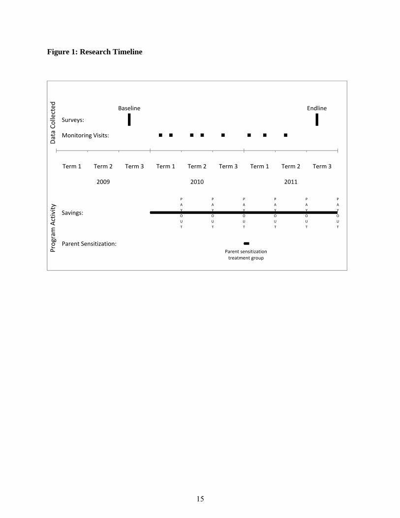
Figure 1 depicts the timeline and steps in the randomized trial and data collection. We selected 136 primary schools from the Jinja, Iganga, Mayuge, and Luuka districts of the Busoga Region because they predominantly comprised poor rural and peri-urban schools. We then administered a baseline survey and test during the final trimester of 2009. Finally, we randomly assigned schools to receive either the cash treatment, voucher treatment, or no treatment, stratifying by the total normalized score on the baseline exam and by geographic regions call sub-counties.14 Each treatment group comprised 39 schools, and the remaining 58 schools became the control group.
Following the first randomization, school outreach began. It took two trimesters to recruit the majority of schools, but by the beginning of the third trimester of 2010, 95 percent of the treatment schools had agreed to participate.15 In total, 77 schools joined and one school refused to participate. The school that refused to participate did, however, permit data collection. In what follows, we classify the school as if it had accepted the program.
In 2011, we conducted a second randomization for the parent sensitization program. To isolate the effect of the program while still treating all of the schools, we assigned schools either to the Parent Outreach group who received the intervention in the first trimester of 2011 or to the No Parent Outreach group who received the intervention too late to affect student behavior – immediately before the endline survey in second trimester. Half of the schools in each treatment were assigned to each group. We stratified assignment by the schools’ initial treatment group and sub-county, and checked for balance using the demeaned savings rates from 2010.
Finally, we conducted the endline survey and exam during the beginning of the third trimester of 2011.16
14 In 2010, Uganda included four major jurisdictions called “regions.” Spread across the four regions, were 111 “districts.” Each district was divided into urban areas known as “municipalities” or rural areas called “counties.” Counties were further sub-divided into sub-counties. Depending on the population, a district could have as few as three or as many as thirty or more sub-counties. 15 When they were not canceled, meetings had to be held with school administrators, the school management committee, and the parent-teacher association for each school. Many were initially reluctant to hold additional meetings. 16 In 2012, we conducted a second, smaller experiment in which we randomly assigned a fraction of the original control group to receive the cash with sensitization program. We also collected the classroom-level data described below. However, the remaining control group proved too small. The point estimates are consistent with those
7
B. Description of the Datasets
The study utilizes two samples of students, as well as data at both the classroom and student level. First, we conduct classroom level surveys that include all students present in class at baseline and then all students present in class at endline. Second, we created a representative, longitudinal sample of students identified prior to the randomization. The first sample provides information on all students attending school. However, if the intervention had affected attendance or enrollment, it would have been subject to selection biases, both on entry and exit. The second sample provides information on a smaller subset of students that were tracked regardless of whether or not they continued to be enrolled in the original schools.
The classroom-level data included all classes in grades five, six, and seven. Enumerators counted the number of children present, enrolled and possessing notebooks, math set, uniform, or shoes.17,18 We conducted these monitoring visits prior to the randomization as part of the baseline and at least once a trimester after the randomization.
The student-level data was created by selecting 4,716 students who then completed a baseline survey and aptitude test prior to the randomization. To identify the students for the longitudinal sample, we compiled a list of all students of the correct ages and grades who were on the teachers’ rosters in September of 2009.19 Teachers then classified each student using a five-point scale to rate frequency of attendance. In particular, this allowed us to identify students on the rosters who did not attend school. From the set of attending children, we randomly selected 35 students from each school in grades four and five, except for two schools in which we included all students because fewer than 35 students had enrolled.
The baseline survey completed by the students in the longitudinal sample was a 40 minute survey that included questions about their education history, experiences with saving, time preferences, and demographic information. Students also completed an hour-long, 35-question exam covering math, grammar, and reading comprehension. Students in each grade took separate exams based on the national curriculum for their grade.20
Students completed an endline survey about two years after the base line survey. The 40 minute survey included questions about saving behavior, possession of resources like those in the class-level survey, such as uniforms, books, math sets, and shoes. It also included a 60 minute exam in
presented here, but the standard errors are too large to provide meaningful information. These results are available upon request. 17 The enumerator only counted a student as having each item if the enumerator could see it. 18 Notebooks cost approximately 200 UGX (0.08 $USD) each. In Uganda, they are usually called “exercise books.” A math set costs approximately 1,000 UGX (0.40 $USD) and includes such tools as a ruler, protractor and compass. Uniform and shoes each cost about 6,000 UGX. (2.39 $USD) They are a traditional school requirement. 19 For a small number of classes, rosters were unavailable. We had to create a list of students based on the students present in class and information provided by the teacher. 20 For both the baseline and endline exams, all scores are normalized within grade and subject relative to the contemporaneous control distribution.
8
the same three subjects as the baseline exam. The grade level of the endline exam was based on the students’ grade at baseline. We tracked students regardless of their enrollment status. We found 3,838 of the original respondents.
Finally, we verified the presence of each student in the longitudinal sample during each class-level monitoring visit. This provided an objective measure of students’ attendance rates as well as whether students were still enrolled in school in the appropriate grade.
C. Econometric Model
Since the random assignment should ensure the orthogonality of treatment assignment and other student characteristics, we estimate the effects of the treatments via Ordinary Least Squares using the following specification:
Yijk = α + τ’treatj + δ’Xik + εij. (1)
The variable Yijk is the dependent variable of interest. We perform estimates at the student and class level. The index i then represents either the student or class in school j and sub-county k. The vector treatj is a vector of indicator variables for each treatment, and Xik is a vector of control variables. For each estimate, we control for baseline test scores, sub-county fixed effects and the baseline value of the outcome if available. We cluster standard errors by the unit of randomization, the school.
Section IV. Internal Validity
In Table 1, we verify the effectiveness of the randomization in creating observably similar treatment and control groups on average. Each row presents estimates for the indicated baseline characteristic. Columns 1-3 provide the sample size for each variable,21 the pooled treatment mean and standard deviation, and the control mean and standard deviation. Column 4 provides the regression estimates of the difference between the combined treatment group and control group, while Columns 5-8 provide regression estimates of the difference between each treatment group and the control group. All differences are estimated using equation (1), controlling for the sub-counties in which the schools were stratified.
Overall, the differences are minimal, i.e., the assignment to each treatment is orthogonal to a series of baseline variables. Of the 70 estimates presented, only seven are statistically significant: one at the one-percent level, two at the five percent level, and four at the ten percent level. And the overall joint test of significance presented in the bottom row is not significant for any treatment group. Most importantly, the magnitudes of the estimated differences are also all relatively small.
21 Sample sizes vary because subjects refused to respond to some questions.
9
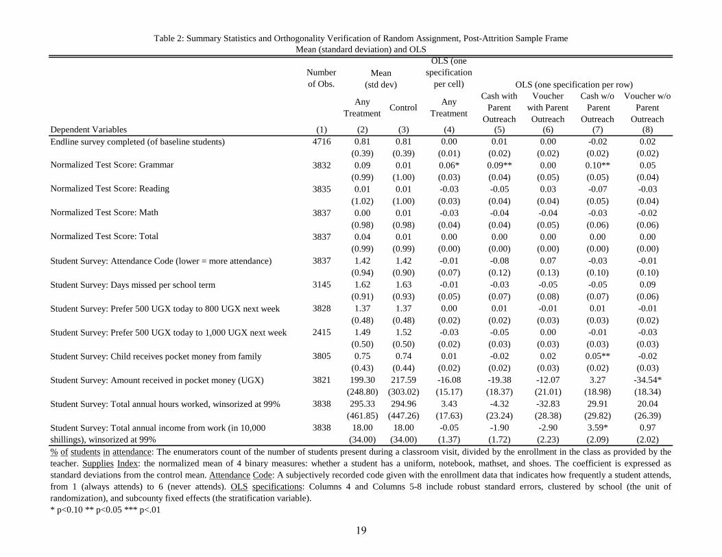
Even though the groups are comparable at baseline, differential attrition could result in differences in the analysis sample frame (i.e., those who complete the endline survey, or take the endline exams). Table 2 analyzes attrition. First, Row 1 presents the basic test for whether treatment led to differential attrition rates overall. Columns 2 and 3 show that we have identical survey completion rates in treatment and control (81 percent). Columns 5-8 show that we also find no differences across the four treatment groups.
However, even if overall survey completion rates are similar across treatment and control groups, the treatments may lead to different types of students completing the survey. To check for this, we replicate Table 1 analysis on various baseline measures. The table is organized similarly to Table 1 (except that the classroom variables are omitted, since there is no attrition at the classroom level). Overall, we find no evidence of compositional effects from differential attrition. Only six variables are statistically significant, and the only differences from Table 1 are the estimates for days missed per school term and amount of pocket money for the voucher treatment without parent sensitization. As with Table 1, the final row shows the aggregate tests, and we do not reject the null hypothesis of equality across treatment and control groups.
Section V. Results
First, we assess students’ savings behavior. In Table 3, we provide two measures of total savings over the two years of the program: the total per school and per student. Columns 1-4 provide the average for each research group. We draw three conclusions from these averages. First, the more restrictive savings vehicle, the voucher treatments, solicited significantly less savings than the less restrictive cash treatments. For both outcomes, the difference across the cash and voucher groups is statistically significant at the one percent level or less (Column 5). Second, we find no effect of the parent outreach on savings (Column 6). Finally, in results not provided in Table 3, we also find no effect of the parent outreach group within the cash treatment. This suggests that in the results below, the additional savings was driven primarily by the cash treatment and rather than increase savings further, the parent outreach direct these funds towards education.22
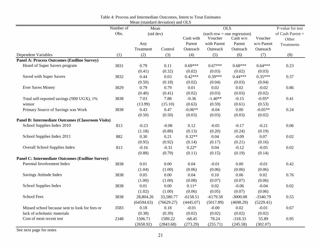
Table 4 examines the other process and intermediate outcomes. First, in Panel A, we examine process outcomes from the program itself, as reported by students in the endline survey. We find that 77 percent of treatment students and only 11 percent of control students were familiar with the Supersavers program. Similarly, 39 percent of treatment group students and only 4 percent of control group students reported saving with Supersavers. There was little difference in program awareness as well as self-reported participation on the extensive margin across treatment groups. This thus supports the argument that the difference in outcomes is not due to differential marketing or promotion of the program, or differential compliance to experimental protocols, but rather to the attractiveness of the cash versus voucher condition and the parent outreach. We do not find any increase in total self-reported savings (which in theory includes “savings held at 22 Interestingly, both parents and children contributed. According to the endline survey, 57 percent of children reported having earned the money that they deposited.
10
school”, i.e., savings held as part of this program), but we also consider these data noisy, as it is difficult to obtain accurate information on balances of informal savings, particularly from children. We thus put more weight on the administrative data (reported in Table 3) that shows participation in the program, and the changes in more easily observable and measured process and outcome changes, such as school supplies and test scores.
We then examine intermediate outcomes, i.e., the possession of school supplies (measured both during classroom visits as well as in the endline survey), parental involvement, savings attitudes, and payment of school fees. Analysis of these questions helps to understand the mechanism through which the program worked. We present the results for each, but only find an impact on the possession of school supplies, suggesting that the other mechanisms are not responsible for the observed impacts.
Table 4 Panel B presents the results on school supplies, as reported via classroom visits. The classroom visit school supplies index is normalized with respect to the control group mean and standard deviation, and takes the average of four proportions: proportion of students in the classroom possessing uniforms, notebooks, math sets, and shoes. In 2010, none of the treatment groups yields statistically significant increases relative to the control group. Relative to each other, the cash parent group is statistically different than the other treatment groups (Column 8), but this is partly the result of a decline in supplies experienced in two of the treatment groups. Relative to the control group, the cash with Parent Outreach treatment only improves by 0.11 standard deviations (se=0.11). Since the main difference between 2010 and 2011 is the addition of the Parent Outreach, the ineffectiveness of the cash treatments provides supporting evidence that the Parent Outreach is a necessary component.
For 2011, with an additional year of experience implementing the program and after the parent outreach had been fully launched, the Cash with Parent Outreach treatment arm performs considerably better than control, as well as the other three treatments (both when compared individually, as well as when the other treatments are pooled with control). Column 4 shows a 0.30 standard deviation improvement (se=0.14) compared just to control. This result is then reinforced by the endline survey, reported in Panel C: The school supplies index from the self-reported survey also shows in Column 4 a 0.22 standard deviation improvement (se=0.12) compared to control. We also find in Column 8, that the Cash with Parent Outreach is statistically different from the other treatments.23 We do not however observe any statistically significant shifts in school fees expenditures (albeit with large standard errors), self-reported absence because of failure to pay school fees, or amount paid for most recent tests.24
23 Appendix Tables 3d and 5 provide the details for each component of the supplies indexes in Panels B and C. The differences seem to be driven primarily by exercise books, although the individual components analysis is less robust statistically. 24 This pattern of results is consistent with students’ reports on the endline survey regarding the disposition of the saved funds. While the quality of the data are poor, we do observe that students in the cash treatment with the parent sensitization report spending 3.63 percent more of the saved funds on school related expenses than students in the
11
Table 4 Panel C also reports on data from the endline survey on parental involvement and savings attitudes. Although the school supplies and test score impacts are strongest on the Cash with Parent Outreach treatment cell, we do not observe a direct impact on an index of three questions25 regarding parental involvement in the child’s education (or the individual components, as reported in Appendix Table 3b). Furthermore, we do not observe changes in a savings attitudes index of seven questions.26 This may have implications for long-term change in saving behavior, if one posits that these attitudinal shifts are a necessary component for long-term behavior change, after the active involvement from the NGO and savings program. Alternatively, the measures may be flawed, or the attitudinal changes may be unnecessary; the learned pattern of savings may be possible to change without changing underlying savings attitudes.
Next we turn to test score results in Table 5. We put forward two basic mechanisms here: first, the savings account enables the purchasing of school supplies that are necessary for learning; second, the parental outreach leads the households and children to use the savings accounts to actually spend the saved money on school supplies. This is consistent with the results in Table 4 on the impact on school supplies. And likewise, this mechanism predicts that the Cash with Parent Outreach treatment group should generate the largest (or only) positive impacts. Column 4 indicates that Cash with Parent Outreach improves overall scores by 0.11 standard deviations (se=0.04). Looking at the components of the test, we find improvements in grammar (0.15 standard deviations, se=0.05) and reading (0.11 standard deviation, se=0.05), but no effect on math. Consistent with the hypothesized theory of change, none of the other three treatment groups generate statistically significant improvements compared to the control group, either overall or for any subject.
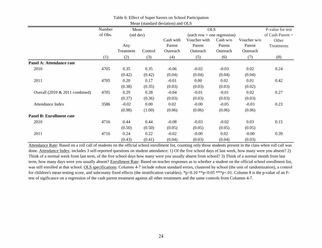
We also examine whether the improved test scores arises through increased attendance or enrollment, but find no evidence for either. Table 6 Panel A reports results on attendance, and Panel B reports results on enrollment. None of the treatments generate statistically significant improvements relative to the control group.
cash treatment without the sensitization. We observe no differences in the amount of the savings used to purchase food or clothing or given to other family members. The increase in school related expenditures primarily comes from “other” expenses. This difference, however, is likely too small to explain all of the observed increase in school supplies, suggesting that the parent sensitization functioned both to divert students’ savings and other unsaved household resources towards school supplies. 25 The three questions in the Parental Involvement Index are (1) Student thinks parents are responsible for children's education (2) Has your parent come to your school in the past year? (3) Has your parent seen a report of yours from school in the past year? 26 Savings Attitude Index includes 7 statements each of which the student evaluated on a Likert scale, 1-5. All scales were converted after the fact so that higher on the scale meant more positive attitude toward saving. (1) Saving money is not necessary if you live at home with your family. (2) Saving is a good thing to do. (3) Saving is for adults only. (4) My parents or relatives would be proud of me for saving. (5) Managing to save makes me feel happy with myself. (6) It's better to spend money today than to save it for use in the future. (7) Every time I get money I put away some money for saving.
12
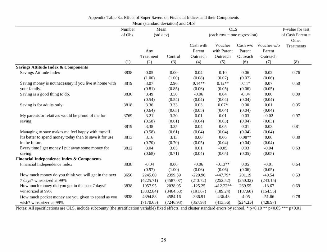
Last we examine several attitudinal indices, and child labor, in Table 7. Starting with the five attitudinal indexes, we note caution in interpretation: in theory, these may be either intermediate outcomes influenced directly by the treatment(s), or consequences of the shift in resources and test scores. In practice, we observe only two statistically significant shifts out of 20 estimates..
In terms of child labor, critics of financial education for youth posit that introducing children to savings and financial decision-making may have the unintended consequence of focusing their attention on income, and then discourage school attendance in order to work (Varcoe et al. 2005). Berry, Karlan and Pradhan (2013) tests this in Ghana with students of similar age as this study, and finds that a financial education curriculum along with a savings box (but no directive or facilitation of using the savings for education expenses) did lead to higher child labor, whereas if a social values component was added to the financial education curriculum, there was no impact on child labor. In our setting, we find no impact from the program on child labor, either hours worked or total wages. Overall, the estimates from Tables 6 and 7, combined with the other outcomes, indicate that the observed effects on learning occur solely through changes in available supplies rather than changes in attitude or participation.
Section VI. Conclusion
Weaker rather than stronger commitments can, in some instances, prove more effective. In the context of an educational savings program, we find that families and children save more under a weaker savings strategy in which funds are not dedicated to educational expenses upon deposit than they do under a strict commitment savings program in which all deposits are dedicated to educational expenses. The purpose of commitment savings devices is to intentionally limit the use of deposited funds. In some contexts, however, such services may need to strike a balance between providing sufficient limitations to make the savings mechanisms useful while being careful not to make the limitations so severe that they deter savings. Understanding the nature of this trade-off is an important direction for future research.
When combined with a parent sensitization program, we find that families and children spend their savings on educational expenses (school supplies). This does not, however, alter school participation – we find no effects on enrollment or attendance – but does improve students’ scores on a basic math and language test by 0.13 standard deviations. This suggests that financial constraints may play an important role in students’ academic performance and that understanding the role of families’ financial decision process may be an important element in understanding the overall production process of education.
On a practical level, several implementation issues are important to explore. As a program designed to improve student learning, treatment effects of this magnitude are large compared to other evaluations of interventions designed to provide resources to schools or directly to children (Jameel Poverty Action Lab 2014), but they are small relative to many other types of programs (most notably, for example, programs that provide additional resources while also changing
13
pedagogical strategies). Taking the programs relative low cost (2.24 USD per student per year) into account using the methodology proposed by Dhaliwal et. al.(2014), however, the program delivers learning gains at a cost of 1.49 USD per tenth of a standard deviation or 6.71 standard deviations per 100 USD.27 This is very competitive relative to other programs. Relative to the 27 studies compared by J-PAL (2014), only four produce improvements in test scores more cost-effectively.
In terms of encourage family savings, the program costs were high relative to the savings generated. However, if the program generated long term savings behavior change, then between the continued savings and the improvement in educational outcomes, it would surpass typical cost benefit calculations. In addition, it may be possible to reduce costs, particularly with implementation via mobile banking. This would obviate the need for physical transfer of cash to a bank, and would lower the risk of theft from keeping cash in a (albeit locked) box at the school. However, if the group nature of the intervention (i.e., the public and communal training) was an important element for take-up (through mimicking of peers, or learning from peers) and adherence (through monitoring and potential for social recognition), then a mobile banking implementation may lose that visual classroom element. Although these peer mechanisms were not emphasized in the training and implementation of the program, the fact that the savings were done publicly may have had such an effect.
On a more theoretical level, these results open up many related questions. Are external interventions of this sort effective in changing long term behavior, i.e., does the psychic cost of deviation persist, even without an outsider-led intervention? Did the intervention shift the preferences of the child, or the parents, or both, and what does this imply for intra-household cross-generational bargaining issues? How critical was the timing element of the “soft” commitment device, i.e., the fact that the school supplies were immediately available for purchase at the time of withdrawal? If that was critical, it is a ringing endorsement for the “make it easy” mantra, and also implies that the soft commitment device may have worked for reasons elaborated on in Mullainathan and Shafir (2013), because it increased the attention of individuals to educational expenses at exactly the right moment, when they had cash in their hands.
27 Estimates are provided in 2011 USD.
14
Figure 1: Research Timeline
2009 2010 2011
Term 1 Term 1 Term 1Term 2 Term 2 Term 2Term 3 Term 3 Term 3
Surveys:
Monitoring Visits:
Program
Activity
P
A
Y
O
U
T
P
A
Y
O
U
T
P
A
Y
O
U
T
P
A
Y
O
U
T
P
A
Y
O
U
T
P
A
Y
O
U
T
Savings:
Parent Sensitization:
Data Collected Baseline Endline
Parent sensitization treatment group
15
References
Ashraf, Nava, Dean Karlan, and Wesley Yin. 2006. “Tying Odysseus to the Mast: Evidence from a Commitment Savings Product in the Philippines.” Quarterly Journal of Economics 121 (2): 673–697.
———. 2010. “Female Empowerment: Further Evidence from a Commitment Savings Product in the Philippines.” World Development 38 (3): 333–344.
Avvisati, Francesco, Marc Gurgand, Nina Guyon, and Eric Maurin. 2013. “Getting Parents Involved: A Field Experiment in Deprived Schools.” The Review of Economic Studies (August 21): rdt027. doi:10.1093/restud/rdt027.
Barrera-Osorio, Felipe, Marianne Bertrand, Leigh Linden, and Francisco Perez-Calle. 2011. “Improving the Design of Conditional Transfer Programs: Evidence from a Randomized Education Experiment in Colombia.” American Economic Journal: Applied Economics 3 (2): 167–195.
Benabou, Roland, and Jean Tirole. 2004. “Willpower and Personal Rules.” Journal of Political Economy 112 (4): 848–887.
Berry, Jim, Dean Karlan, and Menno Pradhan. 2013. “Social or Financial: What to Focus on in Youth Financial Literacy Training?” Working Paper (June).
Clement, Douglas. 2013. “Interview with Richard Thaler.” The Region, September. Das, Jishnu, Stefan Dercon, James Habyarimana, Pramila Krishnan, Karthik Muralidharan, and
Venkatesh Sundararaman. 2013. “School Inputs, Household Substitution, and Teset Scores.” American Economic Journal: Applied Economics 5 (2): 29–57.
Dhaliwal, Iqbal, Esther Duflo, Rachel Glennerster, and Caitlin Tulloch. 2014. Comparative Cost-Effectiveness to Inform Policy in Developing Countries. Vol. forthcoming. University of Chicago.
Dupas, Pascaline, and Jonathan Robinson. 2013. “Why Don’t the Poor Save More? Evidence from Health Savings Experiments.” American Economic Review 103 (4) (June): 1138–1171. doi:10.1257/aer.103.4.1138.
Hidalgo, Diana, Mercedes Onofa, Hessel Oosterbeek, and Juan Ponce. 2013. “Can Provision of Free School Uniforms Harm Attendance? Evidence from Ecuador.” Journal of Development Economics 103: 43–51.
Independent Evaluation Group (IEG). 2007. “Fall out from the ‘Big Bang’ Approach to Universal Primary Education: The Case of Uganda”. World Bank. http://www.worldbank.org/oed/education/uganda.html.
Karlan, Dean, Aishwarya Ratan, and Jonathan Zinman. 2013. “Savings by and for the Poor: A Research Review and Agenda.” Review of Income and Wealth (October).
Kremer, Michael, and Alaka Holla. 2009. “Pricing and Access: Lessons from Randomized Evaluations in Education and Health.” In What Works in Development? Thinking Big and Thinking Small, edited by Jessica Cohen and William Easterly. Brookings Institution Press.
Mullainathan, Sendhil, and Eldar Shafir. 2013. Scarcity: Why Having Too Little Means so Much. New York: Times Books, Henry Holt and Company.
Murphy, Paul, Carla Bertoncino, and Lianqin Wang. 2002. “Achieving Universal Primary Education in Uganda: The ‘Big Bang’ Approach”. 24107. Education Notes. Washington, D.C.: The World Bank.
“Opportunities Lost: The Impact of Grade Repetition and Early School Leaving.” 2012. Global Education Digest 2012. UNESCO Institute for Statistics.
Piper, Benjamin. 2010. “Uganda Early Grade Reading Assessment Findings Report: Literacy Aquisition and Mother Tongue”. Makerere Institute for Social Research.
Shefrin, H., and R. Thaler. 1992. “Mental Accounting, Saving, and Self-Control.” In Choice Over Time. New York: Russell Sage Foundation.
Thaler, Richard H, and Cass R Sunstein. 2009. Nudge: Improving Decisions about Health, Wealth, and Happiness. New York: Penguin Books.
“Uganda Hits Universal Primary Education Target.” 2000. Newsletter of the World Education Forum in Dakar.
UN data. 2013. “Uganda”. United National Statistical Division. http://data.un.org/CountryProfile.aspx?crName=Uganda.
UNESCO. 2013. “Data Centre.” Institute for Statistics. http://www.uis.unesco.org/Pages/DataCentre.aspx.
Varcoe, Karen P., Allen Martin, Zana Devitto, and Charles Go. 2005. “Using a Financial Education Curriculum for Teens.” Journal of Financial Counseling and Planning 16 (1): 63–71.
Student Survey: Prefer 500 UGX today to 800 UGX next week
Student Survey: Child receives pocket money from family
Student Survey: Amount received in pocket money (UGX)
% of students in attendance: The enumerators count of the number of students present during a classroom visit, divided by the enrollment in the class as provided by the teacher.
Supplies Index: the normalized mean of 4 binary measures: whether a student has a uniform, notebook, mathset, and shoes. The coefficient is expressed as standard deviations
from the control mean. Attendance Code: A subjectively recorded code given with the enrollment data that indicates how frequently a student attends, from 1 (always attends) to
6 (never attends). OLS specifications: Columns 4 and Columns 5-8 include robust standard errors, clustered by school (the unit of randomization), and subcounty fixed effects
(the stratification variable). * p<0.10 ** p<0.05 *** p<.01
Table 1: Summary Statistics and Orthogonality Verification of Random Assignment, Full Sample Frame from Baseline
Mean (standard deviation) and OLS
Mean
(std dev) OLS (one specification per row)
Student Survey: Attendance Code (lower = more attendance)
Student Survey: Prefer 500 UGX today to 800 UGX tomorrow
Joint Significance Test F-stat, one regression per column with
Student Survey: Prefer 500 UGX today to 800 UGX next week
Table 2: Summary Statistics and Orthogonality Verification of Random Assignment, Post-Attrition Sample Frame
Mean (standard deviation) and OLS
Mean
(std dev) OLS (one specification per row)
Student Survey: Attendance Code (lower = more attendance)
% of students in attendance: The enumerators count of the number of students present during a classroom visit, divided by the enrollment in the class as provided by the
teacher. Supplies Index: the normalized mean of 4 binary measures: whether a student has a uniform, notebook, mathset, and shoes. The coefficient is expressed as
standard deviations from the control mean. Attendance Code: A subjectively recorded code given with the enrollment data that indicates how frequently a student attends,
from 1 (always attends) to 6 (never attends). OLS specifications: Columns 4 and Columns 5-8 include robust standard errors, clustered by school (the unit of
randomization), and subcounty fixed effects (the stratification variable).
* p<0.10 ** p<0.05 *** p<.01
Student Survey: Prefer 500 UGX today to 1,000 UGX next week
Student Survey: Child receives pocket money from family
Student Survey: Amount received in pocket money (UGX)
Student Survey: Total annual income from work (in 10,000
Results from bank administrative school-level data. Cumulative savings deposits for full two years of the program. Note that these data are collected at the school level,
i.e., the Average Deposits per Student is the average across schools of the average deposits per student at each school. * p<0.10 ** p<0.05 *** p<.01.
Table 3: Super Savers Program Savings by Treatment Group
Table 4: Process and Intermediate Outcomes, Intent to Treat Estimates
Mean (standard deviation) and OLS
Mean
(std dev)
OLS
(each row = one regression)
21
Table 4 Notes: Total Self Reported Savings (Endline Survey): sum of amount of money respondents reported savings in each of a variety of locations (at home
in local bank, hidden at home, give to a family member, savings program at school -- which likely includes the savings held as part of the treatment, in a bank
account of a family member, other). School Supplies Index (Classroom Visits): Enumerators at several classroom visits each term counted the number of
students with school supplies then we divided that number by the number of students in attendance. School Supplies Index (Endline Survey): the percentage of
students that have uniforms, notebooks, mathsets, and shoes. Parental Involvement Index includes 3 questions: 1) Student thinks parents are responsible for
children's education. 2) Has your parent come to your school in the past year? 3) Has your parent seen a report of yours from school in the past year? Savings
Attitude Index includes 7 statements each of which the student evaluated on a Likert scale, 1-5. All scales were converted after the fact so that higher on the
scale meant more positive attitude toward saving. 1) Saving money is not necessary if you live at home with your family. 2) Saving is a good thing to do. 3)
Saving is for adults only. 4) My parents or relatives would be proud of me for saving. 5) Managing to save makes me feel happy with myself. 6) It's better to
spend money today than to save it for use in the future. 7) Every time I get money I put away some money for saving. Column 5 compares the Cash with Parent
Outreach to the pool of the three other treatments and control group. OLS specifications: Columns 4-7 include robust standard errors, clustered by school (the
unit of randomization), a control for children's mean testing score, and subcounty fixed effects (the stratification variables). *p<0.10 **p<0.05 ***p<.01.
Column 8 is the p-value of an F-test of sigificance on a regression of the cash parent treatment against all other treatmnets and the same controls from Columns
Attendance Index 3586 -0.02 0.00 0.02 -0.00 -0.05 -0.03 0.23
(0.98) (1.00) (0.06) (0.06) (0.06) (0.06)
Panel B: Enrollment rate
2010 4716 0.44 0.44 -0.08 -0.03 -0.02 0.03 0.15
(0.50) (0.50) (0.05) (0.05) (0.05) (0.05)
2011 4716 0.24 0.22 -0.02 -0.00 0.02 -0.00 0.39
(0.43) (0.41) (0.04) (0.03) (0.04) (0.03)
P-value for test
of Cash Parent =
Other
Treatments
Attendance Rate: Based on a roll call of students on the official school enrollment list, counting only those students present in the class when roll call was
done. Attendance Index: includes 3 self-reported questions on student attendance: 1) Of the five school days of last week, how many were you absent? 2)
Think of a normal week from last term, of the five school days how many were you usually absent from school? 3) Think of a normal month from last
term, how many days were you usually absent? Enrollment Rate: Based on teacher responses as to whether a student on the official school enrollment list,
was still enrolled at that school. OLS specifications: Columns 4-7 include robust standard errors, clustered by school (the unit of randomization), a control
for children's mean testing score, and subcounty fixed effects (the stratification variables). *p<0.10 **p<0.05 ***p<.01. Column 8 is the p-value of an F-
test of sigificance on a regression of the cash parent treatment against all other treatmnets and the same controls from Columns 4-7.
Table 6: Effect of Super Savers on School Participation
Self Esteem Index: includes 10 statements each of which the student evaluated on a Likert scale, 1-5. All scales were converted after the fact so that higher on the
scale meant higher self esteem. 1) I am satisfied with myself. 2) Sometimes I think I am no good at all. 3) I believe I have a number of good qualities. 4) I am able to
do things as well as most children. 5) I do not have much to be proud of. 6) Sometimes I feel useless. 7) I believe I am a valuable person, at least as much as my
classmates. 8) I wish I could have more respect for myself 9) I sometimes think that I am a failure. 10) When I think of myself, I usually think good thoughts. In
addition to those 10 statements, there is one question: 11) Are you confident that you will be successful in the future? Time Preference Index: includes 2 hypothetical
time preference choices. 1) Would you rather receive 500 shillings today or 800 shillings next week? 2) Would you rather receive 500 shillings today or 1,000
shillings next week? From these, respondents were split into low, medium, and high future preference groups. Locus of Control: If a person is successful in life, is it
because he or she was lucky or because he or she worked very hard? (1=yes, 2=no) Financial Independence Index: includes 3 questions: 1) How much money do you
think you will get in the next 7 days? 2) How much money did you get in the past 7 days? 3) How much pocket money are you given to spend as you wish?
Aspirations Index: includes 4 questions about academic and vocation aspirations: 1) If you graduate from primary school, will your life be better than if you hadn’t
graduated? 2) Do you think you will go to secondary school? 3) Do you think you will reach university? 4) What do you want to be when you grow up? (student
responded with career that requires higher education) Exchange rate: 2815 Ugandan Shillings per US dollar. OLS specifications: Columns 4-7 include robust standard
errors, clustered by school (the unit of randomization), a control for children's mean testing score, and subcounty fixed effects (the stratification variables). *p<0.10
**p<0.05 ***p<.01. Column 8 is the p-value of an F-test of sigificance on a regression of the cash parent treatment against all other treatmnets and the same controls
from Columns 4-7.
Table 7: Effect of Super Savers on Student Attitudes
Mean (standard deviation) and OLS
Mean
(std dev)
OLS
(each row = one regression)
Total annual income from work (10k UGX), wins. 99%
25
2010 2011 2012
Student Survey
Grades Covered P5, P6 P6, P7
Median age 12, 13 13, 14
Sample Size (Students) 4983 4059
Attendance Survey
Grades Covered P5, P6 P6, P7 P7
Median age 12, 13 13, 14 14
Sample Size (Students) 37874 29016 13681
Classroom Survey
Grades Covered P5, P6, P7 P5, P6, P7 P5, P6, P7
Median age 12, 13, 14 12, 13, 14 12, 13, 14
Sample Size (Classes) 406 408 340
Appendix Table 1: Data Collection Summary
26
Dependent variable:
Endline Survey
Completed
Endline Survey
Completed
Endline Survey
Completed
Endline Test
Completed
Endline Test
Completed
Endline Test
Completed
(1) (2) (3) (4) (5) (6)
Cash with Parent Outreach -0.002 -0.004 -0.02 -0.0004 -0.002 -0.04
F-test (p-value) of joint significance of the four treatment
assignments
All specifications are OLS, include subcounty (the stratification variable) fixed effects, and cluster standard errors by school. * p<0.10 ** p<0.05 *** p<.01
F-test (p-value) of joint significance of interaction terms of
Notes: All specifications are OLS, include subcounty (the stratification variable) fixed effects, and cluster standard errors by school. * p<0.10 ** p<0.05 *** p<0.01
Appendix Table 3a: Effect of Super Savers on Financial Indices and their Components
Mean (standard deviation) and OLS
It's better to spend money today than to save it for use
in the future.
Managing to save makes me feel happy with myself.
My parents or relatives would be proud of me for
saving.
Saving money is not necessary if you live at home with
your family.
How much pocket money are you given to spend as you
wish? winsorized at 99%
How much money did you get in the past 7 days?
winsorized at 99%
How much money do you think you will get in the next
Has parent seen a report from school in the past year? 3838 0.90 0.90 0.01 0.00 -0.02 -0.02 0.19
(0.30) (0.29) (0.02) (0.02) (0.02) (0.02)
Has your parent come to your school in the past year? 3838 0.71 0.71 0.00 -0.02 0.00 0.01 0.69
(0.46) (0.45) (0.03) (0.02) (0.03) (0.03)
Student thinks parents are responsible for education. 3838 0.72 0.70 0.02 0.01 0.04 0.02 0.96
(0.45) (0.46) (0.03) (0.03) (0.03) (0.02)
Aspirations Index & Components
Aspirations Index 3838 -0.01 0.00 -0.04 -0.03 0.03 -0.03 0.56
(1.04) (1.00) (0.06) (0.06) (0.04) (0.06)
Do you think you will go to secondary school? 3699 -0.05 0.00 -0.10 -0.03 0.00 -0.09 0.39
(1.11) (1.00) (0.06) (0.06) (0.04) (0.06)
Do you think you will reach university? 3057 -0.05 0.00 -0.05 -0.10* 0.00 -0.09 0.95
(1.04) (1.00) (0.06) (0.06) (0.06) (0.06)
3838 0.05 0.00 0.08 0.00 0.06 0.04 0.26
(0.94) (1.00) (0.05) (0.04) (0.05) (0.05)
3838 0.02 0.00 -0.04 0.05 0.01 0.02 0.09
(0.98) (1.00) (0.04) (0.05) (0.05) (0.04)
Attendance Index & Components
Attendance Index 3586 -0.02 0.00 0.02 0.00 -0.05 -0.03 0.23
(0.98) (1.00) (0.06) (0.06) (0.06) (0.06)
Of five school days of last week, was absent for 3585 0.75 0.70 0.13 0.07 0.04 -0.02 0.33
(1.33) (1.27) (0.11) (0.08) (0.09) (0.09)
3586 1.27 1.31 0.00 -0.01 -0.02 0.44
(1.48) (1.54) (0.08) (0.09) (0.10) (0.10)
3463 3.34 3.59 -0.27 -0.18 -0.37** -0.16 0.80
(3.13) (3.55) (0.17) (0.21) (0.17) (0.19)
P-value for
test of Cash
Parent = Other
Treatments
Notes: All specifications are OLS, include subcounty (the stratification variable) fixed effects, and cluster standard errors by school. * p<0.10 ** p<0.05 *** p<0.01
Appendix Table 3b: Effect of Super Savers on Academic Indices and their Components
Mean (standard deviation) and OLS
Think of a normal month from last term, how many days were
you usually absent?
In normal week from last term, how many days were you
usually absent from school?
What do you want to be when you grow up? (student responded
with career that requires higher education)
Mean
(std dev)
OLS
(each row = one regression)
If you graduate from primary school, will your life be better
I am satisfied with myself. 3812 3.20 3.21 -0.01 -0.01 -0.01 -0.02 0.98
(0.67) (0.64) (0.05) (0.04) (0.04) (0.05)
Sometimes I think I am no good at all. 3817 2.55 2.54 -0.05 0.01 0.01 0.03 0.09
(0.79) (0.77) (0.04) (0.05) (0.04) (0.05)
I believe I have a number of good qualities. 3800 3.14 3.19 -0.07 -0.08* -0.03 -0.04 0.68
(0.71) (0.69) (0.05) (0.05) (0.03) (0.05)
I am able to do things as well as most children. 3822 3.31 3.33 -0.05 -0.01 -0.03 -0.04 0.38
(0.62) (0.62) (0.03) (0.03) (0.04) (0.04)
I do not have much to be proud of. 3777 2.42 2.43 0.03 -0.07 -0.02 0.01 0.23
(0.77) (0.78) (0.05) (0.04) (0.05) (0.05)
Sometimes I feel useless. 3816 3.08 3.08 -0.05 -0.01 0.05 -0.02 0.05
(0.80) (0.81) (0.03) (0.04) (0.04) (0.04)
3808 3.25 3.28 -0.07* 0.01 -0.06 -0.04 0.34
(0.62) (0.64) (0.04) (0.04) (0.04) (0.04)
I wish I could have more respect for myself. 3755 1.96 1.94 0.03 -0.06 0.05 0.02 0.61
(0.62) (0.61) (0.04) (0.05) (0.04) (0.04)
I sometimes think that I am a failure. 3814 2.98 2.96 -0.03 0.04 -0.04 0.09** 0.11
(0.84) (0.86) (0.04) (0.04) (0.04) (0.04)
3828 2.96 2.98 -0.04 0.02 -0.10** 0.01 0.83
(0.81) (0.82) (0.05) (0.05) (0.04) (0.05)
3652 0.96 0.97 -0.01 -0.02** -0.01 -0.01 0.91
(0.21) (0.18) (0.01) (0.01) (0.01) (0.01)
Time Preference Index & Components
Time Preference Index 3828 2.05 2.07 -0.02 -0.02 0.00 -0.03 0.96
(0.83) (0.82) (0.04) (0.04) (0.04) (0.04)
3828 1.37 1.37 0.01 -0.01 0.01 -0.01 0.44
(0.48) (0.48) (0.02) (0.03) (0.03) (0.02)
2415 1.49 1.52 -0.05 0.00 -0.01 -0.03 0.31
(0.50) (0.50) (0.03) (0.03) (0.03) (0.03)
P-value for test
of Cash Parent =
Other
Treatments
Notes: All specifications are OLS, include subcounty (the stratification variable) fixed effects, and cluster standard errors by school. * p<0.10 ** p<0.05 *** p<0.01
Appendix Table 3c: Effect of Super Savers on Self Esteem and Time Preference Indices and their Components
Mean (standard deviation) and OLS
I believe I am a valuable person, at least as much as
my classmates.
Would you rather receive 500 UGX today or 1,000
UGX next week?
Would you rather receive 500 UGX today or 800
UGX next week?
Are you confident that you will be successful in the
future ?
When I think of myself, I usually think good thoughts.