LEISURE LUXURIES AND THE LABOR SUPPLY OF YOUNG MEN
Mark AguiarMark Bils
Kerwin Kofi CharlesErik Hurst
Working Paper 23552http://www.nber.org/papers/w23552
NATIONAL BUREAU OF ECONOMIC RESEARCH1050 Massachusetts Avenue
Cambridge, MA 02138June 2017
We thank Shirley Yarin and Hyun Yeol Kim for outstanding research assistance. We also thank Thomas Crossley, Matt Gentzkow, Patrick Kehoe, John Kennan, Pete Klenow, Alan Krueger, Hamish Low, Kevin Murphy, and Yona Rubinstein, as well as seminar participants at Berkeley, Board of Governors of the Federal Reserve, Boston University, Chicago, Columbia, Harvard, Houston, IIES Stockholm, LSE, Penn, Princeton, Stanford, UCL, UIC, Wharton, and the Federal Reserve Banks of Atlanta, Chicago and Richmond for helpful comments. The views expressed herein are those of the authors and do not necessarily reflect the views of the National Bureau of Economic Research.
NBER working papers are circulated for discussion and comment purposes. They have not been peer-reviewed or been subject to the review by the NBER Board of Directors that accompanies official NBER publications.
Leisure Luxuries and the Labor Supply of Young MenMark Aguiar, Mark Bils, Kerwin Kofi Charles, and Erik HurstNBER Working Paper No. 23552June 2017JEL No. D1,E24,J01,J2
ABSTRACT
Younger men, ages 21 to 30, exhibited a larger decline in work hours over the last fifteen years than older men or women. Since 2004, time-use data show that younger men distinctly shifted their leisure to video gaming and other recreational computer activities. We propose a framework to answer whether improved leisure technology played a role in reducing younger men's labor supply. The starting point is a leisure demand system that parallels that often estimated for consumption expenditures. We show that total leisure demand is especially sensitive to innovations in leisure luxuries, that is, activities that display a disproportionate response to changes in total leisure time. We estimate that gaming/recreational computer use is distinctly a leisure luxury for younger men. Moreover, we calculate that innovations to gaming/recreational computing since 2004 explain on the order of half the increase in leisure for younger men, and predict a decline in market hours of 1.5 to 3.0 percent, which is 38 and 79 percent of the differential decline relative to older men.
Mark AguiarDepartment of EconomicsPrinceton UniversityFisher HallPrinceton, NJ 08544-1021and [email protected]
Mark BilsDepartment of EconomicsUniversity of RochesterRochester, NY 14627and [email protected]
Kerwin Kofi CharlesHarris School of Public PolicyUniversity of Chicago1155 East 60th StreetChicago, IL 60637and [email protected]
Erik HurstBooth School of BusinessUniversity of ChicagoHarper CenterChicago, IL 60637and [email protected]
1 Introduction
Between 2000 and 2015, market hours worked fell by 203 hours per year (12 percent) for
younger men ages 21-30, compared to a decline of 163 hours per year (8 percent) for men
ages 31-55. These declines started prior to the Great Recession, accelerated sharply during
the recession, and have rebounded only modestly since.1 We use a variety of data sources to
document that the hours decline was particularly pronounced for younger men. These trends
are robust to including schooling as a form of employment. Not only have hours fallen, but
there is a large and growing segment of this population that appears detached from the labor
market: 15 percent of younger men, excluding full-time students, worked zero weeks over
the prior year as of 2016. The comparable number in 2000 was only 8 percent.
An obvious candidate for this decline in younger men’s hours is a decline in demand for
their labor, resulting in a corresponding reduction in their real wages. There is evidence that
declining demand for manufacturing and routine employment has contributed to a secular
decline in wages and employment rates for less educated workers.2 However, we show in
the next section that real wages of younger men have closely tracked those of their older
counterparts since 2000. This suggests that the greater decline in younger men’s hours is
not readily explained by a differential decline in labor demand for younger versus older men.3
We go in a different direction. We ask if innovations to leisure technology, specifically to
recreational computer and gaming, reduced the labor supply of younger men. Our focus is
propelled by the sharp changes we see in time use for young men during the 2000s. Comparing
data from the American Time Use Survey (ATUS) for recent years (2012-2015) to eight years
prior (2004-2007), we see that: (a) the drop in market hours for young men was mirrored
by a roughly equivalent increase in leisure hours, and (b) increased time spent in gaming
and computer leisure for younger men, 99 hours per year, comprises three quarters of that
increase in leisure. Younger men increased their recreational computer use and video gaming
by nearly 50 percent over this short period. Non-employed young men now average 520
hours a year in recreational computer time, sixty percent of that spent playing video games.
This exceeds their time spent on home production or non-computer related socializing with
friends. Older prime age men and women allocate much less time to computer and gaming
and displayed little upward trend in these activities.
An elemental question is whether increased computer use and gaming contributed to the
1Data, described fully below, are from the March CPS and exclude full time students.2See, for example, Autor et al. (2013), Charles et al. (forthcoming), and Charles et al. (2016).3In the next section we also discuss the possibility that younger men’s ”permanent-income wage” has
declined relative to their ”flow” wage because the return to their work experience has declined. Elsby andShapiro (2012) and Santos (forthcoming) stress this as a factor in hours supplied by younger men.
1
rise in younger men’s leisure and the corresponding decline in their market hours, or simply
reflected their response to working fewer hours due, say, to reduced labor demand. That
is, has improved leisure technology raised the return to non-market time and consequently
increased the reservation wage of younger men, or are we witnessing movement along a stable
labor supply curve? The idea that changes in household technology shifts the labor supply
curve has a rich history in the literature on increasing female labor force participation. Our
focus is on the role leisure technology plays in the decline of male employment.
To identify shifts in the labor supply curve from movements along a stable labor supply
curve, we introduce a leisure demand system that parallels that typically considered for
consumption expenditures. In particular, we estimate how alternative leisure activities vary
with total leisure time, tracing out “leisure Engel curves.” Our estimation exploits state-year
variations in leisure, such as that caused by differential impact of the Great Recession across
US states. The key identifying assumption is that variations in total leisure at the state level
are not driven by differential changes in preferences or technologies across leisure activities.
We estimate that gaming and recreational computer use is distinctively a leisure luxury
for younger men, but not for other demographic groups. In particular, a one percent increase
in leisure time is associated with a more than 2 percent increase in time spent playing video
games for younger men. Watching TV has an elasticity slightly above one, making it a
modest luxury for younger men, while all other leisure activities have elasticities less than or
equal to one for younger men. This implies that any marginal increase in leisure for younger
men will be disproportionately devoted to computers and gaming.
With the estimated leisure demand system in hand, we quantify the change over time
in the marginal return to leisure based on how leisure’s allocation shifted across activities.
Specifically, we decompose the large increase in recreational computer use between 2004 and
2015 into a movement along the leisure Engel curve due to additional leisure time, and the
shift of the expansion path due to technological improvement in computer and video games
relative to other leisure goods. The estimated Engel curves are what allow us to identify
the increase in recreational computing and video gaming due to more free time from that
induced by a shift in the relative quality of the activity. From this decomposition, we infer
how much the marginal return to leisure increased over time due to improved computer and
video gaming technology. We also document that the relative increase in technology for
computer leisure and video gaming implied from our leisure demand system is consistent
with the relative price decline for computer and video game goods seen in BLS data.
The estimates from the leisure demand system establish that younger men experienced
an increase in the marginal return to leisure. To the extent that agents are on their labor
supply curve, that is, either close to the employment/non-employment margin or with the
2
ability to adjust on the intensive margin, the higher return to leisure will translate into a
shift in labor supply at a given wage. The next step in our analysis is to quantify this shift.
The mapping from improved technology to labor supply depends on how reduced earnings
affects consumption. We consider two scenarios. If individuals are “hand-to-mouth,” so
consumption equals labor earnings, we calculate that improvements in computer leisure
since 2004 were sufficient, holding wages fixed, to explain a 1.5 percent decline in the market
hours of younger men. Alternatively, if the marginal utility of consumption is held constant,
which in our framework holds a dollar’s marginal value constant, then the impact is twice
as large, yielding a 3.0 percent decline in market work for younger men. These declines
in hours, 1.5 to 3.0 percent, translate to 23 to 46 percent of the decline in market work
observed for younger men from 2004 to 2015. So we conclude that better leisure technology
was a significant factor, though not necessarily the primary factor, in the decline in hours
for younger men. We also find that increased computer technology has no effect on the
labor supply of older men and only a small effect on the labor supply of younger women.
Collectively, these findings imply that increased computer and video game technology can
explain between 38 and 79 percent of the differential decline in hours between younger and
older men during the 2000s.
An assumption that younger men’s consumption is held constant aligns with several pieces
of data. More generally, a natural question is how these younger men support themselves
given their decline in earnings. We document that 67 percent of non-employed younger men
lived with a parent or close relative in 2015, compared to 46 percent in 2000. The importance
of cohabiting with parents has been emphasized in the business-cycle context by Kaplan
(2012) and Dyrda et al. (2012). We document that it is also relevant for the longer-run
decline in employment of younger men. We also compare expenditures for households that
contain younger men to expenditures for all households, scaled appropriately for household
size. (Data are from the Panel Study of Income Dynamics.) By this measure, we see little,
if any, decline in the relative consumption of younger men since 2000.
Our narrative emphasizes the impact on labor supply of expanded leisure opportuni-
ties. An alternative is that younger men face diminished market opportunities. One avenue
to gauge how younger men perceive their fortunes is to use survey data on happiness. In
this spirit, we complement the patterns in hours, wages, and consumption with data on
life satisfaction from the General Social Survey. We find that younger men reported in-
creased happiness during the 2000s, despite stagnant wages, declining employment rates and
increased propensity to live with parents/relatives. This contrasts sharply with older men,
whose satisfaction clearly fell, tracking their decline in employment. We see this as suggestive
of a role for improved leisure options for younger men.
3
One major innovation in the mid 2000s was taking social interactions in general, and
video gaming in particular, online. Facebook, started in 2004, grew from 12 million users in
2006 to 360 million by 2009. Likewise, a generation of new video game consoles introduced in
2005 and 2006 allowed individuals to interact with others online.4 Massive multiplayer online
games launched around the same time. For example, World of Warcraft started in 2004 and
grew to 10 million monthly subscribers by 2010. These games allowed individuals to play at
their computer, requiring no separate video game console. The ability to interact with others
online, coupled with advances in graphics and access, led to a large expansion of the video
game industry during the mid-2000s.5 The timing of these technological advances coincided
with the period surrounding the Great Recession, making it difficult to separate the impact
of the Great Recession from the technological progress in computing using time series data
alone. Our structural model of leisure demand is designed to overcome this obstacle.
Our focus on time allocation owes a natural debt to the seminal papers of Mincer (1962)
and Becker (1965), which emphasize that labor supply is influenced by how time is allocated
outside of market work. We introduce the concept that some non-market activities are leisure
luxuries, which display little diminishing returns. Because recreational computer use and
video gaming is such a leisure luxury for younger men, we should expect improvements in
its technology to bring forth large increases in its time allocation.
Our work complements that of Greenwood and Vandenbroucke (2008), Vandenbroucke
(2009), and Kopecky (2011), who use a quantitative Beckerian model to show that declining
relative prices of leisure goods can help explain employment declines over the last century.
We augment this approach by considering a leisure demand system and exploring how the
allocation of time across leisure activities may also be relevant for labor supply. We show that
it is key for labor supply whether innovations affect leisure luxuries or leisure necessities.6
The paper is organized as follows: Section 2 documents declines in employment, hours
and wages for younger men and other demographic groups; Section 3 examines changes in
time use during the 2000s, emphasizing the dramatic increase in computer and video game
time for younger men; Section 4 presents our methodology including the leisure demand
system; Section 5 estimates the leisure Engel curves; Section 6 uses the demand system and
changes in time allocation to infer changes in leisure technology; Section 6 also quantifies the
4Microsoft released their Xbox 360 video game consoles in 2005, while Sony and Nintendo released theirPlaystation 3 and Wii consoles, respectively, in 2006. All three of these video game consoles allowed indi-viduals to interact with other players online.
5According to industry statistics, total nominal revenues of the video game industry increased by around50 percent between 2006 and 2009 after being roughly flat for the prior five years. Data are from the NPDgroup. See vgsales.wikia.com/wiki/NDP_sales_figures.
6This distinction for leisure’s response parallels that consumption’s inter-temporal elasticity hinges onthe share of goods with little curvature in consumption, emphasized by Browning and Crossley (2000).
shifts in leisure and labor supply curves for different demographic groups during the 2000s;
Section 7 highlights the robustness of our results to alternate parameterizations; Section 8
documents patterns in cohabitation, consumption, and self-reported well being for younger
men; and Section 9 concludes.
2 Background Labor Market Trends
In this section, we document labor market changes for younger men compared to other
demographic groups during the 2000s. Our primary data for trends in employment, hours,
and wages are the March Current Population Survey (CPS).7 We restrict the sample to
civilians ages 21 to 55. We further exclude full-time students who are less than age 25.8
This mitigates any role for increased college attendance in the decline in work hours for
younger men. We focus on two age groups: ages 21-30 (younger) and ages 31-55 (older).
Especially since we drop full-time students, the vast majority of the younger men sample (∼75 percent) has less than a college bachelor’s degree. Using only the small sample of more
educated men introduces a fair amount of sampling error, particularly in the time-use survey
used later in the paper. We therefore focus in the text on all younger men as our benchmark
as well as report results for the sub-sample with less than a college degree.
2.1 Employment and Hours Worked
Figure 1 reports work hours for younger and older men since 2000 based on the March CPS.
Panel (a) reports the log change in annual hours since 2000.9 Panel (b) reports employment
rates at the time of the March CPS survey. Annual hours decline over this period for both
younger and older men. But the decline is more severe for younger men. The separation
begins in the mid-2000s, accelerates during the Great Recession, and then fails to close
completely after the recession. Similarly in Panel (b), the employment rate of younger men
displays a sharper downward trend since 2000. From 2000 to 2016, the employment rate for
younger men fell by 8 percentage points, compared to 4 percentage points for older men.10
Table 1 Panel (a) reports the level of annual hours worked for men and women at four
7A Data Appendix accompanies the paper, providing greater discussion of all data sets, including yearlysample sizes. Throughout the paper, we weight observations by the relevant survey’s sampling weight.
8Between 1986 and 2012, the CPS asked only those under age 25 about school attendance.9For year t, annual hours are computed from year t+ 1’s March survey response regarding the previous
calendar year’s weeks worked times the response regarding usual hours worked per week the previous year.10Given the time frame, some of the younger men at the start of the period are part of the older sample
by the end. Appendix Figure A1 plots annual hours by age for various birth cohorts to provide a completepicture of how recent cohorts work fewer hours than the preceding cohorts at similar stages of the lifecycle.
Note: Data are from CPS March supplements. Full-time students less than age 25 are excluded.Panel (a) shows log hours relative to year 2000 for men ages 31-55 (squares) and ages 21-30(triangles). Annual hours equal last year’s weeks worked multiplied by usual hours worked perweek. The point for year t on the horizontal axis corresponds to responses from March t+ 1 reportof previous year’s hours. Panel (b) depicts employment rates at the time of the March survey forthe year indicated on the horizontal axis.
6
points over the last 15 years. Panel (b) reports the same for those with less than a college
degree. From 2000 to 2015, annual hours worked by younger men declined by 203 hours (12
log points) while the decline for OM was 163 hours (8 log points). The relative decline of
younger men versus older men is starker when we restrict attention to less educated men in
Panel (b). Younger less educated men experienced a 242 hour per year decline in market
work between 2000 and 2015 (a 14.4 log point decline). Table 1 also indicates that both
younger and older women experienced a decline in market work during the 2000s. However,
the declines were approximately one-third to one-half of their male counterparts. Younger
men in general and less educated younger men in particular experienced by far the largest
decline in hours worked during the 2000s relative to other sex-age-skill groups.
Figure 2 plots the fraction of younger and older men who worked zero weeks over the
year. This provides perspective on the extent that men of differing ages remain persistently
non-employed. Our sample continues to exclude full-time students ages less than 25. The
fraction reporting zero weeks worked is roughly similar at 8 percent across age groups in
2000. The fraction not working increased considerably during the 2000s for both groups;
but the increase is much more dramatic for younger men. The fraction of younger men not
working the entire year began increasing prior to the Great Recession, accelerated during
the Great Recession, and has only modestly recovered. As of 2015, the fraction of younger
men not working the entire year was nearly 15 percent.
Figure 2: Fraction of Men With Zero Weeks Worked Over Prior Year by Age, March CPS
Note: The figure shows the shares of men ages 31-55 (squares) and men ages 21-30 (triangles)who report working zero weeks during the prior year. Data are from the CPS March supplement.Full-time students ages less than 25 are excluded.
Note: Data are from the March CPS. Annual hours equal last year’s weeksworked multiplied by usual weekly hours. Year t hours refer to hours workedby year t+ 1 respondents. Full-time students less than age 25 are excluded.
8
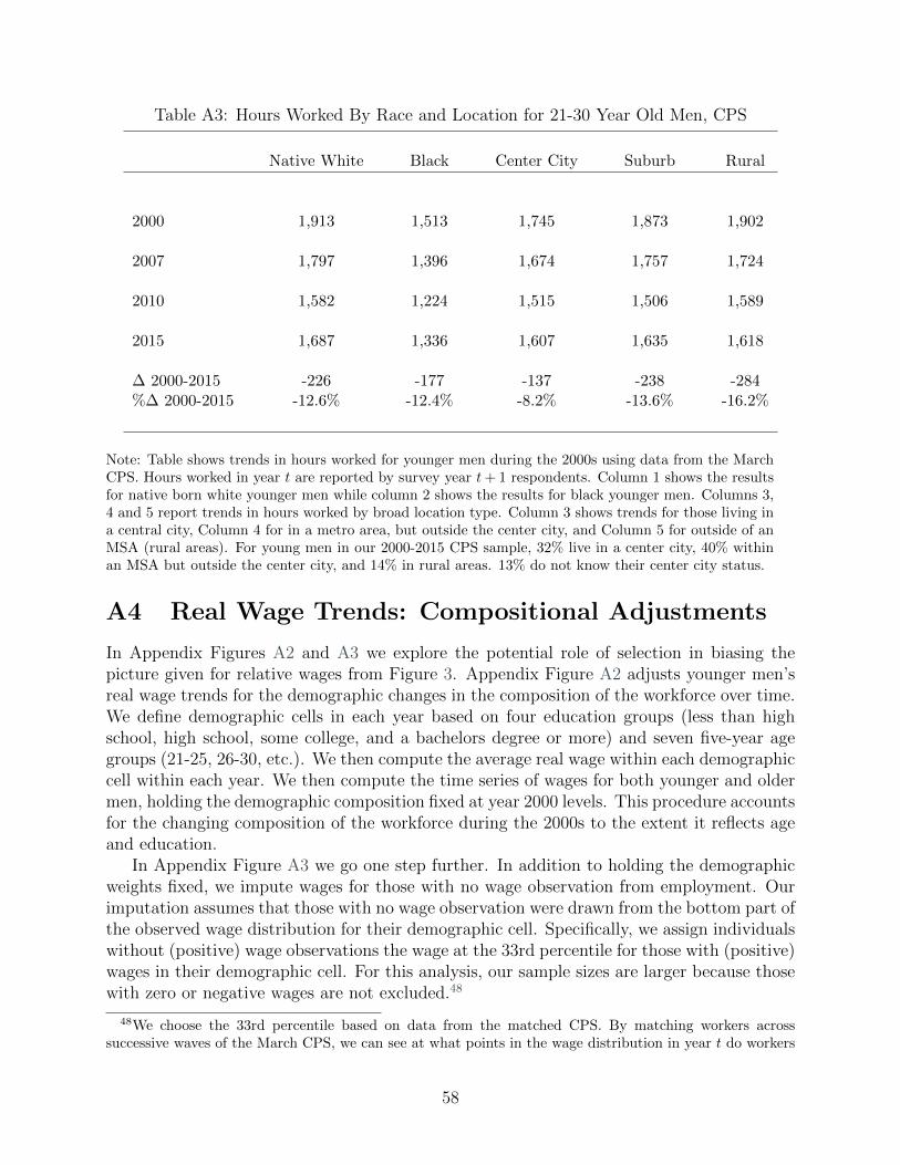
In the paper’s online appendix we perform a variety of robustness exercises. For example,
we extend the patterns in Figures 1 and 2 back through earlier recessions. While younger
men’s hours were always more cyclical, the large and persistent hours differences between
younger and older men is particular to the 2000s. Our robustness specifications also show
that the the decline in hours worked for younger men relative to older is a broad based
phenomenon, found in different surveys and across races. For example, we document similar
patterns in the Census and American Community Surveys (ACS). Beyond reinforcing results
from the CPS, these data allow us to explore robustness to excluding all full-time students,
including those more than 25 years old. Our results are not affected by excluding these older
students, as one might expect, given that full-time students are a small fraction of those ages
26-30. We also document that the patterns in Figures 1 and 2 hold similarly for white and
black households and across differing locations (center cities, suburbs, and rural areas).
2.2 Real Wages
In this subsection we document how real wages evolved in conjunction with the declines
in younger men’s hours reported above. We construct wages for year t based on year t + 1
March CPS data by dividing labor income for the prior year by the prior year’s annual hours.
We deflate this series by the June CPI-U. Wages are computed for those in our CPS sample
that report positive earnings. After imposing this restriction, we trim the top and bottom
one percent of the wage distribution in each year.
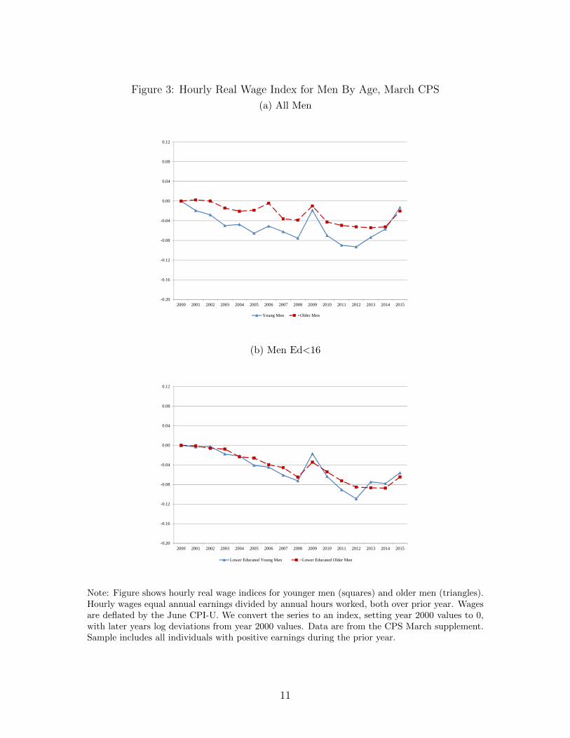
Figure 3 reports the log difference in real wages since 2000. Panel (a) is the full sample
of men, while Panel (b) restricts attention to those with less than 16 years of schooling.
Real wages decline over this period in all cases. However, unlike market hours, the decline
for younger men tracks that of older men closely, particularly for less educated men. One
caveat is that our wage series is constructed from repeated cross sections. It is well known
that changes in composition of the workforce over time can bias trends in such series. In
the online appendix we explore a number of alternatives to address this challenge.11 These
adjustments suggest a larger decline in real wages since 2000, but still indicate no difference
in wage trends between younger and older men.
The declines in hours and wages documented in this section surely reflect a combination
of factors. Many authors have highlighted a role for declining labor demand, especially for
workers with less schooling.12 The sharper decline in relative hours of younger men, given a
11In particular, we adjust wages for demographic changes in composition. We also impute wages for thosenon-employed using the 33rd percentile of the wage distribution for their demographic group.
12See Autor et al. (2003), Moffit (2012), Autor and Dorn (2013), Autor et al. (2013), Hall (2014), Charleset al. (forthcoming), Charles et al. (2016), and Acemoglu et al. (2016). Collectively, these papers provideevidence – often by exploiting cross-region variation – that declining labor demand has been an important
9
similar decline in their real wages, suggests a possible role for younger men’s labor supply,
either in terms of a high responsiveness to contemporaneous wage changes or shifts in their
willingness to work. Understanding the evolution of younger men’s labor supply over the
past fifteen years is the focus of the paper.
Working contributes to permanent income, not only through today’s wage, but also
through any impact of work experience on future wages. Elsby and Shapiro (2012) and
Santos (forthcoming) each point to reasons the investment return to working may have
fallen in recent years. Elsby and Shapiro (2012) stress that a decline in trend wage growth,
by flattening age-earnings profiles, has devalued the expected return on work experience. If
the wealth effect of this change on labor supply is sufficiently weak, this will raise reservation
wages, especially for younger workers. Santos (forthcoming) estimates that the impact of
working on future earnings has lessened for low wage workers. This acts to raise reservation
wages for these workers, especially younger low-wage workers. Our work complements these
papers by showing that innovations to computer leisure also raised the reservation wage
for younger men. Because younger men are predicted to respond more to these leisure
innovations, our findings also help to explain the sharp divergence in work hours between
younger and older men that started in the mid-2000s.
3 The Changing Composition of Leisure
We first document how younger men, and other demographic groups, have allocated their
non-market time since the early 2000’s. We do so using the time diaries of the American
Time Use Survey (ATUS) from 2004 through 2015.13 Our ATUS sample is discussed in
detail in the Data Appendix. Briefly, the ATUS draws a sample from CPS respondents and
surveys them within a few months after the final CPS survey, collecting a 24-hour time diary
in which the respondent records the previous day’s activities in 15-minute intervals. These
activities are categorized into detailed activity codes by the ATUS. The sample is drawn
such that each day of week is equally represented. Our ATUS sample restrictions are the
same as for the CPS sample used in the previous section; in particular, we exclude full-time
students less than age 25.
factor for regional variation in wages and employment rates, with the effects concentrated among prime-ageless-educated workers.
13Though the ATUS starts in 2003, we begin our analysis with 2004, as there are small changes in thesurvey methodology between 2003 and 2004.
10
Figure 3: Hourly Real Wage Index for Men By Age, March CPS
Note: Figure shows hourly real wage indices for younger men (squares) and older men (triangles).Hourly wages equal annual earnings divided by annual hours worked, both over prior year. Wagesare deflated by the June CPI-U. We convert the series to an index, setting year 2000 values to 0,with later years log deviations from year 2000 values. Data are from the CPS March supplement.Sample includes all individuals with positive earnings during the prior year.
11
3.1 Trends in Broad Time Use Categories
We begin by aggregating activities into six broad categories: market work, job search, home
production, child care, education, and leisure. Job search includes such activities as sending
out resumes, job interviewing, researching jobs, or looking for jobs in the paper or the In-
ternet. Home production includes time doing household chores, preparing meals, shopping,
doing home or vehicle maintenance, and caring for other adults. We record child care sepa-
rately from home production. Education refers to time spent on one’s own education, such
as time attending courses, or doing related homework. Leisure consists of watching televi-
sion and movies, recreational computing and video games, reading, playing sports, hobbies,
etc. We discuss leisure in more detail in the next subsection. We include a sub-set of time
spent on eating, sleeping, and personal care (ESP) in leisure. In particular, we treat 7 hours
per day as non-discretionary ESP, and the residual as leisure.14 Transportation time spent
traveling to or from an activity is always included in the activity’s time. We report time use
in “hours per week” by multiplying the daily average by 7.
Table 2 shows time use for younger and older men (Panel a) and younger and older women
(Panel b) during the 2000s. To increase power we group together data for 2004-2007 and for
2012-2015. In additional to reporting the average levels of time use in each time period, we
also report differences across the two periods. Starting with the top panel, we see that both
younger men and older men reduced their market work over this time period, respectively,
by 2.5 and 1.2 hours per week. Multiplying by 52 weeks to obtain an annualized measure,
the ATUS indicates that younger men reduced weekly labor hours by 68 hours more than
older men, a difference slightly larger than that obtained from the CPS.
Comparing the top and bottom row of Table 2 Panel (a), we see that the declines in
market hours are nearly matched by associated increases in leisure for both younger and
older men. The remaining activities reveal small changes that approximately net out to
zero. Thus, the relative decline in labor hours for younger men is matched by a relative
increase in leisure, a differential increase on the order of 1.3 hours per week, or nearly 58
hours per year.
Panel (b) shows patterns for women. Younger women had a smaller decline in market
work, but a larger decline in home production, than younger men. On net, younger women
experienced a smaller increase in leisure than younger men. The decline in home production
for women during this periods reflects a well known trend that dates back at least a half
14Approximately 95 percent of respondents report 7 or more hours per day for ESP. We explored al-ternatives (such as 6, 8 or 9 hours per day) and found no sensitivity to the choice. In addition to thenon-discretionary ESP hours, we omit a few minor categories, such as own health and a catch-all ”uncate-gorized” activity code.
12
Table 2: Broad Time Allocation During the 2000s, Hours Per Week
Market Work 27.4 27.1 -0.3 27.4 27.0 -0.5Job Search 0.2 0.3 0.1 0.2 0.3 0.1Home Production 19.0 17.5 -1.5 24.2 22.4 -1.8Child Care 10.0 8.8 -1.2 7.4 7.6 0.2Education 2.3 2.9 0.6 1.1 1.0 -0.1Leisure 58.5 59.9 1.4 56.1 58.0 1.9Note: Table reports hours per week spent on different time use activities by age and sexfrom the ATUS. Data is shown for the pooled 2004-2007 and 2012-2015 periods. The differ-ence between the two periods is also shown. The individual’s total time endowment, aftersubtracting off the biological component of sleeping, eating and personal care, is 119 hoursper week. The table omits the time individuals spend on their own medical care as well astime use that the ATUS was not able to be categorized.
13
century (see Aguiar and Hurst (2007)). The decline in home production was even more
pronounced for older women, generating a larger increase in leisure than for younger women
or older men. Comparing across all demographic groups, younger men systematically have
the largest gain in leisure over this period.
3.2 Trends in the Nature of Leisure
We now explore leisure at a more disaggregated activity level. Within total leisure, we
distinguish the following five activities: recreational computer time; television and mov-
ing watching; socializing; discretionary eating, sleeping and personal care (ESP); and other
leisure. Recreational computer time includes time spent on non-work email, playing com-
puter games, surfing or browsing web sites, leisure time on smart phones, online chatting,
engaging in social media and unspecified computer use for leisure. We often highlight the
video/computer game component of recreational computer time.15 Computer time for work
or non-leisure activities (like paying bills or checking email) are embedded in other time-use
categories (like household management). Watching television and movies includes not only
watching traditional television and movie platforms, but also streaming platforms like Netflix
or youtube. Socializing includes entertaining or visiting friends and family, going to parties,
hanging out with friends, dating, and participating in civic or religious activities. “Other
leisure” includes all remaining leisure activities, such as reading, relaxing, listening to music,
going to the theater, exercising, playing sports, and engaging in hobbies.
Table 3 shows hours per week spent in each leisure category by younger men. The top
row repeats total leisure as reported in the bottom row of Table 2. We see that the increase
in leisure of 2.3 hours per week for all younger men is predominantly accounted for by a 1.9
hour per week increase in recreational computer time. Recreational computing and video
gaming represents 82 percent of the total leisure increase for all younger men. Most of this
increase took the form of increased video game playing (roughly 1.4 hours per week). This
99 hour per year increase in recreational computer use for young men is a very large change
in one time use category over a relatively short amount of time. For reference, the time spent
on home production for women fell by 520 hours per year over the last forty years (Aguiar
and Hurst (2007)). The complement of the large increase in computer time, is that other
leisure categories changed very little, despite the large increase in total leisure. For example,
younger men did not spend significantly more time watching TV/movies, socializing, or at
15The ATUS has a category of time use labeled “playing games”. This includes video games, but alsoincludes playing cards as well as traditional board games like checkers, Scrabble, etc. So we cannot distinguishplaying the Scrabble board game from video gaming. We document below that there was a very large increasein playing games during the 2000s, especially for younger men. We equate this with an increase in videogaming. However, we realize that we may be identifying a Scrabble boom as opposed to a video game boom.
14
other leisure activities. The only other leisure category that recorded a substantial increase
is eating, sleeping, and personal care, although in percentage terms the increase is quite
modest.
Table 3: Leisure Activities for Men 21-30, Hours per Week
Activity 2004-2007 2012-2015 Change
Total Leisure 61.0 63.4 2.3
Recreational Computer 3.3 5.2 1.9Video Game 2.0 3.4 1.4
Note: Table shows average weekly hours spent at leisure activities for men ages 21-30. These componentssum to total leisure time. The first column pools the 2004-2007 waves of the ATUS while the second columnpools the 2012-2015 waves. Video gaming is a subcomponent of total computer time. ESP refers to residualeating, sleeping and personal care.
Table 4 reports leisure patterns for younger men by employment status. Employed
younger men experienced a 2.0 hours-per-week increase in leisure over our sample period. 65
percent of this is accounted for by increased recreational computer time, with the bulk of that
increase spent playing video games. Not surprisingly, the non-employed have substantially
more leisure. However, conditional on non-employment, leisure hours actually fell since 2004.
This partly reflects a composition shift in the pool of non-employed, as non-employment now
constitutes a much bigger share of younger men. As seen in the last row of Table 4, the
non-employed in 2012-2015 were much more likely to allocate time to both education and
job search. These increases exactly offset the decline in leisure time. Nevertheless, despite
the overall decline in leisure time for non-employed younger men during the 2000s, time
spent on recreational computers (video games) increased for this group by 4.3 (2.5) hours
per week. It is also worth noting that in 2012-2015 non-employed young men spent nearly
10 hours per week (520 hours per year) on recreational computer activities. This exceeds
both the amount of time they spend socializing on non-computer activities and the amount
of time they spend on other leisure categories (exercise and sport, hobbies, relaxing, etc.).
The above average time spend on recreational computer activities for non-working younger
men masks a large amount of heterogeneity. For example, in 2004-2007 only 30 percent of
non-working younger men reported spending time on recreational computer time. The com-
parable number for 2012-2015 was 40 percent. Conditional on spending time on recreational
15
Table 4: Leisure Activities for Men 21-30 (Hours per Week): By Employment Status
Job Search and Education 2.0 1.9 -0.1 9.4 14.1 4.7Note: Table shows average hours spent per week across leisure activities for younger men by employmentstatus. Components sum to total leisure time. The first column of each panel pools data for the 2004-2007 waves of the ATUS. The second pools waves 2012-2015. Video gaming is a subcomponent of totalcomputer time. ESP refers to residual eating, sleeping and personal care.
computer activities, non-working younger men reported spending 2.6 and 3.4 hours per day
in the 2004-2007 and 2012-2015 periods, respectively. During the 2012-2015 period, 11 per-
cent of non-working younger men spent more than 4 hours per day at computer leisure, with
4 percent spending more than 6 hours. Thus, for some younger men, their primary activity
during the day was time spent at computer leisure.
To infer relative changes in computer leisure technology below we will exploit the fact
that individuals are shifting their leisure toward computer activities holding constant their
total leisure time. As a first look at the data, we sort individuals into bins based on the
amount of leisure enjoyed in the previous day. The bins are on the horizontal axis of Figure 4,
where, for example, the label 5 indicates that the individuals in the bin spent five to six hours
the previous day on leisure. For ease of presentation the units are hours per day rather than
hours per week. For each leisure bin, we average the amount of time allocated to recreational
computer use across individuals within the bin. The bars in the figure depict the averages
for younger men for the periods 2004-2007 (lighter bars) and 2012-2015 (darker bars). The
figure indicates that computer time has increased systematically within essentially all leisure
bins over the last fifteen years. Moreover, the increase has been particularly strong for high-
leisure individuals. For example, younger men with 9 to 10 hours of leisure per day tripled
computer time between 2004 and 2015, from 0.3 to 0.9 hours per day.
16
Figure 4: Younger Men’s Hours per Day of Computer Leisure by level of Total Leisure
0.0
0.2
0.4
0.6
0.8
1.0
1.2
1.4
1.6
1.8
2.0
<5 5 6 7 8 9 10 11 12 13 14 15+
Com
pute
r Tim
e (H
ours
Per
Day
)
Total Adjusted Leisure Time Bins (Hours Per Day)
Year: 2004-2007 Year: 2012-2015
Note: Figure shows average time spent on computer leisure (including video games) by individual’stotal leisure. Time use is expressed in hours per day. Except for first and last bins, leisure binsspan one hour per day, with minimal value of each bin denoted.
Figure 5: Younger Men’s Hours per Day of Computer Leisure by Leisure Quartile
0.0
0.5
1.0
1.5
2.0
2.5
3.0
1 2 3 4 1 2 3 4
Com
pute
r Ti
me
(Hou
rs P
er D
ay)
Year: 2004-2007 Year: 2012-2015
Adjusted Leisure Quartile:Working Men
Adjusted Leisure Quartile:Non-Working Men
Note: Figure shows average time spent on computer leisure (including video games) by total leisurequartile. Results shown separately by employment status–leisure quartiles are defined separatelyfor working and non-working men. Quartile thresholds are defined by the 2004-2007 distributionfor both periods. For working men the 25th, 50th, and 75th percentiles are 5.8, 8.3, and 12.9 hoursper day. For non-working men, these are respectively 9.7, 12.9, and 16.3.
17
Individual differences in total leisure largely reflect differences in market work. Figure
5 conditions on employment status. For this figure, we sort younger men into bins defined
by the quartile thresholds of the 2004-2007 distribution (for each employment status), using
the same bin thresholds for both periods.16 The higher leisure quartiles for working younger
men are disproportionately skewed towards individuals whose time diary day fell on a week-
end. Figure 5 shows that computer time increased for both employed and non-employed
younger men, holding constant total leisure. The increase was especially pronounced for
non-employed younger men.
Table 5 compares younger men’s shift toward computing and gaming to that for other
demographic groups. The top panel reports total leisure, computer leisure, and video game
time for younger men for 2012-2015 versus 2004-2007. The lower panels show the same for
older men, younger women, and older women. The table clearly shows that the increase in
computer leisure in general, and its gaming component in particular, was a younger men’s
phenomenon. While younger men increased their computer leisure by 1.9 hours per week,
the increases were only 0.1, 0.7, and 0.5 hours per week for older men, younger women, and
older women, respectively. Women reported a modest increase in their recreational computer
time; but, in contrast to younger men, zero of that increase involved video games.
4 Leisure Luxuries and Labor Supply
In this section we derive a leisure demand system that maps total leisure into specific leisure
activities. We show how observations on changing time allocations can be used to infer
shifts in the quality of leisure activities in general and changes in the marginal return to
total leisure in particular. The change in the marginal return can then be linked to shifts in
labor supply. This section develops the theoretical groundwork for the empirical estimation
in Section 5 and the quantitative results of Sections 6 and 7.
4.1 Preferences
Agents have preferences over a numeraire consumption good, c, and time spent on leisure
activities hi, i = 1, ..., I. We assume weak separability between consumption and leisure
activities. Utility can therefore be written U(c, v(h1, ..., hI ;θ)), where v is an aggregator
over leisure activities and θ = {θ1, ..., θI} is a vector of technology shifters.
16The specific quartile thresholds in hours per day are [0, 5.8), [5.8, 8.3), [8.3, 12.9), [12.9, 24] for employedyounger men and [0, 9.7), [9.7, 12.9), [12.9, 16.3), [16.3, 24] for non-employed younger men.
18
Table 5: Computer Leisure and Video Game By Age-Sex-Skill Groups, ATUS
(1) (2) (3)Pooled Pooled Diff
2004-2007 2012-2015 (2)-(1)
Men 21-30, Ed=All
Total Leisure 61.0 63.4 2.3Recreational Computer 3.3 5.2 1.9Video Games 2.0 3.4 1.4
Men 31-55, Ed=All
Total Leisure 57.0 58.1 1.1Total Recreational Computer 2.1 2.2 0.1Video Games 0.9 0.8 -0.1
Women 21-30, Ed=All
Total Leisure 58.5 59.9 1.4Total Recreational Computer 1.5 2.2 0.6Video Games 0.8 0.8 0.0
Women 31-55, Ed=All
Total Leisure 56.1 58.0 1.9Total Recreational Computer 1.6 2.1 0.5Video Games 0.6 0.7 0.1
Note: Table shows average hours spent per week in computer leisureand video gaming across age-sex-skill groups. The first column reflectsATUS waves 2004 to 2007, the second 2012-2015. Video game time is asubcomponent of computer leisure.
19
We assume v has the following functional form:
v(h1, ..., hI ;θ) =I∑i=1
(θihi)1− 1
ηi
1− 1ηi
. (1)
The parameter ηi > 0 is activity specific and governs the diminishing returns associated with
additional time spent on activity i. Increases in the technology parameter θi increase the
utility associated with spending a given amount of time at activity i.
While each leisure activity enters with its specific elasticity ηi, the activities are assumed
to be additively separable from one another (although the entire v function may be raised
to a power, which would be a feature of the overall utility function U). This assumption
implies that the marginal value of allocating time to one leisure activity is not dependent on
how leisure time is allocated across the other activities. We provide some empirical support
for this assumption in Section 5.
4.2 Leisure Engel Curves
For expositional purposes, we solve the agent’s problem in two stages. In the “first” stage,
the agent chooses c, allocates a unit of time between leisure time H and market labor 1−H,
and purchases a technology bundle θ. In the “second” stage, the agent allocates H across the
I activities. The first stage choices depend on wages, income, and the prices of alternative
technology bundles. The only price in the second stage is the shadow cost of time given H.
Working backwards, we consider the second stage budgeting problem in this subsection and
then return to the first stage in the next.
The second stage problem is:
v(H;θ) ≡ max{hi}Ii=1
v(h1, ..., hI ;θ)
subject to∑i
hi ≤ H.
Let µ denote the multiplier on the total leisure constraint. The first-order conditions are:
θ1− 1
ηii h
− 1ηi
i = µ. (2)
The parameter ηi is the elasticity of activity i with respect to leisure’s shadow price, µ.
20
Taking (2) and imposing the time constraint, which holds with equality, we have:
H =∑i
θηi−1i µ−ηi . (3)
Given H, there is a unique positive solution µ to (3). The envelope condition implies that
v′(H;θ) ≡ ∂v/∂H = µ, and v is strictly concave in H.
A focus of our empirical work is how marginal leisure time is allocated across activities.
The leisure Engel curve for activity i traces out how hi varies with total leisure time, H.
This is directly analogous to traditional expenditure Engel curves. Define βi as the elasticity
of hi with respect to H, holding constant θ. The first-order conditions imply:
βi ≡d lnhid lnH
∣∣∣∣θ
=ηiη, (4)
where η ≡∑
i siηi is a weighted average of elasticities ηi, with weights si = hi/H given
by activity i’s share of total leisure time. For convenience, we write si, βi, and η without
explicitly indicating that they depend on H and θ. The reader should keep in mind that they
are not parameters but outcomes of the agent’s optimization and, save for the knife-edge
case of identical ηi = η,∀i, will vary with the state variables.
From equation (4), the elasticity of hi with respect to H is the activity’s own elasticity
with respect to v′(H;θ) divided by the weighted average of all elasticities. Activities with
a greater ηi increase disproportionately with total leisure. That is, high ηi activities are
“leisure luxuries.” Our notion of a leisure luxury parallels the notion of a consumption
luxury good in traditional models of consumption demand systems.
With the leisure Engel curves, we can link shifts in time spent across activities to an
implied change in the marginal utility of total leisure. Let I denote the activity of interest,
which in the empirical analysis will be recreational computer use and video games. Let j 6= I
be a “reference activity.” In the empirical implementation, we consider several alternatives
as the reference. From the respective first-order conditions (2), we have:
ln θ1− 1
ηII − ln θ
1− 1ηj
j =lnhIηI− lnhj
ln ηj= η−1
I
(lnhI −
βIβj
lnhj
), (5)
where the second equality uses the definition of β from equation (4).
Now consider two allocations (H,θ), with associated (hj, hI). Differencing (5) across the
21
two allocations, we have:
∆ ln θ1− 1
ηII −∆ ln θ
1− 1ηj
j = η−1I
(∆ lnhI −
βIβj
∆ lnhj
). (6)
Note that βI/βj = ηI/ηj does not depend on H or θ and so is held constant.
Our derivation of the leisure Engel curves and the expression for technology change,
equation (6), do not hinge on how total hours of leisure H are determined. For instance,
they hold for changes in total leisure that correspond to declines in home production as well
as those that correspond to declines in market work. Similarly, they hold for variations in
total leisure associated with changes in market work at the extensive, employment margin
as well as those at the intensive, hours margin. In fact, these equations hold even if the
individual cannot choose total leisure versus work, perhaps due to rigidities in the labor
market.
Equation (6) will play an important role in our empirical analysis. To gain intuition for
how technology can be inferred from time allocations, consider the term in parentheses on the
far right of equation (6). This term is ∆ lnhI , minus the percent change in hI that one would
predict based solely on how time spent on activity j has changed, assuming technologies
were constant. Any deviation is then attributed to changes in technology. In particular,
suppose we observe data that indicates a change from (hj, hI) to (h′j, h′I). This change can
be partially due to total leisure moving from H to H ′. That component represents relative
movements along the activities’ leisure Engel curves, with the relative movement captured
by the difference in slope parameters βI and βj. Any residual movement represents a relative
shift in the leisure Engel curves–that relative shift in Engel curves reveals the movements in
θI versus that in θj. Hence, given knowledge of the leisure Engel curves, we can attribute
the changing patterns of time use between movements along Engel curves and changes in
technology. With this procedure, in Section 6 we will use our estimated βi (from Section 5)
and observed shifts in time allocation (from Section 3) to measure the relative increase in
technology for computers and video games.
4.3 The Decisions for Leisure Technology and Labor Supply
We now turn to the agent’s ”first” stage problem of choosing a technology bundle θ together
with an allocation of time between work and total leisure. For simplicity, we do so in a static
setting in which the agent faces a wage rate w and an endowment of non-labor income y.
We model the choice over θ as follows. For each activity i, the agent faces a menu of
θi ∈ [0, θi] with a price schedule pi(θi). Specifically, by paying pi(θi), the agent purchases a
22
bundle of inputs that yield a technology parameter θi. We assume pi is weakly increasing,
differentiable, and weakly convex. For computers and video games, a natural interpretation is
that the bundles are combinations of consoles and games of a particular vintage. Consumers
have the option of purchasing the state-of-the-art package at pi(θi), or a previous vintage at
a cheaper price. Technological progress is viewed as an increase in θi. Denote the choice set
for the vector of technologies Θ ≡ Πi[0, θi]. The individual’s problem is then:
maxc,H∈[0,1],θ∈Θ
U(c, v(H;θ)) (P)
subject to
c+∑i
pi(θi) ≤ w(1−H) + y.
A necessary optimality condition for interior H and c is:
Uvv′(H;θ) = wUc, (7)
which is our version of the familiar consumption-leisure tradeoff. Throughout the analysis
we shall assume that H is interior and hence equation (7) holds with equality.17
For the choice of θi, the necessary condition for an interior optimum is:
Uv∂v
∂θi= p′i(θi)Uc. (8)
For θi = θi, the equal sign is replaced with ≥. Conversely, for θi = 0, the equal sign is
replaced with ≤.
It is convenient to define the elasticity of price with respect to quality:
φi(θi) ≡d ln pi(θi)
d ln θi.
We can use (7) to substitute for Uv/Uc in (8) to write the first-order condition for an interior
17Keep in mind that the analysis of the sub-problem in the preceding section does not rest on (7) holdingwith equality. In particular, that analysis is independent of whether employment is divisible or not. Weuse equation (7) to trace out how a technological change that shifts the marginal utility of leisure affectsthe choice of H. If employment is chosen on the extensive margin, we need to interpret the response asthe fraction of the population of interest that chooses to work, rather than the fraction of time for a singleindividual.
23
θi as:18
φi(θi) =whipi(θi)
. (9)
This says that a higher sensitivity of price to quality induces the agent to shift the cost of
activity i towards time and away from the market input.
The Frisch elasticity of leisure is the elasticity of leisure with respect to the wage holding
constant the marginal utility of consumption (and θ):
ε ≡ −d lnH
d lnw
∣∣∣∣Uc,θ
. (10)
This elasticity depends on the sensitivity of Uv as well as v′(H;θ) to movements in H. From
(2), we have
d ln v′(H;θ)
d lnH
∣∣∣∣θ
= − 1
ηi
d lnhid lnH
= −βiηi
= −1
η.
Let σ ≡ −d lnUvd lnH
. Differentiating (7) yields the following:
1
ε=
1
η+ σ. (11)
Thus the Frisch elasticity reflects both the average curvature over individual leisure activities
(η−1) and the curvature over the leisure bundle (σ). As noted above, η varies with H, and
hence the Frisch elasticity is not a constant structural parameter.19 In particular, as H
increases, the shares devoted to high-η luxuries increase, which from (11) raises the Frisch
elasticity of leisure for a given σ.
4.4 The Response of Labor Supply to Leisure Technology
We now consider the impact of technology on labor supply. In particular, we are interested
in how an improvement in θI influences the choice of H. As θI is a choice variable, one
natural interpretation of the comparative static is an increase in the technological frontier,
18Specifically, in equation (8), replace Uv/Uc with w/vH from equation (7). The envelope condition forthe leisure sub-problem implies vθi/vH = hi/θi. Substituting into (8), we have whi = θip
′(θi) = pi(θi)φi(θi).19There are close antecedents to this result in the literature on consumption. In particular, Crossley and
Low (2011) discuss the restrictions necessary for a constant elasticity of inter-temporal substitution in ademand system involving multiple consumption goods. Browning and Crossley (2000) demonstrate the linkbetween relative income elasticities and willingness to substitute inter-temporally. Both points have clearparallels in our treatment of labor supply with multiple leisure goods.
24
θI . For agents up against that constraint, introduction of better technology will be reflected
in a higher θI . More generally, we can think of comparative statics in pI , such that an agent
chooses a higher θI . Improvements such as online video gaming, enhanced graphics, and the
introduction of massive multiplayer games all fit within this framework. We then use the
static labor-leisure condition (7) to trace out the associated shift in H.
One caveat for our comparative static is that we hold θi, i 6= I, constant. That is, we
abstract from the effect of changes in θI on the choice of technology for competing leisure
activities. Within the context of the model, this is consistent with the agent being strictly
constrained by the frontier in those activities. In practice, it seems reasonable that better
computing and gaming technology will have only second order consequences for technology
choices for other activities. We ignore any such potential cross effects to facilitate both
exposition and empirical implementation.
As equation (7) depends on consumption as well as leisure, we need to take a stand on
how the agent finances the additional leisure and new technology. We explore two extremes.
We first assume Uc remains constant, with any loss in labor earnings offset by an increase in
non-labor income – that is, the individual is perfectly insured against changes in technology.
This requires that y shifts with θI to exactly offset labor earnings and changes in the cost
of technology. The alternative scenario assumes that consumption moves one-to-one with
labor earnings.
In the former case, with the marginal utility of consumption insulated, we differentiate
(7) to obtain:
d lnH
d ln θI
∣∣∣∣Uc
= sI [εβI − 1] . (12)
Thus the impact of a shift in technology is pinned down by the share of time allocated to
the activity, the slope of its Engel curve, and the Frisch elasticity of leisure. Note that
the more luxurious the activity, that is, the higher the β, the more elastic the response to
technological changes. This reflects that leisure luxuries are subject to relatively minimal
diminishing returns.20
If the agent is not compensated for foregone earnings, the impact on leisure will be
mitigated by the income effect. In particular, suppose ∆c = −w∆H. We refer to this scenario
as “hand-to-mouth” as movements in earnings are reflected one-to-one in consumption.21 We
20The response of technological improvement will be negative for εβi < 1. For example, technologicalimprovement in a leisure necessity such as sleep would result in less time allocated to sleep (and henceleisure time in total).
21More generally, ∆c = −w∆H −∆pI , where ∆pI is the change in cost due to the upgrade in technology.Including this effect involves subtracting γ(pI/c)(∆pI/pI) from the numerator of (13). This adjustment is
25
assume strong separability for this comparative static; that is, Ucv = 0. Let ρ be the inter-
temporal elasticity of consumption, ρ = −Uc/(Uccc), and differentiating (7) yields:
d lnH
d ln θI
∣∣∣∣∆c=−w∆H
=
d lnHd ln θI
∣∣∣Uc
1 + ερ
(H
1−H
) (w(1−H)c
) . (13)
Thus, relative to (12), the sensitivity of leisure to θ is scaled down by the income effect, which
depends on the ratio of the curvature parameters ρ and ε, as well as the ratio of leisure to
work and the ratio of labor income to consumption.
The framework provides a guide to interpret the decline in labor hours in the context of
the changing allocation of leisure time. In particular, we can use (6) to map shifts in time
allocation into changes in technology and (12) or (13) to trace the impact on leisure demand.
We do so assuming that ∆θi = 0 for i 6= I; that is, we assume technology in other leisure
activities is fixed. From (12), we have:
∆ lnH|Uc ≈d lnH
d ln θI∆ ln θI
= sI
[εβI − 1
ηβI − 1
](∆ lnhI −
βIβj
∆ lnhj
)(14)
The hand-to-mouth calculation is scaled down by dividing by the denominator of (13).
These expressions map time allocation decisions into the shift in the leisure-demand
schedule; that is, the change in leisure due to technological change for a given real wage. As
a guide to empirical implementation, note that the term in parenthesis on the right-hand
side of (14) can be measured using time diaries and an estimated leisure demand system
(that is, estimates of βi). Similarly, sI is the share of leisure time devoted to computers and
video gaming, which is reported in Table 3. The numerator in the square brackets involves
the Frisch elasticity of leisure ε. This parameter is widely studied in the literature.
Finally, the denominator in the bracketed term in (14) includes ηβI = ηI , the elasticity
parameter for activity I. The allocation of leisure across activities for a given H depends
only on the relative magnitude of ηi; that is, the decision is governed by ηi/η, and thus
invariant to an increase in scale. This is why estimation of the demand system can recover
βi = ηi/η, but not ηi itself. However, the mapping of changes in leisure technology into
changes in leisure demand depends on the scale of ηI . Recall from (11) that a given Frisch
elasticity ε reflects curvature over the leisure bundle (σ) as well as the average curvature over
likely to be small. The first term in parentheses is the share of consumption expenditures devoted to gaming.The second is the change in cost as new vintages enter the market. If new vintages enter at a constant price,and then become discounted over time, which is not too far from the case in practice, the final term is zero.
26
individual activities (η). The source of curvature is important in determining how elastically
total leisure responds to technological change in an individual activity. That is, from (14),
the relative size of ε and η determines the sensitivity of leisure demand to changes in θI .
The model provides guidance on how to use price changes for technology I to pin down
the scale of ηI . In particular, consider an agent who is indifferent between two vintages
of technology sold at a point in time, given the prevailing price difference. That is, the
agent is at an interior optimum characterized by (9). Let ∆ ln θI denote the log difference in
technology across the two vintages and ∆ ln pI denote the associated price difference. Using
φ(θI) ≈ ∆ ln pI/∆ ln θI , equation (9) implies:
∆ ln θI ≈(pIwhI
)∆ ln pI . (15)
The term on the right is the relative cost shares for the marginal purchaser of the new
vintage multiplied times the price differential across the vintages. Thus data on prices and
the relative cost shares provides an estimate of technological progress.
Equation (6), setting ∆θj = 0 for the reference activity, implies
(ηI − 1)∆ ln θI = ∆ lnhI −βIβj
∆ lnhj. (16)
Given data on time allocations, pI , and estimates of βIβj
, we can employ (15) and (16) to obtain
a measure of technological change as well as parameter ηI . In turn, this yields η = ηI/βI .
Putting all these steps together:
η ≈ 1
βI
1 +∆ lnhI − βI
βj∆ lnhj(
pIwhI
)∆ ln pI
. (17)
The framework presented in this section provides an empirical roadmap. In the next
section, we take the leisure demand system of Section 4.2 to the data and estimate βi for the
leisure activities discussed in Section 4. In Section 6 we use equation (16) and the empirical
shift in time allocation to estimate the change in technology for recreational computer use
and video games. We combine this with price data and use (15) to recover η. The last step
is to use (14) to quantify the impact of improved technology on labor supply.
27
5 Estimating Leisure Engel Curves
We now estimate the leisure demand system outlined in Section 4.2. Specifically, we esti-
mate the second-stage budgeting problem. We defer the first-stage labor-leisure choice until
Section 6. Given that the ηi’s may differ across demographic groups, we estimate our de-
mand systems separately for various age-gender combinations. In the discussion below, we
suppress the notation indicating that preference parameters are group specific.
We estimate the demand system using the ATUS time diaries. There are two econometric
concerns we need to address. First, the time diaries are a single-day snapshot of time
allocation. Ideally, we would like data on individuals’ typical allocation of leisure, which
requires observations over multiple days (or perhaps weeks). In that sense, our data are
measured with error as many individuals report zero time on a given activity during the
prior day. Second, at the individual level, there is the potential that preferences for a
given activity correlate with an individual’s total leisure time. For example, it may be that
individuals with a strong taste for computer use also have a strong taste for total leisure.
To help address both these issues, we group ATUS respondents into time-state-demographic
cells, averaging across individuals within each cell. Demographic cells are defined by age
(21-30 and 31-55) and gender. Time is divided into three four-year periods: 2004-2007,
2008-2011, and 2012-2015. We group years, as the number of individuals in a demographic
cell can be quite small for small states in a given year. Grouping similar individuals helps
with the measurement problem from seeing one’s time use for just a single day. Including
the District of Columbia, we have 51 observations for each of the three time periods. Group-
ing observations at the state-time level also helps with identification. Our key identifying
assumption is that fluctuations in labor market conditions during the 2004-2015 period at
the state level were not driven by differential changes in preferences or technology for leisure
activities that are state specific. For example, we assume that the increase in leisure in
Nevada relative to Texas during the 2000s was not driven by people in Nevada experiencing
a greater increase in leisure preference or leisure technology than did people in Texas.22
Our approach to estimate leisure Engel curves builds on the consumption literature, most
notably Deaton and Muellbauer’s (1980) Almost Ideal Demand System (AIDS). Adapting
AIDS to a leisure demand system, we posit that the share of time allocated to an activity is
approximately linear in the log of total leisure time. Specifically,
sikt = αik + δit + γi lnHkt + εikt, (18)
22This assumption is supported by evidence suggesting that much of the cross-state variation in marketwork (leisure) during the 2000s was driven by industrial composition or housing markets. See, for example,Charles et al. (2016) and Mian and Sufi (2014).
28
where sikt = hikt/Hkt is the share of total leisure Hkt devoted to activity i in period t and
state k; αik and δit are state and time fixed effects; and lnHkt is log of total state leisure
time. Averaging over individuals within a state mitigates the danger that measurement
error in total leisure (which is also in the denominator of the dependent variable) induces
a downward bias in our estimate of γi. From the estimate γi, we recover an estimate of
βi = d lnhi/d lnH:
βi = 1 +γisi, (19)
where si is the share devoted to activity i averaged across the three time periods and fifty
states. A leisure luxury is defined as γi > 0, which implies βi > 1.When estimating (18),
each observation is a state-time cell, with each cell observation weighted by the number
of individuals it represents. The estimation is conducted for each activity separably. Our
primary focus are estimates of (18) for younger men. But we also present results for older
men, and for both younger and older women.
To consistently estimate γi requires that Hkt is orthogonal to the error term. The error
captures idiosyncratic state level tastes for particular leisure activities, conditional on total
state leisure time and state and time fixed effects. The state fixed effect captures permanent
taste differences across states. We assume that the technological frontier is uniform across
states in a time period; and we assume that the average technology within a state-time-
demographic cell is at the frontier. Movements in this frontier are then captured by the time
fixed effects.23 Thus, our identifying assumption is that time varying idiosyncratic tastes for
individual leisure activities at the state-demographic group level are uncorrelated with time
varying trends in total leisure at the state-demographic group level.24
One potential concern about our identification strategy is that changing leisure time at
the state level for a given group is caused by changing tastes for that group for a given leisure
activity. For example, our estimates of βI will be biased upwards if young men in growing
leisure states had an increasing taste for recreational computer activities relative other leisure
activities. While we do not think this is the case, it is worth noting that according to
23In the case of computers and video games, the assumption of common technology seems justified, giventhe widespread and rapid diffusion of these technologies during the 2000s. According to the FCC, all MSAshad high speed internet as of 2000. We explored using regional variation in introducing broadband internetas a shift in the quality of recreational computing. However, since broadband had saturated the country bythe start of our time use data, that leaves no regional or time-series variation to use as an instrument.
24As a robustness exercise, in Appendix Table A4 we stratify states by their trends in hours worked for oldermen from 2004-2007 to 2012-2015. State declines in older men’s hours presumably reflected labor demand,not the gaming preferences, or technologies, affecting younger men. We show that the states where oldermen’s market hours most declined exhibited a 5 percent greater increase in total leisure for younger men.But younger men’s computer leisure in these states increased 10 to 11 percent faster–suggesting computerleisure is a leisure luxury for younger men. The implied Engel curve for younger men from this exercise isclose to our benchmark estimate from the text.
29
equations (6) and (14) such a concern would cause (η − 1)∆θI to be under-estimated and,
therefore, lead to an under-estimate of the potential role of increased computer technology
on the labor supply of young men. The reason is that a higher βI estimated from cross-state
variation implies that more of the time series movements in recreational computer time can
be attributed to moving along a given leisure Engel curve as opposed to resulting from a
shift in the leisure Engel curve.
Table 6 reports our estimates of γi and the implied βi for younger men. Our leisure
activities are those reported in Table 3: Recreational computer, TV/movies, socializing,
(adjusted) eating-sleeping-personal care, and other leisure. We also break out video gaming
from its broader computer category. The first column includes time fixed effects, while the
second includes both time and state fixed effects. The third column reports the implied βi
using (19) and the first column’s estimate γi. The standard errors for βi are bootstrapped
by repeatedly drawing samples, estimating γi and si, and computing βi using equation (19).
The final column reports the log-log specification for comparison:25
lnhikt = δit + βi lnHkt + εikt. (20)
As seen from Table 6, computers and video games are leisure luxuries. Focusing on the
results in Column 1 and the associated βi (Column 3), the γi for Recreational Computer,
0.08, implies a βi of 2.08. Estimated purely for video gaming yields an elasticity of 2.40. The
estimates suggest that video game time is the most luxurious leisure activity for younger
men. TV/Movie watching has an estimated leisure elasticity of 1.29. All other activities
have elasticities close to or strictly less than 1. Eating-sleeping-personal care is a leisure
necessity (βi = 0.58), while socializing and other leisure are neither a luxury nor necessity.
The estimates of γi are similar between Columns 1 (no state fixed effects) and Column
2 (with state fixed effects), suggesting that differing tastes for activities across states do
not bias our estimated elasticities. However, the estimates with state fixed effects, which
reflect only within-state fluctuations, have slightly larger standard errors. The final column
indicates that the estimated slopes of the log-log specification track those obtained from the
AIDS specification quite closely.
Table 7 shows γI , and implied βI , for computer leisure for other demographic groups.
From Column 1, the implied elasticity for computers is .50 for older men; younger and older
women (Columns 2 and 3) also have elasticities less than 1. Recreational computer, including
gaming, is a leisure luxury for younger men, but not for other demographic groups.26
25With the log-log specification some small time-use categories in small states equal zero, and so aredropped from the regression.
26We considered a number of further robustness checks. For example, we estimated (18) allowing γI to
Other Leisure -0.002 0.004 0.98 0.82(0.06) (0.06) (0.43) (0.29)
Time Fixed Effects Yes Yes Yes YesState Fixed Effects No Yes No NoNumber of Obs. 153 153 153 (†)
Note: In the first two columns each activity’s share of leisure time is regressed onlog total leisure–with each row a separate regression. In the last column log of timeat each activity is regressed on log of total leisure. Observation are state-year cells(including D.C.). Data are aggregated for 2004-2007, 2008-2011, and 2012-2015. Eachstate is weighted by its number of individual observations. Standard errors, clusteredat the state level, are in parentheses. The third column includes the implied βi, withbootstrapped standard errors, using estimates from the first column.†: Number of observations in log-linear specification vary across activities due to zerotime spent on some activities for some state-time cells.
Figure 6 offers a visual of the estimation of βI for computer leisure for younger men. It
provides a scatter plot of log recreational computer time against log total leisure. Each point
represents a state average. Circles depict 2004−2007 observations; triangles depict those for
2012−2015. The two fitted lines imply estimated elasticities of 1.68 and 2.06 respectively for
the earlier and later periods. A test of that the slopes are different has a p-value of 0.68; so
the hypothesis that time allocated to recreational computer shifted up proportionally across
states cannot be rejected. This figure clearly shows a shift upwards of the leisure Engel curve
for young men during the 2000s. These patterns will underlie the intuition for our estimates
vary across time. An F-test that the coefficient is the same across the three time-periods has p-value of 0.68.
31
Table 7: Computer Engel Curve Estimates by Demographic Group
Time Fixed Effects Yes Yes YesState Fixed Effects No No NoNumber of Obs. 153 153 153
Note: Table shows results by sex-skill-age groups of regressing the share of leisure spent atrecreational computer on the log of total leisure. Each observation is a state-year cell. Dataare aggregated for 2004-2007, 2008-2011, and 2012-2015. State observations are weightedby its number of individual observations. Bootstrapped standard errors are in parentheses.
of increasing θI during this period.
As a final robustness check on our leisure demand system, we re-visit the assumption of
additive separability across activity sub-utilities (Equation 1). This implies that, conditional
on H, time spent at activity i offers no information on the relative returns to activities j
versus k (j, k 6= i). To explore if this is consistent with the data, we ask if time spent
at computer leisure predicts how remaining leisure is divided across the other activities.
Specifically, we group the younger men, combining years 2004 to 2015 of the ATUS¡ into
three groups based on time spent at computer leisure (hI) the prior day: hI = 0, hI ∈(0, 2 hours/day], and hI > 2 hours/day. Denote these groups by n = 0, 1, 2, respectively.
The first group comprises roughly 70 percent of the sample, while the latter two each comprise
about 15 percent. For each group we compute hin/(Hn−hIn) for i = TV/movies, socializing,
adjusted ESP, and other leisure–that is, shares of non-computer leisure time devoted to each
alternative leisure activity.27 Panel (a) of Figure 7 reports the mean shares for each group.
Panel (b) does the same, but also controls for the fact that groups with greater computer
use also have greater total leisure. Given the estimates for the leisure Engel curves above,
those groups should allocate a greater share of remaining leisure to watching TV/Movies and
less to eating, sleeping and personal care.28 Both panels indicate that there is no systematic
27hin is the average time spent on activity i for group n, Hn is the average leisure time for group n, andhIn is average computer time for group n.
28Specifically, we estimate the AIDS specification using non-computer leisure time (ln[Hkt − hIkt]) as our
independent variable and the shares in each activity (hikt/(Hkt−hIkt)) as dependent variables. Let bi denote
the estimated coefficients. Then bi [ln(Hn − hIn)− ln(H0 − hI0] is the predicted difference in shares based
32
Figure 6: Leisure Engel Curves for Computer Leisure: 2004-2007 vs. 2012-2015
-10
12
34
Log
Com
pute
r Tim
e
3.5 4 4.5 5Log Leisure Time
Note: Figure depicts a scatter plot of state-level average leisure time (horizontal axis) and recre-ational computing and gaming (vertical axis), both in log hours per week. The circles representdata from 2004-2007 and the triangles represent 2012-2015. The solid line is the weighted regres-sion line for the earlier period and the dashed for the later period. The slopes with standard errorsare 1.68 (0.62) and 2.06 (0.68), respectively.
difference in how non-computer leisure is allocated across those who spend no time, some
time, and a great deal of time at computer leisure. This is consistent with our assumption
of separability between computer and other leisure activities.
6 Leisure Luxuries and Labor Supply During the 2000s
In this section, we use time diaries and the model developed above to infer technological
progress for computer leisure. We then assess the impact of this change on labor supply.
6.1 Implied Technological Change from Time Use
With the βi’s, we can use trends in time allocation to infer the rate of technological progress
for gaming and computer leisure since the early 2000s. We begin with equation (6), which
relates changes in time allocation to changes in technology. As noted in Section 4, changes
in time allocations identify relative technology changes. For our baseline, we treat leisure
eating/sleeping/personal care (ESP) as our reference activity. This assumes no technological
on the estimated Engel curves. We subtract this from the shares reported in Panel (a) and report the resultsin Panel (b). Note that if differences in time allocation line up on the Engel curves, the three columns inPanel (b) will be the same height for each activity.
33
Figure 7: How Non-Computer Leisure is Allocated to Other Categories, Younger Men
Note: Figure shows shares of non-computer leisure allocated to other leisure activities. Data poolthe 2004-2015 ATUS. The sample excludes full-time students, ages less than 25. We stratify bythree groups: younger men who spent zero time on computer leisure the prior day, those who spent2 hours or less, and those who spent more than 2 hours. The top panel shows the raw data. Thebottom panel adjusts shares for differences in total leisure across the groups using each activity’sestimated leisure Engel curve as described in footnote 28.
34
or preference change for eating, sleeping or personal care during our sample period. Setting
∆θESP = 0 in (6) and indicating activity I as recreational computer, we have:
(ηI − 1)∆ ln θI = ∆ lnhI −βIβESP
∆ lnhESP . (21)
As reported in Table 3, younger men increased ESP time by 2.3 percent over the ATUS
sample period. The estimates in Table 6 imply that βI/βESP = 3.5. Absent any technological
change, this implies that computer time would increase by 8 percent. This is the final term on
the right-hand side of equation (21), and corresponds to what one would expect from moving
along the Engel curve for computer leisure. However, the observed increase in computer
leisure for younger men is 46.5 percent. We therefore estimate the change in (ηI − 1)∆ ln θI
to be 38.5 percent (with standard error of 13.4 percent), or 4.8 percent per year.29,30
We can repeat this calculation for other demographic groups. For example, we estimate
for younger women that (ηI−1)∆ ln θI increased by 28.1 percent (standard error 12.6 percent)
from 2004 to 2015, or 3.5 percent per year. This estimate does not differ statistically from
the growth of 38.5 percent estimated for younger men. The only demographic group which
does not record a statistically significant increase in computer technology is older men. For
this group, (ηI − 1)∆ ln θI = 1.6% for the entire period. This not surprising given that the
time allocated to recreational computing only increased 4.5 percent for older men.
6.2 Implied Technological Change Effects on Labor Supply
The preceding subsection used shifts in time allocation to document that there has been
rapid progress in technology associated with recreational computer use and video games.
The question we now address is how much this affects the willingness to work. From Section
4.4, equation (14) maps shifts in time allocations into shifts in leisure demand, holding
constant the wage and marginal utility of consumption. The alternative mapping, under
which declines in labor earnings generate equivalent declines in consumption, are given by
taking this Uc constant prediction and dividing by the denominator of equation (13). To
quantify this income effect, note that ε(H/(1 −H)) is simply the Frisch elasticity of labor,
which equals the Frisch elasticity of leisure times the ratio of leisure to non-leisure time.31 We
29As a robustness exercise we instead assume no technological change in the weighted average of all otherleisure activities. Our estimate of (ηI − 1)∆ ln θI is 43.6% with a standard error of 14.5%.
30We bootstrap our entire procedure to estimate the standard errors for our (ηI − 1)∆ ln θI . We start bysampling the raw ATUS with replacement to compute time use statistics by state-year cells. After estimatingthe βi’s, we employ those estimates together with the time use statistics to compute (ηI − 1)∆ ln θI using(21). We replicate the procedure 10,000 times.
31Technically, this is the elasticity of non-leisure time. In the data, non-leisure time is split between marketwork and home production (including child care, education, etc.). We assume that changes to leisure at the
35
assume the Frisch elasticty of labor is equal to the inter-temporal elasticity of substitution
in consumption, εH/(1−H) = ρ. The final term in the denominator of (13) is the ratio of
labor income to consumption. We make a hand-to-mouth assumption and take this to be
one. Therefore, the denominator is 2, and accounting for consumption changes reduces the
Uc-constant effect on leisure by one half.
In addition to our estimates of the β’s, (ηI − 1)∆ ln θI , and time use data, we need
two additional parameters to estimate how changes in leisure technology affect labor supply
as given by (14). The first parameter is the Frisch elasticity of leisure (ε) and the second
is the average leisure-activity elasticity η. The two parameters are related, as seen from
equation (11). Recall that σ is the elasticity of the marginal utility of leisure Uv with
respect to H, while η is the inverse elasticity of v′(H) with respect to H. If leisure activities
are additively separable, then U is linear in the leisure aggregator v and σ = 0. A σ > 0
implies that Uvv < 0, and there is additional curvature over leisure, making individual leisure
activities substitutes (Uhihj < 0). Conversely, σ < 0 implies activities are complements. As
a benchmark, we assume additive separability across leisure activities; that is, σ = 0 and
hence ε = η. In Section 7, we use price data to check the plausibility of the assumption ε = η
as well explore the robustness of our results to alternative choices of ε and η. Note that from
(14), we see that if ε = η, the impact of technology on labor supply is independent of the
level of ε. This follows as a higher ε implies a greater response to a given shift in technology,
but a higher η implies that a given change in time allocation reflects a smaller estimated
increase in technology. When ε = η, the two effects cancel exactly, making our estimates
independent of the level of ε.
Table 8 reports estimates for the shift in labor supply for our four demographic groups.
To move from shifts in leisure demand (equation 14) to labor supply, we scale by the ratio of
average leisure to average non-leisure time for each demographic group, where average leisure
is obtained from the 2004-2015 ATUS sample. That is, ∆ lnn ≈ −∆ lnH ∗ (H/(1 − H)).
Column 1 of Table 8 reports the estimated shift in labor supply assuming individuals are
hand-to-mouth, while Column 2 reports the shift holding marginal consumption constant.
As noted above, given the assumption that the labor Frisch equals the consumption Frisch,
the Column 2 estimate is always twice Column 1. In both cases, wages are held constant,
and hence the numbers should be interpreted as changes in the labor supply curve.
To see how these estimates are constructed, consider younger men. Over the ATUS
sample, the share of leisure devoted to computers (sI) is 7.2 percent. As discussed in previous
margin do not alter the share of non-leisure time devoted to market work. That is, additional leisure timeis drawn from market work and home production proportionally. Thus a one percent decrease in non-leisuretime is associated with a one percent decrease in both market work and home production.
36
Table 8: Impact of ∆θI on Labor Supply
Hand-to- FullMouth Insurance
Men 21-30 -1.52 % -3.05%
(0.54%) (1.08%)
Men 31-55 -0.03% -0.06%(0.13%) (0.26%)
Women 21-30 -0.48% -0.96%(0.22%) (0.44%)
Women 31-55 -0.25% -0.50%(0.11%) (0.21%)
Note: Table shows the shift in labor supply (wage constant) from ∆θI for 2004-2007 to2012-2015. Column 1 assumes one-to-one response of consumption to earnings (hand-to-mouth), Column 2 assumes no change in the marginal utility of consumption. Bootstrappedstandard errors are in parentheses.
subsection, ∆ lnhI− βIbetaESP
is 38.5 percent. From equation (14) and setting ε = η, this implies
a shift in leisure demand of 2.8 percent. Given that H/(1−H) is 1.1, we have ∆ lnn = −3.0
percent, which is the number reported in the table. If agent’s are hand-to-mouth, this effect
is reduced by half. Hence, our benchmark estimate is that the increase in computer leisure
technology reduced labor supply for younger men by between 1.5 percent and 3.0 percent.
To put this shift in perspective, younger men within the ATUS experienced an actual
decline in market work between 2004 and 2015 of 6.7 percent.32 Thus the shift in labor
supply due to computer technology is roughly 23 to 46 percent of the observed decline in
hours for younger men in the ATUS since 2004. Keep in mind that our labor supply shifts
holds the wage constant. How this shift translates into equilibrium wages versus market
hours depends on the elasticity of labor demand. Given that younger men are a relatively
small demographic group, and are likely highly substitutable with other workers, a reasonable
assumption is that the relative shift in labor supply of younger men primarily affects hours
rather than wages. Regardless of the mapping into equilibrium hours versus wages, the data
indicate that the shift in labor supply is sizable given the context of the observed decline in
market hours.
A few other results are of note from Table 8. First, improved computer technology
32The decline in market hours for young men in the CPS between 2004 and 2015 was 8.0 percent.
37
explains essentially none of the decline in hours for older men. This stems from the facts
that: (1) older men’s share of time spent on computer activities is relatively small, and (2)
they experienced little increase in the time spent on computer activities during the 2000s.
Our framework anticipates the latter fact, since we estimate computer leisure to be a leisure
necessity for older men. These findings, coupled with the results for younger men in Row
1, suggest that increases in computer technology explain between 38 percent and 79 percent
of the greater decline in hours worked for younger versus older men from 2004 to 2015.33
Here, again, improved computer technology explains a greater share of the phenomenon to
the extent younger men’s marginal utility of consumption is held constant. Our estimates
suggest that absent the increase in computer technology young men would still exhibit a large
decline in hours worked during the 2000s but the decline would be closer to that exhibited
by older men.
Second, increased computer technology also explains a modest reduction in the labor sup-
ply of younger women, who also experienced a substantive increase in computer time during
the 2000s. This reflects the lower share of leisure younger women allocate to recreational
computing; namely, 3.4 percent versus the 7.2 percent of younger men.
Finally, while we highlight that increased computer technology explains 23 to 46 percent
of the decline in market work for younger men since 2004, our estimates also suggest that
the increased recreational computer technology explains between 37 and 74 percent of the
increase in leisure time for young men. The reason we explain a greater fraction of the
increase in leisure time is simply due to the fact that there was a much smaller percentage
increase in leisure during the 2000s (3.8 percent) relative to market work (6.7 percent). We
predict a roughly similar hour per week change in both leisure and market work time between
2004 and 2015 but average leisure time is just higher than average market work time so the
percentage change is smaller.
7 Robustness
Our base specification assumes that ε = η, which implies that leisure activities enter utility
in an additive separable fashion. In this section we explore the plausibility of this assump-
tion using price and expenditure data. We then examine the sensitivity of the results to
alternative assumptions.
33From 2004 to 2015, based on the ATUS, younger and older men experienced respective declines in markethours of about 6.7 versus 2.9 percent, respectively. The gap in the decline in hours worked between youngermen and older men in the CPS between 2004 and 2015 was also roughly 4 percent.
38
7.1 Using Price and Expenditure Data to Estimate η
As discussed above, observed shifts in time allocation and the leisure Engel curves identify
changes in technology up to the scaling parameter η. Specifically, the leisure demand system
allows us to measure (ηI − 1)∆ ln θI = (ηβI − 1)∆ ln θI . To obtain a measure of η, we need
an independent measure of ∆ ln θI . We use equation (15) from Section 4.4 and BLS price
data to compute an estimate of ∆ ln θI . The equation involves the difference in price across
technological vintages, ∆ ln pI , as well as the relative cost shares of goods (pI) and time
(whI) in the production of the leisure activity.
Figure 8 shows that the price of computer goods and video games fell sharply relative
to the full CPI during the 2000s. Specifically, the figure plots the price series for the overall
Consumer Price Index (CPI); the price series for toys and games, which includes video games
and equipment; and the price series for computers and peripheral equipment. All data are
from the Bureau of Labor Statistics (BLS) and normalized to be 100 in January 2000. The
overall CPI increased 0.021 log points per year during the ATUS sample period 2004-2015.
The corresponding annual changes for toys and games and for computers were -0.057 and
-0.114 log points, respectively. Thus, taking the overall CPI as our reference, the relative
price declines of toys and games and computers were -0.078 and -0.135 log points per year,
respectively. For the post-2008 period, the BLS has provided us the relative weight by year
for the non-gaming component of “toys and games” as well as the price series for that non-
gaming component. From this, we can infer that the price of the gaming component declined
-0.127 log points per year, or an annual relative price decline of about 15 percent. This is
comparable to the rate of relative price decline for computers of 13.5 percent per year.
The BLS designs the price series to be quality adjusted; that is, the price series ideally
reflects the change in price holding quality constant. If the entry price of new models/vintages
tracks the overall CPI, then the annual relative decline in the category’s CPI captures the
relative price across vintages at the time the newer model is introduced.34 Therefore, the
log price difference across annual vintages is approximately 13.5 percent for computers and
peripherals, and similar for video games and equipment. Recall from (15) that a measure of
∆ ln θI can be recovered from the relative price change for computer leisure goods together
with the cost share for these goods; then, in turn, η can be calculated from (17).
We take the marginal purchaser to be the average person in our sample. We deflate all
nominal quantities by the PCE deflator with 2009 as the base year. Using the Consumer
34Tracking the prices of new vintages is complicated by the alternate varieties and features available acrossthe new models. For reference, the original Xbox was introduced in 2001 retailing for $299.99. The nextgeneration Xbox 360 arrived in 2005, with the “core” system selling for $299.99 and the “bundle” for $399.99.The Xbox One entered in 2013 at $499.99, which included a Kinect sensor that sold separately for $150.
39
Figure 8: Prices
0
20
40
60
80
100
120
140
160
Jan-
00
Jul-0
0 Ja
n-01
Ju
l-01
Jan-
02
Jul-0
2 Ja
n-03
Ju
l-03
Jan-
04
Jul-0
4 Ja
n-05
Ju
l-05
Jan-
06
Jul-0
6 Ja
n-07
Ju
l-07
Jan-
08
Jul-0
8 Ja
n-09
Ju
l-09
Jan-
10
Jul-1
0 Ja
n-11
Ju
l-11
Jan-
12
Jul-1
2 Ja
n-13
Ju
l-13
Jan-
14
Jul-1
4 Ja
n-15
Ju
l-15
Jan-
16
Jul-1
6
Computer and Peripheral Equipment
CPI
Toys and Games
Note: Price series from BLS.
Expenditure Survey (CE), we break out expenditure on computers, video games, and pe-
ripherals. In the CE data, expenditure on computers and peripherals averaged $464 for 2004
to 2014 (in 2009 dollars), where we average over all households with a member between the
ages 21 and 55. The average time spent on recreational computing for this period is 124
hours per year, where again we average over all respondents between ages 21 and 55. The
median real wage in the CPS for this time period for employed individuals aged 21-55 is
$17.9. Assuming a marginal tax rate of 25 percent, the after tax wage is $13.4. Using this as
the opportunity cost of time, the time input into computers and gaming is $1,660. Hence,
an estimate of the goods-to-time cost ratio is 0.28. From equation (15), and a price decline
of 13.5 percent per year, this implies annual technological progress for computers and video
games of 3.8 percent a year.
As context for the 3.8 annual growth in computer and gaming technology, nominal ex-
penditure on computers and peripherals by households with younger men increased at an
annual rate of 8.6 percent (CE data). Deflating by the CPI price index for computers and
peripherals, this represents a real increase of 20.2 percent per annum.35 While all of the
35For the sample period 2012-2014, average nominal expenditure is $571. The corresponding figure for2004-2006 is $288, representing an annual nominal growth rate of 8.6 percent. The decline in the CPI PriceIndex for computers and peripherals, also calculated as the difference in three-year averages, is 11.6 percent.Thus real expenditures increased at an annual rate of 20.2 percent.
40
expenditure on computers and peripherals is not solely for leisure, it does provide a sense of
the substantial increase in computer and gaming hardware in the typical household. This
naturally should increase the return on the time spent computing and gaming, which is
reflected in our estimated ∆ ln θI .
Comparing our (ηI−1)∆ ln θI = 4.8 percent per year number, obtained from the shifts in
time allocation, to the ∆ ln θI = 3.8 percent per year from price data, we obtain ηI ≈ 2.26.
Using the fact that βI = 2.07 and βI = ηI/η, we obtain η ≈ 1.09. Given this estimate, our
benchmark assumption that ε = η implies a leisure Frisch elasticity of 1.09. This calculation
provides a sense of the magnitude of ∆ ln θI from price and expenditure data, and hence the
scale parameter η. Given the assumptions and data challenges involved, it should be viewed
as a rough guide rather than a firm estimate. For this reason, in the next subsection we
explore how our results vary with alternative values of η and ε.
7.2 Sensitivity of Results to ε and η
In Section 6.2, we assumed that ε = η. In doing so, we did not need to specify a specific value
for either variable. However, the size of the induced shift in labor supply more generally
depends on the values of ε and η. Equation (14) indicates exactly how our benchmark result
varies with alternative values of these two parameters, showing that the magnitude is scaled
by the factor[εβI−1ηβI−1
]. Here we explore robustness of the implied impact on labor supply to
varying both ε and η.
There is an extensive literature estimating the Frisch labor supply elasticity. Recall that
as leisure is roughly half the discretionary time in our framework, the leisure Frisch is ap-
proximately equal to the labor Frisch. Moreover, the relevant elasticity for our framework is
the combination of the extensive and intensive margins. Hall (2009) surveys the literature
estimating the intensive margin Frisch. He takes its value to be in the range of 0.7, with that
choice especially influenced by Pistaferri (2003)’s estimate of 0.71. Chetty et al. (2013) sim-
ilarly survey a number of estimates of the intensive margin Frisch and arrive at a somewhat
smaller consensus value of 0.54. Chetty et al. (2013) also survey several quasi-experimental
estimates of the extensive-margin Frisch elasticity. They put the extensive elasticity, at 0.32.
Several authors have produced structural estimates of the Frisch elasticity at the extensive
margin. These suggest modestly higher elasticities, in the range of 0.4 to 0.7. (See Gourio
and Noual (2009), Mustre-del-Rıo (2015), and Park (2017).) Based on this literature, we
treat the Frisch, combining the intensive and extensive responses, to be in the neighborhood
of one. So, to examine robustness, we let its value vary across {0.75, 1.0, 1.25}.From the calculations in the last subsection, we arrived at 1.1 as a plausible value for
41
Table 9: Robustness of ε and η on Labor Supply Impacts of Young Men
η = 0.75 η = 1.0 η = 1.25
ε = 0.75 -3.0% -1.6% -1.1%
ε = 1.00 -5.8% -3.0% -2.1%
ε = 1.25 -8.5% -4.5% -3.0%
Note: Table shows the shift in labor supply (wage constant) from (ηI − 1)∆θI for 2004-2007to 2012-2015 for younger men. The entries in this table corresponds to row 1 of Table 8.The table shows the robustness of those results to various alternate values of ε and η.
η, though with admittedly some uncertainty attached to that calculation. We consider the
same range of values for η as taken for ε, that is, {0.75, 1.0, 1.25}.The implied change in labor supply of younger men due to changes in leisure technology is
reported in Table 9 for these alternative parameter values for ε and η. For ease of exposition,
we only show the results holding the marginal utility of consumption constant. As above,
the hand-to-mouth estimates are approximately one-half the constant marginal utility of
consumption estimates. Recall that our benchmark sets ε = η. Hence, the diagonal of the
table replicates our baseline estimate of a 3 percent decline in labor supply.
Fixing ε, we see that an increase in η reduces the implied shift in labor supply. For
example, holding ε constant at 1.0, the shift in labor supply ranges from −5.8% to −2.1%
as η increases from 0.75 to 1.25. Recall from equation (11) that the Frisch elasticity can be
decomposed into η, the average elasticity within v, and σ, the additional curvature over the
leisure aggregate v. As we hold ε constant and increase η, we increase σ which lowers the
responsiveness of leisure to an increase in technology.
Reading down a column, fixing η, a higher Frisch elasticity increases the implied shift
in labor supply. For example, fixing η = 1.0, the implied shift in labor ranges from −1.6%
to −4.5% as the Frisch elasticity varies between 0.75 and 1.25. While it is clear that the
relative magnitude of ε to η plays an important role in the quantitative impact of computer
and gaming technology on labor supply of younger men, for a wide range of these parameters
the estimated impact remain quite substantial.
42
Table 10: Fraction of younger Living With Parent or Close Relative
Change 2000-15 0.12 0.15 0.14 0.16Note: Table shows the fraction of men and women ages 21-30 cohabi-tating with their parents/step-parents or other close relatives (siblings,grandparents, etc.). Data are from the American Community Survey.
8 Younger Men’s Consumption and Well Being
We find that the impact of innovations to recreational computer use on labor supply of
younger men depends on how well their consumption is insulated, if they sacrifice earnings
for gaming. In this section, we show that younger individuals - particularly younger men -
receive substantial inter-family transfers when they do not work.
8.1 Trends in Cohabitation and Consumption
Table 10 documents cohabitation patterns of younger men and women during the 2000s as
seen from the 2000 Census and the 2001-2015 American Community Surveys (ACS).36 The
first column shows the trend in younger men living in a household where a parent, step-
parent, or other close relative (sibling, grandparent, uncle, aunt) is the household head. The
second column repeats the finding for less educated younger men. In 2000, 23 percent of
all younger men and 34 percent of less educated younger men lived with a close relative. By
2015, 35 of all younger men, and 49 percent of those with less education, lived with a close
relative, with these trends mostly driven by an increase in living with one’s parent. Columns
3 and 4 show the patterns for younger women. Younger women are less likely to live with
parents, but experienced a similar upward trend during the 2000s as did younger men.
Table 11 shows the cohabitation patterns for younger men by employment status. The
36The 2000 Census and subsequent ACS contain comparable questions on a respondent’s relationship tothe household head. A head is the person (or persons) that owns or rents the housing. Our Census/ACSsamples, like those from CPS and ATUS above, exclude full-time students ages 25 or less. We also excludethose residing in group quarters. See the Online Appendix for added detail on the Census/ACS samples.
43
Table 11: Fraction of younger Living With Parent or Close Relative
2000-2003 Data 2012-2015 Data
Living Status Employed Non-Emp. Employed Non-Emp.
Head: Single 0.25 0.19 0.23 0.12Head: Live with Spouse/Partner 0.41 0.26 0.28 0.12Not Head: Live with Parent/Close Rel. 0.26 0.46 0.37 0.67Not Head: Live with Others 0.09 0.08 0.12 0.09
Table shows the fraction of younger men in each cohabiting arrangement by employment status. Dataare from the American Community Survey (ACS). Full-time students ages 25 or less are excluded. Weclassify as household heads anyone who reports being the household head, the spouse of the householdhead, or the unmarried domestic partner of the household head. (Household head in ACS refers to theindividual that owns or rents the housing unit.) The first two columns pool data from the 2000 Censuswith the 2001-2003 ACS’s, while the latter two columns pool data from the 2012 to 2015 ACS’s.
first two columns pools data from 2000 to 2003, while the second two columns do so for
2012 to 2015. We summarize the key takeaways. (1) Non-employed younger men are much
more likely, 80 percent more likely, to live with parents/relatives. In 2012-2015, 67 percent
of those not working lived with a parent or close relative, with only 12 percent living on their
own. (2) Secondly, there has been a dramatic increase in living with parents and other close
relatives in the 2000’s. Between the two time periods (differing by only 8 years on average),
there was nearly a 50 percent increase in the rate of living with Parents/relatives, both for
employed and for not employed younger men. In the early 2000s, 26 percent of employed and
46 percent of non-employed younger men lived with a parent or close relative. By 2012-2015,
those shares were 37 percent and 67 percent.
By 2012-2015, only 12 percent of non-working younger men are married, or live with
a partner.37 A similarly small fraction report living in a household with a child. The
fact these younger men are neither married nor have children in the household suggests
that government programs are not a major factor dictating their labor market attachment.
Younger single men without children in the household do not receive welfare programs like
SNAP. Their lack of work experience means many do not receive unemployment benefits.
Disability take-up is also rare for this age group. Thus parents and other relatives are the
more likely source for support (including housing) for non-employed young men.
Younger men living on their own may still receive support from their parents. To examine
this, we use biannual surveys from the Panel Study of Income Dynamics (PSID) for 2001
37Autor et al. (2017) document that weak labor market conditions for younger men contributed to theirdeclining marriage rate.
44
to 2013. From the PSID it is possible to see transfers in the form of help from relatives,
beyond the important component of living with them. We highlight a few takeaways.38 First,
for younger men that do not live with relatives, help from relatives is still fairly common,
with about 20 percent of households reporting such help. But these transfers are typically
small, averaging (including zeros) only 1.5 percent of those households’ average earnings.
Second, as anticipated by the discussion above, government transfers are reasonably small for
households headed by younger men. Government transfers (e.g., unemployment benefits, SSI
benefits) averaged 2.9 percent of household earnings for these households, while tax credits
(EITC, child credits, etc.) averaged another 1.9 percent. Finally, government transfers
are much more important for households where younger men live with parents or other
relatives. Across the seven PSID waves, government transfers and credits represented 15.7
percent of average earnings for these households. These transfers have increased substantially
with time. By the 2013 survey (calendar year 2012) transfers/credits equaled 22.1 percent
of average household earnings for households that include younger men. The government
payments presumably contribute toward spending by the younger men in these households,
even if they are not the direct beneficiary. Easily the most important government payment
for these households, both in level and trend growth, are social security benefits. For these
payments the younger men are unlikely to be the direct recipient.
In the Online Appendix, we track expenditures in households with younger men, versus
those with older men, using PSID expenditure measures. Given their differential trends
in hours worked documented above, we examine whether they display different trends in
consumption. The analysis is imperfect, in that expenditures are measured at the house-
hold level while our analysis on employment and hours concerns individuals. We take the
standard approach of deflating household expenditures by a measure of household scale
(equivalence units), cognizant that this imposes the assumption that expenditures are split
equally between the parent and the dependent. The PSID data indicate that younger men’s
consumption, adjusted for household size, does not decline relative to households containing
older men. In particular, households containing a younger man experienced a decline in
after-tax income of 6.6 percent between 2000 and 2012, but recorded less than a one percent
decline in consumption. Households containing men age 31-55 experienced a smaller decline
in income but a larger decline in expenditure.39 We view the consumption data as reinforcing
the cohabitation trends as evidence that parents and close relatives are providing significant
consumption insurance to younger men during the 2000s.
38A fuller description of our PSID sample can be found in the Online Appendix. As with other data sets,we exclude full-time students ages less than 25.
39Restricting attention to less educated men, households with younger and older men reported the samedecline in income (10 percent) and roughly similar declines in consumption.
45
8.2 Trends in Well-Being
Before concluding, we turn to data from the General Social Survey (GSS) to examine trends
in reported life satisfaction for younger men relative to other groups. The GSS assesses atti-
tudes and beliefs of US residents. The GSS has consistently asked individuals the following
question: “Taken together, how would you say things are going these days – would you say
that you are very happy, pretty happy, or not too happy?” We create a happiness index that
equals 1 if an individual reports being either “very happy” or “pretty happy,” and equals 0
otherwise. As with the ATUS, we pool waves of the GSS index, given the survey’s modest
sample size.40 We examine three time periods: 2001 to 2005, 2006 to 2010, and 2011 to 2015.
Table 12: Reported Happiness
Fraction Reporting “Very Happy” or “Pretty Happy”
(1) (2) (3)Pooled Pooled Pooled Diff p-value of
2001-2005 2006-2010 2011-2015 (3)-(1) difference
Men, Ed = All, 21-30 0.839 0.854 0.892 0.053 0.060(n=249) (n=507) (n=343)
Men, Ed = All, 31-55 0.886 0.854 0.847 -0.039 0.031(n=630) (n=1,528) (n=903)
Note: Data from General Social Survey. See text for details.
Table 12 tracks the trends in happiness for younger versus older men, first for all education
groups, then excluding those with 4 or more years of college. Jumping to the third row,
the happiness of younger non-college men actually increased by 7 percentage points since
the early 2000s, from 81 to 88 percent. So, in conjunction with a steep decline in their
employment, reported satisfaction has increased for these younger men. This increase is
statistically significant at the 5 percent level. Among non-college younger men, both the
employed and non-employed exhibit increases in happiness.41 This pattern stands in stark
contrast to that for older workers. The last row of Table 12 documents that happiness fell
40The survey is biannual and nationally representative. Each GSS wave has 2,000 to 4,000 respondents.41Over the same period, reported happiness of younger men and women with bachelors degrees remained
roughly constant. Again, this occurred despite falling employment rates for both groups.
46
sharply for non-college older men since the early 2000s. This group experienced a large
decline in work hours as well. In the early 2000s, non-college older men reported being
happier than did their younger counterparts. That relationship flipped by 2011-2015. The
deterioration of measures of well being for older workers has been studied recently by Case
and Deaton (2015). Table 12 adds to this literature showing, by contrast, that younger men
experienced a rise, rather than decline, in measured happiness over the past 15 years.
While by no means conclusive, these results are consistent with computer technology
broadly, and video games in particular, increasing the value of leisure for younger workers.42
9 Conclusion
In this paper we develop a leisure demand system that parallels that typically considered
for consumption expenditures. This allows us to estimate how leisure activities vary with
one’s total leisure time, generating activity-specific leisure Engel curves. Our framework
also provides a means for assessing how much improvements in leisure technologies can
affect individual’s labor supply. We show that such innovations are likely to reduce labor
supply much more if they affect leisure luxuries. Estimating our leisure demand system
using cross-state variation during the 2000s, we find that recreational computer activities
in general, and video gaming especially, are strong leisure luxuries for younger men. We
estimate that younger men respond to a 1 percent increase in total leisure by increasing
recreational computer time by 2.1 percent. For other groups - younger women, older men
and older women - recreational computer is not a leisure luxury.
Using our estimated leisure demand system, together with detailed time use data from
the American Community Survey, we can identify the relative increase in computer and video
game technology during the 2000s. As of 2015, men between the ages of 21 and 30 allocated
5.2 hours per week to recreational computer activities, 3.4 hours going specifically to video
gaming. For younger men recreational computer time increased by 45 percent during the
2004-2015 period, while total leisure time increased by only 4 percent. Our estimated leisure
demand system predicts that recreational computer time would have increased by 8 percent if
younger men had remained on their original leisure Engel curve. We can attribute the much
greater increase in younger men’s computer time to a sizable improvement in technology for
computer and video gaming, an improvement we would expect given CPI-measured declines
42Krueger (2016) uses self-reported well-being measures within the ATUS to compare the self-reportedemotional experience of young men across various leisure activities. He finds that younger individuals reportgreater happiness and less sadness when playing video games relative to watching TV. He also finds thatvideo game playing is a social activity for younger men, documenting that 70% of the time spent playinggames involved interacting with someone else (either in person or virtually).
47
in relative prices for computer and video games.
We estimate that technology growth for recreational computer activities, by increasing
the marginal value of leisure, accounts for 23 to 46 percent of the decline in market work for
younger men during the 2000s. Based on CPS data, men ages 21-30 reduced their market
work hours by 12 percent from 2000 to 2015, whereas the decline was only 8 percent for men
ages 31-55. Our estimates suggest that technology growth for computer and gaming leisure
can explain as much as three-quarters of that 4 percent greater decline for younger men.
We estimate that improved computer and gaming technology also explains a small decline
in market work for younger women, but had no impact for older men and women.
Figure 9: Employment Rates for Men 25-29 versus Men 30-54 since 2000, U.S. and OECD
Note: Figure shows the employment to population rate for men 25-29 minus that rate for men 30-54 for the U.S. and for OECD countries. Data are from OECD.Stat. The differential is expressedin percentage points. It is normalized to zero in 2000, so the series are relative to 2000.
Presumably innovations to gaming and computer leisure permeate national boarders. So,
if these innovations affected younger men’s labor supply in the U.S., then we should expect
an impact in other countries. Figure 9 plots the trends in employment to population rates for
men ages 25 to 29, relative to that for men ages 30 to 54, for both the U.S. and the OECD.43
43Data are from OECD.Stat; it dictates the age breaks. Many countries report time use data, but not at
48
We see that the OECD countries displayed the same decline in relative employment for
younger men, −2.7 percentage points, as the U.S. decline. Compared to the U.S., relative
employment for younger men fell less sharply during the Great Recession. But, while it has
partially rebounded in the U.S., it has continued a slight decline in the OECD. Of course
some OECD countries experienced particularly depressed labor markets over this period,
disproportionately affecting younger workers.44 But, if we restrict attention to Canada, the
U.K., and Australia, countries arguably more comparable to the U.S., we still see declines
in relative employment for younger men since 2000 that mirror the U.S. experience.45
Our framework is static. However, innovations to computer and gaming leisure may
have dynamic effects on labor supply. It is possible that individuals develop a habit (or
addiction) for such activities. Certainly individuals build “leisure capital” in the form of
physical equipment, but especially human skills, that enhances enjoyment from gaming.
Thus negative shocks to labor demand could have a persistent negative impact on labor
supply via individuals first increasing their computer leisure, then developing a taste or
skills for the activity. Such dynamic consideration may be a source of hysteresis in labor
market conditions resulting from downturns, such as the Great Recession. We leave these
considerations to future work.
References
Acemoglu, Daron, David Autor, David Dorn, Gordon Hanson, and BrendanPrice, “Import Competition and the Great US Employment Sag of the 200s,” Journal ofLabor Economics, 2016, 34, S141–S198.
Aguiar, Mark and Erik Hurst, “Measuring Trends in Leisure: The Allocation of Timeover Five Decades,” Quarterly Journal of Economics, 2007, 122, 969–1006.
Autor, David and David Dorn, “The Growth of Low-Skill Service Jobs and the Poloriza-tion of the US Labor Market,” American Economic Review, 2013, 103, 1553–97.
, , and Gordon Hanson, “The China Syndrome: Local Labor Market Effects of ImportCompetition in the United States,” American Economic Review, 2013, 103, 2121–2168.
, , and , “When Work Disappears: Manufacturing Decline and the Falling Marriage-Market Value of Men,” National Bureau of Economic Research, 2017, 23173.
sufficient detail to isolate changes in gaming and computer leisure time over time.44Six OECD countries showed extreme declines since 2000 in the employment rate for younger men com-
pared to older. Five of these are the PIIGS (Portugal, Ireland, Italy, Greece, and Spain), which exhibitedrelative declines ranging from 6 to 12 percentage points. The sixth extreme is South Korea, where theemployment rate for men ages 25-29 fell by about 10 percentage points compared to that for men ages 30-54.
45The relative decline is nearly 3 percentage points for Canada; it is about 4 and 2 points, respectively forthe United Kingdom and Australia.
49
, Frank Levy, and Richard Murnane, “The Skill Content of Recent TechnologicalChange: An Empirical Exploration,” The Quarterly Journal of Economics, 2003, 118,1279–1333.
Becker, Gary, “A Theory of the Allocation of Time,” Quarterly Journal of Economics,1965, 75, 493–517.
Beraja, Martin, Erik Hurst, and Juan Ospina, “The Aggregate Impications of RegionalBusiness Cycles,” working paper, 2016.
Browning, Martin and Thomas Crossley, “Luxuries are Easier to Postpone: A Proof,”Journal of Political Economy, 2000, 108, 1022–6.
Case, Anne and Angus Deaton, “Suicide, Age, and Wellbeing: An Empirical Investiga-tion,” NBER Working Paper, 2015, 21279.
Charles, Kerwin, Erik Hurst, and Matthew Notowidigdo, “Housing Booms, Manu-facturing Decline, and Labor Market Outcomes,” NBER Working Paper, 2016, 18949.
, , and , “The Masking of the Decline in Manufacturing Employment by the HousingBubble,” Journal of Economic Perspectives, forthcoming.
Chetty, Raj, Adam Guren, Day Manoli, and Andrea Weber, “Does IndivisibleLabor Explain the Difference Between Micro and Macro Elasticities? A Meta-Analysis ofExtensive Margin Elasticities,” NBER Macroeconomics Annual 2012, 2013, 27.
Crossley, Thomas and Hamish Low, “Is the Elasticity of Intertemporal SubstitutionConstant?,” Journal of the European Economic Association, 2011, 9, 87–105.
Deaton, Angus and John Muellbauer, “An Almost Ideal Demand System,” AmericanEconomic Review, 1980, 70, 312–326.
Dyrda, Sebastian, Greg Kaplan, and Jose-Vıctor Rıos-Rull, “Business Cycles andHousehold Formation: The Micor vs the Macro Labor Elasticity,” working paper, 2012.
Elsby, Michael and Matthew Shapiro, “Why Does Trend Growth Affect EquilibriumEmployment? A New Explanation of an Old Puzzle,” American Economic Review, 2012,102.
Gourio, Francios and Pierre-Alexandre Noual, “The Marginal Worker and the Aggre-gate Elasticity of Labor Supply,” working paper, 2009.
Greenwood, Jeremy and Guillaume Vandenbroucke, “Hours Worked (Long-RunTrends),” in L.E. Blume and S.N. Durlauf, eds., The New Palgrave Dictionary of Eco-nomics, Palgrave, 2008, chapter Hours Worked (Long-Run Trends).
Hall, Robert, “Reconciling Cyclical Movements in the Marginal Value of Time and theMarginal Product of Labor,” Journal of Political Economy, 2009, 117, 281–323.
, “Secular Stagnation,” working paper, 2014.
50
Kaplan, Greg, “Moving Back Home: Insurance Against Labor Market Risk,” Journal ofPolitical Economy, 2012, 120, 446–512.
Kopecky, Karen, “The Trend in Retirement,” International Economic Review, 2011, 52,287–316.
Krueger, Alan, “Where Have All the Workers Gone,” Working Paper, 2016.
Mian, Atif and Amir Sufi, “What Explains the 2007-2009 Drop in Employment?,” Econo-metrica, 2014, 82, 2197–2223.
Mincer, Jacob, “Labor Force Participation of Married Women: A Study of Labor Supply,”in “Aspects of Labor Economics,” Princeton University Press, 1962.
Moffit, Robert, “The US Employment-Population Reversal in the 2000s: Facts and Ex-planations,” Brookings Papers for Economic Activity, 2012, Fall, 201–264.
Mustre-del-Rıo, Jose, “Wealth and Labor Supply Heterogeneity,” Review of EconomicDynamics, 2015, 18, 619–634.
Park, Choonsung, “Consumption, Reservation Wages, and Aggregate Labor Supply,”working paper, 2017.
Pistaferri, Luigi, “Anticipated and Unanticipated Wage Changes, Wage Risk, and In-tertemporal Labor Supply,” Journal of Labor Economics, 2003, 21, 729–54.
Santos, Ricardo Manuel, “Dynamic Effects of Labor Supply: A Mechanism ExplainingCross-sectional Differences in Hours,” Review of Economic Dynamics, forthcoming.
Vandenbroucke, Guillaume, “Trends in hours: The U.S. from 1900-1950,” Journal ofEconomic Dynamics & Control, 2009, 33, 237–249.
51
Online Appendix for ”Leisure Luxuries and the Labor
Supply of Young Men”, Not For Publication
A1 Data Appendix
We use three main data sets in the data analysis. In this section, we provide information –including sample restrictions – for the Current Population Survey, the American Time UseSurvey, and the Census/American Community Survey. The bulk of the paper’s results reflectdata from the CPS and the ATUS. For some supplementary analysis, we also use data fromthe Panel Study of Income Dynamics, the General Social Survey and the BLS Price data.The main text discusses our use of the datasets.
A1.1 Current Population Survey (CPS)
We downloaded the 1977-2016 March Annual Social and Economic Supplements to the CPSdirectly from the IPUMS CPS website (https://cps.ipums.org/cps/index.shtml). We restrictthe sample to ages 21 to 55 (inclusive). In addition, we exclude individuals in the military(empstat = 1) and individuals ages 24 and under who report being a full time student.Status as a full-time student is only consistently asked in the March Supplement for thoseages 24 and under.
Our CPS series focus on hours, employment and wages. We define those who are employedas anyone who reports working last week (empstat = 10) and anyone who has a job but didnot work last week (empstat = 12). Employment status is measured contemporaneously.For example, respondents in the 2016 March Supplement report information about whetherthey were working in March of 2016. Hours worked are reported retrospectively. Surveyrespondents in year t report (1) how many weeks worked during the prior calendar year and(2) the hours per week they usually worked during the prior year. We construct annualhours worked by multiplying weeks worked during the prior year by the usual weekly hoursworked during the prior year. Survey respondents in year t also report wage and salaryincome during the prior year. We also document the extent to which individuals did notwork during the prior year. For this measure, we define not working during the prior year assurvey respondents who report working zero weeks during the prior year. For our measureof hourly wages, we divide wage and salary income during the prior year by annual hoursworked during the prior year.46 When showing wage trends over time, we also trimmed thetop and bottom one percent of wages in each year.
The first four columns of Table A1 shows the sample sizes for our full sample, youngermen sample, younger women sample, and older men sample for 2000 to 2016.
46Our base measure of wages excludes business and farm income. We experimented with including theseadditional sources of income in the wage measure; the results were nearly identical. We chose to excludethese income sources because there were a nontrivial amount of individuals with negative business income.
52
Table A1: Annual Sample Sizes from CPS and ATUS
CPS ATUS
All Men Men Women All Men Men Women21-55 21-30 31-55 21-30 21-55 21-30 31-55 21-30
Note: Table shows sample sizes for our analysis samples from the CPS (first four columns) and the ATUS(last four columns) by year. Our ATUS sample only includes years between 2004 and 2015. See text forexact sample restrictions.
53
A1.2 American Time Use Survey (ATUS)
The bulk of our analysis is based on the 2004 to 2015 waves of the American Time UseSurvey (ATUS). The ATUS is conducted by the U.S. Bureau of Labor Statistics (BLS),with individuals in the sample drawn from the exiting sample of the CPS. (We downloadthe ATUS data directly from the BLS website.) Individuals are sampled approximately 3months after completion of their final CPS survey. At the time of the ATUS, the BLSupdates the respondent’s employment and demographic information. The data reflect a 24-hour time diary where respondents report the activities from the previous day in detailedtime intervals. Survey personnel then classify each activity to a specific category from ascheme comprising over 400 detailed time use categories.
The time diaries are designed to measure an individual’s primary task. It does lesswell measuring secondary tasks. For example, consider someone who commutes for a halfhour each day on the subway and simultaneously reads a book during their commute. Thesurvey will prompt the individual to only report their primary activity (which would likelybe commuting). However, if the individual feels multiple activities are their primary activity,those activities get allocated an equal portion of the time interval. Continuing the example,if someone reported both commuting and reading were primary activities, 15 minutes wouldget allocated to commuting and 15 minutes would get allocated to reading. This preservesthe fact that each individual will have their total time reported sum to 24 hours. However,this also implies that the less primary of multi-tasking activities are underreported. This maybe of particular importance to some types of recreational computer activities (like engagingin social media).
We follow the same sample restrictions imposed on the CPS sample. In particular, werestrict the sample to those aged 21 to 55 (inclusive). We also exclude those 24 and underwho are enrolled in school full time. The last four columns of Table A1 show the samplesizes by year of our ATUS samples.
A1.3 Census/American Community Survey (ACS)
We use data from the 2000 Census and the 2001-2015 American Community Surveys (ACS)to validate the labor market patterns described in Section 2 in the paper. The Census/ACSdata allow us to also perform additional robustness exercises on our sample restrictions.Finally, and most importantly, we use the Census/ACS data to measure the trends in co-habitation shown in Section 8.1 of the paper.
The ACS’s are annual surveys starting in 2001 detailing socio-economic information fora large sample of Americans. It is conducted by the U.S. Census Bureau and asks questionssimilar to the traditional Census long form. As a result, the 2000 Census and 2001-2015ACS’s ask a comparable set of questions and have a similar sampling frame. We download thedata directly from the IPUMS website (https://usa.ipums.org/usa/). We include individualsbetween the ages of 21 and 55 (inclusive). We exclude those in the military and those living ingroup quarters to make the data consistent with our CPS sample. In our main Census/ACSsample we also exclude individuals 24 and under who are full time students to match ourCPS sample. But in a robustness specification, discussed below, we exclude all full timestudents regardless of age. The Census/ACS samples are large: For 2000, the sample is
54
just under 6.5 million individuals; for 2001 to 2004, it ranges between 500,000 and 560,000individuals per year; and, starting in 2005, it is about 1.25 million individuals per year. Itslarge sample size is a key advantage of the Census/ACS data relative to the CPS.
As with the CPS, we measure annual hours worked by multiplying weeks worked last yeartimes usual hours worked. Here there is one key difference between the CPS and Census/ACSdata. In the Census/ACS individuals report weeks worked over the last 12 months, not overthe last calendar year. Given that the Census/ACS conducts interviews throughout the year,and because researchers do not have access to the month a respondent was surveyed, thereis no direct mapping from this Census/ACS annual measure to the calendar year. Absenta solution, we map survey responses within year t to annual hours worked in year t. Forexample, 2015 respondents yield hours worked for 2015. As a result, some caution is neededwhen comparing trends in annual hours worked between the CPS and Census/ACS data.
A2 Robustness of Trends in Market Work, Census/ACS
We use Census/ACS data to explore trends in hours across demographic groups that parallelthose reported in Section 2. The Census and ACS data capture full-time school enrollmentover the 2000-2015 period for all individuals, not just those under age 25; so the Census/ACSdata allow us to explore the robustness to excluding all full-time students, not just thoseunder age 25. Panel A of Appendix Table A1 is analogous to Table 1, but based on theCensus/ACS imposing the same sample restrictions as done with the CPS. In particular,panel (a) excludes only those full-time students under age 25. The CPS and Census/ACSpatterns in annual hours worked across years are similar for most demographic groups.There are two exceptions. First, similar to what others have documented in the literature,annual hours works in the 2000 CPS exceed hours worked in the 2000 Census.47 Despitethe differences in levels of hours worked, the relative changes in annual hours across sex-age-education groups are very similar. As in the CPS data, less educated younger men hadthe largest decline in annual hours during the 2000s, decreasing by 63 hours per year, morethan for less educated older men from 2000 to 2015. This pattern is nearly identical thatshown in Table 1 based on the CPS. Also similar to Table 1, younger and older men with4-year degrees had nearly the same decline in annual hours during the 2000s. The seconddifference to note is that the Census/ACS data show only a small trend difference in hoursworked between younger and older women with 4-year degrees. This difference was muchlarger in the CPS data.
Panel (b) of Appendix Table A2 explores robustness to excluding full-time students ages25 and older. The patterns between Panel A and Panel B are nearly identical. Annual markethours for less-educated younger men declined by 172 hours when all full time students areexcluded. The comparable number is a decline of 183 hours per year when only full-timestudents under age 25 are excluded. This suggest that our CPS results are not substantivelyaffected by including full-time ages 25 and older.
47It is well documented that employment rates in the 2000 Census are much lower than employment ratesin the 2000 CPS. See, for example, Clark et al. (2003).
55
Table A2: Annual Hours Worked During the 2000s By Age-Sex-Education Groups, ACS
∆ 2000-15 -172 -118 -63 -74 -52 -60 57 72%∆ 2000-15 -10.3% -6.5% -3.2% -3.4% -4.3% -4.7% 3.4% 4.6%Note: Table shows annual hours worked from the 2000, 2007, 2010, and 2015 ACS. Annual hours equalweeks worked over the last 12 months multiplied by usual hours worked per week. (ACS respondentsreport weeks and usula hours worked during the prior 12 months.) Panel (a) excludes full-time studentsages 24 and under. Panel (b) excludes full-time students regardless of age.
A3 Additional Results on Trends in Hours, CPS
The patterns in Table 1 and Figure 1 exploit time series variation for younger men, ages 21 to30. Appendix Figure A1 plots the life cycle profile of annual hours worked for different birthcohorts from the CPS. The cohort analysis tracks hours worked for each cohort over theirlife cycle. For these cohort plots, we continue using our main CPS sample that includes allindividuals ages 21-55, excluding full-time students ages 24 and under. Cohorts are definedby year of birth. Each cohort spans five birth years.
Appendix Figure A1 shows that life cycle hours profiles shifted down for more recentbirth cohorts. Consistent with time series patterns, the impact is especially pronounced forthe most recent cohorts. For the 1985 cohort, 30 years old in 2015, their annual hours workedare 250 hours below that at the same point in the life cycle for cohorts born before 1977.
56
Figure A1: Annual Hours Worked by Age and Birth Cohort
Note: Figure shows life cycle profiles of hours worked across cohorts based on the CPS. Sample isrestricted to 21-55 year olds (inclusive) and excludes full-time students ages 24 and under. Eachcohort spans five birth years.
As a separate robustness analysis, we consider whether the patterns of declining hours wedocument in Section 2 are being driven by any particular race. It has been speculated thatincreased incarceration rates for younger black men resulted in lower employment rates afterrelease from prison. Appendix Table A3 shows that the declines in hours worked documentedin Section 2 of the main paper are similar for white and black younger men. While the levelof hours worked is substantively lower for younger black men, both goups exhibited declinesin work hours of 12.5% from 2000 to 2015.
The last three columns of Appendix Table A3 show trends in work hours for younger menby location types. Hours worked declined by 8.2% for younger men in center cities duringthe 2000s. Younger men living in MSA’s outside of center cities (e.g., suburbs) or livingoutside of MSAs (e.g., rural areas) experienced much larger declines of 13.6% and 16.2%,respectively. Selective migration over this period could, of course, influence these results.
57
Table A3: Hours Worked By Race and Location for 21-30 Year Old Men, CPS
Note: Table shows trends in hours worked for younger men during the 2000s using data from the MarchCPS. Hours worked in year t are reported by survey year t+ 1 respondents. Column 1 shows the resultsfor native born white younger men while column 2 shows the results for black younger men. Columns 3,4 and 5 report trends in hours worked by broad location type. Column 3 shows trends for those living ina central city, Column 4 for in a metro area, but outside the center city, and Column 5 for outside of anMSA (rural areas). For young men in our 2000-2015 CPS sample, 32% live in a center city, 40% withinan MSA but outside the center city, and 14% in rural areas. 13% do not know their center city status.
A4 Real Wage Trends: Compositional Adjustments
In Appendix Figures A2 and A3 we explore the potential role of selection in biasing thepicture given for relative wages from Figure 3. Appendix Figure A2 adjusts younger men’sreal wage trends for the demographic changes in the composition of the workforce over time.We define demographic cells in each year based on four education groups (less than highschool, high school, some college, and a bachelors degree or more) and seven five-year agegroups (21-25, 26-30, etc.). We then compute the average real wage within each demographiccell within each year. We then compute the time series of wages for both younger and oldermen, holding the demographic composition fixed at year 2000 levels. This procedure accountsfor the changing composition of the workforce during the 2000s to the extent it reflects ageand education.
In Appendix Figure A3 we go one step further. In addition to holding the demographicweights fixed, we impute wages for those with no wage observation from employment. Ourimputation assumes that those with no wage observation were drawn from the bottom part ofthe observed wage distribution for their demographic cell. Specifically, we assign individualswithout (positive) wage observations the wage at the 33rd percentile for those with (positive)wages in their demographic cell. For this analysis, our sample sizes are larger because thosewith zero or negative wages are not excluded.48
48We choose the 33rd percentile based on data from the matched CPS. By matching workers acrosssuccessive waves of the March CPS, we can see at what points in the wage distribution in year t do workers
58
There are two important results from Appendix Figures A2 and A3. First, the decline inwages between 2000 and 2015 for all groups is much larger with these adjustments. This isnot surprising given that those who left the labor force during the 2000s tended to come fromdemographic groups with lower average wages. For example, with no adjustments (Figure3), less educated men experienced wage declines of 10 percent from 2000 to 2015. Adjustingfor the changing demographic composition of the work force over time (Appendix Figure A2)and imputing the wages for those with non-positive wages (Appendix Figure A3) results inmean wage declines for less educated men of roughly 11 percent and 13 percent, respectively,during this time period. Second, and most importantly, with the demographic adjustmentsour main conclusion from Figure 3 persist. In particular, the decline in wages betweenyounger and older men during the 2000s is the same across our treatments for selection.While accounting for selection is important for judging how much wages fell during the2000s, it does not appear important to our conclusion that that relative wage declines foryounger men and older men were similar, despite their differential declines in hours worked.
A5 Alternative Engel Curve Estimate
In this appendix, we explore an alternative identification strategy for estimating a leisuredemand system using state level movements in employment of men ages 41-55 as a proxyfor state level changes in leisure of younger men. The identifying assumption here is thatrelative state-level changes in θ for computer use are not correlated with relative shifts inlabor supply or labor demand across states for men ages 41-55. As shown in the paper,middle-aged men allocate little time to either (non-work) computer use or video games. Weare assuming instead that cross state variation in employment of middle-age men is drivenby local labor demand shifts.49 By isolating the state-specific movements in total leisure foryounger men that project on state movements in older men’s employment, we then isolatechanges in leisure for younger men that are driven by changes in local labor demand.
Panel (a) of Table A4 implements our alternate identification strategy. Using data fromthe 2007 and 2010 March CPS, we pool men ages of 41 to 55 by their state of residence eachyear. We then compute average hours worked by state for both 2007 and 2010. We segmentstates into three groups based on its percentage change in work hours for men ages 41-55from 2007 to 2010, the period of the Great Recession. “High-declining work hours” statesinclude the 17 states with the largest hours decline for older men, while the“low-decliningwork hours” states are the 17 states with the smallest declines. (Though not shown, thissegmentation strongly predicts hours declines across states for younger men.) We nextcompute pre-recession versus post-recession leisure and computer time use from the ATUSfor men ages 21-30; stratifying by these same three state groupings. Finally, we relate statedifferences in the growth in younger men’s total leisure and computer use to how work hoursdeclined for older men.
There are four columns in Table A4. The first two refer to states with large hours decline
tend to become nonemployed in t+1. We find that the average wage of those exiting employment correspondsto the 40th percentile of the wage distribution. To be conservative, we impute at the 33rd percentile.
49Beraja et al. (2016), Charles et al. (2016), and Mian and Sufi (2014) all suggest that declines in labordemand explain cross region variation in employment during the Great Recession.
59
Figure A2: Demographically Adjusted Hourly Real Wage for Men By Age, March CPS
Note: Figure shows real wages for younger men (triangles) and older men (squares). Hourly wagesequal annual earnings divided by annual hours worked and are deflated by the June CPI-U. Wagechanges are adjusted for demographic changes in age and education, as discussed in the text. Allyear values are log deviations from year 2000 values. Data are from the March CPS supplement.
for older men, while the latter two refer to states with small declines. The first and thirdcolumns show (log of) average leisure for younger men within each state grouping, while
60
Figure A3: Demographically Adjusted Hourly Real Wage Index for Men By Age with Im-putations for those with Missing Wages, March CPS
Note: Figure shows real wages for younger men (triangles) and older men (squares). Hourly wagesequal annual earnings divided by annual hours worked and are deflated by the June CPI-U. Wagechanges are adjusted for demographic changes in age and education, as discussed in the text. Inaddition, for those with no wage observation, wages are imputed to the 33rd percentile value intheir demographic cell. All year values are log deviations from year 2000 values. Data are fromthe March CPS supplement.
61
Table A4: Cross-State Variation Based on Employment Decline of Older Men
Large Hour Decline Small Hour Declinefor Men 31-55 for Men 31-55
Log Average Log Average Log Average Log AverageLeisure Time Computer Time Leisure Time Computer Time
Men 21-30 Men 21-30 Men 21-30 Men 21-30
2004-2007 4.104 1.074 4.122 1.347
2011-2014 4.161 1.679 4.127 1.864
Difference 0.057 0.605 0.005 0.499Note: Alternate estimates of the recreational computer time Engel Curve for younger men. Seetext for details.
the second and fourth rows show (log of) their average computer time. States where hoursdeclined most for older men are also the states where leisure time most increased for youngermen. Leisure time increased by 7 percent for younger men in states with steep declines inwork hours for older workers, but by only 2 percent for states with slightest declines in workhours. Computer time increased by 59 percent and 47 percent, respectively, for youngermen in the two state groupings. From this, we can compute the implied β, computer time’selasticity with respect to total leisure, to equal 2.6.50 This is close to our baseline estimatefor β of 2.15 from Table 6.
A6 PSID Sample and Consumption Measures
To analyze the potential insurance younger men receive from parental and government pay-ments, we examine the importance of transfer receipts for households in the PSID data thatinclude younger men. From the PSID, we also examine these households’ expenditures onnon-durables and services. Results are discussed in the text. Here we describe our PSIDsample and provide further description of how we measure consumption in the PSID.
We use 2001 to 2013 biannual PSID surveys. Our data primarily derive from the PSIDFamily Files, which contain information on income, transfers, and expenditures. We augmentthese with data on indivdual household member characteristics from the PSID cross-yearIndividual Files. We exclude the SEO and Latino special samples. Households are weightedby the Longitudinal Core/Immigrant Family Weight. Our sample size, in terms of householdyears, is 6,634 for households men ages 21 to 30; it is 16,155 for the reference group ofhouseholds with men ages 31 to 55. (Note these two groups of households are not distinct
50This reflects the differential change in computer time of 12 percent (from 0.59 minus 0.47) relative tothe differential in total leisure time of 5 percent (from 0.07 minus 0.02).
62
Table A5: Real Consumption and Income Growth from 2000 to 2012, PSID
Men: All Ed Men: Ed<16
After-tax Consumption After-tax ConsumptionIncome Growth Growth Income Growth Growth
Households w/ Men 21-30 -6.6% -0.7% -10.0% -4.8%Households w/ Men 31-55 -3.9% -5.5% -10.0% -6.7%Difference -2.6ppt 4.8ppt -0.04ppt 1.9ppt
Note: Data reflect 2001 and 2013 PSID surveys, corresponding to calendar years 2000 and 2012. Series aredeflated by household-specific equivalence scale and the GDP deflator. The household equivalent scale equals thesquare root of number of household members. After-tax income is calculated by netting taxes from the before-tax income reported in the PSID, where taxes are calculated using NBER TAXSIM. The consumption measurereflects expenditures reported on rent, or imputed rental equivalence for owners, utilities, food, transportation(gasoline, public transit), heath, and education.
sets.) Given the framing of PSID questions, reported prior year income and expenditures insurvey year t are associated with calendar year t− 1.
The PSID provides data on non-durable and service expenditures at the household level,while our analysis on employment and hours concerns individuals. We take a standardapproach by deflating household expenditures by a measure of household scale (equivalenceunits). We set this scale equal to
√n, where n denotes number of household members.51 Note
that we treat all household members symmetrically. Thus, in a household with a workingprime-age adult plus a non-employed younger man, we would allocate an equal amount ofconsumption to both. To the extent that the expenditure of such households are gearedtowards the parents, we will overestimate consumption of these younger men.
In Table A5 we report the growth rate in average expenditure for all households thatinclude younger men ages 21 to 30. For comparison, we report the same for householdsthat include men ages 31 to 55. These sets overlap to the extent younger and older menare coresidents. Our measure of consumption includes expenditures on housing (either rentor imputed rental equivalence for owners, and utilities), food (both for consuming at homeand away), transportation (gasoline, public transit), heath, and education. These are theNIPA-defined nondurable and service categories reported consistently within the 2001-2013PSID samples.52 The table also reports the growth in household after-tax income for eachsubgroup. Before-tax income reflects PSID responses, while household taxes are calculatedusing NBER TAXSIM. Both income and expenditures are deflated by each household’sequivalence scale, discussed above, and the GDP deflator.
Looking at the first two column’s of Table A5, we see that households with youngermen displayed only a slight decline in real expenditure, 0.7 percent, despite displaying a
51A square-root scaling factor is adopted in recent OECD studies (www.oecd.org/social/inequality.htm).52Rental equivalence is imputed based on owner’s reported home value. This mapping is estimated from
the BLS Consumer Expenditure Survey, which contains responses on rental equivalence and on home value.
63
decline in household income of 6.6 percent. The table compares results for younger andolder men. We see that households with younger men displayed a 4.8 higher growth inconsumption than households with older men, despite displaying 2.6 percent lower growthin income. The latter columns of Table A5 report growth in expenditures for householdswith LEYM members versus households with men aged 31 to 55, also with less than fouryears of college. Again we see slightly higher growth in expenditures for LEYM, by 1.9percent, while household income growth looks the same across the two groups. Repeating,it should be recognized that the increase in cohabiting with parents documented in Table 11will act to raise measured growth in household income and expenditures for younger men, ifthese younger men consume less than proportionately from household expenditures. Withthis important caveat, we see this evidence, and especially that on increased cohabiting, assuggesting that younger men have insulated their consumption, at least partially, from thefull force of any earnings loss.