Lens System

Plane Wave Spectrum

Viewpoint

Plane Wave Spectrum Method

� Plane Wave Spectrum Method

� Solve the source-less Maxwell’s equations with the constrain of the boundary conditions

� Plane Waves are naturally eigenmodes

� Other functions also possible, e.g. Gaussian beams

Source-less Maxwell’s Equations

� Source-less Maxwell’s Equations

� In most region of concern, we may have boundaries, but usually we do not have charges, or current

HjE ωµ−=×∇

EjH ωε=×∇

0=⋅∇ E

0=⋅∇ H

Homogeneous Wave Equation

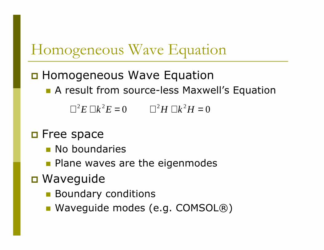
� Homogeneous Wave Equation

� A result from source-less Maxwell’s Equation

� Free space

� No boundaries

� Plane waves are the eigenmodes

� Waveguide

� Boundary conditions

� Waveguide modes (e.g. COMSOL®)

022 =+∇ EkE 022 =+∇ HkH

Free space propagation

� Superposition of all plane waves

� Decompose the plane wave spectrum at z=0

� Add the propagation phase reaching z=z

� Sum all the plane wave components

( ) ( ) ( )∫∫

−−±+=

= βαβα βαβα ddeeEzyxE zkjyxj

z

222

0,,,

z=0z=z

(x,y)

k

kz

Fourier Transform relations

� Superposition of all plane waves

� At z=0

� Decompose the plane wave spectrum

� Spatial function E(x,y) and Spatial Spectrum function E(α,β) is a 2-D Fourier Transform Pair

( ) ( ) ( )∫∫

−−±+=

= βαβα βαβα ddeeEzyxE zkjyxj

z

222

0,,,

( ) ( ) ( )∫∫

+=

== βαβα βα ddeEzyxE yxj

z 0,0,,

( ) ( ) ( )∫∫

+−=

== dxdyezyxEE yxj

z

βα

πβα 0,,

4

1,

20

Use of Fourier Transform Tables

( ) ( ) ( )∫∫

+=

== βαβα βα ddeEzyxE yxj

z 0,0,,

� Be careful where to put 2π

( ) ( ) ( )∫∫

+−=

== dxdyezyxEE yxj

z

βα

πβα 0,,

4

1,

20

Limit of Imaging Resolution

� Visible part of spectrum

� Propagation modes, will reach the image plane

� Evanescent waves

� Will not reach the image plane

� Limit of Imaging Resolution� The finest detail that can be observed in an optical

image is limited by the highest spatial frequency in the planewave spectrum

� roughly equal to the wavelength of the light used to produce that image. (Why?)

� If near field evanescent waves is detected, better image resolution can be attained, e.g., Scanning near-field microscopy

0222 >−− βαk zkje222 βα −−±

0222 <−− βαk

Aperture stop

� The Fourier transform of a multiplication is a convolution

( ) ( ) ( )−+ === 0,,,0,, inctrans zyxEyxAzyxE

( ) ( ) ( ) βαβαββααβα ′′′′′−′−= ∫∫ ddEAE ,,, inctrans

• For a single plane wave incident

( ) ( )00inc ,, ββααδβα −−=E

( ) ( ) ( )( )00

00trans

,

,,,

ββαα

βαββααδββααβα

−−=

′′−′−′′−′−= ∫∫A

ddAE

Aperture stop

� A single plane wave incident on an aperture gives rise to an entire spectrum of plane waves, whose spectral contents are determined by the Fourier transform of the aperture function.

� Including both propagating modes and

� Evanescent waves, which are of paramount importance for super-resolution imaging.

( ) ( )00trans ,, ββααβα −−= AE

• For a single plane wave incident

( ) ( )00inc ,, ββααδβα −−=E

Thin Lens with finite size

� A finite size thin lens can be treated as the same size aperture stop followed by an ideal (infinitely large) thin lens.

� Each plane wave spectral component after the aperture stop focuses into a point at the back focal plane. (Why?)

� Where?

For the spectral component E(α,β), where is the focused point after a thin lens of focal length f?

Thin Lens with finite size

� A finite size thin lens can be treated as the same size aperture stop followed by an ideal (infinitely large) thin lens.

� Each plane wave spectral component after the aperture stop focuses into a point at the back focal plane. (Why?)

( ) ( ) 2

00trans ,, ββααεε −−=−− EyxI yx

0αε =f

k x0β

ε=

fk y

Thin Lens Imaging: Plane-Wave Spectrum method

� A source d0 distance away from the thin lens,

( ) ( ) ( ) βαβα βα ddeEyxE yxj +∫∫= ,, objobj

( ) ( ) 0222

,, objinc dkjeEE βαβαβα −−−=

At thin lens,

� Field distribution at the back focal plane

( ) ( ) ( ) 222220 1obj ,,, yxfjkfyfxjkd ee

f

ky

f

kxEfzyxE ++−−−−

==

� Field distribution at the back focal plane

( ) ( ) ( ) 222220 1obj ,,, yxfjkfyfxjkd ee

f

ky

f

kxEfzyxE ++−−−−

==

( ) ( ) ( )

( ) ( )( )22020

222220

2

1,

yxfdf

kfdk

yxfkfyfxkdyx

+−++−≈

++−−−−=φ

� Paraxial approximation

( ) ( ) ( )( )2202

0 2obj ,,,yxfd

f

kj

fdjk eef

ky

f

kxEfzyxE

+−+−

==

Back focal plane field and Paraxial Approximation

Lens Law: Plane-Wave Spectrum method

� Field distribution at the back focal plane

� Lens Law

( ) ( ) ( )( )2202

0 2obj ,,,yxfd

f

kj

fdjk eef

ky

f

kxEfzyxE

+−+−

==

( )( )22022

yxfdf

kj

e+−

is a quadratic phase front, will focus to a point

fd

fL

−=

0

2

away from the back focal plane.

or ( )( ) 20 ffdfdi =−−

which is the lens law. (compare to ).fdd i

111

0

=+

Spectrum at the image plane

� Field distribution at the back focal plane

( ) ( ) ( )( )2202

0 2obj ,,,yxfd

f

kj

fdjk eef

yk

f

xkEfzyxE

′+′−+−

′′==′′

kfd

x

i −′

=′−α

(x’,y’)(x,y)

f di

kfd

y

i −′

=′− β

• each point on the back focal planecorresponds to a specific direction,i.e., spectral content of image plane.

( )fzyxE =′′ ,, give rise to the spectrum of the image plane

Spectrum and field at the image plane

� Spectrum at image plane

( )

′′=′′

f

yk

f

xkEE ,, objβα k

fd

x

i −′

=′−α kfd

y

i −′

=′− β

recall at object plane f

yk

f

xk ′=

′= βα ,

therefore using the magnification factorf

fdM i −−=

′=

′=

ββ

αα

� Field at image plane

( ) ( ) ( )∫∫ ′′′′== ′+′ βαβα βα ddeEdzyxE ii yxj

iii ,,,

( ) ( ) ( )∫∫

+== βαβα βα ddeEM

dzyxE Myxjiii

ii,1

,, obj2

Image of extended objects

( )( ) ( )( ) ( )

i

iyx

d

kjyx

d

kj

i

jkd

ii dka

dkaJaee

d

eAyxPSF

iii

i

ρρπ

π1222

0 24

,222

020

0

+−+−−

=

� Point spread function (for circular lens)

� Field/Image at the image plane z=di

( )( )( ) ( )

( ) ( )00

1200

220

20

20

0

22

,24

, dydxdka

dkaJeyxEae

d

eAyxE

i

iyx

d

kjyx

d

kj

i

jkd

ii

iii

i

∫∫+−+−−

=ρρπ

π

( ) ( )20

20 MyyMxx ii +++=ρfor 0ddM i=

Image of extended objects

( ) ( ) ( ) 000000 ,,, dydxMyyMxxPSFyxOyxI iiii ∫∫ −−=

( )( )( ) ( )

( ) ( )00

1200

220

20

20

0

22

,24

, dydxdka

dkaJeyxEae

d

eAyxE

i

iyx

d

kjyx

d

kj

i

jkd

ii

iii

i

∫∫+−+−−

=ρρπ

π

( ) ( )20

20 MyyMxx ii +++=ρfor 0ddM i=

In general:

is a convolution of object field and the PSF in spatial domain,therefore in plane-wave spectral domain

( ) ( ) ( )βαβαβα ,,, PSFOI =

The Optical Transfer Function (OTF)

� For imaging with incoherent light source, the power PSF is

( ) ( ) 2,, yxPSFyxPPSF =

� Optical Transfer Function (OTF) is the Fourier transform of PPSF

( ) ( ) 2, .., yxPSFTFOTF =βα

for ( ) ( ) ( )∫∫

+= βαβα βα ddeyxPSFPSF yxj,,

( ) ( ) ( ) βαβαββααβα ′′′′′+′+= ∫∫ ddPSFPSFOTF ,,, *

is the complex autocorrelation of spectral domain PSF. (Why?)

The Modulation Transfer Function (MTF)

� MTF is the magnitude of OTF

( ) ( )βαβα ,, OTFMTF =

� Example: MTF of an ideal lens

( )yxA , ( ) ( )βαβα ,, PSFA =

Example: MTF of an ideal lens

( ) ( ) ( ) βαβαββααβα ′′′′′+′+= ∫∫ ddPSFPSFOTF ,,, *

( ) ( )

∆−∆−∆=

∆−∆−∆=

∆−==∆

−−2

122

12

222shaded

1cos2

1cos2

sin222

aaaa

aa

aa

aaaaAMTF

ππ

πφφπ

Example: MTF of an ideal lens

� Another way to calculate

( )( ) ( )( ) ( )

i

iyx

d

kjyx

d

kj

i

jkd

ii dka

dkaJaee

d

eAyxPSF

iii

i

ρρπ

π1222

0 24

,222

020

0

+−+−−

=

( ) ( ) ( )( )2

2122

2

022

4,

i

i

iii

dka

dkaJa

d

AyxPSF

ρρπ

π=

( ) ( ) ( )( )

( )yxj

i

i

i

edka

dkaJdda

d

AOTF βα

ρρϕρρπ

πβα +−

∫∫= 2

2122

2

0 24

,

( ) ( )( ) ( )∫∝ θρ

ρρρβα sin, 0

21 kJ

dka

dkaJdOTF

i

i

Example: MTF of an ideal lens

( ) ( )( ) ( ) ρθρ

ρρβα dkJ

dka

dkaJOTF

i

i∫∝ sin, 0

21

Example: MTF of an ideal lens

( ) ( )( ) ( ) ρθρ

ρρβα dkJ

dka

dkaJOTF

i

i∫∝ sin, 0

21

Measuring the MTF

� MTF can be measured experimentally

� Shearing interferometer measurement of MTF

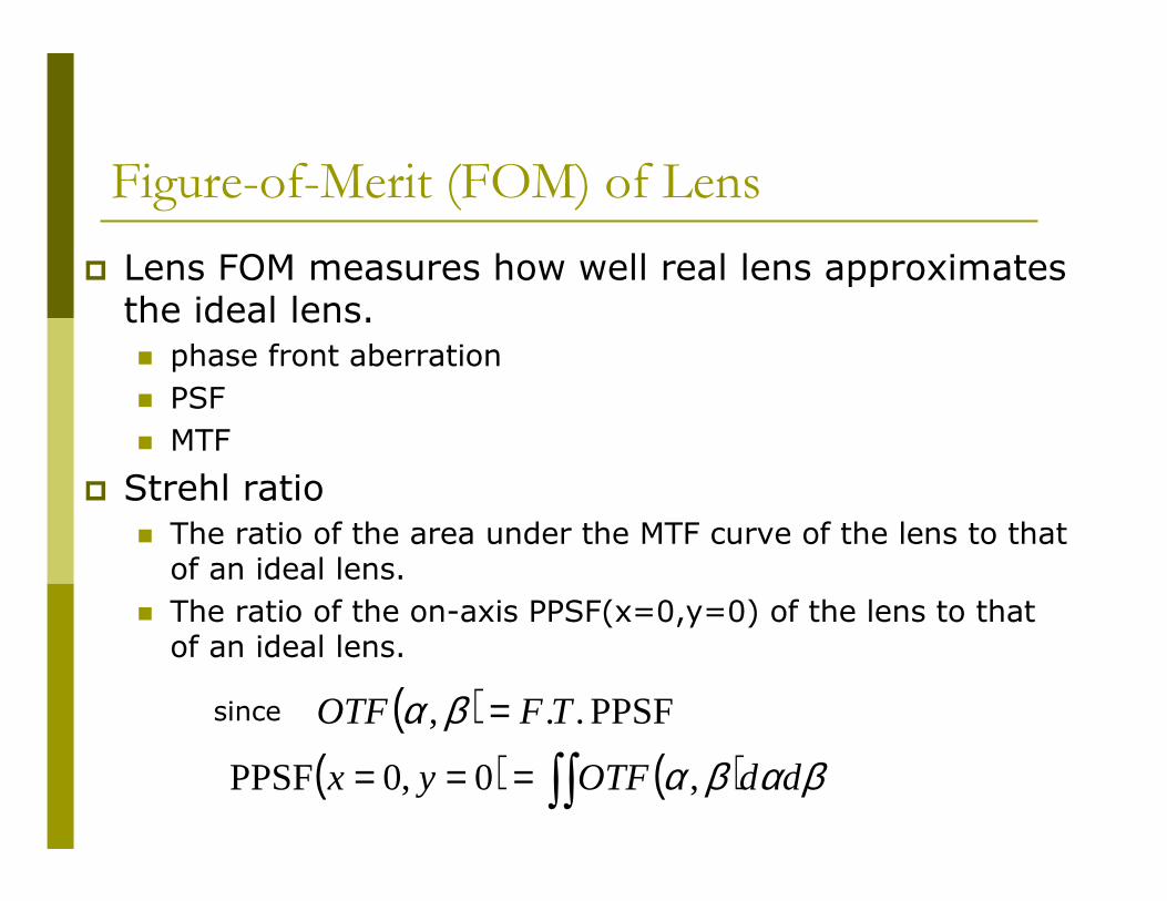
Figure-of-Merit (FOM) of Lens

� Lens FOM measures how well real lens approximates the ideal lens.

� phase front aberration

� PSF

� MTF

� Strehl ratio

� The ratio of the area under the MTF curve of the lens to that of an ideal lens.

� The ratio of the on-axis PPSF(x=0,y=0) of the lens to that of an ideal lens.

( ) PPSF .., TFOTF =βαsince

( ) ( ) βαβα ddOTFyx ∫∫=== ,0,0PPSF