Leonid E. Zhukov - Leonid Zhukov · Lecture outline 1 Epidemic models SI model SIS model SIR model...

Epidemics

Leonid E. Zhukov

School of Data Analysis and Artificial IntelligenceDepartment of Computer Science

National Research University Higher School of Economics

Structural Analysis and Visualization of Networks

Leonid E. Zhukov (HSE) Lecture 12 07.04.2015 1 / 24

Lecture outline

1 Epidemic modelsSI modelSIS modelSIR model

2 Branching processGalton-Watson process


Epidemic dynamics models

Mathematical epidimiology

W. O. Kermack and A. G. McKendrick, 1927

Deterministic compartamental model (population classes) {S , I ,T}S(t) - succeptable, number of individuals not yet infected with thedisease at time t

I (t) - infected, number of individuals who have been infected with thedisease and are capable of spreading the disease.

R(t) - recoverd, number of individuals who have been infected andthen recovered from the disease, can’t be infected again or totransmit the infection to others.

Fully-mixing model

Closed population (no birth, death, migration)

Models: SI, SIS, SIR, SIRS,..


SI model

S(t) -susceptible , I (t) - infected

S −→ I

S(t) + I (t) = N

β - infection/contact rate, number of contacts per unit time

Infection equation:

I (t + δt) = I (t) + βS(t)

NI (t)δt

dI (t)

dt= β

S(t)

NI (t)


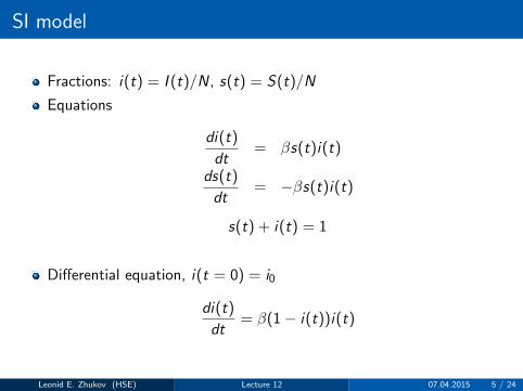
SI model

Fractions: i(t) = I (t)/N, s(t) = S(t)/N

Equations

di(t)

dt= βs(t)i(t)

ds(t)

dt= −βs(t)i(t)

s(t) + i(t) = 1

Differential equation, i(t = 0) = i0

di(t)

dt= β(1− i(t))i(t)


Logistic growth function

Solution:

i(t) =i0

i0 + (1− i0)e−βt

Limit t →∞

i(t)→ 1

s(t)→ 0

in image i0 = 0.05, β = 0.8


SIS model

S(t) -susceptable , I (t) - infected,

S −→ I −→ S

S(t) + I (t) = N

β - infection rate (on contact), γ - recovery rate

Infection equations:

ds

dt= −βsi + γi

di

dt= βsi − γi

s + i = 1

Differential equation, i(t = 0) = i0

di

dt= (β − γ − i)i


SIS model

Solution

i(t) = (1− γ

β)

C

C + e−(β−γ)t

where

C =βi0

β − γ − βi0

Limit t →∞

β > γ , i(t)→ (1− γ

β)

β < γ , i(t) = i0e(β−γ)t → 0


Logistic function

β > γ, i(t)→ (1− γβ )

β < γ, i(t) = i0e(β−γ)t → 0


SIR model

S(t) -susceptable , I (t) - infected, R(t) - recovered

S −→ I −→ R

S(t) + I (t) + R(t) = N

β - infection rate, γ - recovery rate

Infection equation:

ds

dt= −βsi

di

dt= βsi − γi

dr

dt= γi

s + i + r = 1


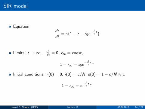
SIR model

Equationds

dt= −βs dr

dt

1

γ

s = s0e−βγr

dr

dt= γ(1− r − s0e

−βγr )

Solution

t =1

γ

∫ r

0

dr

1− r − s0e−βγr


SIR model

βγ = 4

i0 = 0.1


SIR model

βγ = 0.5

i0 = 0.1


SIR model

Equationdr

dt= γ(1− r − s0e

−βγr )

Limits: t →∞, drdt = 0, r∞ = const,

1− r∞ = s0e−βγr∞

Initial conditions: r(0) = 0, i(0) = c/N, s(0) = 1− c/N ≈ 1

1− r∞ = e−βγr∞


SIR model

r∞ = 1− e−R0r∞ , R0 =β

γ

(r∞)′|r∞=0 = (1− e−R0r∞)′|r∞=0,

critical point: R0 = 1


SIR model

r∞ - the total size of the outbreak

Epidemic threshold

Epidemics: R0 > 1, β > γ , r∞ = const > 0

No epidemics: R0 < 1, β < γ , r∞ → 0

Basic reproduction number

R0 =β

γ

It is average number of people infected by a person before his recovery

R0 = E [βτ ] = β

∫ ∞0

γτe−γτdτ =β

γ


Model of contagion

Simple model of contagion (decease transmission)

1st-wave: first infected person enters the population and transmits toeach person he meets with probability p. Suppose he meets k peoplewhile contagious

2nd-wave: Each infected person from 1st wave meets k new peopleand independently transmits infection with probability p

3rd-wave: ....

This is Galton-Watson branching stochastic process (Proposed by FrancisGalton 1889 as a model for extinction of family names)


Branching process

image from David Easley, Jon Kleinberg, 2010


Branching process

Random branching process:

let ξni - number of transmitted infections by ith node on level n

let Zn - number of infected on level n, Z0 = 1. Then:

Zn+1 =Zn∑i=1

ξ(n)i

If each node has k neighbors, transmits infection with probability p,Average number of infected people E [ξni ] = pk = R0 - basicreproductive number

Recursion

E [Zn+1] = E [Zn∑i=1

ξ(n)i ] = E [ξ

(n)i ] E [Zn] = pk E [Zn]

E [Zn] = (pk)n = Rn0


Branching process

Galton-Watson branching random process:

if R0 = 1, the mean of number of infected nodes does not change

if R0 > 1, the mean grows geometrically as Rn0

if R0 < 1, the mean shrinks geometrically as Rn0

R0 = 1 - point of phase transition


Branching process

Extinction probability

let qn - probability that infection persists n steps (levels of the tree)

pqn−1 - probability that spreads through one first contact and thensurvives n − 1 levels

(1− pqn−1)k - probability that will not spread through any of thesubtries

(1− pqn−1)k = 1− qn


Branching process

Recurrence (qn - probability that infection persists through n steps)

qn = 1− (1− pqn−1)k


Branching process

limiting probability q∗ = limn→∞ qn

q∗ = 1− (1− pq∗)k

Slope:pk(1− pq)k−1

∣∣q=0

= 1

When R0 = pk > 1, there is a non zero probability of infection persists


References

A Contribution to the Mathematical Theory of Epidemics. , Kermack,W. O. and McKendrick, A. G. , Proc. Roy. Soc. Lond. A 115,700-721, 1927.

The Mathematics of Infectious Disease, Herbert W. Hethcote, SIAMReview, Vol. 42, No. 4, p. 599-653, 2000


Date post:	31-May-2020
Category:	Documents
Upload:	others
View:	12 times
Download:	2 times

Leonid E. Zhukov - Leonid Zhukov · Lecture outline 1 Epidemic models SI model SIS model SIR model...

Documents