M: I'm excited to tell you about neural networks today. You may be familiar with neural networks because you have one, in your head.C: I do?M: Well, yeah. I mean, you have a network neurons. Like, you know neurons, like brain cells. Let me, I'll draw you one.C: Okay.M: So this is my template drawing, a nerve cell, a neuron. You've got billions and billions of these inside your head. And most of them have a pretty similar structure, the main part of the cell called the cell body. And then there's this thing called an axon which kind of is like a wire going forward to a set of synapses which are kind of little gaps between this neuron and some other neuron. And what happens is, information spike trainsC: Woo woo!M: Travel down the axon. When the cell body fires it has an electrical impulse it travels down the, the axon and then causes across the synapses excitation to occur on other neurons which themselves can fire. Again by sending out spike trains. And so they're very much a kind of a computational unit and they're very, very complicated. To a first approximation, as is often true with first approximations they're very simple. Sort of by definition of first approximation. So what, in the field of artificial neural networks we have kind of a cartoonish version of the neuron and networks of neurons and we actually put them together to compute various things. And one of the nice things about the way that they're set up is that they can be tuned or changed so that they fire under different conditions and therefore compute different things. And they can be trained through a learning process. So that's what we're going to talk through if you haven't heard about this before.C: Okay.
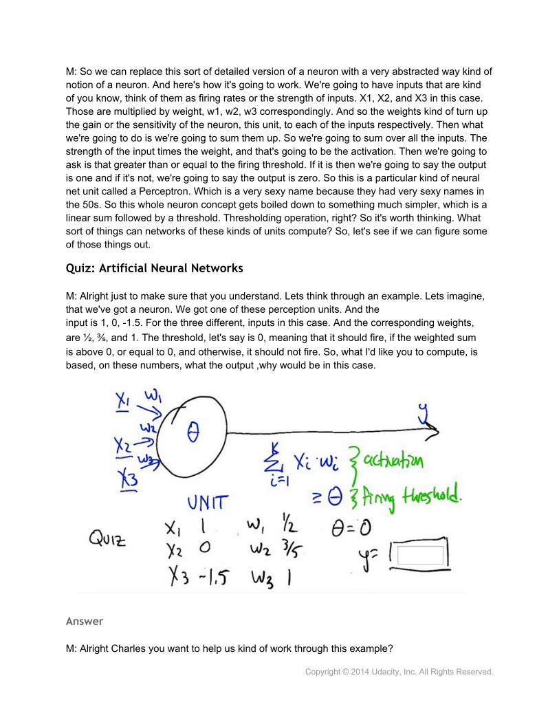
M: So we can replace this sort of detailed version of a neuron with a very abstracted way kind of notion of a neuron. And here's how it's going to work. We're going to have inputs that are kind of you know, think of them as firing rates or the strength of inputs. X1, X2, and X3 in this case. Those are multiplied by weight, w1, w2, w3 correspondingly. And so the weights kind of turn up the gain or the sensitivity of the neuron, this unit, to each of the inputs respectively. Then what we're going to do is we're going to sum them up. So we're going to sum over all the inputs. The strength of the input times the weight, and that's going to be the activation. Then we're going to ask is that greater than or equal to the firing threshold. If it is then we're going to say the output is one and if it's not, we're going to say the output is zero. So this is a particular kind of neural net unit called a Perceptron. Which is a very sexy name because they had very sexy names in the 50s. So this whole neuron concept gets boiled down to something much simpler, which is a linear sum followed by a threshold. Thresholding operation, right? So it's worth thinking. What sort of things can networks of these kinds of units compute? So, let's see if we can figure some of those things out.
Quiz: Artificial Neural Networks
M: Alright just to make sure that you understand. Lets think through an example. Lets imagine, that we've got a neuron. We got one of these perception units. And theinput is 1, 0, -1.5. For the three different, inputs in this case. And the corresponding weights, are ½, ⅗, and 1. The threshold, let's say is 0, meaning that it should fire, if the weighted sum is above 0, or equal to 0, and otherwise, it should not fire. So, what I'd like you to compute, is based, on these numbers, what the output ,why would be in this case.
Answer
M: Alright Charles you want to help us kind of work through this example?
C: Sure. So ,we multiply x1 times w1 so that gives us a 1/2M: Um-huh.C: We multiply 0 times 3/5 which would get a 0 and we multiply -1.5 times 1. Which will give us -3/2. And so, the answers negative. Whatever it is.M: It is right, so it's, this was negative ahead, -1.5 plus a 1/2, so it should be negative one.C: Right.M: And, but that's not the output that we should actually produce, right? That's the activation. What do we do with the activation?C: Well we see if the activation is above our threshold fata, which in this case is 0, and it is not So the output should be 0.M: Good.
How Powerful is a Perceptron Unit
M: Alright. Well we'd like to try to get an understanding of how powerful one of these perceptron units are. So, what is it that they actually do? So they, they return, in this case either 0 or 1as a function of a bunch of inputs. So let's just for simplicity of visualization, let's just imagine that we've got 2 inputs, X1 and X2. So Charles, how could we represent the region in this input space that is going to get an output of 0 versus the region that's going to get an output of 1.C: Order the weights.M: Right. So indeed, the weights matter. So let's, let's give some concrete values to these weights. And let's just say, just making these up that weight 1 is a half, weight 2 is a half, and our threshold data is three quarters. So now what we want to do is again, break up this space into where's it going to return 1 and where's it going to return 0.C: Okay, so I think I know how to figure this out. So there's 2 sort of extreme examples, so let's take a case where X1 is 0.M: X1 is 0. Okay, good. So that's this Y axis.C: Alright. So if X1 is 0, what value would X2 have to be in order to break a threshold of three quarters? Well, the weight on X2 is a half.M: Mm-hm.C: So then, the value of X2 would have to be twice as much as the threshold which in this case is 1.5.M: Right. So we're trying to figure out where is it, if X1 is 0, where does X2 need to be so that we're exactly at the threshold. So that's going to be.C: Right.M: The X2 times the weight, which is half has to exactly equal the threshold which is three quarters. So, if we just solve that out, you get X2 equals a dividing line. So anywhere above here, what's it going to return?C: It will return, it will break the threshold, and so it will return a 1.M: These are all going to be 1s and then below this these are all going to be 0s.C: Right.M: Alright. Well now we have a very, very skinny version of the picture. Well what else can we do?
C: Well we can do the same thing that we just did except we can swap X2 and X1 because, they have the same weight. So, we could say X2 equal to 0 and figure out what the value of X1 has to be.M: Good, and that seems like it would be exactly the same algebra, and so we get X1 is 3 halves, gives us at the one and a half point above here are going to be 1s and below here are going to be 0s. Okay, so now we've got 2 very narrow windows, but what we notice is that the relationships are all linear here. So solving this linear inequality gets us a picture like this. So this perceptron computes a kind of half plane right? So, so the half of the plane that's above this line, the half plane that's above this line is getting us the 1 answers and below that line is giving us a zero answers.C: So Michael can we generalize from this, so you're telling me that because of the linear relationship drawn out by a perceptron that perceptrons are always going to compute lines.M: Yeah. Always going to compute, yeah these half planes right. So there's a dividingline where you're equal to the threshold and that's always going to be a linear function and then it's going to be you know, to the right of it or to the left of it, above it or below it but its always halves at that point.C: Okay, so perception is a linear function, and it computes hyperplanes.M: Yeah, which maybe in some sense it doesn't seem that interesting, but it turns out we're already in a position to compute something fascinating. So let's do a quiz.
Quiz: How Powerful is a Perceptron Unit
M: So this example that we, you know, created just at random actually is it computes an interesting function. So let's, let's focus on just the case where our X1 is in the set zero, one and X2 is in the set zero, one. So those are the only inputs that we care about, combinations of those. What is Y computing here? What is the name of that relationship that function that's being computed? And so, just as a hint, there's a nice short one-word answer to this if you can kind of plug it through and see what it is that it's computing.
M: Charles, can you figure this out?C: Yes, I believe I can. So, the first thing to note is that because we're sticking with just 0 and 1, and not all possible values in between, we're thinking about a binary function. And the output is also binary. Which makes me think of Boolean functions, where zero represents false and one represents true, which is a common trick in machine learning.M: Alright, so and let me, let me mark those on the picture here. So we're talking about the only four combinations are here. And you're saying in particular. That we're interpreting these as combinations of true and false.C: RightM: False, false, true, false, false, true, and true, true.C: Exactly and if you look at it the only way that you get something above the line is when both are true.M: Also take conjunction. You know we're setting these numerical values but it actually has gives us a way of specifying a kind of logic key.C: Right. So here's a question for you Michael. Could we do OR?M: That's a very good question. OR looks a lot like AND in this space, it, it seems like it ought to be possible. So let's let's do that as a quiz.
Quiz: How Powerful is a Perceptron Unit OR
M: Alright, so we're going to go in the opposite direction now. And we're saying, we're going to tell you what we want y to be, we want y to be the OR function. So it should be outputtinga one if either x one or x two is one, and otherwise it should output a zero. And what you need to do is fill in numbers for weight one, weight two, and theta so that it has that semantics. Now, just so you know, there is no unique answer here. There's a whole bunch of answers that will work, but we're going to check to see that you've actually typed in one that, that works.
M: Alright Charles, let's, let's figure this one out. It turns out, as I said, there's lots of different ways to make this work, but, what we're going to do is move that line that we had for conjunction. If we, what we really want to do now is figure out how to move it down so that these three points are in the green zone. They're going to output 1 because they're the only one that's left in the zero zone in the red zone is the zero, zero case.C: Right.M: So, How are we going to be able to do that?C: Well, since we want it to be case that either X2 or X1, being one get you above the line, then, we need a threshold and a set of weight that put either one of them over. You don't have to have both of them. You only need one of them.M: Okay.C: So, let's imagine a case where X1 is one and X2 is 0. Oh, you're right. There's a whole lot of answers, so a weight of 1, for X1, would give you a 1. Right?M: YesC: And so, if we made the threshold 1, that would work.M: What about weight 2?C: Well, we do exactly the same thing. So, we set weight 2 equal to 1. That means that in the case where both of them are 0, you get 0 plus 0, which gives you something less than 1. If one of them is 1 and the other is 0, you get 1, which gives you right at the threshold. If both of them are one then you get two, which is still greater than one.M: Good, alright, that seems like it worked. The other way we could do it is keeping the weights where they were before, that just moves this line nice and smoothly down. Right? So before, we had a, a threshold one and a half. Now we need a threshold of a half. That ought to do it.C: Yep.M: Or even less, as long as it's greater than zero. So, a quarter should work, as well.Can we do NOT?C: What's NOT of two variables?M: That's a good question. Let's do NOT of one variable.C: Okay.
Quiz: How Powerful is a Perceptron Unit NOT
M: Maybe you should help me finish this picture here. So what we've got is X1 is our variableand so we can take on any sort of values. And I marked -1, 0, and 1 here. And if we're doing NOT then what should the output be for each of these different values of X1? So if X1 is 0, then we want the output to be 1. And if X1 is 1, we want the output to be 0. Alright, so now what we'd like you to do is say okay, what should weigh 1 and what should theta be so that we get this kind of NOT behavior.
M: Alright Charles, you were about to say, how we could do this.C: We need to flip 0 and 1, which suggests that either our weight or our threshold needs to be negative. The threshold is above, it's going to end up being our weight being negative. If we have a 0, we want to turn that into something above the threshold and if it's a one, we want it to be below the threshold. So, why don't we make the weight negative one.M: Okay.C: And that turns a 0 into a 0 and it will turn a 1 into a -1. Alright.M: And so, then the threshold just has to be 0.C: So that would mean that anything, I see, so anything that's negative will be greater than, zero or negative would be greater than or equal to the threshold. And anything on the otherside of that. would be under the threshold. So we get this kind of dividing line at one, so were taking advantage of the fact the equation had a greater than or equal to in it. So, yeah,right, that ought to be a NOT. So we've got AND, OR and NOT that are all expressible as perceptron units.M: Hey that's great because if we have AND, OR, and NOT, then we can represent any Boolean function.C: Well, do we know that? We know that if we combine them together, we combine these perceptron units together can we express any perceptron, or sorry, any boolean function that we want using a single perception?M: What do we normally do in this case? What's the most evil function we can think of?C: Yes indeed. We'll when we're working on decision trees, the thing that was so evil was the XOR parity more generally.M: Right.C: So, alright. Maybe if we can do that, we can do anything. So, let's, let's give it a shot.
Quiz: XOR as Perceptron Network
M: Alright so here's what we're going to do. We're going to try to figure out how to compute XOR. Instead of a single perceptron, which we know is impossible, we can do it as a
network of perceptron. To make it easier for you, here's how we're going to set it up. We've got x1 and x2 as our inputs We've got two units. This first unit is just going to compute and add and we already know how to do that. We've already figured out what weights need here. And what the threshold needs to be, so that the output will be the AND of those two inputs. So, that's all good. It turns out the second unit, with three inputs, X1, X2, and the AND of X1 and X2 we can use to set the weights on that so that the output is going to be XOR. So, what we'd like you to do is, figure out how to do that. How do you set this weight - Is the input of X1, this way which is the and input, and this way which is the X2 input, and the threshold. So that it's going to actually compute an XOR. And, and just so you know, this is not a trick question. You really can do it this time.
Answer
M: So, okay, so, how we, how we going to solve this?C: Okay, so, I guess the first thing to do is if you look at the table you have at the bottom, it tells us what the truth tables are for AND and XOR, alright? So, we know that Boolean functions, can all be represented as combinations of AND, OR, and NOT. So, I'm going to recommend you feel out that empty column with OR.
M: So, OR is like that.C: Right. And you'll notice, if you look at AND, OR and XOR. OR looks just like XOR except at the very last row.M: In the second, okay good, uh-huh, and in that row.C: Right, and, AND on the other hand, tells us a one only on the last row. So what, I'm going to suggest that we really want that last node to do in your drawing, is to compute the or of X1 or X2. And produce the right answer, except in the case of the last row, which we only want to turn off when and happens to be true. So really what that node is computing OR minus AND.M: Alright, so how do we make this OR minus AND? So the way we did OR before well we did it a couple of different ways. But one is we gave weights of one on the two inputs. And then a threshold of one. And that made, ignoring everything else at the moment, this unit will now turn on if either x1 or x2 are on. And otherwise it will stay off.C: Right. So what's the worst case? The lowest value that you can get. Is when one of those is one and one of those is zero, which means that the sum into those will be, in fact, one.M: Yeah.C: Right? So, if the AND comes out as being true, it's going to give us some positive value. So, if we just simply have a negative wait there, that will subtract out. Exactly in the case ,when AND is on. It's not going to quite give us the answer we want, but it's a good place to start to think about it.M: Alright, so like just a negative weight, like negative one.C: Mm-hmm.M: Alright. So does that work?C: Not quite.M: Alright, and why doesn't it work? Because well certainly when AND is off then we really are just getting the OR, that's all good.C: Yeah.M: But if both x1 and x2 are both on, then the sum here is going to be two minus the one that we get from the AND which is still one.C: So, minus one isn't enough?M: Minus with both, maybe we can do more than that. Maybe we can do minus two. What happens if we do minus two? Then we've got X1 and X2 if they're both on. Then we get a sum of one minus two plus one or zero. Which is less than our threshold so it will output zero. And in the other two cases, right, when AND is off then it just acts like OR. So this actually kind of does the right thing. Its actually OR minus kind of AND times two. [LAUGH]C: Right. And there you go. And of course there's an infinite number of solutions to this.
Perceptron Training
M: Alright. So in the examples up to this point, we've be setting the weights by hand to make various functions happen. And that's not really that useful in the context of machine learning. We'd really like a system that given examples, finds weights that map the inputs to the outputs. And we're going to actually look at two different rules that have been developed for doing exactly that, to figuring out what the weights ought to be from training examples. One is called
the the Perceptron Rule, and the other is called gradient descent or the Delta Rule. And the difference between them is the perception rule is going to make use of the threshold outputs, and the, the other mechanism is going to use unthreshold values. Alright so what we need to talk about now is the perception rule for how to set the weights of a single unit. So that it matches some training set. So we've got a training set, which is a bunch of examples of x. These are vectors and we have y's which are zeros and ones which are the, the output that we want to hit. And what we want to do is set the, set the weights so that we capture this, this same data set. And we're going to do that by, modifying the weights over time.C: Oh, Michael, what's the series of dashes over on the left.M: Oh, sorry, right. I should mention that, so one of the things that we're going to do here iswere going to give a learning rate for the weights W, and not give a learning rule for Theta But we do need to learn the theta. So there's a, there's a very convenient trick for actually learning them by just treating it as another kind of weight. So if you think about the way that the thresholding function works. We're taking a linear combination of the W's and X's, then we're comparing it to theta. But if you think about just subtracting theta from both sides, then, in some sense theta just becomes another one of the weights, and we're just comparing to zero. So what, what I did here was take the actual data, the x's, and I added what is sometimes called a bias unit. So basically the input is one always to that. And the weight corresponding to it is going to correspond to negative theta ultimately. This just simplifies things so that the threshold can be treated the same as the weights. So from now on, we don't have to worry about the threshold. It just gets folded into the weights, and all our comparisons are going to be just to zero instead of theta. Centric, yeah. It certainly makes the math shorter. So okay, so this is what we're going to do. We're going to iterate over this training set, grabbing an x, which includes the bias piece, and the y. Where y is our target X is our input. And what we're going to do is we're going to change weight i, the weight corresponding to the ith unit, by the amount that we're changing the weight by. So this is sort of a tautology, right. This is truly just saying the amount we've changed the weight by is exactly delta W - in other words the amount we've changed the weight by. So we need to define that what that weight change is. The weight change is going to be find as falls. We're going to take the target, the thing that we want the output to be. And compare it to, what the network with the current weight actually spits out. So we compute this, this y hat. This approximate output y. By again summing up the inputs according to the weights and comparing it to zero. That gets us a zero one value.So we're now comparing that to what the actual value is. So what's going to happen here, if they are both zero so let's, let's look at this. Each of y and y that can only be zero and one. If they are both zeros then this y minus y hat is zero. If they're both ones and what does that mean? It means the output should have been zero and the output of our current. Network really was zero, so that's, that's kind of good. If they are both ones, it means the output was supposed to be one and our network outputted one, and the difference between them is going to be zero. But in this other case, y minus y hat, if the output was supposed to be zero, but we said one, our network says one, then we get a negative one. If the output was supposed to be one and we said zero, then we get a positive one. Okay, so those are the four cases for what's happening here. We're going to take that value multiply it by the current input to that unit i, scale it down by the sort of thing that is going to be cut the learning rate and use that as the the weight update change. So essentially what we are saying is if the output is already correct either both on or both off. Then there's going to
be no change to the weights. But, if our output is wrong. Let's saythat we are giving a one when we should have been giving a zero. That means the total here is too large. And so we need to make it smaller. How are we going to make it smaller? Which ever input XI's correspond to, very large values, we're going to move those weights very far ina negative direction. We're taking this negative one times that value times this, this little learning rate. Alright, the other case is if the output was supposed to one but we're outputting a zero, that means our total is too small. And what this rule says is increase the weights essentially to try to make the sum bigger. Now, we don't want to kind of overdo it, and that's what this learning rate is about. Learning rate basically says we'll figure out the direction that we want to move things and just take a little step in that direction. We'll keep repeating over all of the input output pairs. So, we'll have a chance to get into really building things up, but we're going to do it a little bit at a time so we don't overshoot. And that's the rule. It's actually extremely simple. Like, you,actually writing this in code is, is quite trivial. And and yet, it does some remarkable things. So let's imagine for a second that we have a training set that looks like this. It's in two dimensions, again, so that it's easy to visualize. That we've got. A bunch of positive examples, these green x's and we've got a bunch of negative examples these red x's, and were trying to learn basically a half plane right? Were trying to learn a half plane that separates the positive from the negative examples. So Charles do you see a, half plane that we could put in here that would do the trick?C: I do.M: What would it look like?C: It's that one.M: By that one do you mean, this one?C: Yeah. That's exactly what I was thinking, Michael.M: That's awesome! Yeah, there are isn't a whole lot of flexibility in what the answer is in this case, if we really want to get all greens on one side and all the reds on the other. If there is such a half plane that separates the positive from the negative examples, then we say that the data set is linearly separable, right? That there is a way of separating the positives and negatives with a line. And what's cool about the perception rule, is that if we have data that is linearly separable. The Perceptron Rule will find it. It only needs a finite number of iterations to find it. In fact, which I guess is really the same as saying that it will actually find it. It won'teventually get around to getting to something close to it. It will actually find a line, and it will stopsaying okay I now have a set of weights that, that do the trick. So that's happens if the data set is in fact linearly separable and that's pretty cool. It's pretty amazing that it can do that, it's a very simple rule and it just goes through and iterates and, and solves the problem. So. Charles Sened solves the problem. So.C: I can think of one. What if it is not linearly separable?M: Hmm, I see. So, if the data is linearlly separable, then the algorithm works, so the algorithm simply needs to only be run when the data is linearlly separable. It's generally not that easy tell actually, when your data is linearly separable especially, here we have it in two dimensions, if it's in 50 dimensions, know whether or not there is a setting of those perimeters that makes it linearly separable, not so clear.C: Well there is one way you could do it.M: Whats that?
C: You could run this algorithm, and see if it ever stops. I see, yes of course, there's a problem with that particular scheme, right, which says, well for one thing this algorithm never stops, so wait, we need to, we need to address that. But, but really we should be running this loop here, while, there's some error so I neglected to say that before. But what you'll notice is if you continue to run this after the point where it's getting all the answers right. It found a set of weights that lineally separate the positive and negative instances what will happen is when it gets to this delta w line that y minus y hat will always be zero the weights will never change we'll go back and update them by adding zero to them repeatedly over and over again. So. If it ever does reach zero error, if it ever does separate the data set then we can just put a little condition inthere and tell it to stop filtering So what you are suggesting is that we could run this algorithm and if it stops then we know that it is linearly separable and if it doesn't stop Then we know that it's not linearly separable, right? By this guarantee.M: Sure.C: The problem is we, we don't know when finite is done, right? If, if this were like 1,000 iterations, we could run it for 1,000 if it wasn't done. It's not done, but all we know at this point is that it's a finite number of iterations, and so that could be a thousand, 10 thousand, a million, ten million, we don't know, so we never know when to stop and declare the data set not linearly separable.M: Hmm, so if we could do that, then we would have solved the halting problem, and we would all have nobel prizes Well, that's not necessarily the case. But it's certainly the other direction is true. That if we could solve the halting problem, then we could solve this.C: Hm.M: But it could be that this problem might be solvable even without solving the halting problem.C: Fair enough. Okay.
Gradient Descent
M: So we are going to need a learning algorithm that is more robust to non-linear separability or linear non-separability. Does that sound right?C: Non-linear separabilityM: Non?C: Yeah think of it. Left parenthesis, linear sep, spreadability left parenthesis.M: There we go, that's right, negating the whole phrase, very good. So Gradient descent is going to give us an algorithm for doing exactly that. So, what we're going to do now is think of things this way. So what we did before was we did a summation over all the different input features of the activation on that input feature times the weight, w, for that input feature. And we sum all those up and we get an activation. And then we have our estimated output as whether or not that activation is greater than or equal to zero. So let's imagine that the output is not thresholded when we're doing the training, and what we're going to do instead is try to figure out the weight so that the non thresholded value is, as close to the target as we can. So this actually kind of brings us back to the regression story. We can define an error metric on the
weight vector w. And the form of that's going to be one half, times the sum over all the data in the dataset, of what the target was supposed to be for that particular example. Minus what the activation actually was. Right? The activation being the dot product between the weights and the input and we're going to square that. We're going to square that error and we want to try to now minimize that. C: Hey Michael, can I ask you a question?M: Sure.C: Why one half of that?M: Mm. Yes. It turns out that it turn, in terms of minimizing the error this is just a constant and it doesn't matter. So why do we stick in a half there? Let's get back to that.C: Okay.M: Just like in the regression case we're going to fall back to calculus. Right, calculus is going totell us how we can push around these weights, to try to push this error down. Right, so we would like to know. How does changing the weight change the error, and lets push the weight in the direction that causes the error to go down. So we're going to take the partial derivative of the, this aerometric with respect to each of the individual weights, so that we'll know for each weight which way we should push it a little bit to move in the direction of the gradient. So that's the partial derivative with respect to weight wi, of exactly this error measure. So to take this partial derivative we just use the chain rule as we always do. And what is it to take the derivative of something like this, if you have this quantity here. We take the power, move it to the front, keep this thing, and then take the derivative of this thing. So this now answers your question, Charles. Why do we put a half in there? Because down the line, it's going to be really convenient that two and the half canceled out. So, it's just going to mean that our partial derivative is going to look simpler, even though our error measure looked a little bit more complicated. So what we're left with then, is exactly what I said,the sum over all these data points of what was inside this. Quantity here times the derivative ofthat, and here I expanded the a to be, the definition of the a. Now, we need to take the partial derivative with respect to weight w i of this sum that involves a bunch of the ws in it. So, when don't match the w i, that derivative is going to be zero because changing the weight won't have any impact on it. The only place where this changing this weight has any impact is at x of i. So that's what we end up carrying down. This summation disappears. And all that's left is just the one term that matches the weight that we care about. So this iswhat we're left with. Now the derivative of the error with respect to any weight w sub i. Is exactly this sum. The sum of the difference between the activation and the target output times the activation on that input unitC: You know? That looks exactly like, almost exactly like the rule that we use with the perceptrons before.M: It does indeed! What's the difference? Well, actually let's Let's write this down. This is now just a derivative, but let's actually write down what our weight update is going to be because we're going to take a little step in the direction of this derivative and it's going to involve a learning rate.
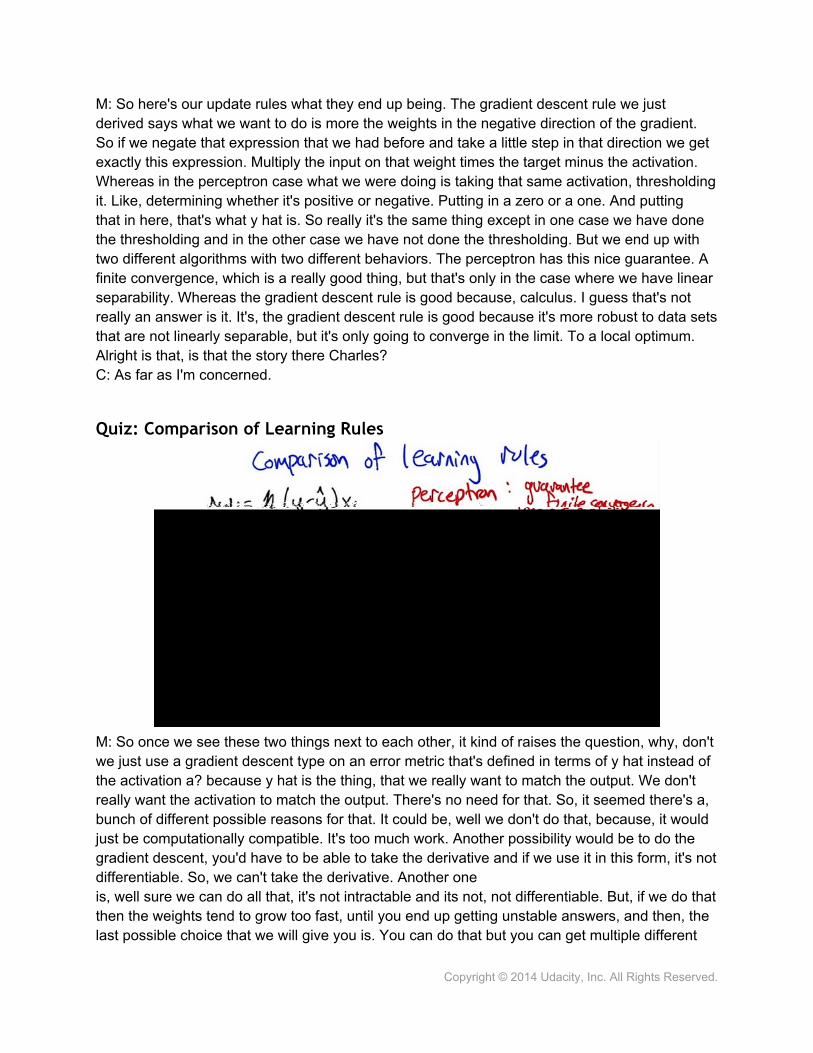
M: So here's our update rules what they end up being. The gradient descent rule we just derived says what we want to do is more the weights in the negative direction of the gradient. So if we negate that expression that we had before and take a little step in that direction we get exactly this expression. Multiply the input on that weight times the target minus the activation. Whereas in the perceptron case what we were doing is taking that same activation, thresholding it. Like, determining whether it's positive or negative. Putting in a zero or a one. And putting that in here, that's what y hat is. So really it's the same thing except in one case we have done the thresholding and in the other case we have not done the thresholding. But we end up with two different algorithms with two different behaviors. The perceptron has this nice guarantee. A finite convergence, which is a really good thing, but that's only in the case where we have linear separability. Whereas the gradient descent rule is good because, calculus. I guess that's not really an answer is it. It's, the gradient descent rule is good because it's more robust to data sets that are not linearly separable, but it's only going to converge in the limit. To a local optimum. Alright is that, is that the story there Charles?C: As far as I'm concerned.
Quiz: Comparison of Learning Rules
M: So once we see these two things next to each other, it kind of raises the question, why, don't we just use a gradient descent type on an error metric that's defined in terms of y hat instead of the activation a? because y hat is the thing, that we really want to match the output. We don't really want the activation to match the output. There's no need for that. So, it seemed there's a, bunch of different possible reasons for that. It could be, well we don't do that, because, it would just be computationally compatible. It's too much work. Another possibility would be to do the gradient descent, you'd have to be able to take the derivative and if we use it in this form, it's not differentiable. So, we can't take the derivative. Another oneis, well sure we can do all that, it's not intractable and its not, not differentiable. But, if we do thatthen the weights tend to grow too fast, until you end up getting unstable answers, and then, the last possible choice that we will give you is. You can do that but you can get multiple different
answers and the different answers, behave differently and so this is really just to keep it from being ill defined.
Answer
M: So why don't we do gradient descent on y hat?C: Well there could be many reasons but the main reason is it's not differentiable. It's a just discontinuous function. There's no way to take the derivative at the point where it's discontinuous. M: So this activation thing. The change from activation to y hat has this big step function jump in it, right, at zero. So once the activation goes positive, actually at zero. Itjumps up to one. And before that, it's, it's not. So the derivative is basically zero, and then that. Not differentiable, and then zero again. So really, the zero's not giving us any direction to push, in terms of how to fix the weights. And the undefined part, of course, doesn't really give us any information either. So this, this algorithm doesn't really work, if you. Try to take the derivative through this discontinuous function. But it does kind of, you know. What if we made this, more differentiable? Like, what is it that makes this so undifferentiable? It's this, it's this really pointy spot, right. So you could imagine a function that was kind of like this, but then instead of the point spot, it kind of smoothed out a bit. Mm, like that. So kind of a softer version of a threshold, which isn't exactly a threshold. But it leaks this differentiable.C: Hm.M: So that would kind of force the algorithm to put its money where its mouth is. Like if that really is the reason, that the problem is non differentiable, fine. We'll make it differentiable. Now, how do you like it? I don't know, how do we like it now?C: Well, I'll tell you how much I like it when you show me a function that acts like that.
Sigmoid
M: Challenge accepted. We're going to look at a function called the sigmoid. Sigmoid meaning s-like, right, sig, sigma-ish, sigmoid. So we're going to define the sigmoid using the letter sigma and it's going to be applied to the activation just like we were doing before, but instead of thresholding it at zero, what it's instead going to do is compute this function of one over one plus e to the minus a, and what do we know about this function? Well, it ought to be clear that as the activation gets less and less, we'd want it to go to zero, and in fact it does, right. So, as a goes to negative infinity, the negative goes to infinity. E to the infinity is something really, really big. So it's one over which is almost zero. So, the sigmoid function goes toward, this function that we defined here, goes to zero as the activation goes. To negative infinity, that's great, that's just like threshold, and as the activation gets really really large, we're talking about e to the minus something really large, which is like e to thealmost, or like e to the negative infinity which is like almost zero, so one over one plus zero is essentially one. So on the one limit, it go towards zero, and the other limit it goes towards one, and in fact we can just draw this so you can see what it really looks like you know, minus five and below it's essentially at zero, and then it makes this kind of gradual, you can see why it's
sigmoid s-shaped curve, then it comes back up to the top and it's basically at one by the time itget to five. So instead of just an abrupt of transition to zero, we had this gradual transition between negative five and five. And this is great because it's differentiable, so. What doyou think Charles, does this answer your question?C: It does, I buy that.M: Alright good so if we have units like this now we can take derivatives which means we can use this gradient decent idea all over the place. So not only is this function differentiable but the derivative itself has a very beautiful form. In particular it turns out... That if you take the derivative of this sigma function, it can be written as the function itself times one minus the function itself. So this is just, this is just really elegant and simple. So, if you have, you know, the sigma function in your code, there's nothing special that you need for the derivative. You could just compute it this way. So we would, it's not a bad exercise to go through and do this. Practice your calculus, we just did this together but it's not that fun to watch. So I would suggest doing it on your own, and if you have any trouble we'll, we'll provide additional information for you to, to help you work that out.C: But when you do it on your own make sure that no one is watching.M: Well they can watch, they just probably won't enjoy it very much. So, so can we say anything about why this form kind of makes sense? So, so what's neat about this is. As we, as our activation gets very negative, then our sigma value gets closer and closer to zero. And if you look at what our derivative is there, it's something like zero times something like one minus zero, whereas the derivative as you get to very large as, that's like sigma's going to one. And you get 1 times So you can see the derivatives flatten out for very large and very negative a's. And when a is like, zero, so what happens when a is like zero? Boy, what does happen when a is like zero? Charles, what happens if we plug zero into this sigma function?C: You get one half.M: Is that obvious? Oh, I see, because e to the minus a, that's zero, so e to the zero is one, one over one plus one, so a half. And then our derivative at that point is a half times a half, or a quarter, so that's kind of neat.C: Mm-hm.M: So this is really in a very nice form for being able to work with it.C: But it's probably worth saying that. Surely you could use other functions that are different, and there might be good reasons to do that. This one just happens to be a very nice way of dealing with the threshold in question.M: Yeah and there's other ways that are also nice. So again, the main properties here are that as activation gets very negative it goes to zero, as activation gets very positive it goes to one, and there's this smooth transition in between, there's other ways of making that shape.
Neural Network Sketch
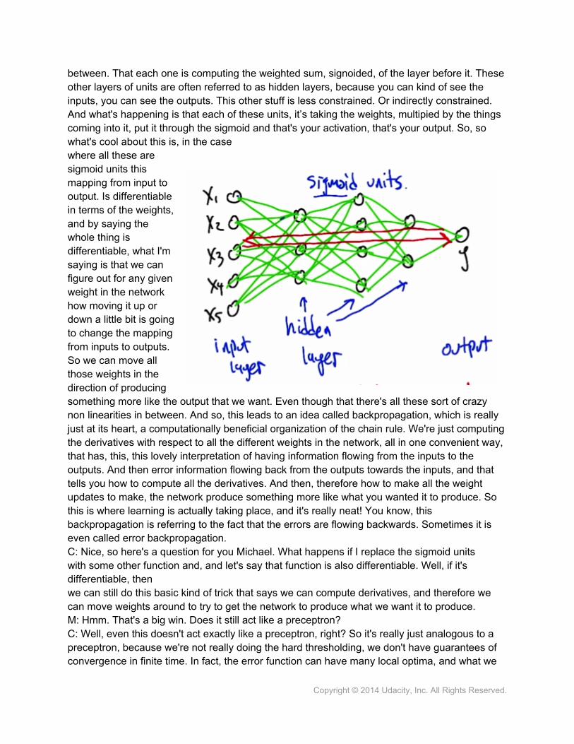
M: Alright so we're now in a great position to talk about what the network part of the neural network is about. So now the idea is that we can construct using exactly these kind of sigmoid units, a chain of relationships between the input layer, which are the different components of x, with the output. Y, and the way this is going to happen is, there's u, other layers of, of units in
between. That each one is computing the weighted sum, signoided, of the layer before it. These other layers of units are often referred to as hidden layers, because you can kind of see the inputs, you can see the outputs. This other stuff is less constrained. Or indirectly constrained. And what's happening is that each of these units, it’s taking the weights, multipied by the things coming into it, put it through the sigmoid and that's your activation, that's your output. So, so what's cool about this is, in the casewhere all these are sigmoid units this mapping from input to output. Is differentiable in terms of the weights, and by saying the whole thing is differentiable, what I'm saying is that we can figure out for any given weight in the network how moving it up or down a little bit is going to change the mapping from inputs to outputs. So we can move all those weights in the direction of producing something more like the output that we want. Even though that there's all these sort of crazy non linearities in between. And so, this leads to an idea called backpropagation, which is really just at its heart, a computationally beneficial organization of the chain rule. We're just computing the derivatives with respect to all the different weights in the network, all in one convenient way, that has, this, this lovely interpretation of having information flowing from the inputs to the outputs. And then error information flowing back from the outputs towards the inputs, and that tells you how to compute all the derivatives. And then, therefore how to make all the weight updates to make, the network produce something more like what you wanted it to produce. So this is where learning is actually taking place, and it's really neat! You know, this backpropagation is referring to the fact that the errors are flowing backwards. Sometimes it is even called error backpropagation.C: Nice, so here's a question for you Michael. What happens if I replace the sigmoid units with some other function and, and let's say that function is also differentiable. Well, if it's differentiable, thenwe can still do this basic kind of trick that says we can compute derivatives, and therefore we can move weights around to try to get the network to produce what we want it to produce.M: Hmm. That's a big win. Does it still act like a preceptron?C: Well, even this doesn't act exactly like a preceptron, right? So it's really just analogous to a preceptron, because we're not really doing the hard thresholding, we don't have guarantees of convergence in finite time. In fact, the error function can have many local optima, and what we
mean by that is this idea that we're trying to set the weight so that the error is low, but you can get to these situations where none of the weights can really change without making the error worse. And you'd like to think we're done. We've made the error as low as we can make it, but in fact it could actually just be stuck in a local optima, that there's a much better way of setting the weights It's just we have to change more than just one weight at a time to get there.M: Oh so that makes sense, so if we think about the sigmoid and the error function that we picked right. The error function was sum of squared errors, so that looks like a parabola in some high dimensional space, but once we start combining them with others like this over and over again then we have an error space where there may be lots of places that look low but only look low if you're standing there but globally would not be the lowest point.C: Right, exactly right and so you can get these situations in just the one unit version where the error function as you said is this nice little parabola and you can move down the gradient and when you get down to the bottom you're done. But now when we start throwing these networks of units together we can get an error surface that looks just in its cartoon form looks crazy like this, that there's, it's smooth but there's these places where it goes down, comes up again and goes down maybe further, comes up again and doesn't come down as far and you could easily get yourself stuck at a point like this where you're not at the global minimum. Your at some local optimum.
Optimizing Weights
M: So one of the things that goes wrong, when you try to actually run gradient descent on a complex network with a lot of data is that you can get stuck in these local minima and then you start to wonder, boy is there some other way that I can optimize these weights. I'm trying to find a set of weights for the neural network that tries to minimize error on the training set. And so, gradient descent is one way to do it, and it can get stuck, but there's other kinds of advanced optimization methods that become very appropriate here. And in fact, there's a lot of people in machine learning who think of optimization and learning as kind of being the same thing. What you're really trying to do in any kind of learning problem is solve this high order, very difficult optimization problem to figure out what the the learned representation needs to be. So, I need to mention in passing some kinds of advanced methods that people have brought to bear, there's things like using momentum terms in the gradient, which basically, where the idea in momentum is, as we're doing gradient descent. So let's imagine this is our error surface, we don't want to get stick on this ball here, we want to kind of pass all the way through it to get to this ball, so maybe we need to just continue in the direction we've been going. So, instead of thinking of it as a kind of physical analogy. Instead of just going to the bottom of this hill and getting stuck, it can kind of bounce out and pop over and come to, what might be a lower, minima, later. There's a lot of work in using higher order derivatives to, to better optimize things instead of just thinking about the, way that individual weights change the error function to look at combinations of weights. Hamiltonions and what not. There's various ideas for randomized optimization, which we're going to get to in a sister course, that can be applied to, to, to make things more robust. And sometimes it's worth thinking, you know what, we don't really want to just minimize the error on the training set, we may actually want to have some kind of penalty for using, using a structure that's too complex. I mean this, this ,uh, when did we, when did we see something like
this before Charles?C: When we were doing regression, and we were talking about over fitting.M: So right. That's right. It came up in regression but something similar will also happen in the decision tree section.C: Sure. We, we had a, we had a issue with decision trees where if we had, we let the tree grow too much to explain every little quirk in the data. You'd overfit. We came up with a lot of ways of dealing with that, like pruning. Not going too far deeply into the tree. You can either do that by filling out the tree and then backing up so you only have a little bit of small error Or by stopping once you've reached some sort of threshold as you grow the tree out. That's really the same as giving some kind of penalty for complexity.M: Yes, exactly, right. So complexity in the tree setting has to do with the size of the tree, in regression it had to do with the order of the polynomial. What do you suppose it would mean in the neural net setting? And, and how would you predict, what negative attributes it might have. So, what's, what's a more or less complex network?C: Well, there's two things you can do with networks, you can add more and more nodes, and you can add more and more layers.M: Good. So, right. So the more nodes that we put into network, the more complicated the mapping becomes from input to output, the more local minima we get, the more we have the ability to actually model the noise, which brings up exactly the same overfitting issues. It turns out there's another one that's actually really interesting in the neural net setting which, I think didn't occur to people in the early days but it became clear and clear over time, which is that , you can also have a complex network, just because the numbers, the weights, are very large. So same number of weights, same number of nodes, same number of layers, but larger numbers often leads to more complex networks and the possibility of overfitting. Sometimes we want to penalize a network not just by giving it fewer nodes or layers but also by keeping the numbers in a reasonable range. Does that make sense?C: Makes perfect sense.
Restriction Bias
M: So this brings up the issue of what neural nets are more or less appropriate for. What is the restriction bias, and the inductive bias of this class of classifiers, and regression algorithms? So Charles, can you remind us what restriction bias is?C: Well, restriction bias Tells you something about the representational power of whatever data structure it is that you're using. So in this case the network of neurons. And it tells you the set of hypotheses that you're willing to consider.M: Right, so if there's a great deal of restriction, then there's lots and lots of different kinds of models that we're just not even considering. We're, we're restricting our view to just a subset of those. So In the case of neural nets, what restrictions are we putting?C: Well, we started out with a simple perceptron unit, and that we decided was linear. So we were only considering planes. Then we move to networks, so that we could do things like XOR, and that allowed us to do more. Then we started sticking Sigmoids and other arbitrary functions and to nodes so that we could represent more and more, and you mention that if you let weights get big and we have lots of layers and lots of nodes they can be really complex. So, it seems
to me that we are actually not doing much of a restriction at all. So let me ask you this then Michael. What kind of functions can we represent, clearly we can represent boolean functions, cause we did that. Can we represent continuous functions? That's a great question to ask, that's what we should try to figure that out. So, in the case, as you said, Boolean functions, we can. If we give ourselves a complex enough network with enough units, we can basically map all the different sub components of any Boolean expression to threshold like units and basically build a circuit that can compute whatever Boolean function we want. So that one definitely can happen. So what about continuous functions? So what is it? What is a continuous function? A continuous function is one where, as the input changes the output changes somewhat smoothly, right? There's no jumps in the function like that.M: Well, there's no discon, there's no discontinuities, that's for sure.C: Alright, now if we've got a continuous function that we're trying to model with a neural network. As long as it's connected, it has no, no discontinuous jumps to any place in the space, we can do this with just a single hidden layer. As long as we have enough hidden units, as long as there's enough units in that layer. And, essentially one way to think about that is, if we have enough hidden units, each hidden unit can worry about one little patch of the function that, that it needs to model. And they, the patches get set at the hidden. And at the output layer they get stitched together. And if you just have that one layer you can make any function as long as it's continuous. If it's Arbitrary. We can still represent that in our neural network. Any mapping from inputs to outputs we can represent, even if it's discontinuous, just by adding one more hidden layer, so two total hidden layers. And that gives us the ability to not just stitch these patches at their seams, but also to have big jumps between the patches. So in fact, neural networks are not very restrictive in terms of their bias as long as you have a sufficiently complex network structure, right, so maybe multiple hidden layers and multiple units. So that worries me a little bit Michael, because it means that we're almost certainly going to overfit, right? We're going to have arbitrarily complicated neural networks and we can represent anything we want to. Including all of the noise that's represented in our training set. So, how are we going to avoid doing that?M: Excellent question. So, this is exactly what worries me. But, it is the case though, that when we train neural networks, we typically give them some bounded number of hidden units and we give them some bounded number of layers. And so, it's not like any fixed network can actually capture any arbitrary function. So any fixed network can only capture whatever it can capture, which is a smaller set. So going to neural nets in general doesn'thave much restriction. but any given network architecture actually does have a bit more restriction. So that's one thing, the other is hey, well we can do with overfitting what we've done the other times we've had to deal with overfitting. And that's to use ideas like, cross validation. And we used cross validation to decide. How many hidden layers to use. We can use it to decide how many nodes to put in each layer. And we can also use it to decide when to stop training because the weights have gotten too large. So, and this is, it's probably worth pointing this out that this is kind of a different, different property from the other classes of supervised learning algorithms we've looked at so far. So in a decision tree, you build up the decision tree and you may have overfit. In regression, you solve the regression problem, and again that may have overfit. What's interesting about neural network training is it's this iterative process that you started out running, and as it's running, it's actually errors going down and down. So, in this
standard kind of graph, we get the error on the training set dropping as we increase iterations. It's doing a better and better job of modeling the training data. But, in classic style, if you look at the error in the, in some kind of held-out test set, or maybe in a cross validation set, you see the error starting out kind of high and maybe dropping along with this, and at some point it actually turns around and goes the other way. So here, even though we're not changing the network structure itself, we're just continuing to improve our fit, we actually get this pattern that we've seen before, that the cross validation error can turn around and at this low point, you might want to just stop training your network there. The more you train it, possibly the worse you'll do. It's reflecting this idea that the complexity of the network is not just in the nodes and the layers, but also in the magnitude of the weights. Typically what happens in this turnaround point is that some weights are actually getting larger and larger and larger. So, just wanted to highlight that difference between neural net function approximation of what we see in some of the other algorithms
Preference Bias
M: Alright, you know the issue that we want to make surethat we think about each time we introduce a new kindof supervised learning representation is to ask what its preference biasis. So Charles, can you remind us what preference bias is?C: Mike researcher bias tells you what it is you are able to represent. Preference bias tells you something about the algorithm that you are using to learn. That tells you, given two representations, why I would prefer one over the other. So, perhaps you think back what we talked about with decision trees, we preferred trees where nodes near the top had high information gain We preferred correct trees. We preferred trees that were shorter to ones that were longer unnecessarily and so on and so forth. So that actually brings up a point here which is, we haven't actually chosen an algorithm. We talked about how derivatives work, how backpropagation works, but you missed telling me one very important thing, which is how do we start? You tell me how to update the weights but, how do I start out with the weights? Do they all start at zero? Do they all start out at one? How do you usually set the weights in the beginning? M: Yes indeed. We did not talk about that, that's, it's really important. You can't run this algorithm without initializing the weights to something. Right? We did talk about how you update the weights but they don't just you know, just start undefined and you, you can't just update something that's undefined. So we have to set the initial weights to something. So pretty typical thing for people to do, is small, random, values. So why do you suppose we want random values?C: Because we have no particular reason to pick one set of values over another. So you start somewhere in the space. Probably helps us to avoid local minimum.M: Yea kind of. I mean there's also the issue if we run the algorithm multiple times if we get stuck, we like it not to get stuck exactly there again, if you run it again. So it gives some variability, which is a helpful thing in avoiding local minimal. And what do you suppose, it's important to start with small values.C: Well you just said. In our discussion before that if the weights get really big that can sometimes lead to overfitting, because it let's you represent arbitrarily complex functions.
M: Good. And so, and what is that tell us about what the preference bias is then?C: Well if we start out with small random values. That means we are starting out with low complexity. So that means we prefer Simpler explanations to more complex explanations. And of course the usual stuff like we prefer correct answers to incorrect answers, and so on and so forth.M: So, you'd say that neural networks implement a kind of bias that says prefer correct over incorrect but all things being equal, the simpler explanation, is preferred.C: Well, if you have the right algorithm. If the algorithm starts with small, random values and tries to stop, you know, when you start over-fitting Then you, cause you're going to start out with the simpler explanations first before you allow your weights to grow. so you, about that.M: So this reminiscent of the principal that is known as Occan's razor which is often stated as entities should not be multiplied unnecessarily. And given that we're working with neural networks, there's a lot of unnecessary multiplication that happens. [LAUGH] But, in fact, this actually is referring to exactly what we've been talking about. So this unnecessarily is, one interpretation of this is that, "Well, when is it necessary?" It's necessary if you're getting betterexplanatory power, you're fitting your data better. So unnecessarily would mean, well we're not doing any better at fitting the data. If we're not doing any better at fitting the data, then we should not multiply entities. And multiply here means make more complex. So don't make something more complex unless you're getting better error, or if two things have similar error Choose the simpler one, use the one that's less complex. That has been shown to, if you mathematize this and you use it in the context of supervised learning, that we're going to get better generalization error with simpler hypotheses.