Note on: Methods of theoretical chemistry Prof. Roi Baer Lesson 1: Molecular electric conduction I. The density of states in a 1D quantum wire Consider a quantum system with discrete en- ergy levels , = 1,2, … Take an energy (not necessarily an energy level) and ask: how many states () have an energy less than . One can use the Heavi- side function to answer this (see box on right), and then: () = ∑ ( − ) (1.1) The derivative of the accumulative number of states is the density of states (DOS) at energy : () = ′ (). Clearly: () = ∑ ( − ) (1.2) Since ∫ () ∞ 0 =1 the DOS has the prop- erty that for any smooth function () of the energy: ∫ ()() = ∑ ( ) (1.3) Thus we can replace a summation over the states by integration: ∑ → ∫ (). We never really use delta-functions when we speak of DOS. Almost always there are decay mechanisms that widen these delta spikes. Thus the delta functions are usually replaced by lorentzian functions or gaussians. The Heaviside () and Dirac () functions. These have the property that for any (): ∫ ()( − ) ∞ −∞ =∫ () −∞ ∫ ()( − ) ∞ −∞ = () The first integral shows that the definition of the Heaviside function is: () = 1 > 0 () = 0 ≤ 0 The second integral shows that () is zero for all ≠0 but, putting () = 1: ∫ ( − ) ∞ −∞ =1 Taking the derivative of the 1 st integral wrt of shows the relation between the two functions: ′ () = ()
Transcript
Note on: Methods of theoretical chemistry Prof. Roi Baer
Lesson 1: Molecular electric conduction
I. The density of states in a 1D quantum wire
Consider a quantum system with discrete en-
ergy levels 𝐸𝑛, 𝑛 = 1,2, …
Take an energy (not necessarily an energy
level) 𝐸 and ask: how many states 𝑁(𝐸) have
an energy less than 𝐸. One can use the Heavi-
side function to answer this (see box on right),
and then:
𝑁(𝐸) = ∑ 𝜃(𝐸 − 𝐸𝑛)
𝑛
(1.1)
The derivative of the accumulative number of
states is the density of states (DOS) at energy
𝐸: 𝜌(𝐸) = 𝑁′(𝐸). Clearly:
𝜌(𝐸) = ∑ 𝛿(𝐸 − 𝐸𝑛)
𝑛
(1.2)
Since ∫ 𝛿(𝑥)𝑑𝑥∞
0= 1 the DOS has the prop-
erty that for any smooth function 𝑓(𝐸) of the
energy:
∫ 𝑓(𝐸)𝜌(𝐸)𝑑𝐸 = ∑ 𝑓(𝐸𝑛)
𝑛
(1.3)
Thus we can replace a summation over the states by integration: ∑𝑛 → ∫ 𝜌(𝐸)𝑑𝐸. We
never really use delta-functions when we speak of DOS. Almost always there are decay
mechanisms that widen these delta spikes. Thus the delta functions are usually replaced
by lorentzian functions or gaussians.
The Heaviside 𝜃(𝑥) and Dirac 𝛿(𝑥) functions.
These have the property that for any 𝑓(𝑥):
∫ 𝑓(𝑥)𝜃(𝑦 − 𝑥)𝑑𝑥∞
−∞
= ∫ 𝑓(𝑥)𝑑𝑥𝑦
−∞
∫ 𝑓(𝑥)𝛿(𝑦 − 𝑥)𝑑𝑥∞
−∞
= 𝑓(𝑦)
The first integral shows that the definition of the
Heaviside function is:
𝜃(𝑥) = 1 𝑖𝑓 𝑥 > 0
𝜃(𝑥) = 0 𝑖𝑓 𝑥 ≤ 0
The second integral shows that 𝛿(𝑥) is zero for all
𝑥 ≠ 0 but, putting 𝑓(𝑥) = 1:
∫ 𝛿(𝑦 − 𝑥)𝑑𝑥∞
−∞
= 1
Taking the derivative of the 1st integral wrt 𝑦 of
shows the relation between the two functions:
𝜃′(𝑥) = 𝛿(𝑥)
Note on: Methods of theoretical chemistry Prof. Roi Baer
Let us compute the DOS of an important basic system: a particle on a ring of circumfer-
ence 𝐿. As with any free particle the energy is 𝐸𝑚 =𝑝𝑚
2
2𝜇 where 𝑚 = 0, ±1, ±2, … and 𝑝𝑚
is the linear momentum of the particle corresponding to an angular momentum ℏ𝑚. For a
particle on a ring of radius 𝑎 the angular momentum 𝒓 × 𝒑 is simply 𝑎𝑝. Thus 𝑝𝑚 =
ℏ𝑚
𝐿/2𝜋= 𝑚
ℎ
𝐿. We see that the linear momentum 𝑝𝑚 = 𝑚 × Δ𝑝 is equally spaced where the
spacing is Δ𝑝 =ℎ
𝑚. Compute 𝑁(𝐸). We find the momentum corresponding to 𝐸:
𝑝(𝐸)2
2𝜇= 𝐸 → 𝑝(𝐸) = ±√2𝜇𝐸
And thus the number of states with energy less than 𝐸 is the number of states 𝑚 with
momentum 𝑝𝑚 in the interval −𝑝(𝐸) < 𝑝𝑚 < 𝑝(𝐸). So: 𝑁(𝐸) = 2 × 𝑚(𝐸) − 1 where
𝑚(𝐸) = [𝑝(𝐸)
Δ𝑝] and we use the notation that [𝑥] is the largest integer smaller than 𝑥. If we
think of a long wire, we can imagine that the integer aspect is smoothed out, so we can
write:
𝑁(𝐸) = 2𝐿𝑝(𝐸)
ℎ
The density of states is just the derivative of this. From 𝑝2 = 2𝜇𝐸, and taking derivative
w.r.t. 𝐸 we have 𝑝𝑝′ = 𝜇 so that: 𝜌(𝐸) = 𝑁′(𝐸). Thus, in terms of momentum:
𝜌(𝐸) = 2𝜇𝐿
ℎ𝑝(𝐸)
(1.4)
Note that the density of states is proportional to the length of the wire and inverse prop-
tional to the square root of the energy.
II. Theory of electric conduction through molecules
Consider an electron on the ring discussed above and ask: for a given state 𝑚 what is the
electric current? Since the velocity is 𝑣𝑚 =𝑝𝑚
𝜇, the time the electron completes a rotation
Note on: Methods of theoretical chemistry Prof. Roi Baer
is 𝜏𝑚 =𝐿
𝑣𝑚 and so 𝐼𝑚 =
𝑒
𝜏𝑚=
𝑒𝑣𝑚
𝐿=
𝑒𝑝𝑚
𝜇𝐿. For a long wire we can write these quantities as
functions of 𝐸
𝐼(𝐸) =𝑒
𝜇𝐿𝑝(𝐸) (2.1)
Now, let us try to connect the current and the density of states 𝜌. Using (1.4), we obtain a
relation between the current going left (say) and the density of states of the “wire”:
𝐼(𝐸)𝜌(𝐸) =𝑒
ℎ (2.2)
Note we “lost” a factor 2 because for each energy we consider only the “left” going
states. This relation is remarkable: when an electron is transported through an energy lev-
el 𝐸 of a device, the product of the current by the density of states is independent of 𝐸, of
the electron mass or the wire length! In fact the result is a constant of nature 𝑒
ℎ and is a
purely quantum effect (due to the presence of ℎ)! What does this inverse proportionality
of the current to the density of states mean? It means that wen you calculate the current
resulting from all energy levels in the interval Δ𝐸 Δ𝐸 = 𝐸2 − 𝐸1 then the current is the
simple result:
𝐼(𝐸2, 𝐸1) =𝑒
ℎ∫ 𝐼(𝐸)𝜌(𝐸)𝑑𝐸
𝐸2
𝐸1
=𝑒
ℎ(𝐸2 − 𝐸1) =
𝑒
ℎΔ𝐸
The total current of electrons in an energy range Δ𝐸 is just 𝑒
ℎΔ𝐸: indeed a remarkably
simple rule! This rule is now going to be used to compute the current in a molecular junc-
tion.
Now, consider a wire connected to two electrodes. We focus on “non-interacting elec-
trons”. This means that each electron is independent (except for Pauli principle) from
each other electron. The electrodes inject electrons into the wire and after the electron
passes through the wire it is absorbed by the electrodes. The total current in the wire is
the difference between currents going from the left to the right and from the right to the
left:
𝐼 = 𝐼𝐿→𝑅 − 𝐼𝑅→𝐿 (2.3)
Note on: Methods of theoretical chemistry Prof. Roi Baer
To get the current from left to right we have to sum over all states with positive momen-
tum: 𝐼𝐿→𝑅 = 2 ∑ 𝑤𝑛𝑖𝐿→𝑅𝑅 (𝐸𝑛)𝑛,𝑝>0 where 𝑛 enumerates the states in the left lead and
𝑖𝐿→𝑅𝑅 (𝐸𝑛) is the electric current in the right lead as a result of an impingement of an elec-
tron of energy 𝐸𝑛 coming from the left lead. Note that such an electron coming from the
left can either pass to the right side and contribute to 𝑖𝐿→𝑅𝑅 or to be reflected backwards.
Clearly there is a probability 𝑇(𝐸𝑛) that the impinging electron passes to the right. Be-
cause the number of electrons impinging on the wire coming from left is:
𝑖𝐿→𝑅𝑅 (𝐸) = 𝑤(𝐸)𝑇𝐿→𝑅(𝐸) (
𝑒
ℎ𝜌𝐿(𝐸))
𝑇𝐿→𝑅(𝐸) is a transmission coefficient. 𝑤(𝐸) is the joint probability that the left lead actu-
ally has an electron in state 𝑛 and that on the right the corresponding level of the same
energy is vacant (because of the Pauli principle, if the level is occupied the electron can-
not flow there since a level cannot be occupied by 2 electrons or more). The factor 2
comes from the two possible spin states. Clearly, because electrons are fermions the
population of levels is determined from the Fermi Dirac distributions in the two elec-
trodes, thus:
𝑤(𝐸) = 𝑓𝐿(𝐸)(1 − 𝑓𝑅(𝐸)) (2.4)
Where 𝑓𝑗(𝐸) =1
1+𝑒𝛽(𝐸−𝜇𝑗)
, 𝑗 = 𝐿, 𝑅 is the Fermi-Dirac distribution, 𝜇𝑗 is the chemical
potential of the left or right electrode and (𝑘𝐵𝛽)−1 is the temperature (𝑘𝐵 is Boltzmann’s
constant). All these give:
𝐼𝐿→𝑅 = 2 ∑ 𝑓𝐿(𝐸𝑛)(1 − 𝑓𝑅(𝐸𝑛))𝑖𝐿→𝑅𝑅 (𝐸𝑛)
𝑛,𝑝>0
= 2 ∫ 𝑓𝐿(𝐸)(1 − 𝑓𝑅(𝐸))𝑖𝐿→𝑅𝑅 (𝐸)𝜌𝐿(𝐸)𝑑𝐸
=2𝑒
ℎ∫ 𝑓𝐿(𝐸)(1 − 𝑓𝑅(𝐸))𝑇𝐿→𝑅(𝐸)𝑑𝐸
(2.5)
𝑇𝐿→𝑅(𝐸) is a transmission coefficient. It answers the question: what is the probability that
an electron of energy 𝐸 moving to the right in the left lead ends up in the right lead.
Posed this way, such a question is ill-defined, but it is intuitively clearer.
Note on: Methods of theoretical chemistry Prof. Roi Baer
A similar expression will be used for 𝐼𝑅→𝐿. Thus
𝐼𝑅→𝐿 =2𝑒
ℎ∫ 𝑓𝑅(𝐸)(1 − 𝑓𝐿(𝐸))𝑇𝑅→𝐿(𝐸)𝑑𝐸
(2.6)
We will show in the next section that 𝑇𝑅→𝐿(𝐸) = 𝑇𝐿→𝑅(𝐸) and we thus call both “the
transmission coefficient” 𝑇(𝐸). From Eq. (2.3) we then find:
𝐼 =2𝑒
ℎ∫[𝑓(𝐸 − 𝜇𝐿) − 𝑓(𝐸 − 𝜇𝑅)]𝑇(𝐸)𝑑𝐸
(2.7)
This is Landauer’s equation for the current in a junction. It is very simple. The electronic
structure of the leads and the constriction go in only through the transmission coefficient.
At zero temperature, with no barriers (𝑇(𝐸) = 1) we get the almost similar rule as we
had above:
𝐼 =2𝑒
ℎ(𝜇𝐿 − 𝜇𝑅) =
2𝑒2
ℎΔ𝑉
(2.8)
Where Δ𝑉 = 𝑒−1(𝜇𝐿 − 𝜇𝑅) is the voltage bias between the two electrodes. The conduct-
ance is the derivative of the current by the bias. The conductance in the above case is thus
𝐺 =𝑑𝐼
𝑑Δ𝑉=
2𝑒2
ℎ.
III. 1D model of a molecular junction
We now build a model for a molecular junction. In the junction there are 3 entities: the
molecule, and the left/right metallic leads. Our model will assume that electrons are non-
interacting. This may sound strange, since electrons interact quite strongly, however, it is
well known that a good approximation for the behavior of electronic systems is that by
modifying the overall potential suitably they can be approximately assumed to be non-
interacting. In some phenomena interactions are extremely important, however, such
phenomena are beyond the scope of our treatment.
The model for the molecule is a well, for the present we will assume a square well, but
the methods we develop below are suitable for any shape. So our molecule is schemati-
cally shown in this diagram:
Note on: Methods of theoretical chemistry Prof. Roi Baer
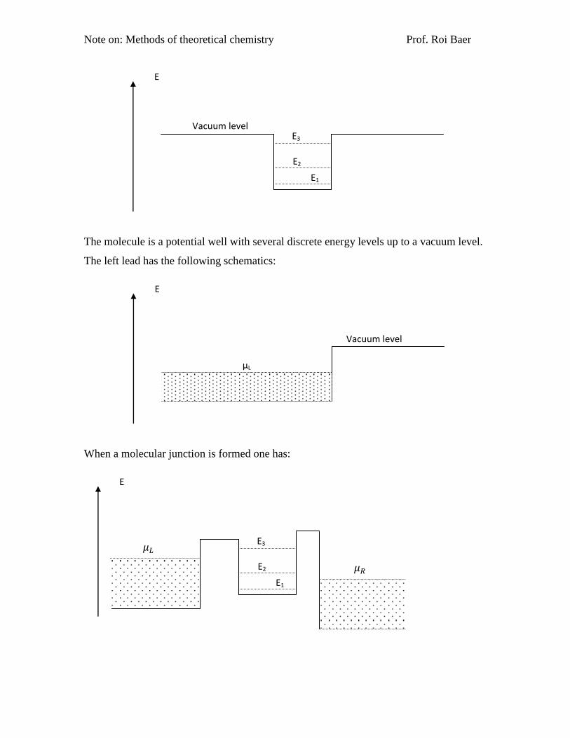
The molecule is a potential well with several discrete energy levels up to a vacuum level.
The left lead has the following schematics:
When a molecular junction is formed one has:
E
Vacuum level
E1
E2
E3
E
Vacuum level
μL
E
E1
E2
E3 𝜇𝐿
𝜇𝑅
Note on: Methods of theoretical chemistry Prof. Roi Baer
Due to the double barrier tunneling phenomenon, we will discuss in the next section, one
can think of conduction as "going through" the energy levels of the molecule (this is a
good assumption when the molecule is weakly coupled to the metal). At zero temperature
one can see in the figure that conductance through molecular level 1 is impossible since
the corresponding energy levels on both sides are occupied (the Fermi-Dirac difference
terms at this energy give zero). In fact due to this, this level of the molecule will itself be
occupied by 2 electrons. I say it is nearly impossible because one can still imagine a pro-
cess in which one electron in level 1 of the molecule will jump up in energy to the lowest
unoccupied state of the right lead (energy 𝜇𝑅) and an electron from the left lead at the
same energy will replace it. But as we shall see in calculations such events have very
small probability since they are essentially tunneling events (violate the energy conserva-
tion for a short period of time). Conduction through level 3 is also nearly impossible for
the same but opposite reason: there are no electrons of energy 𝐸3 in the metals and thus
conductance will occur only through tunneling which has a small probability. However
conduction may occur more readily through level 2 since the left lead can supply elec-
trons that go through the molecule and come out in the vacant levels of the right lead.
IV. Calculating T(E): Transfer Matrix Method
In order to estimate the conductance we need a way to compute the transmission coeffi-
cient in the Landauer formula 𝑇(𝐸). We develop such a method, for 1D systems now.
Consider a potential step, going from potential 𝑉𝐿, 𝑉𝑅 at 𝑥 = 𝑎. The wave functions with
energy 𝐸 on the left and right side of this point are: