(1.1) (1.1) (1.3) (1.3) (1.2) (1.2) Lesson 11: Systems and resultants restart; Real solutions of a system We were looking at the system of equations , where p1 := 2*x^4 - 2*y^3 + y ; p2 := 2 * x^2 * y + 3*y^4 - 2*x ; We had found all the solutions using solve. S:= solve([p1 = 0, p2 = 0], [x,y]); We used allvalues and then evalf to get all the numerical values for the solution that involved RootOf . S2:= evalf([allvalues(S[2])]); Most of the solutions are complex. We just want the real ones (those with no I).
Transcript
(1.1)(1.1)
(1.3)(1.3)
(1.2)(1.2)
Lesson 11: Systems and resultantsrestart;
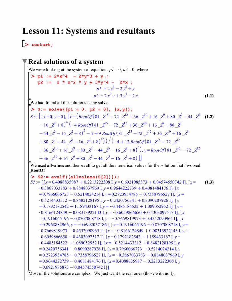
Real solutions of a systemWe were looking at the system of equations , where
p1 := 2*x^4 - 2*y^3 + y ;
p2 := 2 * x^2 * y + 3*y^4 - 2*x ;
We had found all the solutions using solve.S:= solve([p1 = 0, p2 = 0], [x,y]);
We used allvalues and then evalf to get all the numerical values for the solution that involvedRootOf.
S2:= evalf([allvalues(S[2])]);
Most of the solutions are complex. We just want the real ones (those with no I).
(2.3)(2.3)
(2.2)(2.2)
(1.5)(1.5)
(2.1)(2.1)
(1.4)(1.4)
(1.6)(1.6)
remove(has, S2, I);
Here's what's going on in this bit of Maple magic. has(A, B) checks whether a Maple expression A contains a certain subexpression B, returning eithertrue or false. For example:
has(x^2 + y, x);true
has(x^2 + y^3, y^2);false
remove(f, A) takes a function f (which should return either true or false), applies it to each of the operands of A (e.g. the members of a list or set) and removes those where the functions return true,keeping those where it returns false. select(f, A) does the opposite, keeping those where the function returns true. Additional inputs to f can be included in the call to remove or select after the A. Thus in our case, remove(has, S2, I) will evaluate has(t, I) for each of the members of the list S2, and returns the list consisting of those members t for which the result was false, i.e. those that contain only real numbers.
Resultants
What is that polynomial that y is supposed to be a root of?res := resultant(p1,p2,x); factor(res);
This is the resultant of p1 and p2, considered as polynomials in x (with coefficients that are polynomials in y). The most important property is that the resultant of two polynomials is 0 if and only if they have a common root.
To understand resultants, it's simplest to eliminate the distraction of the second variable, and start with polynomials with constant coefficients. I'll take these same polynomials, but fix .
f1 := eval(p1, y=3);
f2 := eval(p2, y=3);
resultant(f1,f2,x);13519230468
Suppose + ... and + ... are polynomials of degrees n and m respectively. In our example, , n = 4, b = 6, m = 2.Let the n roots of be , ..., and the m roots of be , ..., (including repeated roots, if
any). Then the resultant of and is
The symbol
(2.4)(2.4)
(2.6)(2.6)
(1.4)(1.4)
(2.7)(2.7)
(2.8)(2.8)
(2.5)(2.5)
stands for product. We need to multiply all the differences where is a root of
and is a root of , and finally multiply the result by .Note that this will be 0 if and have a root in common.
Let's calculate this for our example, using this definition. First we need the roots.Digits:= 16:
r := fsolve(f1, x, complex);
s := fsolve(f2, x, complex);
OK, four roots for f1 and two for f2. Now to plug in to the formula for the resultant. The mul command will make a sequence of expressions, depending on an index variable, and
multiply them together. For example, for :
mul(c[i],i=1..3);
By the way, for addition we would use add.add(c[i],i=1..3);
In this case I need one mul inside another. 2^2 * 6^4 * mul(mul(r[i]-s[j], j=1..2), i=1..4);
round(%);13519230468
Up to roundoff error, this is the same as what Maple got for the resultant.
Resultant using division
If that was all there was to computing the resultant, it would be rather useless. Fortunately, there arealgebraic ways to calculate it, which don't depend on actually getting the roots, just using the coefficients. This is why it is useful, especially for polynomials in several variables.
Note that
so the resultant of and must be
Similarly, the resultant is also
(3.6)(3.6)
(3.8)(3.8)
(3.1)(3.1)
(3.5)(3.5)
(3.4)(3.4)
(3.7)(3.7)
(1.4)(1.4)
(3.3)(3.3)
(3.9)(3.9)
(3.2)(3.2)
where the comes from the fact that each must be changed to . Let's try these in our example.
2^2 * mul(eval(f2,x=r[i]), i=1..4);
(-1)^8 * 6^4 * mul(eval(f1,x=s[j]), j=1..2);
This would still not be useful if we needed to calculate the roots of one of our polynomials.But now we use division with remainder:Given any two polynomials and , we can write where and are polynomials, and has lower degree than get and using quo and rem.
Q:= quo(f1,f2,x);
f3 := rem(f1,f2,x);
f1 = expand(Q * f2 + f3);
Now the key observation is that , and so (except for the factor , which will have to be adjusted) the resultant of and is the same as the resultant of and .
So instead of calculating the resultant of (of degree 4) and (degree 2), we only have (of degree 1) and to deal with. Next, take the remainder in dividing by .
Now is just a number, so it has no roots at all. The products are just 1, so the resultant of and
is .
resultant(f3,f4,x) = f4^1;
A procedure for the resultantHere's how we could program resultant if we had to, using the ideas from the last section. I'll call itthe procedure MyResultant.
MyResultant:= proc(f1, f2, x)
local a,b,m,n,f3;
m:= degree(f1,x);
a:= coeff(f1,x,m);
n:= degree(f2,x);
b:= coeff(f2,x,n);
if m = -infinity or n = -infinity then 0
elif n = 0 then b^m
elif m = 0 then a^n
elif m < n then
f3:= rem(f2,f1,x);
a^(n-degree(f3,x))*MyResultant(f1,f3,x)
else
f3:= rem(f1,f2,x);
b^(m-degree(f3,x))*MyResultant(f3,f2,x)
end if;
end proc;
(4.2)(4.2)
(1.4)(1.4)
(4.1)(4.1)
Just like resultant, it takes three inputs: two polynomials f1 and f2, and the variable name x. We'll use local variables a, b, m, n and f3. First it finds the degrees m and n of f1 and f2 and the leading coefficients a and b: the coeff command can be used to find those coefficients. Now there are a number of cases to consider, which is taken care of by an if statement.The syntax of the if statement is if conditional expression 1 then statements 1 elif conditional expression 2 then statements 2else statements 3end ifHere's how it works. First it checks conditional expression 1 (which must be something that evaluates to either true or false). If it's true, then Maple executes statements 1 (which can be any number of statements) and then skips to whatever is after the end if. If it's false, then Maple checksconditional expression 2. If that one is true, then Maple executes statements 2 and skips to what's after the end if. Finally, if none of the conditional expressions is true, Maple executes statements 3. The elif clause is optional, and there can be any number of them. The else clause is also optional: if there's no else clause and the conditional expressions are all false, Maple just skips to what's after theend if.In our case, the first conditional expression is m = -infinity or n = -infinity, which would mean f1 orf2 is 0. In that case, the resultant should be 0. The statements 1 just says 0.Since what comes after the end if is end proc, i.e. the end of the procedure, 0 would be the last thing evaluated, so the procedure would return the value 0.If that first conditional expression is not true, Maple tries the second conditional expression n = 0. Ifthat's true, f2 is a nonzero constant, and the result should be b^m. If neither of the first two is true, Maple tries m = 0, and if that's true (i.e. f1 is a nonzero constant) it returns the result a^n.The next thing it tries (if nothing was true yet) is m < n. If that's the case, Maple uses rem to find the remainder in dividing f2 by f1, assigns that to f3, and then returns the appropriate power of a times the resultant of f1 and f3. That is done using this same procedure MyResultant. This means that MyResultant is a recursive procedure: a procedure that calls itself. Finally (if none of the conditional expressions was true), Maple finds the remainder individing f1 by f2, assigns that to f3, and returns the appropriate power of b times the resultant of f3 and f2, again done using a recursive call to MyResultant.Recursive procedures are used very often in Maple. One thing you have to be careful of is that the chain of recursive calls must eventually come to an end. For example, this would be bad:
badproc:= proc(x)
x * badproc(x-1)
end proc;
badproc(10);
Error, (in badproc) too many levels of recursion
In this case the chain didn't come to an end: badproc(10) called badproc(9), which called badproc
(4.4)(4.4)
(4.5)(4.5)
(5.3)(5.3)
(1.4)(1.4)
(4.3)(4.3)
(4.1)(4.1)
(5.1)(5.1)
(5.2)(5.2)
(8), and so on... If you stopped at 1, you'd be computing , but there's nothing to tell Maple to stop there, so it continues with 0, -1, -2, ..., until eventually there are so many recursive calls that Maple stops and gives you an error message. If it didn't do that, it would use up all available memory and crash the computer.Fortunately, this shouldn't be a problem in MyResultant: when the procedure calls itself recursively, it does so with a new polynomial f3 of lower degree than either of f1 and f2. Eventually we must get a polynomial of degree 0 or , at which point the chain stops.Now let's test out MyResultant, comparing its result to Maple's resultant.
MyResultant(f1,f2,x) = resultant(f1,f2, x) ;
MyResultant(p1,p2, x)=
resultant(p1,p2, x);
expand(%);
It seems to work.I should emphasize that this was just an exercise, not really meant to be a serious replacement for Maple's resultant. If you want the resultant, there's no reason not to use resultant.
The other variableNow back to two equations in two variables. We wanted to solve the equations and
p1,p2;
The resultant of these (considered as polynomials in x) should be a polynomial in y which is 0 exactly when and have a common root.
factor(resultant(p1,p2,x));
There are some technicalities here: what's actually true is that if is a root of the resultant and the coefficients of the highest powers of x in and are nonzero for that value of , then there is some that makes That's not a problem here, because the highest powers of x don't
contain y.Now, what is that x ? In the case , it's easy: you just plug in to the equations and immediately see that is the solution for both. But in general, especially if y can only be represented as a complicated RootOf, you really don't want to have to solve some complicated equation with coefficients involving that RootOf. Fortunately, you don't have to. Consider the process that we used to get the resultant, using division with remainder.
p3:= rem(p1,p2,x);
Since for some polynomial q, the solutions of the system will be exactly the
(5.5)(5.5)
(5.6)(5.6)
(5.4)(5.4)
(5.8)(5.8)
(1.4)(1.4)
(4.1)(4.1)
(5.9)(5.9)
(5.7)(5.7)
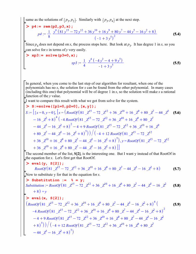
same as the solutions of Similarly with at the next step.
p4:= rem(p2,p3,x);
Since does not depend on x, the process stops here. But look at . It has degree 1 in x, so you can solve for x in terms of y very easily.
xp3:= solve(p3=0,x);
In general, when you come to the last step of our algorithm for resultant, when one of the polynomials has no x, the solution for x can be found from the other polynomial. In many cases (including this one) that polynomial will be of degree 1 in x, so the solution will make x a rational function of the y value. I want to compare this result with what we got from solve for the system.
S:=solve([p1=0,p2=0],[x,y]);
The second member of the list, S[2], is the interesting one. But I want y instead of that RootOf in the equation for x. Let's first get that RootOf.
eval(y, S[2]);
Now to substitute y for that in the equation for x.Substitution := % = y;
eval(x, S[2]);
(5.13)(5.13)
(5.11)(5.11)
(5.15)(5.15)
(5.14)(5.14)
(5.12)(5.12)
(1.4)(1.4)
(4.1)(4.1)
(5.16)(5.16)
(5.10)(5.10)
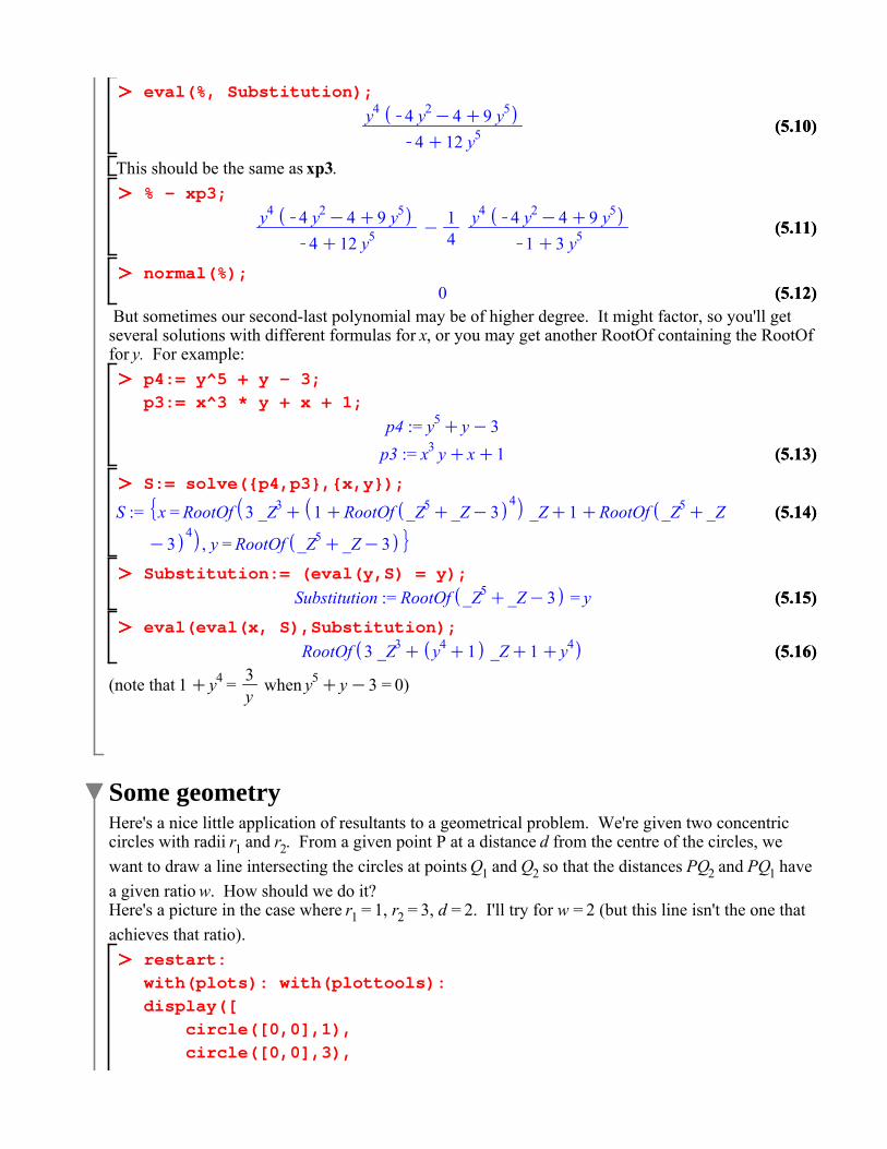
eval(%, Substitution);
This should be the same as xp3.% - xp3;
normal(%);0
But sometimes our second-last polynomial may be of higher degree. It might factor, so you'll get several solutions with different formulas for x, or you may get another RootOf containing the RootOf for y. For example:
p4:= y^5 + y - 3;
p3:= x^3 * y + x + 1;
S:= solve({p4,p3},{x,y});
Substitution:= (eval(y,S) = y);
eval(eval(x, S),Substitution);
(note that when )
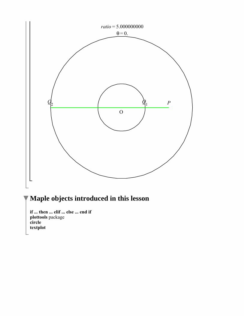
Some geometryHere's a nice little application of resultants to a geometrical problem. We're given two concentric circles with radii and . From a given point P at a distance from the centre of the circles, we want to draw a line intersecting the circles at points and so that the distances and have a given ratio . How should we do it?Here's a picture in the case where , , . I'll try for (but this line isn't the one that achieves that ratio).
A few things to notice about how I drew this picture:The circles were drawn with a command called circle in the plottools package. You tell it the coordinates of the centre of the circle (as a list [x,y]) and the radius. You could also give it acolour option. The default is black.The labels were printed with the textplot command, which is in the plots package. Yougive it a list consisting of x and y coordinates and the text you want it to print, or a list of such lists. I moved the coordinates slightly off the point I wanted to label, because I didn't want the label to be actually on the point. The text to print could be a string (enclosed in quotes), or a Maple expression.The display command is used to put all the pieces together in one plot.I gave the display command the option axes = none, because I didn't want axes interfering with the picture, and scaling = constrained, to make sure the circles look like circles.
(1.4)(1.4)
(4.1)(4.1)
(5.10)(5.10)
(6.1)(6.1)
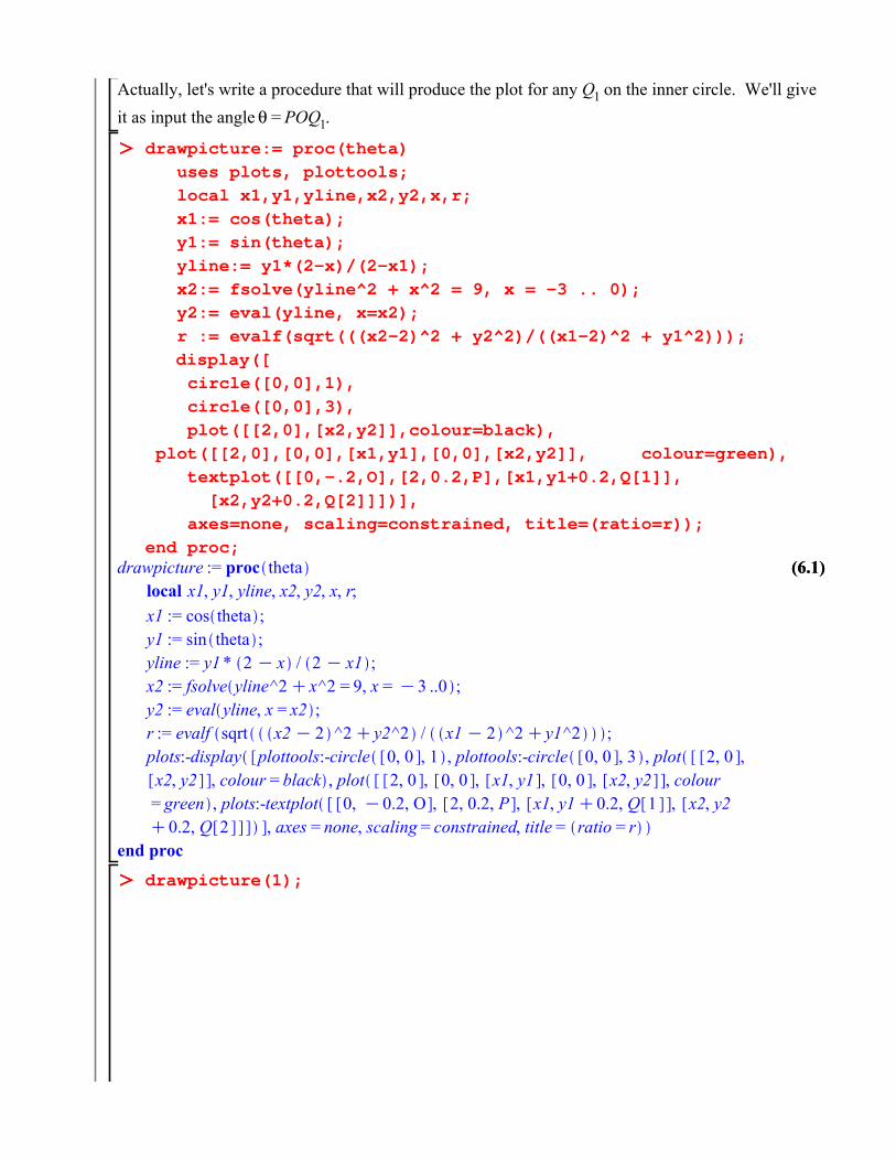
Actually, let's write a procedure that will produce the plot for any on the inner circle. We'll give it as input the angle
drawpicture:= proc(theta)
uses plots, plottools;
local x1,y1,yline,x2,y2,x,r;
x1:= cos(theta);
y1:= sin(theta);
yline:= y1*(2-x)/(2-x1);
x2:= fsolve(yline^2 + x^2 = 9, x = -3 .. 0);
y2:= eval(yline, x=x2);
r := evalf(sqrt(((x2-2)^2 + y2^2)/((x1-2)^2 + y1^2)));