Lesson 15: Building ARMA models. Examples · Lesson 15: Building ARMA models. Examples Umberto...

Lesson 15: Building ARMA models.Examples

Umberto Triacca

Dipartimento di Ingegneria e Scienze dell’Informazione e MatematicaUniversita dell’Aquila,

[email protected]

Umberto Triacca Lesson 15: Building ARMA models. Examples

Examples

In this lesson, in order to illustrate the time series modellingmethodology we have presented so far, we analyze some timeseries.


Example 1

By using a computer program we have generated a time seriesx .The graph of the series is presented in the following figure

Figure : A simulated time series


Example 1

The objective is to build an ARMA model this time series.The first step in developing a model is to determine if theseries is stationary.


Example 1

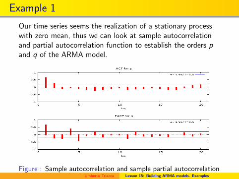
Our time series seems the realization of a stationary processwith zero mean, thus we can look at sample autocorrelationand partial autocorrelation function to establish the orders pand q of the ARMA model.

Figure : Sample autocorrelation and sample partial autocorrelationfunctions of time series xUmberto Triacca Lesson 15: Building ARMA models. Examples

Example 1

Since the SACF cuts off after lag 2 and the SPCAF follows adamped cycle,

an MA(2) model

xt = ut + θ1ut−1 + θ2ut−2, ut ∼ WN(0, σ2)

seems appropriate for the sample data.


Example 1

Table reports the result of the ML estimation.

300 observations, Dependent Variable x

Variabile Coefficient St. error t statistic p-value

θ1 1,68559 0,0456203 36,9481 0,0000θ2 0,883683 0,0492842 17,9303 0,0000

Variance of innovations 0.941107


Example 1

Now, we consider the graph of the residuals

Figure : Residuals from MA(2) model


Example 1

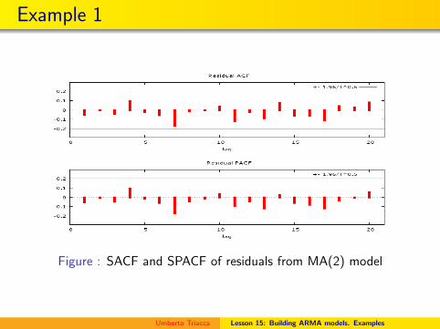
Figure : SACF and SPACF of residuals from MA(2) model


Example 1

By analysing the SACF and SPACF of residuals presented infigure, we note that any term isn’t significant andQ25 = 16.4450 do not indicate any autocorrelation in theresiduals. They can be assimilate to a white noise process.


Example 1

We conclude that the MA(2) model defined by

xt = ut + 1.686ut−1 + 0.884ut−2, ut ∼ WN(0, 0.94)

appear to fit the data very well.


Example 2

Consider the montly series of the foreign exchange rate Liraper US Dollar from Jannuary 1973 until October 1989 (202observations).


Example 2

It can be observed that the series displays a nonstationarypattern with an upward trending behavior.

Figure : Foreign exchange rate Lira per U.S. $ from Jannuary 19t3until October 1989


Example 2

The first difference of the series seems to have a constantmean, although inspection of the graph (see Figure ) suggeststhye variance is an increasing function of time.

Figure : First difference of the foreign exchange rate Lira per USdollar


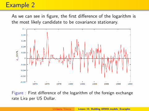
Example 2

As we can see in figure, the first difference of the logarithm isthe most likely candidate to be covariance stationary.

Figure : First difference of the logarithm of the foreign exchangerate Lira per US Dollar.


Example 2

Now, we examine the autocorrelation and partialautocorrelation functions of the logarithmic change in theforeign exchange rate Lira per US Dollar.

Figure : SACF and SPACF for the logarithmic change in theforeign exchange rate Lira per US Dollar.

Examination of the two graphs suggests that an AR(1) modelcan be appropriate. In particular, the SPACF is such thatφ11 = 0.3607 and cuts off to -0.0022 abrutly (i.e.φ22 = −0.0022. Thus the SPACF is suggestive of an AR(1)model.


Example 2

An AR(1) model is fitted by using the exact maximumlikelihood estimation. The parameter estimates aresummarized in the following table


Example 2

Sample 1973:02–1989:10. Dependent Variable: First differenceof log of the foreign exchange rate Lira per US Dollar

Coefficient Std. error t statistic p-value Variance innov.

0,381412 0,0652368 5,8466 0,0000 0,000543700


Example 2

The AR(1) model fit indicates a highly significant parameterφ1 with estimate φ1 = 0, 381.


Example 2

The Q statistic (Q20 = 16, 5014) and the graphs of the SACFand SPACF of residuals (see Figure )indicate that theautocorrelations of the residuals are not statistically significant.

Figure : SACF and SACFP of residuals from the model AR(1)


Example 2

Thus we conclude that the AR(1) model

xt = 0.381xt−1 + ut

where ut ∼ WN(0, 0.00054) and xt is the first difference of logof the foreign exchange rate Lira per US Dollar, fits the datawell.


Example 3

We consider the log of GNP deflator series in USA observedon the period 1955:1- 2000:4. The objective is to build anARMA model for this time series.


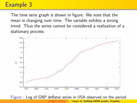
Example 3

The time serie graph is shown in figure. We note that themean is changing over time. The variable exhibts a strongtrend. Thus the series cannot be considered a realization of astationary process.

Figure : Log of GNP deflator series in USA observed on the period1955:1 - 2000:4 Umberto Triacca Lesson 15: Building ARMA models. Examples

Example 3

In order to make stationary the series, we consider the firstdiffereces.

Figure : Graphical plot of the first difference of log of GNPdeflator series


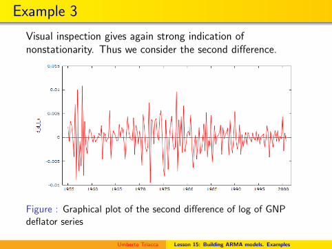
Example 3

Visual inspection gives again strong indication ofnonstationarity. Thus we consider the second difference.

Figure : Graphical plot of the second difference of log of GNPdeflator series


Example 3

The second difference seems the realization of a stationaryprocess with zero mean, thus we can look at sampleautocorrelation and partial autocorrelation function of thesecond difference, to establish the orders p and q of the ARMAmodel. Figure shows the graphs of SACFs and SPACFs.

Figure : Graphical plot of the of SACF and SPACFof the seconddifference of log of GNP deflator series

In this case, it is very difficult to identify the orders p and q ofthe ARMA model by using the correlogram and the partialcorrelogram.


Example 3

Additional information can be obtained by inspecting theoutcomes of the AIC and BIC criteria.

Table : The information criteria: AIC and BIC

Orders p,q of ARMA model2,2 2,1 1,2 1,1 1,0 0,1

AIC -1614.4 -1611.3 -1616.0 -1613.3 -1609.7 -1614.7BIC -1595.2 -1595.2 -1599.9 -1600.4 -1600.1 -1605.1

From AIC values it is concluded that the ARMA(1,2) model ismost suitable for our time series. From BIC values, however,the MA(1) is judged to be better suited.


Example 3

The fact that AIC and BIC provided different indications aboutthe best fitting models is not surprising because BIC penalizeslarger models more than AIC.

Thus BIC tends to produce more parsimonious best-fittingmodels than AIC.


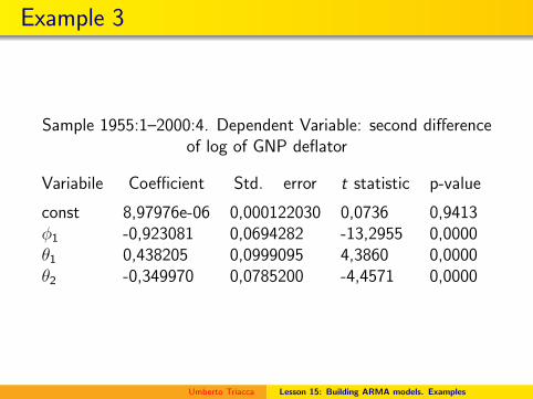
Example 3

Since computing time is inexpensive we can estimate bothmodels. Table 1 shows the results of fitting an ARMA(1,2) forthe second difference of log of GNP deflator.


Example 3

Sample 1955:1–2000:4. Dependent Variable: second differenceof log of GNP deflator

Variabile Coefficient Std. error t statistic p-value

const 8,97976e-06 0,000122030 0,0736 0,9413φ1 -0,923081 0,0694282 -13,2955 0,0000θ1 0,438205 0,0999095 4,3860 0,0000θ2 -0,349970 0,0785200 -4,4571 0,0000


Example 3

Now, we can look at sample autocorrelation and partialautocorrelation functions of residuals of the model ARMA(1,2)to establish if this ARMA model is a good model for the data.

Figure : SACF and SACFP of residuals from the model ARMA(1,2)

These graphs are very similar to the correlograms of a whitenoise process. There is only a SACF coefficient and only aSACFP which are significant. We consider it as a result ofpure chance.


Example 3

The QK -statistic computed with K = 20 lags is equal toQ20 = 16.2932, whereas the critical value isχ2

1−0.05,17 = 27.5871.


Example 3

These results indicate that the ARMA(1,2) model

(1 − 0.923L)xt = (1 + 0.438L− 0.350L2)ut ut ∼ WN(0, 0.85)

with xt = (1 − L)2 log(yt) where yt is the original series, fitsthe data well.


Example 3

Now, we consider the MA(1) model.

Sample 1955:1–2000:4. Dependent Variable: second differenceof log of GNP deflator

Variabile Coefficient Std. error t statistic p-value

const 8,79573e-06 0,000116929 0,0752 0,9400θ1 -0,466072 0,0615454 -7,5728 0,0000


The correlograms and the Box-Pierce statistics(Q20 = 21.6819) indicate that the residuals behave as whitenoise processes.

Figure : SACF and SACFP of residuals from the model MA(1)


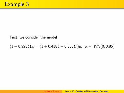
Example 3

Thus we conclude that also the model

xt = (1 − 0.466L)ut ut ∼ WN(0, 0.89),

fits the data well.


Example 3

Let us look at the forecasting performace of the two models.In particular, we forecast the future values of our time series,log(yt), from 2001:1 to 2001:4.


Example 3

First, we consider the model

(1 − 0.923L)xt = (1 + 0.438L− 0.350L2)ut ut ∼ WN(0, 0.85)


Example 3

The 1-step, 2-step, 3-step and 4-step forecasts are presentedin the following table.

Table : ARMA(1,2) forecasts

Step ahead Actual Forecast Std. error2001:1 4,499576 4,498700 0,0029132001:2 4,506344 4,504065 0,0052892001:3 4,509474 4,509945 0,0074032001:4 4,512517 4,515367 0,009934


Example 3

Table presents the forecast obtained by using the MA(1) model

xt = (1 − 0.466L)ut ut ∼ WN(0, 0.89),

Table : MA(1) forecasts

Step ahead Actual Forecast Std. error2001:1 4,499576 4,498286 0,0029562001:2 4,506344 4,503785 0,0054132001:3 4,509474 4,509293 0,0081662001:4 4,512517 4,514810 0,011218


Example 3

Given these results we may conclude that the performance oftwo models is very similar. Which model should be prefered?


Example 3

It is usual to choose a parsimonious model, that is a modelthat describes all of the features of the data of interest usingas few parameters as possible.


Example 3

Thus we choose the MA(1) model

xt = (1 − 0.466L)ut ut ∼ WN(0, 0.89),


Date post:	04-Apr-2018
Category:	Documents
Upload:	doanhanh
View:	220 times
Download:	3 times

Lesson 15: Building ARMA models. Examples · Lesson 15: Building ARMA models. Examples Umberto...

Documents