Lesson 3 – Average Rate of Change and Linear FunctionsLesson 3 – Average Rate of Change and...

Lesson 3 – Average Rate of Change and Linear Functions

89

Lesson 3 – Average Rate of Change and Linear Functions In this lesson, we will introduce the concept of average rate of change followed by a review of linear functions. We will then look at how real world situations can be modeled using linear functions. We will study the relationship between average rate of change and slope and how to interpret these quantities. Finally, we will learn how to create linear models for data sets using linear regression. Lesson Topics: Section 3.1: Average Rate of Change

§ Definition of Average Rate of Change § Comparing Average Rates of Change § Interpreting the Average Rate of Change

Section 3.2: Review of Linear Functions

§ Characteristics and Behavior of Linear Functions § Vertical and Horizontal Intercepts § Interpreting the Slope and Intercepts of a Linear Function § Writing the equation of a line

o Given a Point and a Slope o Given Two Points o Horizontal and Vertical Line

Section 3.3: Modeling with Linear Functions

Section 3.4: Is the Function Linear?

§ Average Rate of Change of a Linear Function § Use the Average Rate of Change to Determine if a Function is Linear

Section 3.5: Scatterplots on the Graphing Calculator Section 3.6: Linear Regression

§ Using Graphing Calculator to Generate a Linear Regression Equation § Using Linear Regression to Solve Application Problems

Lesson 3 – Average Rate of Change and Linear Functions

90

Lesson 3 – Average Rate of Change and Linear Functions - MiniLesson

91

Lesson 3 - MiniLesson

Section 3.1 – Average Rate of Change

The function !C t( ) , whose table is below, gives the average cost, in dollars, of a gallon of

gasoline !t years after 2000 (i.e. !!t =0 corresponds to the year 2000, !!t =1 corresponds to 2001, etc.).

!t 2 3 4 5 6 7 8 9

!C t( ) 1.47 1.69 1.94 2.30 2.51 2.30 3.01 2.14

If we are interested in how gas prices changed between 2002 and 2009, we can see from the table that the cost per gallon increased from $1.47 to $2.14, an increase of $0.67. If we average this increase out over the 7 years from 2002 to 2009, we see that:

Average Change in Cost for a Gallon of Gas from 2002 to 2009 =

096.0yeardollars096.0

767.0$ ≈≈

years dollars per year

Between 2002 and 2009, the price of gas increased at an average rate of about 9.6 cents each year. This example illustrates the mathematical concept of Average Rate of Change.

Average Rate of Change Given any two points !! x1 , f x1( )( )and !! x2 , f x2( )( ) , the average rate of change between the points

on the interval !!x1 to !!x2 is determined by computing the following ratio:

Average rate of change =Inputin Change

Outputin Change =!ΔoutputΔinput 12

12 )()(xxxfxf

−−

Units for the Average Rate of Change are always: !output!unitsinput!unit !,

Units are read as “output units per input unit”

“Δ ” notation denotes change so average rate of change can be thought of as “change in output divided by change in input”

Problem 1 WORKED EXAMPLE – Average Rate of Change Using the same table and information as in the introductory problem above, determine the Average Rate of Change of

!C t( ) from 2002 to 2009 using the formula for Average Rate of

Change.

Average Rate of Change = !!C 9( )− C 2( )

9 − 2 = 2.14 − 1.477 = 0.677 ≈0.096 dollars per year


92

Problem 2 MEDIA EXAMPLE – Average Rate of Change The function

!C t( ) below gives the average cost, in dollars, of a gallon of gasoline !t years after

2000. Find the average rate of change for each of the following time intervals. Interpret the meaning of your answers.

!t 2 3 4 5 6 7 8 9

!C t( ) 1.47 1.69 1.94 2.30 2.51 2.30 3.01 2.14

a) 2003 to 2008

b) 2006 to 2009

c) 2005 to 2007

Problem 3 YOU TRY – Average Rate of Change Jose recorded the average daily temperature,

!D n( ) (in degrees Fahrenheit), for his science class

during the month of June in Scottsdale, Arizona. The table below represents the highest temperature on the nth day of June for that year. (!!n=1 is June 1, !!n=2 is June 2, and so on.) Show all of your work for each of the following and be sure to include correct units in your answers.

!n 1 2 4 6 9 11

!D n( ) 97 98 97 99 104 102

a) Find the average rate of change between !!n= !1 and !!n= !11 . Write a sentence explaining the meaning of your answer.

b) Find the average rate of change between !!n= !9 and !!n= !11 . Write a sentence explaining the meaning of your answer.


93

Problem 4 MEDIA EXAMPLE – Average Rate of Change Average yearly attendance at Arizona Cardinals football games increased from 62,603 in 2011 to 65,832 in 2014 (source: http://www.espn.com/nfl/attendance). Assuming that this growth was linear, determine the average rate of change of attendance during this time period and write a sentence explaining its meaning in the context of this problem. Be sure to use proper units. Problem 5 YOU TRY – Average Rate of Change You opened a savings account and deposited $50 to start your savings account. Each month, you deposited money into that account after paying bills and other expenses. At the end of 8 months, you had saved $526. Assuming that the growth of your savings account was linear, determine the average rate of change of your savings during this time period and write a sentence explaining its meaning in the context of this problem. Be sure to use proper units.


94

Problem 6 MEDIA EXAMPLE – Comparing Average Rates of Change The total sales, in thousands of dollars, for three companies over 4 weeks are shown below. Total sales for each company are clearly increasing, but in very different ways. To describe the behavior of each function, we can compare its average rate of change on different intervals.

Company A: !A t( )

Company B: !B t( )

Company C: !C t( )

AROC

!A t( ) !

B t( ) !C t( )

a)

[0,1]

b)

[1,2]

c)

[2,3]

d)

[3,4]

e) What do you notice about the values above for each function? What do these values tell you about each function?

A function is linear if the rate of change is constant.


95

Section 3.2 – Review of Linear Functions A linear function is a function whose graph produces a straight line. Linear functions can be written in the form!!f x( ) =mx !+ !b , or equivalently!!f x( ) = b+ !mx , where !b is the initial or starting value of the function (also called the vertical intercept), and !m is the slope of the function. [Note: We will see later in the lesson that Slope and Average Rate of Change are interchangeable terms for linear functions].

Important Things to Remember about Linear Functions:

!!f x( ) = !mx !+ !b!!!!!!!!!!!! f x( ) = !b!+ !mx

• !x represents the input variable.!!f (x) represents the output variable.

• The graph of !!f (x) is a straight line with slope, !m , and vertical intercept !!(0,b) .

• Given any two points !! x1 , f x1( )( )and !! x2 , f x2( )( ) , on the graph of !!f (x) ,

!!slope!m= Change!in!OutputChange!in!Input! =

f (x2)− f (x1)x2 − x1

• If !!m> !0 , the graph increases from left to right, If!!m< !0 , the graph decreases from left to right, If!!m= !0 , then !

f x( ) is a constant function, and the graph is a horizontal line.

• The domain of a linear function is generally all real numbers unless a context or situation is applied in which case we interpret the practical domain in that context or situation.

Problem 7 WORKED EXAMPLE – Determine Slope and Vertical Intercept

Equation Slope Behavior Vertical Intercept a) !!f x( ) = −2x + 5 !−2 Decreasing (0, 5)

b) !!r n( ) =2– n !−1 Decreasing (0, 2)

c) !!g x( ) = 34 x + 2

43 Increasing (0, 2)

d) !!k t( ) = 4t 4 Increasing (0, 0)

e) !!f x( ) = −6 0 Constant (0,!−6 )

f) !!x = 4 DNE Vertical Line DNE


96

Horizontal Intercept !! a,0( )

The horizontal intercept is the ordered pair with coordinates !! a,0( ) . The value !a is the input value that results in an output of 0. Problem 8 WORKED EXAMPLE – Find The Horizontal Intercept for a Linear Equation

Find the horizontal intercept for the equation !!f x( ) =2x – !5 .

Replace the value of !!f (x) with 0 then solve for the value of !x .

!!

0=2x −55=2x52 = x

The horizontal intercept is !52 ,0

⎛⎝⎜

⎞⎠⎟= 2.5,0( )

Problem 9 MEDIA EXAMPLE – Find The Horizontal Intercept for a Linear Equation For each of the following problems, find the horizontal intercept and write as an ordered pair.

a)!!f x( ) = –2x + 5 b) !!r n( ) =2– n c) !!g x( ) = 34 x + 2

d) !!k t( ) = 4t e)!!f x( ) = –6!!!!!!!! f) !!x = −3 Problem 10 YOU TRY – Characteristics of Linear Functions Complete the table below showing all work. Write intercepts as ordered pairs. Write answers as simplified fractions.

Equation Slope / Behavior Vertical Intercept Horizontal Intercept

!!A x( ) = 35 x − 8


97

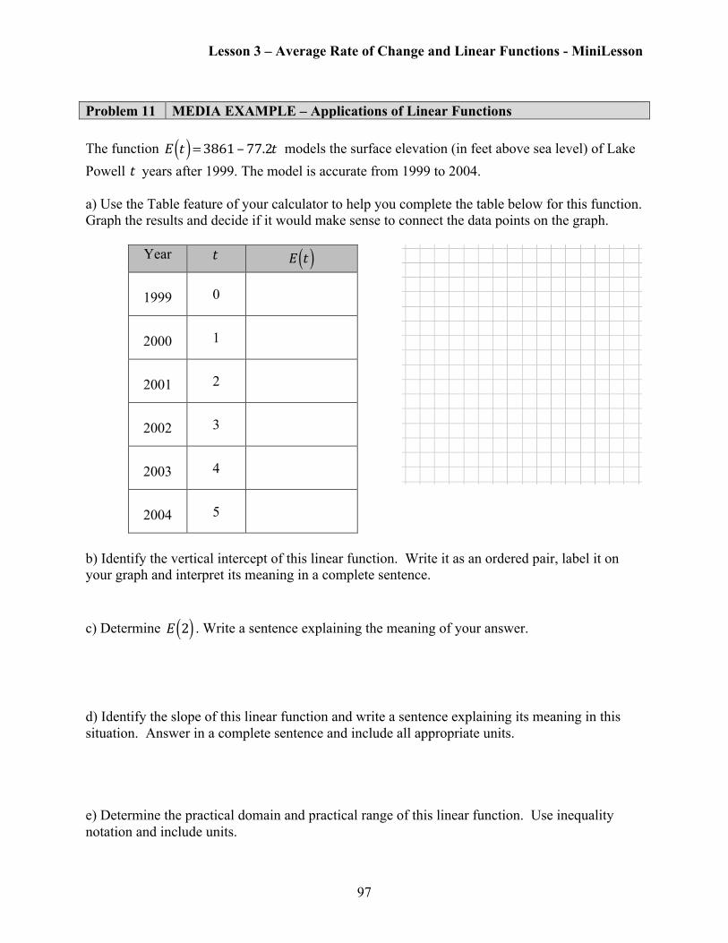
Problem 11 MEDIA EXAMPLE – Applications of Linear Functions The function !!E t( ) =3861–77.2t !models the surface elevation (in feet above sea level) of Lake Powell !t years after 1999. The model is accurate from 1999 to 2004. a) Use the Table feature of your calculator to help you complete the table below for this function. Graph the results and decide if it would make sense to connect the data points on the graph.

Year !t !E t( )

1999 0

2000 1

2001 2

2002 3

2003 4

2004 5

b) Identify the vertical intercept of this linear function. Write it as an ordered pair, label it on your graph and interpret its meaning in a complete sentence.

c) Determine !!E 2( ) . Write a sentence explaining the meaning of your answer.

d) Identify the slope of this linear function and write a sentence explaining its meaning in this situation. Answer in a complete sentence and include all appropriate units.

e) Determine the practical domain and practical range of this linear function. Use inequality notation and include units.


98

Problem 12 YOU TRY – Applications of Linear Functions The linear function !!B n( ) =20000 − 4000n models the amount in your college savings account as a function of the number of semesters, !n , that you have attended school. a) Use the Table feature of your calculator to help you complete the table below for this function. Graph the results and decide if it would make sense to connect the data points on the graph.

!n !!B(n)

0

1

2

3

4

5

b) Identify the vertical intercept of this linear function. Write it as an ordered pair, label it on your graph and interpret its meaning in a complete sentence.

c) Identify the horizontal intercept of this linear function. Write it as an ordered pair, label it on your graph and interpret its meaning in a complete sentence.

d) Identify the slope of this linear function and interpret its meaning in a complete sentence.

e) Determine the practical domain and practical range of this linear function. Use inequality notation and include units.


99

Problem 13 MEDIA EXAMPLE – Applications of Linear Functions The graph below shows Sally’s distance from home over a 30 minute time period.

a) Identify the vertical intercept. Write it as an ordered pair, label it on your graph and interpret its meaning in a complete sentence. b) Identify the horizontal intercept. Write it as an ordered pair, label it on your graph and interpret its meaning in a complete sentence. c) Determine the slope. Interpret its meaning in a complete sentence.

d) Determine the practical domain of this linear function. Use inequality notation and include units.

e) Determine the practical range of this linear function. Use inequality notation and include

units.


100

Problem 14 MEDIA EXAMPLE – Writing Equations of Lines For each of the following, find the equation of the line that meets the indicated criteria. Leave your answer in slope intercept form if possible. a) Slope !!m= −4 passing through the point (6, !−3).

b) Passing through the points (!−2 , !−3) and (4,!−9) c) Horizontal line passing through (–3, 5) and vertical line passing through (–3, 5). d) Line parallel to the line found in part b but passing through the point (3, 4). e) Line perpendicular to the line found in part b but passing through the point (3, 4).


101

Problem 15 WORKED EXAMPLE – Writing Equations of Lines Write an equation of the line that contains points (–4, –3) and (2, 6) Step 1: Find the slope: Use the ordered pairs (–4, –3) and (2, 6) to compute slope.

!!m= 6 − (−3)2− (−4) =

96 =

32

Step 2: Find the Vertical Intercept: Because neither of the given ordered pairs is the vertical intercept, !b must be computed. Pick one of the given ordered pairs. Substitute !m and the ordered pair into!!f x( ) ! = !mx +b . Solve for !b .

Using (–4, –3)

!!

−3= 32 −4( ) + b−3= −6 + b3= b

or

Using (2, 6)

!!

6= 32 2( ) + b6=3+ b3= b

Step 3: Write the final equation in Slope-Intercept form:

Substitute !!m= 32!and!b=3

into!f x( ) =mx + b to get the final answer:

!!f (x)= 32 x + 3

Problem 16 YOU TRY – Writing Equations of Lines For each of the following, find the equation of the line that meets the indicated criteria. Leave your answer in slope intercept form. Show your work. a) Find the equation of the line passing through (1,4) and (3, –2).

b) Find the equation of the line parallel to !!f x( ) = 23 x − 1 and passing through (3,4).

c) Find the equation of the line perpendicular to !!f x( ) = 23 x − 1 and passing through (4,3).


102

Section 3.3 – Modeling with Linear Functions Problem 17 WORKED EXAMPLE – Modeling with Linear Functions Marcus currently owns 200 songs in his iTunes collection. Every month, he adds 15 new songs. Write a linear function model for the number of songs in his collection, !

N t( ) , as a function of the time in months, !t . How many songs will he own at the end of a year?

Marcus currently owns 200 songs, which is the starting point. This gives the ordered pair (0, 200) which means 200 is the vertical intercept. If he adds 15 songs per month to his collection, then the next ordered pair is (1, 215). To write the linear function, we must find the slope:

!!m= 215 − 2001 − 0 = 151 =15

With the slope and vertical intercept, we can write the function: !!N t( ) =200 + 15t .

With this function we can predict how many songs he will have in 1 year (12 months):

!!

N 12( ) =200 + 15 12( )=200 + 180=380

Marcus will have 380 songs in his collection at the end of one year.

There is something critical to notice in the example above. If the question had been, “find the average rate of change of !

N t( )on the interval from [0,1]” then we would have worked the problem this way:

!!Average!Rate!of!Change=

N 1( ) − N 0( )1 − 0 = 215 − 2001 − 0 = 151 =15

Notice that the outcomes are the same…slope computed in the example above and average rate of change computed here. If you look closely, you will see that the formulas for slope and for average rate of change really are the same…therefore slope and average rate of change quantities are interchangeable in problems. This will be illustrated in the examples that follow. In the meantime, just remember the important concept below:

Slope and Average Rate of Change If a function is linear, then the average rate of change for the function on a given interval is the slope of the linear function on that interval.


103

Problem 18 MEDIA EXAMPLE – Modeling with Linear Functions A new charter school opened with 831 students enrolled. Using correct notation, write a linear function model for the number of students, !

N t( ) , enrolled in the school after !t years, assuming that the enrollment: a) Increases by 32 students per year b) Decreases by 20 students per year

c) Decreases by 100 students every 4 years d) Remains constant each year Problem 19 YOU TRY – Modeling with Linear Functions You just bought a new Sony 55” 3D television set for $2300. The TV’s value decreases at a rate of $250 per year. Construct a linear function model to represent the value of the TV over time in years. Clearly indicate what your variables represent and show your work.


104

Problem 20 MEDIA EXAMPLE – Modeling with Linear Functions In 2004, a school population was 1001. By 2008, the population had grown to 1697. Assume the population is changing linearly. Show your work for each of the following. a) Find a linear function model for the population of the school as a function of years after 2004. Clearly indicate what your variables represent. b) Interpret the slope of this linear function. Write your answer as a complete sentence. c) Identify the vertical intercept of this linear function. Write it as an ordered pair and interpret its meaning in a complete sentence. d) Use your model to predict the population of the school in 2016. Show your work.


105

Problem 21 YOU TRY – Modeling with Linear Functions Working as an insurance salesperson, Jose earns a base salary and a commission on each new policy. Jose’s weekly income depends on the number of new policies that he sells during the week. Last week he sold 3 new policies, and earned $760 for the week. The week before, he sold 5 new policies, and earned $920. a) Construct a linear function model to represent this situation. Clearly indicate what your variables represent. Show your work.

b) Interpret the slope of this linear function. Write your answer in a complete sentence.

c) Interpret the vertical intercept of this linear function. Write your answer in a complete sentence.

d) Assuming the accuracy of the model continues for additional weeks, how much could Jose expect to earn in a week in which he sold 8 new policies? Show your work. Write your answer in a complete sentence.


106

Section 3.4 – Is the Function Linear?

Average Rate of Change of a Linear Function

• If a function is linear, then the average rate of change will be the same between any pair of points.

• If a function is linear, then the average rate of change is the slope of the linear function.

Problem 22 MEDIA EXAMPLE – Is the Function Linear? Determine if the functions, represented in the tables below, are linear. If the function is linear, give the slope and vertical intercept. Then and write the equation. a)

!x !−4 !−1 2 8 12 23 42

!A x( ) !−110 !−74 !−38 34 82 214 442

b)

!a !−1 2 3 5 8 10 11

!r a( ) 5 !−1 1 11 41 71 89

c)

!x !−4 !−1 2 3 5 8 9

!g x( ) 42 27 12 7 !−3 !−18 !−23


107

Problem 23 MEDIA EXAMPLE – Average Rate of Change and Linear Functions The data below reflect your annual salary for the first four years of your current job.

Time, !t , in years 0 1 2 3 4 Salary, !S , in thousands of dollars 20.1 20.6 21.1 21.6 22.1

a) Identify the vertical intercept for the function !

S t( ) . Write it as an ordered pair and interpret its meaning in a complete sentence. b) Determine the average rate of change for !

S t( ) during this 4-year time period. Write a sentence explaining the meaning of the average rate of change in this situation. Be sure to include units. c) Verify that the data represent a linear function by computing the average rate of change between at least two additional pairs of points. d) Write the linear function model for the data. Use the indicated variables and proper function notation.


108

Problem 24 YOU TRY – Average Rate of Change The data below show a person’s body weight during a 5-week diet program.

Time, !t , in weeks 0 1 2 3 4 5 Weight, !W , in lbs 196 192 193 190 190 186

a) Identify the vertical intercept for !

W t( ) . Write it as an ordered pair and write a sentence explaining its meaning in this situation. b) Compute the average rate of change for !

W t( ) over the entire 5-week period. Write a sentence explaining its meaning in this situation. Be sure to include units. c) Compute the average rate of change between week 1 and week 2. Write a sentence explaining its meaning in this situation. Be sure to include units. d) Compute the average rate of change between week 3 and week 4. Write a sentence explaining its meaning in this situation. Be sure to include units. e) Do the data points in the table define a perfectly linear function? Why or why not? f) On the grid below, draw a GOOD graph of this data set with all appropriate labels. Do not connect the dots! You are creating what is called a Scatterplot of the given data points.


109

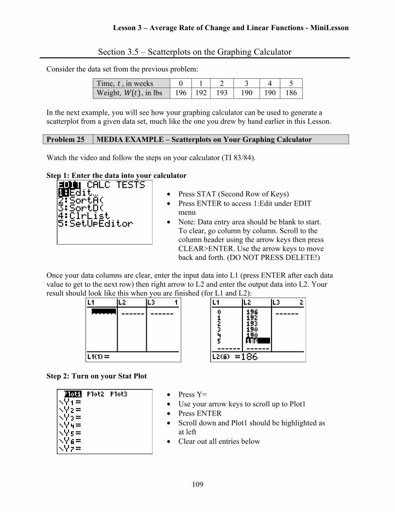
Section 3.5 – Scatterplots on the Graphing Calculator Consider the data set from the previous problem:

Time, !t , in weeks 0 1 2 3 4 5 Weight, !!W(t) , in lbs 196 192 193 190 190 186

In the next example, you will see how your graphing calculator can be used to generate a scatterplot from a given data set, much like the one you drew by hand earlier in this Lesson. Problem 25 MEDIA EXAMPLE – Scatterplots on Your Graphing Calculator Watch the video and follow the steps on your calculator (TI 83/84). Step 1: Enter the data into your calculator

• Press STAT (Second Row of Keys) • Press ENTER to access 1:Edit under EDIT

menu • Note: Data entry area should be blank to start.

To clear, go column by column. Scroll to the column header using the arrow keys then press CLEAR>ENTER. Use the arrow keys to move back and forth. (DO NOT PRESS DELETE!)

Once your data columns are clear, enter the input data into L1 (press ENTER after each data value to get to the next row) then right arrow to L2 and enter the output data into L2. Your result should look like this when you are finished (for L1 and L2):

Step 2: Turn on your Stat Plot

• Press Y= • Use your arrow keys to scroll up to Plot1 • Press ENTER • Scroll down and Plot1 should be highlighted as

at left • Clear out all entries below


110

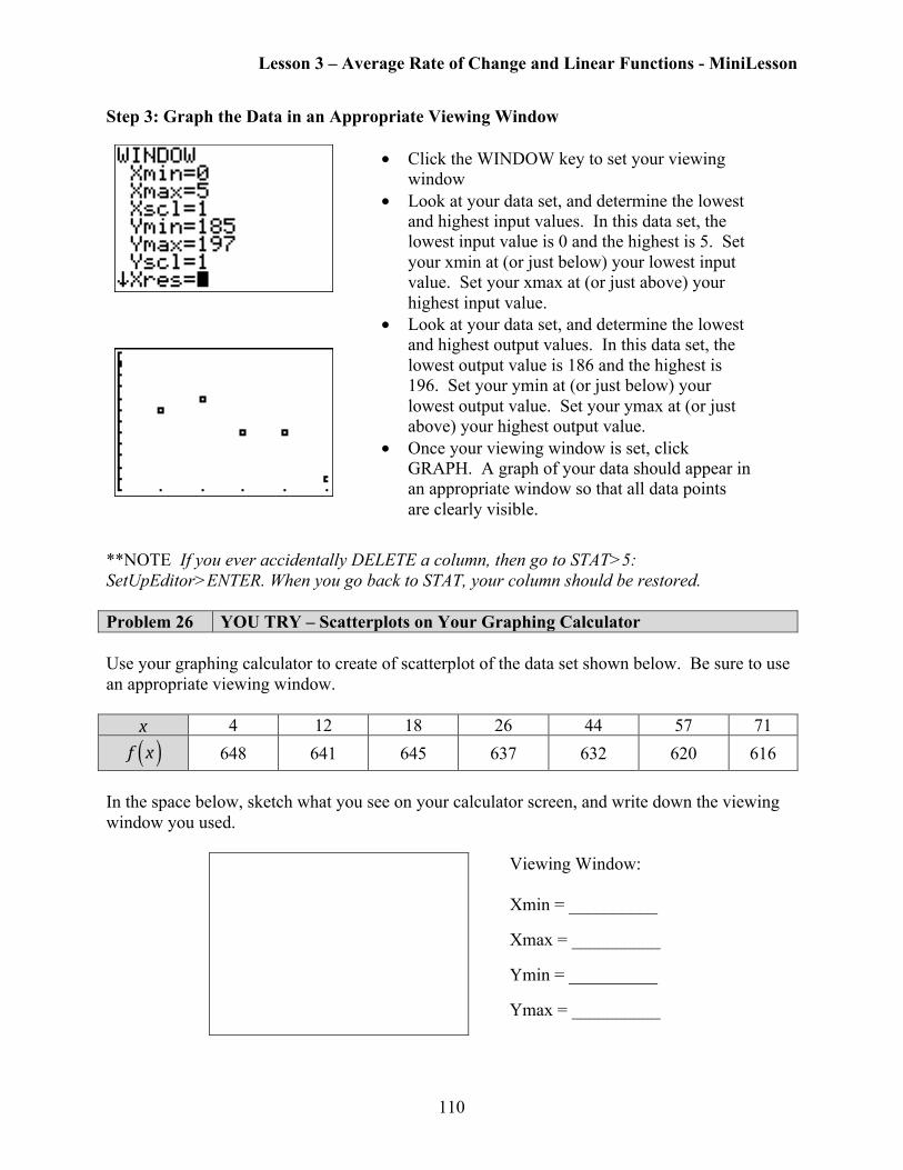
Step 3: Graph the Data in an Appropriate Viewing Window

• Click the WINDOW key to set your viewing

window • Look at your data set, and determine the lowest

and highest input values. In this data set, the lowest input value is 0 and the highest is 5. Set your xmin at (or just below) your lowest input value. Set your xmax at (or just above) your highest input value.

• Look at your data set, and determine the lowest and highest output values. In this data set, the lowest output value is 186 and the highest is 196. Set your ymin at (or just below) your lowest output value. Set your ymax at (or just above) your highest output value.

• Once your viewing window is set, click GRAPH. A graph of your data should appear in an appropriate window so that all data points are clearly visible.

**NOTE If you ever accidentally DELETE a column, then go to STAT>5: SetUpEditor>ENTER. When you go back to STAT, your column should be restored. Problem 26 YOU TRY – Scatterplots on Your Graphing Calculator Use your graphing calculator to create of scatterplot of the data set shown below. Be sure to use an appropriate viewing window.

!x 4 12 18 26 44 57 71

!f x( ) 648 641 645 637 632 620 616

In the space below, sketch what you see on your calculator screen, and write down the viewing window you used.

Viewing Window: Xmin = __________

Xmax = __________

Ymin = __________

Ymax = __________


111

Section 3.6 –Linear Regression Any data set can be modeled by a linear function even those data sets that are not exactly linear. In fact, most real world data sets are not exactly linear and our models can only approximate the given values. The process for writing linear models for data that are not perfectly linear is called linear regression. Statistics classes teach a lot more about this process. In this class, you will be introduced to the basics. This process is also called finding line of the best fit. Problem 27 YOU TRY – The Line of Best Fit Below are the scatterplots of different sets of data. Notice that not all of them are exactly linear, but the data seem to follow a linear pattern. Using a ruler or straightedge, draw a straight line on each of the graphs that appears to fit the data best. This line might not actually touch all of the data points. The first one has been done for you.

a)

b)

c)

d)

To determine a linear equation that models the given data, we could do a variety of things. We could choose the first and last point and use those to write the equation. We could ignore the first point and just use two of the remaining points. Our calculator, however, will give us the best linear equation possible taking into account all the given data points. To find this equation, we use a process called linear regression.


112

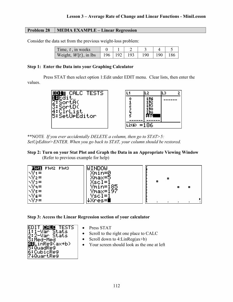
Problem 28 MEDIA EXAMPLE – Linear Regression Consider the data set from the previous weight-loss problem:

Time, !t , in weeks 0 1 2 3 4 5 Weight, !!W(t) , in lbs 196 192 193 190 190 186

Step 1: Enter the Data into your Graphing Calculator Press STAT then select option 1:Edit under EDIT menu. Clear lists, then enter the values.

**NOTE If you ever accidentally DELETE a column, then go to STAT>5: SetUpEditor>ENTER. When you go back to STAT, your column should be restored. Step 2: Turn on your Stat Plot and Graph the Data in an Appropriate Viewing Window (Refer to previous example for help)

Step 3: Access the Linear Regression section of your calculator

• Press STAT • Scroll to the right one place to CALC • Scroll down to 4:LinReg(ax+b) • Your screen should look as the one at left


113

Step 4: Determine the linear regression equation

• Press ENTER twice in a row to view the screen at left

• The calculator computes values for slope (a) and y-intercept (b) in what is called the equation of best-fit for your data.

• Identify these values and round to the appropriate places. Let’s say 2 decimals in this case. So, a = -1.69 and b = 195.38

• Now, replace the a and b in y = ax + b with the rounded values to write the actual equation: y = -1.69x + 195.38

• To write the equation in terms of initial variables, we would write W = -1.69t + 195.38

• In function notation, W(t) = -1.69t + 195.38 Once we have the equation figured out, it’s nice to graph it on top of the scatterplot to see how things match up. GRAPHING THE REGRESSION EQUATION ON TOP OF THE STAT PLOT

• Enter the Regression Equation with rounded values into Y=

• Press GRAPH • You can see from the graph that the “best fit” line

does not hit very many of the given data points. But, it will be the most accurate linear model for the overall data set.

IMPORTANT NOTE: When you are finished graphing your data, TURN OFF YOUR PLOT1. Otherwise, you will encounter an INVALID DIMENSION error when trying to graph other functions. To do this:

• Press Y= • Use your arrow keys to scroll up to Plot1 • Press ENTER • Scroll down and Plot1 should not be highlighted


114

Problem 29 MEDIA EXAMPLE – Linear Regression The function !

f n( ) is defined in the following table.

!n 0 2 4 6 8 10 12

!f n( ) 23.76 24.78 25.93 26.24 26.93 27.04 27.93

a) Based on this table, determine !!f 6( ) . Write the specific ordered pair associated with this

result.

b) Use your graphing calculator to determine the equation of the regression line for the given

data. Round to three decimals as needed.

The regression equation in !!f n( ) ! = an!+ !b form is: ______________________________ c) Use your graphing calculator to generate a scatterplot of the data and regression line on the

same screen. You must use an appropriate viewing window. In the space below, draw what you see on your calculator screen, and write down the viewing window you used.

Xmin=____________ Xmax=____________ Ymin=____________ Ymax=___________

d) Using your regression equation, determine!!f 6( ) . Write the specific ordered pair associated

with this result. e) Your answers for a) and d) should be different. Explain why this is the case.


115

Problem 30 YOU TRY – Linear Regression The function !

C t( ) models the total number of live Christmas trees sold in the U.S., in millions of trees, as function of the number of years since 2004. (Source: Statista.com). Note that the model is only accurate from 2004 to 2011. Sample data points are in the table below.

!t =years since 2004 0 2 4 6 7 Total Number of Christmas

Trees Sold in the U.S. (in millions of trees)

27.1 28.6 28.2 27 30.8

a) Interpret the meaning of the statement !!C 6( ) =27 . Write your answer in a complete sentence. b) Use your calculator to determine the equation of the regression line for !

C t( ) where t represents the number of years since 2004. Use the indicated variables and proper function notation. Round to two decimals as needed. c) Identify the vertical intercept of the regression equation. Write your answer as an ordered pair then use a complete sentence to explain its meaning in the context of this problem. Be sure to use proper units in your response. d) Identify the slope of the regression equation and explain its meaning in the context of this problem. Write your answer in a complete sentence. Be sure to use proper units in your response. e) Use the regression equation to determine !!C 6( ) and explain its meaning in the context of this problem. Is your value the same as the table value from part a)? Why or why not? f) Use the regression equation to predict the number of Christmas trees that will be sold in the year 2013. Show your work and write your answer as a complete sentence.

Date post:	13-Mar-2020
Category:	Documents
Upload:	others
View:	9 times
Download:	0 times

Lesson 3 – Average Rate of Change and Linear FunctionsLesson 3 – Average Rate of Change and...

Documents