Lesson 3 - Linear Functions Introduction As an overview for the course, in Lesson's 1 and 2 we discussed the importance of functions to represent relationships and the associated notation of these functions and we introduced different ways we will work with functions in this course, including Function Arithmetic, Composition and Transformation. In this lesson, we review the most basic type of function, the Linear Functions, and investigate using Linear Functions in Mathematical Modeling and fitting Linear Models to data. OUTLINE Topics Section 3.1 - Linear Functions and Linear Equations Section 3.2 - Average Rate of Change, Slope and the Intercepts Section 3.3 - Special Cases of Linear Functions and Lines Section 3.4 - Linear Applications Section 3.5 - Mathematical Modeling with Linear Functions Section 3.6 - Checking Your Understanding
Transcript
Lesson 3 - Linear Functions
Introduction
As an overview for the course, in Lesson's 1 and 2 we discussed the importance of functions to
represent relationships and the associated notation of these functions and we introduced different
ways we will work with functions in this course, including Function Arithmetic, Composition
and Transformation. In this lesson, we review the most basic type of function, the Linear
Functions, and investigate using Linear Functions in Mathematical Modeling and fitting Linear
Models to data.
OUTLINE
Topics
Section 3.1 - Linear Functions and Linear Equations
Section 3.2 - Average Rate of Change, Slope and the Intercepts
Section 3.3 - Special Cases of Linear Functions and Lines
Section 3.4 - Linear Applications
Section 3.5 - Mathematical Modeling with Linear Functions
Section 3.6 - Checking Your Understanding
Section 3.1 - Linear Functions and Linear Equations
In order to examine linear functions, we will first look at its definition, form and key
characteristics.
Definition:
A linear function is a polynomial function of degree zero or one.
Forms:
Linear Functions are most often expressed in Slope-Intercept Form, which is written as:
Both forms are equivalent. The best choice on which to use is dependent on the context of the
problem.
Characteristic:
Rate of Change:
The defining characteristic of a linear function is the rate of change (slope) of the function.
Because the degree of the function can only be zero or one, the rate of change is always
constant. In other words, increasing the input by one unit will always change the output by
a constant amount.
Graphs:
Because the rate of change is always constant, the graphs of a Linear Function always
result in a nonvertical line. Whether the graph is increasing or decreasing, how quickly it is
increasing or decreasing and where it crosses the vertical axis are determined by the
Coefficients m and b.
The Coefficients m and b:
The value of the coefficient m determines the rate of change.
If m > 0, the function will increase at a constant amount and
the graph of the function will be going up from left to right.
If m < 0, the function will decrease at a constant amount
and the graph of the function will be gong down from left
to right.
If m = 0, the output of the function will always remain the same and the graph will result
in a horizontal line.
The value of the coefficient b determines the vertical intercept. It is the output when the
input is zero. The vertical intercept is always written as an ordered pair (0,b)
Linear Equations:
There are several forms of Linear Equations that are very helpful when working with Linear
Functions and when trying to problem solve Algebraic Applications. Four of them are listed
below.
The Slope-Intercept Form of a Linear Equation
This equation is the same as the Slope-Intercept Form of the Linear Function, without the
use of Function Notation.
The General Form of a Linear Equation
The most common example of the use of this form is when trying to solve Systems of
Equations.
The Point-Slope Form of a Linear Equation
The Point-Slope form of a Linear Equation is useful when given the slope, m and a point
(x1,y1).
The Equation of a Vertical Line
A Linear Function cannot result in a Vertical Line, because one input cannot result in more
than one output. Given that, it is still important that we be able to represent Vertical
Equations and Vertical Lines as part of the problem solving process.
Test Yourself 1 - Slope
Worked Example 1 - Graphs of Linear Functions
The following are four examples of Linear Functions.
Worked Example 2 - Graphs that are NOT Linear Functions
The following are four examples that are NOT Linear Functions.
Test Yourself 2 - Linear Equations
Identify the type of each of the following linear equations.
a. y-3=2(x+8) b. y=2x+4 c. 2x+3y=-8 d. x=-4
Worked Example 3 (Part 1) - Linear Application
Let's take a look at a situation before we look more closely at the characteristics of linear
functions.
Example
• Can you come up with a function that gives your monthly costs as a function of the number of
televisions you make?
• What would the graph of your cost function look like? Why?
We will come back to this example. For now, think about your answers to these questions and
let's take a look at the type of relationship conveyed by a linear function.
Section 3.2 - Average Rate of Change, Slope and the Intercepts
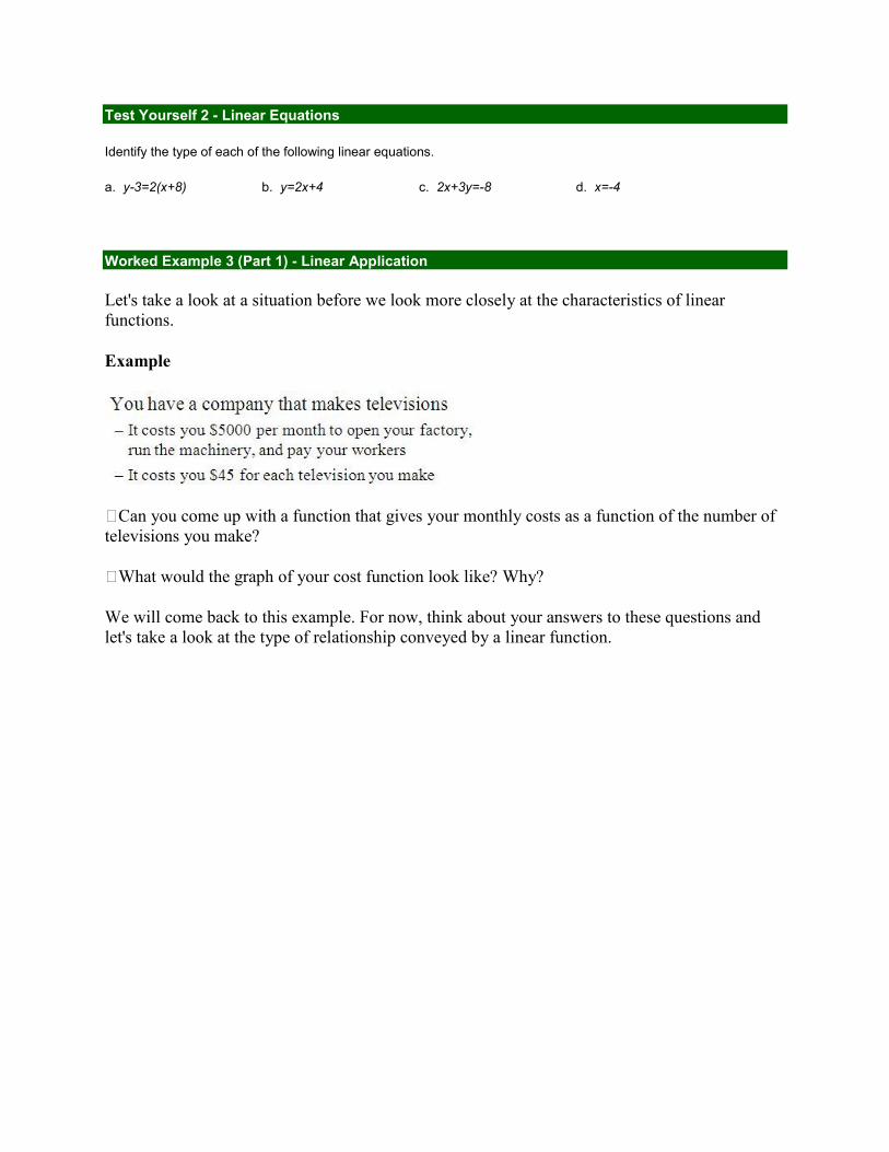
Average Rate of Change of Linear Functions - Slope
The slope IS the constant average rate of change of a linear function. To calculate the slope, or
rate of change, between any two points we do the following:
Now we have alternative notations for slope as well.
Test Yourself 3 - Determining Slope
a. Find the slope between (0,5) and (3,11)
b. True or false? The slope of the line 3x + y = 7 is m=3
c. Find the average rate of change between (3,5) and (5,2)
Intercepts of Linear Functions
In discussing linear functions, it can be useful to know where a graph of a linear function crosses
the vertical and horizontal axes. These are known as the intercepts. There may be both a
horizontal and a vertical intercept. Since x and y are typically used to represent the input and
output, respectively, the intercepts are often called the x-intercepts and y-intercepts.
The vertical intercept (or y-intercept) is where the function crosses the vertical (or y)
axis. This is the output when the input is 0. Thus, it is found by determining the output
value when the input is set to 0. If the linear function is in slope-intercept form, it is the b
value. For example, given the function , when the input is zero (x=0), the
output is 4 and the Vertical Intercept is the ordered pair (0,4)
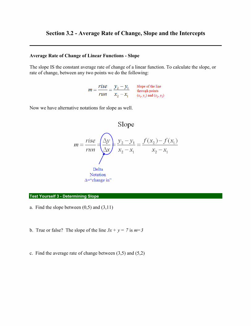
The horizontal intercept (or x-intercept) is where the function crosses the horizontal (or
x) axis. This is the input that yields an output of 0. Thus, it is found by solving for the
input variable when the output variable is set to 0. For example:
Find the Horizontal Intercept of the function
Set
Solve for x
Write the Horizontal Intercept as an ordered pair
Test Yourself 4 - Determining The Vertical and Horizontal Intercept
Find the x and y intercepts of the function 4x - 3y = 24
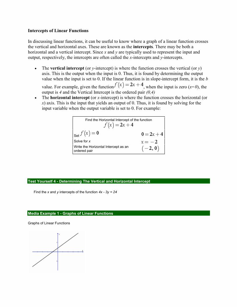
Media Example 1 - Graphs of Linear Functions
Graphs of Linear Functions
Media Example 2 - Linear Equations and Graphs
1. Find the equation of the line passing through the points (0,2) and (5,-3).
2. Sketch the graph.
3. Is the graph increasing, decreasing or neither? That is, as the input increases, does the
output increase, decrease, or neither?
4. How can we answer 3 without looking at the graph?
Average Rate of Change between two points of a Non-Linear Function
It is possible to calculate the Average Rate of Change between two inputs of a Non-Linear Function using the same method as above, but since it is non linear, the slope would vary depending on the inputs chosen..
Worked Example 4 - Average Rate of Change
Two friends are planning to hike to the bottom of the Grand Canyon and back using the Bright Angel Trail and the South Kaibab Trail. They are trying to decide which trail to use to hike down and which to use to hike back out. To help with the decision, they decided to determine which hike has the steeper climb.
Both trails start at the Bright Angel Campground, which is at an elevation of 2480 ft. The Bright Angel Trail is 9.5 miles long and finishes at an elevation of 5729 ft. The South Kaibab Trail is 7 miles long and finishes at an elevation of 6120 ft. Using the same formula for Slope as shown above, we get:
Bright Angel Trail:
South Kaibab Trail:
Given the two calculations, they determine that the average rate of climb for the Bright Angel
Trail is 349.4 feet per mile, while the average rate of climb for the South Kaibab Trail is 520
feet per mile. Meaning that the South Kaibab Trail is almost 50% steeper than the Bright
Angel Trail. Looking at the numbers made it easy. They decided to hike out using the Bright
Angel Trail.
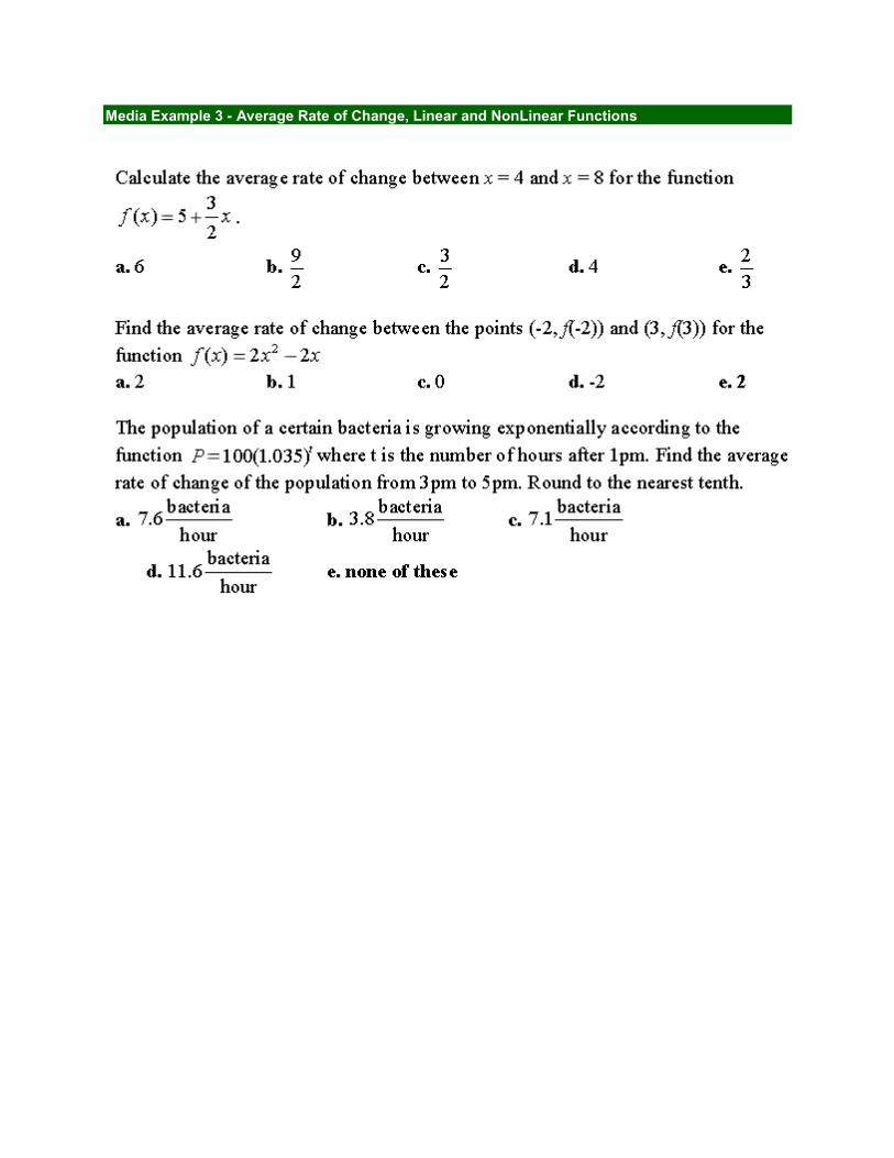
Media Example 3 - Average Rate of Change, Linear and NonLinear Functions
Section 3.3 - Special Cases of Linear Functions and Lines
We have discussed what makes a function linear and what the graph of a linear function looks
like. There are some properties we should discuss that exist in certain situations.
Constant Functions
A constant function has a rate of change of 0.
Vertical Lines
A vertical line has an undefined slope.
Parallel lines
If two lines are parallel, their slopes are equal.
Perpendicular Lines
If two lines are perpendicular, their slopes are opposite reciprocals.
Media Example 4 - Constant Functions and Vertical Lines
Video Notes:
Media Example 5 - Parallel and Perpendicular Lines
Video Notes:
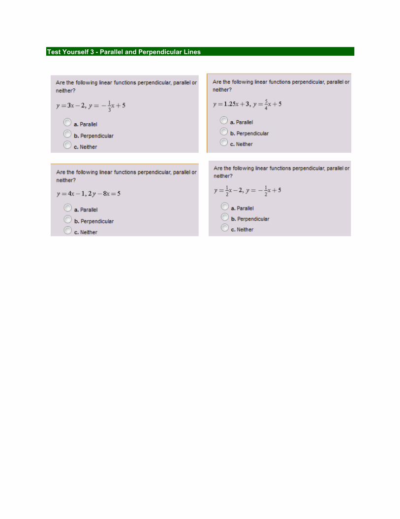
Test Yourself 3 - Parallel and Perpendicular Lines
Section 3.4 - Linear Applications
Worked Example 3 (Continued) - Linear Application
Let's return to our example from earlier.
• Can you come up with a function that gives your monthly costs as a function of the number of
televisions you make?
• What would the graph of your cost function look like? Why?
Solution
If we let C be the total monthly cost in dollars and x be the number of televisions we
produce, then our total monthly cost (in dollars) would be given by C = 45x+ 5000.
Our slope in this case is 45. For each additional television we produce, our total cost will
increase by $45. Thus, we have a constant rate of change of 45 dollars per television
produced.
Our vertical intercept is $5000. This is our overhead cost. It would cost us $5000 per
month if we produced 0 televisions.
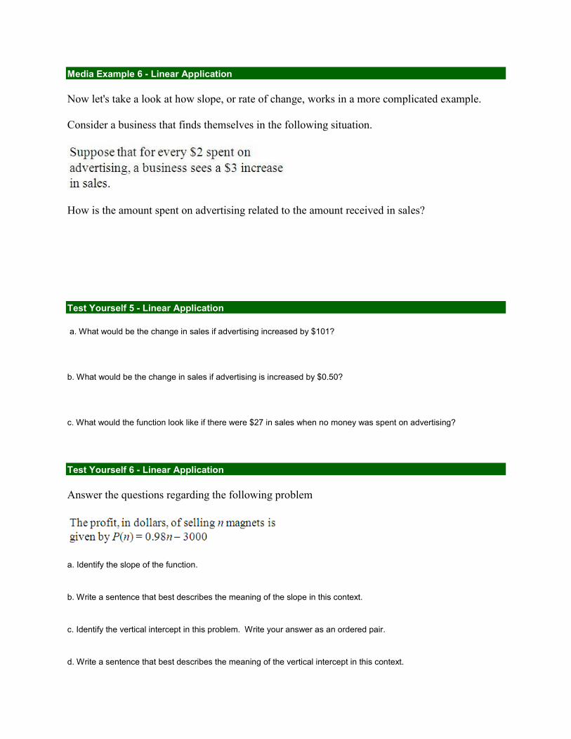
Media Example 6 - Linear Application
Now let's take a look at how slope, or rate of change, works in a more complicated example.
Consider a business that finds themselves in the following situation.
How is the amount spent on advertising related to the amount received in sales?
Test Yourself 5 - Linear Application
a. What would be the change in sales if advertising increased by $101?
b. What would be the change in sales if advertising is increased by $0.50?
c. What would the function look like if there were $27 in sales when no money was spent on advertising?
Test Yourself 6 - Linear Application
Answer the questions regarding the following problem
a. Identify the slope of the function.
b. Write a sentence that best describes the meaning of the slope in this context.
c. Identify the vertical intercept in this problem. Write your answer as an ordered pair.
d. Write a sentence that best describes the meaning of the vertical intercept in this context.
Section 3.5 - Mathematical Modeling with Linear Functions
Since we will be dealing with data during this course, we will need to be able to determine what
function best models our data. For instance, if appropriate, we will use a linear model.
As we build models in this module we will attend to each of these elements. For this section we
are dealing specifically with linear models. How can we determine if our data is linear (or if a
linear model will be a good fit)?
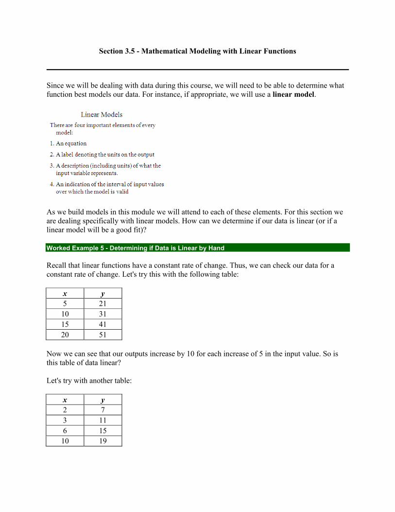
Worked Example 5 - Determining if Data is Linear by Hand
Recall that linear functions have a constant rate of change. Thus, we can check our data for a
constant rate of change. Let's try this with the following table:
x y
5 21
10 31
15 41
20 51
Now we can see that our outputs increase by 10 for each increase of 5 in the input value. So is
this table of data linear?
Let's try with another table:
x y
2 7
3 11
6 15
10 19
Now we can see that our outputs increase by 4 for each row in the table. So is this table of data
linear?
If it is the case that our inputs are equally spaced, we only have to look for a constant difference
in our outputs. If the inputs are not equally spaced, we must calculate the average rate of change
for each interval and compare.
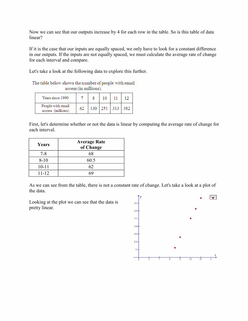
Let's take a look at the following data to explore this further.
First, let's determine whether or not the data is linear by computing the average rate of change for
each interval.
Years Average Rate
of Change
7-8 68
8-10 60.5
10-11 62
11-12 69
As we can see from the table, there is not a constant rate of change. Let's take a look at a plot of
the data.
Looking at the plot we can see that the data is
pretty linear.
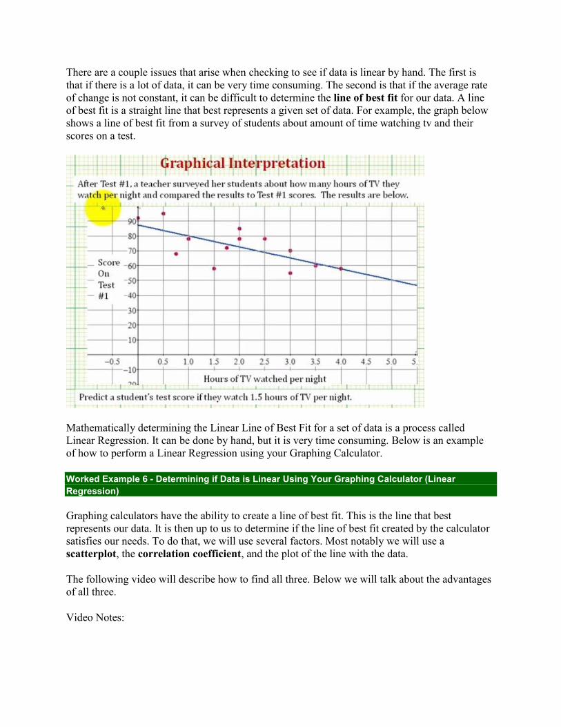
There are a couple issues that arise when checking to see if data is linear by hand. The first is
that if there is a lot of data, it can be very time consuming. The second is that if the average rate
of change is not constant, it can be difficult to determine the line of best fit for our data. A line
of best fit is a straight line that best represents a given set of data. For example, the graph below
shows a line of best fit from a survey of students about amount of time watching tv and their
scores on a test.
Mathematically determining the Linear Line of Best Fit for a set of data is a process called
Linear Regression. It can be done by hand, but it is very time consuming. Below is an example
of how to perform a Linear Regression using your Graphing Calculator.
Worked Example 6 - Determining if Data is Linear Using Your Graphing Calculator (Linear
Regression)
Graphing calculators have the ability to create a line of best fit. This is the line that best
represents our data. It is then up to us to determine if the line of best fit created by the calculator
satisfies our needs. To do that, we will use several factors. Most notably we will use a
scatterplot, the correlation coefficient, and the plot of the line with the data.
The following video will describe how to find all three. Below we will talk about the advantages
of all three.
Video Notes:
Scatterplot
A scatterplot is essentially a plot of our data on axes so we can identify any trends. We already
created one of these for our data above. After watching the previous video, you know how to
create one in your calculator. There are also plenty of programs on the web for creating
scatterplots if you would like to try them. The scatterplot above was created with a program
called Graph available for free at http://www.padowan.dk/graph/.
Correlation Coefficient
The correlation coefficient, r, calculates the "goodness" of our model's fit and will be available
for most of the models we create this semester. It is denoted r and ranges in values between -1
and 1. The closer to -1 or 1, the better the fit. For an exact fit, it would be -1 or 1. It accounts for
how much variation in the output is accounted for by the input. It does not say that the input
causes the output, only that there is a strong relationship (in this case, linear relationship).
You will also notice there is an r² value, this is actually the correlation coefficient squared and
gives us the same information (for our purposes) as r.
Plot
As seen in the video above, we can also compare the plot of the line of best fit with the data
points. This also helps us determine how well the line represents the trend of the data.
Test Yourself 7 - Determining if Data is Linear
Now let's practice with our calculator using the internet user data.
With your calculator find the regression function for the data and answer the following
questions.
a. What is the slope of best fit?
b. Write a sentence that best interprets the meaning of the slope of the line of best fit.
c. What is the vertical intercept of the line of best fit?
d. Write a sentence that best interprets the vertical intercept in this context.
e. What is the correlation coefficient for this model?
d. True or false? The correlation coefficient tells us that this data is NOT very linear.
e. According to the model, how many email users (in millions) were there in 1999?