1 LEVELING RICE ARRIVALS WITH LASER EQUIPMENT: ECONOMIC PERFORMANCE CRITERIA Joseph Maria Franquet Bernis Agricultural Engineer PhD, EUR-ING, Economic and business Sciences PhD, Diploma in Operational Research. Universitat Nacional d’Educació a Distància (UNED). Campus del Nord-est. Centre Associat de Tortosa (Tarragona, Spain). [email protected]. ABSTRACT / SUMMARY Long ago it has been spreading, in our rice-growing areas, the use of leveling laser, allowing farmers a more careful management of irrigation water, enabling a more homogeneous and rational distribution. As a result of the proposed methodology, and based on a real case, it is estimated the surface threshold of profitability of equipment that defines the convenience of its acquisition. In addition, following various microeconomic theory and operational research techniques, it is determined the different curves of cost as well as the optimal period of renewal of the equipment. Key words: leveling, equipment laser, renewal, depreciation, expenditure, break-even point and interest rate. RESUM Des de fa uns quants anys s’ha generalitzat a les nostres zones arrossaires l’ús d’equips d’anivellació làser, que permeten als pagesos el maneig més acurat de l’aigua de reg, possibilitant un reg més homogeni i la utilització de l’aigua de forma més racional. Com a conseqüència de la metodologia aquí proposada, tot partint d’un exemple real, es calcula el llindar superficial de rendibilitat de l’equip a partir del qual resulta interessant la seva adquisició. Endemés, seguint diverses tècniques pròpies de la Teoria Microeconòmica i de la Investigació Operativa es determinen les diferents corbes de cost així com el termini òptim de renovació de l’equip. Paraules clau: anivellament, equip làser, renovació, amortització, despesa, llindar de rendibilitat, tipus d’interès.
Transcript
1
LEVELING RICE ARRIVALS WITH LASER EQUIPMENT: ECONOMIC PERFORMANCE
CRITERIA
Joseph Maria Franquet Bernis Agricultural Engineer PhD, EUR-ING, Economic and business Sciences PhD, Diploma in Operational Research. Universitat Nacional d’Educació a Distància (UNED). Campus del Nord-est. Centre Associat de Tortosa (Tarragona, Spain). [email protected].
ABSTRACT / SUMMARY Long ago it has been spreading, in our rice-growing areas, the use of leveling laser, allowing farmers a more careful management of irrigation water, enabling a more homogeneous and rational distribution. As a result of the proposed methodology, and based on a real case, it is estimated the surface threshold of profitability of equipment that defines the convenience of its acquisition. In addition, following various microeconomic theory and operational research techniques, it is determined the different curves of cost as well as the optimal period of renewal of the equipment. Key words: leveling, equipment laser, renewal, depreciation, expenditure, break-even point and interest rate. RESUM Des de fa uns quants anys s’ha generalitzat a les nostres zones arrossaires l’ús d’equips d’anivellació làser, que permeten als pagesos el maneig més acurat de l’aigua de reg, possibilitant un reg més homogeni i la utilització de l’aigua de forma més racional. Com a conseqüència de la metodologia aquí proposada, tot partint d’un exemple real, es calcula el llindar superficial de rendibilitat de l’equip a partir del qual resulta interessant la seva adquisició. Endemés, seguint diverses tècniques pròpies de la Teoria Microeconòmica i de la Investigació Operativa es determinen les diferents corbes de cost així com el termini òptim de renovació de l’equip. Paraules clau: anivellament, equip làser, renovació, amortització, despesa, llindar de rendibilitat, tipus d’interès.
2
RESUMEN Desde hace tiempo se ha venido generalizando, en nuestras zonas arroceras, el empleo de equipos de nivelación láser, que permiten a los agricultores un manejo más cuidadoso del agua de riego, posibilitando una distribución de la misma más homogénea y racional. Como consecuencia de la metodología aquí propuesta, y partiendo de un caso real, se calcula el umbral superficial de rentabilidad del equipo que nos determina la conveniencia de su adquisición. Además, siguiendo diversas técnicas propias de la Teoría Microeconómica y de la Investigación Operativa, se determinan las diferentes curvas de coste así como el período óptimo de renovación del equipo. Palabras clave: nivelación, equipo láser, renovación, amortización, gasto, umbral de rentabilidad, tipo de interés.
INDEX
Page
ABSTRACT-SUMMARY/RESUM/RESUMEN 1. INTRODUCTION ..................................................................................................... 3 2. LEVELING WITH VERSUS LASER EQUIPMENT TRADITIONAL LEVELING......... 4 3. METHODOLOGY..................................................................................................... 5 3.1. Introduction ........................................................................................................... 5 3.2. Bases of calculation .............................................................................................. 5 3.3. Indirect or fixed costs ............................................................................................ 6 3.4. Direct or proportional costs ................................................................................... 6 3.5. Profitability theshold (Breakeven).......................................................................... 9 3.6. Cost curves......................................................................................................... 11 3.7. Optimal period of equipment renewal.................................................................. 15 4. CONCLUSIONS .................................................................................................... 21 BIBLIOGRAPHIC REFERENCES.............................................................................. 22
* * * * *
3
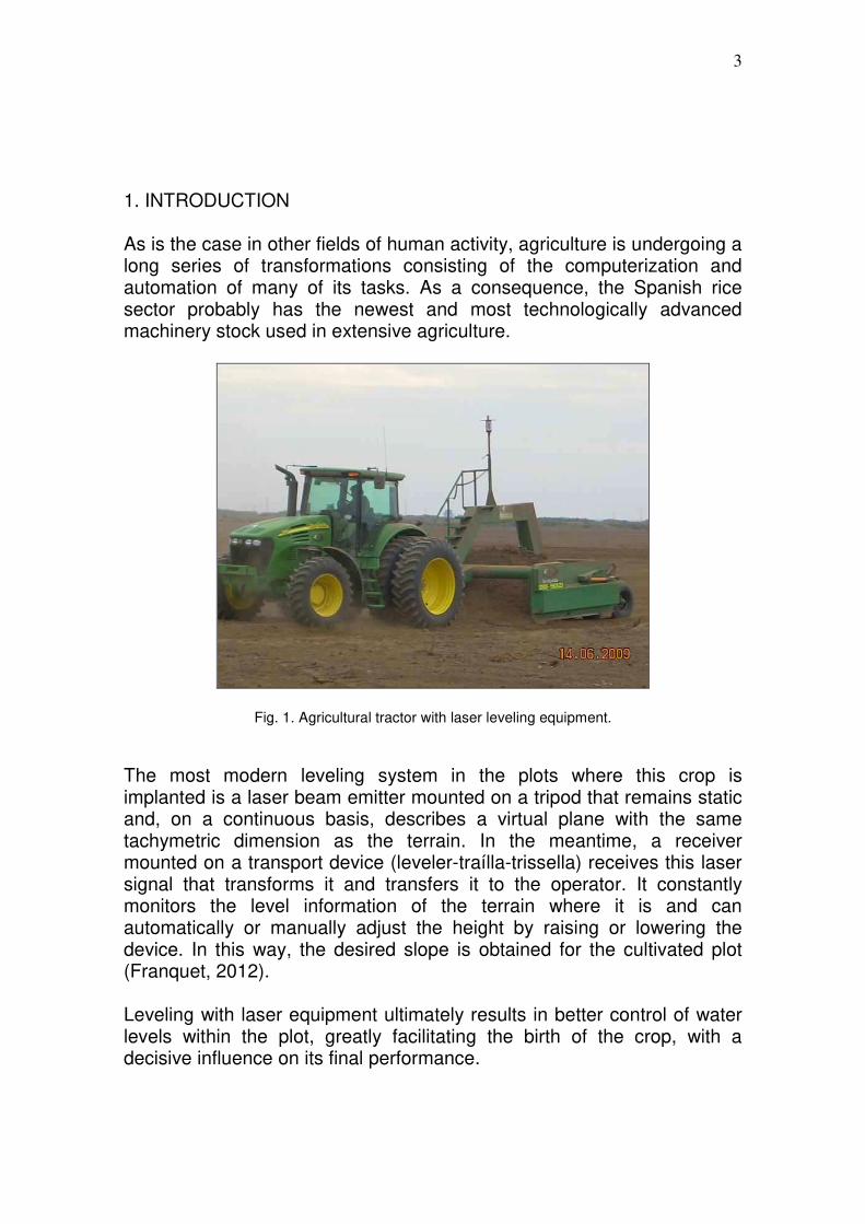
1. INTRODUCTION As is the case in other fields of human activity, agriculture is undergoing a long series of transformations consisting of the computerization and automation of many of its tasks. As a consequence, the Spanish rice sector probably has the newest and most technologically advanced machinery stock used in extensive agriculture.
Fig. 1. Agricultural tractor with laser leveling equipment.
The most modern leveling system in the plots where this crop is implanted is a laser beam emitter mounted on a tripod that remains static and, on a continuous basis, describes a virtual plane with the same tachymetric dimension as the terrain. In the meantime, a receiver mounted on a transport device (leveler-traílla-trissella) receives this laser signal that transforms it and transfers it to the operator. It constantly monitors the level information of the terrain where it is and can automatically or manually adjust the height by raising or lowering the device. In this way, the desired slope is obtained for the cultivated plot (Franquet, 2012). Leveling with laser equipment ultimately results in better control of water levels within the plot, greatly facilitating the birth of the crop, with a decisive influence on its final performance.
4
2. LEVELING WITH VERSUS LASER EQUIPMENT TRADITIONAL LEVELING The traditional leveling of a rice field consists of the following operations: a) Determine the current topographic conditions of the terrain, establishing a grid in the field with a tape measure and a fixed level, leaving permanent stakes in the field to assist in the execution of the work. On one side of each stake is set a level ground level, to which the level will be determined with a fixed level and serves as a reference level during the control of earth movement. b) Carry out the calculation of the plan-project for some variant of the principle of the least ordinary squares (Franquet and Querol, 2010). c) Calculate the construction data (thicknesses of cuts and fillings) and use a system of signalling of these in the field, using the stakes placed in the previous paragraph a). d) Perform the movement of earth with mechanical traction equipment (implements), keeping a control of the construction data (cuts and fills or fills), assisting with support staff, to ensure that the cuts and resultant fillings correspond to the project data (with some preset tolerance). e) Remove the cuttings and give a final leveling with "land plane" when the work of movement of big earth has been accepted. Alternatively, leveling with laser beam equipment such as the one studied here, involves performing the following operations: a) Obtain the current topographic conditions of the terrain, using a transmitting equipment and another laser beam receiver, which may be perfectly the same laser system described above, previously configured to carry out this function. b) Carry out the calculation of the slopes of the project, either in a simplified form or by a variant of the principle of the least squares. c) Perform the earth movement, always guided by the laser system previously configured in order to perform this function. In short, the comparative advantages of laser leveling over traditional leveling are as follows: a) Surveying with laser equipment is carried out in less time, with less staff and less likely to make mistakes. b) Leveling with laser equipment does not require a grid fence through the corresponding altimetric and planimetric lifting of the crop field, as required by traditional leveling. c) Leveling with laser equipment does not require the establishment of a tedious and slow system for controlling construction data in the field.
5
d) The leveling with laser equipment allows to carry out, as much the earth movement as much as the refining or refining of the land, with a high efficiency and precision characteristics of an automatic and electronic system, which translates into a almost perfect work finish. 3. METHODOLOGY 3.1. Introduction It is now a question of calculating the profitability threshold of the laser leveling / refining equipment at a major rice farm, with a territorial base of 669 ha in direct cultivation (in individual farms or in cooperative farms). common use of this modern means of production), while comparing the economic justification of its acquisition with the alternative of renting a similar equipment in the area. It is also required to study and represent the different cost curves and their microeconomic relations, as well as determine the optimal period for equipment renewal (Franquet, 2012). The methodology that follows is applicable to any other example of territorial basis or type of equipment to be acquired. 3.2. Bases of calculation
Acquisition price: C = 35945.94 €
Official subsidy requested: 40% of C.
Actual purchase price: 35945.94 × 0.6 = 21568.00 € Interest on capital: 3%.
Average yield per team: 1.25 h/ha.
Depreciation: it is planned to level every 3 years on the same plot,
so that, for a total direct cultivation area of 669 ha (the rest of the property is in a rustic lease), will correspond to:
×3
ha. 6691.25 h/ha = 278.75 h/year (223 ha/year),
which means approximately 7 weeks of work at the rate of 40 hours/week.
6
3.3. Indirect or fixed costs 3.3.1. Technical depreciation
Amortizable value: 0.9 × 21568.00 € = 19411.20 €, considering a residual value of the equipment of 10% of the initial value.
Machine life: 20 years × 278.75 h/year = 5575 hours.
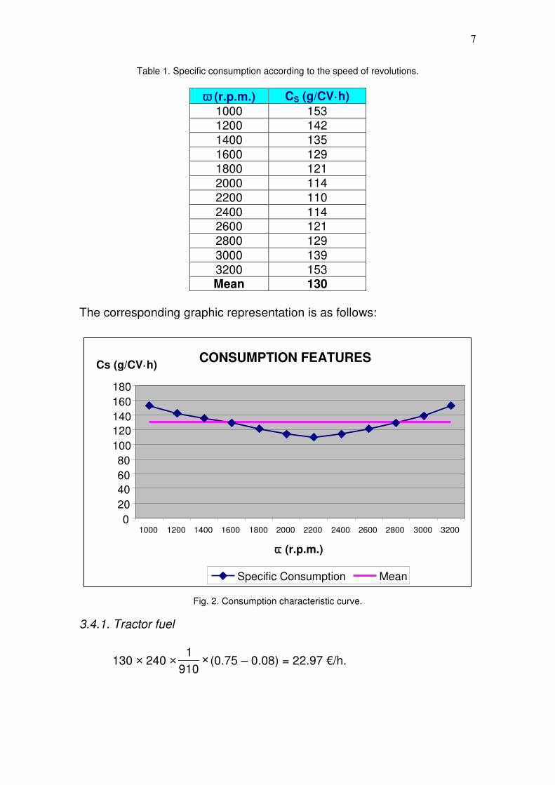
1% s/ 21568.00 = 216 €/year. 3.3.5. Total fixed costs Df = 971 + 647 + 108 + 216 = 1942 €/year. 3.4. Direct or proportional costs 3.4.0. Introduction The predicted laser equipment will be hauled by an agricultural tractor with a power of 240 hp, with an average specific consumption of 130 g/hp as you can see in the following graph, a price of gas of 0.75 €/l with a subsidy of € 0.08/l and a fuel density of 910 g/l. In order to determine the aforementioned value of the average specific consumption, it is necessary to study the corresponding characteristic curves of the Diesel engine at maximum power, which in this case offer the following results,
taking into account the angular velocity (ω) and the specific consumption (Cs):
7
Table 1. Specific consumption according to the speed of revolutions.
ω (r.p.m.) CS (g/CV·h)
1000 153 1200 142
1400 135
1600 129 1800 121
2000 114
2200 110
2400 114 2600 121
2800 129
3000 139
3200 153 Mean 130
The corresponding graphic representation is as follows:
45.71 €/h × 1.25 h/ha = 57.14 €/ha. 3.5. Profitability theshold (Breakeven) As already mentioned, the alternative to the acquisition of the intended laser leveling/refining is to rent the machinery corresponding to the market prices in the studied area, for an approximate amount of currently 60 €/h (year 2015) for this team of 6.00 m shovel width, which represents an expense per surface unit of:
DLL = 60 €/h× 1.25 h/ha = 75.00 €/ha.
DT = DV + N
Df = DLL ; thus:
57.14 + N
1942 = 75.00, where N = 108.73 ha,
demonstrating that from this surface resulting from the previous
calculation (≈109 ha) it is already interesting, from a strictly economic point of view, to invest in the acquisition of the equipment reviewed, whether for individual or joint exploitation. However, each year the leveling and refining of 223 ha is sought (so that each plot of land is leveled approximately every three years), more than the previously calculated surface area, it is concluded that the proposed investment is clearly advisable. Otherwise, the fact that you do not depend on third-party providers to carry out the work, with the delays, uncertainties and difficulties that this entails, further justifies the convenience of making this investment. In this respect, the following table and graph can be viewed:
10
Table 2. Alternative purchase / rent according to the work surface.
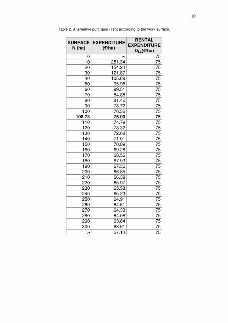
Fig. 3. Calculation of the profitability threshold of the laser equipment.
This curve is an equilateral hyperbola that has two asymptotes or hyperbolic branches, namely (Franquet, 2012):
a) Vertical, for N = 0, that is:
+∞=
+→ N
194214.57lím
0N
b) Horizontal, for N = +∞, that is:
14.57N
194214.57lím
N=
++∞→
.
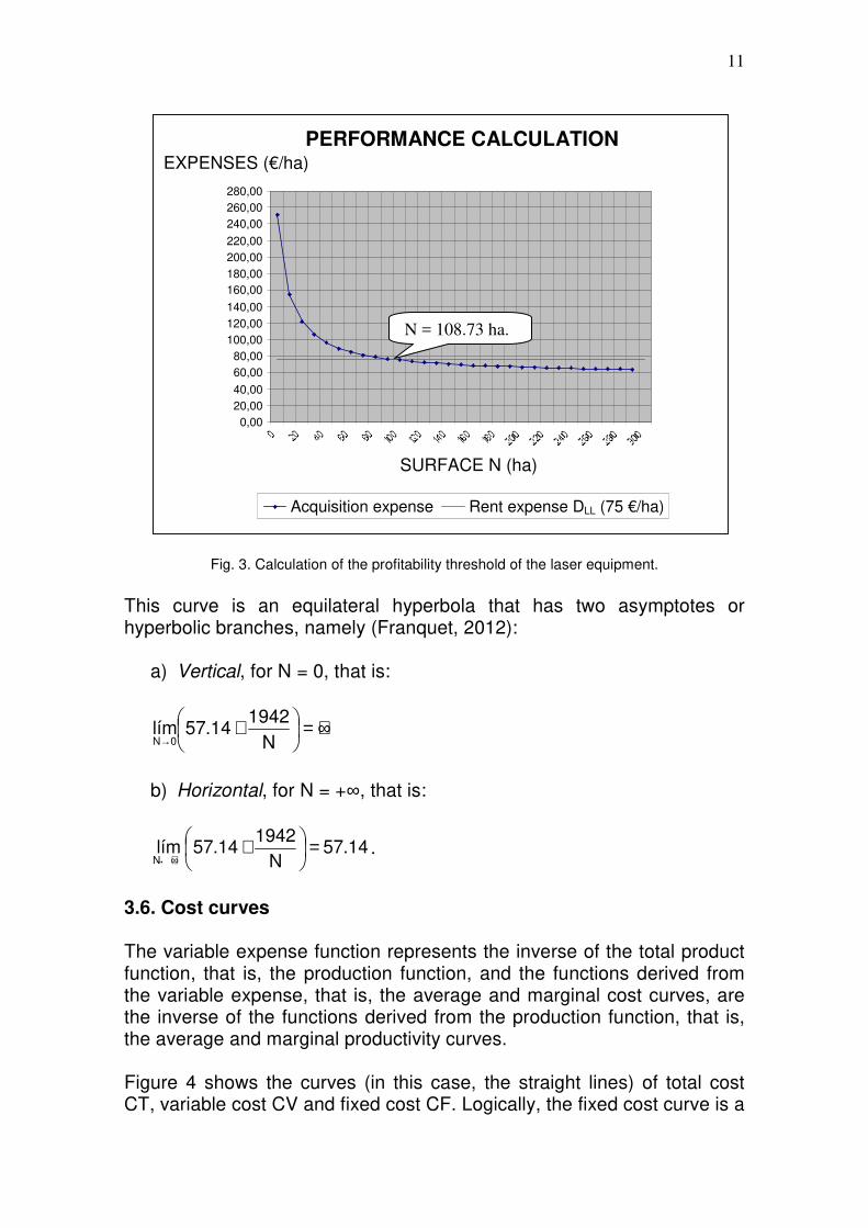
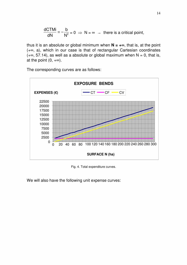
3.6. Cost curves The variable expense function represents the inverse of the total product function, that is, the production function, and the functions derived from the variable expense, that is, the average and marginal cost curves, are the inverse of the functions derived from the production function, that is, the average and marginal productivity curves. Figure 4 shows the curves (in this case, the straight lines) of total cost CT, variable cost CV and fixed cost CF. Logically, the fixed cost curve is a
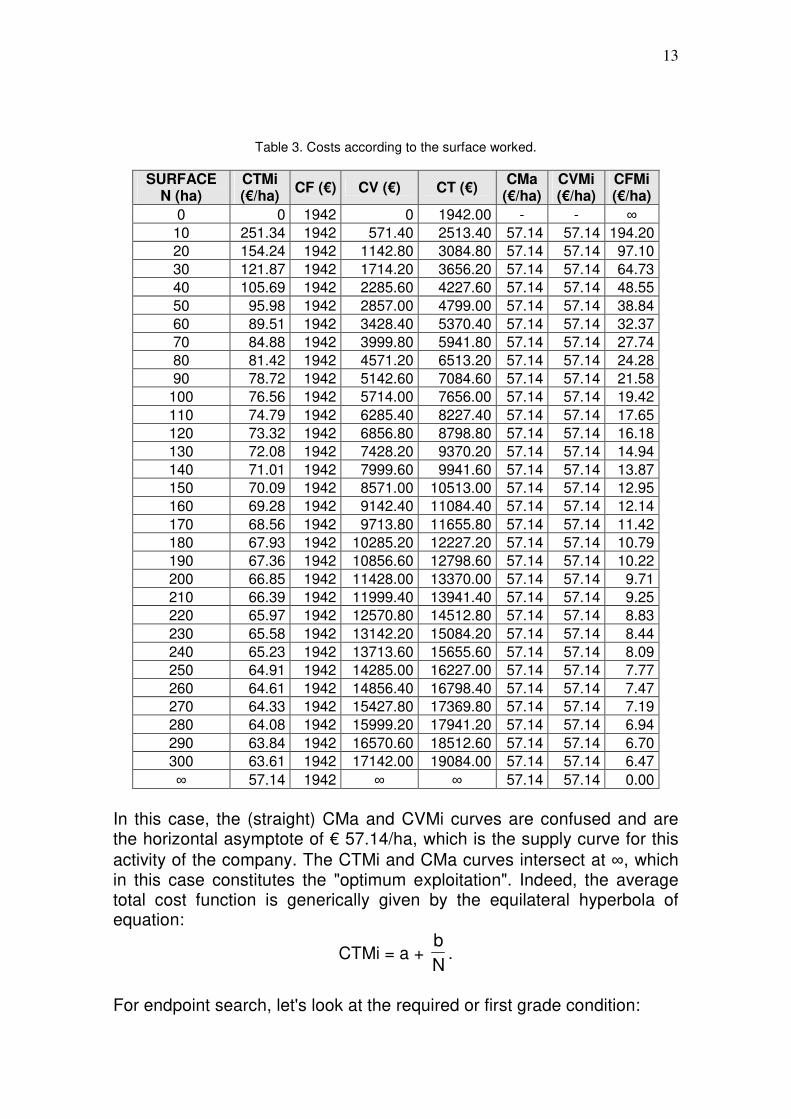
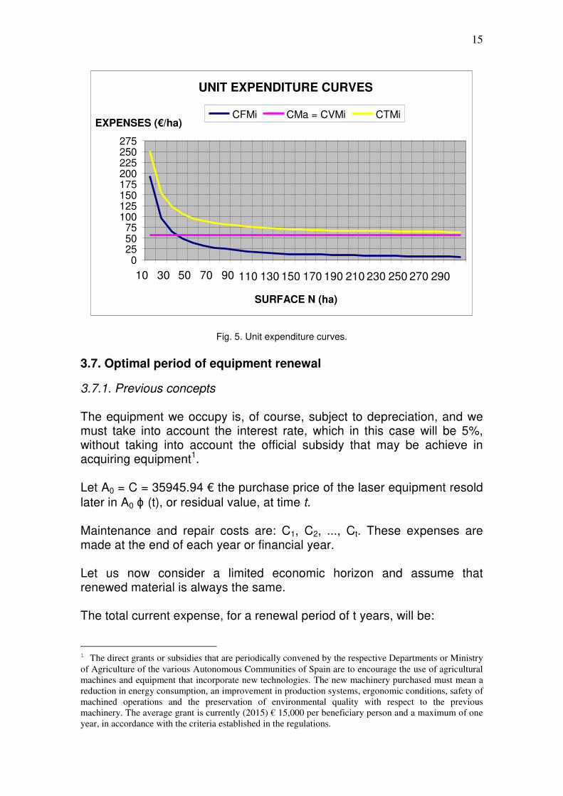
horizontal line, since these costs do not vary with the surface production level N (ha). The vertical distance between the total cost and the fixed cost curve for each level of production obviously represents the variable costs. With respect to the following figure the marginal cost (CMa) is defined as the increase in the total cost needed to produce an additional unit of surface and the shape of the corresponding curve has its origin in the marginal product curve of work. The average or unit costs are per unit of production (leveled and refined ha). The CTMi mean total cost and CVMi mean variable cost curves in this figure are at surface infinity. The relationship between the CMa and CTMi and CVMi curves reflects the general relationship between the marginal and average quantities. The minimum of the total average cost, which coincides with the marginal cost, is known as the optimum operating value of € 57.14/ha. Generally speaking, if the output of an additional unit decreases the average cost, the marginal cost must be less than the average cost. If the production of an additional unit causes the average costs to rise, the cost of that unit (marginal cost) must be greater than the average cost. Accordingly, the marginal cost curve will cut the average cost curve to a minimum. In our case, the following relationships are presented:
CT = 57.14 × N + 1942 ; CTMi = N
1942N14.57 +×;
CTMi = 57.14 + N
1942; −=
dN
dCTMi2N
1942 < 0 (decreasing function);
CMa = dN
dCT= 57.14 > 0 (CT is an increasing function);
CV = 57.14 × N ; CF = 1942 (CF is an constant function);
CVMi = N
N14.57 ×= 57.14 ; CFMi =
N
1942(decreasing function);
These relationships will give rise to the following general cost chart based on the area worked:
In this case, the (straight) CMa and CVMi curves are confused and are the horizontal asymptote of € 57.14/ha, which is the supply curve for this
activity of the company. The CTMi and CMa curves intersect at ∞, which in this case constitutes the "optimum exploitation". Indeed, the average total cost function is generically given by the equilateral hyperbola of equation:
CTMi = a + N
b.
For endpoint search, let's look at the required or first grade condition:
14
2N
b
dN
dCTMi −= = 0 ⇒ N = ∞ → there is a critical point,
thus it is an absolute or global minimum when N = +∞, that is, at the point
(+∞, a), which in our case is that of rectangular Cartesian coordinates
(+∞, 57.14), as well as a absolute or global maximum when N = 0, that is,
at the point (0, +∞). The corresponding curves are as follows:
Fig. 4. Total expenditure curves.
We will also have the following unit expense curves:
3.7.1. Previous concepts The equipment we occupy is, of course, subject to depreciation, and we must take into account the interest rate, which in this case will be 5%, without taking into account the official subsidy that may be achieve in acquiring equipment1. Let A0 = C = 35945.94 € the purchase price of the laser equipment resold
later in A0 ϕ (t), or residual value, at time t. Maintenance and repair costs are: C1, C2, ..., Ct. These expenses are made at the end of each year or financial year. Let us now consider a limited economic horizon and assume that renewed material is always the same. The total current expense, for a renewal period of t years, will be:
1 The direct grants or subsidies that are periodically convened by the respective Departments or Ministry
of Agriculture of the various Autonomous Communities of Spain are to encourage the use of agricultural
machines and equipment that incorporate new technologies. The new machinery purchased must mean a
reduction in energy consumption, an improvement in production systems, ergonomic conditions, safety of
machined operations and the preservation of environmental quality with respect to the previous
machinery. The average grant is currently (2015) € 15,000 per beneficiary person and a maximum of one
year, in accordance with the criteria established in the regulations.
The renewal period t0, which minimizes the total expense, is as follows:
Γ(t0 -1) > Γ(t0) < Γ(t0 + 1). The following considerations need to be made in this regard (Desbazeille, 1969):
- If the residual or resale price at the end of the period [ϕ(t) = 0] is not taken into account, the material will be renewed when:
....
C...CAC
0
0
0
0 t2
t
t10
1t α++α+αα++α+
>+
- If it is accepted that the maintenance expense varies continuously
over time and that the resale price of the equipment is null, the expression of the updated total cost, for a renewal period of t years, it is written thus:
it
t
0
iu
0e1
1du·e)u(cA)t( −
−
−
+=Γ ∫ ,
where c(u) represents the maintenance expense with: e-it ≈ αt .
The total updated expenditure is minimal for a period t0 such that:
[ ]
+=− ∫
−− 00
t
0
iu
0
it
0 du·e)·u(cAie1)t(c . (1)
3.7.2. Exercise In our case, the entertainment expense c(t) of the laser equipment purchased at an A0 acquisition price varies continuously over time. It will be assumed that the renewed material at the end of each period of use is always the same. The unit of time is the year and the expression of c(t) is:
c(t) = α A0 (1 – e-µt).
17
It is therefore a question of establishing the formula that allows to calculate the optimum period of renewal of the leveling/refining laser equipment with the following numerical application:
α = 1/2 ; µ = 1/5 ; i = interest rate = 5% per year. (It should be noted that we have prudentially increased the interest rate by two points, taking into account the foreseeable evolution in the future. In any case, it can be considered the officially published legal interest rate). Solution 1st. According to the above formula (1) the total updated expenditure is minimal for a t0 such that:
−α+=−−α ∫
−µ−−µ− 000
t
0
iuu
00
itt
0 du·e)·e1(A Ai)e1)(e1(A ,
which can also be written like this:
+µα−
+µα+=−α +µ−−µ−
ie
i1i)1e(e 000 t)i(itt
.
2nd. The above formula takes the following form or configuration:
000 t25.0t05.0t20.0 e21)e1(e 10 −−− −=− .
It will be operated by graphical resolution, drawing point by point the representative curves of the following two functions: f(x) = 10 · e-0.20x (1 – e-0.05x) g(x) = 1 – 2e-0.25x and its cut-off point will be found. In any case, analyzing the two expressions analytically, we obtain:
110 ×=−× ; and by multiplying both members by e0.25x, we
get: 10·e0.05x – e0.25x = 8 ; that is: 10·t – t5 = 8 , having made the change of variable: e0.05x = t t5 = e0.25x
18
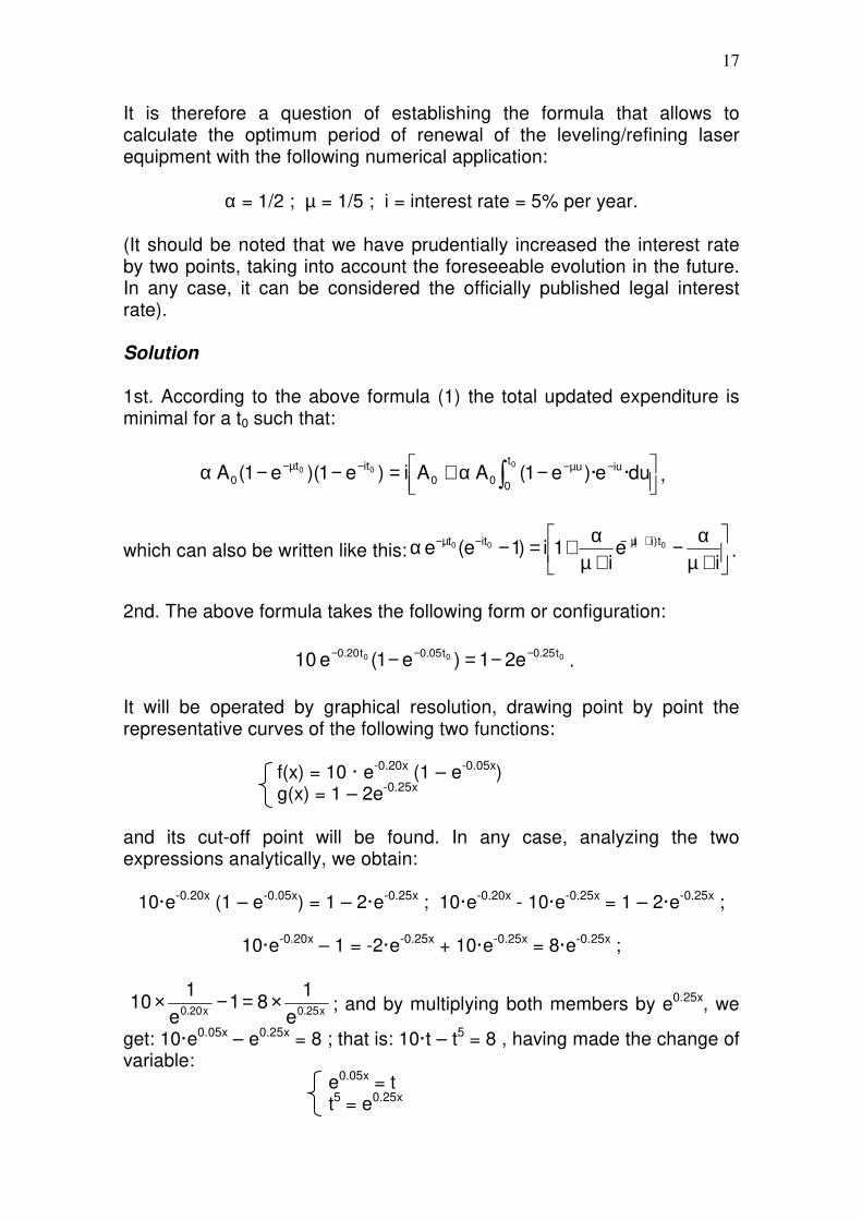
However, the solution of the integer coefficient equation: t5 - 10·t + 8 = 0, offers 5 non-integer roots with convergence problems, so we will opt for their graphical resolution. That is, by giving values to the functions f(x) and g(x), and looking for their intersection point, we obtain the following table (Franquet, 2012):
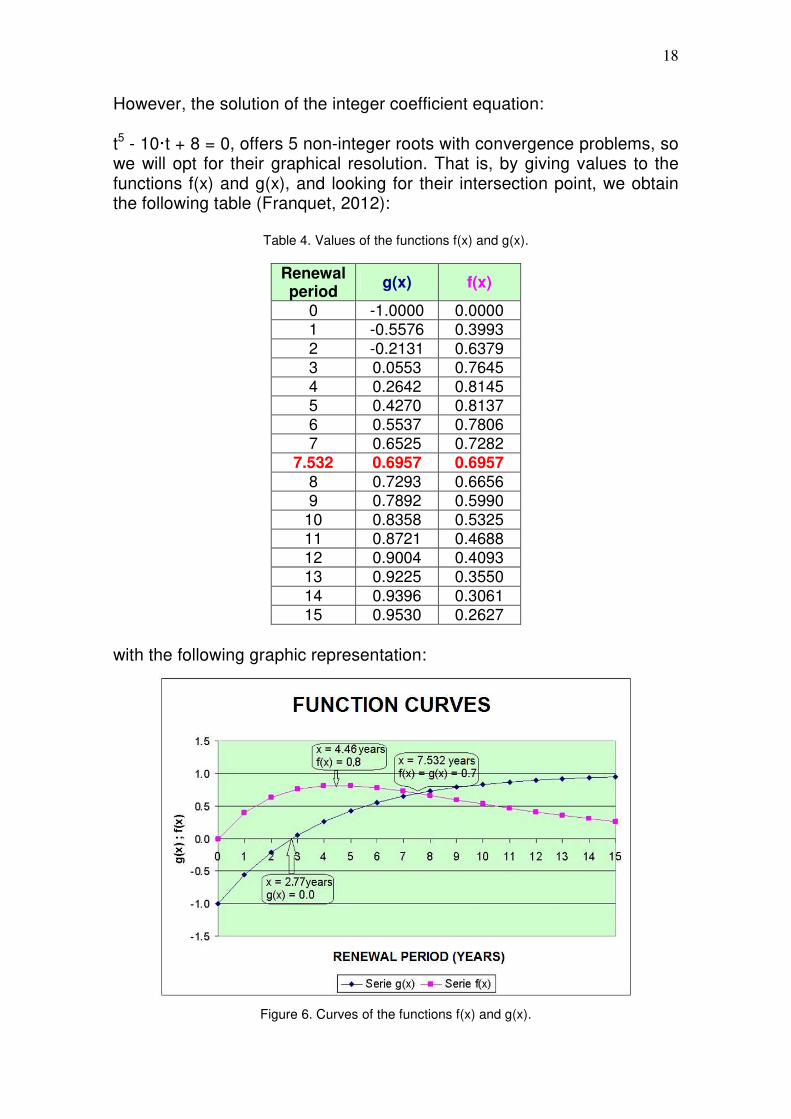
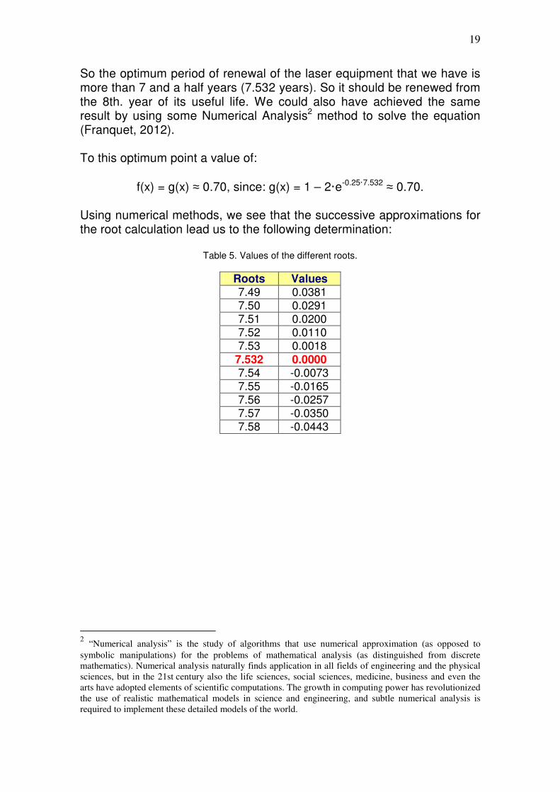
So the optimum period of renewal of the laser equipment that we have is more than 7 and a half years (7.532 years). So it should be renewed from the 8th. year of its useful life. We could also have achieved the same result by using some Numerical Analysis2 method to solve the equation (Franquet, 2012). To this optimum point a value of:
f(x) = g(x) ≈ 0.70, since: g(x) = 1 – 2·e-0.25·7.532 ≈ 0.70. Using numerical methods, we see that the successive approximations for the root calculation lead us to the following determination:
so it is a relative or local maximum at the point of rectangular Cartesian coordinates (4.46, 0.80). 4. CONCLUSIONS In the present study, as an exemplary exercise, the calculation of the profitability threshold of a laser leveling/refining team at a Spanish rice farm, whether individually or in co-operation, through the common use of this modern means of production, while confronting the economic justification of its acquisition with the alternative of renting a similar equipment in the area. It has been concluded that from a surface area of 109 ha (equivalent to 1311 Valencian fanegades) it is already interesting, from a strictly economic point of view, to invest in the purchase of the equipment reviewed. Otherwise, the fact that you do not depend on third-party providers to carry out the work, with the delays, uncertainties and difficulties that this entails, further justifies the convenience of making this investment. It should be borne in mind, in this regard, that according to the latest data from the 20093 agricultural census in Spain, the vast majority of the rice farms in the country have a surface area less than that described, which is why the acquisition and use of the leveling/refining machinery that we are in community, if you do not want to rent the work to third parties. Additionally, the different cost curves and their relationships have been studied and graphically represented from the point of view of Microeconomic Theory, as well as the optimum term of renewal of the team has been determined, following the Operations Research’s own techniques, concluding that, for an equipment of the characteristics studied, its optimum renewal period is around eight years.
3 The information gathering of the 2009 Agricultural Census was carried out between October 2009 and
June 2010. The INE was the responsible body in Spain and in Catalonia it had the collaboration of
Idescat, as well as the Department of Agriculture, Livestock, Fisheries, Food and Natural Environment of
the Generalitat of Catalonia (Spain), according to the corresponding collaboration agreements.
22
BIBLIOGRAPHICAL REFERENCES 1) Desbazeille, G. Ejercicios y problemas de Investigación Operativa. Ed. ICE. Selecciones de Economía de la Empresa. Madrid, 1969. 2) Franquet, J. M. & Querol, A. Nivelación de terrenos por regresión tridimensional. Una aplicación de los métodos estadísticos. Ed. Centro Asociado de la UNED. Cadup-Estudios collection. Tortosa (Spain), 2010. 3) Franquet, J. M. El sector primari a les Terres de l’Ebre. Una aplicació del mètodes quantitatius. Ed. Institut per al Desenvolupament de les Comarques de l’Ebre (IDECE). Generalitat de Catalunya. Tortosa (Spain), 2012.
LIST OF TABLES AND FIGURES: Table 1. Specific consumption according to the speed of revolutions. Table 2. Alternative purchase / rent according to the work surface. Table 3. Costs according to the surface worked. Table 4. Values of the functions f(x) and g(x). Table 5. Values of the different roots. --------- Fig. 1. Agricultural tractor with laser leveling equipment. Fig. 2. Consumption characteristic curve. Fig. 3. Calculation of the profitability threshold of the laser equipment. Fig. 4. Total expenditure curves. Fig. 5. Unit expenditure curves. Fig. 6. Curves of the functions f(x) and g(x). Fig. 7. Approximations for calculating the root of equation.