Annals of Operations Research manuscript No.(will be inserted by the editor)

Leveraging Belief Propagation, Backtrack Search, andStatistics for Model Counting

Lukas Kroc · Ashish Sabharwal · Bart Selman

Received: date / Accepted: date

Abstract We consider the problem of estimating the model count (number of solutions)of Boolean formulas, and present two techniques that compute estimates of these counts,as well as either lower or upper bounds with different trade-offs between efficiency, boundquality, and correctness guarantee. For lower bounds, we use a recent framework for prob-abilistic correctness guarantees, and exploit message passing techniques for marginal prob-ability estimation, namely, variations of the Belief Propagation (BP) algorithm. Our resultssuggest that BP provides useful information even on structured, loopy formulas. For upperbounds, we perform multiple runs of theMiniSat SAT solver with a minor modification, andobtain statistical bounds on the model count based on the observation that the distribution ofa certain quantity of interest is often very close to the normal distribution. Our experimentsdemonstrate that our model counters based on these two ideas,BPCount andMiniCount,can provide very good bounds in time significantly less than alternative approaches.

Keywords Boolean satisfiability· SAT · number of solutions· model counting· BPCount·MiniCount · lower bounds· upper bounds

1 Introduction

The model counting problem for Boolean satisfiability or SAT is the problem of comput-ing the number of solutions or satisfying assignments for a given Boolean formula. Oftenwritten as #SAT, this problem is #P-complete [28] and is widely believed to be significantlyharder than the NP-complete SAT problem, which seeks an answer to whether or not theformula is satisfiable. With the amazing advances in the effectiveness of SAT solvers sincethe early 1990’s, these solvers have come to be commonly used in combinatorial applicationareas such as hardware and software verification, planning, and design automation. Efficient

A preliminary version of this article appeared at the 5th International Conference on Integration of AI andOR Techniques in Constraint Programming for Combinatorial Optimization Problems (CP-AI-OR), Paris,France, 2008 [14].

L. Kroc · A. Sabharwal· B. SelmanDepartment of Computer Science, Cornell University, Ithaca NY 14853-7501, U.S.A.E-mail:{kroc,sabhar,selman}@cs.cornell.edu

2

algorithms for #SAT will further open the doors to a whole new range of applications, mostnotably those involving probabilistic inference [1, 4, 15, 18, 22, 25].

A number of different techniques for model counting have been proposed over the lastfew years. For example,Relsat [2] extends systematic SAT solvers for model countingand uses component analysis for efficiency,Cachet [23, 24] adds caching schemes to thisapproach,c2d [3] converts formulas to the d-DNNF form which yields the model countas a by-product,ApproxCount [30] andSampleCount [10] exploit sampling techniques forestimating the count,MBound [11, 12] relies on the properties of random parity orXOR

constraints to produce estimates with correctness guarantees, and the recently introducedSampleMinisat [9] uses sampling of the backtrack-free search space of systematic SATsolvers. While all of these approaches have their own advantages and strengths, there is stillmuch room for improvement in the overall scalability and effectiveness of model counters.

We propose two new techniques for model counting that leverage the strength of mes-sage passing and systematic algorithms for SAT. The first of these yields probabilistic lowerbounds on the model count, and for the second we introduce a statistical framework forobtaining upper bounds with confidence interval style correctness guarantees.

The first method, which we callBPCount, builds upon a successful approach for modelcounting using local search, calledApproxCount [30]. The idea is to efficiently obtain arough estimate of the “marginals” of each variable: what fraction of solutions have variablexset toTRUE and what fraction havexset toFALSE? If this information is computed accuratelyenough, it is sufficient to recursively count the number of solutions of onlyoneof F |x andF |¬x, and scale the count up appropriately. This technique is extended inSampleCount [10],which adds randomization to this process and provides lower bounds on the model countwith high probability correctness guarantees. For bothApproxCount andSampleCount, truevariable marginals are estimated by obtaining several solution samples using local searchtechniques such asSampleSat [29] and by computing marginals from the samples. In manycases, however, obtaining many near-uniform solution samples can be costly, and one natu-rally asks whether there are more efficient ways of estimating variable marginals.

Interestingly, the problem of computing variable marginals can be formulated as a keyquestion in Bayesian inference, and the Belief Propagation or BP algorithm [cf.19], at leastin principle, provides us with exactly the tool we need. The BP method for SAT involvesrepresenting the problem as a factor graph and passing “messages” back-and-forth betweenvariable and factor nodes until a fixed point is reached. This process is cast as a set of mutu-ally recursive equations which are solved iteratively. From a fixed point of these equations,one can easily compute, in particular, variable marginals.

While this sounds encouraging, there are two immediate challenges in applying the BPframework to model counting: (1) quite often the iterative process for solving the BP equa-tions does not converge to a fixed point, and (2) while BP provably computes exact variablemarginals on formulas whose constraint graph has a tree-like structure (formally definedlater), its marginals can sometimes be substantially off on formulas with a richer interactionstructure. To address the first issue, we use a “message damping” form of BP which hasbetter convergence properties (inspired by a damped version of BP due to Pretti [21]). Forthe second issue, we add “safety checks” to prevent the algorithm from running into a con-tradiction by accidentally eliminating all assignments.1 Somewhat surprisingly, once theserare but fatal mistakes are avoided, it turns out that we can obtain very close estimates andlower bounds for solution counts, suggesting that BP does provide useful information even

1 A tangential approach for handling such fatal mistakes is incorporating BP as a heuristic within back-track search, which our results suggest has clear potential.

3

on highly structured and loopy formulas. To exploit this information even further, we extendthe framework borrowed fromSampleCount with the use of biased random coins duringrandomized value selection for variables.

The model count can, in fact, also be estimated directly from just one fixed point run ofthe BP equations, by computing the value of so-called partition function [32]. In particular,this approach computes the exact model count on tree-like formulas, and appeared to workfairly well on random formulas. However, the count estimated this way is often highly in-accurate on structured loopy formulas.BPCount, as we will see, makes a much more robustuse of the information provided by BP.

The second method, which we callMiniCount, exploits the power of modern Davis-Putnam-Logemann-Loveland or DPLL [5, 6] based SAT solvers, which are extremely goodat finding single solutions to Boolean formulas through backtrack search. (Gogate andDechter [9] have independently proposed the use of DPLL solvers for model counting.) Theproblem of computing upper bounds on the model count has so far eluded an effective solu-tion strategy in part because of an asymmetry that manifests itself in at least two inter-relatedforms: the set of solutions of interestingN variable formulas typically forms a minusculefraction of the full space of 2N variable assignments, and the application of Markov’s in-equality as inSampleCount’s correctness analysis does not yield interesting upper bounds.Note that systematic model counters likeRelsat andCachet can also be easily extended toprovide an upper bound when they time out (2N minus the number of non-solutions encoun-tered during the run), but these bounds are uninteresting because of the above asymmetry.For instance, if a search space of size 21,000 has been explored for a 10,000 variable formulawith as many as 25,000 solutions, the best possible upper bound one could hope to derive withthis reasoning is 210,000−21,000, which is nearly as far away from the true count of 25,000 asthe trivial upper bound of 210,000; the situation only gets worse when the formula has fewersolutions. To address this issue, we develop a statistical framework which lets us computeupper bounds under certain statistical assumptions, which are independently validated. Tothe best of our knowledge, this is the first effective and scalable method for obtaining goodupper bounds on the model counts of formulas that are beyond the reach of exact modelcounters.

More specifically, we describe how the DPLL-based SAT solverMiniSat [7], with twominor modifications, can be used to estimate the total number of solutions. The numberd ofbranching decisions (not counting unit propagations and failed branches) made byMiniSat

before reaching a solution, is the main quantity of interest: when the choice between settinga variable toTRUE or to FALSE is randomized,2 the numberd is provably not any lower, inexpectation, than log2(model count). This provides a strategy for obtaining upper boundson the model count, only if one could efficiently estimate the expected value,E [d], of thenumber of such branching decisions. A natural way to estimateE [d] is to perform multipleruns of the randomized solver, and compute the average ofd over these runs. However,if the formula has many “easy” solutions (found with a low value ofd) and many “hard”solutions, the limited number of runs one can perform in a reasonable amount of time maybe insufficient to hit many of the “hard” solutions, yielding too low of an estimate forE [d]and thus an incorrect upper bound on the model count.

We show that for many families of formulas,d has a distribution that is very close tothe normal distribution. Under the assumption thatd is normally distributed, when samplingvarious values ofd through multiple runs of the solver, one need not necessarily encounterhigh values ofd in order to correctly estimateE [d] for an upper bound. Instead, one can rely

2 MiniSat by default always branches by setting variables first toFALSE.

4

on statistical tests and conservative computations [e.g.27, 34] to obtain a statistical upperbound onE [d] within any specified confidence interval. This is the approach we take in thiswork for our upper bounds.

We evaluated our two approaches on challenging formulas from several domains. Ourexperiments withBPCount demonstrate a clear gain in efficiency, while providing muchhigher lower bound counts than exact counters (which often run out of time or memory orboth) and a competitive lower bound quality compared toSampleCount. For example, theruntime on several difficult instances from the FPGA routing family with over 10100 so-lutions is reduced from hours or more for both exact counters andSampleCount to just afew minutes withBPCount. Similarly, for random 3CNF instances with around 1020 solu-tions, we see a reduction in computation time from hours and minutes to seconds. In somecases, the lower bound provided byMiniCount is somewhat worse than that provided bySampleCount, but still quite competitive. WithMiniCount, we are able to provide good up-per bounds on the solution counts, often within seconds and within a reasonable distancefrom the true counts (if known) or lower bounds computed independently. These experi-mental results attest to the effectiveness of the two proposed approaches in significantlyextending the reach of solution counters for hard combinatorial problems.

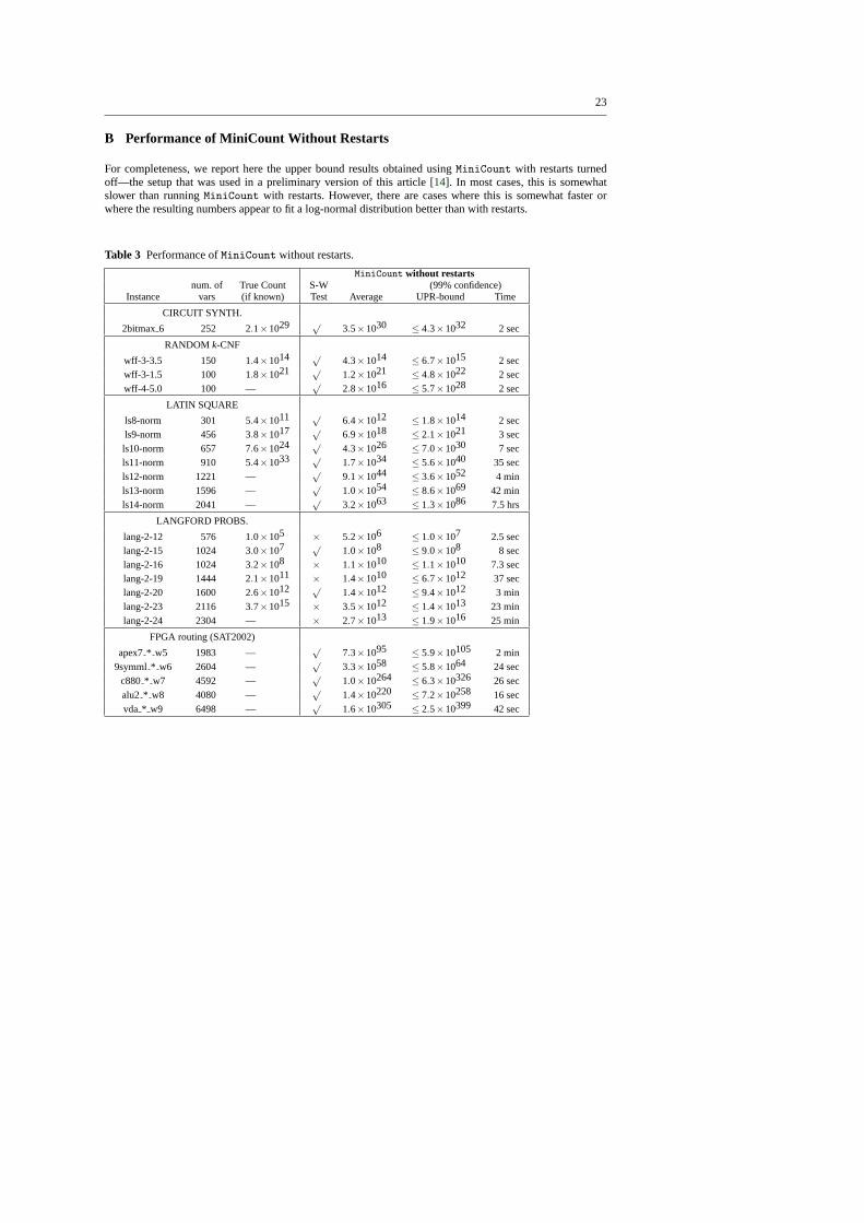
The article is organized as follows. We start in Section2 with preliminaries and notation.Section3 then describes our probabilistic lower bounding approach based on the proposedconvergent form of belief propagation. It first discusses how marginal estimates producedby BP can be used to obtain lower bounds on the model count of a formula by modifying aprevious sampling-based framework, and then suggests two new features to be added to theframework for robustness. Section4 discusses how a backtrack search solver, with appropri-ate randomization and a careful restriction on restarts, can be used to obtain a process thatprovides an upper bound in expectation. It then proposes a statistical technique to estimatethis expected value in a robust manner with statistical confidence guarantees. We presentexperimental results for both of these techniques in Section5 and conclude in Section6.The appendix gives technical details of the convergent form of BP that we propose, as wellas experimental results on the performance of our upper bounding technique when “restarts”are disabled in the underlying backtrack search solver.

2 Notation

A Boolean variablexi is one that assumes a value of either 1 or 0 (TRUE or FALSE, re-spectively). A truth assignment for a set of Boolean variables is a map that assigns eachvariable a value. A Boolean formulaF over a set ofn such variables is a logical expres-sion over these variables, which represents a functionf : {0,1}n → {0,1} determined bywhether or notF evaluates toTRUE under various truth assignments to then variables. Aspecial class of such formulas consists of those in the Conjunctive Normal Form or CNF:F ≡ (l1,1∨ . . .∨ l1,k1)∧ . . .∧ (lm,1∨ . . .∨ lm,km), where each literall l ,k is one of the variablesxi or its negation¬xi . Each conjunct of such a formula is called a clause. We will be workingwith CNF formulas throughout this article.

The constraint graphof a CNF formulaF has variables ofF as vertices and an edgebetween two vertices if both of the corresponding variables appear together in some clauseof F . When this constraint graph has no cycles (i.e., it is a collection of disjoint trees),F iscalled atree-likeor poly-treeformula. Otherwise,F is said to have aloopystructure.

The problem of finding a truth assignment for whichF evaluates toTRUE is known asthepropositional satisfiabilityproblem, or SAT, and is the canonical NP-complete problem.

5

Such an assignment is called asatisfying assignmentor asolutionfor F . A SAT solverrefersto an algorithm, and often an accompanying implementation, for the satisfiability problem.In this work we are concerned with the problem of counting the number of satisfying as-signments for a given formula, known as thepropositional model countingproblem. Wewill also refer to it as thesolution countingproblem. In terms of worst case complexity, thisproblem is #P-complete [28] and is widely believed to be much harder than SAT itself. Amodel counterrefers to an algorithm, and often an accompanying implementation, for themodel counting problem. The model counter is said to beexactif it is guaranteed to outputprecisely the true model count of the input formula when it terminates. The model counterswe propose in this work are randomized and provide either a lower bound or an upper boundon the true model count, with certain correctness guarantees.

3 Lower Bounds Using BP Marginal Estimates: BPCount

In this section, we develop a method for obtaining a lower bound on the solutioncount of a given formula, using the framework recently used in the SAT model counterSampleCount [10]. The key difference between our approach andSampleCount is that in-stead of relying on solution samples, we use a variant of belief propagation to obtain es-timates of the fraction of solutions in which a variable appears positively. We call this al-gorithm BPCount. After describing the basic method, we will discuss two techniques thatimprove the tightness ofBPCount bounds in practice, namely,biased variable assignmentsandsafety checks. Finally, we will describe our variation of the belief propagation algorithmwhich is key to the performance ofBPCount: a set ofparameterizedbelief update equa-tions which are guaranteed to converge for a small enough value of the parameter. Sincethe precise details of these parameterized iterative equations are somewhat tangential to themain focus of this work (namely, model counting techniques), we will defer many of the BPparameterization details to AppendixA.

We begin by recapitulating the framework ofSampleCount for obtaining lower boundmodel counts with probabilistic correctness guarantees. A variableu will be calledbalancedif it occurs equally often positively and negatively in all solutions of the given formula.In general, themarginal probabilityof u being TRUE in the set of satisfying assignmentsof a formula is the fraction of such assignments whereu = TRUE. Note that computing themarginals of each variable, and in particular identifying balanced or near-balanced variables,is quite non-trivial. The model counting approaches we describe attempt to estimate suchmarginals using indirect techniques such as solution sampling or iterative message passing.

Given a formulaF and parameterst,z∈ Z+ andα > 0, SampleCount performst itera-tions, keeping track of the minimum count obtained over these iterations. In each iteration,it samplesz solutions of (potentially simplified)F , identifies the most balanced variableu,uniformly randomly setsu to TRUE or FALSE, simplifiesF by performing any possible unitpropagations, and repeats the process. The repetition ends whenF is reduced to a size smallenough to be feasible for exact model counters such asRelsat [2], Cachet [23], or c2d [3];we will useCachet in the rest of the discussion, as it is the exact model counter we usedin our experiments. At this point, lets denote the number of variables randomly set in thisiteration before handing the formula toCachet, and letM′ be the model count of the resid-ual formula returned byCachet. The count for this iteration is computed to be 2s−α ×M′

(whereα is a “slack” factor pertaining to our probabilistic confidence in the correctness ofthe bound). Here 2s can be seen as scaling up the residual count by a factor of 2 for everyuniform random decision we made when fixing variables. After thet iterations are over, the

6

minimum of the counts over all iterations is reported as the lower bound for the model countof F , and the correctness confidence attached to this lower bound is 1−2−αt . This meansthat the reported count is a correct lower bound on the model count ofF with probability atleast 1−2−αt .

The performance ofSampleCount is enhanced by also considering balanced variablepairs (v,w), where the balance is measured as the difference in the fractions of all solutionsin which v andw appear with the same value vs. with different values. When a pair is morebalanced than any single literal, the pair is used instead for simplifying the formula. In thiscase, we replacew with v or¬v uniformly at random. For ease of illustration, we will focushere only on identifying and randomly setting balanced or near-balanced variables, and notvariable pairs. We note that our implementation of BPCount does support variable pairs.

The key observation inSampleCount is that when the formula is simplified by repeat-edly assigning a positive or negative polarity (i.e.,TRUE or FALSE values, respectively) tovariables, the expected value of the count in each iteration, 2s×M′ (ignoring the slack fac-tor α), is exactly the true model count ofF , from which lower bound guarantees follow.We refer the reader to Gomes et al. [10] for details. Informally, we can think of what hap-pens when the first such balanced variable, sayu, is set uniformly at random. Letp∈ [0,1].SupposeF hasM solutions,F |u has pM solutions, andF |¬u has(1− p)M solutions. Ofcourse, when settingu uniformly at random, we don’t know the actual value ofp. Nonethe-less, with probability a half, we will recursively count the search space withpM solutionsand scale it up by a factor of 2, giving a net count ofpM×2. Similarly, with probability ahalf, we will recursively get a net count of(1− p)M×2 solutions. On average, this gives(1/2× pM×2)+(1/2× (1− p)M×2) = M solutions.

Observe that the correctness guarantee of this process holds irrespective of how goodor bad the samples are, which determines how successful we are in identifying a balancedvariable, i.e., how close isp to 1/2. That said, if balanced variablesare correctly identified,we havep≈ 1/2 in the informal analysis above, which means that for both coin flip outcomeswe recursively search a space containing roughlyM/2 solutions. This reduces thevarianceof this randomized procedure tremendously and is crucial to making the process effectivein practice. Note that with high variance, the minimum count overt iterations is likely to bemuch smaller than the true count; thus high variance leads to lower bounds of poor quality(although still with the same correctness guarantee).

Algorithm BPCount: The idea behindBPCount is to “plug-in” belief propagation methodsin place of solution sampling in theSampleCount framework discussed above,in order toestimate “p” in the intuitive analysis above and, in particular, to help identify balancedvariables. As it turns out, a solution to the BP equations [19] provides exactly what we need:an estimate of the marginals of each variable. This is an alternative to using sampling forthis purpose, and is often orders of magnitude faster.

The heart of the BP algorithm involves solving a set of iterative equations derived specif-ically for a given problem instance (the variables in the system are called “messages”). Theseequations are designed to provide accurate answers if applied to problems with no circulardependencies, such as constraint satisfaction problems with no loops in the correspondingconstraint graph.

One bottleneck, however, is that the basic belief propagation process is iterative anddoes not even converge on most SAT instances of interest. In order to use BP for estimat-ing marginal probabilities and identifying balanced variables, one must either cut off theiterative computation or use a modification that does converge. Unfortunately, some of the

7

known improvements of the belief propagation technique that allow it to converge more of-ten or be used on a wider set of problems, such as Generalized Belief Propagation [31], LoopCorrected Belief Propagation [17], or Expectation Maximization Belief Propagation [13],are not scalable enough for our purposes. The problem of very slow convergence on hardinstances seems to plague also approaches based on other methods for solving BP equa-tions than the simple iteration scheme, such as the convex-concave procedure introducedby Yuille [33]. Finally, in our context, the speed requirement is accentuated by the need touse marginal estimation repeatedly essentially every time a variable is chosen and assigneda value.

We consider a parameterized variant of BP that is guaranteed to converge when thisparameter is small enough, and which imposes no additional computational cost per iterationover standard BP. (A similar but distinct parameterization was proposed by Pretti [21].) Wefound that this “damped” variant of BP provides much more useful information than BPiterations terminated without convergence. We refer to this particular way of damping theBP equations asBPκ , whereκ ≥ 0 is a real valued parameter that controls the extent ofdamping in the iterative equations. The exact details of the corresponding update equationsare not essential for understanding the rest of this article; for completeness, we include theupdate equations for SAT in Figure2 of AppendixA.

The damped equations are analogous to standard BP for SAT,3 differing only in theaddedκ exponent in the iterative update equations. Whenκ = 1, BPκ is identical to regularbelief propagation. On the other hand, whenκ = 0, the equations surely converge in onestep to a unique fixed point and the marginal estimates obtained from this fixed point havea clear probabilistic interpretation in terms of a local property of the variables (we deferformal details of this property to AppendixA; see Proposition1 and the related discussion).Theκ parameter thus allows one to continuously interpolate between two regimes: one withκ = 1 where the equations are identical to standard BP equations and thus provide globalinformation about the solution space if the iterations converge, and another withκ = 0where the iterations surely converge but provide only local information about the solutionspace. In practice,κ is chosen to be roughly the highest value in the range[0,1] that allowsconvergence of the equations within a few seconds or less.

We use the output of BPκ as an estimate of the marginals of the variables inBPCount

(rather than solution samples as inSampleCount). Given this process of obtaining marginalestimates from BP,BPCount works almost exactly likeSampleCount andprovides the samelower bound guarantees.The only difference between the two algorithms is the manner inwhich marginal probabilities of variables is estimated. Formally,

Theorem 1 (Adapted from [10]) Let s denote the number of variables randomly set byan iteration ofBPCount, M′ denote the number of solutions in the final residual formulagiven to an exact model counter, andα > 0 be the slack parameter used. IfBPCount is runwith t ≥ 1 iterations on a formula F, then its output—the minimum of2s−α ×M′ over the titerations—is a correct lower bound on#F with probability at least1−2−αt .

As the exponentially nature of the quantity 1− 2−αt suggests, the correctness confi-dence forBPCount can be easily boosted by increasing the number of iterations,t, (therebyincurring a higher runtime), or by increasing the slack parameter,α, (thereby reporting asomewhat smaller lower bound and thus being conservative), or by a combination of both.In our experiments, we will aim for a correctness confidence of over 99%, by using values

3 See, for example, Figure 4 of [16] with ρ = 0 for a full description of standard BP for SAT.

8

of t andα satisfyingαt ≥ 7. Specifically, most runs will involve 7 iterations andα = 1,while some will involve fewer iterations with a slightly higher value ofα.

3.1 Using Biased Coins

We can improve the performance ofBPCount (and also ofSampleCount) by using biasedvariable assignments. The idea here is that when fixing variables repeatedly in each iteration,the values need not be chosen uniformly. The correctness guarantees still hold even if weuse a biased coin and set the chosen variableu to TRUE with probability q and toFALSE

with probability 1−q, for anyq∈ (0,1). Using earlier notation, this leads us to a solutionspace of sizepM with probabilityq and to a solution space of size(1− p)M with probability1−q. Now, instead of scaling up with a factor of 2 in both cases, we scale up based on thebias of the coin used. Specifically, with probabilityq, we go to one part of the solution spaceand scale it up by 1/q, and similarly for 1− q. The net result is that in expectation, westill get (q× pM/q)+((1−q)× (1− p)M/(1−q)) = M solutions. Further, the variance isminimized whenq is set to equalp; in BPCount, q is set to equal the estimate ofp obtainedusing the BP equations. To see that the resulting variance is minimized this way, note thatwith probabilityq, we get a net count ofpM/q, and with probability(1−q), we get a netcount of(1− p)M/(1−q); these counts balance out to exactlyM in either case whenq= p.Hence, when we have confidence in the correctness of the estimates of variable marginals(i.e., p here), it provably reduces variance to use a biased coin that matches the marginalestimates of the variable to be fixed.

3.2 Safety Checks

One issue that arises when using BP techniques to estimate marginals is that the estimates,in some cases, may be far off from the true marginals. In the worst case, a variableu iden-tified by BP as the most balanced may in fact be a backbone variable forF , i.e., may onlyoccur, say, positively in all solutions toF . Settingu to FALSE based on the outcome of thecorresponding coin flip thus leads one to a part of the search space with no solutions atall, which means that the count for this iteration is zero, making the minimum overt iter-ations zero as well. To remedy this situation, we use safety checks using an off-the-shelfSAT solver (MiniSat [7] or Walksat [26] in our implementation) before fixing the valueof any variable. Note that using a SAT solver as a safety check is a powerful but somewhatexpensive mechanism; fortunately, compared to the problem of counting solutions, the timeto run a SAT solver as a safety check is relatively minor and did not result in any significantslow down in the instances we experimented with. The cost of running a SAT solver to finda solution is also significantly less than the cost other methods such asApproxCount andSampleCount incur when collecting several near-uniform solution samples.

The idea behind the safety check is to simply ensure that there exists at least one solutionboth withu= TRUE and withu= FALSE, beforeflipping a random coin and fixingu to TRUE

or toFALSE. If, say,MiniSat as the safety check solver finds that forcingu to beTRUE makesthe formula unsatisfiable, we can immediately deduceu= FALSE, simplify the formula, andlook for a different balanced variable to continue with; no random coin is flipped in thiscase. If not, we runMiniSat with u forced to beFALSE. If MiniSat finds the formula to beunsatisfiable, we can immediately deduceu = TRUE, simplify the formula, and look for adifferent balanced variable to continue with; again no random coin is flipped in this case. If

9

not, i.e.,MiniSat found solutions both withu set toTRUE andu set toFALSE, thenu is saidto pass the safety check—it is safe to flip a coin and fix the value ofu randomly. This safetycheck preventsBPCount from reaching the undesirable state where there are no remainingsolutions at all in the residual search space.

A slight variant of such a test can also be performed—albeit in a conservative fashion—with an incomplete solver such asWalksat. This works as follows. IfWalksat is unableto find at least one solution both withu beingTRUE andu beingFALSE, we conservativelyassume that it is not safe to flip a coin and fix the value ofu randomly, and instead lookfor another variable for whichWalksat canfind solutions both with valueTRUE and valueFALSE. In the rare case that no such safe variable is found after a few tries, we call this afailed run ofBPCount, and start from the beginning with possibly a higher cutoff forWalksat

or a different safety check solver.Lastly, we note that withSampleCount, the external safety check can be conservatively

replaced by simply avoiding those variables that appear to be backbone variables from theobtained solution samples, i.e., ifu takes valueTRUE in all solution samples at a point, weconservatively assume that it is not safe to assign a random truth value tou.

Remark 1In fact, with the addition of safety checks, we found that the lower bounds onmodel counts obtained for some formulas were surprisingly good even when fake marginalestimates were generated purely at random, i.e., without actually running BP. This can per-haps be explained by the errors introduced at each step somehow canceling out when thevalues of several variables are fixed sequentially. With the use of BP rather than randomlygenerated fake marginals, however, the quality of the lower bounds was significantly im-proved, showing that BP does provide useful information about marginals even for highlyloopy formulas.

4 Upper Bound Estimation Using Backtrack Search: MiniCount

We now describe an approach for estimating an upper bound on the solution count. We usethe reasoning discussed forBPCount, and apply it to a DPLL style backtrack search proce-dure. There is an important distinction between the nature of the bound guarantees presentedhere and earlier: here we will derivestatistical(as opposed to probabilistic) guarantees, andtheir quality may depend on the particular family of formulas in question—in contrast, recallthat the correctness confidence expression 1−2−αt for the lower bound in Theorem1 wasindependent of the nature of the underlying formula or the marginal estimation process. Theapplicability of the method will also be determined by a statistical test, which did succeedin most of our experiments.

For BPCount, we used a backtrack-less search process with a random outcome that, inexpectation, gives the exact number of solutions. The ability to randomly assign values toselected variables was crucial in this process. Here we extend the same line of reasoning toa search processwith backtracking, and argue that the expected value of the outcome is anupper bound on the true count.

We extend the DPLL-based backtrack search SAT solverMiniSat [7] to compute theinformation needed for upper bound estimation.MiniSat is a very efficient SAT solver em-ploying conflict clause learning and other state-of-the-art techniques, and hasone importantfeaturehelpful for our purposes: whenever it chooses a variable to branch on, there is nobuilt-in specialized heuristic to decide which value the variable should assume first. One pos-sibility is to assign valuesTRUE or FALSE randomly with equal probability. SinceMiniSat

10

does not use any information about the variable to determine the most promising polarity,this random assignment in principle does not lowerMiniSat’s power. Note that there areother SAT solvers with this feature, e.g.Rsat [20], and similar results can be obtained forsuch solvers as well.

Algorithm MiniCount: Given a formulaF , runMiniSat, choosing the truth value assign-ment for the variable selected at each choice point uniformly at random betweenTRUE andFALSE (command-line option-polarity-mode=rnd). When a solution is found, output 2d,whered is the “perceived depth”, i.e., the number of choice points on the path to the solu-tion (the final decision level), not counting those choice points where the other branch failedto find a solution (a backtrack point). We rely on the fact that the default implementation ofMiniSat never restarts unless it has backtracked at least once.4

We note that we are implicitly using the fact thatMiniSat, and most SAT solvers avail-able today, assign truth values toall variables of the formula when they declare that a so-lution has been found. In case the underlying SAT solver is designed to detect the fact thatall clauses have been satisfied and to then declare that a solution has been found even with,say,u variables remaining unset, the definition ofd should be modified to include theseuvariables; i.e.,d should beu plus the number of choice points on the path minus the numberof backtrack points on that path.

Note also that for anN variable formula,d can be alternatively defined asN minusthe number of unit propagations on the path to the solution found minus the number ofbacktrack points on that path. This makes it clear thatd is after all tightly related toN, in thesense that if we add a few “don’t care” variables to the formula, the value ofd will increaseappropriately.

We now prove that we can useMiniCount to obtain an upper bound on the true modelcount ofF . SinceMiniCount is a probabilistic algorithm, its output, 2d, on a given formulaF is a random variable. We denote this random variable by #FMiniCount, and use #F to denotethe true number of solutions ofF . The following theorem forms the basis of our upper boundestimation. We note that the theorem provides an essential building block but by itself doesnot fully justify the statistical estimation techniques we will introduce later; they rely onarguments discussed after the theorem.

Theorem 2 For any CNF formula F,E [#FMiniCount]≥ #F.

Proof The expected value is taken across all possible choices made by theMiniCount al-gorithm when run onF , i.e., all its possible computation histories onF . The proof uses thefact that the claimed inequality holds even if all computation histories that incurred at leastone backtrack were modified to output 0 instead of 2d once a solution was found. In otherwords, we will write the desired expected value, by definition, as a sum over all computationhistoriesh and then simply discard a subset of the computation histories—those that involveat least one backtrack—from the sum to obtain a smaller quantity, which will eventually beshown to equal #F exactly.

Once we restrict ourselves to only those computation historiesh that do not involve anybacktracking, these histories correspond one-to-one to the pathsp in the search tree under-lying MiniCount that lead to a solution. Note that there are precisely as many such pathsp as there are satisfying assignments forF . Further, since value choices ofMiniCount at

4 In a preliminary version of this work [14], we did not allow restarts at all. The reasoning given hereextends the earlier argument and permits restarts as long as they happen after at least one backtrack.

11

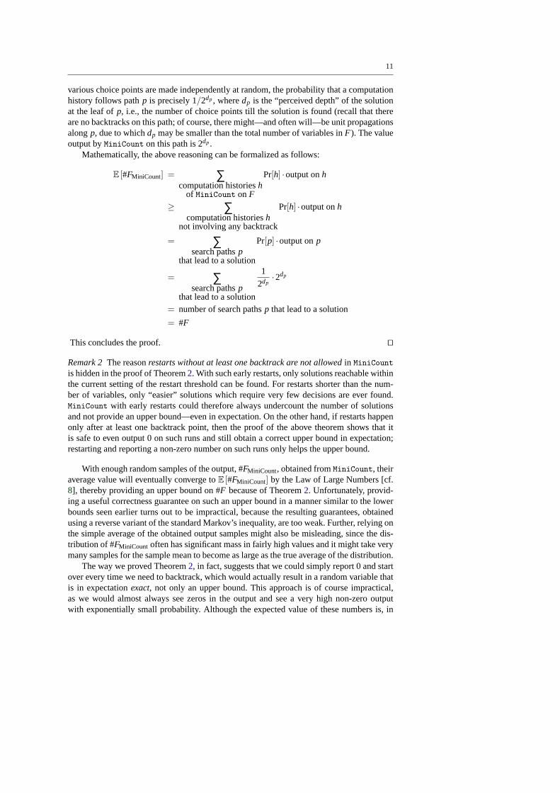
various choice points are made independently at random, the probability that a computationhistory follows pathp is precisely 1/2dp, wheredp is the “perceived depth” of the solutionat the leaf ofp, i.e., the number of choice points till the solution is found (recall that thereare no backtracks on this path; of course, there might—and often will—be unit propagationsalongp, due to whichdp may be smaller than the total number of variables inF). The valueoutput byMiniCount on this path is 2dp.

Mathematically, the above reasoning can be formalized as follows:

E [#FMiniCount] = ∑computation historiesh

of MiniCount onF

Pr[h] ·output onh

≥ ∑computation historiesh

not involving any backtrack

Pr[h] ·output onh

= ∑search pathsp

that lead to a solution

Pr[p] ·output onp

= ∑search pathsp

that lead to a solution

1

2dp·2dp

= number of search pathsp that lead to a solution

= #F

This concludes the proof. ut

Remark 2The reasonrestarts without at least one backtrack are not allowedin MiniCount

is hidden in the proof of Theorem2. With such early restarts, only solutions reachable withinthe current setting of the restart threshold can be found. For restarts shorter than the num-ber of variables, only “easier” solutions which require very few decisions are ever found.MiniCount with early restarts could therefore always undercount the number of solutionsand not provide an upper bound—even in expectation. On the other hand, if restarts happenonly after at least one backtrack point, then the proof of the above theorem shows that itis safe to even output 0 on such runs and still obtain a correct upper bound in expectation;restarting and reporting a non-zero number on such runs only helps the upper bound.

With enough random samples of the output, #FMiniCount, obtained fromMiniCount, theiraverage value will eventually converge toE [#FMiniCount] by the Law of Large Numbers [cf.8], thereby providing an upper bound on #F because of Theorem2. Unfortunately, provid-ing a useful correctness guarantee on such an upper bound in a manner similar to the lowerbounds seen earlier turns out to be impractical, because the resulting guarantees, obtainedusing a reverse variant of the standard Markov’s inequality, are too weak. Further, relying onthe simple average of the obtained output samples might also be misleading, since the dis-tribution of #FMiniCount often has significant mass in fairly high values and it might take verymany samples for the sample mean to become as large as the true average of the distribution.

The way we proved Theorem2, in fact, suggests that we could simply report 0 and startover every time we need to backtrack, which would actually result in a random variable thatis in expectationexact, not only an upper bound. This approach is of course impractical,as we would almost always see zeros in the output and see a very high non-zero outputwith exponentially small probability. Although the expected value of these numbers is, in

12

principle, the true model count ofF , estimating the expected value of the underlying extremezero-heavy ‘bimodal’ distribution through a few random samples is infeasible in practice.We therefore choose to trade off tightness of the reported bound for the ability to obtainvalues that can be argued about, as discussed next.

4.1 Justification for Using Statistical Techniques

As remarked earlier, the proof of Theorem2 by itself does not provide a good justificationfor using statistical estimation techniques to computeE [#FMiniCount]. This is because for thesake of the proving that what we obtain in expectation is an upper bound, we simplified thescenario and showed that it is sufficient to even report 0 solutions and start over wheneverwe need to backtrack. While these 0 outputs are enough to guarantee that we obtain an upperbound in expectation, they are by no means helpful in letting us estimate, in practice, thevalue of this expectation from a few samples of the output value. A bimodal distributionconcentrated on 0 and with exponentially few very large numbers is difficult to estimate theexpected value of. For the technique to be useful in practice, we need a smoother distributionfor which we can use statistical estimation techniques, to be discussed shortly, in order tocompute the expected value in a reasonable manner.

In order to achieve this, we will rely on an important observation:whenMiniCount doesbacktrack, we donot report 0; rather we continue to explore the other side of the “choice”point under consideration and eventually report a non-zero value.Since our strategy willbe to fit a statistical distribution on the output of several samples fromMiniCount, andbecause except for rare occasions all of these samples come after at least one backtrack, itwill be crucial that the non-zero value output byMiniCount when a solution is foundafter abacktrack does have information about the number of solutions ofF . Fortunately, we arguethat this is indeed the case—the value 2d that MiniCount outputs even after at least onebacktrack does contain valuable information about the number of solutions ofF .

To see this, consider a stage in the algorithm that is perceived as a choice point but is infact not a true choice point. Specifically, suppose at this stage, the formula hasM solutionswhenx = TRUE and no solutions whenx = FALSE. With probability 1/2 , MiniCount willsetx to TRUE and in fact estimate an upper bound on 2M from the resulting sub-formula,because it did not discover that it wasn’t really at a “choice” point. This will, of course, stillbe a legal upper bound onM. More importantly, with probability1/2 , MiniCount will setx to FALSE, discover that there are no solutions in this sub-tree, backtrack, setx to TRUE,realize that this is not actually a “choice” point, and recursively estimate an upper bound onM. Thus, even with backtracks, the output ofMiniCount is very closely related to the actualnumber of solutions in the sub-tree at the current stage (unlike in the proof of Theorem2,where it is thought of as being 0), and it is justifiable to deduce an upper bound on #Fby fitting sample outputs ofMiniCount to a statistical distribution. We also note that thenumber of solutions reported after a restart is just like taking another sample of the processwith backtracks, and thus is also closely related to #F.

4.2 Estimating the Upper Bound Using Statistical Methods

In this section, we develop an approach based on statistical analysis of sample outputs thatallows one to estimate the expected value of #FMiniCount, and thus an upper bound withstatistical guarantees, using relatively few samples.

13

Assuming the distribution of #FMiniCount is known, the samples can be used to provide anunbiased estimate of the mean, along with confidence intervals on this estimate. This distri-bution is of course not known and will vary from formula to formula, but it can again be in-ferred from the samples. We observed that for many formulas, the distribution of #FMiniCount

is well approximated by a log-normal distribution. Thus we develop the method under theassumption of log-normality, and include techniques to independently test this assumption.The method has three steps:

1. Generatem independent samples from #FMiniCount by runningMiniCount m times on thesame formula.

2. Test whether the samples come from a log-normal distribution (or a distribution suffi-ciently similar).

3. Estimate the true expected value of #FMiniCount from them samples, and calculate the(1−α) confidence interval for it using the assumption that the underlying distributionis log-normal. We set the confidence levelα to 0.01 (equivalent to a 99% correctnessconfidence as before for the lower bounds), and denote the upper bound of the resultingconfidence interval bycmax.

This process, some of whose details will be discussed shortly, yields an upper boundcmax along with thestatistical guaranteethatcmax≥ E [#FMiniCount], and thuscmax≥ #F byTheorem2:

Pr[cmax≥ #F ] ≥ 1−α (1)

The caveat in this statement (and, in fact, the main difference from the similar statementfor the lower bounds forBPCount given earlier) is that this statement is true only if ourassumption of log-normality of the outputs of single runs of MiniCount on the given formulaholds.

4.2.1 Testing for Log-Normality

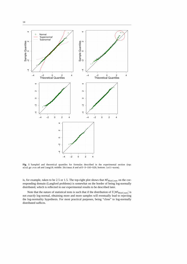
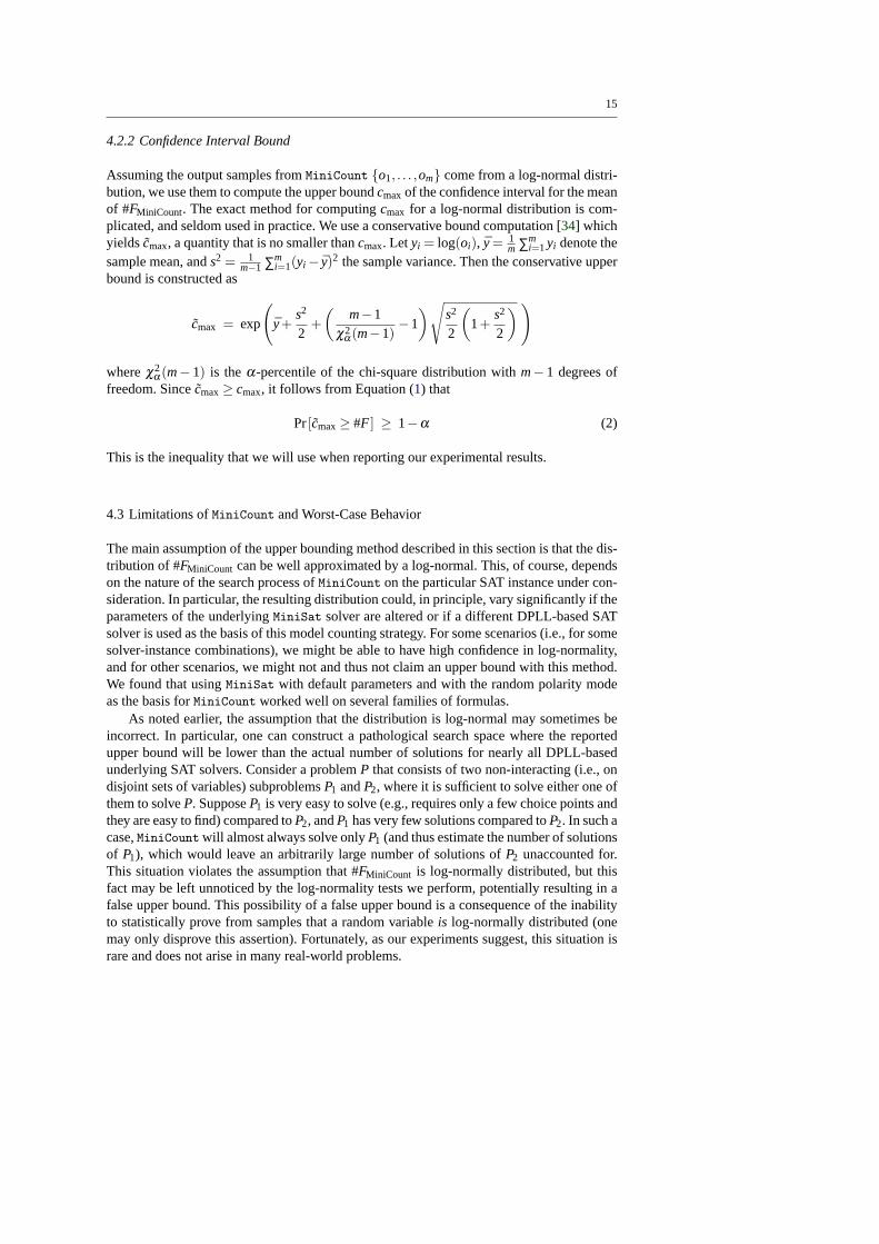
By definition, a random variableX has a log-normal distribution if the random variableY =logX has a normal distribution. Thus a test for whetherY is normally distributed can be used,and we use the Shapiro-Wilk test [cf.27] for this purpose. In our case,Y = log(#FMiniCount)and if the computed p-value of the test is below the confidence levelα = 0.05, we concludethat our samples donotcome from a log-normal distribution; otherwise we assume that theydo. If the test fails, then there is sufficient evidence that the underlying distribution is notlog-normal, and the confidence interval analysis to be described shortly will not provide anystatistical guarantees. Note that non-failure of the test does not mean that the samplesareac-tually log-normally distributed, but inspecting the Quantile-Quantile plots (QQ-plots) oftensupports the hypothesis that they are. QQ-plots compare sampled quantiles with theoreticalquantiles of the desired distribution: the more the sample points align on the diagonal line,the more likely it is that the data came from the desired distribution. See Figure1 for someexamples of QQ-plots.

We found that a surprising number of formulas had log2(#FMiniCount) very close to beingnormally distributed. Figure1 shows normalized QQ-plots fordMiniCount = log2(#FMiniCount)obtained from 100 to 1000 runs ofMiniCount on various families of formulas (discussed inthe experimental section). The top-left QQ-plot shows the best fit of normalizeddMiniCount

(obtained by subtracting the average and dividing by the standard deviation) to the normaldistribution:(normalizeddMiniCount = d)∼ 1√

2πe−d2/2. The ‘supernormal’ and ‘subnormal’

lines show that the fit is much worse when the exponent ofd in the expressione−d2/2 above

14

−4 −2 0 2 4

−4−2

02

4

Theoretical Quantiles

Sam

ple

Qua

ntile

s

Normal’Supernormal’’Subnormal’

−4 −2 0 2 4

−4−2

02

4

Theoretical QuantilesSa

mpl

e Q

uant

iles

−4 −2 0 2 4

−4−2

02

4

−4 −2 0 2 4

−4−2

02

4

−4 −2 0 2 4

−4−2

02

4

Fig. 1 Sampled and theoretical quantiles for formulas described in the experimental section (top:alu2 gr rcs w8 andlang19; middle:2bitmax 6 andwff-3-150-525; bottom:ls11-norm).

is, for example, taken to be 2.5 or 1.5. The top-right plot shows that #FMiniCount on the cor-responding domain (Langford problems) is somewhat on the border of being log-normallydistributed, which is reflected in our experimental results to be described later.

Note that the nature of statistical tests is such that if the distribution ofE [#FMiniCount] isnot exactlylog-normal, obtaining more and more samples will eventually lead to rejectingthe log-normality hypothesis. For most practical purposes, being “close” to log-normallydistributed suffices.

15

4.2.2 Confidence Interval Bound

Assuming the output samples fromMiniCount {o1, . . . ,om} come from a log-normal distri-bution, we use them to compute the upper boundcmax of the confidence interval for the meanof #FMiniCount. The exact method for computingcmax for a log-normal distribution is com-plicated, and seldom used in practice. We use a conservative bound computation [34] whichyieldscmax, a quantity that is no smaller thancmax. Let yi = log(oi), y= 1

m ∑mi=1 yi denote the

sample mean, ands2 = 1m−1 ∑m

i=1(yi − y)2 the sample variance. Then the conservative upperbound is constructed as

cmax = exp

(y+

s2

2+(

m−1χ2

α(m−1)−1

)√s2

2

(1+

s2

2

) )

whereχ2α(m− 1) is theα-percentile of the chi-square distribution withm− 1 degrees of

freedom. Since ˜cmax≥ cmax, it follows from Equation (1) that

Pr[cmax≥ #F ] ≥ 1−α (2)

This is the inequality that we will use when reporting our experimental results.

4.3 Limitations ofMiniCount and Worst-Case Behavior

The main assumption of the upper bounding method described in this section is that the dis-tribution of #FMiniCount can be well approximated by a log-normal. This, of course, dependson the nature of the search process ofMiniCount on the particular SAT instance under con-sideration. In particular, the resulting distribution could, in principle, vary significantly if theparameters of the underlyingMiniSat solver are altered or if a different DPLL-based SATsolver is used as the basis of this model counting strategy. For some scenarios (i.e., for somesolver-instance combinations), we might be able to have high confidence in log-normality,and for other scenarios, we might not and thus not claim an upper bound with this method.We found that usingMiniSat with default parameters and with the random polarity modeas the basis forMiniCount worked well on several families of formulas.

As noted earlier, the assumption that the distribution is log-normal may sometimes beincorrect. In particular, one can construct a pathological search space where the reportedupper bound will be lower than the actual number of solutions for nearly all DPLL-basedunderlying SAT solvers. Consider a problemP that consists of two non-interacting (i.e., ondisjoint sets of variables) subproblemsP1 andP2, where it is sufficient to solve either one ofthem to solveP. SupposeP1 is very easy to solve (e.g., requires only a few choice points andthey are easy to find) compared toP2, andP1 has very few solutions compared toP2. In such acase,MiniCount will almost always solve onlyP1 (and thus estimate the number of solutionsof P1), which would leave an arbitrarily large number of solutions ofP2 unaccounted for.This situation violates the assumption that #FMiniCount is log-normally distributed, but thisfact may be left unnoticed by the log-normality tests we perform, potentially resulting in afalse upper bound. This possibility of a false upper bound is a consequence of the inabilityto statistically prove from samples that a random variableis log-normally distributed (onemay only disprove this assertion). Fortunately, as our experiments suggest, this situation israre and does not arise in many real-world problems.

16

5 Experimental Results

We conducted experiments withBPCount as well asMiniCount,5 with the primary focuson comparing the results to exact counters and the recentSampleCount algorithm providingprobabilistically guaranteed lower bounds. We used a cluster of 3.8 GHz Intel Xeon com-puters running Linux 2.6.9-22.ELsmp. The time limit was set to 12 hours and the memorylimit to 2 GB.

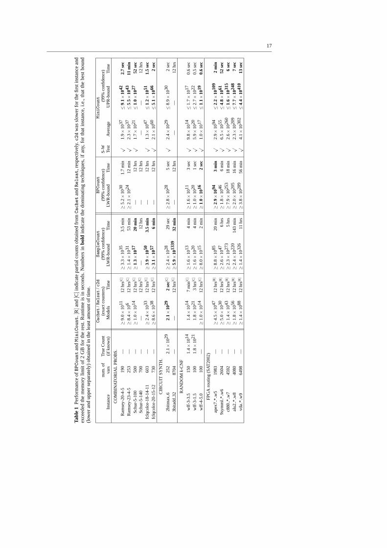
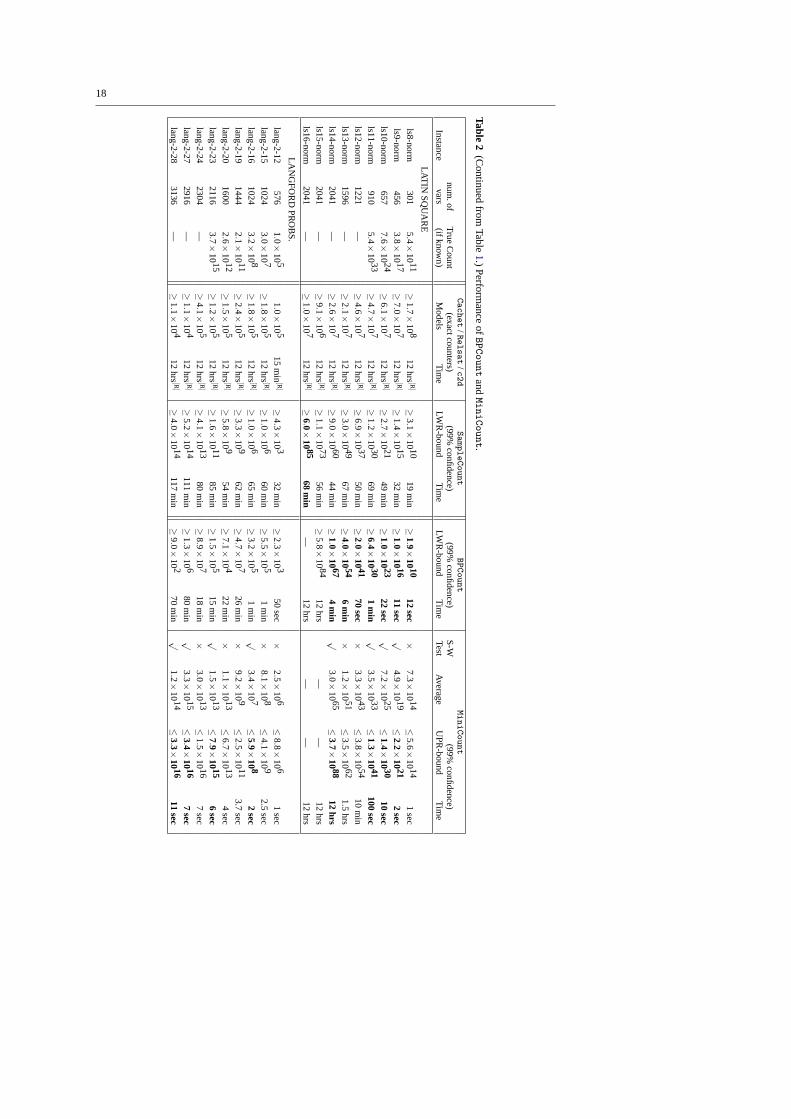
We consider problems from five different domains, many of which have previously beenused as benchmarks for evaluating model counting techniques: circuit synthesis, random k-CNF, Latin square construction, Langford problems, and FPGA routing instances from theSAT 2002 competition. The results are summarized in Tables1 and2.

The columns show the performance ofBPCount (version 1.2LES, based onSampleCount version 1.2L but adding external BP-based marginals and safety checks, us-ing Cachet version 1.2 once the instance under consideration is sufficiently simplified) andMiniCount (based onMiniSat version 2.0), compared against the exact solution countersRelsat (version 2.00),Cachet (version 1.2), andc2d (version 2.20)6, and the lower bound-ing solution counterSampleCount (version 1.2L, usingCachet version 1.2 once the instanceis sufficiently simplified). The tables show the reported bounds on the model counts and thecorresponding runtime in seconds.

For BPCount, the damping parameter setting (i.e., theκ value) we use for the dampedBP marginal estimator is 0.8, 0.9, 0.9, 0.5, and either 0.1 or 0.2, for the five domains, re-spectively. This parameter is chosen (with a quick manual search) as high as possible whilestill allowing BPκ iterations to converge to a fixed point in a few seconds or less. The exactcounterCachet is called when the formula is sufficiently simplified, which is when 50 to500 variables remain, depending on the domain. The lower bounds on the model count arereported with 99% correctness confidence.

Tables1 and 2 show that a significant improvement in efficiency is achieved whenthe BP marginal estimation is used throughBPCount, rather than solution sampling as inSampleCount (also run with 99% correctness confidence). For the smaller formulas consid-ered, the lower bounds reported byBPCount border the true model counts. For the largerones that could only be counted partially by exact counters in 12 hours,BPCount gave lowerbound counts that are very competitive with those reported bySampleCount, while the run-ning time ofBPCount is, in general, an order of magnitude lower than that ofSampleCount,often just a few seconds.

For MiniCount, we obtainm = 100 samples of the estimated count for each formula,and use these to estimate the upper bound statistically using the steps described earlier.The test for log-normality of the sample counts is done with a rejection level of 0.05, thatis, if the Shapiro-Wilk test reports a p-value below 0.05, we conclude the samples donotcome from a log-normal distribution, in which case no upper bound guarantees are provided(MiniCount is “unsuccessful”). When the test passed, the upper bound itself was computedwith a confidence level of 99% using the computation discussion in Section4.2.2. The re-sults are summarized in the last set of columns in Tables1 and2. We report whether the

5 As stated earlier, we allow restarts inMiniCount after at least one backtrack has occurred, unlike thepreliminary version of this work [14] where we reported results without restarts. Although the results in thetwo scenarios are sometimes fairly close, we believe allowing restarts will be effective and even indispensableon harder problem instances. We thus report here numbers only with restarts. For completeness, the numbersfor MiniCount without restarts are reported in Table3 of AppendixB.

6 We report counts obtained from the best of the three exact model counters for each instance; for all butthe first instance,c2d exceeded the memory limit.

17

Tabl

e1

Per

form

ance

ofBPCount

andMiniCount.[

R]a

nd[C

]ind

icat

epa

rtia

lcou

nts

obta

ined

fromCachet

andRelsat,r

espe

ctiv

ely.c2d

was

slow

erfo

rth

efir

stin

stan

cean

dex

ceed

edth

em

emor

ylim

itof

2G

Bfo

rth

ere

st.

Run

time

isin

seco

nds.

Num

bers

inbo

ldin

dica

teth

edo

min

atin

gte

chni

ques

,if

any,

for

that

inst

ance

,i.e

.,th

atth

ebe

stbo

und

(low

eran

dup

per

sepa

rate

ly)

obta

ined

inth

ele

asta

mou

ntof

time.

Cachet

/Relsat

/c2d

SampleCount

BPCount

MiniCount

num

.of

Tru

eC

ount

(exa

ctco

unte

rs)

(99%

confi

denc

e)(9

9%co

nfide

nce)

S-W

(99%

confi

denc

e)In

stan

ceva

rs(if

know

n)M

odel

sT

ime

LWR

-bou

ndT

ime

LWR

-bou

ndT

ime

Test

Ave

rage

UP

R-b

ound

Tim

e

CO

MB

INAT

OR

IAL

PR

OB

S.

Ram

sey-

20-4

-519

0—

≥9.

0×

1011

12hr

s[C]

≥3.

3×

1035

3.5

min

≥5.

2×

1030

1.7

min

√1.

9×

1037

≤9.

1×

1042

2.7

sec

Ram

sey-

23-4

-525

3—

≥8.

4×

106

12hr

s[C]

≥1.

4×

1031

53m

in≥

2.1×

1024

12m

in√

2.3×

1037

≤5.

5×

1043

11m

inS

chur

-5-1

0050

0—

≥1.

0×

1014

12hr

s[C]

≥1.

3×

1017

20m

in—

12hr

s√

1.7×

1021

≤1.

0×

1027

52se

cS

chur

-5-1

4070

0—

—12

hrs[C

]—

12hr

s—

12hr

s—

—12

hrs

fclq

colo

r-18

-14-

1160

3—

≥2.

4×

1033

12hr

s[C]

≥3.

9×

1050

3.5

min

—12

hrs

√1.

3×

1047

≤1.

2×

1051

1.5

sec

fclq

colo

r-20

-15-

1273

0—

≥8.

6×

1038

12hr

s[C]

≥3.

1×

1057

6m

in—

12hr

s√

2.1×

1060

≤5.

1×

1066

2se

c

CIR

CU

ITS

YN

TH

.

2bitm

ax6

252

2.1×

1029

2.1×

1029

2se

c[C]

≥2.

4×

1028

29se

c≥

2.8×

1028

5se

c√

2.4×

1029

≤8.

9×

1030

2se

c3b

itadd

3287

04—

—12

hrs[C

]≥

5.9×

1013

3932

min

—12

hrs

——

12hr

s

RA

ND

OM

k-C

NF

wff-

3-3.

515

01.4×

1014

1.4×

1014

7m

in[C

]≥

1.6×

1013

4m

in≥

1.6×

1011

3se

c√

9.8×

1014

≤1.

7×

1017

0.6

sec

wff-

3-1.

510

01.8×

1021

1.8×

1021

3hr

s[C]

≥1.

6×

1020

4m

in≥

1.0×

1020

1se

c√

5.9×

1020

≤2.

7×

1022

0.5

sec

wff-

4-5.

010

0—

≥1.

0×

1014

12hr

s[C]

≥8.

0×

1015

2m

in≥

1.0×

1016

2se

c√

1.0×

1017

≤1.

1×

1019

0.6

sec

FP

GA

rout

ing

(SAT

2002

)

apex

7*

w5

1983

—≥

4.5×

1047

12hr

s[R]

≥8.

8×

1085

20m

in≥

2.9×

1094

3m

in√

2.9×

1094

≤2.

2×

1010

92

min

9sym

ml*

w6

2604

—≥

5.0×

1030

12hr

s[R]

≥2.

6×

1047

6hr

s≥

1.8×

1046

6m

in√

6.5×

1055

≤4.

8×

1061

52se

cc8

80*

w7

4592

—≥

1.4×

1043

12hr

s[R]

≥2.

3×

1027

35

hrs

≥7.

9×

1025

318

min

√2.

6×

1026

0≤

1.6×

1031

56

sec

alu2

*w

840

80—

≥1.

8×

1056

12hr

s[R]

≥2.

4×

1022

014

3m

in≥

2.0×

1020

516

min

√2.

3×

1020

9≤

7.7×

1024

87

sec

vda

*w

964

98—

≥1.

4×

1088

12hr

s[R]

≥1.

4×

1032

611

hrs

≥3.

8×

1028

956

min

√4.

1×

1030

2≤

4.4×

1041

013

sec

18

Table2

(Continued

fromTable1.)

Perform

anceofBP

Count

andMiniCount.

Cachet

/Relsat

/c2d

SampleCount

BPCount

MiniCount

num.of

True

Count

(exactcounters)(99%

confidence)(99%

confidence)S

-W(99%

confidence)Instance

vars(ifknow

n)M

odelsT

ime

LWR

-boundT

ime

LWR

-boundT

ime

TestA

verageU

PR

-boundT

ime

LATIN

SQ

UA

RE

ls8-norm301

5.4×10 11

≥1.7×

10 812

hrs [R]

≥3.1×

10 1019

min

≥1.9×

10 1012

sec×

7.3×10 14

≤5.6×

10 141

secls9-norm

4563.8×

10 17≥

7.0×

10 712

hrs [R]

≥1.4×

10 1532

min

≥1.0×

10 1611

sec√

4.9×10 19

≤2.2×

10 212

secls10-norm

6577.6×

10 24≥

6.1×

10 712

hrs [R]

≥2.7×

10 2149

min

≥1.0×

10 2322

sec√

7.2×10 25

≤1.4×

10 3010

secls11-norm

9105.4×

10 33≥

4.7×

10 712

hrs [R]

≥1.2×

10 3069

min

≥6.4×

10 301

min

√3.5×

10 33≤

1.3×10 41

100sec

ls12-norm1221

—≥

4.6×

10 712

hrs [R]

≥6.9×

10 3750

min

≥2.0×

10 4170

sec×

3.3×10 43

≤3.8×

10 5410

min

ls13-norm1596

—≥

2.1×

10 712

hrs [R]

≥3.0×

10 4967

min

≥4.0×

10 546

min

×1.2×

10 51≤

3.5×10 62

1.5hrs

ls14-norm2041

—≥

2.6×

10 712

hrs [R]

≥9.0×

10 6044

min

≥1.0×

10 674

min

√3.0×

10 65≤

3.7×10 88

12hrs

ls15-norm2041

—≥

9.1×

10 612

hrs [R]

≥1.1×

10 7356

min

≥5.8×

10 8412

hrs—

—12

hrsls16-norm

2041—

≥1.0×

10 712

hrs [R]

≥6.0×

10 8568

min

—12

hrs—

—12

hrs

LAN

GF

OR

DP

RO

BS

.

lang-2-12576

1.0×10 5

1.0×10 5

15m

in [R]

≥4.3×

10 332

min

≥2.3×

10 350

sec×

2.5×10 6

≤8.8×

10 61

seclang-2-15

10243.0×

10 7≥

1.8×

10 512

hrs [R]

≥1.0×

10 660

min

≥5.5×

10 51

min

×8.1×

10 8≤

4.1×10 9

2.5sec

lang-2-161024

3.2×10 8

≥1.8×

10 512

hrs [R]

≥1.0×

10 665

min

≥3.2×

10 51

min

√3.4×

10 7≤

5.9×10 8

2sec

lang-2-191444

2.1×10 11

≥2.4×

10 512

hrs [R]

≥3.3×

10 962

min

≥4.7×

10 726

min

×9.2×

10 9≤

2.5×10 11

3.7sec

lang-2-201600

2.6×10 12

≥1.5×

10 512

hrs [R]

≥5.8×

10 954

min

≥7.1×

10 422

min

×1.1×

10 13≤

6.7×10 13

4sec

lang-2-232116

3.7×10 15

≥1.2×

10 512

hrs [R]

≥1.6×

10 1185

min

≥1.5×

10 515

min

√1.5×

10 13≤

7.9×10 15

6sec

lang-2-242304

—≥

4.1×

10 512

hrs [R]

≥4.1×

10 1380

min

≥8.9×

10 718

min

×3.0×

10 13≤

1.5×10 16

7sec

lang-2-272916

—≥

1.1×

10 412

hrs [R]

≥5.2×

10 14111

min

≥1.3×

10 680

min

√3.3×

10 15≤

3.4×10 16

7sec

lang-2-283136

—≥

1.1×

10 412

hrs [R]

≥4.0×

10 14117

min

≥9.0×

10 270

min

√1.2×

10 14≤

3.3×10 16

11sec

19

log-normality test passed, the average of the counts obtained over the 100 runs, the value ofthe statistical upper boundcmax, and the total time for the 100 runs.

Tables1 and2 show that the upper bounds are often obtained within seconds or minutes,and are correct for all instances where the estimation method was successful (i.e., the log-normality test passed) and true counts or lower bounds are known. In fact, the upper boundsfor these formulas (exceptlang-2-23) are correct w.r.t. the best known lower bounds andtrue counts even for those instances where the log-normality test failed and a statisticalguarantee cannot be provided. The Langford problem family seems to be at the boundaryof applicability of theMiniCount approach, as indicated by the alternating successes andfailures of the test in this case. The approach is particularly successful on industrial problems(circuit synthesis, FPGA routing), where upper bounds are computed within seconds.

Our results also demonstrate that a simple average of the 100 runs can provide a verygood approximation to the number of solutions. However, simple averaging can sometimeslead to an incorrect upper bound, as seen inwff-3-1.5, ls13-norm, alu2 gr rcs w8, andvda gr rcs w9, where the simple average is below the true count or a lower bound obtainedindependently. This justifies our statistical framework as an effective strategy for obtainingmore robust upper bounds.

We end this section with the observation that while the lower and upper bounds providedby BPCount andMiniCount, respectively, are in general of very good quality, there is stilla gap in the exponent. From the results for the cases where the true solution count for theinstance is known, we can see that either of these bounds can be closer to the true count thanthe other. For example, the lower bound reported byBPCount is tigher than the upper boundreported byMiniCount in the case of the Latin Square construction problem, the oppositeholds for the Langford problem, and the true count lies roughly in the middle (in log-scale)for the randomly generated problem. This attests to the hardness of the model countingproblem and leaves open room for further improvement in techniques for obtaining bothlower bounds and upper bounds on the true count.

6 Conclusion

This work brings together techniques from message passing, DPLL-based SAT solvers, andstatistical estimation in an attempt to solve the challenging model counting problem. Weshow how (a damped form of) BP can help significantly boost solution counters that pro-duce lower bounds with probabilistic correctness guarantees.BPCount is able to providegood quality, competitive lower bounds in a fraction of the time compared to previous,sampling-based methods. We also describe the first effective approach for obtaining goodupper bounds on the solution count. Our framework is general and enables one to turn anystate-of-the-art complete SAT solver into an upper bound counter, with very minimal mod-ifications to the code. OurMiniCount algorithm provably converges to an upper bound onthe solution count as more and more samples are drawn, and a statistical estimate of thisupper bound can be efficiently derived from just a few samples assuming an independentlyverified log-normality condition.MiniCount is shown to be remarkably fast at providinggood upper bounds in practice.

Acknowledgements This work was supported by the Intelligent Information Systems Institute, Cornell Uni-versity (Air Force Office of Scientific Research AFOSR, grant FA9550-04-1-0151), the Defence AdvancedResearch Projects Agency (DARPA, REAL Program, grant FA8750-04-2-0216), and the National ScienceFoundation (NSF IIS award, grant 0514429; NSF Expeditions in Computing award for Computational Sus-tainability, grant 0832782).

20

References

1. F. Bacchus, S. Dalmao, and T. Pitassi. Solving #SAT and Bayesian inference withbacktracking search.Journal of Artificial Intelligence Research, 34:391–442, 2009.

2. R. J. Bayardo Jr. and J. D. Pehoushek. Counting models using connected components.In Proceedings of AAAI-00: 17th National Conference on Artificial Intelligence, pages157–162, Austin, TX, July 2000.

3. A. Darwiche. New advances in compiling CNF into decomposable negation normalform. In Proceedings of ECAI-04: 16th European Conference on Artificial Intelligence,pages 328–332, Valencia, Spain, Aug. 2004.

4. A. Darwiche. The quest for efficient probabilistic inference, July 2005. Invited Talk,IJCAI-05.

5. M. Davis, G. Logemann, and D. Loveland. A machine program for theorem proving.Communications of the ACM, 5:394–397, 1962.

6. M. Davis and H. Putnam. A computing procedure for quantification theory.Communi-cations of the ACM, 7:201–215, 1960.

7. N. Een and N. Sorensson. MiniSat: A SAT solver with conflict-clause minimization.In Proceedings of SAT-05: 8th International Conference on Theory and Applications ofSatisfiability Testing, St. Andrews, U.K., June 2005.

8. W. Feller.An Introduction to Probability Theory and Its Applications, Volume 1. Wiley,3rd edition, 1968.

9. V. Gogate and R. Dechter. Approximate counting by sampling the backtrack-free searchspace. InProceedings of AAAI-07: 22nd Conference on Artificial Intelligence, pages198–203, Vancouver, BC, July 2007.

10. C. P. Gomes, J. Hoffmann, A. Sabharwal, and B. Selman. From sampling to modelcounting. InProceedings of IJCAI-07: 20th International Joint Conference on ArtificialIntelligence, pages 2293–2299, Hyderabad, India, Jan. 2007.

11. C. P. Gomes, A. Sabharwal, and B. Selman. Model counting: A new strategy for obtain-ing good bounds. InProceedings of AAAI-06: 21st Conference on Artificial Intelligence,pages 54–61, Boston, MA, July 2006.

12. C. P. Gomes, W.-J. van Hoeve, A. Sabharwal, and B. Selman. Counting CSP solutionsusing generalized XOR constraints. InProceedings of AAAI-07: 22nd Conference onArtificial Intelligence, pages 204–209, Vancouver, BC, July 2007.

13. E. I. Hsu and S. A. McIlraith. Characterizing propagation methods for boolean satis-fiabilty. In Proceedings of SAT-06: 9th International Conference on Theory and Ap-plications of Satisfiability Testing, volume 4121 ofLecture Notes in Computer Science,pages 325–338, Seattle, WA, Aug. 2006.

14. L. Kroc, A. Sabharwal, and B. Selman. Leveraging belief propagation, backtrack search,and statistics for model counting. InCPAIOR-08: 5th International Conference on Inte-gration of AI and OR Techniques in Constraint Programming, volume 5015 ofLectureNotes in Computer Science, pages 127–141, Paris, France, May 2008.

15. M. L. Littman, S. M. Majercik, and T. Pitassi. Stochastic Boolean satisfiability.Journalof Automated Reasoning, 27(3):251–296, 2001.

16. E. Maneva, E. Mossel, and M. J. Wainwright. A new look at survey propagation and itsgeneralizations.Journal of the ACM, 54(4):17, July 2007.

17. J. M. Mooij, B. Wemmenhove, H. J. Kappen, and T. Rizzo. Loop corrected beliefpropagation. InProceedings of AISTATS-07: 11th International Conference on ArtificialIntelligence and Statistics, San Juan, Puerto Rico, Mar. 2007.

21

18. J. D. Park. MAP complexity results and approximation methods. InProceedings ofUAI-02: 18th Conference on Uncertainty in Artificial Intelligence, pages 388–396, Ed-monton, Canada, Aug. 2002.

19. J. Pearl. Probabilistic Reasoning in Intelligent Systems: Networks of Plausible Infer-ence. Morgan Kaufmann, 1988.

20. K. Pipatsrisawat and A. Darwiche. RSat 1.03: SAT solver description. Technical ReportD–152, Automated Reasoning Group, Computer Science Department, UCLA, 2006.

21. M. Pretti. A message-passing algorithm with damping.Journal of Statistical Mechan-ics, P11008, 2005.

22. D. Roth. On the hardness of approximate reasoning.Artificial Intelligence, 82(1-2):273–302, 1996.

23. T. Sang, F. Bacchus, P. Beame, H. A. Kautz, and T. Pitassi. Combining componentcaching and clause learning for effective model counting. InProceedings of SAT-04:7th International Conference on Theory and Applications of Satisfiability Testing, Van-couver, BC, May 2004.

24. T. Sang, P. Beame, and H. A. Kautz. Heuristics for fast exact model counting. InProceedings of SAT-05: 8th International Conference on Theory and Applications ofSatisfiability Testing, volume 3569 ofLecture Notes in Computer Science, pages 226–240, St. Andrews, U.K., June 2005.

25. T. Sang, P. Beame, and H. A. Kautz. Performing Bayesian inference by weighted modelcounting. InProceedings of AAAI-05: 20th National Conference on Artificial Intelli-gence, pages 475–482, Pittsburgh, PA, July 2005.

26. B. Selman, H. Kautz, and B. Cohen. Local search strategies for satisfiability testing. InD. S. Johnson and M. A. Trick, editors,Cliques, Coloring and Satisfiability: the SecondDIMACS Implementation Challenge, volume 26 ofDIMACS Series in Discrete Math-ematics and Theoretical Computer Science, pages 521–532. American MathematicalSociety, 1996.

27. H. C. Thode.Testing for Normality. CRC, 2002.28. L. G. Valiant. The complexity of computing the permanent.Theoretical Computer

Science, 8:189–201, 1979.29. W. Wei, J. Erenrich, and B. Selman. Towards efficient sampling: Exploiting random

walk strategies. InProceedings of AAAI-04: 19th National Conference on ArtificialIntelligence, pages 670–676, San Jose, CA, July 2004.

30. W. Wei and B. Selman. A new approach to model counting. InProceedings of SAT-05: 8th International Conference on Theory and Applications of Satisfiability Testing,volume 3569 ofLecture Notes in Computer Science, pages 324–339, St. Andrews, U.K.,June 2005.

31. J. S. Yedidia, W. T. Freeman, and Y. Weiss. Generalized belief propagation. InPro-ceedings of NIPS-00: 14th Conference on Advances in Neural Information ProcessingSystems, pages 689–695, Denver, CO, Nov. 2000.

32. J. S. Yedidia, W. T. Freeman, and Y. Weiss. Constructing free-energy approximationsand generalized belief propagation algorithms.IEEE Transactions on Information The-ory, 51(7):2282–2312, 2005.

33. A. L. Yuille. CCCP algorithms to minimize the Bethe and Kikuchi free energies:Convergent alternatives to belief propagation.Neural Computation, 14(7):1691–1722,2002.

34. X.-H. Zhou and G. Sujuan. Confidence intervals for the log-normal mean.Statistics InMedicine, 16:783–790, 1997.

22

Appendix

A Update Equations for BPκ , a Convergent Variant of BP

The iterative update equations for the convergent form of belief propagation,BPκ , are given in Figure2. Theonly difference from the normal BP equations is the exponentκ in the updates.

Notation Used.V(a): all variables in clausea. Cua(i), i ∈ V(a): clauses where variablei appears

with theoppositesign than it does ina. Csa(i), i ∈V(a): clauses wherei appears with thesamesign

as it does ina (not includinga itself).

ηa→i = ∏j∈V(a)\i

[ (∏b∈Cs

a(i)(1−ηb→i))κ(

∏b∈Csa(i)(1−ηb→i)

)κ +(∏b∈Cu

a(i)(1−ηb→i))κ

]

Computing marginals from a fixed pointη∗ of the message equations:

µi(1) ∝ ∏b∈C−(i)

(1−η∗b→i)

µi(0) ∝ ∏b∈C+(i)

(1−η∗b→i)

µi(1) is the probability that variablei is positive in a satisfying assignment chosen uniformly atrandom, andµi(0) is the probability that it is negative.µi(0)+ µi(1) = 1.

Fig. 2 Modified belief propagation update equations.

The role of the parameterκ is to damp oscillations of the message values by pushing the variable-to-clause messages,Π , closer to 1. Intuitively speaking, the damping is realized by the functiony = xκ forκ < 1. For inputsx that are positive and less than one, the function increases their value, or sets them to 1 inthe case ofκ = 0. As a result, after normalization, theΠ values are less extreme. Forκ = 0, we can obtain aprobabilistic interpretation of the algorithm reminiscent of a local heuristic for SAT solving:

Proposition 1 The system of BPκ equations forκ = 0 converges in one iteration for any starting point, andthe following holds for the resulting valuesµi (see Figure2 for notation):

µi(1) ∝ ∏b∈C−(i)

(1−2−(|V(b)|−1)

)µi(0) ∝ ∏

b∈C+(i)

(1−2−(|V(b)|−1)

)Proof For any initial starting pointη0 (with values in[0,1]), the first iteration sets allΠu = 1 andΠs = 1.This meansηa→i = ( 1

2)|V(a)|−1 for all clausesa containing variablei. This is the fixed pointη∗, becauseapplying the updates again yields the same values. The rest follows directly from the form of theµi equationsin Figure2. ut

The intuitive interpretation of the values ofµi in Proposition1 is the following: assuming independenceof variable occurrences in clauses, the value 2−(|V(b)|−1) can be interpreted as the probability that clauseb∈C(i) is unsatisfied by a random truth assignment if variablei is not considered.µi(1) is thus the probabilitythat all clausesb in which variablei appears negated are satisfied, and analogously forµi(0). Since clausesnot considered in the expressions forµi are satisfied byi itself, the resulting values ofµi are proportional tothe probability that all clauses where i appears are satisfied with the particular setting of variable i, whenall other variables are set randomly.This is very local information, and depends only on what clauses thevariable appears negatively or positively in. The parameterκ can thus be used to tune the tradeoff betweenthe ability of the iterative system to converge and the locality of the information obtained from the resultingfixed point.

23

B Performance of MiniCount Without Restarts

For completeness, we report here the upper bound results obtained usingMiniCount with restarts turnedoff—the setup that was used in a preliminary version of this article [14]. In most cases, this is somewhatslower than runningMiniCount with restarts. However, there are cases where this is somewhat faster orwhere the resulting numbers appear to fit a log-normal distribution better than with restarts.

Table 3 Performance ofMiniCount without restarts.

MiniCount without restartsnum. of True Count S-W (99% confidence)

Instance vars (if known) Test Average UPR-bound Time

CIRCUIT SYNTH.

2bitmax6 252 2.1×1029 √3.5×1030 ≤ 4.3×1032 2 sec

RANDOM k-CNF

wff-3-3.5 150 1.4×1014 √4.3×1014 ≤ 6.7×1015 2 sec

wff-3-1.5 100 1.8×1021 √1.2×1021 ≤ 4.8×1022 2 sec

wff-4-5.0 100 —√

2.8×1016 ≤ 5.7×1028 2 sec

LATIN SQUARE

ls8-norm 301 5.4×1011 √6.4×1012 ≤ 1.8×1014 2 sec

ls9-norm 456 3.8×1017 √6.9×1018 ≤ 2.1×1021 3 sec

ls10-norm 657 7.6×1024 √4.3×1026 ≤ 7.0×1030 7 sec

ls11-norm 910 5.4×1033 √1.7×1034 ≤ 5.6×1040 35 sec

ls12-norm 1221 —√

9.1×1044 ≤ 3.6×1052 4 minls13-norm 1596 —

√1.0×1054 ≤ 8.6×1069 42 min

ls14-norm 2041 —√

3.2×1063 ≤ 1.3×1086 7.5 hrs

LANGFORD PROBS.

lang-2-12 576 1.0×105 × 5.2×106 ≤ 1.0×107 2.5 seclang-2-15 1024 3.0×107 √

1.0×108 ≤ 9.0×108 8 seclang-2-16 1024 3.2×108 × 1.1×1010 ≤ 1.1×1010 7.3 seclang-2-19 1444 2.1×1011 × 1.4×1010 ≤ 6.7×1012 37 seclang-2-20 1600 2.6×1012 √

1.4×1012 ≤ 9.4×1012 3 minlang-2-23 2116 3.7×1015 × 3.5×1012 ≤ 1.4×1013 23 minlang-2-24 2304 — × 2.7×1013 ≤ 1.9×1016 25 min

FPGA routing (SAT2002)

apex7* w5 1983 —√

7.3×1095 ≤ 5.9×10105 2 min9symml * w6 2604 —

√3.3×1058 ≤ 5.8×1064 24 sec

c880* w7 4592 —√

1.0×10264 ≤ 6.3×10326 26 secalu2 * w8 4080 —

√1.4×10220 ≤ 7.2×10258 16 sec

vda * w9 6498 —√

1.6×10305 ≤ 2.5×10399 42 sec