Lexicalized Probabilistic Context-Free Grammars Michael Collins 1 Introduction In the previous lecture notes we introduced probabilistic context-free grammars (PCFGs) as a model for statistical parsing. We introduced the basic PCFG for- malism; described how the parameters of a PCFG can be estimated from a set of training examples (a “treebank”); and derived a dynamic programming algorithm for parsing with a PCFG. Unfortunately, the basic PCFGs we have described turn out to be a rather poor model for statistical parsing. This note introduces lexicalized PCFGs, which build directly on ideas from regular PCFGs, but give much higher parsing accuracy. The remainder of this note is structured as follows: • In section 2 we describe some weaknesses of basic PCFGs, in particular focusing on their lack of sensitity to lexical information. • In section 3 we describe the first step in deriving lexicalized PCFGs: the process of adding lexical items to non-terminals in treebank parses. • In section 4 we give a formal definition of lexicalized PCFGs. • In section 5 we describe how the parameters of lexicalized PCFGs can be estimated from a treebank. • In section 6 we describe a dynamic-programming algorithm for parsing with lexicalized PCFGs. 2 Weaknesses of PCFGs as Parsing Models We focus on two crucial weaknesses of PCFGs: 1) lack of sensitivity to lexical information; and 2), lack of sensitivity to structural preferences. Problem (1) is the underlying motivation for a move to lexicalized PCFGs. In a later lecture we will describe extensions to lexical PCFGs that address problem (2). 1
Transcript
Lexicalized Probabilistic Context-Free Grammars
Michael Collins
1 Introduction
In the previous lecture notes we introduced probabilistic context-free grammars(PCFGs) as a model for statistical parsing. We introduced the basic PCFG for-malism; described how the parameters of a PCFG can be estimated from a set oftraining examples (a “treebank”); and derived a dynamic programming algorithmfor parsing with a PCFG.
Unfortunately, the basic PCFGs we have described turn out tobe a rather poormodel for statistical parsing. This note introduceslexicalized PCFGs, which builddirectly on ideas from regular PCFGs, but give much higher parsing accuracy. Theremainder of this note is structured as follows:
• In section 2 we describe some weaknesses of basic PCFGs, in particularfocusing on their lack of sensitity to lexical information.
• In section 3 we describe the first step in deriving lexicalized PCFGs: theprocess of adding lexical items to non-terminals in treebank parses.
• In section 4 we give a formal definition of lexicalized PCFGs.
• In section 5 we describe how the parameters of lexicalized PCFGs can beestimated from a treebank.
• In section 6 we describe a dynamic-programming algorithm for parsing withlexicalized PCFGs.
2 Weaknesses of PCFGs as Parsing Models
We focus on two crucial weaknesses of PCFGs: 1) lack of sensitivity to lexicalinformation; and 2), lack of sensitivity to structural preferences. Problem (1) is theunderlying motivation for a move to lexicalized PCFGs. In a later lecture we willdescribe extensions to lexical PCFGs that address problem (2).
1
2.1 Lack of Sensitivity to Lexical Information
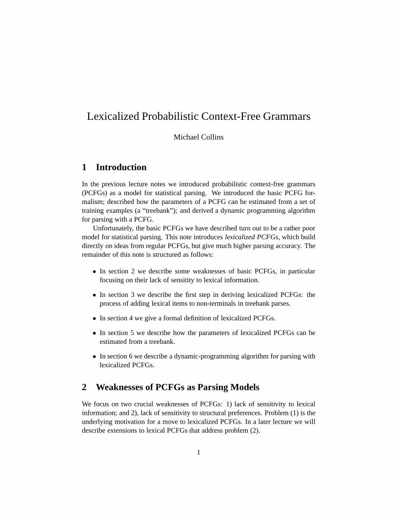
First, consider the following parse tree:S
NP
NNP
IBM
VP
VB
bought
NP
NNP
LotusUnder the PCFG model, this tree will have probability
q(S→ NP VP)× q(VP → V NP)× q(NP→ NNP)× q(NP→ NNP)
×q(NNP→ IBM)× q(Vt → bought)× q(NNP→ Lotus)
Recall that for any ruleα → β, q(α → β) is an associated parameter, which canbe interpreted as the conditional probability of seeingβ on the right-hand-side ofthe rule, given thatα is on the left-hand-side of the rule.
If we consider the lexical items in this parse tree (i.e.,IBM, bought, andLotus),we can see that the PCFG makes a very strong independence assumption. Intu-itively the identity of each lexical item depends only on thepart-of-speech (POS)above that lexical item: for example, the choice of the wordIBM depends on its tagNNP, but does not depend directly on other information in the tree. More formally,the choice of each word in the string is conditionally independent of the entire tree,once we have conditioned on the POS directly above the word. This is clearly avery strong assumption, and it leads to many problems in parsing. We will see thatlexicalized PCFGs address this weakness of PCFGs in a very direct way.
Let’s now look at how PCFGs behave under a particular type of ambiguity,prepositional-phrase (PP) attachment ambiguity. Figure 1shows two parse treesfor the same sentence that includes a PP attachment ambiguity. Figure 2 lists the setof context-free rules for the two parse trees. A critical observation is the following:the two parse trees have identical rules, with the exceptionof VP -> VP PPin tree (a), andNP -> NP PP in tree (b). It follows that the probabilistic parser,when choosing between the two parse trees, will pick tree (a)if
q(VP→ VP PP) > q(NP→ NP PP)
and will pick tree (b) if
q(NP→ NP PP) > q(VP→ VP PP)
2
(a) S
NP
NNS
workers
VP
VP
VBD
dumped
NP
NNS
sacks
PP
IN
into
NP
DT
a
NN
bin
(b) S
NP
NNS
workers
VP
VBD
dumped
NP
NP
NNS
sacks
PP
IN
into
NP
DT
a
NN
bin
Figure 1: Two valid parses for a sentence that includes a prepositional-phrase at-tachment ambiguity.
3
(a)
RulesS→ NP VPNP→ NNSVP → VP PPVP→ VBD NPNP→ NNSPP→ IN NPNP→ DT NNNNS→ workersVBD → dumpedNNS→ sacksIN → intoDT → aNN → bin
(b)
RulesS→ NP VPNP→ NNSNP → NP PPVP → VBD NPNP→ NNSPP→ IN NPNP→ DT NNNNS→ workersVBD → dumpedNNS→ sacksIN → intoDT → aNN → bin
Figure 2: The set of rules for parse trees (a) and (b) in figure 1.
Notice that this decision isentirely independent of any lexical information (thewords) in the two input sentences. For this particular case of ambiguity (NP vs VPattachment of a PP, with just one possible NP and one possibleVP attachment) theparser will always attach PPs to VP ifq(VP→ VP PP) > q(NP→ NP PP), andconversely will always attach PPs to NP ifq(NP→ NP PP) > q(VP→ VP PP).
The lack of sensitivity to lexical information in this particular situation, prepositional-phrase attachment ambiguity, is known to be highly non-optimal. The lexical itemsinvolved can give very strong evidence about whether to attach to the noun or theverb. If we look at the preposition,into, alone, we find that PPs withinto as thepreposition are almost nine times more likely to attach to a VP rather than an NP(this statistic is taken from the Penn treebank data). As another example, PPs withthe prepositionof are about 100 times more likely to attach to an NP rather than aVP. But PCFGs ignore the preposition entirely in making the attachment decision.
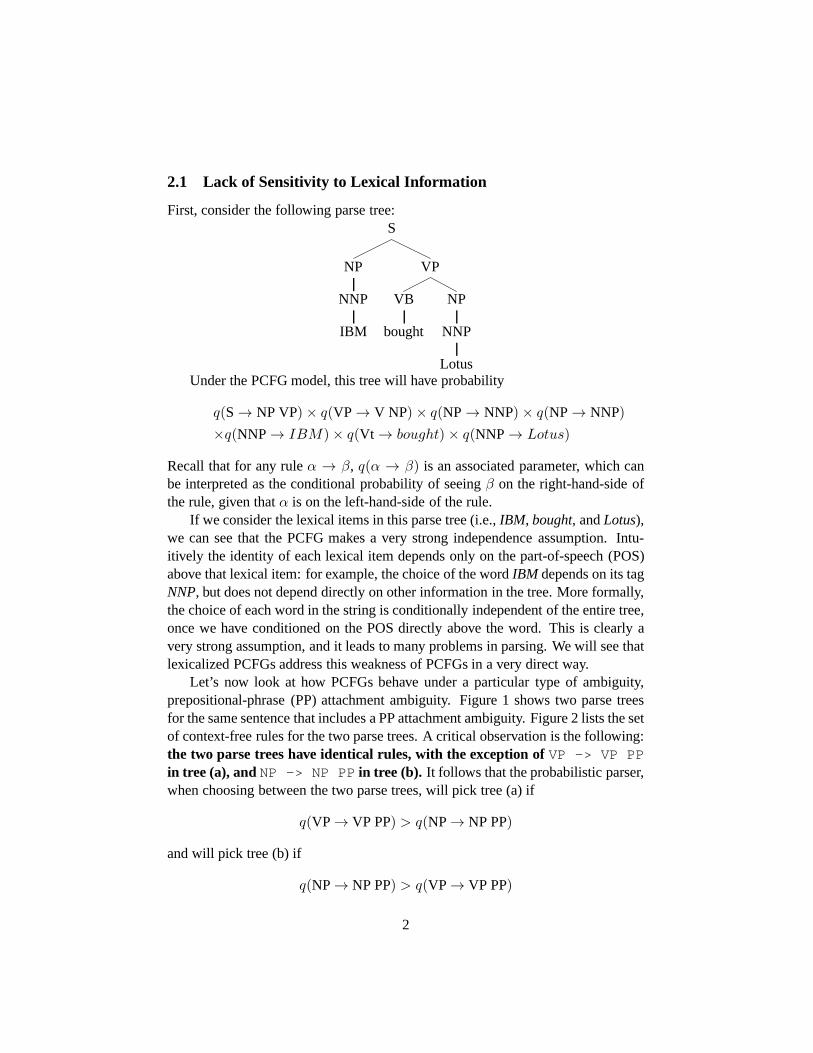
As another example, consider the two parse trees shown in figure 3, which is anexample of coordination ambiguity. In this case it can be verified that the two parsetrees have identical sets of context-free rules (the only difference is in the order inwhich these rules are applied). Hence a PCFG will assign identical probabilities tothese two parse trees, again completely ignoring lexical information.
In summary, the PCFGs we have described essentially generate lexical items asan afterthought, conditioned only on the POS directly abovethem in the tree. Thisis a very strong independence assumption, which leads to non-optimal decisionsbeing made by the parser in many important cases of ambiguity.
4
(a) NP
NP
NP
NNS
dogs
PP
IN
in
NP
NNS
houses
CC
and
NP
NNS
cats
(b) NP
NP
NNS
dogs
PP
IN
in
NP
NP
NNS
houses
CC
and
NP
NNS
cats
Figure 3: Two valid parses for a noun-phrase that includes aninstance of coordi-nation ambiguity.
5
(a) NP
NP
NN
president
PP
IN
of
NP
NP
DT
a
NN
company
PP
IN
in
NP
NN
Africa
(b) NP
NP
NP
NN
president
PP
IN
of
NP
DT
a
NN
company
PP
IN
in
NP
NN
Africa
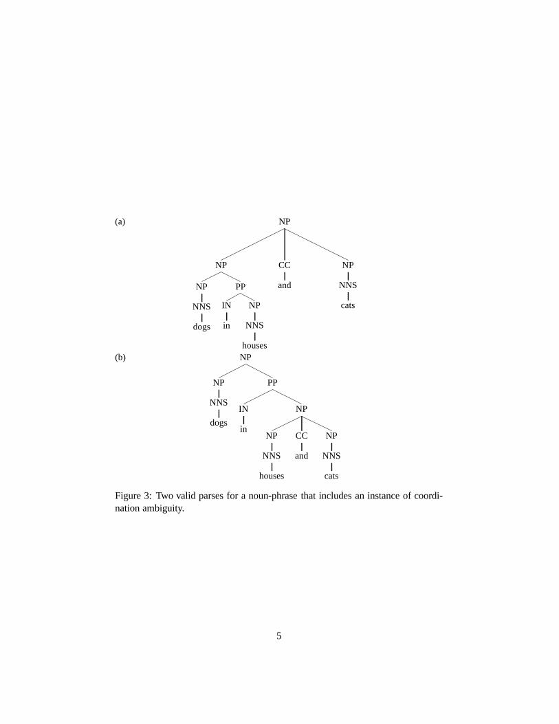
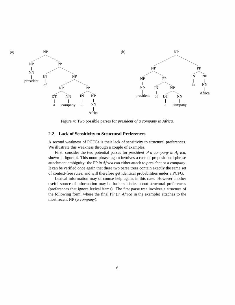
Figure 4: Two possible parses forpresident of a company in Africa.
2.2 Lack of Sensitivity to Structural Preferences
A second weakness of PCFGs is their lack of sensitivity to structural preferences.We illustrate this weakness through a couple of examples.
First, consider the two potential parses forpresident of a company in Africa,shown in figure 4. This noun-phrase again involves a case of prepositional-phraseattachment ambiguity: the PPin Africa can either attach topresidentor a company.It can be verified once again that these two parse trees contain exactly the same setof context-free rules, and will therefore get identical probabilities under a PCFG.
Lexical information may of course help again, in this case. However anotheruseful source of information may be basic statistics about structural preferences(preferences that ignore lexical items). The first parse tree involves a structure ofthe following form, where the final PP (in Africa in the example) attaches to themost recent NP (a company):
6
NP
NP
NN
PP
IN NP
NP
NN
PP
IN NP
NN
(1)
This attachment for the final PP is often referred to as aclose attachment, becausethe PP has attached to the closest possible preceding NP. Thesecond parse structurehas the form
NP
NP
NP
NN
PP
IN NP
NN
PP
IN NP
NN
(2)
where the final PP has attached to the further NP (presidentin the example).We can again look at statistics from the treebank for the frequency of structure 1
versus 2: structure 1 is roughly twice as frequent as structure 2. So there is a fairlysignificant bias towards close attachment. Again, we stressthat the PCFG assignsidentical probabilities to these two trees, because they include the same set of rules:hence the PCFG fails to capture the bias towards close-attachment in this case.
There are many other examples where close attachment is a useful cue in dis-ambiguating structures. The preferences can be even stronger when a choice isbeing made between attachment to two different verbs. For example, consider thesentence
John was believed to have been shot by Bill
Here the PPby Bill can modify either the verbshot(Bill was doing the shooting)or believe(Bill is doing the believing). However statistics from the treebank showthat when a PP can attach to two potential verbs, it is about 20times more likely
7
to attach to the most recent verb. Again, the basic PCFG will often give equalprobability to the two structures in question, because theycontain the same set ofrules.
3 Lexicalization of a Treebank
We now describe how lexicalized PCFGs address the first fundamental weakness ofPCFGs: their lack of sensitivity to lexical information. The first key step, describedin this section, is tolexicalizethe underlying treebank.
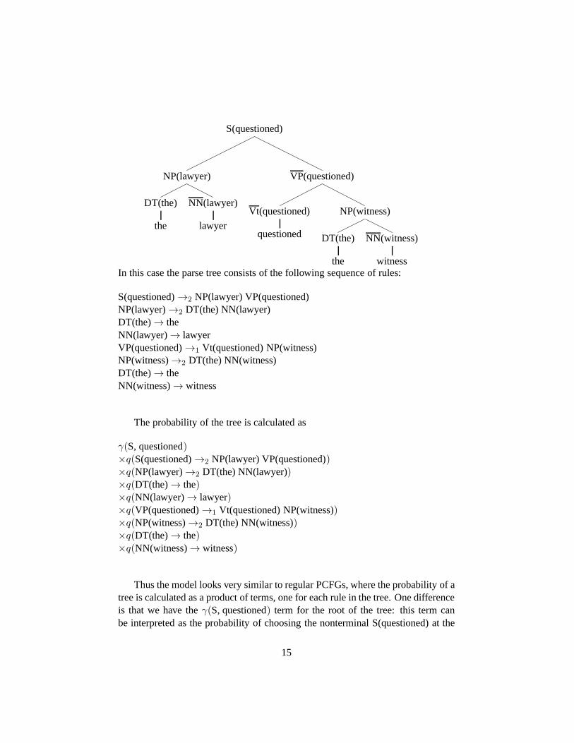
Figure 5 shows a parse tree before and after lexicalization.The lexicalizationstep has replaced non-terminals such asS or NP with new non-terminals that in-clude lexical items, for exampleS(questioned) or NP(lawyer).
The remainder of this section describes exactly how trees are lexicalized. Firstthough, we give the underlying motivation for this step. Thebasic idea will be toreplace rules such as
S→ NP VP
in the basic PCFG, with rules such as
S(questioned)→ NP(lawyer) VP(questioned)
in the lexicalized PCFG. The symbols S(questioned), NP(lawyer) and VP(questioned)are new non-terminals in the grammar. Each non-terminal nowincludes a lexicalitem; the resulting model has far more sensitivity to lexical information.
In one sense, nothing has changed from a formal standpoint: we will sim-ply move from a PCFG with a relatively small number of non-terminals (S, NP,etc.) to a PCFG with a much larger set of non-terminals (S(questioned),NP(lawyer) etc.) This will, however, lead to a radical increase in the num-ber of rules and non-terminals in the grammar: for this reason we will have to takesome care in estimating the parameters of the underlying PCFG. We describe howthis is done in the next section.
First, however, we describe how the lexicalization processis carried out. Thekey idea will be to identify for each context-free rule of theform
X → Y1 Y2 . . . Yn
an indexh ∈ {1 . . . n} that specifies theheadof the rule. The head of a context-free rule intuitively corresponds to the “center” or the most important child of therule.1 For example, for the rule
S→ NP VP1The idea of heads has a long history in linguistics, which is beyond the scope of this note.
8
(a) S
NP
DT
the
NN
lawyer
VP
Vt
questioned
NP
DT
the
NN
witness
(b)
S(questioned)
NP(lawyer)
DT(the)
the
NN(lawyer)
lawyer
VP(questioned)
Vt(questioned)
questioned
NP(witness)
DT(the)
the
NN(witness)
witness
Figure 5: (a) A conventional parse tree as found for example in the Penn treebank.(b) A lexicalized parse tree for the same sentence. Note thateach non-terminal inthe tree now includes a single lexical item. For clarity we mark the head of eachrule with an overline: for example for the ruleNP → DT NN the childNN is thehead, and hence theNN symbol is marked asNN.
9
the head would beh = 2 (corresponding to theVP). For the rule
NP→ NP PP PP PP
the head would beh = 1 (corresponding to theNP). For the rule
PP→ IN NP
the head would beh = 1 (corresponding to theIN), and so on.Once the head of each context-free rule has been identified, lexical information
can be propagated bottom-up through parse trees in the treebank. For example, ifwe consider the sub-tree
NP
DT
the
NN
lawyerand assuming that the head of the rule
NP→ DT NN
is h = 2 (theNN), the lexicalized sub-tree isNP(lawyer)
DT(the)
the
NN(lawyer)
lawyerParts of speech such asDT or NN receive the lexical item below them as their
head word. Non-terminals higher in the tree receive the lexical item from theirhead child: for example, theNP in this example receives the lexical itemlawyer,because this is the lexical item associated with theNN which is the head child oftheNP. For clarity, we mark the head of each rule in a lexicalized parse tree withan overline (in this case we haveNN). See figure 5 for an example of a completelexicalized tree.
As another example consider theVP in the parse tree in figure 5. Before lex-icalizing theVP, the parse structure is as follows (we have filled in lexical itemslower in the tree, using the steps described before):
10
VP
Vt(questioned)
questioned
NP(witness)
DT(the)
the
NN(witness)
witnessWe then identifyVt as the head of the rule VP→ Vt NP, and lexicalize the tree asfollows:
VP(questioned)
Vt(questioned)
questioned
NP(witness)
DT(the)
the
NN(witness)
witnessIn summary, once the head of each context-free rule has been identified, lexical
items can be propagated bottom-up through parse trees, to give lexicalized treessuch as the one shown in figure 5(b).
The remaining question is how to identify heads. Ideally, the head of eachrule would be annotated in the treebank in question: in practice however, theseannotations are often not present. Instead, researchers have generally used a simpleset of rules to automatically identify the head of each context-free rule.
As one example, figure 6 gives an example set of rules that identifies the headof rules whose left-hand-side isNP. Figure 7 shows a set of rules used forVPs.In both cases we see that the rules look for particular children (e.g.,NN for theNPcase,Vi for theVP case). The rules are fairly heuristic, but rely on some linguisticguidance on what the head of a rule should be: in spite of theirsimplicity theywork quite well in practice.
4 Lexicalized PCFGs
The basic idea in lexicalized PCFGs will be to replace rules such as
S→ NP VP
with lexicalized rules such as
S(examined)→ NP(lawyer) VP(examined)
11
If the rule contains NN, NNS, or NNP:Choose the rightmost NN, NNS, or NNP
Else If the rule contains an NP: Choose the leftmost NP
Else If the rule contains a JJ: Choose the rightmost JJ
Else If the rule contains a CD: Choose the rightmost CD
ElseChoose the rightmost child
Figure 6: Example of a set of rules that identifies the head of any rule whose left-hand-side is an NP.
If the rule contains Vi or Vt: Choose the leftmost Vi or Vt
Else If the rule contains a VP: Choose the leftmost VP
ElseChoose the leftmost child
Figure 7: Example of a set of rules that identifies the head of any rule whose left-hand-side is a VP.
12
Thus we have replaced simple non-terminals such asS or NP with lexicalized non-terminals such asS(examined) or NP(lawyer).
From a formal standpoint, nothing has changed: we can treat the new, lexi-calized grammar exactly as we would a regular PCFG. We have just expanded thenumber of non-terminals in the grammar from a fairly small number (say 20, or50) to a much larger number (because each non-terminal now has a lexical item,we could easily have thousands or tens of thousands of non-terminals).
Each rule in the lexicalized PCFG will have an associated parameter, for ex-ample the above rule would have the parameter
q(S(examined)→ NP(lawyer) VP(examined))
There are a very large number of parameters in the model, and we will have totake some care in estimating them: the next section describes parameter estimationmethods.
We will next give a formal definition of lexicalized PCFGs, inChomsky normalform. First, though, we need to take care of one detail. Each rule in the lexicalizedPCFG has a non-terminal with a head word on the left hand side of the rule: forexample the rule
S(examined)→ NP(lawyer) VP(examined)
hasS(examined) on the left hand side. In addition, the rule has two children.One of the two children must have the same lexical item as the left hand side:in this exampleVP(examined) is the child with this property. To be explicitabout which child shares the lexical item with the left hand side, we will add anannotation to the rule, using→1 to specify that the left child shares the lexical itemwith the parent, and→2 to specify that the right child shares the lexical item withthe parent. So the above rule would now be written as
S(examined)→2 NP(lawyer) VP(examined)
The extra notation might seem unneccessary in this case, because it is clearthat the second child is the head of the rule—it is the only child to have the samelexical item,examined, as the left hand side of the rule. However this informationwill be important for rules where both children have the samelexical item: take forexample the rules
PP(in)→1 PP(in) PP(in)
andPP(in)→2 PP(in) PP(in)
13
where we need to be careful about specifying which of the two children is the headof the rule.
We now give the following definition:
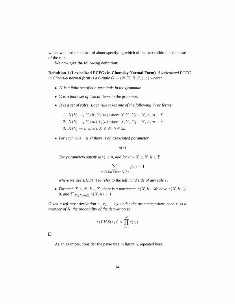
Definition 1 (Lexicalized PCFGs in Chomsky Normal Form) A lexicalized PCFGin Chomsky normal form is a 6-tupleG = (N,Σ, R, S, q, γ) where:
• N is a finite set of non-terminals in the grammar.
• Σ is a finite set of lexical items in the grammar.
• R is a set of rules. Each rule takes one of the following three forms:
Thus the model looks very similar to regular PCFGs, where theprobability of atree is calculated as a product of terms, one for each rule in the tree. One differenceis that we have theγ(S, questioned) term for the root of the tree: this term canbe interpreted as the probability of choosing the nonterminal S(questioned) at the
15
root of the tree. (Recall that in regular PCFGs we specified that a particular non-terminal, for exampleS, always appeared at the root of the tree.)
5 Parameter Estimation in Lexicalized PCFGs
We now describe a method for parameter estimation within lexicalized PCFGs.The number of rules (and therefore parameters) in the model is very large. How-ever with appropriate smoothing—using techniques described earlier in the class,for language modeling—we can derive estimates that are robust and effective inpractice.
First, for a given rule of the form
X(h) →1 Y1(h) Y2(m)
orX(h) →2 Y1(m) Y2(h)
define the following variables:X is the non-terminal on the left-hand side of therule;H is the head-word of that non-terminal;R is the rule used, either of the formX →1 Y1 Y2 orX →2 Y1 Y2; M is the modifier word.
For example, for the rule
S(examined)→2 NP(lawyer) VP(examined)
we have
X = S
H = examined
R = S→2 NP VP
M = lawyer
With these definitions, the parameter for the rule has the following interpreta-tion:
q(S(examined)→2 NP(lawyer) VP(examined))
= P (R = S→2 NP VP,M = lawyer|X = S,H = examined)
The first step in deriving an estimate ofq(S(examined)→2 NP(lawyer) VP(examined))will be to use the chain rule to decompose the above expression into two terms:
whereλ1 dictates the relative weights of the two estimates (we have0 ≤ λ1 ≤ 1).The value forλ1 can be estimated using the methods described in the notes onlanguage modeling for this class.
Next, consider our estimate of the expression in Eq. 4. We candefine thefollowing two maximum-likelihood estimates:
where0 ≤ λ2 ≤ 1 is a parameter specifying the relative weights of the two terms.Putting these estimates together, our final estimate of the rule parameter is as
It can be seen that this estimate combines very lexically-specific information, forexample the estimates
qML(S→2 NP VP|S, examined)
qML(lawyer|S→2 NP VP, examined)
with estimates that rely less on lexical information, for example
qML(S→2 NP VP|S)
qML(lawyer|S→2 NP VP)
The end result is a model that is sensitive to lexical information, but which is never-theless robust, because we have used smoothed estimates of the very large numberof parameters in the model.
6 Parsing with Lexicalized PCFGs
The parsing algorithm for lexicalized PCFGs is very similarto the parsing algo-rithm for regular PCFGs, as described in the previous lecture notes. Recall thatfor a regular PCFG the dynamic programming algorithm for parsing makes use ofa dynamic programming tableπ(i, j,X). Each entryπ(i, j,X) stores the high-est probability for any parse tree rooted in non-terminalX, spanning wordsi . . . jinclusive in the input sentence. Theπ values can be completed using a recursivedefinition, as follows. Assume that the input sentence to thealgorithm isx1 . . . xn.The base case of the recursion is fori = 1 . . . n, for all X ∈ N ,
π(i, i,X) = q(X → xi)
where we defineq(X → xi) = 0 if the ruleX → xi is not in the grammar.The recursive definition is as follows: for any non-terminalX, for anyi, j such
that1 ≤ i < j ≤ n,
π(i, j,X) = maxX→Y Z,s∈{i...(j−1)}
q(X → Y Z)× π(i, s, Y )× π(s+ 1, j, Z)
Thus we have amax over all rulesX → Y Z, and all split-pointss ∈ {i . . . (j −1)}. This recursion is justified because any parse tree rooted inX, spanning wordsi . . . j, must be composed of the following choices:
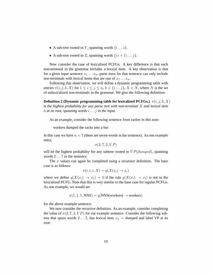
Now consider the case of lexicalized PCFGs. A key differenceis that eachnon-terminal in the grammar includes a lexical item. A key observation is thatfor a given input sentencex1 . . . xn, parse trees for that sentence can only includenon-terminals with lexical items that are one ofx1 . . . xn.
Following this observation, we will define a dynamic programming table withentriesπ(i, j, h,X) for 1 ≤ i ≤ j ≤ n, h ∈ {i . . . j}, X ∈ N , whereN is the setof unlexicalized non-terminals in the grammar. We give the following definition:
Definition 2 (Dynamic programming table for lexicalized PCFGs.) π(i, j, h,X)is the highest probability for any parse tree with non-terminal X and lexical itemh at its root, spanning wordsi . . . j in the input.
As an example, consider the following sentence from earlierin this note:
workers dumped the sacks into a bin
In this case we haven = 7 (there are seven words in the sentence). As one exampleentry,
π(2, 7, 2, V P )
will be the highest probability for any subtree rooted inV P (dumped), spanningwords2 . . . 7 in the sentence.
The π values can again be completed using a recursive definition. The basecase is as follows:
π(i, i, i,X) = q(X(xi) → xi)
where we defineq(X(xi) → xi) = 0 if the rule q(X(xi) → xi) is not in thelexicalized PCFG. Note that this is very similar to the base case for regular PCFGs.As one example, we would set
π(1, 1, 1,NNS) = q(NNS(workers)→ workers)
for the above example sentence.We now consider the recursive definition. As an example, consider completing
the value ofπ(2, 7, 2, V P ) for our example sentence. Consider the following sub-tree that spans words2 . . . 7, has lexical itemx2 = dumped and label VP at itsroot:
19
VP(dumped)
VP(dumped)
VBD(dumped)
dumped
NP(sacks)
DT(the)
the
NNS(sacks)
sacks
PP(into)
IN(into)
into
NP(bin)
DT(a)
a
NN(bin)
bin
We can see that this subtree has the following sub-parts:
• A choice of split-points ∈ {1 . . . 6}. In this case we chooses = 4 (the splitbetween the two subtrees under the rule VP(dumped)→1 VBD(dumped) PP(into)is afterx4 = sacks).
• A choice of modifier wordm. In this case we choosem = 5, correspondingto x5 = into, becausex5 is the head word of the second child of the ruleVP(dumped)→1 VBD(dumped) PP(into).
• A choice of rule at the root of the tree: in this case the rule isVP(dumped)→1 VBD(dumped) PP(into).
More generally, to find the value for anyπ(i, j, h,X), we need to search overall possible choices fors, m, and all rules of the formX(xh) →1 Y1(xh) Y2(xm)or X(xh) →2 Y1(xm) Y2(xh). Figure 8 shows pseudo-code for this step. Notethat some care is needed when enumerating the possible values fors andm. If s isin the rangeh . . . (j − 1) then the head wordh must come from the left sub-tree; itfollows thatm must come from the right sub-tree, and hence must be in the range(s + 1) . . . j. Conversely, ifs is in the rangei . . . (h − 1) thenm must be in theleft sub-tree, i.e., in the rangei . . . s. The pseudo-code in figure 8 treats these twocases separately.
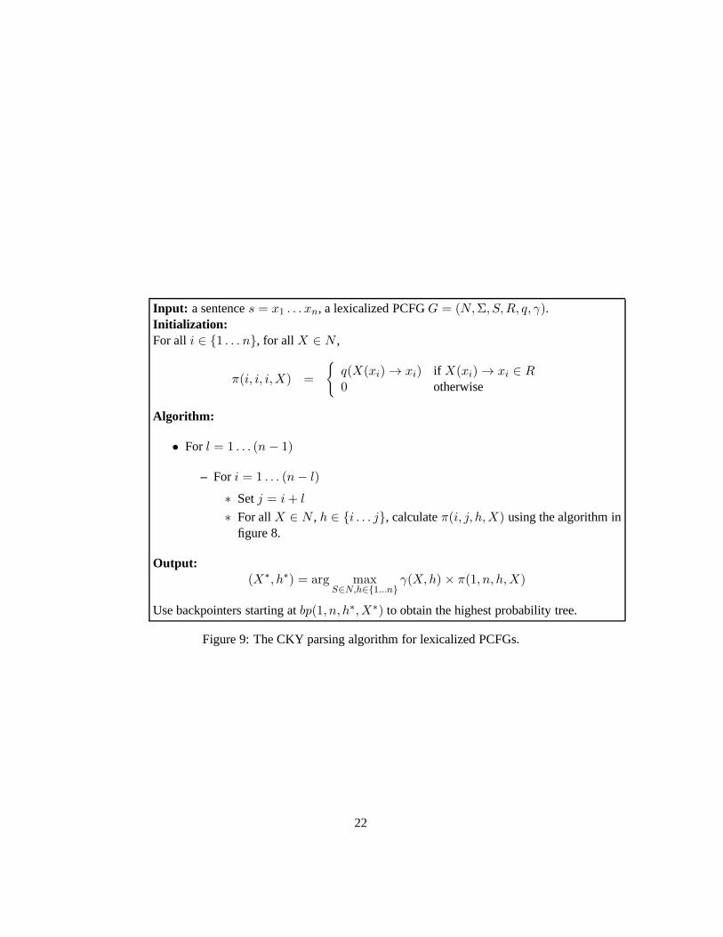
Figure 9 gives the full algorithm for parsing with lexicalized PCFGs. Thealgorithm first completes the base case of the recursive definition for theπ values.It then fills in the rest of theπ values, starting with the case wherej = i+ 1, thenthe casej = i+ 2, and so on. Finally, the step
(X∗, h∗) = arg maxX∈N,h∈{1...n}
γ(X,h) × π(1, n, h,X)
finds the pairX∗(h∗) which is at the root of the most probable tree for the input sen-tence: note that theγ term is taken into account at this step. The highest probabilitytree can then be recovered by following backpointers starting atbp(1, n, h∗,X∗).
20
1. π(i, j, h,X) = 0
2. Fors = h . . . (j − 1), for m = (s+1) . . . j, for X(xh) →1 Y (xh)Z(xm) ∈R,
(a) p = q(X(xh) →1 Y (xh)Z(xm))× π(i, s, h, Y )× π(s+ 1, j,m,Z)
(b) If p > π(i, j, h,X),π(i, j, h,X) = p
bp(i, j, h,X) = 〈s,m, Y, Z〉
3. Fors = i . . . (h− 1), for m = i . . . s, for X(xh) →2 Y (xm)Z(xh) ∈ R,
(a) p = q(X(xh) →2 Y (xm)Z(xh))× π(i, s,m, Y )× π(s+ 1, j, h, Z)
(b) If p > π(i, j, h,X),π(i, j, h,X) = p
bp(i, j, h,X) = 〈s,m, Y, Z〉
Figure 8: The method for calculating an entryπ(i, j, h,X) in the dynamic pro-gramming table. The pseudo-code searches over all split-points s, over all mod-ifier positionsm, and over all rules of the formX(xh) →1 Y (xh) Z(xm) orX(xh) →2 Y (xm) Z(xh). The algorithm stores backpointer valuesbp(i, j, h,X).
21
Input: a sentences = x1 . . . xn, a lexicalized PCFGG = (N,Σ, S,R, q, γ).Initialization:For all i ∈ {1 . . . n}, for all X ∈ N ,
π(i, i, i,X) =
{
q(X(xi) → xi) if X(xi) → xi ∈ R
0 otherwise
Algorithm:
• For l = 1 . . . (n − 1)
– For i = 1 . . . (n− l)
∗ Setj = i+ l
∗ For allX ∈ N , h ∈ {i . . . j}, calculateπ(i, j, h,X) using the algorithm infigure 8.
Output:(X∗, h∗) = arg max
S∈N,h∈{1...n}γ(X,h) × π(1, n, h,X)
Use backpointers starting atbp(1, n, h∗,X∗) to obtain the highest probability tree.
Figure 9: The CKY parsing algorithm for lexicalized PCFGs.