290


Butterworth-Heinemann is an imprint of ElsevierLinacre House, Jordan Hill, Oxford OX2 8DP, UK30 Corporate Drive, Suite 400, Burlington, MA 01803, USA
First edition 2009
Copyright © 2009, Elsevier Ltd. All rights reserved
No part of this publication may be reproduced, stored in retrieval system or transmit-ted in any form or by any means electronic, mechanical, photocopying, recording or otherwise without the prior written permission of the publisher
Permissions may be sought directly from Elsevier’s Science & Technology Rights Department in Oxford, UK: phone: (44) (0) 1865 843830, fax: (44) (0) 1865 853333, e-mail: [email protected]. Alternatively you can submit your request online by visiting the Elsevier web site at http://elsevier.com/locate/permission, and selecting Obtaining permission to use Elsevier material
NoticeNo responsibility is assumed by the publisher for any injury and/or damage to persons or property as a matter of products liability, negligence or otherwise, or from any use or operation of any methods, products, instructions or ideas contained in the material herein. Because of rapid advances in the medical sciences, in particular, independent verification of diagnoses and drug dosages should be made
British Library Cataloguing in Publication DataA catalogue record for this book is available from the British Library
Library of Congress Cataloging in Publication DataA catalogue record for this book is available from the Library of Congress
ISBN–13: 978-1-85617-517-3
For information on all Butterworth-Heinemann Publicationsvisit our web site at www.elsevierdirect.com
Printed and bound in Great Britain09 10 11 12 13 10 9 8 7 6 5 4 3 2 1
Preface
Atomic force microscopy (AFM) was first described in the scientific lit-erature in 1986. It arose as a development of scanning tunnelling micros-copy (STM). However, whereas STM is only capable of imaging conductive samples in vacuum, AFM has the capability of imaging surfaces at high resolution in both air and liquids. As these correspond to the conditions under which virtually all surfaces exist in the real world, this greatly increased the potentially useful role of scanning probe microscopies. This great potential of AFM led to its very rapid development. By the early 1990s, it was moving outside of specialist physics laboratories and the first commercial instruments were becoming available.
At the time, our main process engineering research activities were in the fields of membrane separation processes and colloid processing. Both of these fields involve the manipulation of materials on the micrometre to the nanometre length scales. To image the materials used in such processes, we used scanning electron microscopy, which was expensive, time-consuming, and even more undesirably usually involved complex sample preparation procedures and measurement in vacuum which could result in undesirable experimental artefacts. Our imagination was fired and our research greatly facilitated, following an inspiring lecture given by Jacob Israelachvili at the 7th International Conference on Surface and Colloid Science in Compiègne, France, in July 1991, in which he described some of the very first appli-cations of AFM in colloid science. Our first grant application for AFM equipment was written very shortly afterwards!
Since that time there has been an enormous development of the capa-bilities and applicability of AFM. Physicists have devised a bewilder-ing range of experimental techniques for probing the different properties of surfaces. Scientists, especially those working in the biological sciences, have been able to make remarkable discoveries using AFM that would have been otherwise unobtainable. A huge amount of scientific literature has appeared including a number of introductory and advanced books. However, despite the achievements and great potential for the application of AFM to process engineering, there is no book-length text describing such achievements and applications. Further, the specialist nature of the primary literature and the disciplinary strangeness of the existing book-length texts can appear rather formidable to engineers who might wish to apply AFM
ix

x Preface
in their work. Hence, it is our assessment that the benefit of AFM to the development of process engineering is under-fulfilled. Nevertheless, the significant decrease in cost of commercial AFM equipment, and its increas-ing ‘user-friendliness’, has made the technique readily accessible to most engineers. We were, therefore, motivated to put together the present text with the specific intention of describing the achievements and possibilities of AFM in a way which is directly relevant to the work of our process engineering colleagues, with the hope that we will inspire them to apply this remarkable technique for the benefit of their own activities.
We begin in Chapter 1 by providing an outline of the basic principles of AFM. The chapter introduces the main features of AFM equipment and describes the imaging modes which are most likely to be of benefit in process engineering applications. Such knowledge of the main operating modes should allow the reader to interpret the nature of the many subtle variations described in the primary research literature. We also introduce a remarkable benefit of AFM equipment, because it is a force microscope it can be used to directly measure surface interactions with very high reso-lution in both force and distance. An especially useful application of this capability is the use of ‘colloid probes’, the nature of which is introduced and the benefits of which become apparent in several of the later chapters.
AFM can generate beautiful images of surfaces at subnanometre resolu-tion. However, the detailed interpretation of the features of such images can benefit greatly from an understanding of the fundamental interactions from which they arise. This is the subject of Chapter 2. Depending on the materials being investigated and the experimental conditions, the interac-tions which give rise to such images, either separately or simultaneously, include van der Waals forces, electrical double layer forces, hydrophobic interactions, solvation forces, steric interactions, hydrodynamic drag forces and adhesion. AFM also has the capability to quantify such interactions, especially using colloid probe techniques. For this reason, mathematical descriptions of such interactions are given in forms which have proved of practical use in process engineering.
Once the basics of AFM have been outlined, it is possible to move to a description of specific applications. Process engineering is a diverse and growing field comprising both established processes of great soci-etal significance and new areas of huge promise. We begin in Chapter 3 by describing investigations of an established and important type of phenomenon – the quantification of particle–bubble interactions. Such interactions are of fundamental significance in some of the largest-scale industrial processes, most notably in mineral processing and in wastewater treatment. It is especially the capability of AFM equipment to quantify the interactions between bubbles and micrometre size particles that can lead to the development of processes of increased flotation efficiency and greater specificity of separation. This is a remarkable example of how nanoscale interactions control the efficiency of megascale processes.
Preface xi
Membrane separation processes are one of the most significant develop-ments in process engineering in recent times. They now find widespread application in fields as diverse as water treatment, pharmaceutical pro-cessing, food processing, biotechnology, sensors and batteries. Membranes are most usually thin polymeric sheets, having pores in the range from the micrometre to subnanometre, that act as advanced filtration materials. Their separation capabilities are due to steric effects and the whole range of interactions that can be probed by AFM. Hence, there is a very close match between the factors that control the effectiveness of a membrane process and the measurement capabilities of AFM. In Chapter 4, we pro-vide a survey of the numerous ways in which AFM can be used to study the factors controlling membrane processes. We consider both advanced imaging and force measurement techniques, and how they may be com-bined, for example, to provide a ‘visualisation’ of the rejection of a colloid particle by a membrane pore. Chapter 5 is more especially concerned with the use of AFM in the development of new membranes with specifically desirable properties. We focus, in particular, on the development of foul-ing resistant membranes, i.e. membranes with the minimum of unwanted adhesion of substances from the fluids being processed.
In the pharmaceutical industry, there is an increasing drive to develop new ways of drug delivery, both means for the presentation of drugs to the patient and of drug formulations which target specific sites in the body. Both of these goals can benefit from knowledge of structures and interactions at the nanoscale. Thus, pharmaceutical development can benefit from both the imaging and force measurement capabilities of AFM, as described in Chapter 6. The colloid probe, or more precisely drug particle probe, techniques are again very important in this work. However, there is also scope for the use of advanced techniques, such as micro- and nanothermal characterisation using a scanning thermal microscope (SThM), which can provide spatial information at a resolu-tion unavailable to conventional calorimetry.
Bioprocessing is acquiring a sophistication that was unimaginable even a few years ago. An important example is given in Chapter 7. Cells sense and respond to their surrounding microenvironment. The chapter reviews the application of micro/nanoengineering and AFM to the investigation of cell response in engineered microenvironments that mimic the natural extracellular matrix. In particular, the chapter reports the use of micro/nanoengineering to make structures that aid the understanding of funda-mental cellular interactions, which in turn help further development of new therapeutic methods. Specific attention is given to the combination of AFM with optical microscopy for the simultaneous interrogation of biophysical and biochemical cellular processes and properties, as well as the quantification of cell viscoelasticity.
Throughout the process industries, and more generally in manufac-turing, the surfaces of materials are modified with coatings to protect
xii Preface
them from hostile conditions and to functionalise them for a variety of purposes. In particular, ultrathin coatings play a crucial role in many processes, ranging from protection against chemical corrosion to micro-fabrication for microelectronics and biomedical devices. Chapter 8 describes the use of AFM for the study of the fine structure and local nanomechanical properties of such advanced polymer monolayers and submonolayers. AFM allows the real-time/real-space monitoring of rel-evant physicochemical surface processes. As miniaturisation of electronic and medical devices approaches the nanometre scale, AFM is becom-ing the most important characterisation tool of their nanostructural and nanomechanical properties.
AFM has been considered primarily as a technique for the investiga-tion of the surfaces of solid materials, with the considerable benefit that it can be used to carry out such investigations in liquid environments. However, AFM may also be used to study the properties of such liquids themselves. This is the topic of Chapter 9, which describes dynamic stud-ies of confined fluids, micro- and nanorheology, cavitation and adhesive failure in thin films, and meso-scale experimental studies of the tensile behaviour of thin fluid films. Such studies benefit considerably from the coupling of AFM with high-magnification optical microscopy and high-speed video techniques. The development of such studies may be of con-siderable importance for the many large-scale processes that depend on the properties of thin liquid films, and also for instances where the avail-able quantities of fluids are tiny, such as for synovial fluid.
In the final chapter, we have pooled the thoughts of the contributors to provide a vision of some of the ways in which AFM may contribute to the development of process engineering in the future.
We thank all of the authors who have collaborated in the writing of this volume. We are very grateful for their willingness to devote time to this task and for their timely delivery of high-quality manuscripts. We also thank the many colleagues and research students who have con-tributed to the work described. Particular thanks are due to Dr Peter M. Williams. Peter worked as a research technician at our centre when we first started AFM studies. The results of our research as presented in this volume owe much to his technical ingenuity and patience.
W. Richard Bowen and Nidal [email protected]
[email protected] and England
February 2009

About the Editors
Professor W. Richard Bowen is a Fellow of the UK Royal Academy of Engineering. His work in chemical and biochemical engineering is widely recognised as world leading, particularly in the application of atomic force microscopy and in the development of membrane processes. He holds chairs in the Schools of Engineering at the University of Wales Swansea and the University of Surrey. He has carried out extensive consultancy for industry, government departments, research councils and universities on an international basis, currently through i-NewtonWales.
xiii

xiv About thE Editors
Professor Nidal Hilal is a Fellow of the Institution of Chemical Engineers and currently the Director of the Centre for Clean Water Technologies at the University of Nottingham. He obtained a PhD in Chemical Engineering from the University of Wales in 1988. Over the years, he has made a major contribution becoming an internationally leading expert in the application of Atomic Force Microscopy in process engineering and membrane technology. Professor Hilal is the author of over 300 refereed publications, including 4 textbooks and 11 invited chapters in interna-tional handbooks. In recognition of his substantial and sustained contri-bution to scientific knowledge, he was awarded a senior doctorate, Doctor of Science (DSc), from the University of Wales and the Kuwait Prize for Water Resources Development in 2005. He is a member of the editorial boards for a number of international journals and an advisor for interna-tional organizations including the Lifeboat Foundation. He is also on the panel of referees for the UK and international Research Councils.
Professor Hilal acknowledges His Majesty King Abdullah Bin Abdul Aziz Al-Saud of Saudi Arabia, who is a keen advocate for nanotechnol-ogy and process engineering, particularly in the field of desalination and water research for the benefit of all humanity.

List of Contributors
Prof. W. Richard Bowen, FREngi-NewtonWales, 54 Llwyn y mor, Caswell, Swansea, SA3 4RD, [email protected]
Prof. Nidal Hilal, DScDirector of Centre for Clean Water Technologies, Faculty of Engineering, University of Nottingham, University Park, Nottingham NG7 2RD, [email protected]
Prof. Clive J. RobertsDirector of Nottingham Nanotechnology and Nanoscience Centre, University of Nottingham, Nottingham NG7 2RD, [email protected]
Dr Huabing YinDepartment of Electronic and Electrical Engineering, University of Glasgow, Glasgow, [email protected]
Dr Vasileios KoutsosInstitute for Materials and Processes, School of Engineering and Centre for Materials Science & Engineering, The University of Edinburgh, The King’s Buildings, Edinburgh EH9 3JL, [email protected]
Prof. P. Rhodri WilliamsMultidisciplinary Nanotechnology Centre, School of Engineering, Swansea University, Singleton Park, Swansea SA2 8PP, [email protected]
Dr Paul Melvyn WilliamsMultidisciplinary Nanotechnology Centre, School of Engineering, Swansea University, Singleton Park, Swansea SA2 8PP, [email protected]
Dr Matthew BarrowMultidisciplinary Nanotechnology Centre, School of Engineering, Swansea University, Singleton Park, Swansea SA2 8PP, [email protected]
xv

xvi List of Contributors
Dr Daniel JohnsonCentre for Clean Water Technologies, Faculty of Engineering, The University of Nottingham, University Park, Nottingham, NG7 2RD, [email protected]
Gordon McPheeDepartment of Electronic and Electrical Engineering, University of Glasgow, [email protected]
Dr Phil DobsonDepartment of Electronic and Electrical Engineering, University of Glasgow, [email protected]

Atomic Force Microscopy in Process Engineering ©2009,ElsevierLtd�
O U T L I N E
�.� Introduction 2
�.2 The atomic force microscope 3
�.3 Cantilevers and probes 61.3.1 Effect of Probe Geometry 7
�.4 Imaging modes 81.4.1 Contact Mode Imaging 91.4.2 Intermittent Contact (Tapping) Mode 101.4.3 Non-Contact Mode 101.4.4 Force Volume Imaging 111.4.5 Force Modulation Mode 121.4.6 Lateral/Frictional Force Mode 12
�.5 The afm as a force sensor �2
�.6 Calibration of afm microcantilevers �61.6.1 Calibration of Normal spring Constants 161.6.2 Calibration of Torsional and Lateral spring Constants 21
�.7 Colloid probes 22
abbreviations and symbols 23References 24
BasicPrinciplesofAtomicForceMicroscopy
Daniel Johnson, Nidal Hilal and W. Richard Bowen
�C H A P T E R
2 1. BAsICPRINCIPLEsOFATOMICFORCEMICROsCOPy
�.� InTroduCTIon
The atomic force microscope (AFM), also referred to as the scanning force microscope (SFM), is part of a larger family of instruments termed the scanning probe microscopes (SPMs). These also include the scanning tunnelling microscope (STM) and scanning near field optical microscope (SNOM), amongst others. The common factor in all SPM techniques is the use of a very sharp probe, which is scanned across a surface of inter-est, with the interactions between the probe and the surface being used to produce a very high resolution image of the sample, potentially to the sub-nanometre scale, depending upon the technique and sharpness of the probe tip. In the case of the AFM the probe is a stylus which inter-acts directly with the surface, probing the repulsive and attractive forces which exist between the probe and the sample surface to produce a high-resolution three-dimensional topographic image of the surface.
The AFM was first described by [1]Binnig et al. as a new technique for imaging the topography of surfaces to a high resolution. It was cre-ated as a solution to the limitations of the STM, which was able to image only conductive samples in vacuum. Since then the AFM has enjoyed an increasingly ubiquitous role in the study of surface science, as both an imaging and surface characterisation technique, and also as a means of probing interaction forces between surfaces or molecules of interest by the application of force to these systems. The AFM has a number of advantages over electron microscope techniques, primarily its versatility in being able to take measurements in air or fluid environments rather than in high vacuum, which allows the imaging of polymeric and bio-logical samples in their native state. In addition, it is highly adaptable with probes being able to be chemically functionalised to allow quan-titative measurement of interactions between many different types of materials – a technique often referred to as chemical force microscopy.
At the core of an AFM instrument is a sharp probe mounted near to the end of a flexible microcantilever arm. By raster-scanning this probe across a surface of interest and simultaneously monitoring the deflection of this arm as it meets the topographic features present on the surface, a three-dimensional picture can be built up of the surface of the sample to a high resolution. Many different variations of this basic technique are currently used to image surfaces using the AFM, depending upon the properties of the sample and the information to be extracted from it. These variations include ‘static’ techniques such as contact mode, where the probe remains in constant contact with the sample, and ‘dynamic’ modes, where the cantilever may be oscillated, such as with the intermit-tent or non-contact modes. The forces of interaction between the probe and the sample may also be measured as a function of distance by the

1.2 THEATOMICFORCEMICROsCOPE 3
monitoring of the deflection of the cantilever, providing that the spring constant of the lever arm is sufficiently calibrated.
In this chapter the basic principles of operation of an AFM will be pre-sented, outlining the most common imaging modes and describing the acquisition of force distance measurements and techniques to calibrate cantilever spring constants.
�.2 The aTomIC forCe mICrosCope
In Figure 1.1 the basic set-up of a typical AFM is shown. Cantilevers are commonly either V-shaped, as shown, or a rectangular, ‘diving board’ shaped. The cantilever has at its free end a sharp tip, which acts as the probe of interactions. This probe is most commonly in the form of a square-based pyramid or a cylindrical cone. A few examples of dif-ferent configurations for levers and probes are shown in Figure 1.2. Commercially manufactured probes and cantilevers are predominantly of silicon nitride (the formula normally given for silicon nitride is Si3N4, although the precise stoichiometry may vary depending on the manufac-turing process) or silicon (Si). Typically the upper surface of the cantile-ver, opposite to the tip, is coated with a thin reflective surface, usually of either gold (Au) or aluminium (Al).
The probe is brought into and out of contact with the sample surface by the use of a piezocrystal upon which either the cantilever chip or the surface itself is mounted, depending upon the particular system being
fIgure �.� Basic AFM set-up. A probe is mounted at the apex of a flexible Si or Si3N4 cantilever. The cantilever itself or the sample surface is mounted on a piezocrystal which allows the position of the probe to be moved in relation to the surface. Deflection of the cantilever is monitored by the change in the path of a beam of laser light deflected from the upper side of the end of the cantilever by a photodetector. As the tip is brought into contact with the sample surface, by the movement of the piezocrystal, its deflection is monitored. This deflection can then be used to calculate interaction forces between probe and sample.
Sample surfaceChip
z
x
y
Cantilever
Light source
Probe
Light path
Photodetector
A B
C D

4 1. BAsICPRINCIPLEsOFATOMICFORCEMICROsCOPy
used (these two configurations are referred to as tip-scanning or surface-scanning, respectively). Movement in this direction is conventionally referred to as the z-axis. A beam of laser light is reflected from the reverse (uppermost) side of the cantilever onto a position-sensitive photodetector. Any deflection of the cantilever will produce a change in the position of the laser spot on the photodetector, allowing changes to the deflection to be monitored. The most common configuration for the photodetector is that of a quadrant photodiode divided into four parts with a horizontal and a vertical dividing line. If each section of the detector is labelled A to D as shown in Figure 1.1, then the deflection signal is calculated by the difference in signal detected by the A B versus C D quadrants. Comparison of the signal strength detected by A C versus B D will allow detection of lateral or torsional bending of the lever. Once the probe is in contact with the surface, it can then be raster-scanned across the surface to build up relative height information of topographic features of the sample.
fIgure �.2 Example of SEM images of different probes and cantilever types. A: pyramidal probe; B: conical high aspect ratio probe for high resolution imaging; C: two V-shaped cantilevers for contact mode imaging; D: chip with a series of beam-shaped levers of different lengths. In this case the levers are tipless to allow mounting of particles of inter-est for force measurements.
C D
A B

1.2 THEATOMICFORCEMICROsCOPE 5
This ‘optical lever’ method to detect deflection of the cantilever is the method primarily in use currently [2, 3]. However, the original design for the AFM used an STM piggy-backed onto the upper side of the AFM as a deflection sensor [1]. Whilst this allowed extremely accurate deter-mination of the deflection, it also could detect deflection only within a very small range, which is insufficient for most purposes. In addition, other methods have been trialled in the past for this purpose including the measurement of optical interferometry effects [4] as well as fabricat-ing levers to be able to detect deflection through a piezoresistance-based mechanism [5–14].
Scanners are available in different configurations, depending upon the particular AFM employed, or the purpose for which it is required. Tube scanners consist of a hollow tube made of piezoceramic material. Depending on how electrical current is applied, the tube may extend in the z-direction or be caused to flex in either the x- or y-direction to facili-tate scanning. Alternatively scanners may consist of separate piezocrys-tals for each movement direction. Such a configuration removes certain non-linearity problems, which may occur in the simpler tube scanners. In many commercially available AFMs, especially in older models, the movement in the x- and y-directions may be achieved by the movement of the sample rather than by the movement of the probe.
fIgure �.3 Diagram illustrating the force regimes under which each of the three most common AFM imaging modes operate. Contact mode operation is in the repulsive force regime, where the probe is pressed against the sample surface, causing an upwards deflec-tion of the cantilever. Non-contact mode interrogates the long-range forces experienced prior to actual contact with the surface. With intermittent contact, or tapping mode, the probe is oscillated close to the surface where it repeatedly comes into and out of contact with the surface.
Forc
e
Distance
Contact mode
Attraction
Repulsion
Non-contact mode
Intermittentcontact mode
6 1. BAsICPRINCIPLEsOFATOMICFORCEMICROsCOPy
�.3 CanTIlevers and probes
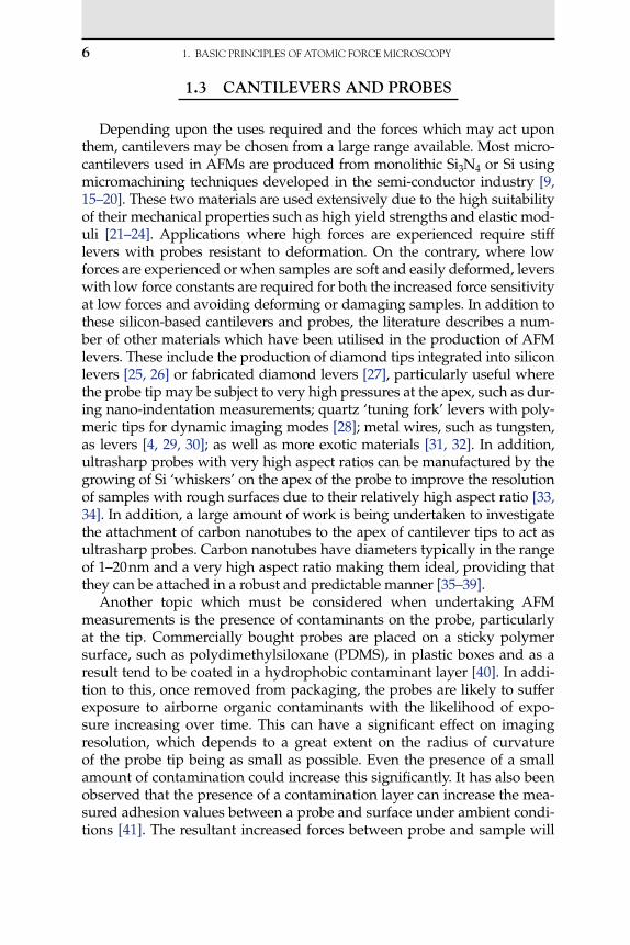
Depending upon the uses required and the forces which may act upon them, cantilevers may be chosen from a large range available. Most micro-cantilevers used in AFMs are produced from monolithic Si3N4 or Si using micromachining techniques developed in the semi-conductor industry [9, 15–20]. These two materials are used extensively due to the high suitability of their mechanical properties such as high yield strengths and elastic mod-uli [21–24]. Applications where high forces are experienced require stiff levers with probes resistant to deformation. On the contrary, where low forces are experienced or when samples are soft and easily deformed, levers with low force constants are required for both the increased force sensitivity at low forces and avoiding deforming or damaging samples. In addition to these silicon-based cantilevers and probes, the literature describes a num-ber of other materials which have been utilised in the production of AFM levers. These include the production of diamond tips integrated into silicon levers [25, 26] or fabricated diamond levers [27], particularly useful where the probe tip may be subject to very high pressures at the apex, such as dur-ing nano-indentation measurements; quartz ‘tuning fork’ levers with poly-meric tips for dynamic imaging modes [28]; metal wires, such as tungsten, as levers [4, 29, 30]; as well as more exotic materials [31, 32]. In addition, ultrasharp probes with very high aspect ratios can be manufactured by the growing of Si ‘whiskers’ on the apex of the probe to improve the resolution of samples with rough surfaces due to their relatively high aspect ratio [33, 34]. In addition, a large amount of work is being undertaken to investigate the attachment of carbon nanotubes to the apex of cantilever tips to act as ultrasharp probes. Carbon nanotubes have diameters typically in the range of 1–20 nm and a very high aspect ratio making them ideal, providing that they can be attached in a robust and predictable manner [35–39].
Another topic which must be considered when undertaking AFM measurements is the presence of contaminants on the probe, particularly at the tip. Commercially bought probes are placed on a sticky polymer surface, such as polydimethylsiloxane (PDMS), in plastic boxes and as a result tend to be coated in a hydrophobic contaminant layer [40]. In addi-tion to this, once removed from packaging, the probes are likely to suffer exposure to airborne organic contaminants with the likelihood of expo-sure increasing over time. This can have a significant effect on imaging resolution, which depends to a great extent on the radius of curvature of the probe tip being as small as possible. Even the presence of a small amount of contamination could increase this significantly. It has also been observed that the presence of a contamination layer can increase the mea-sured adhesion values between a probe and surface under ambient condi-tions [41]. The resultant increased forces between probe and sample will

1.3 CANTILEvERsANdPROBEs 7
also increase the effective area of contact, further decreasing the resolution of images. The presence of a contaminant layer can also adversely affect any attempt to chemically functionalise probes, preventing formation of an even layer of the desired coating material. There are various methods available to successfully clean AFM probes, which will now be described.
Technologically, the simplest method is chemical cleaning by immers-ing the probe in an acid peroxide solution – most commonly a mixture referred to as piranha solution (usually a 7:3 ratio by volume of concen-trated H2SO4 and 30% v/v H2O2, although the proportions may vary between laboratories) for a short period of time, which has been verified as effective in removing organic surface contaminants and increasing the hydrophilicity of the levers, although inorganic contaminants are not affected [42, 43]. This mixture is used in the semiconductor industry to clean photoresist and other contaminants from silicon wafers [44]. Simple cleaning by rinsing with organic solvents is insufficient to remove all the organic contaminants [43]. Piranha solution is extremely reactive with any organic material and can remove contaminants from levers and silicon surfaces in a very short space, with necessary exposure times to remove contaminants from AFM probes, which is typically less than 1 min. However, for this reason it is very corrosive if it comes into contact with any biological material including skin and must be handled with great care by the user. In addition if it comes into contact with a relatively large quantity of organic material, such as by allowing to mix with organic sol-vents, the mixture may become explosive, posing a significant danger to laboratory users, with accounts of such laboratory accidents extant in the literature [45, 46]. As such, this method is not recommended if other safer cleaning methods are available and only small volumes should be pro-duced at a time as and when required. Another commonly used method to clean AFM probes is to use ultraviolet (UV) light [47, 48]. This works by converting oxygen to form small amounts of ozone, which is then fur-ther broken down to produce highly reactive singlet oxygen, which in turn reacts with organic contaminant materials on the surfaces. For greater effectiveness, such a system is often combined with an independent ozone source to increase the amount of singlet oxygen radicals produced. Many laboratories also use plasma ashing or etching processes to remove con-taminants from probes and samples [41, 42, 48–50], which has been demon-strated to be particularly effective in the removal of thin layers of organic contamination. Here a process gas, usually oxygen or argon, is ionised under a partial vacuum in a chamber containing the sample to be cleaned.
�.3.� effect of probe geometry
Because all measurements made using an AFM are based upon the physical interaction between the probe and the sample, it follows that the

8 1. BAsICPRINCIPLEsOFATOMICFORCEMICROsCOPy
shape of the probe is of fundamental importance in determining those interactions. In addition to the radius of curvature at the apex of the probe, the geometry of all of the parts of the probe which can interact with the sample are of great importance, particularly when imaging or performing indentation measurements.
When imaging a sample surface, features of greatly varying geom-etry may be encountered. The ability to resolve these features depends upon both the sharpness of the probe tip and the aspect ratio of the probe. First, the probe sample contact area is a limit to AFM resolu-tion. This is dependent not just upon the sharpness of the probe tip, but also upon the force with which the probe presses into the surface and the consequent mechanical deformations induced in the probe and sample. As the sample is deformed, the probe tip will become indented into the sample and a greater part of the probe surface will be in direct contact with the sample. Conversely if it presses against a hard sample with sufficient force, the probe itself may become deformed, similarly contributing to an increased interaction area. This interaction will be dependent upon the shape of the probe as well as purely on the radius of curvature found at the apex. Features present upon the sur-face which are smaller in size than the contact area will be unable to be successfully resolved.
When asperities, which are sharper than the probe, on the surface are encountered, the image of the feature which is obtained will be based more upon the shape of the probe than upon the surface feature [51, 52] due to convolution effects. This is a problem potentially arising in all forms of SPM. This may be commonly observed when low aspect ratio probes are scanned over surfaces with high aspect ratio asperities. In effect the probe is imaged by the surface. A similar effect may be seen when the probe encounters a step edge on the sample, which is steeper than the side of the probe. In this case a broadening effect will occur where the feature under observation will appear to be wider than it actu-ally is. These convolution effects serve to produce images which rather than being true representations of sample topography represent a com-posite of the topographies of both sample and probe. The finer the tipand higher the aspect ratio of the probe, will provide images which are a truer representation of the real topography of the sample.
�.4 ImagIng modes
There are many different imaging modes available for the AFM, pro-viding a range of different information about the sample surfaces being examined. However, for simplicity the most common modes will be considered here. In Figure 1.3 the force regimes under which the main

1.4 IMAgINgMOdEs �
imaging modes occur are illustrated schematically. In this figure the interaction forces are sketched as the probe approaches and contacts the surface, with distance increasing to the right. At large separations there are no net forces acting between the probe and the sample surface. As probe and surface approach each other, attractive van der Waals inter-actions begin to pull the probe towards the surface. As contact is made, the net interaction becomes repulsive as electron shells in atoms in the opposing surfaces repel each other. In this figure, the repulsive forces are shown as being positive and attractive forces negative.
�.4.� Contact mode Imaging
Contact mode imaging is so called because the probe remains in con-tact with the sample at all times. As a result, the probe–sample interac-tion occurs in the repulsive regime as illustrated in Figure 1.3. This is the simplest mode of AFM operation and was that originally used to scan surfaces in early instruments. There are two variations on this technique: constant force and variable force. With constant force mode, a feedback mechanism is utilised to keep the deflection, and hence force, of the cantilever constant. As the cantilever is deflected the z-height is altered to cause a return to the original deflection or ‘set point’. The change in z-position is monitored and this information as a function of the x,y- position is used to create a topographical image of the sample surface. For variable force imaging, the feedback mechanisms are switched off so that z-height remains constant and the deflection is monitored to produce a topographic image. This mode can be used only on samples which are relatively smooth with low lying surface features, but for surfaces to which it is applicable, it can provide images with a sharper resolution than constant force mode.
Contact mode is often the mode of choice when imaging a hard and relatively flat surface due to its simplicity of operation. However, there are several drawbacks. Lateral forces can occur when the probe traverses steep edges on the sample, which may cause damage to the probe or the sample, or also result from adhesive or frictional forces between the probe and the sample. This can also lead to a decrease in the resolution of images due to the ‘stick-slip’ movement of the probe tip over the surface. In addition, the relatively high forces with which the probe interacts with the sample can cause deformation of the sample, leading to an underesti-mation of the height of surface features, as well as causing an increase in the area of contact between the probe and the surface. The area of contact between the probe and the surface sets a limit to the resolution which can be achieved. Where a soft, and therefore easily deformable and easily damaged, sample is to be imaged, dynamic modes of imaging, such as intermittent contact or non-contact modes, are usually preferable.

�0 1. BAsICPRINCIPLEsOFATOMICFORCEMICROsCOPy
�.4.2 Intermittent Contact (Tapping) mode
In order to overcome the limitations of contact mode imaging as men-tioned earlier, the intermittent, or tapping, mode of imaging was devel-oped [53–55]. Here the cantilever is allowed to oscillate at a value close to its resonant frequency. When the oscillations occur close to a sample surface, the probe will repeatedly engage and disengage with the sur-face, restricting the amplitude of oscillation. As the surface is scanned, the oscillatory amplitude of the cantilever will change as it encounters differing topography. By using a feedback mechanism to alter the z-height of the piezocrystal and maintain a constant amplitude, an image of the surface topography may be obtained in a similar manner as with contact mode imaging. In this way as the probe is scanned across the sur-face, lateral forces are greatly reduced compared with the contact mode.
When using tapping mode in air, capillary forces due to thin layers of adsorbed water on surfaces, as well as any other adhesive forces which may be present, have to be overcome. If the restoring force of the canti-lever due to its deflection is insufficient to overcome adhesion between the probe and the surface, then the probe will be dragged along the sur-face in an inadvertent contact mode. As a result, for this mode in air the spring constants of AFM cantilevers are by necessity several orders of magnitude greater than those used for either tapping mode in liquid or contact mode (typically in the range of 0.01–2 Nm1 for contact mode to 20–75 Nm1 for tapping in air).
As surfaces with different mechanical and adhesive properties are scanned, the frequency of oscillation will change, causing a shift in the phase signal between the drive frequency and the frequency with which the cantilever is actually oscillating [56, 57]. This phenomenon has been used to produce phase images alongside topographic images, which are able to show changes in the material properties of the surfaces being investigated. However, whilst the qualitative data provided by the phase images are useful, it is difficult to extract quantitative information from them because they are a complex result of a number of parameters includ-ing adhesion, scan speed, load force, topography and the material, espe-cially elastic, properties of the sample and probe [57, 58].
�.4.3 non-Contact mode
In non-contact mode imaging, the cantilever is again oscillated as in intermittent contact mode, but at much smaller amplitude. As the probe approaches the sample surface, long-range interactions, such as van der Waals and electrostatic forces, occur between atoms in the probe and the sample. This causes a detectable shift in the frequency of the cantilever’s

1.4 IMAgINgMOdEs ��
oscillations. Detection of the shift in phase between the driving and oscil-lating frequencies allows the z-positioning of the cantilever to be adjusted to allow the cantilever to remain out of contact with the surface by the operation of a feedback loop [59]. Because the probe does not contact the surface in the repulsive regime, the area of interaction between the tip and the surface is minimised allowing potentially for greater surface reso-lution. As a result in this mode, it is imaging which is best able to achieve true atomic resolution, when examining a suitable surface under suitable conditions. However, in practice obtaining images of a high quality is a more daunting prospect than intermittent contact mode. When imagingin air all but the most hydrophobic regions of surfaces will have a sig-nificant water layer, which may be thicker than the range of the van der Waals forces being probed. This combined with the low oscillation ampli-tude will mean that the probe will be unable to detach from the water layer easily, degrading imaging resolution.
�.4.4 force volume Imaging
The force volume imaging mode is a combination of conventional imaging with the measurement of force distance curves (see Section 2.2 for explanation of these measurements). For each pixel of the image, a force distance curve is obtained by bringing the probe into and then out of contact with the surface and simultaneously recording the deflection of the lever as a function of the z-directional translation, so that concur-rently with obtaining a conventional topographic (height) image, infor-mation about how interaction forces between the probe and the sample vary with the sample topography is obtained. By plotting an image scaled to show the lowest force value for each pixel, an adhesion map of the surface can be obtained [60]. This is useful for highlighting different adhesive properties of different surface domains [60–62], which can be particularly useful if the probe itself carries a tailored chemical function-ality [63, 64]. In addition plots of the relative elasticity of different sur-face domains can be produced, if working with sufficiently soft samples such as polymer layers [65] or surface immobilised cells [63]. Where force measurements are to be obtained between the probe and a relatively rough surface, a high variability between curves may be observed due to surface asperities, causing a great variation in the contact area from one point to another. If this is the case then the force volume mode is a useful way to obtain the large numbers of force curves needed over an area. As obtaining a large number of force curves at the same time is very memory intensive, force volume images are typically lower in resolution, in terms of the number of pixels in an image than the images obtained in other AFM modes.
�2 1. BAsICPRINCIPLEsOFATOMICFORCEMICROsCOPy
�.4.5 force modulation mode
Force modulation mode combines some of the aspects of both con-tact and dynamic modes of imaging. During the operation of the force modulation mode of AFM, either the cantilever or the sample is oscil-lated sinusoidally in the z-direction, while raster-scanning the probe across the sample surface whilst in constant contact [66–70]. The ampli-tude and phase of these oscillations is monitored simultaneously with the creation of a topographic image of the surface. This allows changes in the mechanical compliance of the surface to be monitored and compared with changes in the topography. From the knowledge of the stiffness of the cantilever, the geometry of the probe apex and its area of contact with the sample and the utilisation of an appropriate contact mechanics model such as the Hertz or the Johnson, Kendall and Roberts (JKR) models, it is possible to extract useful quantitative information about the material properties of the surface, such as the elastic modulus. The ability of this technique to monitor differences in the surface mechanical properties between different domains of surfaces to the high resolution obtainable with the AFM is of much use in the characterisation of materials engi-neered on the nano-scale.
�.4.6 lateral/frictional force mode
In lateral force mode, the forces exerted upon the probe tip in the lat-eral (x) direction as it is scanned across a surface are recorded simulta-neously with topography. This is of particular interest for obtaining quantitative measurements of the frictional forces felt between the probe and the sample [29, 30, 71–74] and of much interest in the field of nanotri-bology, where the frictional and wearing properties of materials used to construct micro-machines is of great importance due to their high surface area to volume ratio. To extract quantitative data from the measurements, a number of variables need to be accounted for, such as the normal force applied by the probe tip, the lateral spring constant of the cantilever (see Section 1.4.2), the geometry of the tip apex (particularly its area of contact with the surface) and the sensitivity of the optical lever to the torsional bending of the lever arm.
�.5 The afm as a forCe sensor
One of the major applications of the AFM is in the quantitative mea-surement of interaction forces between either the probe tip, or an attached particle replacing the tip, and a sample surface. This technique has been employed to examine a wide variety of systems including the mechanical

1.5 THEAFMAsAFORCEsENsOR �3
properties of materials on the micro- and nano-scales [75–80] of interest for characterising nano-engineered materials; adhesion between surfaces [80–85]; attractive and repulsive surface forces, such as van der Waals and electrostatic double layer forces [86–89] both of interest when studying the properties of colloidal particles; and to probe the mechanical proper-ties and kinetics of bond strength of biomolecules [90–93].
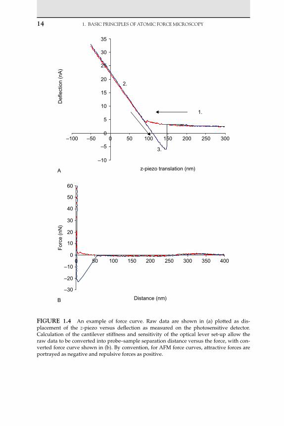
As the tip of the cantilever is brought into and out of contact with a surface, a force curve is generated, describing the cantilever deflection (or force) as a function of distance. A typical force curve is illustrated in Figure 1.4. Raw data are plotted as displacement of the z-piezo on the abscissa, whilst cantilever deflection is plotted as the signal on the pho-todetector (commonly either as voltage V or sometimes as current A) on the ordinate. As the cantilever begins its approach (described by the red trace), it is away from the surface and hence there is no detection of change in force (point 1 in the figure) – the cantilever is said to be at its ‘free level’, i.e. at this point there are no net forces acting on it (assum-ing that the probe is not travelling fast enough for hydrodynamic drag forces to have a significant effect). As the probe comes into close proxim-ity with the cantilever, long-range forces may cause interaction between the probe and the objective surface. Repulsive forces will cause the lever to deflect upwards and away from the surface, whereas attractive forces will deflect the lever downwards, towards the surface. If the gradient of attractive forces is less than the stiffness of the lever, then the probe will momentarily be deflected downwards, before re-equilibrating at its free level due to the restoring force stored in the lever. If the probe reaches a point where the gradient of attractive forces exceeds the stiffness of the cantilever, then the cantilever will be rapidly deflected downwards allowing the probe to touch the surface in a ‘snap-in’ or ‘jump-to- contact’. In the absence of attractive surface forces, this jump-to-contact will not be seen. When the cantilever makes hard contact with the sur-face, it is deflected upwards due to repulsion between electron shells of atoms in the opposing material surfaces, and a positive force is observed (point 2). The cantilever is then retracted and initially follows the path of the approach trace in the contact region. The cantilever often remains attached to the surface by adhesive forces which results in a downwards deflection of the cantilever as the probe retracts away from the surface, causing a hysteresis between the trace and the retrace. Eventually the separation force becomes sufficient to overcome the adhesion between the probe tip and the surface, and the cantilever snaps back to its initial free level position (point 3).
This behaviour results in a curve of deflection (measured as raw sig-nal) versus displacement of the piezo in the z-direction. When the surface being pressed against is hard and does not undergo significant deforma-tion, the z-movement will be equal to the deflection of the cantilever. As a
�4 1. BAsICPRINCIPLEsOFATOMICFORCEMICROsCOPy
fIgure �.4 An example of force curve. Raw data are shown in (a) plotted as dis-placement of the z-piezo versus deflection as measured on the photosensitive detector. Calculation of the cantilever stiffness and sensitivity of the optical lever set-up allow the raw data to be converted into probe–sample separation distance versus the force, with con-verted force curve shown in (b). By convention, for AFM force curves, attractive forces are portrayed as negative and repulsive forces as positive.
Distance (nm)
–30
–20
–10
0
10
20
30
40
50
60
0 50 100 150 200 250 300 350 400
For
ce (
nN)
B
–10
–5
0
5
10
15
20
25
30
35
–100 –50 0 50 100 150 200 250 300
z-piezo translation (nm)
Def
lect
ion
(nA
)
A
1.
2.
3.

1.5 THEAFMAsAFORCEsENsOR �5
consequence, the slope obtained from contact with an unyielding surface provides the sensitivity of the optical lever system. By dividing the raw deflection data by this sensitivity value, it can be converted into an actual deflection distance. This sensitivity value is essential for the calculation of force values from raw deflection data. This deflection value (distance) can also then be subtracted from the z-piezo displacement to give the actual distance travelled by the probe. An alternative method of finding the optical lever sensitivity without needing to make hard contact with the surface was suggested by Higgins et al. [94] (Section 1.4).
Within operational limits the AFM cantilever behaves as a linear, or ‘Hookean’, spring. As a result the magnitude of the deflection of the can-tilever can be used to calculate the force which is exerted on the cantile-ver using Hooke’s law:
F kx (1.1)
where F is force (N), x the deflection of the cantilever (m) and k the spring (or force) constant of the cantilever (N m1), which essentially represents the stiffness of the cantilever. This spring constant is dependent upon the physical properties of the lever. This is apparent from the following rela-tion, used to describe a rectangular, ‘diving board’ shaped lever as shown in 1. 5 [16, 95]:
k
Et wl
3
34 (1.2)
where E is the Young’s modulus of the lever and t, w and l the thickness, width and length of the lever, respectively. However, it must be borne in mind that none of the diving board levers are perfectly rectangular, due to shaping of the ends of the beams and imperfections in the manufactur-ing process. As a result this equation will give only an approximate value for the stiffness of a rectangular cantilever. In the next section the need for the methods used to effectively measure the stiffness of a cantilever to be used for force measurements, whether it is rectangular or V-shaped, and the reasons for variability in k between cantilevers are addressed in greater detail.
For different applications, cantilevers with different spring constants may be needed. For instance, for intermittent contact mode in air, par-ticularly stiff levers are needed to overcome capillary forces, whereas for measurement of weak interaction forces, very soft levers are needed for their increased force sensitivity. The most convenient ways of producing this variation are by altering the length and or thickness of levers during production in order to increase or decrease the lever stiffness.
�6 1. BAsICPRINCIPLEsOFATOMICFORCEMICROsCOPy
�.6 CalIbraTIon of afm mICroCanTIlevers
�.6.� Calibration of normal spring Constants
For the accurate measurement of forces, the spring constant of the can-tilever needs to be known. In particular, for forces normal to the surfaces of interest, this is the spring constant which governs the relationship between force and deflection in the z-direction, as opposed to the lateral and torsional spring constants (see Section 1.4.2). Although cantilevers are supplied with a manufacturers’ ‘nominal’ value, the actual value can vary to a high degree, mostly due to variations in the thickness of the levers and defects in the material of the cantilevers themselves. The cubic relationship between thickness and the spring constant seen in equation (1.2) means that small variations in thickness can cause significant varia-tions in k. Because of this variability, for force experiments the cantilevers to be used need to be calibrated to determine a more accurate value of k. There are now a large number of methods by which the spring constant can be calculated, each with their own advantages and disadvantages. Four of the most extensively used approaches are described later.
A number of methods exist which involve calculating spring constants based upon the dimensions and geometry of the lever. Whilst calcula-tions for rectangular cantilevers, such as in equation (1.2), are relatively straightforward, for V-shaped cantilevers, approximations are most often used based upon a simplification of their geometry, e.g. Sader approxi-mated a V-shaped cantilever to two parallel rectangular beams [96]. This resulted in the following equation to describe a V-shaped lever:
k
Et wl
wb
3
3
3
3
1
21
43 2cos ( cos )
(1.3)
where is the inside angle between the two arms of the V-shaped lever, w the width of each of the lever arms parallel to the base of the lever and b the outer width of the base of the lever (see Figure 1.5 for diagram-matic explanation of the dimensions). This equation, as well as equation (1.2), assumes that the point of loading of force on the cantilever will be at the very apex. As the probe tip itself, where the loading of force actu-ally occurs, is often sited a short distance from the very end, this needs to be taken into account. A simple correction may be applied based on the length of the lever and the distance of the probe from the end of the lever [96–98]:
k k l lc m ( / )∆ 3 (1.4)

1.6 CALIBRATIONOFAFMMICROCANTILEvERs �7
where km is the uncorrected calculated spring constant value, kc the cor-rected value and l the distance of the centre of the base of the probe from the apex of the lever.
The problem with calculating spring constants purely from the measured dimensions of the lever and nominal values for the Young’s modulus is pri-marily that during cantilever manufacture variability in the material proper-ties, particularly the Young’s modulus, of cantilevers can occur largely due to variations in the morphology of the silicon nitride [23]. In addition, accu-rate determination of lever thickness is not always very practicable. Making accurate measurements for every lever used in experiments by SEM is time consuming and not necessarily convenient. By measuring the resonance behaviour of cantilevers, variability in the material properties of the canti-levers can be at least to some extent taken into account. This leads to a more reliable calculation for the spring constant of a cantilever surrounded by a fluid environment, such as air, from the following relationship [99, 100]:
k b lQf i f f 0 1906 2 2. ( ) Γ (1.5)
where f is the density of the surrounding fluid; Q the quality factor (a measure of the sharpness of the resonance peak); i the imaginary com-ponent of the hydrodynamic function, dependent upon the Reynolds number of the fluid; and f the fundamental resonance frequency of the cantilever. Although this approach is reliable for calibrating rectangular levers, there are not currently any reliable approximations to allow this method to be used for the commonly used V-shaped cantilevers.
Another method, developed by Cleveland et al. [95], requires the attachment of known masses, such as tungsten spheres, to the end of the cantilever whilst monitoring the resultant resonant frequency change. Measuring the position of the fundamental resonance peak of the cantilever before and after the addition of the sphere allows the follow-ing relationship to be used to calculate the spring constant:
k
Mv v
( )( / ) ( / )
21 1
2
12
02π (1.6)
fIgure �.5 Diagram showing relevant dimen-sions on a beam-shaped AFM cantilever.
l
t
w

�8 1. BAsICPRINCIPLEsOFATOMICFORCEMICROsCOPy
where M is the added mass, k the cantilever spring constant and v0 and v1 the unloaded and loaded resonant frequencies.
Although this method can produce a value for the cantilever spring constant to a high degree of accuracy, there are some problems. Attaching the bead to the cantilever, especially if attached using glue, can be a destructive process, rendering the lever unusable for further experiments. This means that calibration must be carried out at the end of experimental measurements. However, with sufficient care spheres may be attached in air using capillary adhesion forces alone. In addition errors may occur from the incorrect placement of the sphere or uncer-tainties in the mass of the sphere. If the sphere is placed a short dis-tance away from the end of the lever, then the value obtained from this method will be high, as k is inversely proportional to the cube of the cantilever length l. Again, this can be simply accounted for by utilizing equation (1.4).
The masses of spheres ordinarily used in this technique are on the order of a nanogram, making accurate weighing problematic. As such, masses are generally estimated from the size and density of the spheres, which may in turn lead to measurement errors. To allow for this, measure-ments may be made using several spheres of different masses. A plot of M versus (2v1)2 can then be made, which will have a slope equal to the spring constant of the cantilever [95, 101]. The advantages of this method are that the measurements are independent of the cantilever geometry and material properties, and many commercially available AFMs have the capability to measure cantilever resonant frequencies.
Another technique commonly used to quantify cantilever spring constants is the so-called ‘thermal method’ devised by Hutter and Bechhoefer [102, 103]. Here the area of the fundamental resonant peak of the cantilever under ambient thermal excitation, when not in the pres-ence of a surface, can be used to directly calculate the spring constant of
the cantilever. The mean square deflection of the cantilever, x2 , due to
thermal fluctuations can be related to the spring constant thus, assuming an idealised spring behaviour:
kk T
xB
2 (1.7)
where kB and T are Boltzmann’s constant (1.38 1023 J K1) and abso-lute temperature, respectively, together representing the thermal energy of the system. Once other noise sources are subtracted from the back-ground, the area of the fundamental resonance peak will be equal to the mean square displacement. However, as the cantilever is not an ideal

1.6 CALIBRATIONOFAFMMICROCANTILEvERs ��
spring, equation (1.7) is insufficient to describe its behaviour, and a num-ber of other factors may need to be taken into account [103–107]:
k
s k TP
D lD l
B
0 8174 1 3 21 2
2 2. tan /
tan /cos
ϕϕ
ϕ
(1.8)
where D is the tip height, s the sensitivity (in V or A m1), and P the posi-tional noise power of the fundamental resonance peak (the area under the fundamental resonance peak in the power spectral density (PSD) curve), obtained from a plot of the thermal power spectrum. Thus, with a spectrum analyser and appropriate software available with a number of commercially available AFM instruments, spring constant calibration is relatively straightforward as well as being relatively non-destructive.
Higgins et al. [94] suggested a novel way of finding the optical lever sensitivity by combining this thermal method with those of Sader. By using Sader’s method to determine a spring constant for the cantile-ver, the method of Hutter and Bechhoefer could then be used to back- calculate the optical lever sensitivity without the need to make a hard con-tact with a stiff surface. This method is potentially of use where a hard contact is undesirable, for instance when the probe is chemically function-alised or when a particle made of some deformable material, which is likely to significantly deform under measurement stresses, is used as a probe.
A very simple and straightforward method of calibrating the cantilever spring constant is to press the cantilever to be calibrated against another, reference, cantilever of known k (Figure 1.6). This could be either a mac-roscopic lever [108] or another AFM microcantilever [109]. Reference cantilevers can be obtained either commercially or by using another cali-bration method or combination of other methods to determine k to a high precision. When the two levers are pressed together, the slope of the con-tact region on the force curve will be the result of the deflection of both levers. As a result, comparison of this slope with the slope obtained when
fIgure �.6 Diagram-matic representation of a V-shaped AFM cantilever.
w
b
t
α
w ′
ll ′
20 1. BAsICPRINCIPLEsOFATOMICFORCEMICROsCOPy
pressed against a hard surface, which will not appreciably deform under the pressure exerted upon it, will allow the calculation of the unknown spring constant, providing that the same optical lever set-up and hence its sensitivity remains unchanged between each set of measurements:
k kc refhard ref
ref
ϕcos
(1.9)
k kc refhard
ref
1
(1.10)
where kc and kref are the spring constants of the unknown and known reference levers, hard and ref the gradients of the contact regions of force curves against a hard surface and the reference lever, respectively, ϕ the angle between the two levers.
Typically levers are mounted onto the AFM with an in-built tilt angle of approximately 10–12°, which is liable to give a value of k varying from the true value by less than the experimental uncertainty. In addition, if care is taken to maintain the same angle between the lever and the experimental sample when calibrating the lever, then the apparent spring constant calcu-lated by this method will be identical to the effective spring constant. As such the term cos ϕ can be ignored (equation (1.10)). This is a quick and simple method to use and can be carried out where the instrumentation being used does not allow the measurement of the resonance spectrum of the cantilever.
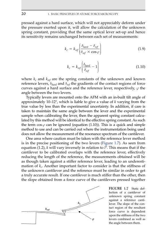
One area where caution must be taken with the reference lever method is in the precise positioning of the two levers (Figure 1.7). As seen from equation (1.2), k will vary inversely in relation to l3. This means that if the cantilever to be calibrated overlaps with the reference lever, effectively reducing the length of the reference, the measurements obtained will be as though taken against a stiffer reference lever, leading to an underesti-mation of kc. Another important factor to consider is that the stiffness of the unknown cantilever and the reference must be similar in order to get a truly accurate result. If one cantilever is much stiffer than the other, then the slope obtained from a force curve of the cantilevers pressed together
fIgure �.7 Static def- lection of a cantilever of unknown spring constant against a reference canti-lever. The slope of the con-tact region of the resultant force curve is dependent upon the stiffness of the two levers combined as well as the angle between them.
kref
kc
ϕ

1.6 CALIBRATIONOFAFMMICROCANTILEvERs 2�
will be dominated by the deflection of the softer lever. It has been sug-gested that one lever should not have a spring constant greater than the other by more than a factor of three [109] for this method to be effective.
This is only a selection of some of the more commonly used tech-niques. There are a large number of other methods used to determine spring constants of AFM cantilevers listed in the literature. These include, in no especial order, the measurement of the dynamic response of cantile-vers with colloidal spheres attached in a viscous fluid [110, 111]; calculat-ing k of levers on a chip, based on geometry, compared with a lever on the same chip calibrated by another method [97]; an alternative ‘thermal method’ with k calculated from the resonant frequency, Q factor and the squared resonance amplitude [112]; and measuring the static deflection of an AFM cantilever due to a known end-loaded mass [113].
�.6.2 Calibration of Torsional and lateral spring Constants
To extract quantitative data from measurements of lateral forces expe-rienced by the probe when scanning across a surface, such as in friction force microscopy, then the stiffness of the cantilever in the lateral or tor-sional mode needs to be ascertained. However, this is much less straight-forward than calibrating the normal spring constant of the lever. For frictional measurements, as well as knowledge of the normal and tor-sional spring constants, knowledge of the lateral response of the deflec-tion sensor and the geometry, height and material properties of the probe at the region of contact with the sample need to be ascertained.
At this point the difference between the torsional and lateral stiffnesses of the cantilevers must be made clear. The torsional spring constant k is the resistance to rotation along the major axis of the cantilever. The lateral spring constant klat on the contrary is the resistance of the lever to forces experi-enced laterally at the apex of the probe tip, producing a rotation at the base of the probe. The two are related by the following simple formula [114]:
k
khlat Φ
2 (1.11)
where h is the height of the probe (usually in the region of 3 μm for most imaging probes).
Sader described equations to calculate the approximate k for both beam-shaped and V-shaped cantilevers [115] from their geometries. Torsional stiffness for a beam-shaped cantilever is:
kEt wv l l
l lw
v
vw
l lφ
3
6 11
6 1
6 1( )( )
tanh ( )
( )+ −
∆
∆
∆
1
(1.12)
22 1. BAsICPRINCIPLEsOFATOMICFORCEMICROsCOPy
and for torsional forces experienced by a V-shaped cantilever:
kEt w
v lwb
wb
ll
blφ
3 2
3 11 2
22
38
1
1( )log
∆
bl
22
2
4
−1
(1.13)
where l is the distance of the base of the probe tip from the apex of the lever.
For relevant dimensions of the levers see Figures 1.5 and 1.6. In terms of measured interactions, klat can be defined in similar terms to Hooke’s law for the normal spring constant of the lever [73]:
F k xlat lat ∆ (1.14)
where Flat is the force experienced by the tip and x the lateral move-ment of the tip along the x-direction (i.e. at right angles to the major axis of the cantilever).
�.7 ColloId probes
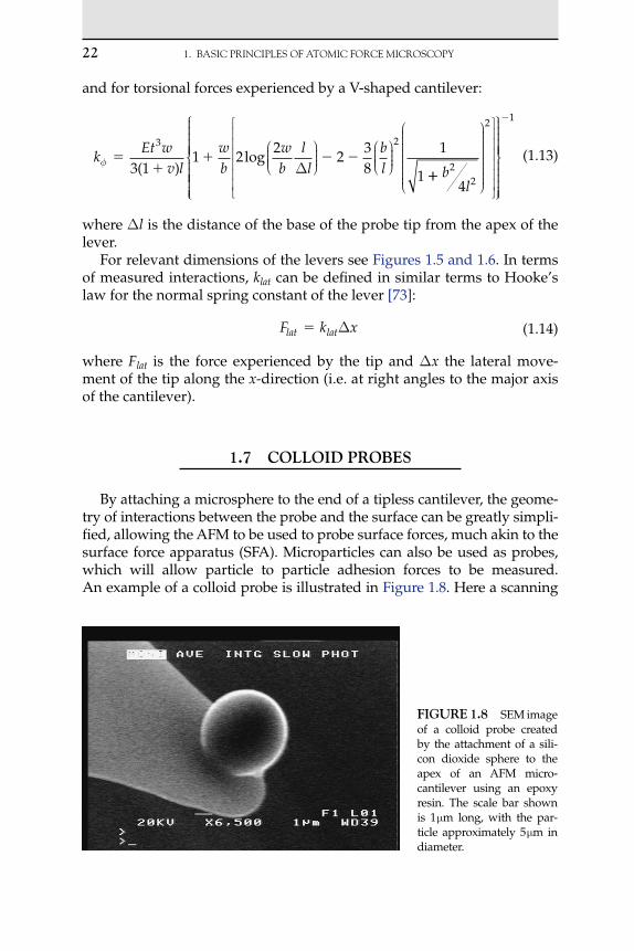
By attaching a microsphere to the end of a tipless cantilever, the geome-try of interactions between the probe and the surface can be greatly simpli-fied, allowing the AFM to be used to probe surface forces, much akin to the surface force apparatus (SFA). Microparticles can also be used as probes, which will allow particle to particle adhesion forces to be measured. An example of a colloid probe is illustrated in Figure 1.8. Here a scanning
fIgure �.8 SEM image of a colloid probe created by the attachment of a sili-con dioxide sphere to the apex of an AFM micro-cantilever using an epoxy resin. The scale bar shown is 1 m long, with the par-ticle approximately 5 m in diameter.
ABBREvIATIONsANdsyMBOLs 23
electron microscope (SEM) image shows a 5-μm diameter silica bead attached with glue close to the apex of a standard AFM microcantilever.
The first reported use of an AFM with a colloidal probe was by Ducker et al. [116, 117] who attached a 3.5-μm silica sphere to an AFM cantilever and used it to measure forces between the sphere and a silica surface as a function of electrolyte concentration and pH. Since then this technique has been used to probe the interaction forces between various materials and surfaces including silicates and other inorganic materials [80, 83, 117, 118], protein- and polymer-coated beads and surfaces [119–122], mem-brane-fouling materials and membranes [123], biological cells and sur-faces [124, 125]; between drug particles which are important in powder formulations [81, 84, 87]; and for probing the rheological properties of liquids [110, 126]. See Chapter 2 for more detail on the preparation of col-loid probes.
abbrevIaTIons and symbols
AFM Atomic force microscopy/microscopeb Outer width of the base of V-shaped cantilever mE Young’s modulus N m2
F Force normal to sample surface NFlat Lateral forces NJKR Johnson, Kendall and Roberts theoryk Spring constant of cantilever N m1
kB Boltzmann’s constant (1.38 1023) J K1
kc Corrected k N m1
klat Lateral spring constant N m1
km Uncorrected k N m1
kref Reference cantilever spring constant N m1
k Torsional spring constant N m1
l Cantilever length mM Mass added to cantilever kgP Positional noise power of fundamental resonant peakPDMS PolydimethylsiloxaneQ Quality factor of cantilever –SPM Scanning probe microscopySTM Scanning tunnelling microscopy/microscopet Cantilever thickness m

24 1. BAsICPRINCIPLEsOFATOMICFORCEMICROsCOPy
T Absolute temperature Kv0 Unloaded resonant frequency Hzv1 Loaded resonant frequency Hzw Cantilever width mx Deflection of cantilever m Inside angle of V-shaped cantilever °i Imaginary component of hydrodynamic function –hard Contact slope versus hard surface nm V1
ref Contact slope measured versus reference cantilever nm V1
f Density of surrounding fluid Pa sϕ Angle between cantilever and reference lever °f Fundamental resonant frequency of lever Hz
references [1] G. Binnig, C.F. Quate, C. Gerber, Atomic force microscope, Phys. Rev. Lett. 56 (9)
(1986) 930–933. [2] S. Alexander, L. Hellemans, O. Marti, J. Schneir, V. Elings, P.K. Hansma, M. Longmire,
J. Gurley, An atomic resolution atomic force microscope implemented using an optical lever, J. Appl. Phys. 65 (1) (1988) 164–167.
[3] G. Meyer, N.B. Amer, Novel optical approach to atomic force microscopy, Appl. Phys. Lett. 53 (12) (1988) 1045–1047.
[4] Y. Martin, C.C. Williams, H.K. Wickramasinghe, Atomic force microscope – force map-ping and profiling on a sub 100-Å scale, J. Appl. Phys. 61 (10) (1987) 4723–4729.
[5] R. Jumpertz, A.v.d. Hart, O. Ohlsson, F. Saurenbach, J. Schelten, Piezoresistive sensors on AFM cantilevers with atomic resolution, Microelectronic Engineering, 41/42 (1998) 441–444.
[6] P.A. Rasmussen, J. Thaysen, S. Bouwstra, A. Boisen, Modular design of AFM probe with sputtered silicon tip, Sensors Actuat. A 92 (2001) 96–101.
[7] M. Tortonese, R.C. Barrett, C.F. Quate, Atomic resolution with an atomic force micro-scope using piezoresistive detection, Appl. Phys. Lett. 62 (8) (1993) 834–836.
[8] T. Gotszalk, P. Grabiec, F. Shi, P. Dumania, P. Hudek, I.W. Rangelow, Fabrication of multipurpose AFM/SCM/SEP microprobe with integrated piezoresistive deflection sensor and isolated conductive tip, Microelectron. Eng. 41/42 (1998) 477–480.
[9] P.-F. Indermuhle, G. Schurmann, G.-A. Racine, N.F. De Rooij, Fabrication and char-acterization of cantilevers with integrated sharp tips and piezoelectric elements for actuation and detection for parallel applications, Sensors Actuat. A 60 (1997) 186–190.
[10] T. Itoh, T. Suga, Self-excited force-sensing microcantilevers with piezoelectric thin films for dynamic scanning force microscopy, Sensors Actuat. A 54 (1996) 477–481.
[11] C. Lee, T. Itoh, T. Suga, Self-excited piezoelectric PZT microcantilevers for dynamic SFM – with inherent sensing and actuating capabilities, Sensors Actuat. A 72 (1999) 179–188.
[12] Y. Su, A. Brunnschweiler, A.G.R. Evans, G. Ensell, Piezoresistive silicon V-AFM canti-levers for high-speed imaging, Sensors Actuat. A 76 (1999) 139–144.
[13] H. Takahashi, K. Ando, Y. Shirakawabe, Self-sensing piezoresistive cantilever and its magnetic force microscopy applications, Ultramicroscopy 91 (2002) 63–72.

REFERENCEs 25
[14] J. Thaysen, A. Boisen, O. Hansen, S. Bouwstra, Atomic force microscopy probe with piezoresiostive read-out and a highly symmetrical Wheatstone bridge arrangement, Sensors Actuat. A 83 (2000) 47–53.
[15] S. Akamine, R.C. Barrett, C.F. Quate, Improved atomic force microscope images using microcantilevers with sharp tips, Appl. Phys. Lett. 57 (3) (1990) 316–318.
[16] T.R. Albrecht, S. Akamine, T.E. Carver, C.F. Quate, Microfabrication of cantilever styli for the atomic force microscope, J. Vac. Sci. Technol. A 8 (4) (1990) 3386–3396.
[17] J. Brugger, R.A. Buser, N.F. de Rooij, Silicon cantilevers and tips for scanning force microscopy, Sensors Actuat. A 34 (1992) 193–200.
[18] C. Liu, R. Gamble, Mass-producible monolithic silicon probes for scanning probe microscopes, Sensors Actuat. A 71 (1998) 233–237.
[19] O. Wolter, T. Bayer, J. Greschner, Micromachined silicon sensors for scanning force microscopy, J. Vac. Sci. Technol. B 9 (2) (1990) 1353–1357.
[20] S. Hosaka, K. Etoh, A. Kikukawa, H. Koyanagi, K. Itoh, 6.6 MHz silicon AFM canti-lever for high-speed readout in AFM based recording, Microelectron. Eng. 46 (1999) 109–112.
[21] S. Habermehl, Stress relaxation in Si-rich silicon nitride thin films, J. Appl. Phys. 83 (9) (1998) 4672–4677.
[22] K.E. Peterson, Silicon as a mechanical material, Proc. IEEE 70 (5) (1982) 420–457. [23] A. Khan, J. Philip, P. Hess, Young’s modulus of silicon nitride used in scanning force
microscope cantilevers, J. Appl. Phys. 95 (4) (2004) 1667–1672. [24] J.J. Wortman, R.A. Evans, Young’s modulus, shear modulus, and Poisson’s ratio in
silicon and germanium, J. Appl. Phys. 36 (1) (1965) 153–156. [25] T. Hantschel, S. Slesazeck, P. Niedermann, P. Eyben, W. Vandervorst, Integrating
diamond pyramids into metal cantilevers and using them as electrical AFM probes, Microelectron. Eng. 57–58 (2001) 749–754.
[26] K. Unno, T. Shibata, E. Makino, Micromachining of diamond probes for atomic force microscopy applications, Sensors Actuat. A 88 (2001) 247–255.
[27] W. Kulisch, A. Malave, G. Lippold, W. Scholtz, C. Mihalcea, E. Oesterschulze, Fabrication of integrated diamond cantilevers with tips for SPM applications, Diamond Relat. Mater. 6 (1997) 906–911.
[28] T. Akiyama, U. Staufer, N.F. De Rooij, L. Howald, L. Scandella, Lithographically defined polymer tips for quartz tuning fork based scanning probe microscopes, Microelectron. Eng. 58-58 (2001) 769–773.
[29] R. Erlandsson, G. Hadziioannou, C.M. Mate, G.M. McClellamd, S. Chiang, Atomic scale friction between the muscovite mica cleavage plane and a tungsten tip, J. Chem. Phys. 89 (8) (1988) 5190–5192.
[30] C.M. Mate, G.M. McClellamd, R. Erlandsson, S. Chiang, Atomic-scale friction of a tungsten tip on a graphite surface, Phys. Rev. Lett. 59 (17) (1987) 1942–1946.
[31] Y. Miyahara, T. Fujii, S. Watanabe, A. Tonoli, S. Carabelli, H. Yamada, H. Bleuler, Lead zirconate titanate cantilever for non-contact atomic force microscopy, Appl. Surf. Sci. 140 (1999) 428–431.
[32] A.H. Sorenson, U. Hvid, M.W. Mortensen, K.A. Morch, Preparation of platinum/ iridium scanning probe microscopy tips, Rev. Sci. Instrum. 70 (7) (1999) 3059–3067.
[33] E.I. Givargizov, A.N. Stepanova, E.S. Mashkova, V.A. Molchanov, F. Shi, P. Hudek, I.W. Rangelow, Ultrasharp diamond coated silicon tips for scanning probe devices, Microelectron. Eng. 41/42 (1998) 499–502.
[34] E.I. Givargizov, A.N. Stepanova, L.N. Obelenskaya, E.S. Mashkova, V.A. Molchanov, M.E. Givargizov, I.W. Rangelow, Whisker probes, Ultramicroscopy 82 (2000) 57–61.
[35] S.S. Wong, E. Joselevich, A.T. Woolley, C.L. Cheung, C.M. Lieber, Covalently func-tionalized nanotubes as nanometre sized probes in chemistry and biology, Nature 394 (1998) 52–55.
26 1. BAsICPRINCIPLEsOFATOMICFORCEMICROsCOPy
[36] C.L. Cheung, J.H. Hafner, T.W. Odom, K. Kim, C.M. Lieber, Growth and fabrication with single-walled carbon nanotube probe microscopy tips, Appl. Phys. Lett. 76 (21) (2000) 3136–3138.
[37] H.J. Dai, J.H. Hafner, A.G. Rinzler, D.T. Colbert, R.E. Smalley, Nanotubes as nano-probes in scanning probe microscopy, Nature 384 (6605) (1996) 147–150.
[38] C.T. Gibson, S. Carnally, C.J. Roberts, Attachment of carbon nanotubes to atomic force microscope probes, Ultramicroscopy 107 (10–11) (2007) 1118–1122.
[39] J.H. Hafner, C.L. Cheung, C.M. Lieber, Growth of nanotubes for probe microscopy tips, Nature 398 (6730) (1999) 761–762.
[40] E. Bonnaccurso, G. Gillies, Revealing contamination on AFM cantilevers by micro-drops and microbubbles, Langmuir 20 (2004) 11824–11827.
[41] T. Thundat, X.-Y. Zheng, G.Y. Chen, S.L. Sharp, R.J. Warmack, L.J. Schowalter, Characterization of atomic force microscope tips by adhesion force measurements, Appl. Phys. Lett. 63 (15) (1993) 2150–2152.
[42] L. Sirghi, O. Kylian, G. Ceccone, F. Rossi, Cleaning and hydrophobization of atomic force microscopy silicon probes, J. Phys. Chem. B 110 (2006) 25975–25981.
[43] Y.-S. Lo, N.D. Huefner, W.S. Chan, P. Dryden, B. Hagenhoff, T.P. Beebe Jr., Organic and inorganic contamination on commercial AFM cantilevers, Langmuir 15 (1999) 6522–6526.
[44] S.W. King, R.J. Nemanich, R.F. Davis, Wet chemical processing of (0001)Si 6H-SiC hydrophobic and hydrophilic surfaces, J. Electrochem. Soc. 146 (5) (1999) 1910– 1917.
[45] D.A. Dobbs, R.G. Bergman, K.H. Theopold, Piranha solution explosion, Chem. Eng. News 68 (17) (1990) 2.
[46] C.V. Erickson, Piranha solution explosions, Chem. Eng. News 68 (33) (1990) 2. [47] T. Arai, M. Tomitori, Removal of contamination and oxide layers from UHV-AFM tips,
Appl. Phys. A 66 (1998) S319–S323. [48] K. Choi, T.-J. Eom, C. Lee, Comparison of the removal efficiency for organic con-
taminants on silicon wafers stored in plastic boxes between UV/O3 and ECR oxygen plasma cleaning methods, Thin Solid Films 435 (2003) 227–231.
[49] E. Bonaccurso, G. Gillies, Revealing contamination on AFM cantilevers by microdrops and microbubbles, Langmuir 20 (2004) 11824–11827.
[50] R. Luginbuhl, A. Szuchmacher, M.D. Garrison, J.-B. Lhoest, R.M. Overney, B.D. Ratner, Comprehensive surface analysis of hydrophobically functionalized SFM tips, Ultramicroscopy 82 (2000) 171–179.
[51] L. Montellius, J.O. Tegenfeldt, Direct observation of the tip shape in scanning probe microscopy, Appl. Phys. Lett. 62 (21) (1993) 2628–2630.
[52] E.J. van Loenen, D. Dijkamp, A.J. Hoeven, J.M. Lenssink, J. Dieleman, Evidence for tip imaging in scanning tunneling microscopy, Appl. Phys. Lett. 56 (18) (1990) 1755–1757.
[53] H.G. Hansma, R.L. Sinsheimer, J. Groppe, T.C. Bruice, V. Elings, M. Bezanilla, I.A. Mastrangelo, P.V.C. Hough, P.K. Hansma, Recent advances in atomic-force micro-scopy of DNA, Scanning 15 (5) (1993) 296–299.
[54] H.G. Hansma, J.P. Cleveland, M. Radmacher, D.A. Walters, P.E. Hillner, M. Bezanilla, M. Fritz, D. Vie, H.G. Hansma, C.B. Prater, J. Massie, L. Fukunaga, J. Gurley, V. Elings, Tapping mode atomic force microscopy in liquids, Appl. Phys. Lett. 64 (13) (1994) 1738–1740.
[55] Q. Zhong, D. Inniss, K. Kjoller, V. Elings, Fractured polymer/silica fiber surface stud-ied by tapping mode atomic force microscopy, Surf. Sci. Lett. (1993) L688–L692.
[56] I. Schmitz, M. Schreiner, G. Friedbacher, M. Grasserbauer, Phase imaging as an exten-sion to tapping mode AFM for the identification of material properties on humidity sensitive surfaces, Appl. Surf. Sci. 115 (1997) 190–198.
[57] R.S. McLean, B.B. Sauer, Tapping mode AFM studies using phase detection for res-olution of nanophases in segmented polyurethanes and other block copolymers, Macromolecules 30 (1997) 8314–8317.

REFERENCEs 27
[58] J. Loos, The art of SPM: scanning probe microscopy in materials science, Adv. Mater. 17 (2005) 1821–1833.
[59] R. Lüthi, E. Meyer, L. Howald, H. Haefke, D. Asnselmetti, M. Dreier, M. Rüetschi, T. Bonner, R.M. Overney, J. Frommer, H.-J. Güntherodt, Progress in noncontact dynamic force microscopy, J. Vac. Sci. Technol. B 12 (3) (1994) 1673–1676.
[60] M. Radmacher, M. Fritz, J.P. Cleveland, D.A. Walters, P.K. Hansma, Imaging adhesion forces and elasticity of lysozyme adsorbed on mica with the atomic force microscope, Langmuir 10 (1994) 3809–3814.
[61] N. Chaiyut, T. Amornsakchai, S. Thanawan, Force volume imaging of defects in highly drawn high-density polyethylene, Polym. Test. 26 (2007) 396–401.
[62] C. Rotsch, M. Radmacher, Mapping local electrostatic forces with the atomic force microscope, Langmuir 13 (1997) 2825–2832.
[63] H. Hillborg, N. Tomczak, A. Olah, H. Schonherr, G.J. Vancso, Nanoscale hydropho-bic recovery: a chemical force microscopy study of UV/ozone-treated cross-linked poly(dimethylsiloxan), Langmuir 20 (2004) 785–794.
[64] H. Schonherr, C.L. Feng, N. Tomczak, G.J. Vancso, Compositional mapping of poly-mer surfaces by chemical force microscopy down to the nanometer scale: reactions in block copolymer microdomains, Macromol. Symp. 230 (2005) 149–157.
[65] E. A-Hassan, W.F. Heinz, M.D. Antonik, N.P. D’Costa, S. Nageswaran, C.-A. Schoenenberger, J.H. Hoh, Relative microelastic mapping of living cells by atomic force microscopy, Biophy. J. 74 (3) (1998) 1564–1578.
[66] M. Fritz, M. Radmacher, N. Peterson, H.E. Gaub, Visualization and identification of intracellular structures by force, modulation microscopy and drug induced degrada-tion, J. Vac. Sci. Technol. B 12 (3) (1994) 1526–1529.
[67] J.S. Jourdan, S.J. Cruchon-Dupeyrat, Y. Huan, P.K. Kuo, G.Y. Liu, Imaging nanoscopic elasticity of thin film materials by atomic force microscopy: effects of force modula-tion frequency and amplitude, Langmuir 15 (1999) 6495–6504.
[68] J.A. Otero, J.M. Lena, P. Pradanos, F. Tejerina, A. Hernandez, Characterisation of nano-filtration membranes. Structural analysis by the DSP model and microscopical tech-niques, J. Membr. Sci. 279 (2006) 410–417.
[69] W.J. Price, P.K. Kuo, T.R. Lee, R. Colorado Jr., Z.C. Ying, G.Y. Liu, Probing the local structure and mechanical response of nanostructures using force modulation and nanofabrication, Langmuir 21 (2005) 5422–5428.
[70] W.J. Price, S.A. Leigh, S.M. Hsu, T.E. Patten, G. Liu, Measuring the size dependence of Young’s modulus using force modulation atomic force microscopy, J. Phys. Chem. A 110 (2006) 1382–1388.
[71] R.W. Carpick, D.F. Ogletree, M. Salmeron, Lateral stiffness: a new nanomechanical measurement for the determination of shear strengths with friction force microscopy, Appl. Phys. Lett. 70 (1997) 1548–1550.
[72] C.T. Gibson, G.S. Watson, S. Myhra, Lateral force microscopy, Wear 213 (1997) 72–79. [73] M.A. Lantz, S.J. O’Shea, A.C.F. Hoole, M.E. Welland, Lateral stiffness of the tip and tip-
sample contact in frictional force microscopy, Appl. Phys. Lett. 70 (8) (1997) 970–972. [74] E. Tocha, H. Schonherr, G.J. Vancso, Quantitative nanotribology by AFM: a novel uni-
versal calibration platform, Langmuir 22 (2006) 2340–2350. [75] S.K. Kaliapan, B. Capella, Temperature dependent elastic–plastic behaviour of poly-
styrene studied using AFM force distance curves, Polymer 46 (2005) 11416–11423. [76] J. Domke, M. Radmach, Measuring the elastic properties of thin polymer films with
the atomic force microscope, Langmuir 14 (1998) 3320–3325. [77] C. Plassard, E. Lesniewska, I. Pochard, A. Nonat, Investigation of the surface structure
and elastic properties of calcium silicate hydrates at the nanoscale, Ultramicroscopy 100 (2004) 331–338.
[78] A. Vinckier, I. Heyvaert, A. D’Hoore, T. McKittrick, C. Van Haesendonck, Y. Engelboghs, L. Hellemans, Immobilizing and imaging microtubules by atomic force microscopy, Ultramicroscopy 57 (1995) 337–343.

28 1. BAsICPRINCIPLEsOFATOMICFORCEMICROsCOPy
[79] I. Dulinska, M. Targosz, W. Strojny, M. Lekka, P. Czuba, W. Balwierz, M. Szymonski, Stiffness of normal and pathological erythrocytes studied by means of atomic force microscopy, J. Biochem. Biophys. Meth. 66 (2006) 1–11.
[80] A.L. Weisenhorn, P. Maivald, H.-J. Butt, P.K. Hansma, Measuring adhesion, attraction and repulsion between surfaces in liquids with an atomic force microscope, Phys. Rev. B 45 (19) (1992) 11226–11233.
[81] C.J. Roberts, What can we learn from atomic force microscopy adhesion measure-ments with single drug particles?, Eur. J. Pharm. Sci. 24 (2005) 153–157.
[82] M. Kapple, H.-J. Butt, The colloidal probe technique and its application to adhesion force measurements, Part. Part. Syst. Charact. 19 (2002) 129–143.
[83] W.R. Bowen, N. Hilal, R.W. Lovitt, C.J. Wright, An atomic force microscopy study of the adhesion of a silica sphere to a silica surface – effects of surface cleaning, Colloids Surf. A: Physicochem Eng. Aspects 157 (1999) 117–125.
[84] J.K. Eve, N. Patel, S.Y. Luk, S.J. Ebbens, C.J. Roberts, A study of single drug particle adhesion interactions using atomic force microscopy, Int. J. Pharm. 238 (2002) 17–27.
[85] L. Xu, B.E. Logan, Analysis of bacterial adhesion using a gradient force analysis method and colloid probe microscopy, Langmuir 20 (2004) 8817–8822.
[86] N.A. Burnham, D.D. Dominguez, R.L. Mowery, R.J. Colton, Probing the surface forces of monolayer films with an atomic force microscope, Phys. Rev. Lett. 64 (16) (1990) 1931–1934.
[87] M. Davies, A. Brindley, X. Chen, M. Marlow, S.W. Doughty, I. Shrubb, C.J. Roberts, Characterization of drug particle surface energetics and Young’s modulus by atomic force microscopy, Pharm. Res. 22 (7) (2005) 1158–1166.
[88] G. Gillies, M. Kapple, H.-J. Butt, Surface and capillary forces encountered by zinc sulfide microspheres in aqueous electrolyte, Langmuir 21 (2005) 5882–5886.
[89] P.G. Hartley, F. Grieser, P. Mulvaney, G.W. Stevens, Surface forces and deformation at the oil–water interface probed using AFM force measurement, Langmuir 15 (1999) 7282–7289.
[90] S. Allen, X. Chen, J. Davies, M.D. Davies, A.C. Dawkes, J.C. Edwards, C.J. Roberts, J. Sefton, S.J.B. Tendler, P.M. Williams, Detection of antigen–antibody binding events with the atomic force microscope, Biochemistry 36 (1997) 7457–7463.
[91] R.B. Best, D.J. Brockwell, J.L. Toca-Herrerra, A.W. Blake, D.A. Smith, S.E. Radford, J. Clarke, Force mode atomic force microscopy as a tool for protein folding studies, Anal. Chim. Acta 479 (2003) 87–105.
[92] J. Clarke, P.M. Williams, Unfolding induced by mechanical force, in: J. Buchner and T. Kiefhaber (Ed.), Protein Folding Handbook, Part 1, Wiley-VCH, 2005, pp. 1111–1142.
[93] M. Rief, M. Gautel, F. Oesterhelt, J.M. Fernandez, H.E. Gaub, Reversible unfolding of individual titin immunoglobulin domains by AFM, Science 276 (1997) 1109–1113.
[94] M.J. Higgins, R. Proksch, J.E. Sader, M. Polcik, S. McEndoo, J.P. Cleveland, S.P. Jarvis, Noninvasive determination of optical lever sensitivity in atomic force microscopy, Rev. Sci. Instrum. 77 (2006) 013701.
[95] J.P. Cleveland, S. Manne, D. Bocek, P.K. Hansma, A nondestructive method for deter-mining the spring constant of cantilevers for scanning force microscopy, Rev. Sci. Instrum. 64 (2) (1993) 403–405.
[96] J.E. Sader, Parallel beam approximation for v-shaped atomic force microscopy canti-levers, Rev. Sci. Instrum. 66 (9) (1995) 4583–4586.
[97] C.T. Gibson, D.J. Johnson, C. Anderson, C. Abell, T. Rayment, Method to determine the spring constant of atomic force microscope cantilevers, Rev. Sci. Instrum. 75 (2) (2004) 565–567.
[98] J.E. Sader, I. Larson, P. Mulvaney, L.R. White, Method for the calibration of atomic force microscopy cantilevers, Rev. Sci. Instrum. 66 (7) (1995) 3789–3798.
[99] J.E. Sader, Frequency response of cantilever beams immersed in viscous fluids with applications to the atomic force microscope, J. Appl. Phys. 84 (1) (1998) 64–76.

REFERENCEs 2�
[100] J.E. Sader, J.W.N. Chon, P. Mulvaney, Calibration of rectangular atomic force micro-scopy cantilevers, Rev. Sci. Instrum. 70 (10) (1999) 3967–3969.
[101] J. Ralston, I. Larson, M.W. Rutland, A.A. Feiler, M. Kleijn, Atomic force microscopy and direct surface force measurements (IUPAC technical report), Pure Appl. Chem. 77 (2005) 2149–2170.
[102] L. Hutter, J. Bechhoefer, Calibration of atomic force microscope tips, Rev. Sci. Instrum. 64 (7) (1993) 1868–1873.
[103] R. Levy, M. Maaloum, Measuring the spring constant of atomic force microscope can-tilevers: thermal fluctuations and other methods, Nanotechnology 13 (2002) 33–37.
[104] H.-J. Butt, M. Jaschke, Calculation of thermal noise in atomic force microscopy, Nanotechnology 6 (1995) 1–7.
[105] J.L. Hutter, Comment on tilt of atomic force microscope cantilevers: effect on spring constant and adhesion measurements, Langmuir 21 (2005) 2630–2632.
[106] R.W. Stark, T. Drobek, W.M. Heckl, Thermomechanical noise of a free v shaped canti-lever for atomic force microscopy, Ultramicroscopy 86 (2001) 207–215.
[107] D.A. Walters, J.P. Cleveland, N.H. Thomson, P.K. Hansma, M.A. Wendman, G. Gurley, V. Elings, Short cantilevers for atomic force microscopy, Rev. Sci. Instrum. 67 (10) (1996) 3583–3590.
[108] A. Torii, M. Sasaki, K. Hane, S. Okuma, A method for determining the spring con-stant of cantilevers for atomic force microscopy, Meas. Sci. Technol. 7 (1996) 179–184.
[109] C.T. Gibson, G.S. Watson, S. Myra, Determination of the spring constants of probes for force microscopy/spectroscopy, Nanotechnology 7 (1996) 259–262.
[110] S.M. Notley, S. Biggs, V.S.J. Craig, Calibration of colloid probe cantilevers using the dynamic viscous response of a confined liquid, Rev. Sci. Instrum. 74 (9) (2003) 4026–4032.
[111] V.S.J. Craig, C. Neto, In situ calibration of colloid probe cantilevers in force micro-scopy: hydrodynamic drag on a sphere approaching a wall, Langmuir 17 (2001) 6018–6022.
[112] N.A. Burnham, X. Chen, C.S. Hodges, G.A. Matei, E.J. Thoreson, C.J. Roberts, M.C. Davies, S.J.B. Tendler, Comparison of calibration methods for atomic-force microscopy cantilevers, Nanotechnology 14 (2003) 1–6.
[113] T.J. Senden, W.A. Ducker, Experimental determination of spring constants in atomic force microscopy, Langmuir 10 (1994) 1003–1004.
[114] J.M. Neumeister, W.A. Ducker, Lateral, normal and longitudinal spring constants of atomic force microscopy cantilevers, Rev. Sci. Instrum. 65-8 (1994) 2257–2531.
[115] J.E. Sader, Susceptibility of atomic force microscope cantilevers to lateral forces, Rev. Sci. Instrum. 74 (4) (2003) 2438–2443.
[116] W.A. Ducker, T.J. Senden, R.M. Pashley, Direct measurement of colloidal forces using an atomic force microscope, Nature 353 (1991) 239–241.
[117] W.A. Ducker, T.J. Senden, Measurement of forces in liquids using a force microscope, Langmuir 8 (7) (1992) 1831–1836.
[118] M. Götzinger, W. Peukert, Dispersive forces of particle–surface interactions: direct AFM measurements and modelling, Powder Technol. 130 (2003) 102–103.
[119] X. Li-Chong, B.E. Logan, Interaction forces between colloids and protein-coated sur-faces using an atomic force microscope, Environ. Sci. Technol. 39 (2005) 3592–3600.
[120] G. Gillies, C.A. Prestidge, Colloid probe AFM investigation of the influence of crosslinking on the interaction behaviour and nano-rheology of colloidal droplets, Langmuir 21 (2005) 12342–12347.
[121] M. Reitsma, V. Craig, S. Biggs, Elasto-plastic and visco-elastic deformations of a pol-ymer sphere measured using colloid probe and scanning electron microscopy, Int. J. Adhesion Adhesives 20 (2000) 445–448.
[122] L.B.R. Castro, M. Kapple, D.F.S. Petri, Adhesion forces between hybrid colloidal par-ticles and concavilin A, Langmuir 22 (2006) 3757–3762.

30 1. BAsICPRINCIPLEsOFATOMICFORCEMICROsCOPy
[123] N. Hilal, W.R. Bowen, Atomic force microscopy study of the rejection of colloids by membrane pores, Desalination 150 (2002) 289–295.
[124] W.R. Bowen, N. Hilal, R.W. Lovitt, C.J. Wright, Direct measurement of the force of adhesion of a single biological cell using an atomic force microscope, Colloids Surf. A: Physiochem. Eng. Aspects 136 (1998) 231–234.
[125] X. Li, B.E. Logan, Analysis of bacterial adhesion using a gradient force analysis method and colloid probe atomic force microscopy, Langmuir 20 (2004) 8817–8822.
[126] M.S. Barrow, W.S. Bowen, N. Hilal, A. Al-Hussany, P.R. Williams, R.L. Williams, C.J. Wright, A study of the tensile properties of liquids in confined spaces using an atomic force microscope, Proc. R. Soc. Lond. A 459 (2003) 2885–2908.

Atomic Force Microscopy in Process Engineering ©2009,ElsevierLtd31
C H A P T E R
O U T L I N E
2.1 Introduction 32
2.2 Colloid Probes 32
2.3 Interaction Forces 352.3.1 van der Waals Forces 352.3.2 Electrical Double Layer Forces 442.3.3 DLVO Theory 532.3.4 Solvation Forces 582.3.5 Steric Interaction Forces 622.3.6 Hydrophobic Interaction Forces 632.3.7 Effect of Hydrodynamic Drag on AFM Force Measurements 66
2.4 Adhesion Forces Measured by AFM 672.4.1 Contact Mechanics and Adhesion 67
2.5 Effect of Roughness on Measured Adhesion and Surface Forces 70
Abbreviations and Symbols 70
Greek Symbols 73References 74
MeasurementofParticleandSurfaceInteractionsUsingForceMicroscopy
Nidal Hilal, Daniel Johnson, W. Richard Bowen and Paul M. Williams
2

32 2. MEASUREMENTOFPARTICLEANdSURFACEINTERACTIONS
2.1 IntRoduCtIon
In Chapter 1, discussion was made of the application of the AFM to the measurement of forces. In this chapter, we will describe the use of the AFM to quantitatively measure surface forces arising from the interac-tions between particles and between particles and surfaces. These forces are of particular interest in the study of colloidal dispersions, where the strength of interactions between particles governs the properties of the dispersion overall.
Most traditional methods used to study colloidal dispersions are ensemble techniques, where the interactions of a large number of particles are measured simultaneously. The advantage with the AFM is the ability to make measurements on the single-particle level and to measure forces, and hence interaction energies, with respect to intersurface distances. Depending upon the experimental set-up being employed, a number of different interactions may be measured, either separately or simultane-ously, including long-range forces such as van der Waals and electri-cal double layer forces, hydrophobic interactions, solvation forces, steric interactions, hydrodynamic drag forces as well as adhesion. In this chap-ter, the forces that are likely to be encountered when measuring interac-tions between particles and between particles and surfaces whilst using the AFM are described, with examples of the measurements extant in the literature being included. It is hoped that this chapter will serve as a use-ful and practical guide to anyone who is undertaking such measurements.
2.2 ColloId PRobES
By replacing the pyramidal or conical probe usually present on an AFM cantilever with a microsphere, the geometry of interactions between the probe and surface can be greatly simplified, allowing the AFM to be used to probe surface forces, much akin to the surface force apparatus (SFA). Microparticles can also be used as probes, which will allow particle-to-particle adhesion forces to be measured. An example of a colloid probe is shown in Figure 2.1. Here, a scanning electron microscope (SEM) image shows a 5 m diameter silica bead attached with glue close to the apex of a standard AFM microcantilever.
As the size of a spherical colloid probe is increased, the potential area of contact will also increase in proportion. For two spheres in close prox-imity, the force as a function of distance D is:
F D
R RR R
W D( ) ( )
2 1 2
1 2π
(2.1)

2.2 COLLOIdPROBES 33
where R1 and R2 are the radii of the two spheres and W(D) is the interac-tion energy per unit area as a function of distance [1, 2]. This relation-ship is referred to as the Derjaguin approximation. In the case of a sphere approaching a flat surface (or where one sphere is much greater in size than the other), this is further simplified to create:
F D R W D( ) ( ) 2 1π (2.2)
Note that the forces of interaction are proportional to the radius or radii of the interacting spheres. For this reason, it is typical in colloidal probe measurements to normalise forces by dividing by the radius of curvature of the probe. This generally leads to forces being measured in units of the form of mN m1. It should be noted that one of the assumptions on which the Derjaguin approximation is based is that the range of the interaction forces is much less than the radii of the interacting spheres. For small spheres with radii in the nanometre range, this approximation is likely to be invalid, a situation that has been recently experimentally verified by carrying out measurements using AFM tips terminated with particles with radii of 10 and 20 nm [3]. Dividing the forces by the particle radii was insufficient to superimpose the force traces obtained with these particles.
Colloidal probes are most commonly prepared by attaching the par-ticle to the apex of the AFM cantilever with an appropriate glue using a
FIGuRE 2.1 SEM image of a colloid probe created by the attachment of a glass sphere to the apex of an AFM microcantilever using an epoxy resin. The scale bar shown is 5 m long, with the particle approximately 7.5 m in diameter.

34 2. MEASUREMENTOFPARTICLEANdSURFACEINTERACTIONS
micromanipulator set-up, although where materials allow, sintering may be used, such as with polystyrene beads. Figure 2.2 shows a typical microma-nipulator set-up, utilised in the preparation of colloid probes. This consists of a micromanipulator platform positioned underneath an optical micro-scope, and connected to an electronic control unit. Colloidal particles are placed upside down on a cleaned microscope slide, where they adhere via capillary forces. At one end of the slide is placed a thin smear of an appro-priate adhesive. The AFM cantilever is allowed to come into contact with the glue, with care being taken to minimise the amount of glue present. Too much glue may cause problems with contamination. Any excess can be wiped off by scraping the cantilever carefully on a clean area of the slide. The stage is then moved until a suitable particle is located. The cantilever plus glue is then allowed to come into contact with the particle, removing it from the surface of the slide. The glue is allowed to set and the probe is then ready for use. An alternative method also used is to place a drop of glue on the end of the cantilever using a fine wire. Another wire is then used to pick up a particle using capillary adhesion and then place it on the glued end of the lever [4].
AD
A
E
B
C
FIGuRE 2.2 Illustration of a typical micromanipulator set-up. It consists of a movable stage (A) mounted below an optical microscope (B). Inset into the top-left corner is a close-up of the stage. Movement of the stage can be controlled via an electronic control console (C), shown here on the left. Cantilever, particle interaction can also be monitored via a dig-ital video camera (D) mounted on the microscope. The AFM cantilever is introduced to the underneath of a microscope slide mounted on the stage from the left, where it is allowed to come into contact with glue and particles attached to the slide. Fine control of the cantilev-er’s movement is attained via the manipulator joystick and vertical drive (E). On the moni-tor, a V-shaped AFM cantilever is visible. The picture was taken in the laboratory of the Department of Chemical and Environmental Engineering, University of Nottingham.

2.3 INTERACTIONFORCES 35
2.3 IntERACtIon FoRCES
2.3.1 van der Waals Forces
In the nineteenth century, J. D. van der Waals derived an equation of state to account for deviations in the observed behaviour of gases from the ideal gas law, pV nRT:
p
n a
VV nb nRTVW
VW 2
2
( )
(2.3)
where p is the pressure, V is the volume of the container, n is the number of gas molecules in moles, R is the gas constant and T is the temperature. This equation contained two new terms to account for deviations from ideal behaviour, which can be determined experimentally and which vary between different types of molecule; a vw, which accounts for attractive forces between the molecules and b vw, which accounts for the volume of space occupied by the gas molecules and from which other molecules are excluded. This exclusion leads to repulsive forces at short ranges, due to the Pauli exclusion principle. Whilst there is a wide range of interactions that may occur between atoms, molecules and materials made from them, the term ‘van der Waals forces’ has been applied to a set of attractive forces that have their origin in interactions between dipoles, both permanent and tem-porarily induced, present in atoms and molecules. They can be divided into three types depending upon the precise nature of the interaction: dipole-dipole interactions (Keesom forces); dipole-induced dipole interac-tions (Debye forces) and interactions between dipoles induced on oppos-ing atoms or molecules (London or dispersive forces), and thus all are of an electrostatic origin. The Keesom and Debye forces act between polar mol-ecules. However, the London dispersive forces may arise between neutral atoms and are thus potentially present in all interactions between materi-als. All of these forces have interaction potentials of the form:
w
C
r
C C C
rr
T K D L( )
( )
6 6
(2.4)
where w(r) is the interaction potential, Ct is the constant of the interaction and r is the closest separation distance between molecules – subscripts K, D and L denote Keesom, Debye and London interactions respectively. When reading the literature, it is important to bear in mind which forces are being referred to by the term van der Waals forces. Some authors include all three of the types of dipole interactions mentioned here as van der Waals forces, whilst other authors specifically only mean the dispersion component of the interaction.
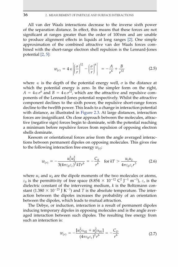
36 2. MEASUREMENTOFPARTICLEANdSURFACEINTERACTIONS
All van der Waals interactions decrease to the inverse sixth power of the separation distance. In effect, this means that these forces are not significant at ranges greater than the order of 100 nm and are unable to produce alignment effects in liquids at long ranges [2]. One simple approximation of the combined attractive van der Waals forces com-bined with the short-range electron shell repulsion is the Lennard-Jones potential [2, 5]:
w
r rAr
Br
r( ) 412 6
6 12
(2.5)
where is the depth of the potential energy well, is the distance at which the potential energy is zero. In the simpler form on the right, A 46 and B 412, which are the attractive and repulsive com-ponents of the Lennard-Jones potential respectively. Whilst the attractive component declines to the sixth power, the repulsive short-range forces decline to the twelfth power. This leads to a change in interaction potential with distance, as illustrated in Figure 2.3. At large distances, interaction forces are insignificant. On close approach between the molecules, attrac-tive (negative sign) forces begin to dominate, with the potential reaching a minimum before repulsive forces from repulsion of opposing electron shells dominate.
Keesom or orientational forces arise from the angle averaged interac-tions between permanent dipoles on opposing molecules. This gives rise to the following interaction free energy w(r):
w
u u
kTr
C
rkT
u u
rr
r
K
r( ) ( )
12
22
02 6 6
1 2
033 4 4πε ε πε ε
for
(2.6)
where u1 and u2 are the dipole moments of the two molecules or atoms, ε0 is the permittivity of free space (8.854 1012 C2 J1 m1), εr is the dielectric constant of the intervening medium, k is the Boltzmann con-stant (1.380 1023 J K1) and T is the absolute temperature. The inter-action between the dipoles increases the probability of an orientation between the dipoles, which leads to mutual attraction.
The Debye, or induction, interaction is a result of permanent dipoles inducing temporary dipoles in opposing molecules and is the angle aver-aged interaction between such dipoles. The resulting free energy from such an interaction is:
w
u u
r
C
rr
r
D( )
[ ]( )
12
02 22
01
02 6 64
α πε ε
(2.7)
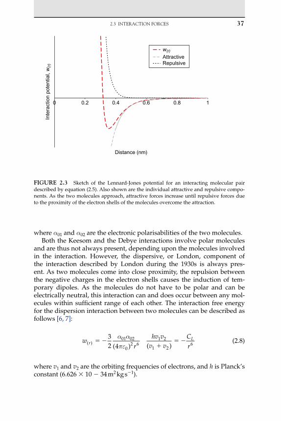
where 01 and 02 are the electronic polarisabilities of the two molecules.Both the Keesom and the Debye interactions involve polar molecules
and are thus not always present, depending upon the molecules involved in the interaction. However, the dispersive, or London, component of the interaction described by London during the 1930s is always pres-ent. As two molecules come into close proximity, the repulsion between the negative charges in the electron shells causes the induction of tem-porary dipoles. As the molecules do not have to be polar and can be electrically neutral, this interaction can and does occur between any mol-ecules within sufficient range of each other. The interaction free energy for the dispersion interaction between two molecules can be described as follows [6, 7]:
w
r
hv vv v
C
rr
L( ) ( ) ( )
32 4
01 02
02 6
1 2
1 26
πε
(2.8)
where v1 and v2 are the orbiting frequencies of electrons, and h is Planck’s constant (6.626 10 34 m2 kg s1).
w(r)
AttractiveRepulsive
0.2 0.4 0.8 10
Distance (nm)
Inte
ract
ion
pote
ntia
l, w
(r)
0.6
FIGuRE 2.3 Sketch of the Lennard-Jones potential for an interacting molecular pair described by equation (2.5). Also shown are the individual attractive and repulsive compo-nents. As the two molecules approach, attractive forces increase until repulsive forces due to the proximity of the electron shells of the molecules overcome the attraction.
2.3 INTERACTIONFORCES 37

38 2. MEASUREMENTOFPARTICLEANdSURFACEINTERACTIONS
2.3.1.1 van der Waals Forces Between Bulk MaterialsFor the useful estimation or measurement of van der Waals interaction
forces between colloidal particles and/or surfaces, the theory outlined in the previous section needs to be extrapolated to describe the behav-iour between materials rather than purely between individual atoms or molecules. A molecule at the surface of a particle in close proximity to another will interact with its neighbouring molecules, with molecules on the opposing particle as well as with the constituent molecules of the intervening medium. The summation of all the pair potentials interact-ing between macroscopic bodies results in forces that decay much more slowly with distance than is the case for single molecular interactions [2].
The effect of the dispersion force was investigated theoretically by Hamaker [8] and de Boer [9]. For interactions between spherical particles, they used a pairwise summation of the interatomic dispersion energies and demonstrated that although the range of the atomic forces was of the range of atomic dimensions, the sum of all of the dispersion energies resulted in an interaction range for colloidal bodies of the order of their dimensions. In other words, when scaled up to particles containing a great number of atoms, the range of the forces no longer decreases by the sixth power of the distance when separation is small compared to the size of the particles [10]. The coefficient of interaction used by Hamaker is now referred to as the Hamaker constant (AH). However, pairwise additivity does not hold especially if the interaction is occurring in a condensed medium, such as a liquid. This is because nearby atoms affect the forces acting between any interacting pair of molecules within a close vicinity [2].
Lifshitz later described a macroscopic approach that completely avoided the problems associated with additivity, neglecting atomic struc-ture, treating large bodies as continuous media with forces being derived in terms of bulk properties such as the dielectric constants and refractive indices [11]. In Table 2.1, the interaction energies and forces are listed for geometries of spherical particles interacting with other spheres and flat planes in terms of the Hamaker constant, AH, minimum separation dis-tance and sphere radii. Here, the force is the negative differential of the potential with respect to the minimum separation:
F
dVdD
A
(2.9)
The Hamaker constant contains elements describing all the material properties of the systems of interest. It can be summarised by the follow-ing formula:
A CH π 21 2 (2.10)

2.3 INTERACTIONFORCES 39
where 1 and 2 are the number of atoms per unit volume in the two interacting materials.
There are some general properties of van der Waals interactions between macroscopic bodies, which are worthy of note. First, interactions between two bodies across vacuum are always attractive, as are all inter-actions between two bodies of identical composition across a medium. However, for two bodies of dissimilar materials, the net interaction may be either attractive or repulsive, depending upon the particular set-up. Whilst all van der Waals interactions per se are attractive, if one of the bodies has a greater attraction for the intervening medium than for the opposing body, then this will result in a net repulsion between the two bodies [12]. Whether such an interaction is likely to be attractive or repulsive can be assessed by comparison of the dielectric constants of the materials involved. If the dielectric constant of the intervening medium is between that of the materials of the two bodies, then the net forces between the two bodies will be repulsive. If it matches the dielectric con-stant of either of the interacting bodies, then the van der Waals force will effectively vanish [13].
TABLE2.1 Energyandforceexpressionsfordifferentgeometries.
Two spheres
R1 R2D V
A
D
R R
R RA
H=−
+6
1 2
1 2
FA
D
R R
R R
H=−
+6 2
1 2
1 2
Identical spheres
RRD V
A R
DA
H=−
12F
A R
D
H=−
12 2
Sphere – Plane
RD
VA R
DA
H=−
6F
A R
D
H=−
6 2
Paraboloid – Plane
VA
D
l
lA
H xy
z
=−
12
2
2F
A
D
j
l
H xy
z
=−
12 2
2
2
40 2. MEASUREMENTOFPARTICLEANdSURFACEINTERACTIONS
2.3.1.2 Retardation of van der Waals ForcesAs the distance between interacting atoms increases, the time for the
electric field of one atom to interact increases, and for a large enough dis-tance will become comparable with the time over which the dipole itself fluctuates, leading to fluctuations in the interacting dipoles becoming out of step. This can lead to the interaction becoming less favourable, caus-ing the strength of the interaction to decrease with the inverse seventh power of the separation distance rather than to the inverse sixth power [2, 14]. Because of this mechanism, it is only the London dispersion inter-actions that are affected by these retardation affects and not the Debye or Keesom interactions.
2.3.1.3 Calculation of Hamaker ConstantsLooking at Table 2.1, it can be seen that if the Hamaker constant is
known, it is possible to calculate the interaction energy between surfaces, provided that particle radii and distances of separation are available. The Hamaker constant though is not an easily obtained value.
Lifshitz theory [11] can be used to calculate the Hamaker constant, but the calculations require complete knowledge of the dielectric spectra over the entire frequency range for all of the individual materials com-prising the system. This type of data is not available for most substances, so another method is required for which data is more widely available.
Ninham and Parsegian [15] considered the construction of the dielec-tric spectra for all frequencies and concluded that not all parts of the frequency range are equally important. They found that the ultraviolet absorption regime is the most important of all the contributions to the frequency sum. Hough and White [16] also emphasised the importance of the ultraviolet absorption peak. To obtain the parameters for the UV peak, refractive index data measured over a range of wavelengths, , usually in the visible part of the spectrum, can be used. The following equation was then constructed [16]:
n n Co o
UVUV
2 22
21 1( ) ( ( ) )ω ωωω
(2.11)
where ωπλ
2 c , no() is the refractive index at a given frequency and c is
the speed of light in a vacuum.
Thus, if a graph of ( )no2 1 is plotted versus ( )no
2 1 2, a straight line of slope 1 2/ωUV and intercept CUV will be obtained. This method of anal-ysis is called the ‘Cauchy Plot’.

2.3 INTERACTIONFORCES 41
Horn and Israelachvili [17] presented an expression for the Hamaker constant, which is as follows:
A A A AH o
131 1ξ ξ
(2.12)
where the two terms in this equation may be found using the Cauchy Plot data from:
n
n no
o o
1 3
2 2
2 (2.15)
∆n n no o o
1 3
2 2
(2.16)
X n n o o ωω
ωω
1
3
2 3
1
21 3
1 1( ) ( )
(2.17)
Y
nn n
oo o
14
1 11
3
2 3
1
21 3
ωω
ωω
( ) ( )
(2.18)
and εri( )0 is the dielectric constant of component i, is Planck’s constant
divided by 2, k is Boltzmann’s constant, noi is the refractive index of com-
ponent i (calculated from C n UV o 2 1), T is the absolute temperature, i is the ultraviolet characteristic adsorption frequency of component i (i.e. UVi), subscript 1 refers to the material and subscript 3 to the dis-persion medium.
Therefore, if the dielectric constant and refractive index versus wave-length data are known for each component, i, the Hamaker constant may be approximated by use of a Cauchy Plot and the above equations.
A kTo
r r
r rξ
ε
ε�
�
�
34
0 0
0 01 2
1 2
2εε
( ) ( )
( ) ( )
⎛
⎝
⎜⎜⎜⎜⎜
⎞
⎠
⎟⎟⎟⎟⎟⎟(2.13)
An
X n X n n n Y
Y Y o
o o o oξ
ω ω Δ�
�� � �
� �
1
3
64
2 3 2
1
1 37 4
2 2
2
�/
( )Δ
(( ) ( )⎡
⎣⎢⎢
⎤
⎦⎥⎥
1 22
1 2 3
1/ /
� � �Y Y
(2.14)
where

42 2. MEASUREMENTOFPARTICLEANdSURFACEINTERACTIONS
Equation (2.12) is the expression for the non-retarded Hamaker con-stant. When comparing Hamaker constant data with literature values, this equation should be used, as the values given in the literature are for non-retarded Hamaker constants. However, in calculations where parti-cles in an electrolyte solution are considered, and for some cases at large interparticle separations, the effects of retardation [18] and screening [19] on the Hamaker constant calculation need to be taken into account. This can be done by modifying equation (2.12) to:
(2.19)
where
F H
H( )
/ /
14 2
3 2 2 3π
(2.20)
H n n n
D
co o o 3 1 3
2 2 1 2 1 3( ) / w w
(2.21)
2.3.1.4 Calculation of van der Waals Forces from Force Distance Curves
Measurement of the van der Waals interactions between differ-ent materials in different media is possible using the AFM. By chang-ing the sharp probe with a colloidal particle, a wide range of different interactions can be measured. However, much care must be taken with the design of experiments. In many situations, forces other than van der Waals interactions may be present, such as double layer interac-tions and hydrodynamic effects, which may make it difficult or impos-sible to extract accurate estimations of van der Waals forces or Hamaker constants. In addition, any calculations made must take into account the probe sample interaction geometry. In the case of a spherical particle ver-sus a plane surface or other spherical particles, this is relatively straight-forward. However, for an irregularly shaped particle or one exhibiting significant surface roughness, then this is not a straightforward matter. This subject is dealt with in more detail in Section 2.5 of this chapter.
There are several ways in which Hamaker constants may be estimated from AFM force measurements. First, one of the power laws, appropriate for the interaction geometry used in the experiment, from Table 2.1 may be fitted to the part of the force distance measurement obtained when the probe is approaching the surface just prior to any jump-to-contact. During the jump-to-contact event, the cantilever system is out of equi-librium and consequently, the power laws may not be fitted to this part
A A D e A F Ho
D131 1 2
1� � �
�ξκ
ξκ( ) ( )2 +
2.3 INTERACTIONFORCES 43
of the force curve. Researchers have overcome this problem by the use of magnetically actuated cantilevers operating under a feedback mecha-nism to maintain the stability of the system [20].
Butt et al., in a comprehensive review of force measurement techniques [21], describe a method for calculating the Hamaker constant from both the jump-in distance and the deflection of the cantilever due to the jump-in. This requires knowledge of the radius of curvature of the probe tip (or spheri-cal particle replacing the probe) along with the effective stiffness of both the cantilever and total system. For a sphere approaching a plane surface,
Ak D
Rk
k
k
R
x
Rk
kH
eff jtc
t
C
eff
eff
t
jtc
t
c 3 2 3 24
33
eeff2
(2.22)
where Djtc is the jump-in distance, xjtc is the cantilever deflection due to the jump-in, Rt is the radius of curvature of the probe tip, kc is the spring constant of the cantilever and keff is the effective spring constant of the cantilever-sample system. The effective stiffness can be calculated from considering the contribution to the stiffness of the system of the cantile-ver and sample surface interacting in series:
1 1 1k k keff c s
(2.23)
where ks is the stiffness of the sample, assuming negligible deformation of the probe. For hard samples or soft cantilevers, keff kc. Das and col-leagues [22] used a similar approach to measure the Hamaker constant between silicon nitride AFM probes and a number of surfaces from the jump-in distance using the following relationship:
A
k D
RHc jtc
t
2427
(2.24)
Measurements were carried out on a SiO2 surface, freshly cleaved mica and on a silver metal film in air under ambient conditions. Values obtained were of the same magnitude, but not identical, to literature val-ues obtained from Lifshitz theory and measurements with the surface forces apparatus (SFA). One possible reason for this divergence may be the presence of a contaminating water layer present on most surfaces under ambient conditions.
The Hamaker constant for an interaction may also be calculated from the work of adhesion, Wa, between the two bodies. The work of adhesion may be obtained from the adhesion as measured during the retract cycle of a force distance measurement and then applying the appropriate contact mechanics
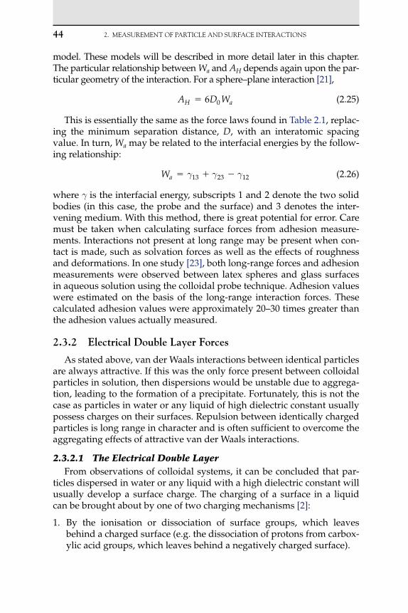
44 2. MEASUREMENTOFPARTICLEANdSURFACEINTERACTIONS
model. These models will be described in more detail later in this chapter. The particular relationship between Wa and AH depends again upon the par-ticular geometry of the interaction. For a sphere–plane interaction [21],
A D WH a 6 0 (2.25)
This is essentially the same as the force laws found in Table 2.1, replac-ing the minimum separation distance, D, with an interatomic spacing value. In turn, Wa may be related to the interfacial energies by the follow-ing relationship:
Wa 13 23 12 (2.26)
where is the interfacial energy, subscripts 1 and 2 denote the two solid bodies (in this case, the probe and the surface) and 3 denotes the inter-vening medium. With this method, there is great potential for error. Care must be taken when calculating surface forces from adhesion measure-ments. Interactions not present at long range may be present when con-tact is made, such as solvation forces as well as the effects of roughness and deformations. In one study [23], both long-range forces and adhesion measurements were observed between latex spheres and glass surfaces in aqueous solution using the colloidal probe technique. Adhesion values were estimated on the basis of the long-range interaction forces. These calculated adhesion values were approximately 20–30 times greater than the adhesion values actually measured.
2.3.2 Electrical double layer Forces
As stated above, van der Waals interactions between identical particles are always attractive. If this was the only force present between colloidal particles in solution, then dispersions would be unstable due to aggrega-tion, leading to the formation of a precipitate. Fortunately, this is not the case as particles in water or any liquid of high dielectric constant usually possess charges on their surfaces. Repulsion between identically charged particles is long range in character and is often sufficient to overcome the aggregating effects of attractive van der Waals interactions.
2.3.2.1 The Electrical Double LayerFrom observations of colloidal systems, it can be concluded that par-
ticles dispersed in water or any liquid with a high dielectric constant will usually develop a surface charge. The charging of a surface in a liquid can be brought about by one of two charging mechanisms [2]:
1. By the ionisation or dissociation of surface groups, which leaves behind a charged surface (e.g. the dissociation of protons from carbox-ylic acid groups, which leaves behind a negatively charged surface).

2.3 INTERACTIONFORCES 45
2. By the adsorption (binding) of ions from solution onto a previously uncharged surface. The adsorption of ions from solution can also occur onto oppositely charged sites, also known as ion exchange.
Since the system as a whole is electrically neutral, the dispersing medium must contain an equivalent charge of the opposite sign. These charges are carried by ions, i.e., by an excess of ions of one sign on the particle surface and an excess of ions of the opposite sign in the solution. Hence, if we consider an individual particle immersed in the liquid, it is surrounded by an electrical double layer. One part of this double layer is formed by the charge of the surface of the particles. Another part of the electrical double layer is formed by the excess of oppositely charged ions in the solution. As a result of their thermal motion, the electrical charge carried by this layer extends over a certain distance from the particle sur-face and dies out gradually with increasing distance (diffuse layer) into the bulk liquid phase.
2.3.2.2 Distribution of Electrical Charge and Potential in the Double Layer
The first approximate theory for the electrical double layer was given by Gouy, Chapman, Debye and Hückel [24]. In this theory, the average charge distribution and the corresponding electrical potential function have been related on the basis of the Poisson–Boltzmann equation (PBE) [18]:
∇2
0
01
ε ε
ri i
i
Bi
n z ez ek T
exp
∑
(2.27)
where is the electrical potential, ni0 is the number density of ions of
valency zi, kB is the Boltzmann constant, T is the absolute temperature, ε0 is the permittivity of vacuum, εr is the dielectric constant of the back-ground solvent and e is the elementary charge.
The above PBE has been deduced using a number of simplify-ing assumptions that the electrolyte is an ideal solution with uniform dielectric properties, the ions are point charges and the potential of mean force and the average electrostatic potential are identical. Besides, the PBE is only applicable to the system with a symmetrical electrolyte or a mixture of electrolytes of the same valency type. According to this theory, the average charge density at a given point can be calculated from the average value of the electrical potential at the same point with Boltzmann’s theorem. The electrical potential distribution can be related to the charge density with the aid of Poisson’s equation. As a matter of fact, the Gouy–Chapman theory has a rather serious defect, which is mainly a consequence of the neglect of the finite dimensions of the ions.

46 2. MEASUREMENTOFPARTICLEANdSURFACEINTERACTIONS
In dilute solutions, where the extension of the diffuse layer is consider-able, this neglect is to some degree permissible; but in more concentrated electrolyte solutions, the picture in terms of the Gouy–Chapman model becomes incorrect in some essential details.
Stern [25] modified the Gouy–Chapman model by taking into consid-eration the finite size of real ions, underlying the double layer theory for a solid wall by dividing the charges in liquid into two parts. One part is considered as a layer of ions adsorbed to the wall, and is represented in the theory by a surface charge concentrated in a plane at a small distance, d, from the surface charge on the wall, also known as the outer Helmholtz plane (OHP), as shown in Figure 2.4. The second part of the liquid charge is then taken to be a diffuse space charge, as in the old theory, extending from the OHP at x d to infinity, where the PBE can be applied.
The method with which the distance to the OHP is calculated depends on the type of model used for describing the compact region. For an oxide surface, such as typically found on the surface of silica, a triple layer model such as the Gouy–Chapman–Grahame–Stern model [26] is often used to describe the compact region; see Figure 2.4(a). This model allows for a plane of adsorbed ions (partially dehydrated) on the parti-cle surface (the centres of which form the locus for the inner Helmholtz plane (IHP)) followed by a plane occurring at the distance of closest approach of the hydrated counterions (the OHP). This is the mechanism by which the high surface charge on the oxide is reconciled with the quite low diffuse double layer potentials (zeta potentials). For other types of
IHP
σd
dψd
x = 0 iψ = ψo ψiσ = σo σi
εr2εr1
Particlesurface
Aqueoussolution
+
+
+–
–
–
–
–
–
+
OHP
εr1
OHP
σd
dψd
x = 0ψ = ψoσ = σo
Particlesurface
Aqueoussolution
–
–
–
–
–
–
+
+
+
A B
FIGuRE 2.4 Models for compact part of the double layer: (A) Gouy–Chapman–Grahame–Stern (triple layer) model and (B) modified Gouy–Chapman model.
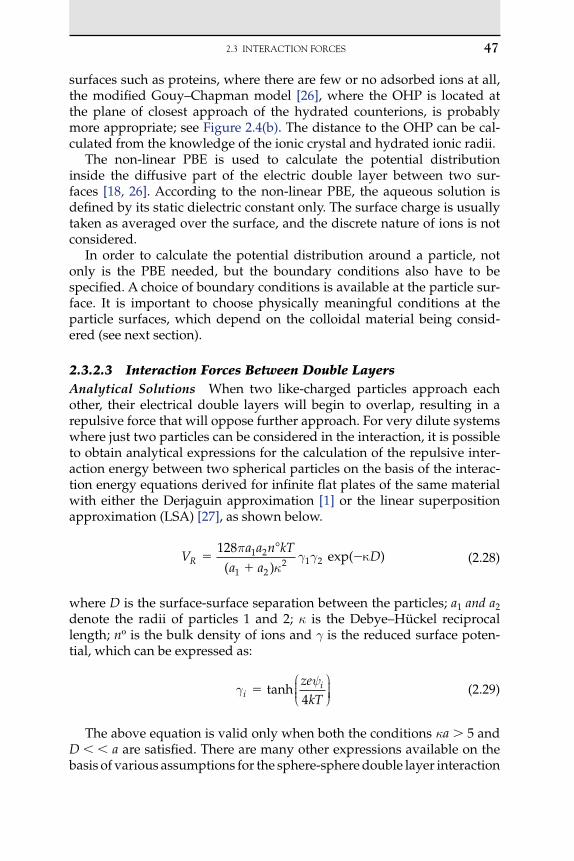
2.3 INTERACTIONFORCES 47
surfaces such as proteins, where there are few or no adsorbed ions at all, the modified Gouy–Chapman model [26], where the OHP is located at the plane of closest approach of the hydrated counterions, is probably more appropriate; see Figure 2.4(b). The distance to the OHP can be cal-culated from the knowledge of the ionic crystal and hydrated ionic radii.
The non-linear PBE is used to calculate the potential distribution inside the diffusive part of the electric double layer between two sur-faces [18, 26]. According to the non-linear PBE, the aqueous solution is defined by its static dielectric constant only. The surface charge is usually taken as averaged over the surface, and the discrete nature of ions is not considered.
In order to calculate the potential distribution around a particle, not only is the PBE needed, but the boundary conditions also have to be specified. A choice of boundary conditions is available at the particle sur-face. It is important to choose physically meaningful conditions at the particle surfaces, which depend on the colloidal material being consid-ered (see next section).
2.3.2.3 Interaction Forces Between Double LayersAnalytical Solutions When two like-charged particles approach each other, their electrical double layers will begin to overlap, resulting in a repulsive force that will oppose further approach. For very dilute systems where just two particles can be considered in the interaction, it is possible to obtain analytical expressions for the calculation of the repulsive inter-action energy between two spherical particles on the basis of the interac-tion energy equations derived for infinite flat plates of the same material with either the Derjaguin approximation [1] or the linear superposition approximation (LSA) [27], as shown below.
V
a a n kT
a aR
128 1 2
1 22 1 2
π
( ) exp( )κD
(2.28)
where D is the surface-surface separation between the particles; a1 and a2 denote the radii of particles 1 and 2; is the Debye–Hückel reciprocal length; no is the bulk density of ions and is the reduced surface poten-tial, which can be expressed as:
i
izekT
tanh4
(2.29)
The above equation is valid only when both the conditions a 5 and D a are satisfied. There are many other expressions available on the basis of various assumptions for the sphere-sphere double layer interaction
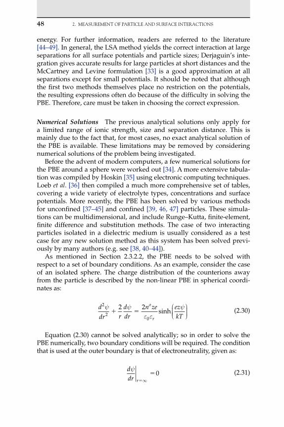
48 2. MEASUREMENTOFPARTICLEANdSURFACEINTERACTIONS
energy. For further information, readers are referred to the literature [44–49]. In general, the LSA method yields the correct interaction at large separations for all surface potentials and particle sizes; Derjaguin’s inte-gration gives accurate results for large particles at short distances and the McCartney and Levine formulation [33] is a good approximation at all separations except for small potentials. It should be noted that although the first two methods themselves place no restriction on the potentials, the resulting expressions often do because of the difficulty in solving the PBE. Therefore, care must be taken in choosing the correct expression.
Numerical Solutions The previous analytical solutions only apply for a limited range of ionic strength, size and separation distance. This is mainly due to the fact that, for most cases, no exact analytical solution of the PBE is available. These limitations may be removed by considering numerical solutions of the problem being investigated.
Before the advent of modern computers, a few numerical solutions for the PBE around a sphere were worked out [34]. A more extensive tabula-tion was compiled by Hoskin [35] using electronic computing techniques. Loeb et al. [36] then compiled a much more comprehensive set of tables, covering a wide variety of electrolyte types, concentrations and surface potentials. More recently, the PBE has been solved by various methods for unconfined [37–45] and confined [39, 46, 47] particles. These simula-tions can be multidimensional, and include Runge–Kutta, finite-element, finite difference and substitution methods. The case of two interacting particles isolated in a dielectric medium is usually considered as a test case for any new solution method as this system has been solved previ-ously by many authors (e.g. see [38, 40–44]).
As mentioned in Section 2.3.2.2, the PBE needs to be solved with respect to a set of boundary conditions. As an example, consider the case of an isolated sphere. The charge distribution of the counterions away from the particle is described by the non-linear PBE in spherical coordi-nates as:
ddr r
ddr
n ze ezkT
o
r
2
20
2 2 ε ε
sinh
(2.30)
Equation (2.30) cannot be solved analytically; so in order to solve the PBE numerically, two boundary conditions will be required. The condition that is used at the outer boundary is that of electroneutrality, given as:
ddr
r
∞
0
(2.31)
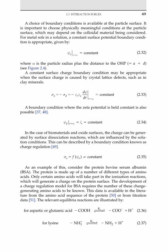
2.3 INTERACTIONFORCES 49
A choice of boundary conditions is available at the particle surface. It is important to choose physically meaningful conditions at the particle surface, which may depend on the colloidal material being considered. For metal sols in a solution, a constant surface potential boundary condi-tion is appropriate, given by:
o r
α
constant
(2.32)
where is the particle radius plus the distance to the OHP ( a d) (see Figure 2.4).
A constant surface charge boundary condition may be appropriate when the surface charge is caused by crystal lattice defects, such as in clay minerals.
ε ε
o d r o
r
ddr
α
constant
(2.33)
A boundary condition where the zeta potential is held constant is also possible [37, 48].
d r=α ζ constant (2.34)
In the case of biomaterials and oxide surfaces, the charge can be gener-ated by surface dissociation reactions, which are influenced by the solu-tion conditions. This can be described by a boundary condition known as charge regulation [49].
o o f ( ) constant≠ (2.35)
As an example of this, consider the protein bovine serum albumin (BSA). The protein is made up of a number of different types of amino acids. Only certain amino acids will take part in the ionisation reactions, which will generate a charge on the protein surface. The development of a charge regulation model for BSA requires the number of these charge-generating amino acids to be known. This data is available in the litera-ture from the amino acid sequence of the protein [50] or from titration data [51]. The relevant equilibria reactions are illustrated by:
for aspartic or glutamic acid COOH COO HK
1 (2.36)
for lysine NH NH HK
3 2
2 (2.37)
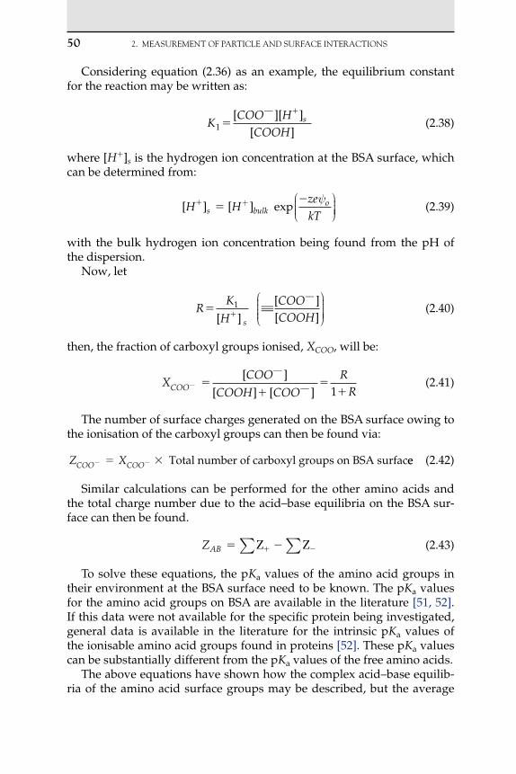
50 2. MEASUREMENTOFPARTICLEANdSURFACEINTERACTIONS
Considering equation (2.36) as an example, the equilibrium constant for the reaction may be written as:
K
COO H COOH
s1
[ ][ ][ ]
ˆ
(2.38)
where [H]s is the hydrogen ion concentration at the BSA surface, which can be determined from:
[ ] [ ] expH H
zekTs bulk
o +
(2.39)
with the bulk hydrogen ion concentration being found from the pH of the dispersion.
Now, let
R
K
H
COOCOOH s
1
[ ]
[ ][ ]
˜ˆ
(2.40)
then, the fraction of carboxyl groups ionised, XCOO, will be:
X
COOCOOH COO
R
RCOOˆ
ˆˆ
[ ][ ] [ ] 1
(2.41)
The number of surface charges generated on the BSA surface owing to the ionisation of the carboxyl groups can then be found via:
Z XCOO COOˆ ˆ Total number of carboxyl groups on BSA surfacee (2.42)
Similar calculations can be performed for the other amino acids and the total charge number due to the acid–base equilibria on the BSA sur-face can then be found.
ZAB ∑ ∑ (2.43)
To solve these equations, the pKa values of the amino acid groups in their environment at the BSA surface need to be known. The pKa values for the amino acid groups on BSA are available in the literature [51, 52]. If this data were not available for the specific protein being investigated, general data is available in the literature for the intrinsic pKa values of the ionisable amino acid groups found in proteins [52]. These pKa values can be substantially different from the pKa values of the free amino acids.
The above equations have shown how the complex acid–base equilib-ria of the amino acid surface groups may be described, but the average

2.3 INTERACTIONFORCES 51
net molecular charge of the BSA molecule will also depend on whether some surface groups on the molecule will also be involved with ionic equilibria with other ions in the electrolyte solution. For BSA, chloride binding will occur [53]. This chloride binding may be described by [54]:
Z Cl ze
kT
Cl zekT
Cl
o
o
440
1 44
[ ] exp
[ ] exp
ψ
ψ
( )( ))
( )(
Cl ze
kT
Cl zekT
o
o
33
1 1 1
γ ψ
γ ψ
[ ] exp
[ ] exp
. ))
(2.44)
where is the activity coefficient of the chloride ion at the particle sur-face (determined from activity coefficient data for NaCl solutions).
Therefore, the overall surface charge number of a BSA molecule is:
Z Z ZT AB Cl (2.45)
When solving the PBE using charge regulation as a boundary condi-tion, the compact part of the double layer around the BSA molecule needs to be taken into account. Figure 2.4(b) illustrates the model assumed for the compact part of the double layer. This model can be termed the Zeroth-order Stern model [55], as we have a zone of thickness, d, that is devoid of ions and represents a distance of closest approach to the par-ticle surface of charge density o. From electroneutrality,
o d (2.46)
From the solution of the PBE, d can be determined as:
ε ε
d o r
r a d
ddr
(2.47)
The surface potential of the particle, o, may also be determined by allowing for the capacitance of the fluid in the compact layer around the sphere. For two concentric spheres, the capacitance, C, may be deter-mined using [56]:
C
a ao r
4πε εαα
(2.48)
where a is the radius of the inner sphere and ( a d) is the radius of the outer sphere.
The capacitance can also be evaluated from the surface charge density as:
C
QV
a
o
o d
∆π4 2
(2.49)

52 2. MEASUREMENTOFPARTICLEANdSURFACEINTERACTIONS
Combining equations (2.48) and (2.49),
ε εo
o
o rd
ada d
( ) (2.50)
The surface potential can therefore be established if a, d, d, o, εo and εr are known. The value for the dielectric constant for the compact layer, εr, is unknown, but for the model used here, it has been shown that the bulk dielectric constant for water may be used if d is in the range 0.1–0.3 nm [55]. Thus, from an initial guess for d, d (and thus o) may be deter-mined from the solution of the non-linear PBE (which gives d dr r a d/ ). From these values, the surface potential, o, can be evaluated from equa-tion (2.50) and then the number of charges on the BSA molecule may be determined from the charge regulation model. Using ZT, a value for the surface charge density may be recalculated.
πoT
Z e
a
4 2
(2.51)
The two values for the surface charge calculated, via the PBE and the surface charge model, may then be compared for a given d and an itera-tion may be performed on d until the surface charge calculated via both methods is equivalent. In this way, for given dispersion conditions (pH, ionic strength, concentration), the value of the potential at the OHP may be determined. This potential is widely considered to be the zeta poten-tial of the molecule [57]. The calculated value of the zeta potential may be compared to the value obtained experimentally from electrophoresis measurements on dilute BSA dispersions [58].
Once the PBE has been solved, calculation of the interaction energy may be performed using an appropriate model.
In the case of concentrated colloidal dispersions, however, the interac-tion energy between particles (as in a gel layer) is multiparticle in nature, so modification of the two-body interaction has to be made in order to allow for multiparticle interactions. A method by which the multiparti-cle nature of such interactions can be taken into account is to use a cell model [59] combined with a numerical solution of the non-linear PBE in spherical coordinates [60–64]. This cell model is based on the Wigner and Seitz cell model [65] that approximated the free electron energy of a crystal lattice by calculating the energy of a single crystal, since it has the same symmetry as the lattice.
The concentrated colloidal dispersion can now be considered as being divided into spherical cells so that each cell contains a single particle and a concentric spherical shell of an electrolyte solution, having an outer radius of certain magnitude such that the particle cell volume ratio in the unit cell is equal to the particle volume fraction throughout the entire
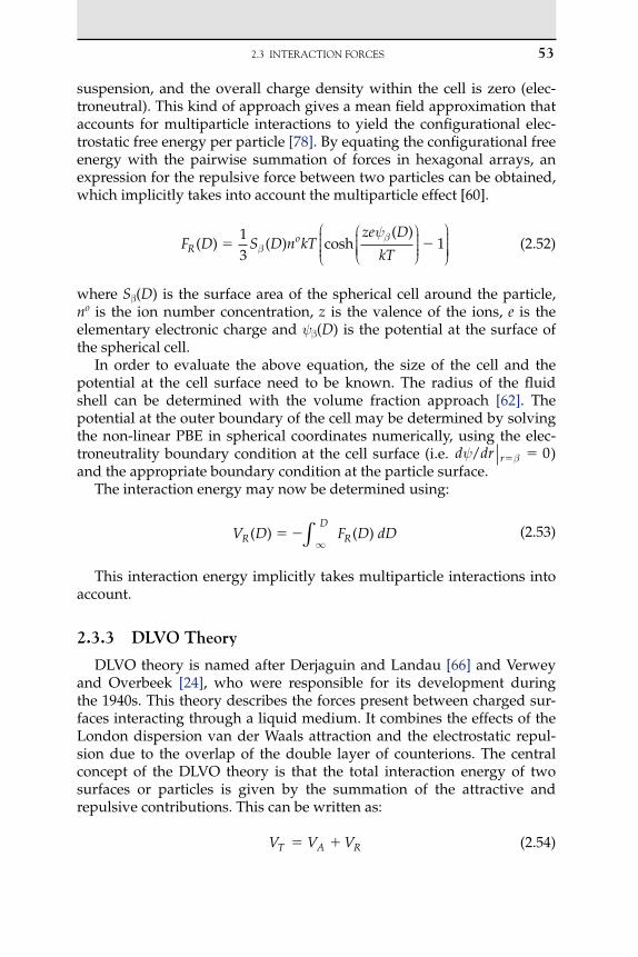
2.3 INTERACTIONFORCES 53
suspension, and the overall charge density within the cell is zero (elec-troneutral). This kind of approach gives a mean field approximation that accounts for multiparticle interactions to yield the configurational elec-trostatic free energy per particle [78]. By equating the configurational free energy with the pairwise summation of forces in hexagonal arrays, an expression for the repulsive force between two particles can be obtained, which implicitly takes into account the multiparticle effect [60].
F D S D n kT
ze D
kTRo( ) ( ) cosh
( )
13
1ββ
(2.52)
where S(D) is the surface area of the spherical cell around the particle, no is the ion number concentration, z is the valence of the ions, e is the elementary electronic charge and (D) is the potential at the surface of the spherical cell.
In order to evaluate the above equation, the size of the cell and the potential at the cell surface need to be known. The radius of the fluid shell can be determined with the volume fraction approach [62]. The potential at the outer boundary of the cell may be determined by solving the non-linear PBE in spherical coordinates numerically, using the elec-troneutrality boundary condition at the cell surface (i.e. d dr r β/ 0) and the appropriate boundary condition at the particle surface.
The interaction energy may now be determined using:
V D F D dDR
D
R( ) ( )
∞∫ (2.53)
This interaction energy implicitly takes multiparticle interactions into account.
2.3.3 dlVo theory
DLVO theory is named after Derjaguin and Landau [66] and Verwey and Overbeek [24], who were responsible for its development during the 1940s. This theory describes the forces present between charged sur-faces interacting through a liquid medium. It combines the effects of the London dispersion van der Waals attraction and the electrostatic repul-sion due to the overlap of the double layer of counterions. The central concept of the DLVO theory is that the total interaction energy of two surfaces or particles is given by the summation of the attractive and repulsive contributions. This can be written as:
V V VT A R (2.54)

54 2. MEASUREMENTOFPARTICLEANdSURFACEINTERACTIONS
where the total interaction energy VT is expressed in terms of the repul-sive double layer interaction energy VR and the attractive London–van der Waals energy VA. For a measurement made between a spherical col-loid probe and a plain surface, this can be adapted to give the relation-ship for a normalised force:
FR
V VA R 2π( )
(2.55)
Contrary to the double layer interaction, the van der Waals interaction energy is mostly insensitive to variations in electrolyte strength and pH. Additionally, the van der Waals attraction must always be greater than the double layer repulsion at extremely small distances since the inter-action energy satisfies a power law (i.e. VA Dn), whereas the dou-ble layer interaction energy remains finite or increases far more slowly within the same small separation range.
DLVO theory was challenged by the existence of long-range attractive electrostatic forces between particles of like charge. The established the-ory of colloidal interactions predicts that an isolated pair of like-charged colloidal spheres in an electrolyte should experience a purely repulsive screened electrostatic (Coulombic) interaction. The experimental evi-dence, however, indicates that the effective interparticle potential can have a long-range attractive component in more concentrated suspen-sions [67, 68] and for particles confined by charged glass walls [69, 70]. The explanations for the observation are divided and debatable. One of the arguments [71] demonstrated that the attractive interaction measured between like-charged colloidal spheres near a wall can be accounted for by a non-equilibrium hydrodynamic effect, which was proved by both analytical results and Brownian dynamics simulations.
2.3.3.1 Measurement of DLVO Forces Using Atomic Force MicroscopyThe following section will review a number of papers describing
experiments to measure van der Waals and electrostatic double layer forces between particles using the colloidal probe technique, but should not be considered as a complete coverage of published information. For further reading, there are a number of excellent reviews that may be rec-ommended [13, 21, 72–74].
The first use of AFM to measure interactions between a colloidal par-ticle and a surface was reported by Ducker and colleagues, where a sil-ica sphere was allowed to interact with a silica surface in aqueous NaCl solutions [4, 75]. Force measurements were fitted with theoretical force laws for DLVO theory, combining van der Waals and electrostatic double layer interactions. For separations greater than 3 nm, observations agreed favourably with the conventional DLVO theory. However, at closer
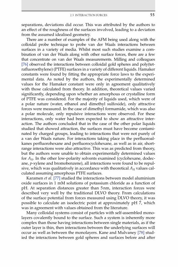
2.3 INTERACTIONFORCES 55
separations, deviations did occur. This was attributed by the authors to an effect of the roughness of the surfaces involved, leading to a deviation from the assumed idealised geometry.
There are a number of examples of the AFM being used along with the colloidal probe technique to probe van der Waals interactions between surfaces in a variety of media. Whilst most such studies examine a com-bination of van der Waals along with other surface forces, there are a few that concentrate on van der Waals measurements. Milling and colleagues [76] observed the interactions between colloidal gold spheres and poly(tet-rafluoroethylene) (PTFE) surfaces in a variety of different liquids. Hamaker constants were found by fitting the appropriate force laws to the experi-mental data. As noted by the authors, the experimentally determined values for the Hamaker constant were only in agreement qualitatively with those calculated from theory. In addition, theoretical values varied significantly, depending upon whether an amorphous or crystalline form of PTFE was considered. For the majority of liquids used, which were of a polar nature (water, ethanol and dimethyl sulfoxide), only attractive forces were measured. In the case of dimethyl formamide, which was also a polar molecule, only repulsive interactions were observed. For these interactions, only water had been expected to show an attractive inter-action. The authors concluded that in the case of the other polar liquids studied that showed attraction, the surfaces must have become contami-nated by charged groups, leading to interactions that were not purely of a van der Waals nature. For interactions taking place in the perfluoroal-kanes perfluorohexane and perfluorocyclohexane, as well as in air, short-range interactions were also attractive. This was as predicted from theory, but the authors were unable to obtain experimentally determined values for AH. In the other low-polarity solvents examined (cyclohexane, dodec-ane, p-xylene and bromobenzene), all interactions were found to be repul-sive, which was qualitatively in accordance with theoretical AH values cal-culated assuming amorphous PTFE surfaces.
Karamen et al. [77] studied the interactions between model aluminium oxide surfaces in 1 mM solutions of potassium chloride as a function of pH. At separation distances greater than 5 nm, interaction forces were described very well by the traditional DLVO theory. From calculations of the surface potential from forces measured using DLVO theory, it was possible to calculate an isoelectric point at approximately pH 7, which was in agreement with values obtained from the literature.
Many colloidal systems consist of particles with self-assembled mono-layers covalently bound to the surface. Such a system is inherently more complex than those having interactions between single materials, as if the outer layer is thin, then interactions between the underlying surfaces will occur as well as between the monolayers. Kane and Mulvaney [78] stud-ied the interactions between gold spheres and surfaces before and after

56 2. MEASUREMENTOFPARTICLEANdSURFACEINTERACTIONS
the deposition of mercaptoundecanoic acid (MUA). Force measurements at different electrolyte concentrations and pH values were fitted with a modified DLVO theory to determine surface potentials and Hamaker constants. The adsorption of the MUA itself was found to substantially decrease the magnitude of the dispersive forces between the gold sur-faces. It was also found that the degree of ionisation of the surface car-boxy groups was very low. The authors applied two models to explain these results. It was concluded that either a thicker-than-usually-expected Stern layer was present or that strong competitive binding of cations was the cause. Surface interactions between particles and surfaces with more complex attached monolayers, such as proteins, have also been investi-gated. Bowen et al. [79] investigated systems of silica microspheres and surfaces co-incubated to give an adsorbed layer of bovine serum albu-min (BSA) at different values of pH and NaCl concentrations. Figure 2.5 shows a plot of representative force curves obtained as a BSA-coated silica sphere approached a BSA-coated silica surface in aqueous NaCl solutions of differing ionic strengths. As the ionic strength was increased, both the range and magnitude of repulsive interactions increased. For the three highest NaCl concentrations, experimental observations were in good agreement with the values predicted from DLVO theory and zeta potential values. The zeta potentials for the BSA were calculated using a site-dissociation-site-binding approach from the amino acid sequence [58, 80]. At the lowest ionic strength examined (0.0002 M NaCl), the observed values were higher than those predicted from theory.
Distance [nm]0 5 10 15 20 25 30
0.0001
0.01
0.1
1
Nor
mal
ised
forc
e, F
/R (m
N/m
)
FIGuRE 2.5 Plot of normalised force versus separation distance plot for silica surfaces coated with monolayers of BSA at four concentrations of NaCl at pH 8.0: () 0.1 M; () 0.01 M; () 0.001 M; () 0.0002 M. The lines are theoretical predictions from DLVO theory.

2.3 INTERACTIONFORCES 57
Interaction between colloidal particles and filtration media is of much interest industrially, due to the propensity of dispersed particles to foul membrane surfaces and reduce their efficiency [81, 82]. As under condi-tions in which membrane filtration most often occurs both the mem-brane and dispersed colloids and other particles carry surface charges, the strength and sign of electrical double layer interactions are of great importance. The forces involved in the approach of a colloidal particle to a membrane surface are essentially a balance between electrical double layer interactions and hydrodynamic forces. Studies have been made of double layer interactions using model silica colloidal spheres and poly-meric microfiltration membranes [83]. Solutions of NaCl were prepared of varying ionic strengths at a single pH value (pH 8.0). Representative force curves for each approach made by the silica probe to membrane sur-faces are shown in Figure 2.6. At all ionic strengths, forces were signifi-cantly repulsive at all separation distances, showing that the electrostatic double layer repulsion is dominant in all cases. The range that the repul-sive interactions first become detectable increased from approximately 10 nm at 101 M NaCl to approximately 35 nm at 104 M. When mea-surements were made in high purity water, this increased to 60 nm. The change in the magnitude of the forces with decreasing ionic strength is in accordance with electrical double layer theory, with the decay lengths of the measured force curves comparable to the Debye charge screening lengths of the different ionic strength solutions under study. The decrease
Distance [nm]0 5 10 15 20 25 30 35 40 45
F/R
[mN
/m]
0
5
10
15
20
10�4 M NaCl10�3 M NaCl10�2 M NaCl10�1 M NaCl
FIGuRE 2.6 Plot showing normalised force versus separation distance for the approach of a silica colloid probe towards a microfiltration membrane surface at different salt concen-trations. As the concentration of NaCl is increased, repulsive forces on approach decrease owing to charge screening effects.

58 2. MEASUREMENTOFPARTICLEANdSURFACEINTERACTIONS
in repulsive interaction between the particles and the membrane with the increase in the salt concentration has implications for membrane filtration processes, but especially for the desalination treatment of water. Brant and Childress [84] studied the long-range interaction forces between colloids of a variety of materials (silica, alumina and polystyrene) with reverse osmosis membranes and developed an extended DLVO theory that added the effect of acid–base interactions, with AFM experiments used to vali-date the extended theory. It was found that for interactions between two hydrophilic surfaces, the extended theory fitted the data better than clas-sical theory, demonstrating the importance of acid–base interactions for this configuration. For interactions between hydrophobic materials, the extended theory was not significantly different from the classical theory, as would be expected for interactions between non-polar materials.
2.3.4 Solvation Forces
The DLVO theory successfully explains the long-range interaction forces observed in a large number of systems (colloids, surfactant solu-tions, lipid bilayers etc.) in terms of the electrical double layer and London–van der Waals forces. However, when two surfaces or particles approach closer than a few nanometres, the interactions between two solid surfaces in a liquid medium fail to be accounted for by DLVO theory. This is because the theories of van der Waals and double layer forces discussed in the previous sections are both continuum theories, described on the basis of the bulk properties of the intervening solvent such as its refrac-tive index, dielectric constant and density, whereas the individual nature of the molecules involved, such as their discrete size, shape and chemis-try, was not taken into consideration by DLVO theory. Another explana-tion for this is that other non-DLVO forces come into play, although the physical origin of such forces is still somewhat obscure [85, 86]. These additional forces can be monotonically repulsive, monotonically attractive or even oscillatory in some cases. And these forces can be much stronger than either of the two DLVO forces at small separations [2, 87].
To understand how the additional forces arise between two surfaces a few nanometers apart, we need to start with the simplest but most gen-eral case of inert spherical molecules between two smooth surfaces, first considering the way solvent molecules order themselves at a solid–liquid interface, then considering how this structure corresponds to the presence of a neighbouring surface and how this in turn brings about the short-range interaction between two surfaces in the liquid. Usually, the liquid structure close to an interface is different from that in the bulk. For many liquids, the density profile normal to a solid surface oscillates around the bulk density, with a periodicity of a molecular diameter in a nar-row region near the interface. This region typically extends over several

2.3 INTERACTIONFORCES 59
molecular diameters. Within this range, the molecules are ordered in lay-ers according to some theoretical work and particularly computer simu-lations [88, 89] as well as experimental observations [90, 91]. When two such surfaces approach each other, one layer of molecules after another is squeezed out of the closing gap. The geometric constraining effect of the approaching wall on these molecules and attractive interactions between the surface and liquid molecules hence create the solvation force between the two surfaces. For simple spherical molecules between two hard, smooth surfaces, the solvation force is usually a decaying oscillatory function of distance. For molecules with asymmetric shapes or whose interaction potentials are anisotropic or not pairwise additive, the result-ing solvation force may also have a monotonically repulsive or attractive component. When the solvent is water, they are referred to as hydration forces. Solvation forces depend both on the chemical and physical prop-erties of the surfaces being considered, such as the wettability, crystal structure, surface morphology and rigidity and on the properties of the intervening medium.
The hydration force is one of the most widely studied and controver-sial non-DLVO forces, a strong short-range force that decays exponen-tially with the distance, D, between the surfaces [92, 93]:
F D KeSOLD l( ) /
(2.56)
where K 0 relates to the hydrophilic repulsion forces, K 0 relates to the hydrophobic attraction forces and l is the correlation length of the ori-entational ordering of water molecules.
The concept of the hydration force emerged to explain measurements of forces between neutral lipid bilayer membranes [93]. Its presence in charged systems is controversial, but there is experimental evidence of non-DLVO forces following equation (2.56) in systems as diverse as dihexadecyldimethyl ammonium acetate surfactant bilayers [94], DNA polyelectrolyte solutions [95] and charged polysaccharides [96]. In these experiments, the hydration forces show little sensitivity to ionic strength.
Many theoretical studies and computer simulations of various con-fined liquids, including water, have invariably led to a solvation force described by an exponentially decaying cos-function of the form [97–100]:
F D f
DeSOL
m
D D( ) 0
20cos /π
(2.57)
where FSOL is the force per unit area; f0 is the force extrapolated to separation distance, D 0; m is the molecular diameter and D0 is the characteristic decay length.

60 2. MEASUREMENTOFPARTICLEANdSURFACEINTERACTIONS
A repulsive force dominant at short ranges between silica surfaces in aqueous solutions of NaCl has been reported by Grabbe and Horn [101], which was also found to be independent of electrolyte concentration over the range investigated. They attributed this force to a hydration repulsion resulting from hydrogen bonding of water to the silica surface, and fitted the additional component to a sum of two exponentials to work out the formula for the hydration forces in the system.
The physical mechanisms underlying the hydration force are still a matter for debate. One possible mechanism is the anomalous polarisa-tion of water near the interfaces, which completely alters its dielectric response [102–104]. These theories imply an electrostatic origin of the hydration force. However, other authors report [105] that there is no evidence for a significant structuring of water layers near interfaces, or a perturbation of its dielectric response, as envisaged by previous theo-ries. Instead, they suggest that the repulsive forces are due to entropic (osmotic) repulsion of thermally excited molecular groups that protrude from the surfaces [106]. This theory explains many experimental obser-vations in neutral systems [107], but its validity in charged systems is not certain. Given the available evidence from experiments and simulations, it is not possible to reach a definitive conclusion on the precise role of these mechanisms in determining the hydration forces. Until recently, computer simulations of water films coated with ionic surfactants showed that protrusions are not significant in these systems [108]. On the other hand, computer simulations show that water has an anomalous dielectric behaviour near charged interfaces [109], but the observed elec-trostatic fields obviously differ from the predictions of electrostatic theo-ries on hydration forces [103, 110]. The effect of this anomalous dielectric behaviour of water on the electrostatic force between surfaces or inter-faces is still unknown.
The use of AFM to measure solvation forces between surfaces has been of some interest amongst researchers in recent years for the purposes of both studying the phenomena between closely interacting probes and surfaces that may cause artefacts when imaging with an AFM and inves-tigating the effect of these solvation forces on the interactions between colloidal particles. O’Shea and colleagues [111] observed an oscillatory force on close approach of a sharp AFM probe to a graphite surface in water, octamethylcyclotetra siloxane (OMCTS), and dodecanol. A series of repulsive barriers were observed as approach was made for OMCTS and dodecanol, with each repulsive barrier becoming successively larger, owing to the closer-bound solvation layers becoming harder to displace. The authors calculated that the energy required to remove the solva-tion molecules was 5–25 times kT for OMCTS and 5–1000 times kT for dodecanol, suggesting that only a small number of molecules were being displaced. In addition, it was noted that the distance between successive

2.3 INTERACTIONFORCES 61
oscillatory peaks compared well with the sizes of the molecules of inter-est, suggesting that each solvation shell consisted of a single layer of molecules. A later set of measurements in OMCTS and dodecanol on HOPG reached a similar conclusion [112, 113]. No displacement of solva-tion layers could be observed in water owing to the relatively large range and magnitude of the attractive jump-in event observed. In a later set of experiments [114], an oscillating lever was used to probe the solvation forces in OMCTS and dodecanol, allowing the mechanical compliance of the solvation shells to be measured. Here, periodic changes in the ampli-tude of lever oscillations were observed, which was explained as being because of an increase in the effective viscosity of the solutions when the surfaces were in close approach. It was noted that the presence of oscilla-tory structural forces even at the highly curved geometries present, even when using a sharp AFM probe, could have a detrimental influence on the very high resolution imaging of surfaces when using AFM.
Solvation forces were measured in primary alcohols between silicon nitride probes and mica and HOPG surfaces by Franz and Butt [115]. For the measurements made against the hydrophilic mica, no solvation oscil-lation forces were observed at separation distances of less than 4 nm. At distances less than this, repulsive maxima followed by sudden jump-in events were observed. These repeated maxima were ascribed to the pres-ence of solvation shells, with at least two of these layers present. These solvation forces were determined to be greater in magnitude than the attractive van der Waals forces present. It was noted that the period of the force oscillations increased linearly with chain length, with the period greater than the chain length. It was concluded that for the measure-ments made on mica, the molecules did not take on a flat conformation, but were at least partially upright. On the hydrophobic HOPG surface, measurements in 1-propanol and 1-pentanol oscillations had a period of 0.45 nm, suggesting that on the hydrophobic surface they did lie flat against the surface.
Valle-Delgado and colleagues [116] investigated the solvation forces in water between hydrophilic silica spheres versus plane silica surfaces. A repulsive force was measured (2 nm) at ranges shorter than the observed double layer repulsion and attractive van der Waals forces. A number of theoretical models were applied to the experimental data and it was concluded that for the situation under investigation, the obser-vations were best explained by the formation and rupture of hydrogen bonds between SiOH groups on the silica surfaces and a single layer of water molecules.
Jarvis et al. [117] used a carbon nanotube to probe solvation forces in water against a self-assembled monolayer bound to a gold surface, which had been characterised by imaging using the nanotube probe. When the forces were normalised, they were found to be in reasonable agreement

62 2. MEASUREMENTOFPARTICLEANdSURFACEINTERACTIONS
with previous measurements undertaken with the surface force appara-tus [118]. The authors concluded that the forces scaled along with the sur-face interaction dimensions between the mesoscale and nanoscale [117].
2.3.5 Steric Interaction Forces
For molecules attached to a solid surface in a liquid environment, chains with a degree of freedom to move will tend to dangle out into the solution where they remain thermally mobile. On approach of two poly-mer-covered surfaces, the entropy of confining these dangling chains results in a repulsive entropic force, which, for overlapping polymer molecules, is known as the steric or overlap repulsion. In ancient Egypt, people already knew how to keep ink stabilised by dispersing soot par-ticles in water, incubated with gum arabicum or egg-adsorbed polymers, which, in the first case, is a mixture of polysaccharide and glycoprotein and in the second mainly the protein albumin, which works through this steric repulsion. However, steric repulsion does not necessarily have to be due to polymeric molecules; layers of small molecules can have the same effect, albeit at a much shorter range.
Steric stabilisation of dispersions is very important in many industrial processes. This is because colloidal particles that normally coagulate in a solvent can often be stabilised by adding a small amount of polymer to the dispersing medium. Such polymer additives are known as protec-tives against coagulation and they lead to the steric stabilisation of a col-loid. Both synthetic polymers and biopolymers (e.g. protein, gelatine) are widely used in both non-polar and polar solvents (e.g. in paints, toners, emulsions, cosmetics, pharmaceuticals, processed food, soils, lubricants).
Theories of steric interactions are not well developed. There is no sim-ple, comprehensive theory available as steric forces are complicated and difficult to describe [119–121]. The magnitude of the force between surfaces coated with polymers depends on the quantity or coverage of polymer on each surface, on whether the polymer is simply adsorbed from solution (a reversible process) or irreversibly grafted onto the surfaces and finally on the quality of the solvent [119, 122]. Different components contribute to the force, and which component dominates the total force is situation specific.
For interactions in poor and theta solvents, there are some theories available for low and high surface coverage. In the case of the low cover-age where there is no overlap or entanglement of neighbouring chains, the repulsive energy per unit area is a complex series and roughly expo-nential [123–126]. As for the high coverage of end-grafted chains, the thickness of the brush layer increases linearly with the length of the poly-mer molecule. Once two brush-bearing surfaces are close enough to each other, there is a repulsive pressure between them, and this force can be approximated by the Alexander–de Gennes theory [119, 127, 128].
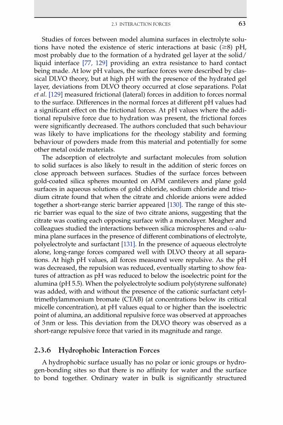
2.3 INTERACTIONFORCES 63
Studies of forces between model alumina surfaces in electrolyte solu-tions have noted the existence of steric interactions at basic (8) pH, most probably due to the formation of a hydrated gel layer at the solid/liquid interface [77, 129] providing an extra resistance to hard contact being made. At low pH values, the surface forces were described by clas-sical DLVO theory, but at high pH with the presence of the hydrated gel layer, deviations from DLVO theory occurred at close separations. Polat et al. [129] measured frictional (lateral) forces in addition to forces normal to the surface. Differences in the normal forces at different pH values had a significant effect on the frictional forces. At pH values where the addi-tional repulsive force due to hydration was present, the frictional forces were significantly decreased. The authors concluded that such behaviour was likely to have implications for the rheology stability and forming behaviour of powders made from this material and potentially for some other metal oxide materials.
The adsorption of electrolyte and surfactant molecules from solution to solid surfaces is also likely to result in the addition of steric forces on close approach between surfaces. Studies of the surface forces between gold-coated silica spheres mounted on AFM cantilevers and plane gold surfaces in aqueous solutions of gold chloride, sodium chloride and triso-dium citrate found that when the citrate and chloride anions were added together a short-range steric barrier appeared [130]. The range of this ste-ric barrier was equal to the size of two citrate anions, suggesting that the citrate was coating each opposing surface with a monolayer. Meagher and colleagues studied the interactions between silica microspheres and -alu-mina plane surfaces in the presence of different combinations of electrolyte, polyelectrolyte and surfactant [131]. In the presence of aqueous electrolyte alone, long-range forces compared well with DLVO theory at all separa-tions. At high pH values, all forces measured were repulsive. As the pH was decreased, the repulsion was reduced, eventually starting to show fea-tures of attraction as pH was reduced to below the isoelectric point for the alumina (pH 5.5). When the polyelectrolyte sodium poly(styrene sulfonate) was added, with and without the presence of the cationic surfactant cetyl-trimethylammonium bromate (CTAB) (at concentrations below its critical micelle concentration), at pH values equal to or higher than the isoelectric point of alumina, an additional repulsive force was observed at approaches of 3 nm or less. This deviation from the DLVO theory was observed as a short-range repulsive force that varied in its magnitude and range.
2.3.6 Hydrophobic Interaction Forces
A hydrophobic surface usually has no polar or ionic groups or hydro-gen-bonding sites so that there is no affinity for water and the surface to bond together. Ordinary water in bulk is significantly structured

64 2. MEASUREMENTOFPARTICLEANdSURFACEINTERACTIONS
because of hydrogen bonding between the water molecules. The coop-erative nature of this bonding [132] means that quite large clusters of hydrogen-bonded water molecules can form although they may contin-ually form and break down in response to thermal energy fluctuations. The orientation of water molecules in contact with a hydrophobic mol-ecule is entropically unfavourable; therefore, two such molecules tend to come together simply by attracting each other. As a result, the entro-pically unfavoured water molecules are expelled into the bulk and the total free energy of the system is reduced accordingly. The presence of a hydrophobic surface could restrict the natural structuring tendency of water by imposing a barrier that prevents the growth of clusters in a given direction. Similar effects occur between two hydrophobic surfaces in water. Water molecules confined in a gap between two such surfaces would thus be unable to form clusters larger than a certain size. For an extremely narrow gap, this could be a serious limitation and result in an increased free energy of the water in comparison with that in bulk. In other words, this would give rise to an attractive force between hydro-phobic surfaces as a consequence of water molecules migrating from the gap to the bulk water where there are unrestricted hydrogen-bonding opportunities and a lower free energy.
Attraction between hydrophobic surfaces has been measured directly [133] and can be of surprisingly long range, up to about 80 nm [134]. The attraction was much stronger than the van der Waals force and of much greater range. The interaction of filaments of hydrophobised silica was measured by Rabinovich and Derjaguin [135]. They found an attrac-tive force at large separation distances, one to two orders of magnitude greater than van der Waals attraction. There have been many experimen-tal measurements of the interaction force between various hydrophobic surfaces in aqueous solutions. These studies have found that the hydro-phobic force between two macroscopic surfaces is of extraordinarily long range, decaying exponentially with a characteristic decay length of 1–2 nm in the range 0–10 nm, and then more gradually further out, and this force can be much stronger than those predicted on the basis of van der Waals interaction, especially between hydrocarbon surfaces for which the Hamaker constant is quite small.
It is now well established that a long-range (10 nm) attractive force operates between hydrophobic surfaces immersed in water and aqueous solutions [136]. Unfortunately, so far, no generally accepted theory has been developed for these forces, but the hydrophobic force is thought to arise from overlapping solvation zones as two hydrophobic species come together [2]. In fact, Eriksson et al. [137] have used a square-gradient vari-ational approach to show that the mean field theory of repulsive hydra-tion forces can be modified to account for some aspects of hydrophobic attraction. Conversely, Ruckenstein and Churaev suggest a completely

2.3 INTERACTIONFORCES 65
different origin that attributes the attraction to the coalescence of vacuum gaps at the hydrophobic surfaces [138].
In recent years, a number of studies have been undertaken to study the effect of nanoscale bubbles found on hydrophobic surfaces to explain the hydrophobic forces reported in many surface force mea-surements. These bubbles may be present on the hydrophobic surfaces when first immersed in aqueous solutions, or may form from dissolved gases after immersion. Considine et al. [139], when undertaking mea-surements between two latex spheres, noted a large attractive force with a range much in excess of that expected from van der Waals attraction and independent of electrolyte concentration. They observed that degas-sing of solutions reduced the range of this attractive force significantly. Re-gassing of the solution restored the original range of this force, show-ing the influence of dissolved gas on the measurement of hydrophobic forces. Mahnke and colleagues [140] studied both the effect of dissolved gas and the degree of hydrophobicity of surfaces on the range of attrac-tive forces. When surfaces were used that gave large (25 nm) jump-in events, degassing of the intervening medium reduced the range of mea-surable attractive forces. For combinations of surfaces that gave short jump-in events, degassing of the solutions had little effect. It can be con-cluded that the long-range hydrophobic attraction can be accounted for by the presence of nanobubbles attached to the hydrophobic surfaces. The presence of such bubbles has been confirmed by the use of tapping mode AFM on hydrophobised silicon wafers [141, 142]. Bubble-like fea-tures observed on these surfaces show a high phase contrast with the rest of the surface, suggesting very different mechanical properties to the silicon surface. Force curves taken at the sites of these putative nano-bubbles show much greater attractive and adhesive forces with a hydro-phobic AFM probe than when taken from a bare area of the surface. Zhang and colleagues examined the effects of degassing and liquid tem-perature on the number and density on the surface of the nanobubbles [143]. Degassing of water and ethanol under vacuum reduced the sur-face density of nanobubbles to a very significant extent. Increasing the temperature of the fluid also increased the number and size of the nano-bubbles on the surface, a phenomena witnessed by another group who also observed the spontaneous appearance of nanobubbles as the liquid temperature was increased [144]. For measurements where the hydro-phobic force being measured is a result of the interaction of bubbles on the opposing surfaces, the forces measured are actually capillary forces rather than true hydrophobic forces, albeit capillary forces present as a result of the hydrophobicity of the surfaces. For those who wish to read further into the origins of forces measured between hydrophobic surfaces in aqueous solutions, the authors would like to draw attention to a num-ber of reviews in the literature [145–147].

66 2. MEASUREMENTOFPARTICLEANdSURFACEINTERACTIONS
2.3.7 Effect of Hydrodynamic drag on AFM Force Measurements
When performing measurements with particles in liquid, the effects of hydrodynamic drag on both the particle and also the cantilever may be sig-nificant, depending on the velocities at which measurements are taken. In particular, the effects of confinement of the liquid between two particles or between two surfaces are important. As the distance between the two sur-faces decreases, the finite drainage time for the confined liquid produces a force dependent on the separation distance, the velocity of the approach as well as the viscosity and density of the fluid medium. Ignoring any contri-bution of drag on the cantilever to this effect, the hydrodynamic force, FH, for a sphere approaching a plane surface is given by a modified version of Stoke’s law for the drag force on a sphere [148, 149]:
F rH c 6πν s (2.58)
where υ is the velocity of the probe, is the dynamic viscosity of the surrounding fluid, rs is the radius of the spherical particle and c is a cor-rection applied to Stoke’s law to account for the presence of the confining wall in close proximity.
c cn
c
n nn n
n n
43
12 1 2 3
2 2 1 2 1
1
sinh( )
( )( )
sinh( ) ( )
∞
∑
+ + sinh22
4 0 5 2 1 212 2
c
c cn nsinh ( ) ( ) sinh .−
(2.59)
where
cs
s
s
s
s
s
D rr
D rr
D rr
cosh ln1
2
1
(2.60)
where D is the distance between the plane surface and closest point of the sphere. For measurements where r h, then this can be simplified to:
F
rDH
s6 2πν
(2.61)
In most cases, contributions due to interactions between the surface and the cantilever itself can be neglected. However, depending on the size of the colloid probe and the speed at which the experiment is carried out, this may not always be the case. Vinogradova et al. [150] studied the
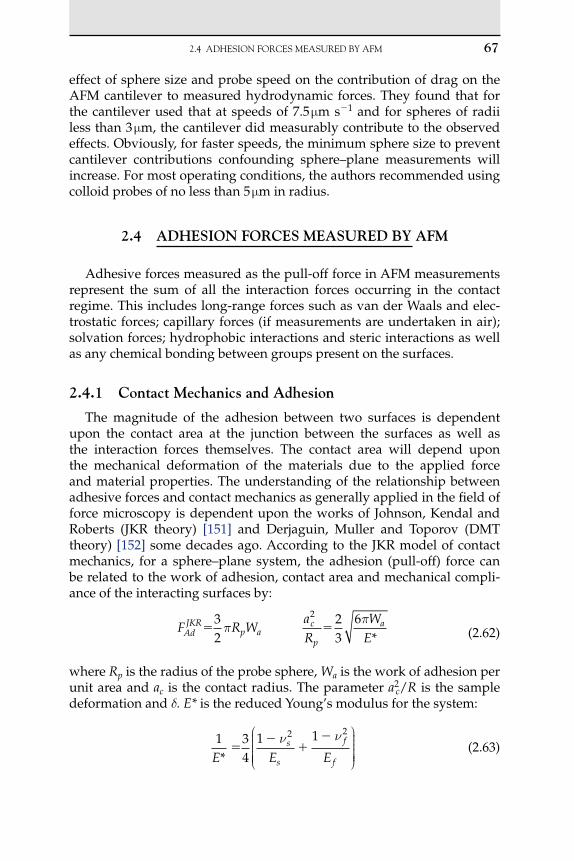
2.4 AdHESIONFORCESMEASUREdByAFM 67
effect of sphere size and probe speed on the contribution of drag on the AFM cantilever to measured hydrodynamic forces. They found that forthe cantilever used that at speeds of 7.5 m s1 and for spheres of radii less than 3 m, the cantilever did measurably contribute to the observed effects. Obviously, for faster speeds, the minimum sphere size to prevent cantilever contributions confounding sphere–plane measurements will increase. For most operating conditions, the authors recommended using colloid probes of no less than 5 m in radius.
2.4 AdHESIon FoRCES MEASuREd by AFM
Adhesive forces measured as the pull-off force in AFM measurements represent the sum of all the interaction forces occurring in the contact regime. This includes long-range forces such as van der Waals and elec-trostatic forces; capillary forces (if measurements are undertaken in air); solvation forces; hydrophobic interactions and steric interactions as well as any chemical bonding between groups present on the surfaces.
2.4.1 Contact Mechanics and Adhesion
The magnitude of the adhesion between two surfaces is dependent upon the contact area at the junction between the surfaces as well as the interaction forces themselves. The contact area will depend upon the mechanical deformation of the materials due to the applied force and material properties. The understanding of the relationship between adhesive forces and contact mechanics as generally applied in the field of force microscopy is dependent upon the works of Johnson, Kendal and Roberts (JKR theory) [151] and Derjaguin, Muller and Toporov (DMT theory) [152] some decades ago. According to the JKR model of contact mechanics, for a sphere–plane system, the adhesion (pull-off) force can be related to the work of adhesion, contact area and mechanical compli-ance of the interacting surfaces by:
F R W
aR
WEAd
JKRp a
c
p
a 32
23
62
ππ
*
(2.62)
where Rp is the radius of the probe sphere, Wa is the work of adhesion per unit area and ac is the contact radius. The parameter a2
c/R is the sample deformation and . E* is the reduced Young’s modulus for the system:
1 34
1 12 2
E E Es
s
f
f*
ν ν
(2.63)
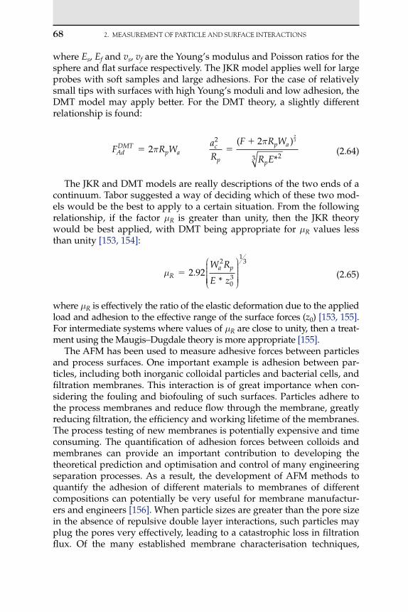
68 2. MEASUREMENTOFPARTICLEANdSURFACEINTERACTIONS
where Es, Ef and vs, vf are the Young’s modulus and Poisson ratios for the sphere and flat surface respectively. The JKR model applies well for large probes with soft samples and large adhesions. For the case of relatively small tips with surfaces with high Young’s moduli and low adhesion, the DMT model may apply better. For the DMT theory, a slightly different relationship is found:
F R WaR
F R W
R EAdDMT
p ac
p
p a
p
222
23
23
ππ( )
*
(2.64)
The JKR and DMT models are really descriptions of the two ends of a continuum. Tabor suggested a way of deciding which of these two mod-els would be the best to apply to a certain situation. From the following relationship, if the factor R is greater than unity, then the JKR theory would be best applied, with DMT being appropriate for R values less than unity [153, 154]:
Ra pW R
E z 2 92
2
03
13
.*
(2.65)
where R is effectively the ratio of the elastic deformation due to the applied load and adhesion to the effective range of the surface forces (z0) [153, 155]. For intermediate systems where values of R are close to unity, then a treat-ment using the Maugis–Dugdale theory is more appropriate [155].
The AFM has been used to measure adhesive forces between particles and process surfaces. One important example is adhesion between par-ticles, including both inorganic colloidal particles and bacterial cells, and filtration membranes. This interaction is of great importance when con-sidering the fouling and biofouling of such surfaces. Particles adhere to the process membranes and reduce flow through the membrane, greatly reducing filtration, the efficiency and working lifetime of the membranes. The process testing of new membranes is potentially expensive and time consuming. The quantification of adhesion forces between colloids and membranes can provide an important contribution to developing the theoretical prediction and optimisation and control of many engineering separation processes. As a result, the development of AFM methods to quantify the adhesion of different materials to membranes of different compositions can potentially be very useful for membrane manufactur-ers and engineers [156]. When particle sizes are greater than the pore size in the absence of repulsive double layer interactions, such particles may plug the pores very effectively, leading to a catastrophic loss in filtration flux. Of the many established membrane characterisation techniques,

2.4 AdHESIONFORCESMEASUREdByAFM 69
only the colloid probe method can measure the adhesive forces between particles and membrane surfaces and hence allow prediction of the mem-brane fouling properties of the particles. In addition, the ability to make measurements in liquid allows the matching of observation conditions to those that occur in practice.
Studies have also been carried out on the adhesion forces between calcium carbonate crystals and stainless steel surfaces. The adhesion of CaCO3 to steel process equipment surfaces plays an important role in the formation of scale deposits in desalination plant equipment, as well as in domestic appliances such as kettles and other household appliances. Al-Anezi et al. [157] measured the adhesion between CaCO3 probes and stain-less steel surfaces of different grades of roughness. In Figure 2.7 is an SEM image showing an example of a CaCO3 crystal mounted on an AFM canti-lever. The roughest surface had the lowest adhesion than the two smoother surfaces examined. The effect of liquid environment was also examined. Adhesive forces measured in sea water to which 2 ppm of an anti-scaling agent had been added were significantly more reduced than when mea-sured in sea water alone. In addition, the proportion of measured force curves that showed no observable adhesion rose from 1% of all obtained force curves in sea water to 57% with the addition of the anti-scale agent.
FIGuRE 2.7 SEM image of a CaCO3 crystal mounted upon an AFM cantilever for use in determining adhesion with stainless steel surfaces.

70 2. MEASUREMENTOFPARTICLEANdSURFACEINTERACTIONS
2.5 EFFECt oF RouGHnESS on MEASuREd AdHESIon And SuRFACE FoRCES
The continuum theories outlined above, such as the JKR and DMT theories, assume that perfectly smooth surfaces come into contact [2]. Unfortunately, the degree of roughness of particles and surfaces is quite variable, and often, except for when studying molecularly smooth sur-faces, some account may be needed to be taken of roughness. The pres-ence of asperities on surfaces coming into contact serves, in most cases, to effectively decrease the contact area. There are a number of models that have been developed to account for the effect of surface roughness on measured adhesion when trying to infer various properties of interac-tions from adhesion forces. These generally use some measure of rough-ness, such as the root mean square (rms) roughness of the surface, or values for mean asperity size to account for the reduced contact areas due to the presence of surface asperities [158–165]. As well as serving to keep the two surfaces separated, the angle at which asperities on the particle surfaces approach each other may also affect the effective contact area and thus the measured adhesion [166]. Rabinovich et al. [162] deter-mined that surface roughness values as small as 1.6 nm rms were signifi-cant and could reduce adhesion values by as much as fivefold from that expected.
In addition, rough particles make determination of the radius of probe particles, and hence normalisation by particle size, difficult. Larson and colleagues [167] determined an effective probe radius when performing measurements between TiO2 colloids and crystal surfaces by fitting force data to an electrical double layer model, with surface potential values determined independently. This allowed calculation of an effective probe radius that was used to normalise all subsequent force measurements.
AbbREVIAtIonS And SyMbolS
a Effective hard sphere particle radius in solution mac Contact radius mai Particle radius of molecule i MaVW van der Waals gas constant N m4 mol2
A131 Effective Hamaker constant in medium 3 JAH Hamaker constant (in vacuum or in medium) JbVW van der Waals gas constant m3 mol1
c Velocity of light in a vacuum (2.998 108) m s1

ABBREvIATIONSANdSyMBOLS 71
C Capacitance C V1
CD Debye interaction constant J m6
CK Keesom interaction constant J m6
CL London interaction constant J m6
CT Interaction constant J m6
CUV Cauchy Plot parameter
d Distance to OHP (surface of shear) mD Surface to surface separation distance mDjtc Jump-in distance mD0 Characteristic decay length me Elementary charge (1.602 1019) CE* Reduced Young’s modulus Pa s2
Es Young’s modulus for the sphere PaEf Young’s modulus for the flat surface Paf0 Force extrapolated to separation distance, D 0 NF Force between surfaces/particles NFAd
JKR Adhesion pull-off force (JKR model) N
FAdDMT Adhesion pull-off force (DMT model) N
FH Hydrodynamic force for a sphere approaching a plane surface
N
FR Repulsive interparticle force NFSOL Hydration force Nh Planck’s constant (6.626 1034) m2 kg s1
h Planck’s constant divided by 2 (6.626 1034/2)
J s rad1
k Boltzmann constant (1.380 1023) J K1
kc Spring constant of the cantilever N m1
keff Effective spring constant of the cantilever-sample system
N m1
ks Stiffness of the sample N m1
K Constant in force equation NKi Equilibrium constant for ionisation reaction i Ml Correlation length of the orientational ordering
of water moleculesm
n Number of gas molecules mol
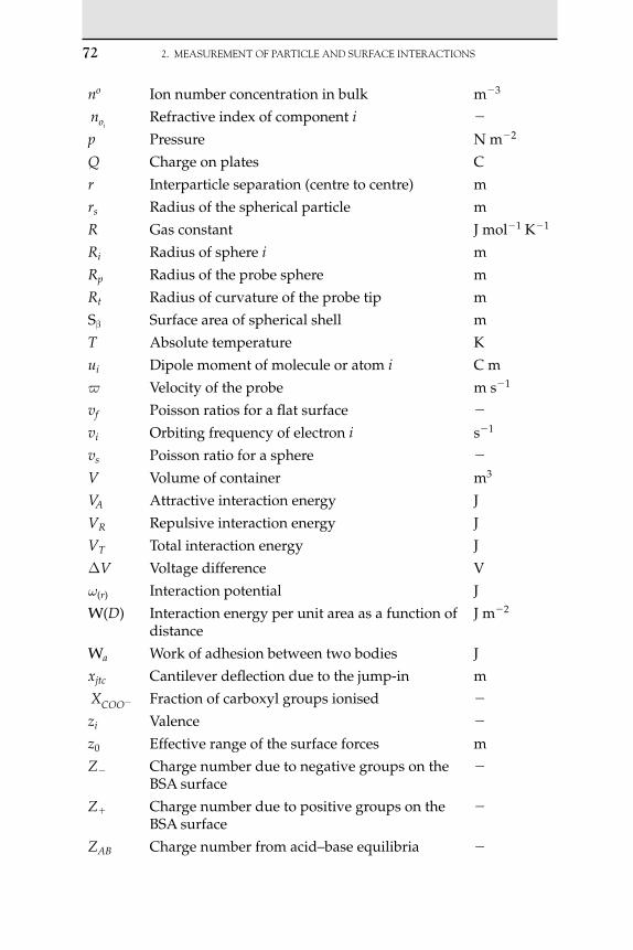
72 2. MEASUREMENTOFPARTICLEANdSURFACEINTERACTIONS
no Ion number concentration in bulk m3
noiRefractive index of component i
p Pressure N m2
Q Charge on plates C
r Interparticle separation (centre to centre) m
rs Radius of the spherical particle m
R Gas constant J mol1 K1
Ri Radius of sphere i m
Rp Radius of the probe sphere m
Rt Radius of curvature of the probe tip m
S Surface area of spherical shell m
T Absolute temperature K
ui Dipole moment of molecule or atom i C m
v Velocity of the probe m s1
vf Poisson ratios for a flat surface
vi Orbiting frequency of electron i s1
vs Poisson ratio for a sphere
V Volume of container m3
VA Attractive interaction energy J
VR Repulsive interaction energy J
VT Total interaction energy J
V Voltage difference V
w(r) Interaction potential J
W(D) Interaction energy per unit area as a function of distance
J m2
Wa Work of adhesion between two bodies J
xjtc Cantilever deflection due to the jump-in m
XCOOˆ Fraction of carboxyl groups ionised
zi Valence
z0 Effective range of the surface forces m
Z Charge number due to negative groups on the BSA surface
Z Charge number due to positive groups on the BSA surface
ZAB Charge number from acid–base equilibria
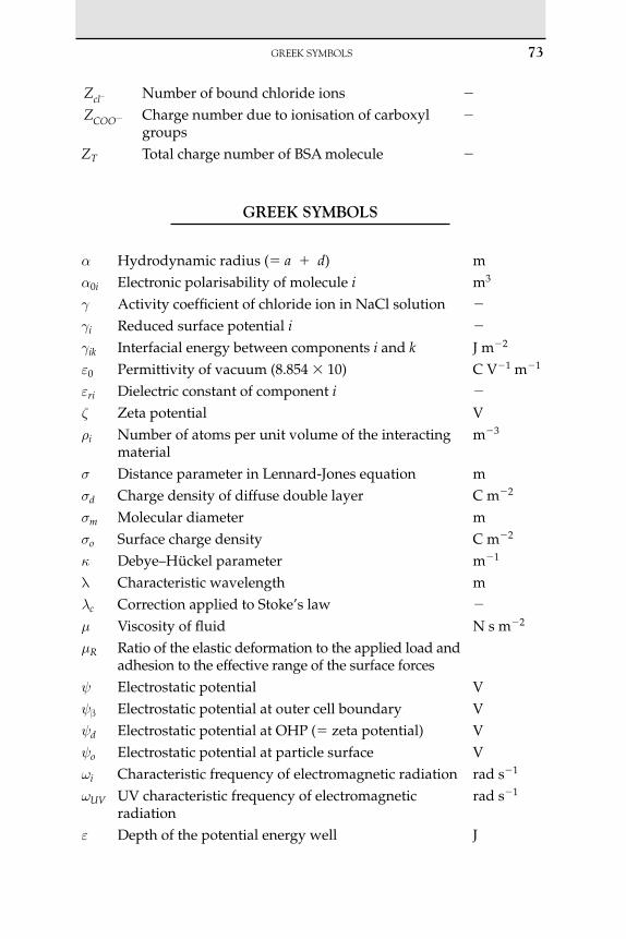
GREEkSyMBOLS 73
Zcl Number of bound chloride ions
ZCOOˆ Charge number due to ionisation of carboxyl groups
ZT Total charge number of BSA molecule
GREEk SyMbolS
Hydrodynamic radius ( a d) m0i Electronic polarisability of molecule i m3
Activity coefficient of chloride ion in NaCl solution
i Reduced surface potential i
ik Interfacial energy between components i and k J m2
ε0 Permittivity of vacuum (8.854 10) C V1 m1
εri Dielectric constant of component i
Zeta potential Vi Number of atoms per unit volume of the interacting
materialm3
Distance parameter in Lennard-Jones equation md Charge density of diffuse double layer C m2
m Molecular diameter mo Surface charge density C m2
Debye–Hückel parameter m1
Characteristic wavelength mc Correction applied to Stoke’s law
Viscosity of fluid N s m2
R Ratio of the elastic deformation to the applied load and adhesion to the effective range of the surface forces
Electrostatic potential V Electrostatic potential at outer cell boundary Vd Electrostatic potential at OHP ( zeta potential) Vo Electrostatic potential at particle surface Vwi Characteristic frequency of electromagnetic radiation rad s1
wUV UV characteristic frequency of electromagnetic radiation
rad s1
ε Depth of the potential energy well J
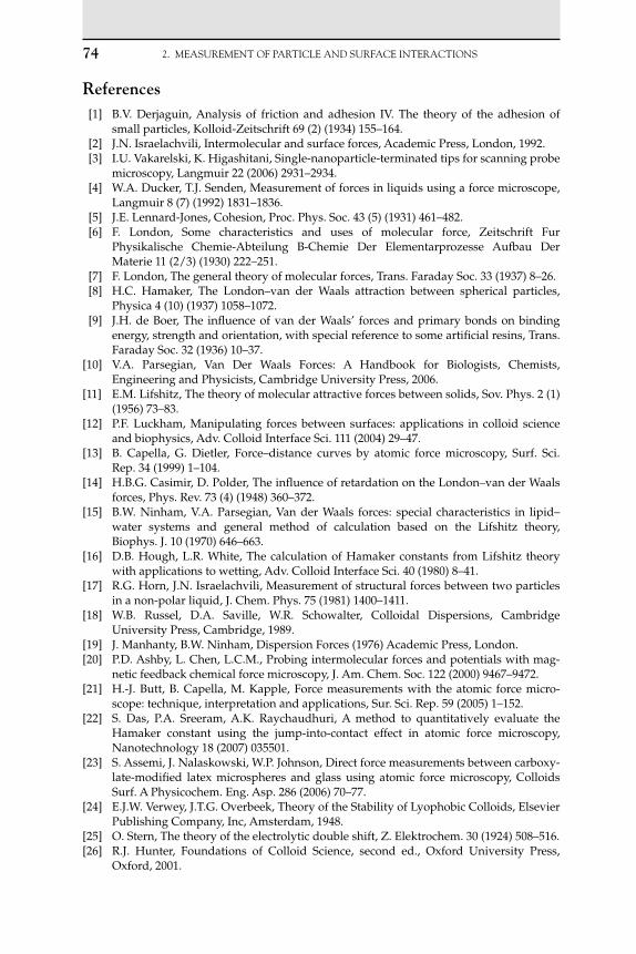
74 2. MEASUREMENTOFPARTICLEANdSURFACEINTERACTIONS
References [1] B.V. Derjaguin, Analysis of friction and adhesion IV. The theory of the adhesion of
small particles, Kolloid-Zeitschrift 69 (2) (1934) 155–164. [2] J.N. Israelachvili, Intermolecular and surface forces, Academic Press, London, 1992. [3] I.U. Vakarelski, K. Higashitani, Single-nanoparticle-terminated tips for scanning probe
microscopy, Langmuir 22 (2006) 2931–2934. [4] W.A. Ducker, T.J. Senden, Measurement of forces in liquids using a force microscope,
Langmuir 8 (7) (1992) 1831–1836. [5] J.E. Lennard-Jones, Cohesion, Proc. Phys. Soc. 43 (5) (1931) 461–482. [6] F. London, Some characteristics and uses of molecular force, Zeitschrift Fur
Physikalische Chemie-Abteilung B-Chemie Der Elementarprozesse Aufbau Der Materie 11 (2/3) (1930) 222–251.
[7] F. London, The general theory of molecular forces, Trans. Faraday Soc. 33 (1937) 8–26. [8] H.C. Hamaker, The London–van der Waals attraction between spherical particles,
Physica 4 (10) (1937) 1058–1072. [9] J.H. de Boer, The influence of van der Waals’ forces and primary bonds on binding
energy, strength and orientation, with special reference to some artificial resins, Trans. Faraday Soc. 32 (1936) 10–37.
[10] V.A. Parsegian, Van Der Waals Forces: A Handbook for Biologists, Chemists, Engineering and Physicists, Cambridge University Press, 2006.
[11] E.M. Lifshitz, The theory of molecular attractive forces between solids, Sov. Phys. 2 (1) (1956) 73–83.
[12] P.F. Luckham, Manipulating forces between surfaces: applications in colloid science and biophysics, Adv. Colloid Interface Sci. 111 (2004) 29–47.
[13] B. Capella, G. Dietler, Force–distance curves by atomic force microscopy, Surf. Sci. Rep. 34 (1999) 1–104.
[14] H.B.G. Casimir, D. Polder, The influence of retardation on the London–van der Waals forces, Phys. Rev. 73 (4) (1948) 360–372.
[15] B.W. Ninham, V.A. Parsegian, Van der Waals forces: special characteristics in lipid–water systems and general method of calculation based on the Lifshitz theory, Biophys. J. 10 (1970) 646–663.
[16] D.B. Hough, L.R. White, The calculation of Hamaker constants from Lifshitz theory with applications to wetting, Adv. Colloid Interface Sci. 40 (1980) 8–41.
[17] R.G. Horn, J.N. Israelachvili, Measurement of structural forces between two particles in a non-polar liquid, J. Chem. Phys. 75 (1981) 1400–1411.
[18] W.B. Russel, D.A. Saville, W.R. Schowalter, Colloidal Dispersions, Cambridge University Press, Cambridge, 1989.
[19] J. Manhanty, B.W. Ninham, Dispersion Forces (1976) Academic Press, London. [20] P.D. Ashby, L. Chen, L.C.M., Probing intermolecular forces and potentials with mag-
netic feedback chemical force microscopy, J. Am. Chem. Soc. 122 (2000) 9467–9472. [21] H.-J. Butt, B. Capella, M. Kapple, Force measurements with the atomic force micro-
scope: technique, interpretation and applications, Sur. Sci. Rep. 59 (2005) 1–152. [22] S. Das, P.A. Sreeram, A.K. Raychaudhuri, A method to quantitatively evaluate the
Hamaker constant using the jump-into-contact effect in atomic force microscopy, Nanotechnology 18 (2007) 035501.
[23] S. Assemi, J. Nalaskowski, W.P. Johnson, Direct force measurements between carboxy-late-modified latex microspheres and glass using atomic force microscopy, Colloids Surf. A Physicochem. Eng. Asp. 286 (2006) 70–77.
[24] E.J.W. Verwey, J.T.G. Overbeek, Theory of the Stability of Lyophobic Colloids, Elsevier Publishing Company, Inc, Amsterdam, 1948.
[25] O. Stern, The theory of the electrolytic double shift, Z. Elektrochem. 30 (1924) 508–516. [26] R.J. Hunter, Foundations of Colloid Science, second ed., Oxford University Press,
Oxford, 2001.

REFERENCES 75
[27] G.M. Bell, S. Levine, L.N. McCartney, Approximate methods of determining the double- layer free energy of interaction between two charged colloidal spheres, J. Colloid Interface Sci. 33 (3) (1970) 335–359.
[28] J. Gregory, Interaction of unequal double layers at constant charge, J. Colloid Interface Sci. 51 (1975) 44–51.
[29] R.I. Hogg, T.W. Healey, D.W. Fuerstenau, Mutual coagulation of colloidal dispersions, Trans. Faraday Soc. 62 (1966) 1638–1651.
[30] G.R. Wiese, T.W. Healy, Effect of particle size on colloid stability, Trans. Faraday Soc. 66 (1970) 490–500.
[31] H. Ohshima, T. Kondo, Comparison of three models on double layer interaction, J. Colloid Interface Sci. 126 (1988) 382–383.
[32] G. Kar, S. Chander, T.S. Mika, The potential energy of interaction between dissimilar electrical double layers, J. Colloid Interface Sci. 44 (1973) 347–355.
[33] L.N. McCartney, S. Levine, An improvement on Derjaguin’s expression at small potentials for the double-layer interaction energy of two spherical colloidal particles, J. Colloid Interface Sci. 30 (1969) 345–354.
[34] H. Muller, Zur Theorie der elektrischen Ladung und der Koagulation der Kolloide, Kolloidchemische Beihefte 26 (1928) 257.
[35] N.E. Hoskin, Solution to the Poisson–Boltzmann equation for the potential distribution in the double layer of a single spherical colloidal particle, Trans. Faraday Soc. 49 (1953) 1471.
[36] A.L. Loeb, P.H. Weirsema, J.T.G. Overbeek, The electrical double layer around a spher-ical colloid particle, MIT Press, Cambridge Mass, 1961.
[37] W.R. Bowen, F. Jenner, Dynamic ultrafiltration model for charged colloidal disper-sions: a Wigner–Seitz cell approach, Chem. Eng. Sci. 50 (1995) 1707.
[38] W.R. Bowen, A.O. Sharif, Adaptive finite-element solution of the nonlinear Poisson–Boltzmann equation: a charged spherical particle at various distances from a charged cylindrical pore in a charged planar surface, J. Colloid Interface Sci. 187 (1997) 363.
[39] J.J. Gray, B. Chiang, R.T. Bonnecaze, Colloidal particles: origin of anomalous multi-body interactions, Nature 402 (1999) 705.
[40] N.E. Hoskin, The interaction of 2 identical spherical colloidal particles. 1. Potential distribution, Philos. Trans. R. Soc. (Lond.) A 248 (1956) 433.
[41] J.E. Ledbetter, T.L. Croxton, D.A. McQuarrie, The interaction of two charged spheres in the Poisson–Boltzmann equation, Can. J. Chem. 59 (1981) 1860.
[42] C.W. Outhwaite, P. Molero, Effective interaction between colloidal particles using a symmetric Poisson–Boltzmann theory, Chem. Phys. Lett. 197 (1992) 643–648.
[43] J.E. Sanchez-Sanchez, M. Lozada-Cassou, Exact numerical solution to the integral equation version of the Poisson–Boltzmann equation of two interacting spherical col-loidal particles. Chem. Phys. Lett. (190) (1992) 202–208.
[44] M. Strauss, T.A. Ring, H.K. Bowen, Osmotic pressure for concentrated suspensions of polydisperse particles with thick double layers, J. Colloid Interface Sci. 118 (1987) 326–334.
[45] W.R. Bowen, P.M. Williams, Finite difference solution of the 2-dimensional Poisson–Boltzmann equation for spheres in confined geometries, Colloids Surf. A Physicochem. Eng. Asp. 204 (2002) 103–115.
[46] M. Ospeck, S. Fraden solving the Poisson–Boltzmann equation to obtain information energies between confined, like-charged cylinders, J. Chem. Phys. 109 (1998) 9166.
[47] W.R. Bowen, P.M. Williams, Dynamic ultafiltration model for proteins: a colloidal interaction approach, Biotechnol. Bioeng. 50 (2) (1996) 125–135.
[48] B.W. Ninham, V.A. Parsegian, Electrostatic potential between surfaces bearing ioniz-able groups in ionic equilibrium with physiological saline solution, J. Theor. Biol. 31 (1971) 405–428.
[49] J.R. Brown, P. Shockley. In: P. Jost, H. Griffiths (Eds.), Lipid–Protein Interactions, New York, Wiley, 1982, p. 25.
[50] C. Tanford, S.A. Swanson, W.S. Shore, Hydrogen ion equilibria of bovine serum albu-min, J. Am. Chem. Soc. 77 (1955) 6414.

76 2. MEASUREMENTOFPARTICLEANdSURFACEINTERACTIONS
[51] R.C. Cantor, P.R. Schimmel, Biophysical Chemistry. Part II – Techniques for the Study of Biological Structure and Function, Freeman and Company, New York, 1980.
[52] G. Scatchard, E.S. Black, The effect of salts on the isoionic and isoelectric points of proteins, J. Phys. Colloid Chem. 53 (1949) 88.
[53] W.R. Bowen, P.M. Williams, The osmotic pressure of electrostatically stabilized colloi-dal dispersions, J. Colloid Interface Sci. 184 (1996) 241.
[54] T.W. Healy, L.E. White, Ionizable surface group models of aqueous interfaces, Adv. Colloid Interface Sci. 9 (1978) 303.
[55] R.A. Serway, Physics for Scientists and Engineers with Modern Physics, 3rd ed, Updated Version, Chicago, Saunders College Publishing, 1992, p. 714.
[56] R.J. Hunter, Zeta Potential in Colloid Science, Academic Press, London, 1981. [57] S. Kuwabara, The forces experienced by randomly distributed parallel circular cylin-
ders or spheres in a viscous flow at small Reynolds number, J. Physical Soc. Japan 14 (4) (1959) 527–532.
[58] E.S. Reiner, C.J. Radke, Electrostatic interactions in colloidal suspensions – tests of pairwise additivity, AIChE J. 37 (6) (1991) 805–824.
[59] N.E. Hoskin, S. Levine, The interaction of two identical spherical colloidal particles: II. The free energy, Philos. Trans. R. Soc. (Lond.) A 248 (951) (1956) 449–466.
[60] L. Guldbrand, L.G. Nilsson, L.A. Nordenskiöld, Monte Carlo simulation study of elec-trostatic forces between hexagonally packed DNA double helices, J. Chem. Phys. 85 (1986) 6687–6698.
[61] E. Wigner, F. Seitz, On the constitution of metallic sodium, Phys. Rev. 43 (10) (1933) 804–810.
[62] B.V. Derjaguin, L.D. Landau, Theory of the stability of strongly charged lyophobic sols and of the adhesion of strongly charged particles in solutions of electrolytes, Acta Physicochim. URSS 14 (1941) 633.
[63] A.E. Larsen, D.G. Grier, Like-charge attractions in metastable colloidal crystallites, Nature 385 (1997) 230–233.
[64] N. Ise, T. Okubo, M. Sugimura, K. Ito, H.J. Nolte, Ordered structure in dilute solutions of highly charge polymers lattices as studied by microscopy. I. Interparticle distance as a function of latex concentration, J. Chem. Phys. 78 (1983) 536–540.
[65] J.C. Crocker, D.G. Grier, Microscopic measurements of pair interaction potential of charge stabilised colloid, Phys. Rev. Lett. 73 (1994) 352–355.
[66] D.G. Grier, Optical tweezers in colloid and interface science, Curr. Opin. Colloid Interface Sci. 2 (1997) 264–270.
[67] T.M. Squires, M.P. Brenner, Like-charge attraction and hydrodynamic interaction, Phys. Rev. Lett. 85 (23) (2000) 4976–4979.
[68] H.-J. Butt, R. Berger, E. Bonnacurso, Y. Chen, J. Wang, Impact of atomic force micros-copy on interface and colloid science, Adv. Colloid Interface Sci. (2007).
[69] J. Ralston, I. Larson, M.W. Rutland, A.A. Feiler, M. Kleijn, Atomic force microscopy and direct surface force measurements (IUPAC technical report), Pure Appl. Chem. 77 (2005) 2149–2170.
[70] D.J. Johnson, N.J. Miles, N. Hilal, Quantification of particle–bubble interactions using atomic force microscopy: a review, Adv. Colloid Interface Sci. 127 (2) (2006) 67–81.
[71] W.A. Ducker, T.J. Senden, R.M. Pashley, Direct measurement of colloidal forces using an atomic force microscope, Nature 353 (1991) 239–241.
[72] A. Milling, P. Mulvaney, I. Larson, Direct measurement of repulsive van der Waals interactions using an atomic force microscope, J. Colloid Interface Sci. 180 (1996) 460–465.
[73] M.E. Karaman, R.M. Pashley, T.D. Waite, S.J. Hatch, H. Bustamante, A comparison of the interaction forces between model alumina surfaces and their colloidal properties, Colloids Surf. A Physicochem. Eng. Asp. 129–130 (1997) 239–255.
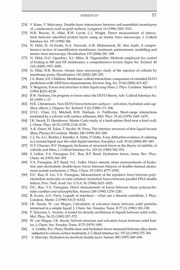
REFERENCES 77
[74] V. Kane, P. Mulvaney, Double-layer interactions between self-assembled monolayers of -undecanoic acid on gold surfaces, Langmuir 14 (1998) 3303–3311.
[75] W.R. Bowen, N. Hilal, R.W. Lovitt, C.J. Wright, Direct measurement of interac-tions between adsorbed protein layers using an atomic force microscope, J. Colloid Interface Sci. 197 (1998) 348.
[76] N. Hilal, H. Al-Zoubi, N.A. Darwish, A.W. Mohammed, M. Abu Arabi, A compre-hensive review of nanofiltration membranes: treatment, pretreatment, modelling and atomic force microscopy, Desalination 170 (2004) 281–308.
[77] N. Hilal, O.O. Ogunbiyi, N.J. Miles, R. Nigmatullin, Methods employed for control of fouling in MF and NF membranes: a comprehensive review, Separ. Sci. Technol. 40 (10) (2005) 1957–2005.
[78] N. Hilal, W.R. Bowen, Atomic force microscopy study of the rejection of colloids by membrane pores, Desalination 150 (2002) 289–295.
[79] J.A. Brant, A.E. Childress, Membrane–colloid interactions: comparison of extended DLVO predictions with AFM force measurements, Environ. Eng. Sci. 19 (6) (2002) 413–427.
[80] V. Bergeron, Forces and structure in thin liquid soap films, J. Phys. Condens. Matter 11 (1999) R215–R238.
[81] B.W. Ninham, On progress in forces since the DLVO theory, Adv. Colloid Interface Sci. 83 (1999) 1–17.
[82] H.K. Christenson, Non-DLVO forces between surfaces – solvation, hydration and cap-illary effects, J. Dispers. Sci. Technol. 9 (2) (1988) 171–206.
[83] D.Y.C. Chan, D.J. Mitchell, B.W. Ninham, A. Pailthorpe, Short-range interactions mediated by a solvent with surface adhesion, Mol. Phys. 35 (6) (1978) 1669–1679.
[84] I.K. Snook, D. Henderson, Monte–Carlo study of a hard-sphere fluid near a hard wall, J. Chem. Phys. 68 (5) (1978) 2134–2139.
[85] A.K. Doerr, M. Tolan, T. Seydel, W. Press, The interface structure of thin liquid hexane films, Physica B Condens. Matter 248 (1998) 263–268.
[86] C.J. Yu, A.G. Richter, J. Kmetko, A. Datta, P. Dutta, X-ray diffraction evidence of ordering in a normal liquid near the solid–liquid interface, Europhys. Lett. 50 (4) (2000) 487–493.
[87] N.V. Churaev, B.V. Derjaguin, Inclusion of structural forces in the theory of stability of colloids and films, J. Colloid Interface Sci. 103 (2) (1985) 542–553.
[88] S. Leikin, V.A. Parsegian, D.C. Rau, R.P. Rand, Hydration forces, Annu. Rev. Phys. Chem. 44 (1993) 369–395.
[89] V.A. Parsegian, R.P. Rand, N.L. Fuller, Direct osmotic stress measurements of hydra-tion and electrostatic double-layer forces between bilayers of double-chained ammo-nium acetate surfactants, J. Phys. Chem. 95 (1991) 4777–4782.
[90] D.C. Rau, B. Lee, V.A. Parsegian, Measurement of the repulsive force between poly-electrolyte molecules in ionic solution: hydration forces between parallel DNA double helices, Proc. Natl. Acad. Sci. U.S.A. 81 (1984) 2621–2625.
[91] D.C. Rau, V.A. Parsegian, Direct measurement of forces between linear polysaccha-rides xanthan and schizophyllan, Science 249 (1990) 1278–1281.
[92] R. Evans, A.O. Parry, Liquids at interfaces – what can a theorist contribute, J. Phys. Condens. Matter 2 (1990) SA15–SA32.
[93] I.K. Snook, W. van Megen, Calculation of solvation forces between solid particles immersed in a simple liquid, J. Chem. Soc. Faraday Trans. II 77 (1) (1981) 181–190.
[94] P. Tarazona, L. Vicente, A model for density oscillations in liquids between solid walls, Mol. Phys. 56 (3) (1985) 557–572.
[95] W. van Megan, I.K. Snook, Solvent structure and solvation forces between solid bod-ies, J. Chem. Soc. Faraday Trans. II 75 (1979) 1095.
[96] A. Grabbe, R.G. Horn, Double-layer and hydration forces measured between silica sheets subjected to various surface treatments, J. Colloid Interface Sci. 157 (2) (1993) 375–383.
[97] S. Marcelja, Hydration in electrical double layer, Nature 385 (1997) 689–690.

78 2. MEASUREMENTOFPARTICLEANdSURFACEINTERACTIONS
[98] E. Ruckenstein, M. Manciu, The coupling between the hydration and double layer interactions, Langmuir 18 (2002) 7584–7593.
[99] S. Leikin, A.A. Kornyshev, Theory of hydration forces. Nonlocal electrostatic interac-tion of neutral surfaces, J. Chem. Phys. 92 (11) (1990) 6890–6898.
[100] J. Israelachvili, H. Wennerström, Role of hydration and water structure in biological and colloidal interactions, Nature 379 (1996) 219–225.
[101] D. Leckband, J. Israelachvili, Intermolecular forces in biology, Q. Rev. Biophys. 34 (2) (2001) 105–267.
[102] J.N. Israelachvili, H. Wennerström, Hydration or steric forces between amphiphilic surfaces? Langmuir 6 (1990) 873–876.
[103] J. Faraudo, F. Bresme, Origin of the short-range, strong repulsive force between ionic surfactant layers, Phys. Rev. Lett. 94 (7) (2005) 077802.
[104] J. Faraudo, F. Bresme, Anomalous dielectric behavior of water in ionic Newton black films, Phys. Rev. Lett. 92 (2004) 236102.
[105] D.W.R. Gruen, S. Marcelja, Spatially varying polarization in water, J. Chem. Soc. Faraday Trans. 2 79 (1983) 225–242.
[106] S.J. O’Shea, M.E. Welland, T. Rayment, Solvation forces near a graphite surface meas-ured, Appl. Phys. Lett. 60 (19) (1992) 2356–2358.
[107] R. Lim, S.F.Y. Li, S.J. O’Shea, Solvation forces using sample-modulation atomic force microscopy, Langmuir 18 (2002) 6116–6124.
[108] L.T.W. Lim, A.T.S. Wee, S.J. O’Shea, Effect of tip size on force measurement in atomic force microscopy, Langmuir (2008).
[109] S.J. O’Shea, M.E. Welland, Atomic force microscopy at solid–liquid interfaces, Langmuir 14 (1998) 4186–4197.
[110] V. Franz, H.-J. Butt, Confined liquids: solvation forces in liquid alcohols between solid surfaces, J. Phys. Chem. B 106 (2002) 1703–1708.
[111] J.J. Valle-Delgado, J.A. Molina-Bolivar, F. Galisteo-Gonzalez, M.J. Galvez-Ruiz, A. Feiler, M.W. Rutland, Hydration forces between silica surfaces: experimental data and predictions from different theories, J. Chem. Phys. 123 (3) (2005) 034708.
[112] S.P. Jarvis, T. Uchihashi, T. Ishida, H. Tokumoto, Y. Nakayama, Local solvation shell measurement in water using a carbon nanotube probe, J. Phys. Chem. B 104 (26) (2000) 6091–6094.
[113] J. Israelachvili, R.M. Pashley, Molecular layering of water at surface and origin of repulsive hydration forces, Nature 306 (1983) 249–250.
[114] P.G. de Gennes, Polymers at an interface: a simplified view, Adv. Colloid Interface Sci. 27 (1987) 189–209.
[115] F.T. Hesselin, Theory of stabilization of dispersions by adsorbed macromolecules. 1. Statistics of change of some configurational properties of adsorbed macromolecules on approach of an impenetrable interface, J. Phys. Chem. 75 (1) (1971) 65.
[116] A. Vrij, Polymers at interfaces and interactions in colloidal dispersions, Pure Appl. Chem. 48 (4) (1976) 471–483.
[117] S.T. Milner, T.A. Witten, M.E. Cates, Theory of the grafted polymer brush, Macromolecules 21 (8) (1988) 2610–2619.
[118] K. Ingersent, J. Klein, P. Pincus, Interactions between surfaces with adsorbed polymers – poor solvent. 2. Calculations and comparison with experiment, Macromolecules 19 (5) (1986) 1374–1381.
[119] K. Ingersent, J. Klein, P. Pincus, Forces between surfaces with adsorbed polymers – theta solvent. 3. Calculations and comparison with experiment, Macromolecules 23 (2) (1990) 548–560.
[120] J.N. Israelachvili, M. Tirrell, J. Klein, Y. Almog, Forces between 2 layers of adsorbed polystyrene immersed in cyclohexane below and above the theta-temperature, Macromolecules 17 (1984) 204.
[121] J.W. Cahn, Critical point wetting, J. Chem. Phys. 66 (1977) 3667.
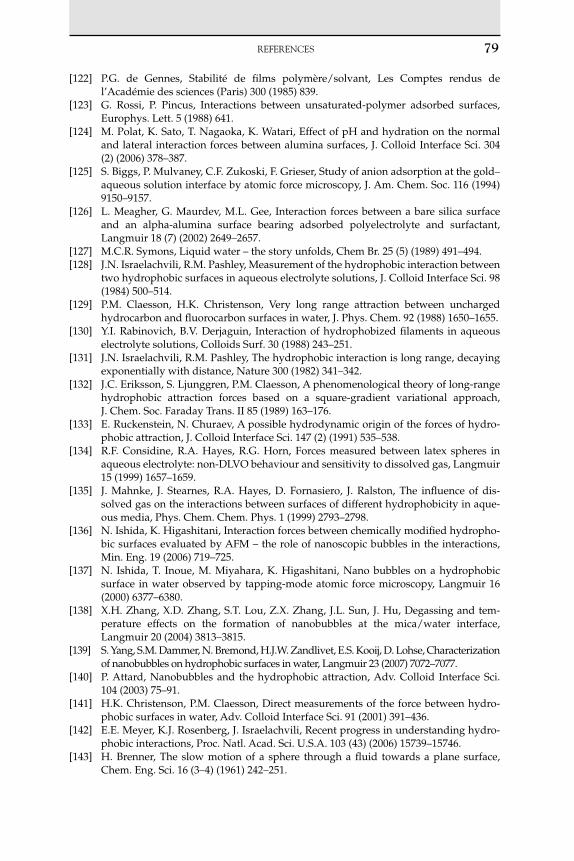
REFERENCES 79
[122] P.G. de Gennes, Stabilité de films polymère/solvant, Les Comptes rendus de l’Académie des sciences (Paris) 300 (1985) 839.
[123] G. Rossi, P. Pincus, Interactions between unsaturated-polymer adsorbed surfaces, Europhys. Lett. 5 (1988) 641.
[124] M. Polat, K. Sato, T. Nagaoka, K. Watari, Effect of pH and hydration on the normal and lateral interaction forces between alumina surfaces, J. Colloid Interface Sci. 304 (2) (2006) 378–387.
[125] S. Biggs, P. Mulvaney, C.F. Zukoski, F. Grieser, Study of anion adsorption at the gold–aqueous solution interface by atomic force microscopy, J. Am. Chem. Soc. 116 (1994) 9150–9157.
[126] L. Meagher, G. Maurdev, M.L. Gee, Interaction forces between a bare silica surface and an alpha-alumina surface bearing adsorbed polyelectrolyte and surfactant, Langmuir 18 (7) (2002) 2649–2657.
[127] M.C.R. Symons, Liquid water – the story unfolds, Chem Br. 25 (5) (1989) 491–494. [128] J.N. Israelachvili, R.M. Pashley, Measurement of the hydrophobic interaction between
two hydrophobic surfaces in aqueous electrolyte solutions, J. Colloid Interface Sci. 98 (1984) 500–514.
[129] P.M. Claesson, H.K. Christenson, Very long range attraction between uncharged hydrocarbon and fluorocarbon surfaces in water, J. Phys. Chem. 92 (1988) 1650–1655.
[130] Y.I. Rabinovich, B.V. Derjaguin, Interaction of hydrophobized filaments in aqueous electrolyte solutions, Colloids Surf. 30 (1988) 243–251.
[131] J.N. Israelachvili, R.M. Pashley, The hydrophobic interaction is long range, decaying exponentially with distance, Nature 300 (1982) 341–342.
[132] J.C. Eriksson, S. Ljunggren, P.M. Claesson, A phenomenological theory of long-range hydrophobic attraction forces based on a square-gradient variational approach, J. Chem. Soc. Faraday Trans. II 85 (1989) 163–176.
[133] E. Ruckenstein, N. Churaev, A possible hydrodynamic origin of the forces of hydro-phobic attraction, J. Colloid Interface Sci. 147 (2) (1991) 535–538.
[134] R.F. Considine, R.A. Hayes, R.G. Horn, Forces measured between latex spheres in aqueous electrolyte: non-DLVO behaviour and sensitivity to dissolved gas, Langmuir 15 (1999) 1657–1659.
[135] J. Mahnke, J. Stearnes, R.A. Hayes, D. Fornasiero, J. Ralston, The influence of dis-solved gas on the interactions between surfaces of different hydrophobicity in aque-ous media, Phys. Chem. Chem. Phys. 1 (1999) 2793–2798.
[136] N. Ishida, K. Higashitani, Interaction forces between chemically modified hydropho-bic surfaces evaluated by AFM – the role of nanoscopic bubbles in the interactions, Min. Eng. 19 (2006) 719–725.
[137] N. Ishida, T. Inoue, M. Miyahara, K. Higashitani, Nano bubbles on a hydrophobic surface in water observed by tapping-mode atomic force microscopy, Langmuir 16 (2000) 6377–6380.
[138] X.H. Zhang, X.D. Zhang, S.T. Lou, Z.X. Zhang, J.L. Sun, J. Hu, Degassing and tem-perature effects on the formation of nanobubbles at the mica/water interface, Langmuir 20 (2004) 3813–3815.
[139] S. Yang, S.M. Dammer, N. Bremond, H.J.W. Zandlivet, E.S. Kooij, D. Lohse, Characterization of nanobubbles on hydrophobic surfaces in water, Langmuir 23 (2007) 7072–7077.
[140] P. Attard, Nanobubbles and the hydrophobic attraction, Adv. Colloid Interface Sci. 104 (2003) 75–91.
[141] H.K. Christenson, P.M. Claesson, Direct measurements of the force between hydro-phobic surfaces in water, Adv. Colloid Interface Sci. 91 (2001) 391–436.
[142] E.E. Meyer, K.J. Rosenberg, J. Israelachvili, Recent progress in understanding hydro-phobic interactions, Proc. Natl. Acad. Sci. U.S.A. 103 (43) (2006) 15739–15746.
[143] H. Brenner, The slow motion of a sphere through a fluid towards a plane surface, Chem. Eng. Sci. 16 (3–4) (1961) 242–251.
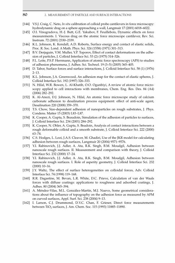
80 2. MEASUREMENTOFPARTICLEANdSURFACEINTERACTIONS
[144] V.S.J. Craig, C. Neto, In situ calibration of colloid probe cantilevers in force microscopy: hydrodynamic drag on a sphere approaching a wall, Langmuir 17 (2001) 6018–6022.
[145] O.I. Vinogradova, H.-J. Butt, G.E. Yakubov, F. Feuillebois, Dynamic effects on force measurements. I. Viscous drag on the atomic force microscope cantilever, Rev. Sci. Instrum. 72 (2001) 2330–2339.
[146] K.L. Johnson, K. Kendall, A.D. Roberts, Surface energy and contact of elastic solids, Proc. R. Soc. Lond. A Math. Phys. Sci. 324 (1558) (1971) 301–313.
[147] B.V. Derjaguin, V.M. Muller, Y.P. Toporov, Effect of contact deformations on the adhe-sion of particles, J. Colloid Interface Sci. 53 (2) (1975) 314–326.
[148] F.L. Leite, P.S.P. Herrmann, Application of atomic force spectroscopy (AFS) to studies of adhesion phenomena, J. Adhes. Sci. Technol. 19 (3–5) (2005) 365–405.
[149] D. Tabor, Surface forces and surface interactions, J. Colloid Interface Sci. 58 (1) (1976) 2–13.
[150] K.L. Johnson, J.A. Greenwood, An adhesion map for the contact of elastic spheres, J. Colloid Interface Sci. 192 (1997) 326–333.
[151] N. Hilal, W.R. Bowen, L. Al-Khatib, O.O. Ogunbiyi, A review of atomic force micro-scopy applied to cell interactions with membranes, Chem. Eng. Res. Des. 84 (A4) (2006) 282–292.
[152] K. Al-Anezi, D.J. Johnson, N. Hilal, An atomic force microscope study of calcium carbonate adhesion to desalination process equipment: effect of anti-scale agent, Desalination 220 (2008) 359–370.
[153] T.S. Chow, Size-dependent adhesion of nanoparticles on rough substrates, J. Phys. Condens. Matter 15 (2003) L83–L87.
[154] K. Cooper, A. Gupta, S. Beaudoin, Simulation of the adhesion of particles to surfaces, J. Colloid Interface Sci. 234 (2001) 284–292.
[155] K. Cooper, N. Ohler, A. Gupta, S. Beadoin, Analysis of contact interactions between a rough deformable colloid and a smooth substrate, J. Colloid Interface Sci. 222 (2000) 63–74.
[156] C.S. Hodges, L. Looi, J.A.S. Cleaver, M. Ghadiri, Use of the JKR model for calculating adhesion between rough surfaces, Langmuir 20 (2004) 9571–9576.
[157] Y.I. Rabinovich, J.J. Adler, A. Ata, R.K. Singh, B.M. Moudgil, Adhesion between nanoscale rough surfaces. II. Measurement and comparison with theory, J. Colloid Interface Sci. 232 (2000) 17–24.
[158] Y.I. Rabinovich, J.J. Adler, A. Ata, R.K. Singh, B.M. Moudgil, Adhesion between nanoscale rough surfaces. I. Role of asperity geometry, J. Colloid Interface Sci. 232 (2000) 10–16.
[159] J.Y. Waltz, The effect of surface heterogeneities on colloidal forces, Adv. Colloid Interface Sci. 74 (1998) 119–168.
[160] R.R. Dagastine, M. Bevan, L.R. White, D.C. Prieve, Calculation of van der Waals forces with diffuse coatings: applications to roughness and adsorbed coatings, J. Adhes. 80 (2004) 365–394.
[161] A. Méndez-Vilas, M.L. González-Martín, M.J. Nuevo, Some geometrical considera-tions about the influence of topography on the adhesion force as measured by AFM on curved surfaces, Appl. Surf. Sci. 238 (2004) 9–13.
[162] I. Larson, C.J. Drummond, D.Y.C. Chan, F. Grieser, Direct force measurements between TiO2 surfaces, J. Am. Chem. Soc. 115 (1993) 11885–11890.
O U T L I N E
3.1 Introduction 82
3.2 Particle–Bubble Interactions 82
3.3 Determination of Particle–Bubble Separation 86
3.4 Determination of Contact Angle from Force–Distance Curves 88
3.5 Effect of Surface Preparation on Particle–Bubble Interactions 913.5.1 Effect of Particle Surface Chemistry on Particle–Bubble Interactions 913.5.2 Effect of Surfactant on Particle–Bubble Interactions 94
3.6 Effect of Loading Force on Particle–Bubble Interactions 97
3.7 Effect of Hydrodynamics on Particle–Bubble Interactions 98
3.8 Conclusions 100
List of Abbreviations 101
List of Symbols 101References 102
QuantificationofParticle–Bubble
InteractionsUsingAtomicForceMicroscopy
Nidal Hilal and Daniel Johnson
3C H A P T E R
Atomic Force Microscopy in Process Engineering ©2009,ElsevierLtd81

82 3. QUANTIFICATIONOFPARTICLE–BUBBLEINTERACTIONs
3.1 IntroDuCtIon
The attachment of particles to bubbles in solution is of fundamental importance to several industrial processes most notably in froth flotation. Froth flotation is a significant industrial process, used primarily in the separation of mineral particles and also in the treatment of wastewater. The process of flotation involves the suspension of finely ground min-eral particles in a chamber through which large volumes of air or another gas are bubbled. Hydrophobic particles will attach more readily to air bubbles passing through the medium and will thus rise to the top of the chamber where they form froth at the surface and become separated from other materials. Hydrophilic particles, which are less able to attach to the air bubbles, will eventually sink to the bottom of the chamber. In addition, a number of additives, including surfactants, termed collectors, may also be introduced to increase the hydrophobicity of the particles of interest and consequently increase the efficiency or specificity of the flo-tation process [1, 2].
It follows that an understanding of the nature and strength of the inter-actions between colloidal particles suspended in solution and air bubbles is of fundamental importance to developing new ways of increasing flo-tation efficiency and modulating specificity. Atomic force microscopy is one technique which is able to quantitatively measure interactions between single particles and interfacial boundaries. Over the past decade the atomic force microscope (AFM) has been adapted for use in study-ing the forces involved in the attachment of single particles to bubbles in the laboratory. This allows the measurement of actual Derjaguin, Landau, Vervey and Overbeek (DLVO) forces and hydrodynamic, hydropho-bic and adhesive contacts to be measured under different conditions. In addition, contact angles may be calculated from features of force versus distance curves. The purpose of this chapter is to illustrate how the AFM and particularly the colloid probe technique can be used to make mea-surements of single particle–bubble interactions and to summarise the current literature describing such experiments.
3.2 PArtICLE–BuBBLE IntErACtIonS
During collisions between mineral particles and air bubbles in flotation cells, attachment is determined by the thinning of a film of water in the intervening space. This consists of a layer of bulk water and a hydration layer which surround both the particle and the bubble (see Figure 3.1). On initial approach, the bulk fluid layer will become displaced [3]. However, the time required for this bulk layer to drain from the confined space

between the particle and the bubble will add a hydrodynamic component to the attachment kinetics. In flotation, if the time required for this film to rupture (the induction time) is less than the actual contact time, then the particle will be unable to attach to the bubble [4]. Further approach will cause the hydration layers to become thinner and less stable. As this layer becomes destabilised, the particle and bubble will be allowed to attach directly, leading to the formation of a three phase contact (TPC) line. The more hydrophobic the particle surface, the thinner and less stable any hydration layer will be. Consequently, the more hydrophobic in character a particle is, the more readily it will attach to air bubbles in solution. This is the mechanism by which the flotation of fine particles is achieved [1, 2]. Derjaguin and Dukhin [5] explain that the main thermodynamic param-eter involved in the particle–bubble interaction is the disjoining pressure, which is defined by them as the derivative of the free energy with respect to the thickness h of this wetting layer per unit area. This disjoining pres-sure is formed by a combination of pressures:
P N A Sh h h h( ) ( ) ( ) ( )
(3.1)
where P is the disjoining pressure, N the ionic double layer repulsion per unit area, A the contribution due to van der Waals interactions per unit area and S(h) the contribution of particle surface hydrophobicity to the disjoining pressure. S(h) will tend towards zero for very hydrophobic surfaces.
As described by Sutherland [6, 7], the probability of a particle being collected during flotation (P) is a composite of the probability of particle–bubble collision (Pc), the probability of such a collision leading to adhesion
3.2 PARTICLE–BUBBLEINTERACTIONs 83
Particle
Bubble
Hydrationlayers
Bulk fluidlayer
FIGurE 3.1 Simple illustration of a basic particle–bubble interaction. On approach there are three fluid layers present between the particle and the bubble. These are hydra-tion layers on both the particle and the bubble (represented by the dashed line) and a layer of bulk fluid in the middle. The confinement and drainage of this bulk fluid layer leads to a hydrodynamic component to the interactions.

84 3. QUANTIFICATIONOFPARTICLE–BUBBLEINTERACTIONs
(Pa) and the probability that a particle–bubble aggregate will become detached (Pd):
P P P Pc a d ( )1 (3.2)
When conducting a bubble–particle interaction measurement using an AFM or similar piece of equipment, the probability of collision is deter-mined by the user, and as such will not be considered further here. In terms of kinetics the attachment of a particle to the bubble depends upon the overcoming of an energy barrier by the kinetic energy imparted dur-ing the collision [6, 8]:
P
EEa
k exp 1
(3.3)
where E1 is the energy barrier for adhesion and Ek the kinetic energy of the collision. The energy barrier is a result of the interaction of the repulsive and attractive forces acting between the particle and the bubble. The sum of forces between the particle and bubble can be summarised as follows:
F F F Fd e h (3.4)
where Fd and Fe are the London dispersion van der Waals force and the electrical double layer force, respectively, representing traditional DLVO theory forces; and Fh the hydrophobic attractive force between the par-ticle and the bubble. When conducting AFM measurements between colloidal particles and a bubble, these forces may be manifested in the approach part of the force–distance curve. Models which describe long-range forces may be fitted to force–distance data to investigate the nature of the interaction under observation.
Finally, the probability of detachment can be described by the follow-ing relationship [8]:
P
W EEd
a
k
exp ’1
(3.5)
Here Ek’ is the kinetic energy of detachment and is not to be confused
with Ek the kinetic energy of collision; Wa the work of adhesion. This lat-ter quantity Wa is of interest when carrying out AFM experiments as it can be directly related to adhesion measurements carried out. According to Johnson–Kendall–Roberts (JKR) theory, this is related to adhesion by the following association [9]:
F
RWad
a3
2π
(3.6)

3.2 PARTICLE–BUBBLEINTERACTIONs 85
where Fad is the measured adhesion force and R the particle radius of curvature. This relationship assumes an idealised geometry of a sphere approaching a flat surface. If the air bubble is much greater in size than the particle, then this approximation is valid. However, it should also be noted that in practice the particles present during flotation are most likely to be irregular in shape, far removed from the idealised sphere.
The first reported use of the AFM to measure interaction forces between colloidal particles and air bubbles in a fluid environment was by Butt [10], who measured the interaction between glass beads and an air bub-ble in water and between glass beads and water droplets in air. This was shortly followed by another study carried out by Ducker et al. [11]. In the work of Butt, air bubbles were immobilised onto the bottom of a polytet-rafluoroethylene (PTFE) cuvette. It was concluded that hydrophilic par-ticles approaching air bubbles experienced repulsive forces on approach. Conversely hydrophobic particles snapped in to the bubbles upon making close approach, becoming trapped within the air–water interface.
In other studies reported in the literature, various immobilisation strate-gies have been used including highly ordered pyrolytic graphite (HOPG) surfaces [12]. When a hydrophobic substrate is used, such as HOPG, in an aqueous environment, the bubble will try to minimise its area of con-tact with the water by attaching itself to the substrate. As a result hydro-phobic substrates are more suitable surfaces to attach the bubbles to than hydrophilic surfaces. Ducker et al. [11] used a slightly more sophisticated approach. Here a thin layer of mica with a small perforation was placed over a HOPG substrate. The bubble was then placed over the hole. This served to clamp the bubble in place, minimising any potential lateral movement of the bubble during measurement acquisition. Other immo-bilisation strategies involve attaching the bubble to a scratch made on the inside surface of a Petri dish [13] and attaching the bubbles to hydrophobic squares created by functionalising a surface with octanethiol [14].
Producing air bubbles of an appropriate size using a small micro-syringe or micro-pipette and laboratory air is a relatively simple operation. To cre-ate a bubble of 250-m diameter would require approximately 0.033 l of air, assuming the bubble was hemispherical in shape. Creating bubbles of a size much smaller than this size becomes problematic. As the size of the bubble decreases, the Laplace pressure (the pressure difference between that inside the bubble and that outside the bubble) will increase. This makes small bubbles unstable and short lived as this high pressure will increase their tendency to dissolve in the surrounding fluid. However, there have recently been reports of very small nano-scale bubbles existing on hydrophobic interfaces under the right conditions [15–18]. It has been suggested that these nano-bubbles are responsible for the hydrophobic attraction observed between hydrophobic surfaces [15, 16, 19]. Jump-in between hydrophobic surfaces would thus be expected to occur when nano-bubbles attached to opposite hydrophobic surfaces come into contact.

86 3. QUANTIFICATIONOFPARTICLE–BUBBLEINTERACTIONs
3.3 DEtErmInAtIon oF PArtICLE–BuBBLE SEPArAtIon
One of the main uncertainties involved when making single particle bubble measurements is the determination of the separation distance between the probe and the air–liquid interface. With a contact between hard surfaces, there is normally a clear transition as contact is made, but for deformable surfaces this is not necessarily obvious. First, deformation of the bubble by both long-range interaction forces prior to contact and compression by the probe after contact needs to be taken into account (Figure 3.2). When a hydrophilic particle comes into contact with a bub-ble, a thin wetting film may separate the particle from the bubble. As the particle encounters this wetting film at small separations, the air–liquid interface will become deformed due to hydrodynamic factors, produc-ing an apparent repulsion [20]. A hydrophobic particle may sit partially inside the bubble to a distance dependent upon their contact angle, or may be completely engulfed within the bubble. Together, these factors make an exact determination of the separation distance and attachment point more problematic than when considering interactions between hard solid surfaces.
In the early paper by Ducker et al. [11], it was assumed that the bubble was deformed in a linear manner, resembling a Hookean spring. As such
d0 dn
Rp
FIGurE 3.2 On approach of a particle into the vicinity of the bubble, long-range interac-tions will result in deformation of the bubble prior to contact. The nominal distance (dn) is the distance that would exist between the particle and the bubble if deformation did not occur. The actual distance (d0) differs from dn by the size of the deformation. The size of the particle here is important as the magnitude of interaction forces will scale with its radius (Rp), if the particle is a sphere. Note that in the illustration here the bubble is deforming as from a net repulsive interaction. With a net attraction deformation will be towards the particle.
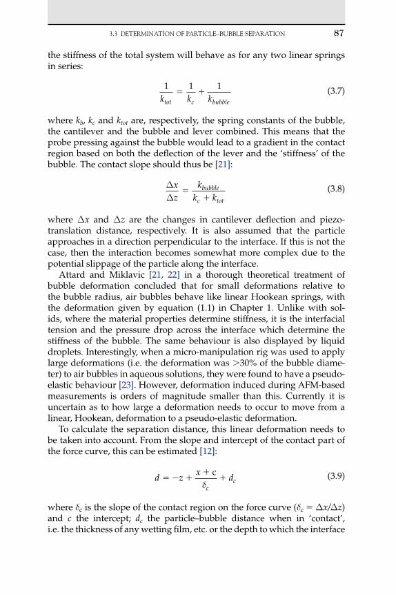
3.3 DETERMINATIONOFPARTICLE–BUBBLEsEPARATION 87
the stiffness of the total system will behave as for any two linear springs in series:
1 1 1k k ktot c bubble
(3.7)
where kb, kc and ktot are, respectively, the spring constants of the bubble, the cantilever and the bubble and lever combined. This means that the probe pressing against the bubble would lead to a gradient in the contact region based on both the deflection of the lever and the ‘stiffness’ of the bubble. The contact slope should thus be [21]:
∆∆
xz
kk k
bubble
c tot
(3.8)
where x and z are the changes in cantilever deflection and piezo-translation distance, respectively. It is also assumed that the particle approaches in a direction perpendicular to the interface. If this is not the case, then the interaction becomes somewhat more complex due to the potential slippage of the particle along the interface.
Attard and Miklavic [21, 22] in a thorough theoretical treatment of bubble deformation concluded that for small deformations relative to the bubble radius, air bubbles behave like linear Hookean springs, with the deformation given by equation (1.1) in Chapter 1. Unlike with sol-ids, where the material properties determine stiffness, it is the interfacial tension and the pressure drop across the interface which determine the stiffness of the bubble. The same behaviour is also displayed by liquid droplets. Interestingly, when a micro-manipulation rig was used to apply large deformations (i.e. the deformation was 30% of the bubble diame-ter) to air bubbles in aqueous solutions, they were found to have a pseudo-elastic behaviour [23]. However, deformation induced during AFM-based measurements is orders of magnitude smaller than this. Currently it is uncertain as to how large a deformation needs to occur to move from a linear, Hookean, deformation to a pseudo-elastic deformation.
To calculate the separation distance, this linear deformation needs to be taken into account. From the slope and intercept of the contact part of the force curve, this can be estimated [12]:
d z
xd
cc
c
(3.9)
where c is the slope of the contact region on the force curve (c x/z) and c the intercept; dc the particle–bubble distance when in ‘contact’, i.e. the thickness of any wetting film, etc. or the depth to which the interface

88 3. QUANTIFICATIONOFPARTICLE–BUBBLEINTERACTIONs
has been penetrated. This still leaves the need to either obtain the thick-ness of the wetting film from another source or assume that it is too thin to be significant, which may not be the case, particularly for very hydrophilic particles.
Perhaps the simplest method for finding the zero contact point is to use the point at which the probe snaps-in during a jump to contact as suggested by Butt [9]. In cases where there are only repulsive forces evident prior to contact, there will be no snap-in and this method cannot be used. However, in cases where estimates of particle contact angle are to be made from force curves, this approach can be very useful. An interesting approach has been described by Gillies et al. [24]. At large separations, interaction forces are very weak, and thus the bubble or droplet will behave as though it is rigid at such separations. The force versus distance data can be shifted along the distance axis to coincide with the linear Poisson–Boltzmann theory for rigid bodies. However, this technique requires determination of the surface potentials from some other source, such as by electrophoresis, making its implementation problematic in laboratories where the appropriate equip-ment is not available.
3.4 DEtErmInAtIon oF ContACt AnGLE From ForCE–DIStAnCE CurvES
As mentioned previously, the attachment of particles to air bubbles in an aqueous environment is largely mediated by the degree of hydropho-bicity of the particle. A hydrophobic particle will prefer to be in contact with the bubble, minimising its contact with surrounding water, whereas a hydrophilic particle will retain a thin wetting film. One conventional method of measuring the wettability, and hence the degree of hydropho-bicity of a surface is to measure the contact angle of a drop of water on that surface, which is the angle formed by the TPC line [25–27]. When the particle comes into contact with an air bubble, the TPC formed will likewise also contain a contact angle.
Figure 3.3 shows a basic schematic representation for the particle– bubble interaction. The particle has penetrated the bubble to a distance D. The angle represents the immersion angle of the particle, which gives an indication of the position of the TPC line with regard to the particle. The contact angle is indicated by and corresponds to the angle of con-tact internal to the droplet during conventional contact angle measure-ments. The contact angle is related to the interfacial tensions of the three interfaces present around the TPC by the Young equation:
cos
SV SL
LV (3.10)

3.4 DETERMINATIONOFCONTACTANgLEFROMFORCE–DIsTANCECURvEs 89
where indicates interfacial tension, with the subscripts SV, SL and LV denoting the solid–vapour, solid–liquid and liquid–vapour interactions, respectively.
In addition, the tension around the TPC line, called the line tension, may need to be taken into account. For macro-scale experiments, the line tension is negligible and is usually ignored, with the Young equation being a good approximation. However, at small length scales, the line tension becomes more significant and further terms need to be added. For a spherical particle in an interface, the contact angle will be [28, 29]:
cos
SL SV
LV (3.11)
where is the line tension and the geodesic curvature of the TPC line. As the TPC line is circular, then:
1
r sin (3.12)
where r is the radius of the circle drawn out by the TPC line (equal to the radius of the particle when immersed halfway).
In many systems, there exists a contact angle hysteresis between an advancing (a) and a receding contact angle (r), i.e. a different contact angle may be measured depending upon whether the TPC line is advancing or receding over a particle surface. The reason for this hysteresis is generally ascribed to roughness and heterogeneity of the surface chemistry, although other factors may be of importance, such as the existence of a contaminant layer or polymer coatings, etc. [30–35].
As the particle enters into the bubble, the TPC line is receding across the particle surface. As a result it is the receding contact angle which may be cal-culated from the approach part of the force curve, and the advancing contact
D
θα
FIGurE 3.3 A particle in direct contact with a bubble with a net force of zero, at which point it is immersed to a distance D. When no net force is present then the immersion angle is equal to the contact angle . The contact angle may be receding or advancing depend-ing upon the direction of travel of the particle.

90 3. QUANTIFICATIONOFPARTICLE–BUBBLEINTERACTIONs
angle when the particle is being extricated from the bubble. The jump- in force is dominated by capillary forces, at least in the case of a particle with a hydrophobic enough surface to be able to form a TPC line. As such, the capillary force may be related directly to r, as illustrated by equation (3.15) [36–38]:
F RCAP r 2π sin sin( ) (3.13)
where represents the interfacial tension. When the net forces are zero (i.e. FCAP 0), r will be equal to ; when this occurs, equation (1.14) may be used to calculate r [36, 39]:
cos
( )r
rR DR
(3.14)
Here the penetration depth Dr can be extracted from force curves by taking the distance from the initial jump-to-contact to the point at which the force is zero, i.e. there is no net force acting on the cantilever. This is illustrated in Figure 3.4. When the particle is withdrawn from the bubble, the TPC line is advancing across the particle, hence contact angles deter-mined are called the advancing contact angle (a). If adhesion occurs,
Da
Dr
FIGurE 3.4 A force curve, showing the relevant measurements to obtain Dr and Da. Dr is found by measuring the distance from jump-in to the point at which a net force of zero, equivalent in size to the free level force, is reached. From this distance on the approach curve, the receding contact angle r is obtained. From a similar measurement on the retract curve (Da) the advancing contact angle a may be obtained.
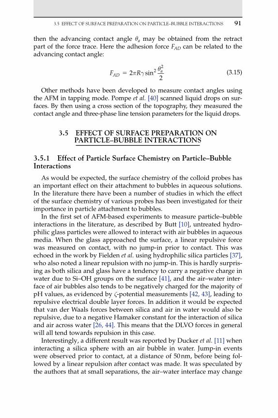
3.5 EFFECTOFsURFACEPREPARATIONONPARTICLE–BUBBLEINTERACTIONs 91
then the advancing contact angle a may be obtained from the retract part of the force trace. Here the adhesion force FAD can be related to the advancing contact angle:
F RAD
a 22
22
π
sin
(3.15)
Other methods have been developed to measure contact angles using the AFM in tapping mode. Pompe et al. [40] scanned liquid drops on sur-faces. By then using a cross section of the topography, they measured the contact angle and three-phase line tension parameters for the liquid drops.
3.5 EFFECt oF SurFACE PrEPArAtIon on PArtICLE–BuBBLE IntErACtIonS
3.5.1 Effect of Particle Surface Chemistry on Particle–Bubble Interactions
As would be expected, the surface chemistry of the colloid probes has an important effect on their attachment to bubbles in aqueous solutions. In the literature there have been a number of studies in which the effect of the surface chemistry of various probes has been investigated for their importance in particle attachment to bubbles.
In the first set of AFM-based experiments to measure particle–bubble interactions in the literature, as described by Butt [10], untreated hydro-philic glass particles were allowed to interact with air bubbles in aqueous media. When the glass approached the surface, a linear repulsive force was measured on contact, with no jump-in prior to contact. This was echoed in the work by Fielden et al. using hydrophilic silica particles [37], who also noted a linear repulsion with no jump-in. This is hardly surpris-ing as both silica and glass have a tendency to carry a negative charge in water due to Si–OH groups on the surface [41], and the air–water inter-face of air bubbles also tends to be negatively charged for the majority of pH values, as evidenced by -potential measurements [42, 43], leading to repulsive electrical double layer forces. In addition it would be expected that van der Waals forces between silica and air in water would also be repulsive, due to a negative Hamaker constant for the interaction of silica and air across water [26, 44]. This means that the DLVO forces in general will all tend towards repulsion in this case.
Interestingly, a different result was reported by Ducker et al. [11] when interacting a silica sphere with an air bubble in water. Jump-in events were observed prior to contact, at a distance of 50 nm, before being fol-lowed by a linear repulsion after contact was made. It was speculated by the authors that at small separations, the air–water interface may change

92 3. QUANTIFICATIONOFPARTICLE–BUBBLEINTERACTIONs
sign under the influence of the approaching silica particle. A similar argu-ment was used to explain the adhesion forces observed (4 mN m1), measured during retraction of the hydrophilic silica particles by Fielden et al. It has been noted elsewhere that if there is a sufficient difference in the magnitude of the surface potentials of two approaching bodies, then even if the bodies have potentials of the same sign at sufficiently small separations, an attractive force may occur [45]. It is worth bearing in mind that due to the very small surface areas of the interactions, these types of experiments are very sensitive to any contamination, even if great care is taken to prevent this. Deviations from the expected behaviour could easily be caused as a result of such contamination. In the litera-ture, papers describing colloid probe-based particle–bubble interactions describe stringent techniques to minimise the risk of contamination. The potential problems due to probe contamination are a serious concern for all SPM techniques. See Chapter 1 for more information on this subject.
Glass particles used by Butt et al. [10] were made hydrophobic by silanizing them in an atmosphere of dichloromethane. When these parti-cles were allowed to approach an air bubble, their behaviour was found to have altered from that of hydrophilic particles. This time jump-in events occurred on approach to the bubble surface with no repulsive interaction prior to contact. When the particle was retracted large adhesion occurred, with the cantilever deflecting by a greater amount than could be detected by the instrument being used [10]. In the study by Fielden et al. [37] the silica particles were hydrophobized by either reacting with octadecyltri-chlorosilane, or by dehydroxylation to create a surface with a more mod-erate degree of hydrophobicity. For the two types of hydrophobic surface, interactions between the particles and the bubbles were attractive at small separation distances. Furthermore, the attraction was dependent upon the degree of hydrophobicity of the surface. Frequently the particle was engulfed by the air bubble and much larger adhesion forces were mea-sured than with the hydrophilic particle. It was concluded that the jump-in events observed were a result of hydrophobic attraction. These two studies illustrate the importance of hydrophobicity in particle–bubble attachment and for the degree of stability of particle–bubble aggregates.
Preuss and Butt [39] measured the interactions of bubbles with silica particles coated with different surface concentrations of alkyl-thiol molecules and the resultant receding contact angles both with the col-loid probe technique and by conventional means. They noticed that as well as more hydrophilic particles having shorter jump-in distances and less adhesion than hydrophobic particles, both the r and adhe-sion forces increased as the mole fraction of alkyl-thiols was increased. As an increase in contact angle is conventionally related to an increase in hydrophobicity of a surface [27], the relationship between hydropho-bicity and the stability of particle bubble attachment is again reiterated.

3.5 EFFECTOFsURFACEPREPARATIONONPARTICLE–BUBBLEINTERACTIONs 93
In addition the authors compared the contact angles obtained from the AFM measurements with those obtained conventionally on flat surfaces. It was found that the r values obtained by the two methods differed, depending upon the contact angles measured. At low contact angles (i.e. more hydrophilic surfaces), contact angles measured with the colloid probe were higher than those measured on planar surfaces. At contact angles 60° the values obtained with the colloid probes were lower than those measured on flat surfaces, with measurements at intermediate con-tact angles in close agreement. These differences were explained by the authors as being possibly due to the differences in line tension between the different experimental set-ups [39].
The interactions of ZnS spheres with air bubbles at a range of solution pH values was examined by Gillies et al. [46, 47]. On approach, repulsion between the spheres and the bubbles was observed due to DLVO forces (the micro-spheres have a negatively charged surface in solution under the con-ditions of the experiments) and confinement of hydration layers, prior to a jump-in event. The magnitude of the repulsive force prior to jump-in was found not to vary upon alteration of solution pH to a significant effect at pH values of 8.5 or less. On increasing the pH above this level, the repulsion was increased by an order of magnitude, due to a much greater concentra-tion of negative charges on the micro-sphere surface. Contact angles mea-sured at the same time appeared to alter, based upon the number of times the micro-sphere had previously interacted with the bubble surface, leading to speculation that the ZnS surface was changing, either by being cleaned or coated by the interaction. In addition a slight increase in the receding contact angle was observed concomitant with a rise in pH. Leaving the micro-spheres in zinc solutions for extended periods of time caused the particle surface to change from a predominantly zinc hydroxide to a pre-dominantly zinc oxide surface, resulting in a greater degree of hydropho-bicity. This resulted in contact angles measured in these aged micro-spheres which were approximately 10° greater than those of the none-aged spheres.
Wangsa-Wirawan et al. [13] measured the adhesion forces due to the interactions between protein inclusion bodies and air bubbles. Both pH and ionic strength of the surrounding solution was altered and the effects measured. A maxima in the adhesion forces was reached at pH 5, with a decrease at higher pH values, although adhesion was still observed. The inclusion bodies were expected to carry a net overall negative charge at pH values 5, leading to electrostatic repulsion between the bodies and the negatively charged air–water interface. It was concluded that whilst the electrostatic forces modulated the adhesion, hydrophobic interactions between the inclusion bodies and the air–bubble played a more dominant role in the adhesion. Additionally it was reported that the ionic strength had an effect on the measured adhesion values in a way that could not be explained purely by DLVO interactions.

94 3. QUANTIFICATIONOFPARTICLE–BUBBLEINTERACTIONs
3.5.2 Effect of Surfactant on Particle–Bubble Interactions
During the froth flotation process, surfactant compounds are com-monly added to the flotation chamber to modify bubble–particle attachment and increase mineral recovery. A number of AFM-based measurements have been carried out to assess the effect of surfactants in solution on particle–bubble interactions and hence, presumably, on flota-tion efficiency.
Preuss and Butt [36, 48] studied the effects of adding two surfactants, sodium dodecyl sulphate (SDS) and dodecyltrimethylammonium bro-mide (DTAB), to solution when carrying out measurements between both hydrophobic and hydrophilic particles with air bubbles. When hydrophilic silica particles were allowed to approach the bubble in aque-ous solution without surfactant present, repulsive forces were measured prior to contact, as reported previously for hydrophilic silica particles [37, 39]. As the concentration of SDS in solution was increased, this repulsive force also increased and the decay length became decreased. As SDS has a negative charge in solution, as do the silica–water and air–water inter-faces, the most likely explanation was that the repulsion was electrostatic in origin and increased with increasing quantities of SDS at the interfaces. When the effects of DTAB were investigated long-range forces between the particles and the bubbles occurred, and adhesion was observed when retracting the particle, most probably due to DTAB coating the silica sur-face and increasing its hydrophobicity.
When silanized hydrophobic silica particles were used, capillary forces were dominant, with large adhesions on the order of 70 mN m1 detected upon particle retraction [36, 48]. In the absence of SDS, small repulsive forces were measured on approach, probably due to electrostatic repul-sion. When SDS was introduced, adhesion appeared to be dependent upon the maximum force used to press the particle into the bubble, reach-ing a threshold value of approximately 6 mN m1 for an SDS concentra-tion of 5.6 mM. Below this threshold value no adhesion was seen, with no hysteresis between the approach and the retract parts of the force curves, suggesting that the SDS was reducing the interaction between the parti-cle and the bubble. As the loading force increased above the threshold, a jump-in event occurred and high adhesion was observed. This threshold force was increased, as the SDS concentration was increased as illustrated in Figure 3.5. When the effects of DTAB were investigated, they were found to follow a similar trend to that seen with SDS. At concentrations 6 or 12 mM, for SDS or DTAB, respectively, formation of the TPC was no longer observed for the load forces that were reached [36, 48]. The most likely explanation for this behaviour is that a surfactant film was built up between particle and bubble, preventing TPC formation. As the surfactant concentration was increased, this film would most likely be thicker and

3.5 EFFECTOFsURFACEPREPARATIONONPARTICLE–BUBBLEINTERACTIONs 95
more stable. To make a TPC contact, the loading force would have to be sufficient to cause penetration of the surfactant film, characterised by the threshold force, which would increase with thicker surfactant films.
Recently, force interaction measurements have been carried out between silica glass spheres and colloidal gas aphrons (CGAs) [49]. CGAs are a form of very small (100 m) surfactant-stabilized bubbles created by high shear rate flows, first described by Sebba in 1971 as micro-foams [50]. The use of aphrons has been proposed for a number of potentially useful applications. These include the flotation of fine mineral particles [51, 52], the treatment of particulates and contaminant chemicals including solvents and heavy metals from wastewater [53–56], treatment of soil contamination [53, 57, 58], the harvesting of microbial cells [59] and extraction of protein products [58, 60, 61], and the produc-tion of tissue engineering scaffolds [62]. Sebba proposed a multi-walled structure for CGAs consisting of an outer surfactant bilayer, followed by an internal layer of surfactant solution, in turn separated by a surfactant monolayer from a central gas core. Although this putative structure has not been confirmed conclusively, there are a number of indirect experi-mental observations which suggest that the internal structure of CGAs are different from those observed with conventional foams, including x-ray diffraction, and transmission electron microscopy (TEM) [58, 63].
0 2 4
Surf.conc./mM
6 8 10 12
DTAB
SDSF
thr/R
/mN
/m
8
6
4
2
0
FIGurE 3.5 Effect of SDS and DTAB concentration on the (normalised) threshold force (F/R) needed to achieve a TPC with an air bubble in aqueous solution. Reprinted with per-mission from [36]. Copyright 1998 American Chemical Society.

96 3. QUANTIFICATIONOFPARTICLE–BUBBLEINTERACTIONs
Aphrons created in surfactant solutions which were either anionic sodium dodecyl sulfate (SDS) or cationic dodecyl trimethylammo-nium bromide (DTAB) by mixing at high sheer rates (with rotor speeds 5000 rpm) were immobilised on hydrophobic HOPG and rinsed with an excess of high purity de-ionised water [49] to remove excess surfac-tant from solution. Aphrons were made in solutions with surfactant concentrations of 1 and 2 g l1 for SDS and DTAB, respectively. Colloid probes consisting of glass spheres were then allowed to approach the surface of the aphrons (estimated bubble diameters were 50 m) and the resultant interaction forces were measured. Figure 3.6 shows exam-ple force measurements obtained when approaching aphrons produced
z-Displacement (nm)–1
–0.8
–0.6
–0.4
–0.2
0
0.2
0.4
0.6
0.8
1
–150 –100 –50 0 50 100 150 200 250 300
–1
–0.8
–0.6
–0.4
–0.2
0
0.2
0.4
0.6
0.8
1
–150 –100 –50 0 50 100 150 200 250 300
z-Displacement (nm)
A
B
For
ce, F
/R (
mN
/m)
For
ce, F
/R (
mN
/m)
FIGurE 3.6 Normalised force versus z-displacement curves obtained between aphrons created using SDS (A) and DTAB (B) in water. Each force curve is an average of several force–distance cycles (SDS 10; DTAB 9). In both cases a jump-in event is observed. However, when the glass sphere approaches the anionic SDS-stabilised aphron, a repulsive force is observed prior to contact, most likely due to repulsive (negative) charge interac-tions. When an identical glass probe approaches DTAB-stabilised aphrons, only attractive forces are seen prior to jump-in.

3.6 EFFECTOFLOADINgFORCEONPARTICLE–BUBBLEINTERACTIONs 97
using SDS and DTAB. In both cases probes became attached to the CGA surfaces. However, when approaching SDS CGAs, a repulsive force was observed prior to contact. This force was not observed with the DTAB aphrons. The difference is most likely due to charge repulsion effects, which is due to the interaction between the negatively charged glass sur-face and the negatively charged SDS. In the case of DTAB, which contains a positive charge in solution, only attractive forces are observed prior to contact. When silica was allowed to interact with CGAs in bulk flota-tion experiments, the silica was found to separate with the CGA fraction when using DTAB to create the CGAs, but a much smaller fraction was recovered when using SDS. The attachment of silica to CGAs in solution was modulated by the charge interactions between silica and the CGAs in solution, with repulsive charges preventing the attachment of the par-ticles to SDS CGAs in solution.
3.6 EFFECt oF LoADInG ForCE on PArtICLE–BuBBLE IntErACtIonS
As has been seen above in the work by Preuss and Butt, in the presence of surfactants [36, 39, 48], sometimes a threshold force is required to form a TPC contact, but there are likely to be other effects of the loading force on particle–bubble interactions. As the loading force is increased, deformation of the bubble would be expected to increase, particularly if the TPC line does not move over the particle surface. For other deformable surfaces, such as soft polymer interfaces, the maximum loading force reached has been observed to have a positive effect on the adhesion force [64]. This is not surprising, as the area of contact between the probe and the surface will increase as the surface becomes increasingly deformed. At small load-ing forces, where the force F Rp<< 2π , a deformable surface will change its shape to accommodate the particle that is being forced against it [65], thus wrapping around it, which will increase the surface area of contact.
For measurements taken between a hydrophobic silica sphere and an air bubble in concentrations of DTAB 6 mM, adhesion forces measured on retraction were observed to increase monotonically with the maxi-mum loading force which had been reached [36].
In addition Fielden et al. [37] observed that adhesion was dependent upon the loading force. As the maximum load was increased, there was a positive linear relationship with adhesion for air–silica interactions in aqueous solution. As the electrolyte concentration increased, the gradient of the slope of adhesion versus load also increased. As a TPC was formed in these measurements, it was suggested by the authors that the loading force was affecting the contact angle of the TPC.

98 3. QUANTIFICATIONOFPARTICLE–BUBBLEINTERACTIONs
3.7 EFFECt oF HyDroDynAmICS on PArtICLE–BuBBLE IntErACtIonS
As all of the particle–bubble interaction measurements carried out using an AFM-based system are undertaken in a liquid environment, it is necessary to consider the implications of hydrodynamic forces on the interactions being measured. During the process of froth flotation, the particles and bubbles are circulated around the flotation chamber at some speed, and to relate what happens in this industrial process to what hap-pens in AFM experiments, some measure of the effects of the speed of interaction between particles and bubbles necessarily has to be made. Nguyen and Evans [66] considered the hydrodynamic force acting on a sphere approaching a bubble in fluid. The hydrodynamic drag force Fh on the particle follows the following relationship, dependent upon the separation distance d from the bubble surface:
F RVfh 6 1π (3.16)
where is the dynamic viscosity of the surrounding fluid, V the velocity with which the particle approaches the bubble surface (not to be confused with the AFM piezo-drive speed), and f1 a correction factor which accounts for the deviation of the drag force from Stokes law. It is within this correction factor that the term for the separation distance appears and was derived by Nguyen and Evans to be approximated by:
f
Rd1
0 7191
0 7191
4
. .
(3.17)
Deformation of the bubble as the approaching particle encounters the thin wetting film around the bubble will lead to a reduction of V at small separation distances [20] relative to the driving speed.
Nguyen et al. [12] studied the effect of the approach speed upon the forces obtained when a spherical glass particle approached an air bubble surface. In Figure 3.7 the effect on the measured force of different piezo-translation speeds is demonstrated. As the approach speed was increased, the repulsive particle–bubble forces at short separation distances were also increased. This was possibly due to limitations on the ability of the thin water film between particle and bubble to drain in the shorter time frames imposed by the higher approach velocities. This demon-strates that hydrodynamic forces were acting as an additional repulsive force. At low piezo-approach speeds of 0.6 m s1 the hydrodynamic forces were negligible and instead surface forces were dominant. This effect has

3.7 EFFECTOFHyDRODyNAMICsONPARTICLE–BUBBLEINTERACTIONs 99
also been characterised using the colloid probe technique for a sphere approaching a solid confining wall in a fluid environment [67–71]. Due to the change in deflection of the cantilever as a result of the action of forces upon it, the actual velocity experienced by the particle differs from that applied by the piezo. A plot of the actual velocity against measured force and calculated hydrodynamic force as determined by Nguyen et al. [12] is presented in Figure 3.8. As can be seen the velocity actually decreases as the particle–bubble separation distance is decreased due to the increase in repulsive force, causing the cantilever to become deflected upwards, away from the bubble surface. A similar effect was observed by Aston and Berg [72] when approaching a droplet of n-hexadecane with a glass sphere in an SDS solution. It was found that the oil–water interface became dimpled on approach, with the distance at which this occurred increasing with increas-ing approach speed.
Another study by Nguyen et al. [38] examined the effect of the speed of approach of spherical polyethylene particles on the receding contact angles measured, obtained from force curves as described earlier. It was found that at relatively high approach speeds of 10 m s1, there was a strong influence of the approach speed on measured contact angle. At speeds below this there was little influence on contact angle. It was surmised by the authors that at the lower speeds, the measurements represented a ‘static’ contact angle.
00
2
4
6
AF
M M
easu
red
inte
ract
ion
forc
e, F
(nN
)
100 200 300
0.6
Approach speeds (µm/s)
3.05.912.217.827.939.165.497.8
400 500 600
Separation distance, D (nm)
FIGurE 3.7 Effect of the speed of approach between a particle and bubble on the meas-ured forces. Reprinted from [12]. Copyright 2004, with permission from Elsevier.

100 3. QUANTIFICATIONOFPARTICLE–BUBBLEINTERACTIONs
3.8 ConCLuSIonS
The AFM-based colloid probe technique has been used to investigate the interactions between single particles and air bubbles in aqueous solution with the aim of increasing the basic understanding of processes dependent upon this type of interaction. The effect of such particle properties as the degree of hydrophobicity has been examined in relation to properties such as particle–bubble adhesion, the favourability of long-range interaction forces to particle–bubble attachment, as well as measured contact angles in a number of studies. Measurements have also begun to characterise the effect of force and approach speed on these interactions. As froth flo-tation is a dynamic process, an understanding of the forces and kinetics involved in particle–bubble attachment may be necessary to marry AFM-based measurements to what is happening in the flotation chamber or other related industrial processes. The body of literature which now exists is not yet complete enough to give a full insight into how particle–bubble interactions on the single interaction level mediate the bulk process of froth flotation. In addition, measurements so far utilise micro-spheres with an idealised geometry. Particles used in mineral separation are more likely to be rough and irregular and quite likely more heterogeneous, leading to more complexity in their attachment to bubbles. In the industrial processes, there are a large number of different surfactants and other chemicals used to modulate mineral separation, depending upon the properties of the minerals of interest. In the AFM-based literature, only a small number of commonly available surfactants have been used. On the whole, the use of
1
0.8
0.6
0.4
0.2
00 200 400 600 800 1000
Nor
mal
ised
forc
e, F
/R (
mN
/m)
Rel
ativ
e ve
loci
ty, U
(µm
/s)
Separation distance, D (nm)
Force
Velocity
50
40
30
20
10
0
FIGurE 3.8 The relative velocity V and the measured (points) and hydrodynamic forces (line), for a piezo-movement speed of 48.8 m s1. Reprinted from [12], Copyright 2004, with permission from Elsevier.
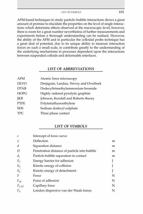
LIsTOFsyMBOLs 101
AFM-based techniques to study particle–bubble interactions shows a great amount of promise to elucidate the properties on the level of single interac-tions which determine effects observed at the macroscopic level; however, there is room for a great number nevertheless of further measurements and experiments before a thorough understanding can be realised. However, the ability of the AFM and in particular the colloidal probe technique has a great deal of potential, due to its unique ability to measure interaction forces on such a small scale, to contribute greatly to the understanding of the underlying mechanisms in processes dependent upon the interactions between suspended colloids and deformable interfaces.
LISt oF ABBrEvIAtIonS
AFM Atomic force microscopyDLVO Derjaguin, Landau, Vervey and OverbeekDTAB Dodecyltrimethylammonium bromideHOPG Highly ordered pyrolytic graphiteJKR Johnson, Kendall and Roberts theoryPTFE PolytetrafluoroethyleneSDS Sodium dodecyl sulphateTPC Three phase contact
LISt oF SymBoLS
c Intercept of force curvex Deflection md Separation distance mD Penetration distance of particle into bubble mdc Particle bubble separation in contact mE1 Energy barrier for adhesion JEk Kinetic energy of collision JEk
’ Kinetic energy of detachment JF Force NFad Force of adhesion NFCAP Capillary force NFd London dispersive van der Waals forces N
102 3. QUANTIFICATIONOFPARTICLE–BUBBLEINTERACTIONs
Fe Electrical double layer forces NFh Hydrophobic force Nk Spring constant N m1
kb Boltzmann’s constant (1.38 1023) J K1
kbubble Bubble spring constant N m1
kc Cantilever spring constant N m1
km Uncorrected measured spring constant N m1
kref Reference cantilever spring constant N m1
ktot Total spring constant of system N m1
Pa Probability of adhesionPc Probability of collisionPd Probability of detachmentr Radius of TPC circle mR Radius of sphere mV Velocity of particle m s1
W Interaction energy J m2
Wa Work of adhesion Jz Distance travelled by z-piezo m Immersion angle ° Interfacial tension N m1
c Slope of contact region of force curvehard Slope of contact region against hard surface nA m1
l Distance of probe from end of cantilever m Contact angle °a Advancing contact angle °r Receding contact angle ° Geodesic curvature of TPCf Density of fluid Pa s Line tension N m1
i Imaginary component of hydrodynamic function
references [1] J. Leja, Surface Chemistry of Froth Flotation, Plenum Press, New York, 1982. [2] B.A. Wills, Wills’ Mineral Processing Technology, seventh ed., Elsevier, Oxford, 2006. [3] V.I. Klassen, V.A. Mokrousov, An Introduction to the Theory of Flotation, second ed.,
Butterworth & Co, London, 1963.
REFERENCEs 103
[4] A.V. Nguyen, H. Stechemesser, Dynamics of the impact interaction between a fine solid sphere and a plane gas–liquid interface, in: D. Mobius, R. Miller (Eds.), Drops and Bubbles in Interfacial Research, Elsevier, Amsterdam, 1998, pp. 525–562.
[5] B.V. Derjaguin, S.S. Dukhin, Theory of flotation of small and medium sized particles, Prog. Surf. Sci. 43 (1-4) (1993) 241–266.
[6] R.-H. Yoon, Bubble–particle interactions in flotation, in: B.K. Parekh, J.D. Miller (Eds.), Advances in Flotation Technology, Society for Mining, Metallurgy, and Exploration, Inc, 1999, pp. 95–113.
[7] K.L. Sutherland, Physical chemistry of flotation. 11. Kinetics of the flotation process, J. Phys. Chem. 52 (1948) 394.
[8] R.-H. Yoon, L. Mao, Application of extended DLVO theory, IV, J. Colloid Interface Sci. 181 (1996) 613–626.
[9] H.-J. Butt, B. Capella, M. Kapple, Force measurements with the atomic force micro-scope: technique, interpretation and applications, Surf. Sci. Rep. 59 (2005) 1–152.
[10] H.-J. Butt, A technique for measuring the force between a colloidal particle in water and a bubble, J. Colloid Interface Sci. 166 (1994) 109–117.
[11] W.A. Ducker, Z. Xu, J.N. Israelachvili, Measurements of hydrophobic and DLVO forces in bubble–surface interactions in aqueous solutions, Langmuir 10 (1994) 3287–3289.
[12] A.V. Nguyen, G.M. Evans, J. Nalaskowski, J.D. Miller, Hydrodynamic interaction between an air bubble and a particle: atomic force microscopy measurements, Exp. Therm. Fluid Sci. 28 (2004) 387–394.
[13] N.D. Wangsa-Wirawan, A. Ikai, B.K. O’Neill, A.P.J. Middelberg, Measuring the interaction forces between protein inclusion bodies and an air bubble using an atomic force micro-scope, Biotechnol. Prog. 17 (2001) 963–969.
[14] D. Knebel, M. Sieber, H.-J. Galla, M. Amrein, Scanning force microscopy at the air–water interface of an air bubble coated with pulmonary surfactant, Biophys. J. 82 (2002) 474–480.
[15] N. Ishida, T. Inoue, M. Miyahara, K. Higashitani, Nano bubbles on a hydrophobic sur-face in water observed by tapping-mode atomic force microscopy, Langmuir 16 (2000) 6377–6380.
[16] P. Attard, Nanobubbles and the hydrophobic attraction, Adv. Colloid Interface Sci. 104 (2003) 75–91.
[17] H. Schubert, Nanobubbles, hydrophobic effect, hetrerocoagulation and hydrodynamics in flotation, Int. J. Miner. Process. 78 (2005) 11–21.
[18] X.H. Zhang, X.D. Zhang, S.T. Lou, Z.X. Zhang, J.L. Sun, J. Hu, Degassing and temper-ature effects on the formation of nanobubbles at the mica/water interface, Langmuir 20 (2004) 3813–3815.
[19] N. Ishida, K. Higashitani, Interaction forces between chemically modified hydropho-bic surfaces evaluated by AFM–the role of nanoscopic bubbles in the interactions, Miner. Eng. 19 (2006) 719–725.
[20] V.W.A. de Villenuve, D.G.A.L. Aarts, H.N.W. Lekkerkerker, Comparing the approach of a rigid sphere and a deformable droplet towards a deformable fluid surface, Colloids Surf. A Physicochem. Eng. Asp. (282–283) (2006) 61–67.
[21] P. Attard, S.J. Miklavcic, Effective spring constants of bubbles and droplets, Langmuir 17 (2001) 8217–8223.
[22] P. Attard, S.J. Miklavcic, Effective spring description of a bubble or a droplet interacting with a particle, J. Colloid Interface Sci. 247 (2002) 255–257.
[23] X. Fan, Z. Zhang, G. Li, N.A. Rowson, Attachment of solid particles to air bubbles in surfactant-free aqueous solutions, Chem. Eng. Sci. 59 (2004) 2639–2645.
[24] G. Gillies, C.A. Prestidge, P. Attard, Determination of the separation in colloid probe atomic force microscopy of deformable bodies, Langmuir 17 (2001) 7955–7956.
[25] C.J. van Oss, Interfacial forces in aqueous media, first ed., Marcel Dekker Inc, 1994. [26] J.N. Israelachvili, Intermolecular and Surface Forces, second ed., Academic Press,
San Diego, 1992.

104 3. QUANTIFICATIONOFPARTICLE–BUBBLEINTERACTIONs
[27] G.T. Barnes, I.R. Gentle, Interfacial Science, first ed., Oxford University Press, Oxford, 2005.
[28] R. Aveyard, J.H. Clint, Particle wettability and line tension, J. Chem. Soc. Farad. Trans. 92 (1) (1996) 85–89.
[29] L. Dong, D.T. Johnson, Adsorption of acicular particles at the liquid–fluid interfaces and the influence of line tension, Langmuir 21 (2005) 3838–3849.
[30] E.L. Decker, Contact line structure and dynamics on surfaces with contact angle hys-teresis, Langmuir 13 (1997) 6321–6332.
[31] L.W. Schwartz, S. Garoff, Contact angle hysteresis on heterogeneous surfaces, Langmuir 1 (1985) 219–230.
[32] J.-H. Wang, P.M. Claesson, J.L. Parker, H. Yasuda, Dynamic contact angles and contact angle hysteresis of plasma polymers, Langmuir 10 (1994) 3887–3897.
[33] S.B.G. O’Brien, The meniscus near a small sphere and its relationship to line pinning of contact lines, J. Colloid Interface Sci. 183 (1996) 51–56.
[34] B. Müller, M. Riedel, R. Michel, S.M. De Paul, R. Hofer, D. Heger, D. Grützmacher, Impact of nanoneter-scale roughness on contact angle hysteresis and globulin adsorp-tion, J. Vac. Sci. Technol. B 19 (5) (2001) 1715–1720.
[35] J.F. Oliver, C. Huh, S.G. Mason, Resistance to spreading of liquids by sharp edges, J. Colloid Interface Sci. 59 (3) (1977) 568–581.
[36] M. Preuss, H.-J. Butt, Direct measurement of particle–bubble interactions in aqueous electrolyte: dependence on surfactant, Langmuir 14 (1998) 3164–3174.
[37] M.L. Fielden, R.A. Hayes, J. Ralston, Surface and capillary forces affecting air bubble– particle interactions in aqueous electrolyte, Langmuir 12 (1996) 3721–3727.
[38] A.V. Nguyen, J. Nalaskowski, J.D. Miller, The dynamic nature of contact angles as measured by atomic force microscopy, J. Colloid Interface Sci. 262 (2003) 303–306.
[39] M. Preuss, H.-J. Butt, Measuring the contact angle of individual colloid particles, J. Colloid Interface Sci. 208 (1998) 468–477.
[40] T. Pompe, A. Fery, S. Herminghaus, Imaging liquid structures on inhomogeneous surfaces by scanning force microscopy, Langmuir 14 (10) (1998) 2585–2588.
[41] B.J. Kirby, E.F. Hasselbrink Jr., Zeta potential of microfluidic substrates: 1. Theory, exper-imental techniques, and effects on separations, Electrophoresis 25 (2004) 187–202.
[42] P. Saulnier, J. Lachaise, G. Morel, A. Graciaa, Zeta potential of air bubbles in surfactant solutions, J. Colloid Interface Sci. 182 (1996) 395–399.
[43] A. Graciaa, G. Morel, P. Saulner, J. Lachaise, R.S. Schechter, The zeta-potential of gas bubbles, J. Colloid Interface Sci. 172 (1995) 131–136.
[44] D.B. Hough, L.R. White, The calculation of Hamaker constants from Lifshitz theory with applications to wetting phenomena, Adv. Colloid Interface Sci. 14 (1980) 3–41.
[45] D.J. Bachman, S.J. Miklavcic, Deformation of fluid interfaces induced by electrical dou-ble layer forces and its effect on fluid–solid interactions, Langmuir 12 (1996) 4197–4204.
[46] G. Gillies, M. Kapple, H.-J. Butt, Surface and capillary forces encountered by zinc sulfide microspheres in aqueous electrolyte, Langmuir 21 (2005) 5882–5886.
[47] G. Gillies, K. Buscher, M. Preuss, M. Kapple, H.-J. Butt, K. Graf, Contact angles and wetting behaviour of single micron sized particles, J. Phys. Condens. Matter 17 (2005) S445–S464.
[48] M. Preuss, H.-J. Butt, Direct measurement of forces between particles and bubbles, Int. J. Miner. Process 56 (1999) 99–115.
[49] D.J. Johnson, N. Hilal, K.E. Waters, K. Hadler, J.J. Cilliers, Measurements of interactions between particles and colloidal gas aphrons using a combined microscopic strategy, Langmuir 49 (2009) 4880–4885.
[50] F. Sebba, Microfoams – an unexplained colloidal system, J. Colloid Interface Sci. 35 (4) (1971) 643–646.
[51] J.J. Cilliers, D.J. Bradshaw, The flotation of fine pyrite using colloidal gas aphrons, Miner. Eng. 9 (2) (1995) 235–241.
REFERENCEs 105
[52] E.A. Mansur, Y.D. Wang, Y.Y. Dai, Separation of fine particles by using colloidal gas aphrons, Chin. J. Chem. Eng. 12 (2) (2004) 286–289.
[53] P.G. Chaphalkar, K.T. Valsaraj, D. Roy, A study of the size distribution and stability of colloidal gas aphrons using a particle size analyzer, Separ. Sci. Technol. 28 (6) (1993) 1287–1302.
[54] P.G. Chaphalkar, K.T. Valsaraj, D. Roy, Flotation using microgas dispersions for the removal of pentachlorophenol from aqueous-solutions, Separ. Sci. Technol. 29 (7) (1994) 907–921.
[55] S. Ciriello, S.M. Barnett, F.J. Deluise, Removal of heavy metals from aqueous solutions using microgas dispersions, Separ. Sci. Technol. 17 (4) (1982) 521–534.
[56] D. Roy, K.T. Valsaraj, S.A. Kottai, Separation of organic dyes from wastewater by using colloidal gas aphrons, Separ. Sci. Technol. 27 (5) (1992) 573–588.
[57] D. Roy, K.T. Valsaraj, A. Tamayo, Comparison of soil washing using conventional sur-factant solutions and colloidal gas aphrons, Separ. Sci. Technol. 27 (12) (1992) 1555–1568.
[58] P. Jauregi, J. Varley, Colloidal gas aphrons: potential applications in biotechnology, TIBTECH 17 (1999) 389–395.
[59] S.V. Save, V.G. Pangarkar, Harvesting of Saccharomyces cerevisiae using colloidal gas aphrons, J. Chem Technol. Biotechnol. 62 (2) (1995) 192–199.
[60] E. Fuda, D. Bhatia, D.L. Pyle, P. Jauregi, Selective separation of beta-lactoglobulin from sweet whey using CGAs generated from the cationic surfactant CTAB, Biotechnol. Bioeng. 90 (5) (2005) 532–542.
[61] S.V. Save, V.G. Pangarkar, S.V. Kumar, Intensification of mass-transfer in aqueous 2-phase systems, Biotechnol. Bioeng. 41 (1) (1993) 72–78.
[62] E. Donaldson, J. Cuy, P. Nair, B. Ratner, Poly(vinyl alcohol)-amino acid hydrogels fabricated into tissue engineering scaffolds by colloidal gas aphron technology, Macromol. Symp. 227 (2005) 115–122.
[63] P. Jauregi, G.R. Mitchell, J. Varley, Colloidal gas aphrons (CGA): dispersion and struc-tural features, AICHE J. 46 (1) (2000) 24–36.
[64] L.-C. Xu, V. Vadillo-Rodriguez, B.E. Logan, Residence time, loading force, pH, and ionic strength affect adhesion forces between colloids and biopolymer coated surfaces, Langmuir 21 (2005) 7491–7500.
[65] D. Filip, V.I. Uricanu, M.H.G. Duits, W.G.M. Agterof, J. Mellema, Influence of bulk elasticity and interfacial tension on the deformation of gelled water-in-oil emulsion droplets: an AFM study, Langmuir 21 (2005) 115–126.
[66] A.V. Nguyen, G.M. Evans, Axisymmetric approach of a solid sphere toward a non-deformable planar slip interface in the normal stagnation flow – development of global rational approximations for resistance coefficients, Int. J. Multiphas. Flow 28 (2002) 1369–1380.
[67] F. Benmouna, D. Johanssman, Hydrodynamic interaction of AFM cantilevers with solid walls: an investigation based on AFM noise analysis, Eur. Phys. J. E 9 (5) (2002) 435–441.
[68] F. Benmouna, D. Johanssman, Hydrodynamics of particle–wall interaction in colloidal probe experiments: comparison of vertical and lateral motion, J. Phys. Condens. Matter 15 (19) (2003) 3003–3012.
[69] C.D.F. Honig, W.A. Ducker, No-slip hydrodynamic boundary condition for hydrophilic particles, Phys. Rev. Lett. 98 (2) (2007) 028305.
[70] O.I. Vinogradova, H.-J. Butt, G.E. Yakubov, F. Feuillebois, Dynamic effects on force measurements. Viscous drag on the atomic force microscope cantilever, Rev. Sci. Instrum. 72 (2001) 2330–2339.
[71] O.I. Vinogradova, G.E. Yakubov, Dynamic effects on force measurements. 2. Lubrication and the atomic force microscope, Langmuir 19 (2003) 1227–1234.
[72] D.E. Aston, J.C. Berg, Thin-film hydrodynamics in fluid interface-atomic force micros-copy, Ind. Eng. Chem. Res. 41 (2002) 389–396.

Atomic Force Microscopy in Process Engineering ©2009,ElsevierLtd107
O U T L I N E
4.1 Introduction 108
4.2 The Range of Possibilities for Investigating Membranes 109
4.3 Correspondence between Surface Pore Dimensions from AFM and MWCO 113
4.4 Imaging in Liquid and the Determination of Surface Electrical Properties 116
4.5 Effects of Surface Roughness on Interactions with Particles 120
4.6 ‘Visualisation’ of the Rejection of a Colloid by a Membrane Pore and Critical Flux 123
4.7 The Use of AFM in Membrane Development 124
4.8 Characterisation of Metal Surfaces 1264.8.1 Effect of Electropolishing of Steel Surfaces 1304.8.2 Corrosion of Metal Surfaces 1324.8.3 Biofilms at Metal Surfaces 135
4.9 Conclusions 135
Acknowledgements 136
List of Abbreviations 136References 136
InvestigatingMembranesandMembraneProcesseswithAtomicForceMicroscopy
W. Richard Bowen and Nidal Hilal
4C H A P T E R

108 4. INvEsTIgATINgMEMbRANEsANdMEMbRANEPROCEssEs
4.1 InTRODUCTIOn
Membrane processes are one of the most significant developments in process engineering in recent times. The worldwide annual sales of mem-branes and membrane equipment are now worth in excess of 1 billion Euros. Membranes find widespread application in fields as diverse as water treatment, pharmaceutical processing, food processing, biotechnology, sensors and batteries. Membranes are most usually thin polymeric sheets, having pores in the range from the micrometre to sub-nanometre, that act as advanced filtration materials. This chapter is particularly concerned with pressure-driven membrane processes – microfiltration, ultrafiltration, nanofiltration and reverse osmosis. These are usually classified according to the size of materials that they separate, with ranges typically given as 10.0 0.1 m for microfiltration (MF), 0.1–5 nm for ultrafiltration, 1 nm for nanofiltration (NF) and 1 nm for reverse osmosis (RO).
The human imagination, including the scientific imagination, is highly visual. We are most easily convinced of the existence of phenomena and processes in the physical world if we can see them. The importance of see-ing is deeply imbedded in language. Thus, when we finally understand some highly complex and abstract explanation, we may comment, ‘I see that now’. However, the size range of objects that the unaided human eye can directly observe is limited. We can use optical microscopes to extend the lower limit of this range down to objects of sizes comparable to the wavelength of light. Beyond this limit, we need to use other means to ‘see’.
Atomic force microscopy (AFM) is one means of imaging objects of dimensions from about the wavelength of light to those below a nanome-tre. Thus, in the case of membranes, it is possible to visualise the mem-brane surface properties, such as pores and morphology, using AFM. Fortuitously, the size range of objects that may be visualised by AFM cor-responds closely to the size range of surface features that determine the separation characteristics of membranes.
However, the separation characteristics of membrane interfaces do not depend solely on the physical form of surface features. In liquids, surface electrical properties and the adhesion of solutes to membrane surfaces may also have profound effects on separation performance. It is thus exceedingly fortunate that an Atomic Force Microscope may also be used to determine both of these additional controlling factors. Finally, means may be devised to quantify all of these controlling factors in liquid envi-ronments that match those of process streams.
The first intention of this chapter is to provide a concise review of the potential of AFM for the investigation of membranes and membrane processes, using examples from our own studies. The chapter will begin with illustrative examples that outline the range of possibilities of AFM
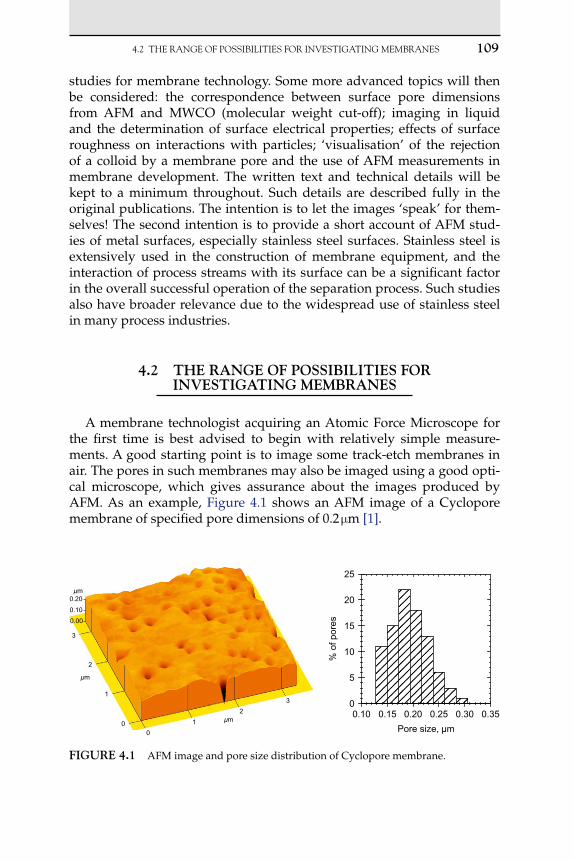
4.2 THERANgEOFPOssIbILITIEsFORINvEsTIgATINgMEMbRANEs 109
studies for membrane technology. Some more advanced topics will then be considered: the correspondence between surface pore dimensions from AFM and MWCO (molecular weight cut-off); imaging in liquid and the determination of surface electrical properties; effects of surface roughness on interactions with particles; ‘visualisation’ of the rejection of a colloid by a membrane pore and the use of AFM measurements in membrane development. The written text and technical details will be kept to a minimum throughout. Such details are described fully in the original publications. The intention is to let the images ‘speak’ for them-selves! The second intention is to provide a short account of AFM stud-ies of metal surfaces, especially stainless steel surfaces. Stainless steel is extensively used in the construction of membrane equipment, and the interaction of process streams with its surface can be a significant factor in the overall successful operation of the separation process. Such studies also have broader relevance due to the widespread use of stainless steel in many process industries.
4.2 ThE RAngE OF POSSIbILITIES FOR InVESTIgATIng MEMbRAnES
A membrane technologist acquiring an Atomic Force Microscope for the first time is best advised to begin with relatively simple measure-ments. A good starting point is to image some track-etch membranes in air. The pores in such membranes may also be imaged using a good opti-cal microscope, which gives assurance about the images produced by AFM. As an example, Figure 4.1 shows an AFM image of a Cyclopore membrane of specified pore dimensions of 0.2 m [1].
Pore size, µm
0.10 0.15 0.20 0.25 0.30 0.35
% o
f por
es
0
5
10
15
20
25
2
3
1
00
1
2
3
0.00
0.10
0.20
µm
µm
µm
FIgURE 4.1 AFM image and pore size distribution of Cyclopore membrane.

110 4. INvEsTIgATINgMEMbRANEsANdMEMbRANEPROCEssEs
Shown alongside the membrane image is the derived pore size dis-tribution. Such distributions may be readily obtained using commercial image analysis software, either automatically or manually.
Once successful images of microfiltration membranes have been obtained, it is a challenge to move downwards in expected pore size or MWCO. Thus, Figure 4.2 shows a single pore in a PCI Membranes ES625 ultrafiltration membrane, which has a specified MWCO of 25 000 [2].
The derived pore size distribution indicates a mean pore size of 5.1 nm with a standard deviation of 1.1 nm. This is a pore of dimensions suitable for separating a protein molecule. It should be noted that it is not always possible to image such small pores. In particular, it is necessary for the membrane surface roughness to have characteristic dimensions less than the pore dimensions for successful imaging.
An important challenge in science is ‘to boldly go’ where no man (or woman) has been before. Thus, Figure 4.3 shows an image and the
Pore size, nm
2 3 4 5 6 7 8 9
% o
f por
es
0
10
20
30
120.080.0
Å
Å
Å
40.00
0
40.0
80.0
120.0
0.00
1.00
2.00
FIgURE 4.2 Single pore and pore size distribution of ES625 ultrafiltration membrane.
Pore size, nm0.0 0.5 1.0 1.5 2.0
% o
f po
res
0
5
10
1612
84
00
8
4
12
16
0.001.002.00
Å
15
20
25
30
35
40
Å
Å
FIgURE 4.3 Single pore and pore size distribution of XP117 nanofiltration membrane.

4.2 THERANgEOFPOssIbILITIEsFORINvEsTIgATINgMEMbRANEs 111
corresponding pore size distribution of a single pore in a nanofiltration membrane, XP117 from PCI Membranes.
Caution is needed here. It is only in exceptional instances that it is pos-sible to obtain images of such small pores. Further, some scepticism is in order. The existence of pores in microfiltration membranes may be con-firmed by optical images. It does not seem unreasonable to push the limit of belief in pores down to the ultrafiltration range. But in the nanofiltration range, we need to be especially aware of the possibility of artefacts that look like pores and of seeing what we wish to visualise.
It was mentioned in Section 4.1 that an Atomic Force Microscope can also quantify the other key properties controlling the membrane perfor-mance. The crucial innovation in the determination of such properties is the development of colloid probes. Such probes are formed by attaching particles of dimensions of the order of 1 m to the end of tipless cantile-vers. Such attachment may be carried out using the manipulation proper-ties of an Atomic Force Microscope, but greater success is achieved with the use of specially designed micromanipulation equipment. An example of a colloid probe is shown in the electron microscopy image of Figure 4.4. The silica colloid probe shown is at about the lower size limit for success-ful micromanipulation and subsequent measurement.
If such probes are manipulated to approach a single point on a mem-brane surface in a controlled manner in an electrolyte solution, it is possible to directly quantify the electrical double layer interactions between probe and membrane, also shown in Figure 4.4, for two solutions of differing ionic strengths. Such electrical interactions are very important in determining the rejection of colloids and biological macromolecules during ultrafiltration.
The adhesion of process stream components to membranes also has an important influence on membrane performance. Ideally, such adhesion
Distance / nm
0 5 10 15 20 25 30 35 40
(F/R
) / (
mN
/m)
0
5
10
15
20
10-4 M NaCl, pH810-1 M NaCl, pH8
FIgURE 4.4 SEM image of a 0.75 m silica sphere attached to a tipless AFM cantilever and force distance curves for the approach of the probe to a Cyclopore microfiltration mem-brane in NaCl solutions at pH 8. (F is force and R is sphere radius.)

112 4. INvEsTIgATINgMEMbRANEsANdMEMbRANEPROCEssEs
should be avoided. As an example, Figure 4.5 shows a polystyrene col-loid probe and data for the retraction of such a probe after it has been pushed into contact with membrane surfaces [3].
The depths of the depressions of the curves in Figure 4.5 give direct quantification of the adhesion of the probes to the surfaces. The ES404 membrane was an existing commercial membrane and the XP117 mem-brane is a development membrane designed to have lower fouling proper-ties (both membranes are PCI Membranes). The development membrane had significantly lower adhesion and hence significantly lower fouling potential than the existing membrane.
Ultrafiltration membranes are used particularly for the processing of solutions of biological macromolecules. Such molecules are too small to immobilise singly on a cantilever. However, by adsorbing such molecules onto colloid probes, it is possible to measure their adhesion to membrane surfaces. Such a protein (BSA – bovine serum albumin)-modified probe and the corresponding adhesion data for two membranes is shown in Figure 4.6 [4].
The data shows that the protein-modified probe has significantly lower adhesion to the development membrane, XP117, than to the exist-ing commercial membrane, ES404, and hence the modified membrane has significantly lower fouling potential in the processing of such protein solutions.
Membranes are frequently used to process biological cell disper-sions. In order to elucidate such processes, it has been proved possible to immobilise single cells at tipless AFM cantilevers, creating cell probes, whilst maintaining the viability of such a cell, Figure 4.7 [5].
Such cell probes allow the direct measurement of the adhesion of bio-logical cells to membranes. Interpretation of the data for such cell probes
Piezo displacement [nm]
1000 1200 1400 1600 1800 2000
F/R
[mN
/m]
–3
–2
–1
0
1
2
3
4
5
ES 404XP 117
A
A'
B
CD
FIgURE 4.5 SEM image of a 11 m polystyrene sphere attached to a tipless AFM can-tilever and force versus piezo displacement plot (retraction) for two membranes in 102 M NaCl solution at pH 8.0 (ES404, conventional; XP117, modified).
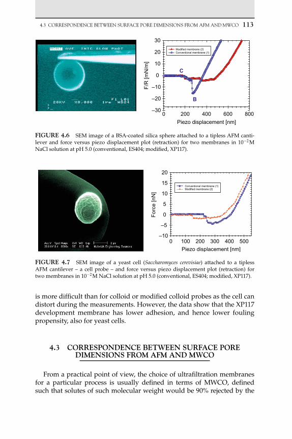
4.3 CORREsPONdENCEbETwEENsURFACEPOREdIMENsIONsFROMAFMANdMwCO 113
is more difficult than for colloid or modified colloid probes as the cell can distort during the measurements. However, the data show that the XP117 development membrane has lower adhesion, and hence lower fouling propensity, also for yeast cells.
4.3 CORRESPOnDEnCE bETWEEn SURFACE PORE DIMEnSIOnS FROM AFM AnD MWCO
From a practical point of view, the choice of ultrafiltration membranes for a particular process is usually defined in terms of MWCO, defined such that solutes of such molecular weight would be 90% rejected by the
Piezo displacement [nm]
0 200 400 600 800
F/R
[mN
/m]
–30
–20
–10
0
10
20
30
Modified membrane (2)Conventional membrane (1)
C
B
FIgURE 4.6 SEM image of a BSA-coated silica sphere attached to a tipless AFM canti-lever and force versus piezo displacement plot (retraction) for two membranes in 102 M NaCl solution at pH 5.0 (conventional, ES404; modified, XP117).
Piezo displacement [nm]
0 100 200 300 400 500
For
ce [n
N]
–10
–5
0
5
10
15
20
Conventional membrane (1)Modified membrane (2)
FIgURE 4.7 SEM image of a yeast cell (Saccharomyces cerevisiae) attached to a tipless AFM cantilever – a cell probe – and force versus piezo displacement plot (retraction) for two membranes in 102 M NaCl solution at pH 5.0 (conventional, ES404; modified, XP117).

114 4. INvEsTIgATINgMEMbRANEsANdMEMbRANEPROCEssEs
membrane. Care is required in the use of MWCO as rejection can depend on other factors such as charge and molecular shape, but it remains an extensively used parameter. It is possible to estimate the mean pore diam-eter of membranes from rejection data such as MWCO through the use of an appropriate mathematical expression. As MWCO is a historically important measure and AFM a relatively new technique, it is pertinent to investigate the correspondence between the data respectively obtained.
Such an investigation has been carried out for a series of membranes with MWCO in the range 1000–10 000 (Desal-G, Osmonics) [5]. Images of membranes obtained in air at the extremes of this range, GE (1000) and GN (10 000), are shown in Figure 4.8. The higher MWCO membrane is noticeably rougher. Indeed, there is a significant increase in surface roughness throughout the range, as shown by the data in Table 4.1.
From such images, it is possible to determine the surface pore diameter distributions of the membranes. Data is given in Table 4.2, together with the mean pore diameters from MWCO, using three differing mathematical
GE membrane
268134
03
Å
2
µm µm1
0 0
1
2
33
2
µm µm1
0 0
1
2
3
GN membrane
GE membrane GN membrane
300300
300
200200
100100
0 0
Å Å
Å Å
300
200200
100100
0 0
Å Å
3.00
2.00
1.00
0.00
2.00
1.00
0.00
FIgURE 4.8 AFM images of two Desal G membranes, GE (MWCO 1000) and GN (MWCO 10 000), at low resolution (above) and high resolution (below).
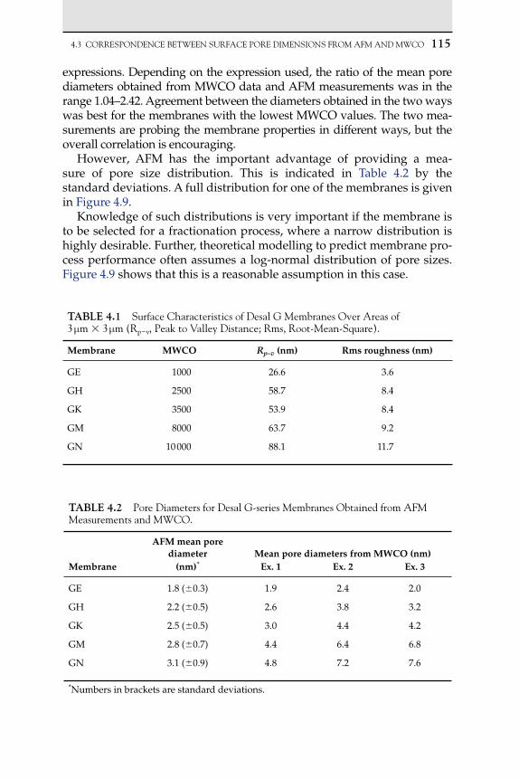
4.3 CORREsPONdENCEbETwEENsURFACEPOREdIMENsIONsFROMAFMANdMwCO 115
expressions. Depending on the expression used, the ratio of the mean pore diameters obtained from MWCO data and AFM measurements was in the range 1.04–2.42. Agreement between the diameters obtained in the two ways was best for the membranes with the lowest MWCO values. The two mea-surements are probing the membrane properties in different ways, but the overall correlation is encouraging.
However, AFM has the important advantage of providing a mea-sure of pore size distribution. This is indicated in Table 4.2 by the standard deviations. A full distribution for one of the membranes is given in Figure 4.9.
Knowledge of such distributions is very important if the membrane is to be selected for a fractionation process, where a narrow distribution is highly desirable. Further, theoretical modelling to predict membrane pro-cess performance often assumes a log-normal distribution of pore sizes. Figure 4.9 shows that this is a reasonable assumption in this case.
TAbLE 4.1 surfaceCharacteristicsofdesalgMembranesOverAreasof3m3m(Rp−v,Peaktovalleydistance;Rms,Root-Mean-square).
Membrane MWCO Rp–v (nm) Rms roughness (nm)
GE 1000 26.6 3.6
GH 2500 58.7 8.4
GK 3500 53.9 8.4
GM 8000 63.7 9.2
GN 10 000 88.1 11.7
TAbLE 4.2 Porediametersfordesalg-seriesMembranesObtainedfromAFMMeasurementsandMwCO.
AFM mean pore diameter Mean pore diameters from MWCO (nm)
Membrane (nm)* Ex. 1 Ex. 2 Ex. 3
GE 1.8 (0.3) 1.9 2.4 2.0
GH 2.2 (0.5) 2.6 3.8 3.2
GK 2.5 (0.5) 3.0 4.4 4.2
GM 2.8 (0.7) 4.4 6.4 6.8
GN 3.1 (0.9) 4.8 7.2 7.6
*Numbers in brackets are standard deviations.

116 4. INvEsTIgATINgMEMbRANEsANdMEMbRANEPROCEssEs
4.4 IMAgIng In LIqUID AnD ThE DETERMInATIOn OF SURFACE ELECTRICAL PROPERTIES
For membranes that are used in liquid systems, it is very useful to have the possibility of imaging in a solution corresponding to the pro-cessing conditions of pH and ionic content. An Atomic Force Microscope gives great control of imaging protocols, allowing investigation of the procedures that give the best membrane images, in particular the imag-ing force. Figure 4.10 shows the force of interaction between an AFM tip and a Cyclopore membrane of specified pore diameter 0.1 m in solutions at constant pH but varying ionic strength [6].
It may be seen that the range of the interaction increases greatly as the ionic strength decreases in accordance with electrical double layer theory. It is then possible to image the membrane using a force at any point on the curves in Figure 4.10. Two series of such images, one at various forces at constant ionic strength and the other at approximately constant force at vari-ous ionic strengths, are shown in Figure 4.11. It may be seen that the quality of the images improves with increasing imaging force and with increasing ionic strength. The derived pore diameter distributions also vary with the imaging conditions, as shown in the corresponding graphs in Figure 4.11 [7].
The reason for this variation may be understood from Figure 4.12, which shows calculated isopotential lines for a 101 M solution and a 104 M solution, respectively.
Pore diameter/nm
2.0 2.5 3.0 3.5 4.0 4.5 5.0
Frac
tion
of p
ores
cou
nted
0.00
0.02
0.04
0.06
0.08
0.10
0.12
0.14
0.16
Pro
babi
lity
dens
ity fu
nctio
n fR
(r)
0.00
0.02
0.04
0.06
0.08
0.10
0.12
0.14
0.16
AFM distributionTheoretical distribution
FIgURE 4.9 AFM pore size distribution for Desal GM membrane and theoretical log-normal distribution.

4.4 IMAgINgINLIqUIdANdTHEdETERMINATIONOFsURFACEELECTRICAL 117
Roughly understood, the imaging tip will follow an isopotential line during the imaging process. At the high ionic strength, all of the calcu-lated lines lie close to the membrane surface (shaded, spinning the image 360° out of the plane of the paper would generate a pore). At the lower ionic strength, some of the isopotential lines lie far from the surface, so a clear, veracious pore image would not be obtained when such a line is followed, as would be the case at low imaging forces. In conclusion, the best imaging conditions in ionic solutions are at high imaging force and, if possible and appropriate, at high ionic strength.
Though most membrane technologists now recognise the important contribution of membrane surface electrical properties in defining the separation characteristics, there remains confusion as to how best to describe and quantify such interactions. There is an unfortunate tendency in the applied membrane literature to use the terms ‘charge’ and ‘poten-tial’ loosely, almost interchangeably. There is also a regrettable lack of precision in the interpretation of membrane streaming potentials, which are the basic data most commonly used to quantify membrane surface electrical properties. The interpretation of streaming potential data can be complex even for perfectly smooth and chemically uniform planar surfaces. Most membrane surfaces have roughness comparable to electri-cal double layer dimensions, so along-the-surface-membrane streaming potential data give only some average property. Through-the-membrane streaming potential data may only be usefully interpreted in comparison
Distance (nm)
0 5 10 15 20 25 30 35
For
ce (
nN)
0
10
20
30
40
50
NaCl 10–1 MNaCl 10–2 MNaCl 10–3 MNaCl 10–4 M
FIgURE 4.10 Force versus distance curves for the approach of an AFM tip to a Cyclopore microfiltration membrane in NaCl solutions of various ionic strengths at pH 6.5.

118 4. INvEsTIgATINgMEMbRANEsANdMEMbRANEPROCEssEs
with numerical double layer calculations, as pore diameters are often less than the characteristic electrical double layer dimensions.
Fortunately, AFM, in conjunction with the colloid probe technique, offers an alternative means of membrane surface electrical properties characterisation. If a colloid probe is approached towards a surface, it is possible to quantify the force of interaction. Typical data is shown in Figure 4.13 for a Desal DK membrane, which is one of the least rough membranes [7].
IF = 4.4 nN10-1 M
Pore size, µm
A
0.05 0.10 0.15
%
0
10
20
30
40
50
2
Imaging force = 4.35 nN
NaCl 10-1
2
1
1
µm
µm00
2
1.5
1.5
Imaging force = 33 nN
NaCl 10-4
2
1
0.5
0.51
µm
µm00
2
1.5
1.5
Imaging force = 32.1 nN
NaCl 10-3
2
1
0.5
0.51
µm
µm00
2
1.5
1.5
Imaging force = 33.2 nN
NaCl 10-2
2
1
0.5
0.51
µm
µm0
0
2
Imaging force = 12.9 nN
NaCl 10-1
2
1
1
µm
µm00
2
Imaging force = 33.8 nN
NaCl 10-1
2
1
1
µm
µm00
IF = 33.0 nN10-4 M
Pore size, µm
0.05 0.10 0.15 0.20
%
0
10
20
30
40
50IF = 33.1 nN
10-3 M
Pore size, µm
0.05 0.10 0.15
%
0
10
20
30
40
50IF = 33.2 nN
10-2 M
Pore size, µm
0.05 0.10 0.15
%
0
10
20
30
40
50
IF = 12.9 nN10-1 M
Pore size, µm
B C
A B C
D E F
D E F
0.05 0.10 0.15
%
0
10
20
30
40
50IF = 33.8 nN
10-1 M
Pore size, µm
0.05 0.10 0.15
%
0
10
20
30
40
50
FIgURE 4.11 AFM images of a Cyclopore membrane in electrolyte solutions. (a)–(c) at various forces in 101 M NaCl solution; (c), (d)–(f) at approximately constant force at vari-ous ionic strengths. All data at pH 6.5 (IF-imaging force).
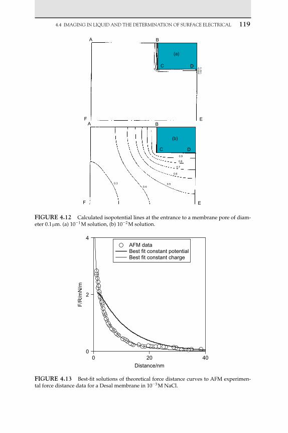
4.4 IMAgINgINLIqUIdANdTHEdETERMINATIONOFsURFACEELECTRICAL 119
A B
C D0.70.40.1
0.9
0.8
0.7
0.6
0.50.4
0.3
(a)
EF
C D
A
(b)
B
F E
FIgURE 4.12 Calculated isopotential lines at the entrance to a membrane pore of diam-eter 0.1 m. (a) 101 M solution, (b) 102 M solution.
Distance/nm
0 20 40
F/R
/mN
/m
0
2
4AFM dataBest fit constant potentialBest fit constant charge
FIgURE 4.13 Best-fit solutions of theoretical force distance curves to AFM experimen-tal force distance data for a Desal membrane in 103 M NaCl.

120 4. INvEsTIgATINgMEMbRANEsANdMEMbRANEPROCEssEs
Moreover, if the surface potential or surface charge of the colloid has been determined and the solution is of defined ionic content, it is possi-ble to calculate the potential or charge of the surface under investigation by matching the experimentally obtained curves to theoretical calcula-tions on the basis of electrical double layer theory. In the example shown, the best-fit membrane surface charge was 0.00114 C m2 and the best-fit membrane surface potential was 64 mV. Furthermore, an important advantage of the colloid probe technique is that it allows exploration of variations in surface electrical interactions at different points on the membrane surface, as the following section shows.
4.5 EFFECTS OF SURFACE ROUghnESS On InTERACTIOnS WITh PARTICLES
Surfaces are usually imaged using sharp tips in order to produce images with the highest possible definition. However, from a processing viewpoint, an important factor is how process stream components such as solutes and colloidal particles interact with the surface. If a surface has fea-ture variations that have dimensions comparable with those of the process stream components, then such interactions may show variations at differ-ent locations on the surface. An effective way of gauging such effects is to image the surface with an appropriate stream component, e.g. a particle that is immobilised to form a colloid probe. Figure 4.14 shows results for a reverse osmosis membrane (AFC99, PCI Membranes) imaged in saline solution with first a sharp tip and then a 4.2 m silica sphere [8].
P–v = 560 nmRms = 66nm
A B
µm
µmµm
0.4
0.2
0
µm
0.12
0.16
0.2
0.04
0
44
33
22
1 1
0 0
µmµm
44
33
22
1 1
0 0
P–v = 186 nmRms = 21nm
FIgURE 4.14 AFC99 membrane imaged with a tip (A) and with a 4.2 m colloid probe (B) (P–v, peak to valley; Rms, root mean square).

4.5 EFFECTsOFsURFACEROUgHNEssONINTERACTIONswITHPARTICLEs 121
The membrane surface features are still apparent but less well defined in the colloid probe image. This is a rather rough membrane showing clear peaks and valleys. Following imaging, it is possible to position the colloid probe at any point on the surface to quantify colloid–surface interactions. Figure 4.15 shows long-range electrostatic interactions quan-tified at peaks and valleys respectively, and some analysis of the data is presented in Table 4.3.
Both the magnitude and range of the electrical double layer interac-tions on the peaks are greatly reduced compared to that in the valleys. In both cases, the range is very different from that at a planar surface, both experimental – data for mica is shown for comparison – or theoretical, the Debye length. It is also possible to quantify the adhesive interaction between colloid probe and membrane surface at different locations, as shown in Figure 4.16 and Table 4.4.
AFC99, valleysAFC99, peaks
Distance/nm
0 10 20 30 40
Distance/nm
0 10 20 30 40
F/R
/mN
/m
0.1
1
10
F/R
/mN
/m
0.1
1
10
10–1 M
10–2 M10–3 M
10–1 M
10–2 M10–3 M
FIgURE 4.15 Long-range electrostatic interactions at peaks and valleys for an AFC99 membrane at various ionic strengths in NaCl solutions (F, force; R, sphere radius).
TAbLE 4.3 EffectiveExperimentaldecayLengthsforApproachCurvesbetweensilicaColloidProbeandAFC99MembraneandMica,anddebyeLength.
Effective decay lengths (nm)[NaCl] (M) Membrane peak Membrane valley Mica Debye length (nm)
103 7.71.4 12.11.5 9.20.5 9.6
102 3.20.6 6.81.2 3.50.3 3.1

122 4. INvEsTIgATINgMEMbRANEsANdMEMbRANEPROCEssEs
The adhesion of the colloid probe is markedly lower at the peaks on the membrane surface than in the valleys, with the difference increasing with decreasing salt concentration, and reaching a factor of more than 20 in 103 M solution. The wide variation in interactions shows that theoret-ical descriptions of membrane fouling need to take surface morphology into explicit account. Further, the results show that the selection of mem-branes for the filtration of specific process streams would benefit from an assessment of the size of likely foulants and the membrane roughness, especially the periodicity of the roughness. Fouling could be minimised
Separation distance / nm
0 50 100 150
F/R
/ m
N/m
–8
–6
–4
–2
0
2
4
6
PeakValley
FIgURE 4.16 Adhesion of a silica colloid probe at a peak and a valley on an AFC99 membrane in 103 M NaCl solution (pull-off force).
TAbLE 4.4 NormalisedAdhesionForcesforsilicaColloidProbesandAFC99Membrane.
Surface type [NaCl] (M) F/R (mN/m)
Membrane peak 103 0.3 (0.17)
102 1.4 (0.43)
101 2.3 (0.48)
Membrane valley 103 6.5 (2.2)
102 8.1 (3.5)
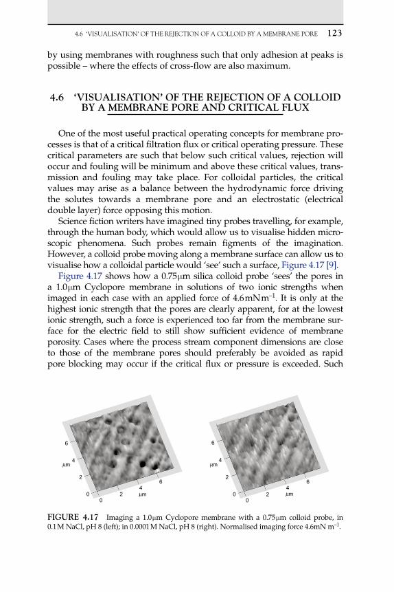
4.6 ‘vIsUALIsATION’OFTHEREjECTIONOFACOLLOIdbyAMEMbRANEPORE 123
by using membranes with roughness such that only adhesion at peaks is possible – where the effects of cross-flow are also maximum.
4.6 ‘VISUALISATIOn’ OF ThE REjECTIOn OF A COLLOID by A MEMbRAnE PORE AnD CRITICAL FLUx
One of the most useful practical operating concepts for membrane pro-cesses is that of a critical filtration flux or critical operating pressure. These critical parameters are such that below such critical values, rejection will occur and fouling will be minimum and above these critical values, trans-mission and fouling may take place. For colloidal particles, the critical values may arise as a balance between the hydrodynamic force driving the solutes towards a membrane pore and an electrostatic (electrical double layer) force opposing this motion.
Science fiction writers have imagined tiny probes travelling, for example, through the human body, which would allow us to visualise hidden micro-scopic phenomena. Such probes remain figments of the imagination. However, a colloid probe moving along a membrane surface can allow us to visualise how a colloidal particle would ‘see’ such a surface, Figure 4.17 [9].
Figure 4.17 shows how a 0.75 m silica colloid probe ‘sees’ the pores in a 1.0 m Cyclopore membrane in solutions of two ionic strengths when imaged in each case with an applied force of 4.6 mN m–1. It is only at the highest ionic strength that the pores are clearly apparent, for at the lowest ionic strength, such a force is experienced too far from the membrane sur-face for the electric field to still show sufficient evidence of membrane porosity. Cases where the process stream component dimensions are close to those of the membrane pores should preferably be avoided as rapid pore blocking may occur if the critical flux or pressure is exceeded. Such
6
4
2 2
00
24
6
6
4
00
24
6
µm
µm
µm
µm
FIgURE 4.17 Imaging a 1.0 m Cyclopore membrane with a 0.75 m colloid probe, in 0.1 M NaCl, pH 8 (left); in 0.0001 M NaCl, pH 8 (right). Normalised imaging force 4.6mN m–1.

124 4. INvEsTIgATINgMEMbRANEsANdMEMbRANEPROCEssEs
conditions may, however, be theoretically predicted. Thus, Figure 4.18 shows the time dependence of flux for such a case where the critical pressure is cal-culated to be 130 kPa. Above this pressure, there is a rapid decrease in flux with time, but below this pressure, only a very gradual flux decrease occurs.
4.7 ThE USE OF AFM In MEMbRAnE DEVELOPMEnT
The ability of AFM to guide the development of improved membranes has been shown in the development of polysulphone-sulphonated poly(ether ether) ketone (PSU/SPEEK) blend membranes. The aim of the work was to develop highly charged membranes with correspondingly low adhesion characteristics and high critical fluxes [10]. The SPEEK pro-vides negative charges, as shown by the structure in Figure 4.19.
One great benefit of SPEEK is that it acts as a pore formation–promoting agent. This gives membranes high porosity and high fluxes, as shown by the increase in water flux, with increasing SPEEK content shown in Figure 4.20.
The increase in porosity may be directly confirmed by high-resolution images of an unmodified PSU membrane and a PSU/SPEEK membrane with 5% of the charged polymer, Figure 4.21.
0 5 10 15 20 25
Flu
x / m
s–1
0.0000
0.0001
0.0002
0.0003
0.0004
0.0005
0.0006
250 kPa50 kPa
Time / min
FIgURE 4.18 Filtration fluxes as a function of time for filtration of particles very close in dimensions to the pore dimensions. Silica particles, 0.001 M NaCl, pH 6.0, mean particle diameter 86 nm, mean pore diameter 85 nm, calculated critical pressure 130 kPa.
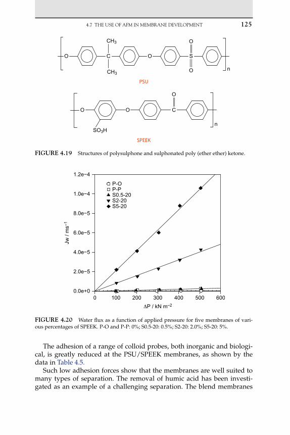
4.7 THEUsEOFAFMINMEMbRANEdEvELOPMENT 125
The adhesion of a range of colloid probes, both inorganic and biologi-cal, is greatly reduced at the PSU/SPEEK membranes, as shown by the data in Table 4.5.
Such low adhesion forces show that the membranes are well suited to many types of separation. The removal of humic acid has been investi-gated as an example of a challenging separation. The blend membranes
PSU
SPEEK
O C O S
O
O
CH3
CH3
n
O O C
O
nSO3H
FIgURE 4.19 Structures of polysulphone and sulphonated poly (ether ether) ketone.
ΔP / kN m–2
0 100 200 300 400 500 600
Jw /
ms–
1
0.0e+0
2.0e−5
4.0e−5
6.0e−5
8.0e−5
1.0e−4
1.2e−4
P-OP-PS0.5-20S2-20S5-20
FIgURE 4.20 Water flux as a function of applied pressure for five membranes of vari-ous percentages of SPEEK. P-O and P-P: 0%; S0.5-20: 0.5%; S2-20: 2.0%; S5-20: 5%.
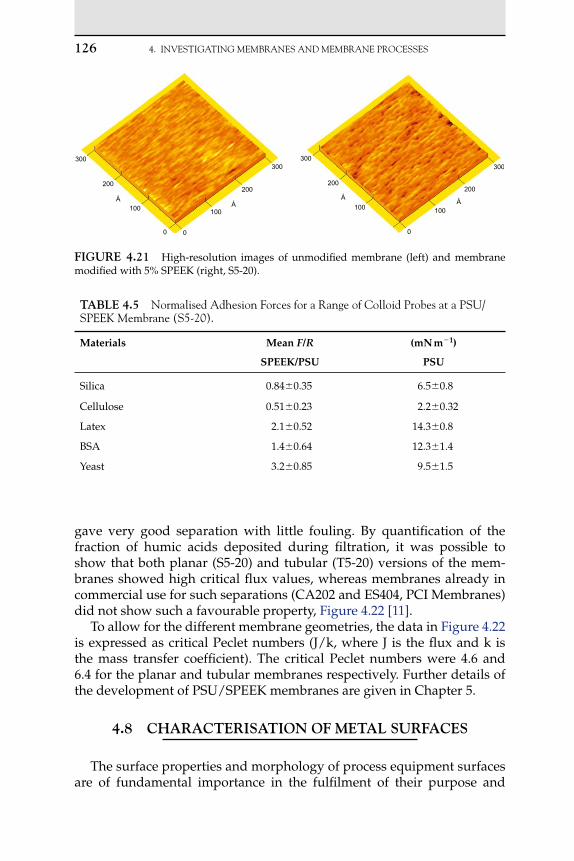
126 4. INvEsTIgATINgMEMbRANEsANdMEMbRANEPROCEssEs
gave very good separation with little fouling. By quantification of the fraction of humic acids deposited during filtration, it was possible to show that both planar (S5-20) and tubular (T5-20) versions of the mem-branes showed high critical flux values, whereas membranes already in commercial use for such separations (CA202 and ES404, PCI Membranes) did not show such a favourable property, Figure 4.22 [11].
To allow for the different membrane geometries, the data in Figure 4.22 is expressed as critical Peclet numbers (J/k, where J is the flux and k is the mass transfer coefficient). The critical Peclet numbers were 4.6 and 6.4 for the planar and tubular membranes respectively. Further details of the development of PSU/SPEEK membranes are given in Chapter 5.
4.8 ChARACTERISATIOn OF METAL SURFACES
The surface properties and morphology of process equipment surfaces are of fundamental importance in the fulfilment of their purpose and
300
200200
300300
200
100
0
100
200
300
100
0 0
100
ÅÅ
ÅÅ
FIgURE 4.21 High-resolution images of unmodified membrane (left) and membrane modified with 5% SPEEK (right, S5-20).
TAbLE 4.5 NormalisedAdhesionForcesforaRangeofColloidProbesataPsU/sPEEKMembrane(s5-20).
Materials Mean F/R (mN m1)
SPEEK/PSU PSU
Silica 0.840.35 6.50.8
Cellulose 0.510.23 2.20.32
Latex 2.10.52 14.30.8
BSA 1.40.64 12.31.4
Yeast 3.20.85 9.51.5

4.8 CHARACTERIsATIONOFMETALsURFACEs 127
applications in (bio) process industries. Many environments to which they may become exposed are potentially corrosive, and thus more corrosion-resistant surfaces may have greater operational lifetimes. In addition, surfaces may become fouled, leading to a reduction in operat-ing efficiency, especially for surfaces involved in the desalination and water treatment industries. This section will concentrate on the use of AFM to characterise the surface features and morphology of metal sur-faces of interest in process engineering applications.
One of the most commonly used materials in process equipment is stainless steel in various forms. In Figure 4.23, by way of example, are shown three 3-dimensional 50 50 m scans of different steel surfaces of difference roughness characteristics, imaged in air [12].
These are: (a) a ‘highly polished’ stainless steel surface with an opti-cally fine finish, (b) the surface of a stainless steel sample disk, such as that commonly used for affixing AFM samples and (c) a sample stub similar to that in (b), which has undergone significant pitting owing to corrosion. Surface (b) contains ridges caused by the mechanical polish-ing of the surface, which are not visible in (a). For the corroded sam-ple, there is clearly a much greater variation in the height of surface features and a greater number of asperities. This can be seen from the roughness parameters obtained from the height data contained in these
JHA / k
0 5 10 15 20 25 30
Dfr
actio
nal
0.00
0.02
0.04
0.06
0.08
0.10
0.12
0.14
0.16
0.18
CA202, ES404S5-20T5-20
FIgURE 4.22 Fractional deposition of humic acids at different operating fluxes. The intercepts on the x-axis indicate the critical fluxes.

128 4. INvEsTIgATINgMEMbRANEsANdMEMbRANEPROCEssEs
726.59 nm0 nm
50 µm
25 µm
0 µm
25 µm
50 µm
0 µm
50 µm
25 µm
25 µm
50 µm
1.78 µm
3.56 µm
0 µm0 µm
0 µm
50 µm
25 µm
25 µm
50 µm
0.73 µm1.47 µm
0 µm0 µm
0 µm
A
C
B
FIgURE 4.23 3D topographic images of surfaces with three different grades of roughness.

4.8 CHARACTERIsATIONOFMETALsURFACEs 129
images. Table 4.6 shows surface characteristics obtained from such AFM images.
The differences in the roughness average (Ra) and root mean square roughness (RMS) show that the statistical variation in height of the individual points in each image becomes greater from sample (a) to (c), whilst the average height and maximum range show that the magnitude of the variations in height, and hence size, of the surface features is much greater from sample (a) to (c).
Adhesion measurements were taken with a CaCO3 crystal, Figure 4.24, at five different points on the sample surface, with a total of approximately 100 measurements per sample, and mean adhesion values were calculated.
TAbLE 4.6 surfaceCharacteristicsObtainedfromAFMImages.
Surface Area Ra (nm) RMS (nm) Average height (nm) Maximum range (nm)
(a) 38.3 49.5 361.1 726.6
(b) 124.3 170.1 785.4 1407.5
FIgURE 4.24 SEM image of a CaCO3 crystal mounted as a probe on the apex of an AFM cantilever.

130 4. INvEsTIgATINgMEMbRANEsANdMEMbRANEPROCEssEs
Figure 4.25 shows a summary of the adhesion data measured between the probe and each of the stainless steel surfaces of interest.
As can be seen, sample (c) has the lowest adhesion value measured, with the probe detaching at a mean force of 65.5 nN. Samples (b) and (a) showed higher adhesion, with values of 99.3 and 83.2 nN, respectively. As a general rule, roughness on two interacting surfaces reduces the area of contact between these surfaces, which would be expected to lead to a decrease in the measured adhesion. This could explain the increase in adhesion seen with surfaces (b) and (a) compared with the relatively rough surface (c). However, the least rough sample (a) has a lower adhe-sion than that of sample (b). If there were a simple relationship between the roughness of the surfaces and adhesion, this would not be expected to be the case. However, the relationship between roughness and adhe-sion is not easily defined and can be dependent upon the length scales of the roughness on the individual surfaces as well as the geometry of interaction of the surfaces. In some cases, if the length scales of the probe or asperities on the probe are similar to the roughness of the surface, it could be possible for an increased contact area to be achieved [13–16].
4.8.1 Effect of Electropolishing of Steel Surfaces
Electropolishing is a process of dissolving the very top layer of a metal surface to bring about an increase in the optical brightness or reflectivity of a surface by the reduction of surface roughness. One advantage of this over polishing of surfaces by mechanical means is the absence of defects in the surfaces due to scratches. As the characterisation of the roughness
0
20
40
60
80
100
120
Polished steel Unpolished steelsample surface
Corroded steel
Mea
n ad
hesi
on (
nN)
FIgURE 4.25 Summary of measured adhesion values between a calcium carbonate col-loid probe and three steel sample surfaces.

4.8 CHARACTERIsATIONOFMETALsURFACEs 131
of surfaces at fine levels of detail is easily accomplished by AFM imag-ing, the monitoring of the polishing of surfaces is an obvious application.
Abbot and co-workers used AFM both in air and in situ in liquid to monitor the changes in morphology over time of a stainless steel sur-face during electropolishing with an ionic liquid [17]. Roughness values, described by maximum z-height, were 597 and 88 nm for the unpolished and polished surfaces respectively. As the z-max figures for the unpolished surface were likely to be greater than would be expected owing to the sur-face not being flat, the authors also calculated roughness as a percentage difference in the flat scanning area versus the actual surface area of the sample. This yielded roughness values of 7.9% for the unpolished surface and 0.2% for the polished surface. It was also noted that a trough was seen to have been etched out at the boundary between the polished and unpol-ished areas, varying in depth from 1–2 m, Figure 4.26.
C
BA
(x = 35.6µm)
y / µm
Hei
ght/n
m
500
–500
–1000
–1500
–2000
–25000.0 10.0 20.0 30.0 40.0 50.0 60.0 70.0
0
70.0
60.0
50.0
40.0
30.0
20.0
10.0
10.0 20.0 30.0 40.0 50.0 60.0
x / µm
y / µ
m
Hei
ght/n
m
10.0 20.0 30.0 40.0 50.0 60.0 70.060.0
50.040.0
30.020.0
10.0
y / µm
x / µ
m
500
–500
–1000
–1500
–2000
–2500
0
FIgURE 4.26 AFM images obtained at the transition between polished and non- polished areas of a stainless steel surface. (a) and (b) show the same areas in 2D and 3D modes. Unpolished surface is flat but has high roughness, whereas the polished surface is relatively smooth, but still shows large height variations. At the interface is an etched trench. (c) shows a line profile from the image, with the unpolished section on the left and polished on the right. Reproduced from [17].
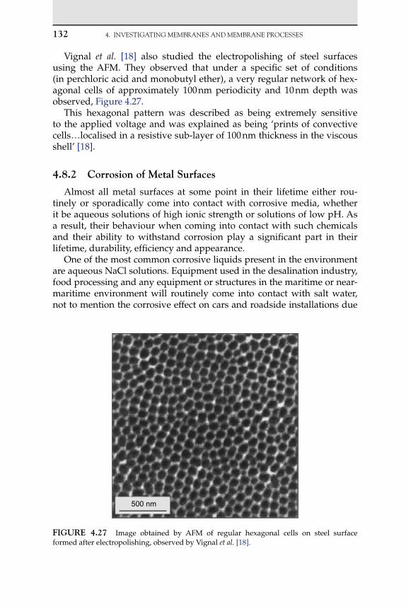
132 4. INvEsTIgATINgMEMbRANEsANdMEMbRANEPROCEssEs
Vignal et al. [18] also studied the electropolishing of steel surfaces using the AFM. They observed that under a specific set of conditions (in perchloric acid and monobutyl ether), a very regular network of hex-agonal cells of approximately 100 nm periodicity and 10 nm depth was observed, Figure 4.27.
This hexagonal pattern was described as being extremely sensitive to the applied voltage and was explained as being ‘prints of convective cells…localised in a resistive sub-layer of 100 nm thickness in the viscous shell’ [18].
4.8.2 Corrosion of Metal Surfaces
Almost all metal surfaces at some point in their lifetime either rou-tinely or sporadically come into contact with corrosive media, whether it be aqueous solutions of high ionic strength or solutions of low pH. As a result, their behaviour when coming into contact with such chemicals and their ability to withstand corrosion play a significant part in their lifetime, durability, efficiency and appearance.
One of the most common corrosive liquids present in the environment are aqueous NaCl solutions. Equipment used in the desalination industry, food processing and any equipment or structures in the maritime or near-maritime environment will routinely come into contact with salt water, not to mention the corrosive effect on cars and roadside installations due
500 nm
FIgURE 4.27 Image obtained by AFM of regular hexagonal cells on steel surface formed after electropolishing, observed by Vignal et al. [18].

4.8 CHARACTERIsATIONOFMETALsURFACEs 133
to salt spray from roads during winter. Sanchez and colleagues [19] exam-ined the early stages of corrosion of high-strength steel in dilute (50 mM) solutions of NaCl. The steels examined were of the type used for the rein-forcing of concrete structures, which are prone to corrosion when exposed to salt water due to the porous nature of the concrete and consisting of ferrite and cementite. The authors scanned the same area of the steel sur-face for over 2 h and observed changes in the surface morphology due to interaction with the corrosive media. Snapshots of the sample at different times are shown in Figure 4.28.
Initially (t 0) the polishing marks and scratches are still visible, but disappear after 50 minutes, when the surface was observed to be increas-ingly rough as the growth of oxides on the surface occurred. After approx-imately 50 min, and later, a series of ridges were observed to appear. The authors concluded that this was the lamellar structure of pearlite (the mixture of ferrite and cementite phases) appearing as the ferrite matrix was selectively attacked by the salt solution. The change in the surface roughness was monitored as a function of time, allowing the quantitative assessment of corrosion of the surface, Figure 4.29.
Z: 21.6nm
Z: 151.8nm
X: 5.0µmX: 5.0µm
X: 5.0µmX: 5.0µm
Z: 24.1nm
Z: 40.1nm
A B
C D
FIgURE 4.28 Steel surface after varying lengths of exposure to 50 mM NaCl solution. (a) 0 min; (b) 30 min; (c) 50 min; (d) 2 h 15 min. Reproduced from [19].
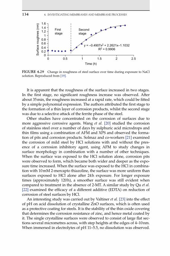
134 4. INvEsTIgATINgMEMbRANEsANdMEMbRANEPROCEssEs
It is apparent that the roughness of the surface increased in two stages. In the first stage, no significant roughness increase was observed. After about 35 min, the roughness increased at a rapid rate, which could be fitted by a simple polynomial expression. The authors attributed the first stage to the formation of a thin layer of corrosion products, whilst the second stage was due to a selective attack of the ferrite phase of the steel.
Other studies have concentrated on the corrosion of surfaces due to more aggressive corrosive agents. Wang et al. [20] studied the corrosion of stainless steel over a number of days by sulphuric acid microdrops and thin films using a combination of AFM and XPS and observed the forma-tion of pits and corrosion products. Solmaz and co-workers [21] examined the corrosion of mild steel by HCl solutions with and without the pres- ence of a corrosion inhibitory agent, using AFM to study changes in surface morphology in combination with a number of other techniques. When the surface was exposed to the HCl solution alone, corrosion pits were observed to form, which became both wider and deeper as the expo-sure time increased. When the surface was exposed to the HCl in combina-tion with 10 mM 2-mercapto thiazoline, the surface was more uniform than surfaces exposed to HCl alone after 24 h exposure. For longer exposure times (approximately 120 h), a smoother surface was still evident when compared to treatment in the absence of 2-MT. A similar study by Qu et al. [22] examined the efficacy of a different additive (EDTA) on reduction of corrosion of steel surfaces by HCl.
An interesting study was carried out by Valtiner et al. [23] into the effect of pH on acid dissolution of crystalline ZnO surfaces, which is often used as a protective coating for steels. It is the stability of the thin oxide covering that determines the corrosion resistance of zinc, and hence metal coated by it. The single crystalline surfaces were observed to consist of large flat sec-tions several micrometres across, with step heights at the edges of 4–10 nm. When immersed in electrolytes of pH 11–5.5, no dissolution was observed.
Secondstage
Firststage
1.61.41.2
10.80.60.40.2
0Sur
face
rou
ghne
s (n
m)
0 0.5 1 1.5 2
Time (h)
y = –0.4907x2 + 2.2621x–1.1032R2 = 0.9906
2.5
FIgURE 4.29 Change in roughness of steel surface over time during exposure to NaCl solution. Reproduced from [19].
4.9 CONCLUsIONs 135
At pH 5.5, dissolution began to occur, but only at the step edges, not in the centre of the crystal planes. At pH values below this, as the pH decreased the dissolution rate increased, with a significant change in behaviour occurring below pH 4.0. Below this value, dissolution also began to occur at the flat crystal surfaces, although it was still most pronounced at the edges. It was suggested that this behaviour was due to the presence of oxygen in the step edges, which would be much more prone to attack by solution protons than the flat surfaces, which are positively charged at the higher pH values.
A number of other studies have used AFM alongside other techniques to characterise a number of different coatings to protect metal surfaces from corrosion and wear, including TiN and ZrN thin films [24]; Sn–Ni and Sn–Cu alloy coatings [25, 26]; CrN films for enhanced wear resis-tance [27] and zirconia-based primers as coatings on aluminium [28].
4.8.3 biofilms at Metal Surfaces
Yu and colleagues [29] examined the difference between nano- and microcrystallization of stainless steel surfaces and the effect on the adhe-sion of biofilms. Using an AFM tip coated in a synthetic peptide to simu-late a biofilm, adhesion measurements were made against nanocrystalline and microcrystalline surfaces. It was found that the measured adhesion in air was significantly reduced for the nanocrystalline surface compared with the microscrystalline surface. These observations were matched by similar results from the observations of attachment of whole bacterial cells to the same surfaces in bulk solution.
4.9 COnCLUSIOnS
The many benefits of AFM in investigations of membranes and mem-brane processes may be summarised as:
1. Atomic force microscopy can determine the key properties of syn-thetic membranes: pore size distribution, surface morphology and surface roughness, surface electrical properties and surface adhesion.
2. Correspondence between surface pore dimensions from AFM and MWCO is good. In addition, AFM gives surface pore size distribution.
3. Operations in liquid and colloid probe techniques are particular advantages of AFM.
4. AFM can establish the effects of changes in interactions over the sur-face of membranes, e.g. due to local morphology.
5. AFM allows the visualisation of solute/membrane interactions.6. AFM is a very useful asset in assessing the properties of membranes
during their development.

136 4. INvEsTIgATINgMEMbRANEsANdMEMbRANEPROCEssEs
Indeed, it is apparent that the capabilities of AFM are very closely mat-ched to the knowledge requirements of membrane scientists and engineers.
In addition, AFM is a very useful technique for investigating the interaction of process streams with the materials of construction of pro-cess equipment, including studies of particle adhesion and the effects of corrosion.
ACknOWLEDgEMEnTS
We thank all who have contributed to this research, especially Teodora Doneva, Daniel Johnson, Bob Lovitt, Martin Peer, Peter Williams, Chris Wright and Huabing Yin.
LIST OF AbbREVIATIOnS
BSA bovine serum albuminEDTA ethylenediaminetetraacetic acidMF microfiltrationMT mercapto thiazolineMWCO molecular weight cut-offNF nanofiltrationPSU polysulphoneRO reverse osmosisSPEEK sulphonated poly (ether ether) ketoneUF ultrafiltrationXPS X-ray photoelectron spectroscopy
Names of membranes are manufacturers’ codes.
References[1] W.R. Bowen, N. Hilal, R.W. Lovitt, P.M. Williams, Atomic force microscope studies of
membranes: surface pore structures of Cyclopore and Anopore membranes, J. Memb. Sci. 110 (1996) 233–238.
[2] W.R. Bowen, N. Hilal, R.W. Lovitt, P.M. Williams, Visualisation of an ultrafiltration membrane by non-contact atomic force microscopy at single pore resolution, J. Memb. Sci. 110 (1996) 229–232.
[3] W.R. Bowen, N. Hilal, R.W. Lovitt, C.J. Wright, A new technique for membrane char-acterisation: direct measurement of the force of adhesion of a single particle using an atomic force microscope, J. Memb. Sci. 139 (1998) 269–274.

REFERENCEs 137
[4] W.R. Bowen, N. Hilal, R.W. Lovitt, C.J. Wright, Characterisation of membrane sur-faces: direct measurement of biological adhesion using an atomic force microscope, J. Memb. Sci. 154 (1999) 205–212.
[5] W.R. Bowen, T.A. Doneva, Atomic force microscopy characterisation of ultrafiltration membranes: correspondence between surface pore dimensions and molecular weight cut-off, Surf. Interface Anal. 29 (2000) 44–547.
[6] W.R. Bowen, N. Hilal, R.W. Lovitt, A.O. Sharif, P.M. Williams, Atomic force micro-scope studies of membranes: force measurement and imaging in electrolyte solutions, J. Memb. Sci. 126 (1997) 77–89.
[7] W.R. Bowen, T.A. Doneva, J.A.G. Stoton, The use of atomic force microscopy to quan-tify membrane surface electrical properties, Colloids Surf. A Physicochem. Eng. Asp. 201 (2002) 73–83.
[8] W.R. Bowen, T.A. Doneva, Atomic force microscopy studies of nanofiltration mem-branes: surface morphology, pore size distribution and adhesion, Desalination 129 (2000) 63–172.
[9] W.R. Bowen, N. Hilal, M. Jain, R.W. Lovitt, A.O. Sharif, C.J. Wright, The effects of elec-trostatic interactions on the rejection of colloids by membrane pores – visualisation and quantification, Chem. Eng. Sci. 54 (1999) 369–375.
[10] W.R. Bowen, T.A. Doneva, H.B. Yin, Polysulphone-sulphonated poly (ether ether) ketone blend membranes: systematic synthesis and characterization, J. Memb. Sci. 181 (2001) 253–263.
[11] W.R. Bowen, T.A. Doneva, H.B. Yin, Separation of humic acid from a model surface water with PSU/SPEEK blend UF/NF membranes, J. Memb. Sci. 206 (2002) 417–429.
[12] K. Al-Anezi, D.J. Johnson, N. Hilal, An atomic force microscope study of calcium carbonate adhesion to desalination process equipment: effect of anti-scale agent, Desalination 220 (2008) 359–370.
[13] W.R. Bowen, R.W. Lovitt, C.J. Wright, Atomic force microscope studies of stainless steel: surface morphology and colloidal particle adhesion, J. Mater. Sci. 36 (2001) 623–629.
[14] H.-J. Butt, B. Capella, M. Kapple, Force measurements with the atomic force micro-scope: technique, interpretation and applications, Surf. Sci. Rep. 59 (2005) 1–152.
[15] T.S. Chow, Size-dependent adhesion of nanoparticles on rough substrates, J. Phys. Condens. Matt. 15 (2003) L83–L87.
[16] Y.I. Rabinovich, J.J. Adler, A. Ata, R.K. Singh, B.M. Moudgil, Adhesion between nano-scale rough surfaces. II. Measurement and comparison with theory, J. Colloid Interface Sci. 232 (2000) 17–24.
[17] A. Abbott, G. Capper, K.J. McKenzie, A. Glidle, K.S. Ryder, Electropolishing of stain-less steels in a choline chloride based ionic liquid: an electrochemical study with sur-face characterisation using SEM and atomic force microscopy, Phys. Chem. Chem. Phys. (PCCP) 8 (2006) 4214–4221.
[18] V. Vignal, J.C. Roux, S. Flandrois, A. Fevrier, Nanoscopic studies of stainless steel elec-tropolishing, Corr. Sci. 42 (2000) 1041–1053.
[19] J. Sanchez, J. Fullea, C. Andrade, J.J. Gaitero, A. Porro, AFM study of the early corro-sion of a high strength steel in a diluted sodium chloride solution, Corr. Sci. 50 (2008) 1820–1824.
[20] R. Wang, An AFM and XPS study of corrosion caused by micro-liquid of dilute sulfu-ric acid on stainless steel, Appl. Surf. Sci. 227 (2004) 399–409.
[21] R. Solmaz, G. Kardas, M. Culha, B. Yazici, M. Erbil, Investigation of adsorption and inhibitive effect of 2-mercaptothiazoline on corrosion of mild steel in hydrochloric acid media, Electrochim. Acta 53 (2008) 5941–5992.
[22] Q. Qu, S. Jiang, W. Bai, L. Li, Effect of ethylene tetraacetic acid disodium on the cor-rosion of cold rolled steel in the presence of benzotriazole in hydrochloric acid, Electrochim. Acta 52 (2007) 6811–6820.
138 4. INvEsTIgATINgMEMbRANEsANdMEMbRANEPROCEssEs
[23] M. Valtiner, S. Borodin, G. Grundmeier, Stabilization and acidic dissolution mecha-nism of single-crystalline ZnO(0001) surfaces in electrolytes studied by in-situ AFM imaging and ex-situ LEED, Langmuir 24 (2008) 5350–5358.
[24] D.F. Arias, Y.C. Arango, A. Devia, Study of TiN and ZrN thin films grown by cathodic arc technique, Appl. Surf. Sci. 253 (2006) 1683–1690.
[25] B. Subramaniam, S. Mohan, S. Jayakrishnan, Structural, microstructural and cor-rosion properties of brush plated copper–tin alloys, Surf. Coat. Technol. 201 (2006) 1145–1151.
[26] B. Subramaniam, S. Mohan, S. Jayakrishnan, Selective area deposition of tin–nickel alloy coating – an alternative for decorative chromium plating, J. Appl. Electrochem. 37 (2007) 219–224.
[27] Y. Fu, X. Zhu, B. Tang, X. Hu, J. He, K. Xu, A.W. Batchelor, Development and charac-terization of CrN films by ion beam enhanced deposition, Wear 217 (1998) 159–166.
[28] G. Gusmano, G. Montesperelli, M. Rapone, G. Padeletti, A. Cusma, S. Kaciulis, A. Mezzi, R. Di Maggio, Zirconia primers for corrosion resistant coatings, Surf. Coat. Technol. 242 (2007) 5822–5888.
[29] B. Yu, E.M. Davis, R.S. Hodges, R.T. Irvin, D.Y. Li, Surface nanocrystallization of stain-less steel for reduced biofilm adherence, Nanotechnology 19 (2008) 335101.

5C H A P T E R
O U T L I N E
5.1 Introduction 139
5.2 Measurement of Adhesion of Colloidal Particles and Cells to Membrane Surfaces 141
5.3 Modification of Membranes 1445.3.1 Modification of Membranes with Quaternary Ammonium Salts 1445.3.2 Membrane Characterisation 1455.3.3 (Bio)Adhesion Forces between a BSA-Functionalised
Colloid Probe and Membrane Surface 151
5.4 Modification of Membranes with Sulphonated Poly (Ether-Ether Ketone) Polymers 163
5.5 Conclusions 168
Acknowledgements 168
Abbreviations and Symbols 169References 169
AFMandDevelopmentof(Bio)Fouling-Resistant
MembranesNidal Hilal, W. Richard Bowen, Daniel Johnson and Huabing Yin
5.1 IntroduCtIon
Pressure-driven membrane processes are widely used in water treatment applications. However, membrane fouling occurs due to the deposition of suspended particulates and dissolved materials on the membrane
Atomic Force Microscopy in Process Engineering ©2009,ElsevierLtd139

140 5. AFMANDDEvELOPMENTOF(BIO)FOULINg-REsIsTANTMEMBRANEs
surface, restricting the efficiency of treatment processes which are depen-dent upon membrane filtration. Fouling becomes evident in the charac-teristic flux decline that results from increased resistance to flow due to the deposited material. Fouling analysis is difficult because the hydro-dynamic aspects of concentration polarisation, as well as the physical chemistry of solute–solute and solute–membrane interactions must be considered.
The formation of a fouling layer on the membrane surface, referred to as surface fouling, is the dominant fouling mechanism. Surface fouling involves the initial deposition of foulants of organic or inorganic origin on the membrane surface and the subsequent growth of a fouling layer that adversely influences membrane performance.
Modification of the membrane surface can alter the surface chemistry and subsequently the surface charge properties of the membranes. The effectiveness of membranes significantly depends on their molecular and structural architecture, i.e. functional group distribution (2D or three-dimensional [3D] distribution and uniformity), shielding of functional groups and their accessibility, and membrane morphology. Therefore, membranes containing different functional groups and characterised by different structural architectures are of special interest for the advance of their application in different areas. In their development, profound struc-ture characterisation is of particular importance in providing an insight into the relationships between membrane performance and structure. Changes in surface morphology (roughness, pore size and pore size dis-tribution [PSD]) and surface charge due to modification of membrane surfaces have been reported by several researchers [1–3].
The degree of hydrophobicity of both membrane and solutes deter-mine the degree of fouling of membranes. It has been reported that protein fouling is greater for hydrophobic membranes than hydrophilic membranes [4]. However, the charge and hydrophobicity effects are functions of environmental conditions such as the salt concentration and the solution pH. The effect of charge decreases with increasing salt concentration due to a resultant decrease in the extent of the electrical double layer.
Several authors have described natural organic matter (NOM) as one of the major membrane fouling agents in microfiltration, ultrafiltra-tion and nanofiltration of surface water [5]. The chemical characteristics of the water in which the humic substances are dissolved, such as pH and ionic strength, are primary determinants in membrane fouling due to their effects on the conformational structure and charge of the humic substances.
As bacterial surfaces contain proteins, polysaccharides and other biopolymers that can affect their adhesion to another surface, several

5.2 MEAsUREMENTOFADHEsIONOFCOLLOIDALPARTICLEs 141
investigators have used different proteins to understand the role of bio-polymers and their physiochemical properties in bacterial adhesion [6, 7].
In this chapter we will briefly summarise some of the literature per-taining to the adhesion of colloids and biocolloids to membrane surfaces as studied using AFM techniques. We will then concentrate on two more detailed examples in which the AFM has been used to characterise the physical and adhesive properties of membranes which have been devel-oped specifically to reduce fouling.
5.2 MEASurEMEnt of AdhESIon of ColloIdAl PArtIClES And CEllS to MEMbrAnE SurfACES
The AFM has been used to measure adhesive forces between par-ticles and various process surfaces. One important example is adhesion between particles, including both inorganic colloidal particles and bac-terial cells, and filtration membranes. This interaction is of great impor-tance when considering the fouling and biofouling of such surfaces. Particles adhere to the process membranes and reduce flow through the membrane, greatly reducing the filtration efficiency and working lifetime of the membranes. The process testing of new membranes is potentially expensive and time consuming. The quantification of adhesion forces between colloids and membranes can provide an important contribution to developing the theoretical prediction and optimisation and control of many engineering separation processes. As a result the development of AFM methods to quantify the adhesion of different materials to membranes of different compositions can potentially be very useful for membrane manufacturers and engineers [8]. When particle sizes are greater than the pore size in the absence of repulsive double layer interactions, such par-ticles may plug the pores very effectively, leading to a catastrophic loss in filtration flux.
Of the many established membrane characterisation techniques, only the colloid probe method can measure the adhesive forces between par-ticles and membrane surfaces and hence allow prediction of the mem-brane fouling properties of the particles. In addition, the ability to make measurements in liquid allows the matching of observation conditions to those which occur in practice. The first demonstrations of the potential of the colloid probe technique to differentiate different membranes based upon the different adhesion properties was carried out by Brown and col-leagues [8–12]. Two commercially available membranes with polymer molecular weights of 4 kDa were investigated. The first, ES 404, was made from a single polymer, polyethersulphone (PES). The second, XP 117, was made from a blend of different polymers created to have a potentially low

142 5. AFMANDDEvELOPMENTOF(BIO)FOULINg-REsIsTANTMEMBRANEs
rate of membrane fouling. Measurements were made between polystyrene microspheres and these membranes in aqueous NaCl solutions at a 102 M concentration and at a pH of 8.0. In Figure 5.1 plots of force normalised by the microsphere radius versus the displacement of the piezo in the direction normal to the membrane surface recorded whilst retracting the colloid probe away from the membrane surfaces are shown. At points A to A the probe is in the region of constant compliance with the surface. For the region of the plot A to B for the ES 404 membrane, a stretching of the probe and/or membrane occurs, due to the adhesive forces; the stretch-ing continues at B to C, with adhesion force reducing as probe and mem-brane slowly separate, with final separation occurring at C. At C to D no net forces are acting between the probe and the surface, and this is taken as the point of zero force. The minimum force value (B) is taken as observed pull-off force FOFF and is a direct measure of the adhesive force. For the measurements presented in Figure 5.1, the values are 1.98 and 0.38 mN m1 for the ES 404 and XP 117 membranes, respectively – an approximately five- fold reduction. This demonstrates quantitatively that the membrane manu-facturer has produced a membrane to which the test colloid attaches only weakly compared with a more conventional membrane. In other words the membrane is potentially low fouling in actual process applications.
It is also worth noting that the adhesive interaction between the probe and the ES 404 membrane took place over a distance of approximately 400 nm, most likely due to the stretching of the probe and/or the mem-brane surface. When the adhesion of a ‘cell probe’ (Figure 5.2) created
5
4
3
2
1
0
–1
–2
–31000 1200 1400
Piezo displacement (nm)
1600 1800 2000
D C
Aʹ
A
B
ES 404 membraneXP 117 membrane
F/R
(m
Nm
–1)
fIgurE 5.1 Normalised retraction force versus displacement for a polystyrene colloid probe and two filtration membrane at pH 8.0, 102 M NaCl. Adhesion against the XP 117 membrane formulated for low fouling is much reduced compared with the more conven-tional ES 404 membrane.

5.2 MEAsUREMENTOFADHEsIONOFCOLLOIDALPARTICLEs 143
with a single yeast cell to a silica surface was undertaken, the adhe-sive interaction also took place over a large distance [12], again most likely representing the stretching of the probe. Conversely, in studying the adhesion between systems of hard inorganic surfaces, the adhesive interactions take place over very short distances of the order of no more than a few nanometres [13–15]. This is a consideration for manufacturers of membranes when studying a heterogeneous range of materials. This behaviour is also of note for general colloid probe interactions. The defor-mation of soft surfaces in close proximity due to long-range and mechan-ical forces when in contact makes the determination of the actual surface separation and assignment of the point of zero distance problematic. For this reason many researchers plot only the displacement of the piezo, rather than the actual surface separation. This topic is discussed in more detail elsewhere in this book.
Protein-coated colloid probes were used to compare the adhesive forces between silica colloids and bovine serum albumin (BSA)-coated silica spheres with the same membranes as described earlier [10]. BSA-coated silica probes demonstrated significant adhesion with both types of membranes, compared to silica probes, which had no measurable adhesion. The development of the colloid probe technique for the AFM as a sensor for quantifying the adhesive forces at membrane surfaces provides a relatively fast procedure for assessing the potential fouling of membrane surfaces by particles of different materials. In addition only
fIgurE 5.2 SEM image of a yeast cell attached to the apex of an AFM microcantilever to create a ‘cell probe’.

144 5. AFMANDDEvELOPMENTOF(BIO)FOULINg-REsIsTANTMEMBRANEs
small pieces of membrane are necessary for experiments to be under-taken. Ultimately the direct measurements of the AFM will help to assist in the development of new membranes with more fouling-resistant prop-erties. (Further information on ES 404 and XP 117 is given in Chapter 4.)
5.3 ModIfICAtIon of MEMbrAnES
The development of high-performance membranes involves the selection of a suitable material and the formation of this material into a desired membrane structure. However, it is often necessary to modify the membrane material or the structure to enhance the overall performance of the membrane. The field of membrane technology is extremely broad, and the applicability of surface modification for different types of mem-branes is equally diverse. Polymeric membranes of nearly every variety have been utilised in the literature as substrate for polymer modification by the addition of another polymer.
There are many techniques for the attachment of polymers to mem-brane surfaces. Some of these techniques, such as electrochemical and -irradiation, require continuous application of current or radiation throughout the polymerisation process. Others, such as UV-initiation, electron beam deposition, plasma treatment and silanisation, create reac-tive sites for subsequent formation of the polymer in situ, in general by free radical polymerisation. Whole macromolecules can be incorporated either by their cross-linking within the pores or by specific attachment of polymer chains to the membrane pore surfaces. Such modification meth-ods are commonly applied to improve various membrane properties, including improvement of their surface-fouling resistance. Rendering the membrane surface more hydrophilic is a widely used method to reduce their tendency to become fouled.
Modification by photo-initiated graft polymerisation with various hydrophilic monomers has been extensively applied to vary the hydro-philicity of the membrane surface. Acrylic acid, hydroxyethyl methacry-late (HEMA), poly(ethylene glycol) derivatives and vinyl pyrolidinone are examples of such hydrophilic monomers. Improvement in membrane foul-ing tendency has been reached after modification with such hydrophilic monomers [16–18].
5.3.1 Modification of Membranes with Quaternary Ammonium Salts
Quaternary 2-dimethyl-aminoethylmethacrylate (qDMAEMA) was chosen for the modification of PES and polyvinylidene fluoride (PVDF) membranes using photo-initiated graft copolymerisation method [1, 19, 20].
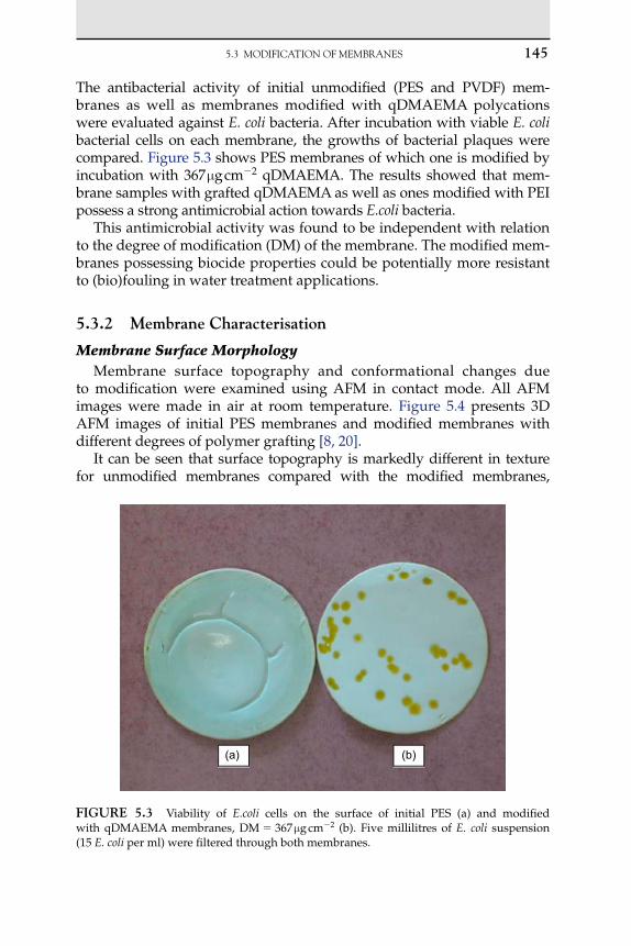
5.3 MODIFICATIONOFMEMBRANEs 145
The antibacterial activity of initial unmodified (PES and PVDF) mem-branes as well as membranes modified with qDMAEMA polycations were evaluated against E. coli bacteria. After incubation with viable E. coli bacterial cells on each membrane, the growths of bacterial plaques were compared. Figure 5.3 shows PES membranes of which one is modified by incubation with 367 g cm2 qDMAEMA. The results showed that mem-brane samples with grafted qDMAEMA as well as ones modified with PEI possess a strong antimicrobial action towards E.coli bacteria.
This antimicrobial activity was found to be independent with relation to the degree of modification (DM) of the membrane. The modified mem-branes possessing biocide properties could be potentially more resistant to (bio)fouling in water treatment applications.
5.3.2 Membrane Characterisation
Membrane Surface MorphologyMembrane surface topography and conformational changes due
to modification were examined using AFM in contact mode. All AFM images were made in air at room temperature. Figure 5.4 presents 3D AFM images of initial PES membranes and modified membranes with different degrees of polymer grafting [8, 20].
It can be seen that surface topography is markedly different in texture for unmodified membranes compared with the modified membranes,
(a) (b)
fIgurE 5.3 Viability of E.coli cells on the surface of initial PES (a) and modified with qDMAEMA membranes, DM 367 g cm2 (b). Five millilitres of E. coli suspension (15 E. coli per ml) were filtered through both membranes.

146 5. AFMANDDEvELOPMENTOF(BIO)FOULINg-REsIsTANTMEMBRANEs
although both are characterised by the same nominal pore size. The surface of grafted membrane having the lowest DM (shortest polymer chain length) appeared to have a laterally inhomogeneous structure consisting of clusters. As the DM increased (leading to an increased graft chain length), the clus-ters became higher and the grafted chain gathered into larger clusters.
Membrane Surface AnalysisFrom AFM images, surface analysis was carried out using instru-
ment software to obtain surface roughness parameters. The formation of the graft polymer layer on the membrane surface resulted in significant changes in surface morphology. Structural modifications become more pronounced with increasing DM. Figure 5.4 and Tables 5.1 and 5.2 pres-ent quantitative characteristics of the surface morphology of the initial and modified membranes derived from the AFM images [20].
The same trend can be observed in the roughness values for both PES and PVDF membranes. A slight increase in the membrane rough-ness compared with the unmodified membrane was observed for mem-branes modified with the lowest degree of grafted polymer (202 g cm2). At such a DM, grafted chains could be accommodated within the pores. Further increases in DM led to a significant increase in surface roughness with a layer of grafted polymer forming its own porous structure.
25 µm25 µm
25 µm25 µm
12.5 µm 12.5 µm
12.5 µm12.5 µm
0 µm 0 µm
0 µm0 µm Z scale = 720 nm Z scale = 720 nm
Z scale = 720 nmZ scale = 720 nm(a) (c)
(b) (d)
fIgurE 5.4 High-resolution 3D AFM images of initial (a) and modified with qDMAEMA (b)–(d) PES membranes; (b) DM 202 g cm2, (c) DM 367 g cm2 and (d) DM 510 g cm2.
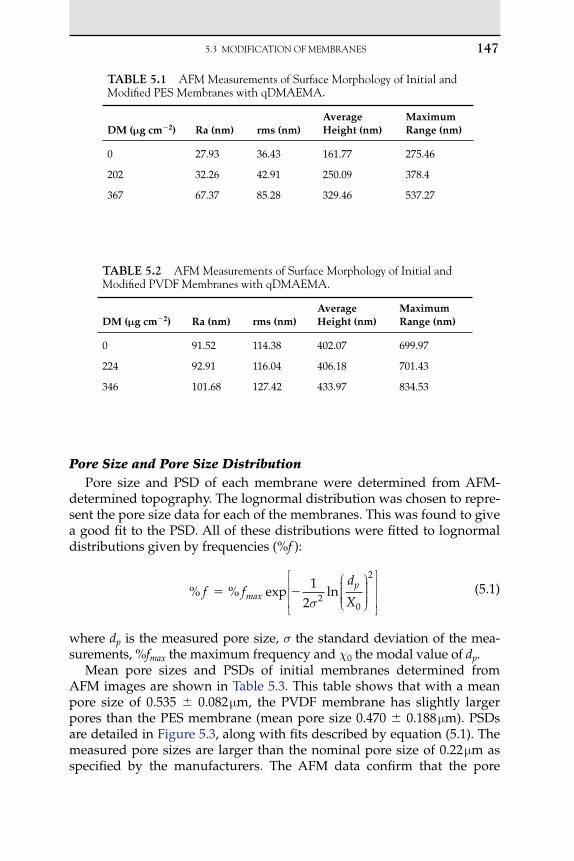
5.3 MODIFICATIONOFMEMBRANEs 147
Pore Size and Pore Size DistributionPore size and PSD of each membrane were determined from AFM-
determined topography. The lognormal distribution was chosen to repre-sent the pore size data for each of the membranes. This was found to give a good fit to the PSD. All of these distributions were fitted to lognormal distributions given by frequencies (%f ):
% exp lnfd
Xp
% fmax1
2 20
2
(5.1)
where dp is the measured pore size, the standard deviation of the mea-surements, %fmax the maximum frequency and 0 the modal value of dp.
Mean pore sizes and PSDs of initial membranes determined from AFM images are shown in Table 5.3. This table shows that with a mean pore size of 0.535 0.082 m, the PVDF membrane has slightly larger pores than the PES membrane (mean pore size 0.470 0.188 m). PSDs are detailed in Figure 5.3, along with fits described by equation (5.1). The measured pore sizes are larger than the nominal pore size of 0.22 m as specified by the manufacturers. The AFM data confirm that the pore
tAblE 5.1 AFMMeasurementsofsurfaceMorphologyofInitialandModifiedPEsMembraneswithqDMAEMA.
DM (g cm2) Ra (nm) rms (nm)Average Height (nm)
Maximum Range (nm)
0 27.93 36.43 161.77 275.46
202 32.26 42.91 250.09 378.4
367 67.37 85.28 329.46 537.27
tAblE 5.2 AFMMeasurementsofsurfaceMorphologyofInitialandModifiedPvDFMembraneswithqDMAEMA.
DM (g cm2) Ra (nm) rms (nm)Average Height (nm)
Maximum Range (nm)
0 91.52 114.38 402.07 699.97
224 92.91 116.04 406.18 701.43
346 101.68 127.42 433.97 834.53

148 5. AFMANDDEvELOPMENTOF(BIO)FOULINg-REsIsTANTMEMBRANEs
sizes of studied membranes are of approximately the same size. The topographical images give a clear perception of a notable difference in the surface morphology of the membranes used for the modification. A quantification of the surface parameters (Table 5.3) provides an insight into morphological particularities of these membranes which influence both the membrane separating properties and the process of modification by graft copolymerisation.
The two membranes under study have notably different PSDs. It can be noted here that PVDF has a narrower PSD with pore sizes from 0.336 to 0.68 m compared with a PSD ranging from 0.219 to 0.948 m in PES membranes. Moreover, these membranes significantly differ in sur-face roughness, with the PES membrane being smoother than the PVDF membrane. Regarding the AFM images, one might notice that the smoother surface allows for better contrast in pore observation, but more importantly the surface roughness is expected to have an influence on the graft copolymerisation.
The rate of membrane modification was higher in the case of PES membrane than PVDF membrane [19]. It is impossible to associate the difference only with the contribution of surface morphology. It is well known that polysulphone and PES are intrinsically photo-active, under-going bond cleavage with UV irradiation to produce free radicals even without the use of photo-initiators. PVDF is less photo-reactive than PES and produces less surface free radicals than PES. However, higher density of free radicals at the surface of more photo-reactive PES mem-branes also results in a higher probability of termination of chain growth and formation of cross-linked structures. These processes restricting an increase in the DM are competitive with respect to the chain growth. Since competitive processes, which enhance and decrease the amount of grafted polymer, occur simultaneously in the case of the photo-reactive polymer, the influence of surface morphology on graft copolymerisa-tion should not be discarded. For the relatively rough surfaces, such as PVDF membrane, the decrease in UV-irradiation effectiveness and steric hindrance for polymer growth in narrow valleys are possible effects that may decrease the modification to some degree.
tAblE 5.3 ParametersofPoresizeandPsDObtainedfromAFMImagesforInitialPEsandPvDFMembranes.
Pore size (m) PSD parametersMembrane Mean Minimum Maximum X0 (m) %fmax
PES 0.470 0.188 0.219 0.948 0.353 0.028 19.8 2.2 0.56 0.08

5.3 MODIFICATIONOFMEMBRANEs 149
Before detailed discussion of the quantitative characteristics of sur-face morphology, it is worth noting that the chosen lognormal pattern for PDS described by equation (5.1) gave a correlation coefficient of at least 0.95 for all fitted curves. The most probable pore sizes estimated from fitted curves were very close to the mean pore diameter calculated from corresponding sets of pore sizes for the initial and modified membranes (Tables 5.4 and 5.5).
According to Figure 5.5(a), the initial PES membrane has a very wide PSD with a value of 0.56 m. However, grafting of poly-qDMAEMA resulted in narrowing of the PSD and shifting the whole curve towards smaller pore sizes. As a result, mean pore size is gradually decreasing with the increase in the amount of poly-qDMAEMA grafted to the mem-brane surface. Significant improvement of the PSD was observed even for the modified PES membranes with the smallest DM (Table 5.4).
Narrowing of the PSD occurred mostly due to the disappearance of large pores (larger than 0.6 m). Taking into consideration that substantial narrowing of large pores demands higher quantities of grafted polymer
tAblE 5.4 AFMMeasurementsofPoresizeandPsDofInitialandModifiedPEsMembraneswithqDMAEMA.
Mean pore PSD parameters
DM (g/cm2) size (m) X0 (m) %fmax
0 0.470 0.188 0.353 0.028 19.8 2.2 0.56 0.08
202 0.337 0.098 0.278 0.010 41.4 4.4 0.32 0.04
367 0.293 0.072 0.281 0.003 51.3 2.0 0.26 0.01
510 0.100 0.083 0.075 0.004 26.9 2.9 0.40 0.05
tAblE 5.5 AFMMeasurementsofPoresizeandPsDofInitialandModifiedPvDFMembraneswithqDMAEMA.
Mean pore PSD parameters
DM (g/cm2) size (m) X0 (m) %fmax
0 0.535 0.082 0.555 0.003 51.2 1.7 0.14 0.01
224 0.445 0.083 0.439 0.018 35.1 4.1 0.28 0.02
346 0.334 0.079 0.297 0.013 44.3 5.7 0.30 0.01

150 5. AFMANDDEvELOPMENTOF(BIO)FOULINg-REsIsTANTMEMBRANEs
compared to smaller pores, it can be assumed that higher rates of poly-mer growth initiated at the walls of larger pores. As mentioned earlier, at the entrance of narrower pores, higher density of free radicals results in chain termination and consequently lower rate of polymer grafting. With time, when the PSD becomes more uniform, free radicals are even-tually distributed across the membrane surface. This leads to a gradual decrease of all surface pores with PSD shifting to smaller sizes. With DM higher than 202 m cm2, slight fluctuation in the width of PSD () was observed.
It can be seen from Table 5.5 that similar behaviour is observed regard-ing changes in the surface morphology of the PVDF membrane as for the PES membrane. However, the unmodified PVDF membrane has a more uniform PSD than the PES membrane. With a mean pore size approxi-mately 0.54 m, PSD of this membrane is characterised by a low value of , 0.14 m, compared with 0.56 m for PES membranes. Although modification of PVDF membrane with grafted qDMAEMA also led to PSD shifting towards lower pore sizes, PSD was wider for the modified membranes compared with initial membrane.
Pore size (µm)
Por
e de
nsity
%
00.0 0.00.1 0.10.2 0.20.3 0.30.4 0.40.5 0.50.6 0.60.7
0.0 0.1 0.2 0.3 0.4 0.5 0.6 0.7
0.8 0.9
0.02 0.04 0.06 0.08 0.10 0.12 0.14 0.16
1.0
5
10
40
15
20
2550
40
30
20
10
0
AFM dataFitted data
AFM dataFitted data
AFM dataFitted data
Pore size (µm)
Por
e de
nsity
%
10
0
20
30
30
15
10
5
0
20
25
Pore size (µm)
Por
e de
nsity
%
AFM dataFitted data
Pore size (µm)
Por
e de
nsity
%
(a) (c)
(d)(b)
fIgurE 5.5 PSDs of initial (a) and modified with qDMAEMA (b)–(d) PES membranes; (b) DM 202 g cm2, (c) DM 367 g cm2 and (d) DM 510 g cm2.

5.3 MODIFICATIONOFMEMBRANEs 151
5.3.3 (bio)Adhesion forces between a bSA-functionalised Colloid Probe and Membrane Surface
Adhesion force measurements were performed using the colloid probe technique. Colloid probes were prepared by immobilising modified microsphere with BSA to a tipless ultralever silicon cantilever.
Examples of retraction curves measured at three different loading forces for a BSA-modified microsphere interacting with a PES membrane grafted with qDMAEMA, shown in Figure 5.6, demonstrate that the adhe-sion force (pull-off force) increases with the force applied via the colloid [20]. Similar findings have been observed in previous studies [7, 14]. The increase in the adhesion force is most likely to result from an increase in the number of chemical bonds formed between the biopolymers when the
Loading force(mN m–1)
55
52
61
For
ce (
nNm
–1)
Separation (nm)
fIgurE 5.6 Representative approach (grey) and retraction (black) force curves of BSA-modified colloid probe to grafted membrane with qDMAEMA at different loading forces (pH 7).

152 5. AFMANDDEvELOPMENTOF(BIO)FOULINg-REsIsTANTMEMBRANEs
surfaces are forced into closer contact using higher loading forces [7]. In addition the deformation of the membrane surface at high loading forces may increase the area of contact between the probe and the membrane surfaces. In order to exclude the influence of loading force in comparison of interactions force, the experimental results are presented by plotting the adhesion force versus the loading force. For the purpose of comparison, the adhesion force at loading force equal to 80 mN m1 was measured, interpolated or extrapolated from the obtained experimental data.
Interactions Forces between Initial Membranes and Functionalised Colloid ProbesEffect of pH on Measured Adhesion Figure 5.7 shows the normalised adhesion force measurements versus the normalised loading force applied to the cantilever between a BSA-modified probe and initial PES membrane at different pH values. It can be seen that the adhesive force is highest at pH 5, followed by moderate values at pH 3 and the lowest at pH 7.
First, at pH 7 both the BSA and the membrane surface are negatively charged [21], which provoke increases in the repulsive electrostatic inter-action, leading to a reduction in adhesion. BSA is more hydrophobic at pH 5 than 7, which would be expected to increase adhesion. Secondly, the
Loading force (mN m–1)
Adh
esio
n fo
rce
(mN
m–1
)
040 60 80 100 120 140
2
4
6
8
10
12
pH=3 pH=5 pH=7
fIgurE 5.7 Relationship of adhesion and loading forces between initial PES and BSA probe in different pH solution. The dotted line is an extrapolated line.
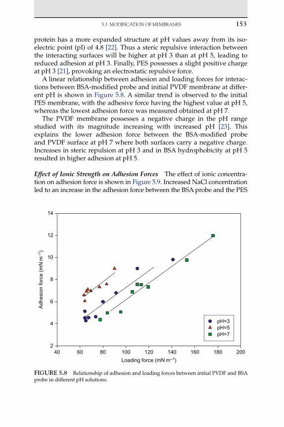
5.3 MODIFICATIONOFMEMBRANEs 153
protein has a more expanded structure at pH values away from its iso-electric point (pI) of 4.8 [22]. Thus a steric repulsive interaction between the interacting surfaces will be higher at pH 3 than at pH 5, leading to reduced adhesion at pH 3. Finally, PES possesses a slight positive charge at pH 3 [21], provoking an electrostatic repulsive force.
A linear relationship between adhesion and loading forces for interac-tions between BSA-modified probe and initial PVDF membrane at differ-ent pH is shown in Figure 5.8. A similar trend is observed to the initial PES membrane, with the adhesive force having the highest value at pH 5, whereas the lowest adhesion force was measured obtained at pH 7.
The PVDF membrane possesses a negative charge in the pH range studied with its magnitude increasing with increased pH [23]. This explains the lower adhesion force between the BSA-modified probe and PVDF surface at pH 7 where both surfaces carry a negative charge. Increases in steric repulsion at pH 3 and in BSA hydrophobicity at pH 5 resulted in higher adhesion at pH 5.
Effect of Ionic Strength on Adhesion Forces The effect of ionic concentra-tion on adhesion force is shown in Figure 5.9. Increased NaCl concentration led to an increase in the adhesion force between the BSA probe and the PES
Loading force (mN m–1)
Adh
esio
n fo
rce
(mN
m–1
)
240 60 80 100 120 140 160 180 200
4
6
8
10
12
14
pH=3pH=5pH=7
fIgurE 5.8 Relationship of adhesion and loading forces between initial PVDF and BSA probe in different pH solutions.

154 5. AFMANDDEvELOPMENTOF(BIO)FOULINg-REsIsTANTMEMBRANEs
membrane surface. The adhesion of the BSA probe to the initial unmodified PES increased by a factor of 2.4 across the concentration range 1–100 mM NaCl. This behaviour is qualitatively consistent with DLVO theory [24], as increasing the ionic strength compresses the thickness of the electrostatic double layer and should therefore reduce the repulsion force between the two surfaces, resulting in an increase in measured adhesion force.
The adhesion force measured between a BSA-coated probe and PVDF membrane surface at different ionic strength values is shown in Figure 5.10. As with the PES membrane, an increase in ionic strength led to an increase in the observed adhesion force. The adhesion force increased by a factor of 1.7 across the dissolved NaCl range of 1–100 mM. This is due to charge screening effects at higher ionic concentrations reducing the electrostatic repulsion, hence increasing the adhesion force between the interacting surfaces.
Comparison of (Bio)Adhesion Force Measurements between PES and PVDF Initial Membranes
Figure 5.11 shows the adhesion force for unmodified PES and PVDF membranes measured using BSA-coated colloid probes in solution at dif-ferent pH values. A similar trend was observed for the adhesion force as a function of pH for both membranes. However, the PVDF membrane
Loading force (mN m–1)
60 80 100 120
Adh
esio
n fo
rce
(mN
m–1
)
0
5
10
15
20
25
1 mM NaCl 10 mM NaCl 100 mM NaCl
fIgurE 5.9 Relationship of adhesion and loading forces between initial PES and BSA probe in different ionic strength solution at pH 5.8. The dotted line is an extrapolated line.
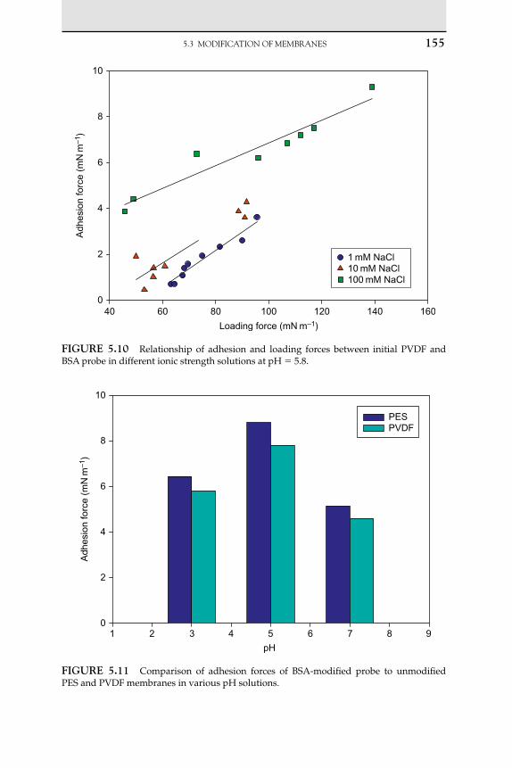
5.3 MODIFICATIONOFMEMBRANEs 155
Loading force (mN m–1)
Adh
esio
n fo
rce
(mN
m–1
)
040 60 80 100 120 140 160
2
4
6
8
10
1 mM NaCl 10 mM NaCl 100 mM NaCl
fIgurE 5.10 Relationship of adhesion and loading forces between initial PVDF and BSA probe in different ionic strength solutions at pH 5.8.
pH
Adh
esio
n fo
rce
(mN
m–1
)
01 2 3 4 5 6 7 8 9
2
4
6
8
10
PESPVDF
fIgurE 5.11 Comparison of adhesion forces of BSA-modified probe to unmodified PES and PVDF membranes in various pH solutions.

156 5. AFMANDDEvELOPMENTOF(BIO)FOULINg-REsIsTANTMEMBRANEs
showed a lower adhesion force than PES. This is most likely due to the PES membranes having a higher degree of hydrophobicity compared with PVDF. In addition, the PVDF membrane has a higher -potential than the PES membrane [21, 23]. Thus a higher repulsive electrostatic force would be expected between the probe and the unmodified PVDF membrane than unmodified PES membrane.
Effect of Ionic Strength A comparison of the adhesion force for both membranes as a function of ionic concentration is shown in Figure 5.12. In general a higher adhesion force is observed for PES membrane than PVDF membrane over the studied ionic strength range, except at ionic strength of 1 mM NaCl where adhesion force was small and no signifi-cant difference in adhesion of both membrane types is observed. At the highest ionic strength, the difference is the most dramatic. PES mem-brane is more hydrophobic than PVDF membrane. As a result a hydro-phobic attractive force leads to higher adhesion force for PES membrane than PVDF membrane.
Interactions Forces between Membranes Modified with qDMAEMA and BSA-Functionalised Colloid ProbeEffect of pH The effect of solution pH on adhesion force for PES mem-branes modified with qDMAEMA is shown in Figure 5.13. An increase in adhesion force with increasing pH was observed for modified membranes with three different DMs and is approximately threefold at a loading force of 80 mN m1.
The dominant contribution in the increase in adhesion force with increas-ing pH can be attributed to the electrostatic force between the positively charged modified membranes and the BSA probe. At pH 3 both surfaces (membrane and BSA probe) possess a positive charge resulting in greater repulsion at this pH and hence a lower adhesion than seen for other pH values. At pH 7 the modified PES membranes remains positively charged, whereas BSA carries a negative charge. This change in the nature of the electrostatic interaction leads to a greater observed adhesive force at pH 7.
Figure 5.14 shows the results for the effect of pH on the measured adhe-sion force of BSA to PVDF membrane functionalised with qDMAEMA. An increase in adhesion force with increasing solution pH was again observed. The experimental results for PVDF grafted with different DMs reveal the same trend. Taking into consideration the amphoteric behav-iour of BSA, which leads to a change in protein charge with changing pH, the BSA possesses a positive charge at pH values below the pI and a negative charge at pH values above the isoelectric point. This explains the relatively high adhesion at pH 7 where both the BSA and the mem-brane surface are oppositely charged. Thus, an attractive electrostatic force between the interacting surfaces results in higher adhesion.

5.3 MODIFICATIONOFMEMBRANEs 157
Ionic strength (mM)
0.1 1 10 1000
5
10
15
20
PESPVDF
Adh
esio
n fo
rce
(mN
m–1
)
fIgurE 5.12 Comparison of adhesion forces of BSA-modified probe to initial PES and PVDF membranes in various ionic strength solutions.
Loading force (mN m–1)
Adh
esio
n fo
rce
(mN
m–1
)
1
2
20 40 60 80 100 120 140
3
4
5
6
7
8
pH=3 pH=5 pH=7
fIgurE 5.13 Relationship of adhesion and loading forces between BSA probe and PES membrane modified with qDMAEMA (DM 510 g cm2) at different pH solution. The dotted line is an extrapolated line.

158 5. AFMANDDEvELOPMENTOF(BIO)FOULINg-REsIsTANTMEMBRANEs
Steric interaction could be another factor which plays a role in reduc-ing the adhesion force observed with both membranes at pH 3. The over-lap of the expanded protein layer and the modification of polymer chain of qDMAEMA, which is fully dissociated at this pH, enhance the repulsive interactions between the colloid probe and the surface of the modified mem-brane. In addition, at pH 5 there is practically no electrostatic interaction because this pH is close to the isoelectric point of the protein (the net charge is around zero) and, therefore, the electrostatic repulsion is negligible. As at pH 5 the protein has no net charge and so the structure of the protein is more compact and it has hydrophobic properties, such interaction may lead to high adhesion at pH 5 than at pH 3.
Effect of Ionic Strength Normalised adhesion forces versus normalised loading forces for interactions involving the modified PES membrane are shown in Figure 5.15 at different solution ionic strengths. An increase in adhesion force with increased ionic strength is evident.
The normalised adhesion force measured between BSA versus PVDF-modified membrane with qDMAEMA was examined as a function of ionic strength by varying the NaCl concentration (Figure 5.16). The adhesion force was also found to increase with increasing solution ionic strength. This is due to the compression of the double layer, which leads to the increase in adhesion force with increasing ionic strength.
Loading force (mN m–1)
Adh
esio
n fo
rce
(mN
m–1
)
0.060 70 80 90
0.5
1.0
1.5
2.0
2.5
3.0
3.5
pH=3 pH=5 pH=7
fIgurE 5.14 Relationship of adhesion and loading forces between BSA probe and PVDF membrane modified with qDMAEMA (DM 530 g cm2) in different pH solution.

5.3 MODIFICATIONOFMEMBRANEs 159
Comparison of (Bio)Adhesion Force Measurements Between Unmodified Membranes and Membranes Modified with qDMAEMAEffect of pH The normalised adhesion forces at the same loading force (loading force 80 mN m1) for initial and modified PES membranes with qDMAEMA are shown in Figure 5.17. It is clear that the unmodified membrane has a higher adhesion force than the modified membranes at pH 3 and 5, whereas the lowest adhesion was observed at pH 7. In addi-tion, at pH 3 modified membrane with the lowest DM exhibits the lowest adhesion. At pH 5 modified membrane with DM of 510 g cm2 showed the lowest adhesion force whereas both membranes show almost the same adhesion at pH 7.
The BSA-functionalised probe and both modified and unmodified membranes all possess a positive surface charge at pH 3. However, the qDMAEMA-functionalised membrane possesses a markedly greater charge than the unmodified PES membrane. The resulting greater elec-trostatic repulsion accounts for the greater adhesive forces observed with the initial unmodified PES membrane than with the modified membrane. When the surrounding solution is at pH 7, both the initial PES membrane and the BSA possess negative surface charges, with the qDMAEMA membrane still carrying a positive charge. This accounts for the modified membrane having a greater adhesive force with the BSA-coated probe than the unmodified membrane.
Loading force (mN m–1)
Adh
esio
n fo
rce
(mN
m–1
)
00 20 40 60 80 100 120
2
4
6
8
10
1 mM NaCl 10 mM NaCl 100 mM NaCl
fIgurE 5.15 Relationship of adhesion and loading forces between BSA probe and modified membrane with qDMAEMA (DM 510 g cm2) in different ionic strength solu-tions at pH 5.8. The dashed line is an extrapolated line.
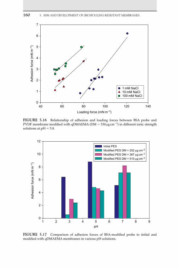
160 5. AFMANDDEvELOPMENTOF(BIO)FOULINg-REsIsTANTMEMBRANEs
Loading force (mN m–1)
Adh
esio
n fo
rce
(mN
m–1
)
040 60 80 100 120 140
1
2
3
4
5
6
7
1 mM NaCl 10 mM NaCl 100 mM NaCl
fIgurE 5.16 Relationship of adhesion and loading forces between BSA probe and PVDF membrane modified with qDMAEMA (DM 530 g cm2) in different ionic strength solutions at pH 5.8.
pH
Adh
esio
n fo
rce
(mN
m–1
)
01 2 3 4 5 6 7 8 9
2
4
6
8
10
12
Initial PES
Modified PES DM = 202 μg cm–2
Modified PES DM = 367 μg cm–2
Modified PES DM = 510 μg cm–2
fIgurE 5.17 Comparison of adhesion forces of BSA-modified probe to initial and modified with qDMAEMA membranes in various pH solutions.
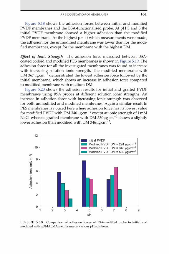
5.3 MODIFICATIONOFMEMBRANEs 161
Figure 5.18 shows the adhesion forces between initial and modified PVDF membranes and the BSA-functionalised probe. At pH 3 and 5 the initial PVDF membrane showed a higher adhesion than the modified PVDF membrane. At the highest pH at which measurements were made, the adhesion for the unmodified membrane was lower than for the modi-fied membranes, except for the membrane with the highest DM.
Effect of Ionic Strength The adhesion force measured between BSA-coated colloid and modified PES membranes is shown in Figure 5.19. The adhesion force for all the investigated membranes was found to increase with increasing solution ionic strength. The modified membrane with DM 367 g cm2 demonstrated the lowest adhesion force followed by the initial membrane, which shows an increase in adhesion force compared to modified membrane with medium DM.
Figure 5.20 shows the adhesion results for initial and grafted PVDF membranes using BSA probes at different solution ionic strengths. An increase in adhesion force with increasing ionic strength was observed for both unmodified and modified membranes. Again a similar result to PES membranes is noticed here where adhesion force has its lowest value for modified PVDF with DM 346 g cm2 except at ionic strength of 1 mM NaCl whereas grafted membrane with DM 530 g cm2 shows a slightly lower adhesion than modified with DM 346 g cm2.
pH
Adh
esio
n fo
rce
(mN
m–1
)
01 2 3 4 5 6 7 8 9
2
4
6
8
10
12
Initial PVDFModified PVDF DM = 224 μg cm–2
Modified PVDF DM = 348 μg cm–2
Modified PVDF DM = 530 μg cm–2
fIgurE 5.18 Comparison of adhesion forces of BSA-modified probe to initial and modified with qDMAEMA membranes in various pH solutions.

162 5. AFMANDDEvELOPMENTOF(BIO)FOULINg-REsIsTANTMEMBRANEs
Ionic strength (mM)
0.1 1 10 100
Adh
esio
n fo
rce
(mN
m–1
)
0
10
20
30
40
50
60Initial PESModified PES DM = 202 μg cm–2
Modified PES DM = 367 μg cm–2
Modified PES DM = 510 μg cm–2
fIgurE 5.19 Comparison of adhesion forces of BSA-modified probe to initial and modified with qDMAEMA membranes in solutions of increasing NaCl concentration.
Ionic strength (mM)
0.1 1 10 100
Adh
esio
n fo
rce
(mN
m–1
)
0
2
4
6
8
10
12 Initial PVDFModified PVDF DM = 224 μg cm–2
Modified PVDF DM = 348 μg cm–2
Modified PVDF DM = 530 μg cm–2
fIgurE 5.20 Comparison of adhesion forces of BSA-modified probe to initial and modified with qDMAEMA membranes in various ionic strength solutions.
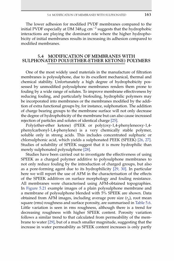
5.4 MODIFICATIONOFMEMBRANEswITHsULPHONATED 163
The lower adhesion for modified PVDF membranes compared to the initial PVDF especially at DM 348 g cm2 suggests that the hydrophobic interactions are playing the dominant role where the higher hydropho-bicity of initial membranes results in increasing its adhesion compared to modified membranes.
5.4 ModIfICAtIon of MEMbrAnES wIth SulPhonAtEd Poly(EthEr-EthEr KEtonE) PolyMErS
One of the most widely used materials in the manufacture of filtration membranes is polysulphone, due to its excellent mechanical, thermal and chemical stability. Unfortunately a high degree of hydrophobicity pos-sessed by unmodified polysulphone membranes renders them prone to fouling by a wide range of solutes. To improve membrane effectiveness by reducing fouling, and particularly biofouling, hydrophilic polymers may be incorporated into membranes or the membranes modified by the addi-tion of extra functional groups by, for instance, sulphonation. The addition of charge bearing groups to the membrane surface will not only decrease the degree of hydrophobicity of the membrane but can also cause increased rejection of particles and solutes of identical charge [25].
Poly(ether-ether ketone) (PEEK or poly(oxy-1,4-phenyleneoxy-1,4- phenylcarbonyl-1,4-phenylene) is a very chemically stable polymer, soluble only in strong acids. This includes concentrated sulphuric or chlorsulphonic acid, which yields a sulphonated PEEK (SPEEK) [26, 27]. Studies of solubility of SPEEK suggest that it is more hydrophilic than merely sulphonated polysulphone [28].
Studies have been carried out to investigate the effectiveness of using SPEEK as a charged polymer additive to polysulphone membranes to not only reduce fouling by the introduction of charged groups, but also as a pore-forming agent due to its hydrophilicity [29, 30]. In particular here we will report the use of AFM in the characterisation of the effects of the SPEEK additives on surface morphology and fouling resistance. All membranes were characterised using AFM-obtained topographies. In Figure 5.21 example images of a plain polysulphone membrane and a membrane of polysulphone blended with 5% SPEEK are shown. Data obtained from AFM images, including average pore size (rp), root mean square (rms) roughness and surface porosity, are summarised in Table 5.6. Little variation is seen in rms roughness, although there is a trend for decreasing roughness with higher SPEEK content. Porosity variation follows a similar trend to that calculated from permeability of the mem-brane to water [29], but of a much smaller magnitude, suggesting that the increase in water permeability as SPEEK content increases is only partly

164 5. AFMANDDEvELOPMENTOF(BIO)FOULINg-REsIsTANTMEMBRANEs
due to increase in the surface porosity. Changes in the thickness and/or the structure of the porous layer of the membrane may account for this.
Force measurements were also carried out between 4-m silica spheres and membranes. Figure 5.22 shows examples of typical data for force measurements taken from polysulphone membranes, with and with-out SPEEK present in 0.01 M NaCl. For the non-SPEEK membrane (P-P) the colloid probe snaps-in to the membrane surface, which indicates the pres-ence of long-range attractive forces, sufficient in magnitude to overcome the restoring force on the cantilever. This type of attraction leads to fouling
4.003.002.001.000.00
ÅÅ
300
200
100 100
200
300
0 0
Å
Å Å
2.00
1.00
0.00
300
200
300
200
100 100
0 0(b)
(a)
Å
fIgurE 5.21 AFM images of polysulphone membranes obtained with contact mode in air. (a) Polysulphone membrane and (b) polysulphone/SPEEK membrane (5% SPEEK pre-pared at 20°C). Roughness values were obtained from 2 2 m images.
tAblE 5.6 summaryofAFMCharacterisationDataforsPEEKModifiedPolysulfoneMembranes.
P-P S0.5-20 S2-20 S5-20 S2-10 S2-60
rp (nm) 0.93 0.15 0.89 0.22 0.93 0.15 0.73 0.18 1.05 0.22 0.86 0.26
rms roughness (nm)
3.2 4.2 3.5 2.5 3.1 2.1
Porosity, e (%) 6.0 9.0 14.1 16.9 15.1 12.8
Snap-in events (out of 9)
9 4 3 0 1 4
Foff, F/R (mN/m)
28.5 4.3 10.0 14.8 3.9 1.6 0.75 2.7 2.8 9.6 5.3

5.4 MODIFICATIONOFMEMBRANEswITHsULPHONATED 165
of the membrane. When the probe is retracted away from the membrane surface, a large attractive force is again measured. The difference between the attractive force at its greatest magnitude and the force measured when the probe has no net forces acting upon it (its free level) is the measured adhesion force, Foff. In contrast, for the S5-20 SPEEK membrane, no snap-in is observed. This is most likely due to the silica probe and membrane surface carrying charges which are identical in sign. When the particle is retracted, only a moderate adhesive force was measured. Data for the
2
1
0
0–2
20
FIR
/mN
m–1
40
ApproachRetraction
Distance/nm(b)
60
–1
5
–5
–10
–15
–20
0 20 40 60
–25
–30
FIR
/mN
m–1
ApproachRetraction
Distance/nm(a)
0
fIgurE 5.22 Example normalised force versus distance curves against (a) P-P type membrane and (b) S5-20 membrane.

166 5. AFMANDDEvELOPMENTOF(BIO)FOULINg-REsIsTANTMEMBRANEs
mean observed adhesion forces and the number of snap-in events mea-sured for each membrane are also tabulated in Table 5.6, based on the mea-surements taken from nine different points on each membrane surface. All measurements for P-P membrane contained snap-in events, but this decreased as the SPEEK content of the membrane increased. For the S5-20 membrane, containing 5% SPEEK, no snap-in event was measured at all. As the SPEEK content of the membranes is increased, a substantive and systematic decrease in mean observed adhesion forces is seen, being a fac-tor of almost 40 between P-P and S5-20 membranes. These trends together show the profound influence on the surface properties of the membranes of the incorporation of small amounts of SPEEK. It is also notable that the presence of snap-in events in some cases in the S-series membranes, except for S5-20, and the large standard deviation values show that some variabil-ity in the surface properties of the membranes exist.
AFM has also been used to help in the assessment of fouling by humic acid (HA) of SPEEK-modified polysulphone membranes [30]. HAs are heterogeneous materials, containing three main types of func-tional groups: carboxylic acids, phenolic acids and methoxycarbonyls. They are mostly negatively charged for pH values above pH 2.8 [31]. Measurements were carried out with the S5-20 SPEEK membrane, and an aromatic PES membrane (ES404), which were chosen as a comparable commercially available membrane [30].
The effects of a deposited HA layer on membrane filtration will depend to some extent on its physical state. Images of membranes ES404 and S5-20 prior to use in filtering HA from water are shown in Figure 5.23(a). Before use, the S5-20 membrane has a rougher surface, visible in the images, and also indicated by a greater rms roughness. Figure 5.23(b) shows images of the two same membranes after 2 h filtering HA from model water. For the ES404 membrane the deposit is compact with occasional larger spheroidal aggregates. The rms surface roughness was greater by a factor of approximately 1.9 compared to before filtra-tion. For the S5-20 SPEEK membrane, the deposit is much greater due to a higher flux [30]. The deposit is also less compact and more irregular than that seen for the ES404 membrane, and the rms surface roughness has increased by a factor of approximately 5.6 compared to before filtration. Both membranes were rinsed subsequent to filtration. Recovered mem-branes are shown in Figure 5.23(c). For the ES404 membrane, the surface roughness is similar to the fouled membrane, suggesting that rinsing has had little effect on removing the fouling aggregates. For the S5-20 mem-brane, however, the roughness value is greatly reduced from the fouled membrane, but has not quite returned to the value seen for the unused membrane. This suggests that most, but not all, of the fouling material has been removed by simple rinsing.

5.4 MODIFICATIONOFMEMBRANEswITHsULPHONATED 167
ES404: Rp-v 26.6 nm; Rrms 1.6 nm S5-20: Rp-v 33.7 nm; Rrms 2.5 nm
22
200 200
100 100
0 0
22
1 11 1
0(a) 00 0
1.5 1.51.51.5
0.5 0.50.5 0.5
Å Å
ES404: Rp-v 39.9 nm; Rrms 3.0 nm S5-20: Rp-v 124.0 nm; Rrms 14.1 nm
22
300200100
0
1000
800
400
0
1 1
(b) 0 0
1.51.5
0.5 0.5
22
1 1
0 0
1.51.5
0.5 0.5
Å
Å
(c)
S5-20: Rp-v 42.0 nm; Rrms 3.9 nm
Å400
300
200
100
0
µm
22
1.51.5
0.5 0.5
0 0
1 1
ES404: Rp-v 32.6 nm; Rrms 2.9 nm
300
200
0
100
2
1.5
Å
0.5 0.5
1
1.5
2
1µm µm µm
µmµm µm µm
µmµm µm µm
0 0
fIgurE 5.23 AFM images of ES404 and S5-20 membranes: (a) fresh membrane, (b) membrane after 2 h of filtering HA in water, and (c) recovered membrane after rinsing. Rp–v peak to valley roughness; Rrms rms roughness.

168 5. AFMANDDEvELOPMENTOF(BIO)FOULINg-REsIsTANTMEMBRANEs
The polymers from which the ES404 and S5-20 membranes are primar-ily constructed, PES and polysulphone, respectively, are similar in physical and chemical characteristics. However, the blending of SPEEK into the S5-20 has resulted in a greater surface charge, greater porosity and a greater roughness. These properties have also altered the way in which the HA deposits are structured. The much less compact nature of the HA layer on the S5-20 membrane has resulted in easier rinsing and cleaning, despite a higher deposition of material at the membrane surface.
Membranes containing blended SPEEK, such as the S5-20 membrane, show a combination of permeability, rejection properties and low adhe-sion characteristics. Attraction and adhesion to the membranes by silica colloids have been shown to be much reduced. In addition fouling by HA has been shown to be easily removed by simple rinsing of the membrane surface due to the open and un-compact structure of the deposited lay-ers. Further details of the development of PSU/SPEEK membranes are given in Chapter 4.
5.5 ConCluSIonS
In this chapter we have discussed the contribution that AFM may make in the development of biofouling-resistant filtration membranes. The ability to image the 3D topography of the membrane surface allows quantitative assessment of both roughness and PSD. Measurement of roughness before and after the use of a membrane gives a quantitative measure of the degree of fouling on the membrane and allows comparison between different membranes. The PSD gives an indication of porosity, which complements observations which may be made using other techniques. In addition the ability of the AFM to use the colloid probe technique to directly assess the interaction forces between colloids and membrane surfaces under differ-ent conditions is of great use when it comes to assessing the capability of newly developed membranes to reject fouling particulates.
In the future AFM has the capabilities to make a significant contribution in the development of new membrane surfaces and their properties, both by allowing characterisation of surface morphology and by measuring the physical interactions between membranes and potential fouling materials.
ACKnowlEdgEMEntS
We thank all who have contributed to this research, especially Laila Al-Khatib and Victor Kochkodan for their contribution to this research.

ABBREvIATIONsANDsyMBOLs 169
AbbrEvIAtIonS And SyMbolS
NOM Natural organic matterqDMAEMA Quaternary 2-dimethyl-aminoethylmethacrylatePES PolyethersulphonePVDF Polyvinylidene fluorideHEMA Hydroxyethyl methacrylateDM Degree of modificationdp Measured pore size (diameter) m Standard deviation of measurements0 Modal value of dp mPSD Pore size distributionBSA Bovine serum albuminSPEEK Sulphonated poly(ether-ether ketone)PEEK Poly(ether-ether ketone)HA Humic acid
references [1] N. Hilal, V. Kochkodan, L. Al-Khatib, G. Busca, Characterization of molecularly
composite membranes using an atomic force microscope, Surf. Interface Anal. 33 (2002) 672–675.
[2] M. Khayet, Membrane surface modification and characterization by X-ray photoelec-tron spectroscopy and contact angle measurements, Appl. Surf. Sci. 238 (1–4) (2004) 269–272.
[3] A.M. Mika, R.F. Childs, Acid/base properties of poly(4-vinylpyridine) anchored within microporous membranes, J. Memb. Sci. 152 (1) (1999) 129–140.
[4] M. Nystrom, S. Butylin, S. Platt, NF retention and critical flux of small hydrophilic/hydrophobic molecules, Memb. Technol. 10 (2000) 1–5.
[5] A.R. Costa, M.N. de Pinho, Effect of membrane pore size and solution chemistry on the ultrafiltration of humic substances solutions, J. Memb. Sci. 255 (1–2) (2005) 49–56.
[6] L.-C. Xu, B.E. Logan, Interaction forces between colloids and protein-coated surfaces measured using an atomic force microscope, Environ. Sci. Technol. 39 (10) (2005) 3592–3600.
[7] L.-C. Xu, V. Vadillo-Rodriguez, B.E. Logan, Residence time, loading force, pH, and ionic strength affect adhesion forces between colloids and biopolymer coated surfaces, Langmuir 21 (2005) 7491–7500.
[8] N. Hilal, W.R. Bowen, L. Al-Khatib, O.O. Ogunbiyi, A review of atomic force micro-scopy applied to cell interactions with membranes, Chem. Eng. Res. Design 84 (A4) (2006) 282–292.
[9] W.R. Bowen, N. Hilal, R.W. Lovitt, C.J. Wright, Direct measurement of the force of adhesion of a single biological cell using an atomic force microscope, Colloids Surf. A Physicochem. Eng. Asp. 136 (1998) 231–234.
170 5. AFMANDDEvELOPMENTOF(BIO)FOULINg-REsIsTANTMEMBRANEs
[10] W.R. Bowen, N. Hilal, R.W. Lovitt, C.J. Wright, Direct measurement of interactions between adsorbed protein layers using an atomic force microscope, J. Colloid Interface Sci. 197 (1998) 348.
[11] W.R. Bowen, N. Hilal, R.W. Lovitt, C.J. Wright, A new technique for membrane charac-terisation: direct measurement of the force of adhesion using an atomic force microscope, J. Memb. Sci. 139 (1998) 269–274.
[12] W.R. Bowen, N. Hilal, R.W. Lovitt, C.J. Wright, Characterisation of membrane surfaces: direct measurement of biological adhesion using an atomic force microscope, J. Memb. Sci. 154 (2) (1999) 205–212.
[13] W.R. Bowen, N. Hilal, R.W. Lovitt, C.J. Wright, An atomic force microscopy study of the adhesion of a silica sphere to a silica surface – effects of surface cleaning, Colloids Surf. A Physicochem. Eng. Asp. 157 (1999) 117–125.
[14] G. Toikka, R.A. Hayes, J. Ralston, Adhesion of iron oxide to silica studied by atomic force microscopy, J. Colloid Interface Sci. 180 (1996) 239–248.
[15] S. Veeramansunei, M.R. Yalamanchili, J.D. Miller, Measurement of interaction forces between silica and alpha-alumina by atomic force microscopy, J. Colloid Interface Sci. 184 (1996) 594–600.
[16] J.E. Kilduff, S. Mattaraj, J.P. Pieracci, G. Belfort, Photochemical modification of poly(ether sulfone) and sulfonated poly(sulfone) nanofiltration membranes for control of fouling by natural organic matter, Desalination 132 (1–3) (2000) 133–142.
[17] M. Taniguchi, G. Belfort, Low protein fouling synthetic membranes by UV assisted surface grafting modification: varying monomer type, J. Memb. Sci. 231 (1–2) (2004) 147–157.
[18] M. Ulbricht, H. Matuschewski, A. Oechel, H.G. Hicke, Photo-induced graft polymeriza-tion surface modifications for the preparation of hydrophilic and low protein-adsorbing ultrafiltration membranes, J. Memb. Sci. 115 (1) (1996) 31–47.
[19] L. Al-Khatib, Development of (bio)fouling resistant membranes for water treat-ment applications, in: School of Chemical, Environmental and Mining Engineering, University of Nottingham, 2006.
[20] N. Hilal, L. Al-Khatib, H. Al-Zoubi, R. Nigmatullin, Atomic force microscopy study of membranes modified by surface grafting of cationic polyelectrolyte, Desalination 185 (2005) 1025–1035.
[21] D. Kuzmenko, E. Arkhangelsky, S. Belfer, V. Freger, V. Gitis, Chemical cleaning of UF membranes fouled by BSA, Desalination 179 (1–3) (2005) 323–333.
[22] W.G. Liu, F. Li, X.D. Zhao, K.D. Yao, Q.G. Liu, Atomic force microscope characterisation forces between bovine serum albumin and cross-linked alkylated chitosan membranes in media of different pH, Polym. Int. 51 (12) (2002) 1459–1463.
[23] A.I. Schafer, U. Schwicker, M.M. Fischer, A.G. Fane, T.D. Waite, Microfiltration of colloids and natural organic matter, J. Memb. Sci. 171 (2) (2000) 151–172.
[24] J.A. Brant, Membrane colloid interactions: comparison of extended DLVO predictions with AFM force measurements, Environ. Eng. Sci. 19 (6) (2002) 413–427.
[25] W.R. Bowen, T.A. Doneva, Atomic force microscopy of membranes, in: A. Hubbard (Ed.), Encyclopedia of Surface and Colloid Science, Marcel Dekker, New York, 2002.
[26] A. Noshay, L.M. Robeson, Sulfonated polysulfone, J. Appl. Polym. Sci. 20 (1976) 1885–1903.
[27] M. Nystrom, P. Jarvinen, Modification of polysulfone ultrafiltration membranes with UV irradiation and hydrophilicity screening agents, J. Memb. Sci. 60 (1991) 275–296.
[28] T. Kobayashi, M. Rikukawa, K. Sanui, N. Ogata, Proton-conducting polymers derived from poly(ether-ether ketone) and poly(4-phenoxybenzoyl-1,4-phenylene), Solid State Ionics 106 (1998) 219–225.

REFERENCEs 171
[29] W.R. Bowen, T.A. Doneva, H.-B. Yin, Polysulfone – sulfonated poly(ethyl ether) ketone blend membranes: systematic synthesis and characterisation, J. Memb. Sci. 181 (2001) 253–263.
[30] W.R. Bowen, T.A. Doneva, H.-B. Yin, Separation of humic acid from a model surface water with PSU/SPEEK blend UF/NF membranes, J. Memb. Sci. 206 (2002) 417–429.
[31] S.-H. Yoon, J.-S. Kim, Effect of the origin of humic acids on nanofilter fouling in drink-ing water production, Chem. Eng. Sci. 55 (2000) 5171–5175.

6C H A P T E R
O U T L I N E
6.1 Introduction 173
6.2 The AFM as a Force Measurement Tool in Pharmaceuticals 1746.2.1 Particle Interaction Measurements 1756.2.2 Mechanical Properties from Single-particle Measurements 179
6.3 AFM Imaging-Based Studies 183
6.4 Micro- and Nanothermal Characterisation with SPM 185
6.5 Conclusions 190
Acknowledgements 190
Abbreviations and Symbols 190References 191
NanoscaleAnalysisofPharmaceuticalsby
ScanningProbeMicroscopyClive J. Roberts
6.1 INTroduCTIoN
There is an increasing demand to develop pharmaceuticals and bio-medical devices with architectures and complex chemistries controlled at the nanoscale. The need to develop delivery systems capable of target-ing specific sites in the body or to successfully formulate poorly soluble drugs frequently requires nanoscale solutions. For example, targeted sys-tems typically employ nanoparticles, incorporating a number of elements
Atomic Force Microscopy in Process Engineering ©2009,ElsevierLtd173

174 6. NANOSCALEANALySISOfPHARMACEUTICALSbySCANNINgPRObEMICROSCOPy
aimed at providing storage of the active therapeutic ‘stealth’ functional-ity to avoid the body defences as well as a targeting element. The addi-tional trend towards the delivery of protein- and DNA-based medicines through new alternative delivery routes such as inhalation has also increased this need for nanoscale analysis. Such complex systems require analysis capable of minimal disruption due to sample preparation and the ability to operate in a ‘physiological’ environment. This demand often exceeds the capacity of traditional analytical approaches to provide an effective understanding of this new generation of therapeutics.
This chapter will highlight the role of atomic force microscopy (AFM) and other scanning probe microscopies (SPM) in the qualitative and quantitative analysis of pharmaceuticals, highlighting both imaging and force data acquisition modes. These microscopes have enabled the study of pharmaceutical devices [1–3] and drug particles [4–6] with minimal pre-treatment in both air and liquid at the nanoscale level. The potential for SPMs, and AFM in particular, is now being exploited as an integral part of formulation, in both academic and industrial research. It is of course important to note that whilst SPM-based solutions do represent an increasingly important part of the analysis of pharmaceuticals, they are best applied with complementary approaches, such as Raman spectroscopy or diffraction-based techniques, which can provide chemically specific and 3D structural data.
6.2 The AFM AS A ForCe MeASureMeNT Tool IN PhArMACeuTICAlS
Most pharmaceuticals are produced as solid dosage forms (e.g. tablets, capsules, inhalable powders) and hence their manufacture inevitably involves the handling and manipulation of powdered materials. These powders can have particles ranging from submicron to many hundreds of microns in size. An understanding of how the mechanical properties of these particles and the forces between them influence factors such as processability and stability is an important feature of formulation devel-opment. Indeed, in some cases, the final form of the drug (and other materials in the medicine (the excipients)) is loose powder, as e.g. in a dry powder inhaler (DPI). Here then, the successful delivery of the drug itself relies on an intimate understanding of particle properties and their inter-actions. Until recently, the direct assessment of particle-particle and par-ticle-device interactions relied upon long-established bulk methods that deal with large numbers of particles, such as the centrifugal technique [7, 8]. Whilst effects such as cohesion and adhesion phenomena can be studied, these data reveal little concerning the nature and interplay of the

6.2 THEAfMASAfORCEMEASUREMENTTOOLINPHARMACEUTICALS 175
fundamental forces involved (e.g. van der Waals, electrostatic, capillary). Access to such information is beneficial not only to the assessment of a formulation, but also to establish the basis of any required particle modi-fication and optimisation.
Just as particle interactions can be probed using AFM, the nanoscale mechanical properties of powders can also be investigated. Previously, this could only be derived from bulk techniques, where powders are compressed into miniature beams and three-point bending tests are performed. The need for relatively large amounts of powder and to account for the porosity of the beams has limited the applicability of this approach. Even using miniaturised beams, milligram quantities of mate-rial are required, preventing screening of active pharmaceutical ingredi-ents at early stages of development [9, 10]. Here, we consider how AFM has been used to address both particle interactions and the measurement of the mechanical properties from single particles.
6.2.1 Particle Interaction Measurements
The ability to study single-particle interactions and the forces involved became possible with the advent of the AFM in 1986 [11–13]. In particu-lar, the use of AFM in the so-called ‘colloidal probe’ technique, whereby the force of interaction between a spherical bead attached to the AFM cantilever and a planar surface was studied, revealed the potential of this approach [14]. Importantly, a single particle (e.g. drug) attached to the AFM cantilever can be used for a series of comparative experiments chal-lenging different substrates. In addition, the ability of AFM to work in a variety of environments, such as controlled humidity and in liquids, is significant for pharmaceutical applications.
The first example of this approach being used for a pharmaceutical powder examined the differences in the adhesion of lactose particles to two gelatin DPI capsule surfaces [15]. It is important when attaching such individual drug particles to an AFM cantilever that their contact-ing region remains free from any adhesives employed or damage during attachment. An example scanning electron microscope (SEM) image is shown in Figure 6.1, where a drug particle is attached to an AFM cantile-ver. Typically, to prepare such a probe would involve the use of a minute amount of glue on the end of the cantilever to which a particle is attached using a micromanipulator or the AFM itself. This relatively labour-intensive sample preparation currently limits the number of different particles used within one study (usually to no more than five). The acces-sible particle size is typically in the range between 0.5 m and 50 m. For very small and/or cohesive particles (1 m or less), more than one may become attached to the lever; however, as long as only one comes into contact with the surface to be challenged, this is acceptable.

176 6. NANOSCALEANALySISOfPHARMACEUTICALSbySCANNINgPRObEMICROSCOPy
Having manufactured a particle probe, the forces of interaction of this probe with a surface are recorded. Figure 6.2 illustrates a schematic of a force curve and the main stages in acquiring such single-particle adhe-sion data. If such data is to be quantified in terms of force, then the spring constant of the AFM lever needs to be determined to enable cali-bration [16]. To ease comparisons between different-particle adhesion measurements, it is important to control key environmental factors such as humidity and to keep such instrument parameters as maximum press-on force, contact time, particle approach and retract speed constant.
Many researchers have now exploited this approach to explore particle interactions between drug and excipient particles and the components of delivery devices. Louey et al. used this approach to measure pull-off forces between a model colloidal silica probe and lactose particles suitable for use as carriers in a DPI [17]. AFM has also been used to rank the force of interaction of salbutamol with materials relevant to its inhaled delivery in the following manner, glass lactose salbutamol polytetrafluoroethylene (PTFE), showing that on PTFE tribocharging occurred following repeated contact [18]. Using AFM in this way has also revealed the effect of inducing amorphous content on the surface of particles of the drug zanamivir, where an increase in its affinity with a lac-tose carrier surface was observed [19]. Such surface amorphous material is important from a pharmaceutical perspective as this will be more soluble and probably less stable than a crystalline form of the drug, and hence can cause desirable (or undesirable) effects in terms of increased amounts of drug delivered on administration and stability problems in a medicine.
AFM cantilever
Drug particle
500 nm
FIgure 6.1 SEM image of the end of an AFM cantilever to which a single drug particle has been attached. The lower extremity of this particle forms the contact region with a sam-ple surface being studied within the AFM.

6.2 THEAfMASAfORCEMEASUREMENTTOOLINPHARMACEUTICALS 177
The influence of relative humidity on the forces between particles is an important consideration in pharmaceuticals as this can strongly influ-ence the stability of a medicine through the mediation of solution-based processes owing to surface adsorbed water. In addition, owing to the for-mation of capillary bridges between particles with increased humidity, this may cause aggregation. Hence, the effect of humidity has been the subject of a number of AFM studies. Young and co-workers have shown that drug cohesion increases at elevated humidity for some materials but decreased for others, potentially as a result of long-range attractive elec-trostatic interactions [20]. A variation in particle-contact morphology has also been shown to cause similar behaviour with increasing humidity [21]. The ability to record force data in controlled environments has been extended to work in liquids, e.g. to rank interactions in model propellants so as to simulate the environment within a pressurised metered dose inhaler [22–24].
AFM cantileverwith drug particle
Motion oflever
Sample
(a)
(b)
Particle approaching sample
Particle detachedto sample
Particle adheredto sample
0
0Relative veticle position of sample and particle (nm)
Can
tilev
er d
efle
ctio
n (n
m)
FIgure 6.2 (a) Schematic illustrating an AFM probe with attached drug particle com-ing to, contacting with and being removed from a sample surface. (b) With data recorded from such an event, the cantilever deflection can be converted to a force of the spring con-stant if the lever is known and the relative positions to a true sample-particle separation if the sensitivity of the microscope has been calibrated.
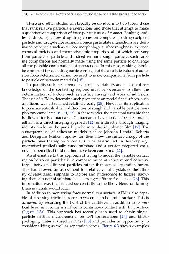
178 6. NANOSCALEANALySISOfPHARMACEUTICALSbySCANNINgPRObEMICROSCOPy
These and other studies can broadly be divided into two types: those that rank relative particulate interactions and those that attempt to make a quantitative comparison of force per unit area of contact. Ranking stud-ies address, e.g., how drug-drug cohesion compares to drug-excipient particle and drug-device adhesion. Since particulate interactions are dom-inated by aspects such as surface morphology, surface roughness, exposed chemical moieties and thermodynamic properties, all of which can vary from particle to particle and indeed within a single particle, such rank-ing comparisons are normally made using the same particle to challenge all the possible combinations of interactions. In this case, ranking should be consistent for each drug particle probe, but the absolute values of adhe-sion force determined cannot be used to make comparisons from particle to particle or between materials [18].
To quantify such measurements, particle variability and a lack of direct knowledge of the contacting regions must be overcome to allow the determination of factors such as surface energy and work of adhesion. The use of AFM to determine such properties on model flat surfaces, such as silicon, was established relatively early [25]. However, its application to pharmaceuticals due to difficulties of rough and variable particle mor-phology came later [19, 21, 22]. In these works, the principal variable that is allowed for is contact area. Contact areas have, to date, been estimated either via a direct imaging approach [22] or indirectly through imaging indents made by the particle probe in a plastic polymer film [19]. The subsequent use of adhesion models such as Johnson–Kendall–Roberts and Derjaguin–Muller–Toporov can then allow the surface energy of the particle (over the region of contact) to be determined. In this way, e.g., micronised (milled) salbutamol sulphate and a version prepared via a novel supercritical fluid method have been compared [22].
An alternative to this approach of trying to model the variable contact region between particles is to compare ratios of cohesive and adhesive forces between different particles rather than actual separation forces. This has allowed an assessment for relatively flat crystals of the affin-ity of salbutamol sulphate to lactose and budesonide to lactose, show-ing that salbutamol sulphate has a stronger affinity for lactose [26]. This information was then related successfully to the likely blend uniformity these materials would form.
In addition to monitoring force normal to a surface, AFM is also capa-ble of assessing frictional forces between a probe and a surface. This is achieved by recording the twist of the cantilever in addition to its ver-tical bend as it scans a surface in continuous contact with that surface (Figure 6.3a). This approach has recently been used to obtain single-particle friction measurements on DPI formulations [27] and blister packaging material (used in DPIs) [28] and provides an opportunity to consider sliding as well as separation forces. Figure 6.3 shows examples
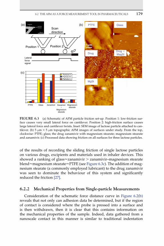
6.2 THEAfMASAfORCEMEASUREMENTTOOLINPHARMACEUTICALS 179
of the results of recording the sliding friction of single lactose particles on various drugs, excipients and materials used in inhaler devices. This showed a ranking of glasszanamivir zanamivir–magnesium stearate blendmagnesium stearatePTFE (see Figure 6.3c). The addition of mag-nesium stearate (a commonly employed lubricant) to the drug zanamivir was seen to dominate the behaviour of this system and significantly reduced the friction [27].
6.2.2 Mechanical Properties from Single-particle Measurements
Consideration of the schematic force distance curve in Figure 6.2(b) reveals that not only can adhesion data be determined, but if the region of contact is considered where the probe is pressed into a surface and is then withdrawn, then it is clear that this contains information on the mechanical properties of the sample. Indeed, data gathered from a nanoscale contact in this manner is similar to traditional indentation
PTFE Glass Zanamivir Zanamivir�
Magnesiumstearate
Magnesiumstearate
Particle AParticle BParticle C
Position 1 Position 2
Scandirection
Lateralforcesignal
(a) (b)
(c)
PTFE
DrugDrug �MagSt
MgSt
Glass
FIgure 6.3 (a) Schematic of AFM particle friction set-up. Position 1: low-friction sur-face causes very small lateral force on cantilever. Position 2: high-friction surface causes large lateral force and cantilever twists. Inset: SEM image of lactose particle attached to can-tilever. (b) 5 m 5 m topographic AFM images of surfaces under study. From the top, clockwise: PTFE; glass; the drug zanamivir with magnesium stearate; magnesium stearate and zanamivir. (c) Processed data showing friction on all surfaces for three lactose particles.

180 6. NANOSCALEANALySISOfPHARMACEUTICALSbySCANNINgPRObEMICROSCOPy
measurements more typically measured on a micron or greater scale to determine elastic modulus and hardness [29]. There are, however, a num-ber of limitations of the AFM data that must first be considered. First, as standard AFM cantilevers are typically very flexible (so that they are sensitive to nanoNewton forces), they are incapable of deforming sur-faces beyond approximately 10 GPa elastic modulus. Second, unlike a traditional indenter, an AFM probe does not approach or deform a sur-face completely normal to that surface, because of the need to have the lever at a slight angle to ensure that the probe apex contacts the sample first. This causes lateral deformation errors in the data, which are only negligible with relatively small indent depths.
Despite these issues, many groups have employed AFM to determine the elastic, inelastic and hardness properties of materials. Such deformation behaviour of pharmaceutical ingredients is known to affect pharmaceu-tical processes such as milling and compaction [30–33]. To date, most reported pharmaceutical examples of this approach have used a modi-fied AFM equipped with a relatively large probe with well-defined geometry and a much stiffened spring that supports this probe [30, 34, 35]. Typically, in these methods, material parameters are extracted from load-displacement unloading curves using approaches outlined by Oliver and Pharr [36]. Recently, Ward and co-workers [37] have utilised a sharp AFM probe and normal cantilevers to record nanomechanical measurements on sorbital samples to quantitatively distinguish between amorphous and crystalline domains through Young’s modulus mea-surements. Figure 6.4 shows images and typical force distance curves obtained from crystalline and amorphous sorbitol regions and a control of a hard, non-indenting silicon substrate. To determine the nanoin-dentation of the probe tip into the sorbitol sample as a function of load, the force distance curves from the sorbitol sample and the control hard substrate were compared. When comparing the amorphous and the crystalline regions, it is the amorphous region that provided the greater deflection of the tip (indicating the softer material and greater indenta-tion) at the given applied loads [37]. In this approach, a comparison of the gradients of the contact region of the force distance curves between a hard non-deformable reference surface and the sample can provide the relative stiffness of a surface [38]. By applying the Hertz model [39] to the nanoindentation data, a quantitative value of the Young’s modulus of the surfaces can be obtained. The Hertz model describes the elastic defor-mation of two homogenous surfaces under an applied load and is often used to model AFM data since it requires little knowledge of parameters such as surface energy. The first step in modelling the data is to compare force distance curves recorded on the sample and an ideally hard refer-ence (glass surface) to determine the indentation () of the probe into the sample as a function of load. The contact regions of the curves are over-laid such that zero force is equal to zero indentation.
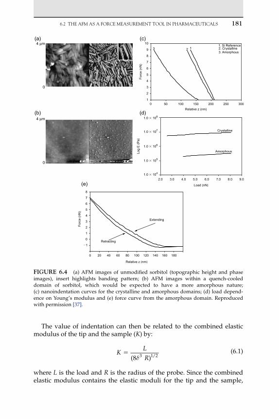
6.2 THEAfMASAfORCEMEASUREMENTTOOLINPHARMACEUTICALS 181
The value of indentation can then be related to the combined elastic modulus of the tip and the sample (K) by:
K
LR
( )8 3 1 2 /
(6.1)
where L is the load and R is the radius of the probe. Since the combined elastic modulus contains the elastic moduli for the tip and the sample,
10
9
8
7
6
5
4
3
0
0
0
50 100 150 200 250 300
2
1
Relative z (nm)
1.0 � 108
1.0 � 107
1.0 � 106
1.0 � 105
1.0 � 104
2.0 3.0 4.0 5.0 6.0 7.0 8.0 9.0
Load (nN)
Log
E (P
a)Fo
rce
(nN
)
Amorphous
Crystalline
8
7
6
5
Forc
e (n
N)
3
4
2
1
0
0 20 40 60
Relative z (nm)
80 100 120 140 160 180
�1Retracting
Extending
(a)
(b)
(e)
(d)
(c)4 µm
4 µm
3 2 11. Si Reference2. Crystalline3. Amorphous
FIgure 6.4 (a) AFM images of unmodified sorbitol (topographic height and phase images), insert highlights banding pattern; (b) AFM images within a quench-cooled domain of sorbitol, which would be expected to have a more amorphous nature; (c) nanoindentation curves for the crystalline and amorphous domains; (d) load depend-ence on Young’s modulus and (e) force curve from the amorphous domain. Reproduced with permission [37].

182 6. NANOSCALEANALySISOfPHARMACEUTICALSbySCANNINgPRObEMICROSCOPy
an expression containing the Es, the elastic moduli of the sample can be obtained:
K
E Et
t
s
s
43
1 12 2 1υ υ
(6.2)
where νt and νs are the Poisson’s ratio of the tip and the sample, respec-tively. Since Et is much greater than Es, the first term in the bracket of equation (6.2) may be ignored to produce equation (6.3):
E
Ks
s3 14
2( )υ
(6.3)
Combining equations (6.1) and (6.3) derives:
E
LRs
s3 1
4 8
2
3 1 2( )
( )υ
/
(6.4)
The value of νs is difficult to determine accurately for many samples such as sorbitol and other pharmaceutical materials. Therefore, it is appropriate to use a midrange value of νs (typical range is from 0.1–0.5) since varying this has little effect on the value obtained for Es.
The Hertz model is valid only for elastic deformation, so it is important to remove any contribution from inelastic deformation from the analysis. The model also assumes no significant adhesion between the probe and sample. To overcome this, only data from the loading curve is typically used. To assess the validity of the data for use with the Hertz model, a plot of load versus indentation is typically produced. In the ideal situation, a lin-ear relationship between load and indentation should be observed to allow Es to be calculated. The Young’s modulus values for the amorphous regions of the sorbitol using this type of analysis of Ward et al. were less than the crystalline regions [37]. Interestingly, the Young’s modulus values appeared to rise with increases in loading in both amorphous and crystalline regions of sorbital, suggesting possible viscoelastic/plastic deformation [37]. Hence, these surface mechanical measurements were able to distinguish between crystalline and amorphous material and exemplify the possible use of the AFM to screen batch-to-batch variations in drug formulations.
In general, it can be seen, therefore, that AFM provides a very flexible platform, adaptable to a range of experimental geometries for force mea-surements with real pharmaceutical materials. Examples of determining the interaction between an iron-coated AFM probe and a range of drugs to simulate tablet press–tablet interactions [40], and particle-bubble inter-action forces in the mineral processing industry [41] give an idea of other possibilities yet to be fully explored.

6.3 AfMIMAgINg-bASEdSTUdIES 183
6.3 AFM IMAgINg-BASed STudIeS
As a microscopy, AFM is perhaps better known for its ability to image surfaces at nanometre resolution in a variety of environments than as a force measurement tool. As a material under study can be exposed to environmental stresses (temperature, humidity, solvents etc.), it can often be in a dynamic state and hence, as long as the kinetics are not too rapid, AFM is able to provide a dynamic view of surface-mediated processes (unless employing advanced video rate imaging AFM [42], a typical 1 m 1 m image takes approximately 30 s to acquire). This approach has found effective applications in pharmaceuticals in the study of envi-ronmental stress on the surface properties of formulations, drug release from erodible materials and crystallisation phenomena.
Price and Young [43] have studied the real-time effects of changes in relative humidity (RH) on spray-dried lactose using environmentally controlled AFM. The lactose was imaged at 0%, 30% and 58% RH for 4, 2 and 22 h, respectively. Recrystallisation of amorphous lactose, promoted by the presence of water, was observed at 58% and 75% RH, although only some of the particles were shown to undergo nucleation and crys-tal growth. The AFM data was combined with traditional approaches such as X-ray powder diffraction, differential scanning calorimetry and dynamic vapour sorption and was shown to have significant potential for studies of the nucleation and crystallisation processes of amorphous material [43].
Li and co-workers have utilised contact mode AFM imaging in air to image a series of partial dissolutions on the (010) face of paracetamol [44]. From the AFM images of the (010) face of acetaminophen crystals treated with alternative dissolution solvents, different etching patterns were observed. These different etching patterns were speculated to be a result from the surface diffusion of the crystal molecules desorbed dur-ing the dissolution process and by the mutual interaction between the solvent and crystal molecules. AFM has similarly been employed to visualise the effect of dissolution media on various polymeric systems designed to achieve a specific drug-release profile [45].
It is widely known that pharmaceutical additives and impurities in drug formulations can affect drug crystal growth, morphology and poten-tial drug efficacy. This may be achieved deliberately to control crystal habit or an undesirable consequence of contamination. By understanding the degree to which impurities affect these critical formulation parame-ters, drug delivery systems can be developed more effectively. AFM has the capability to study drug crystal changes in real time, as demonstrated by Thompson et al. in the study of paracetamol in the presence of impu-rities, acetanilide and metacetamol using AFM in liquid [46]. A series of real-time AFM images of the (001) face of a native paracetamol crystal are

184 6. NANOSCALEANALySISOfPHARMACEUTICALSbySCANNINgPRObEMICROSCOPy
shown in Figure 6.5, and illustrates that the growth steps of crystallisa-tion over 4.8 h are curved in appearance, indicative of crystal growth via the screw dislocation mechanism. AFM images of the (001) face of another paracetamol crystal during incubation with 4 mol% acetanilide over time are shown in Figure 6.6. The defects in the crystal surface form weak points, leading to deepened holes (one hole is highlighted by a black arrow in Figure 6.6) over 12 h, indicating that the dissolution occurs both laterally and towards the crystal core [46]. Images during incubation with 4 mol% metacetamol showed that the steps formed were significantly smaller and pointed in appearance (image not shown here). These fea-tures were ascribed to ‘pinning’, an effect caused when additives adsorb onto the steps and force them to grow between the impurities [46].
From our consideration of AFM as a force measurement tool, it is clear that the probe is sensitive not only to topography but also to the magni-tude and nature of the forces experienced by the probe. Consequently, whilst imaging, if such sensitivity can be mapped also, it becomes possi-ble to produce alongside topography data sensitive to a particular surface property (e.g. adhesion, harness etc.). For example, during the commonly employed tapping mode imaging [47], where the AFM cantilever is oscil-lated at its resonant frequency and intermittently contacts a sample surface at the bottom of each oscillation cycle, the phase of the oscillation as well as
FIgure 6.5 A sequence of 10 m 10 m AFM images of the (001) face of a paraceta-mol crystal during incubation in paracetamol solution. In image (a) time t 0 s, (b) t 60 s, (c) t 118 s, (d) t 176 s, (e) t 234 s and (f) t 292 s. Figure reproduced with permission [46].

6.4 MICRO-ANdNANOTHERMALCHARACTERISATIONwITHSPM 185
the topography can be recorded. Phase images are obtained by measuring the phase lag between the signal that drives the cantilever-tip oscillation and the output signal of the cantilever oscillation (will differ more to the original cantilever-tip oscillation if the sample surface is soft and visco-elastic due to greater energy lost to the sample). The use of phase imaging alongside topographical imaging is particularly useful for studying drug polymorphs phase-separated systems and drug-excipients systems as it can be used to map out a profile of materials with different mechanical and physicochemical properties [48, 49].
6.4 MICro- ANd NANoTherMAl ChArACTerISATIoN wITh SPM
Knowledge of the distribution and physical form of a drug in its formulation is important in determining its overall performance and can further our understanding into bioavailability issues in medicines. Classically, one of the main tools used to identify the form a drug takes within a formulation and the interactions between its components is
FIgure 6.6 A sequence of 10 m 10 m AFM images of the (001) face of a para-cetamol crystal in paracetamol/4 mol% acetanilide solution. The dissolution of step one is followed by a black arrow on each image. Image (a) is taken 11.5 min after addition of paracetamol/4 mol% acetanilide solution. Images (b–f) are taken at the following times after image (a): (b) t 146 s, (c) t 290 s, (d) t 436 s, (e) t 582 s and (f) t 728 s. Figure reproduced with permission [46].

186 6. NANOSCALEANALySISOfPHARMACEUTICALSbySCANNINgPRObEMICROSCOPy
calorimetry. However, such approaches cannot reveal the spatial distribu-tion of these components. An adaptation of AFM that can achieve this is the Scanning Thermal Microscope (SThM) [50]. Here, the normal silicon cantilever is replaced with a Wollaston wire probe, brought to a sharp apex in the form of a cantilever. The spatial (and thermal mapping) reso-lution of such probes is on the order of a micron. Whilst this is useful, they also have the additional ability to apply heat locally to a surface and to record the power required to deliver a constant temperature increase to that point in the sample (in a manner analogous to Differential Scanning Calorimetry (DSC)), therefore providing detailed thermal characterisation at that point on a sample (the so-called Local Thermal Analysis (LTA)). To date, LTA has been the main area of application of this approach in pharmaceuticals.
Six et al. have demonstrated the ability of SThM analysis to distin-guish and identify phase-separated material in solid dispersions of itraconazole and Eudragit® E100 polymer [51]. Such dispersions of a poorly soluble drug in a soluble matrix represent a classic route to improving the bioavailability of such drugs. SThM images of disper-sions containing 10%, 40% and 60% itraconazole showed an increase in surface roughness with an increase in drug loading, possibly linking the rough surface areas to phase-separated drug. Phase-separated regions of the drug are not desired as they would be less liable to release the active ingredient than molecular dispersed drug. LTA has been used to charac-terise the different phases by a comparison of the glass transition (Tg) of different dispersions with that of the pure compounds of drug and poly-mer. LTA showed that the penetration of the probe tip into a sample of pure itraconazole occurred at around 333 K, which is in good agreement with the previously determined Tg for the drug by DSC of 332.4 K. In con-trast, the penetration of the probe tip into pure Eudragit® E100 occurred at a much higher temperature of 383 K compared to its Tg of 318 K deter-mined by DSC and was linked to the fragility of the sample [51]. It was also observed in dispersions with low drug loading (10%) that the probe-tip penetration was at a temperature in between the Tgs for itraconazole and Eudragit® E100, an indication of intimate mixing of the components. At high drug loading (60%) dispersions, the Tg was similar to that for the drug, indicating separation of the components.
In another study by Sanders et al. [52], SThM combined with LTA was used to distinguish between two polymorphs of cimetidine, types A and B. These two pharmaceutically useful anhydrous polymorphs of cimetidine had previously been tentatively distinguished by AFM phase imaging in a variable humidity environment [48]. An understanding and ability to detect and distinguish between different polymorphs in drug formulations is of particular significance, as different polymorphs can have different physicochemical properties and can convert from one

6.4 MICRO-ANdNANOTHERMALCHARACTERISATIONwITHSPM 187
form to another under storage conditions. While cimetidine is known to have seven polymorphs, only type A and type B are used in tablet and suspension formulations, respectively [53]. SThM images were obtained using a probe temperature of 50°C and a scan rate of 1 Hz. Figure 6.7 shows topographical (images a and c) and SThM images (images b and d) of a 50:50 mixture of polymorph type A and type B from two different areas. The contrast highlighted by arrows in images b and d is a result of the differences in surface thermal conductivity in the two different poly-morphs. LTA on discs of pure samples of polymorphs type A and type B were used to help elucidate that the lighter and darker regions observed in the topographical data (Figure 6.7a, c) were of polymorphs type A and
FIgure 6.7 50 m 50 m images of a pressed disc comprising a 50:50 mixture of the A and B polymorphs of cimetidine (scale bar: 10 mm): (a) and (c) show topographical images of two different areas of the disc and (b) and (d) show the corresponding thermal conductivity images. Features highlighted with arrows show contrast as a result of the differing thermal behaviour of the two polymorphic forms of cimetidine. Reproduced with permission [52].

188 6. NANOSCALEANALySISOfPHARMACEUTICALSbySCANNINgPRObEMICROSCOPy
type B, respectively. LTA was performed with a temperature ramp rate of 10°C s1. Figure 6.8 shows the local thermal analysis of polymorphs B and A with melting points observed between 140–146°C and 141–143°C, respectively. The close range of melting points for polymorphs A and B illustrates why bulk thermal analytical methods have difficulty distin-guishing between the two polymorphs. An interesting feature of the data for polymorph A is the endothermic peak seen just above 100°C (marked X in Figure 6.8b). This feature is seen in neither the bulk thermal analysis of form A nor LTA of form B. This would suggest that this feature is a result of the increased surface sensitivity of the localized measurements, and that this endothermic peak is likely to be a result of adsorbed surface water. This is consistent with form A being more hydrophillic than form
0
1.5
0
1
Sen
sor
mov
emen
t (μ
m)
Sen
sor
mov
emen
t (μ
m)
0
–1
–2
–2
–2
–4
–2
–1.5
–3
20
20 60 100 140
60
Temperature (°C)
Temperature (°C)
100 180
1
0
1
Der
iva
tive
pow
er (μ
Wde
g–1 )
Der
iva
tive
pow
er (μ
Wde
g–1 )
(IV)
(IV)
(II)
(III)
(I)
(III)
(I)
(II)
(a)
(b)
FIgure 6.8 Localised thermal analysis of pure cimetidine polymorphs (a) B and (b) A. Lines denoted (I) show the calorimetric data for a single point and dashed lines (II) show the movement of the sensor during the measurement, corresponding to thermomechanical analysis. Lines (III) and (IV) show similar data for other points on the samples. Reproduced with permission [52].

6.4 MICRO-ANdNANOTHERMALCHARACTERISATIONwITHSPM 189
B and with previous AFM data, which displayed a behaviour indicative of adsorbed water at the surface [48].
These and other results not only demonstrate the ability of LTA to ther-mally characterise individual components within formulation mixes, but also highlight the limitation of the system to detect structures of approx-imately 20 m 20 m or larger, such that if more than one structure is present in a region, the LTA measurement appears as an intermediate softening of values between individual components.
Clearly, replacement of the traditional AFM imaging probe with a heat-conductive Wollaston wire has enabled the local thermal properties of pharmaceuticals to be investigated but at the sacrifice of spatial reso-lution. However, the recent development of a commercially fabricated doped-silicon cantilever with a heated probe has enabled this problem to be overcome and for nanoscale thermal events with nanometre preci-sion to be probed [54]. This nanothermal cantilever has a conductive coat-ing through which an electrical current is passed to an integrated heater located directly above the probe. By varying the resistance of the circuit, the temperature of the heater can be controlled up to 500°C, depending on the choice of probe. When the probe is in contact with the surface, any deflections in the cantilever are recorded and this can reveal the nature of the material (e.g. amorphous versus crystalline) [55, 56] and the occur-rence of thermal phase transitions such as melting or glass transitions [54]. The development of the nanoprobe has also given the ability to maintain a constant probe temperature during scanning to allow for thermal imag-ing of the surface or for controlled thermal nanolithography [57, 58]. An example of such local thermal analysis is shown in Figure 6.9, where an
Dehydration
Melt
50 100 150 200Temperature (°C)
Def
lect
ion
(arb
. uni
ts)
FIgure 6.9 Nanoscale thermal analysis (NTA) of lactose monohydrate. (Left) Image recorded with an NTA probe after local thermal analysis has been performed at the area, high-lighted with an arrow. The nanoscale pit is the result of local melting. (Right) Corresponding cantilever deflection trace, revealing dehydration and melting of the lactose monohydrate.

190 6. NANOSCALEANALySISOfPHARMACEUTICALSbySCANNINgPRObEMICROSCOPy
individual lactose monohydrate crystal within a blend has been studied. The resultant indent due to local melting is apparent in the image (now with nanometre resolution due to the sharper probe). The corresponding cantilever deflection trace reveals the loss of water from the monohydrate and the melt of the anhydrous form at temperatures consistent with pre-vious SThM and bulk analysis [59].
6.5 CoNCluSIoNS
As the barriers to developing new medicines become ever greater owing to new challenges in delivery, greater regulation and the scarcity of ‘easy’ molecules to develop into medicines, the role of probe micro-scopes in pharmaceuticals development is set to increase. The advantages of nanoscale resolution, minimal sample preparation and the non-invasive imaging capabilities of AFM in particular make this an ideal tool to bring new approaches to the investigation of drug material properties.
This chapter has provided an insight into the improved understand-ing of pharmaceutical drug development available by AFM and thermal versions of AFM. These approaches have in a relatively short period of time provided a series of new insights into drug particle interactions and formulation structure. The capacity of AFM to not only image at the nanoscale but also to investigate interactions and to spatially map sur-face properties and to operate in a variety of environments consistent with pharmaceutical testing, manufacture and delivery provides great opportunity.
ACkNowledgeMeNTS
I would like to thank all who have contributed to this research, espe-cially Martyn Davies, Jennifer Hooton, Ardeshir Danesh, Jin Zheng, Jeff James, Matthew Bunker, Michael Davies and Anne Turner.
ABBrevIATIoNS ANd SyMBolS
DPI dry powder inhaler
Es elastic modulus of sample N m2
K combined elastic modulus of tip and sample N m2
L load force N
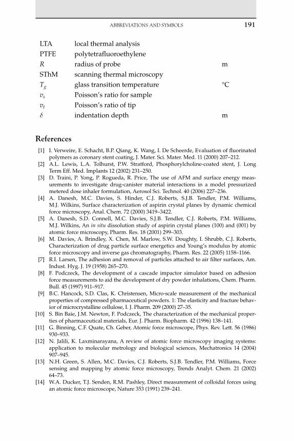
AbbREvIATIONSANdSyMbOLS 191
LTA local thermal analysisPTFE polytetrafluoroethyleneR radius of probe mSThM scanning thermal microscopyTg glass transition temperature °Cvs Poisson’s ratio for samplevt Poisson’s ratio of tip indentation depth m
references [1] I. Verweire, E. Schacht, B.P. Qiang, K. Wang, I. De Scheerde, Evaluation of fluorinated
polymers as coronary stent coating, J. Mater. Sci. Mater. Med. 11 (2000) 207–212. [2] A.L. Lewis, L.A. Tolhurst, P.W. Stratford, Phosphorylcholine-coated stent, J. Long
Term Eff. Med. Implants 12 (2002) 231–250. [3] D. Traini, P. Yong, P. Rogueda, R. Price, The use of AFM and surface energy meas-
urements to investigate drug-canister material interactions in a model pressurized metered dose inhaler formulation, Aerosol Sci. Technol. 40 (2006) 227–236.
[4] A. Danesh, M.C. Davies, S. Hinder, C.J. Roberts, S.J.B. Tendler, P.M. Williams, M.J. Wilkins, Surface characterization of aspirin crystal planes by dynamic chemical force microscopy, Anal. Chem. 72 (2000) 3419–3422.
[5] A. Danesh, S.D. Connell, M.C. Davies, S.J.B. Tendler, C.J. Roberts, P.M. Williams, M.J. Wilkins, An in situ dissolution study of aspirin crystal planes (100) and (001) by atomic force microscopy, Pharm. Res. 18 (2001) 299–303.
[6] M. Davies, A. Brindley, X. Chen, M. Marlow, S.W. Doughty, I. Shrubb, C.J. Roberts, Characterization of drug particle surface energetics and Young’s modulus by atomic force microscopy and inverse gas chromatography, Pharm. Res. 22 (2005) 1158–1166.
[7] R.I. Larsen, The adhesion and removal of particles attached to air filter surfaces, Am. Indust. Hyg. J. 19 (1958) 265–270.
[8] F. Podczeck, The development of a cascade impactor simulator based on adhesion force measurements to aid the development of dry powder inhalations, Chem. Pharm. Bull. 45 (1997) 911–917.
[9] B.C. Hancock, S.D. Clas, K. Christensen, Micro-scale measurement of the mechanical properties of compressed pharmaceutical powders. 1: The elasticity and fracture behav-ior of microcrystalline cellulose, I. J. Pharm. 209 (2000) 27–35.
[10] S. Bin Baie, J.M. Newton, F. Podczeck, The characterization of the mechanical proper-ties of pharmaceutical materials, Eur. J. Pharm. Biopharm. 42 (1996) 138–141.
[11] G. Binning, C.F. Quate, Ch. Geber, Atomic force microscope, Phys. Rev. Lett. 56 (1986) 930–933.
[12] N. Jalili, K. Laxminarayana, A review of atomic force microscopy imaging systems: application to molecular metrology and biological sciences, Mechatronics 14 (2004) 907–945.
[13] N.H. Green, S. Allen, M.C. Davies, C.J. Roberts, S.J.B. Tendler, P.M. Williams, Force sensing and mapping by atomic force microscopy, Trends Analyt. Chem. 21 (2002) 64–73.
[14] W.A. Ducker, T.J. Senden, R.M. Pashley, Direct measurement of colloidal forces using an atomic force microscope, Nature 353 (1991) 239–241.
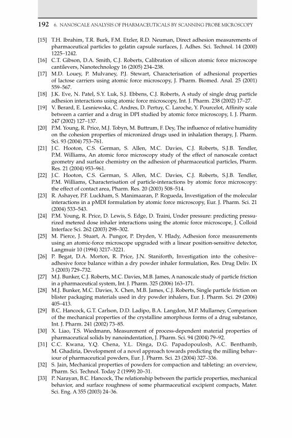
192 6. NANOSCALEANALySISOfPHARMACEUTICALSbySCANNINgPRObEMICROSCOPy
[15] T.H. Ibrahim, T.R. Burk, F.M. Etzler, R.D. Neuman, Direct adhesion measurements of pharmaceutical particles to gelatin capsule surfaces, J. Adhes. Sci. Technol. 14 (2000) 1225–1242.
[16] C.T. Gibson, D.A. Smith, C.J. Roberts, Calibration of silicon atomic force microscope cantilevers, Nanotechnology 16 (2005) 234–238.
[17] M.D. Louey, P. Mulvaney, P.J. Stewart, Characterisation of adhesional properties of lactose carriers using atomic force microscopy, J. Pharm. Biomed. Anal. 25 (2001) 559–567.
[18] J.K. Eve, N. Patel, S.Y. Luk, S.J. Ebbens, C.J. Roberts, A study of single drug particle adhesion interactions using atomic force microscopy, Int. J. Pharm. 238 (2002) 17–27.
[19] V. Berard, E. Lesniewska, C. Andres, D. Pertuy, C. Laroche, Y. Pourcelot, Affinity scale between a carrier and a drug in DPI studied by atomic force microscopy, I. J. Pharm. 247 (2002) 127–137.
[20] P.M. Young, R. Price, M.J. Tobyn, M. Buttrum, F. Dey, The influence of relative humidity on the cohesion properties of micronized drugs used in inhalation therapy, J. Pharm. Sci. 93 (2004) 753–761.
[21] J.C. Hooton, C.S. German, S. Allen, M.C. Davies, C.J. Roberts, S.J.B. Tendler, P.M. Williams, An atomic force microscopy study of the effect of nanoscale contact geometry and surface chemistry on the adhesion of pharmaceutical particles, Pharm. Res. 21 (2004) 953–961.
[22] J.C. Hooton, C.S. German, S. Allen, M.C. Davies, C.J. Roberts, S.J.B. Tendler, P.M. Williams, Characterisation of particle-interactions by atomic force microscopy: the effect of contact area, Pharm. Res. 20 (2003) 508–514.
[23] R. Ashayer, P.F. Luckham, S. Manimaaran, P. Rogueda, Investigation of the molecular interactions in a pMDI formulation by atomic force microscopy, Eur. J. Pharm. Sci. 21 (2004) 533–543.
[24] P.M. Young, R. Price, D. Lewis, S. Edge, D. Traini, Under pressure: predicting pressu-rized metered dose inhaler interactions using the atomic force microscope, J. Colloid Interface Sci. 262 (2003) 298–302.
[25] M. Pierce, J. Stuart, A. Pungor, P. Dryden, V. Hlady, Adhesion force measurements using an atomic-force microscope upgraded with a linear position-sensitive detector, Langmuir 10 (1994) 3217–3221.
[26] P. Begat, D.A. Morton, R. Price, J.N. Staniforth, Investigation into the cohesive– adhesive force balance within a dry powder inhaler formulation, Res. Drug Deliv. IX 3 (2003) 729–732.
[27] M.J. Bunker, C.J. Roberts, M.C. Davies, M.B. James, A nanoscale study of particle friction in a pharmaceutical system, Int. J. Pharm. 325 (2006) 163–171.
[28] M.J. Bunker, M.C. Davies, X. Chen, M.B. James, C.J. Roberts, Single particle friction on blister packaging materials used in dry powder inhalers, Eur. J. Pharm. Sci. 29 (2006) 405–413.
[29] B.C. Hancock, G.T. Carlson, D.D. Ladipo, B.A. Langdon, M.P. Mullarney, Comparison of the mechanical properties of the crystalline amorphous forms of a drug substance, Int. J. Pharm. 241 (2002) 73–85.
[30] X. Liao, T.S. Wiedmann, Measurement of process-dependent material properties of pharmaceutical solids by nanoindentation, J. Pharm. Sci. 94 (2004) 79–92.
[31] C.C. Kwana, Y.Q. Chena, Y.L. Dinga, D.G. Papadopoulosb, A.C. Benthamb, M. Ghadiria, Development of a novel approach towards predicting the milling behav-iour of pharmaceutical powders, Eur. J. Pharm. Sci. 23 (2004) 327–336.
[32] S. Jain, Mechanical properties of powders for compaction and tableting: an overview, Pharm. Sci. Technol. Today 2 (1999) 20–31.
[33] P. Narayan, B.C. Hancock, The relationship between the particle properties, mechanical behavior, and surface roughness of some pharmaceutical excipient compacts, Mater. Sci. Eng. A 355 (2003) 24–36.
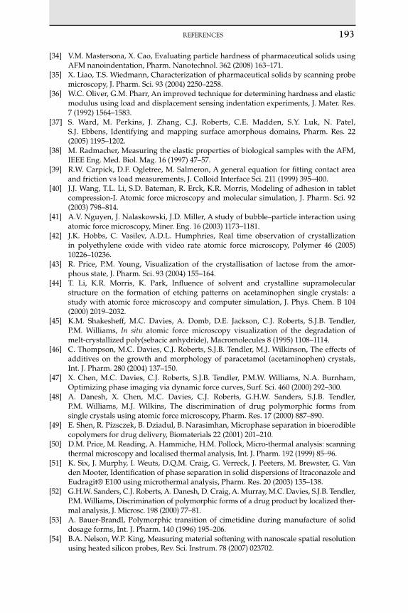
REfERENCES 193
[34] V.M. Mastersona, X. Cao, Evaluating particle hardness of pharmaceutical solids using AFM nanoindentation, Pharm. Nanotechnol. 362 (2008) 163–171.
[35] X. Liao, T.S. Wiedmann, Characterization of pharmaceutical solids by scanning probe microscopy, J. Pharm. Sci. 93 (2004) 2250–2258.
[36] W.C. Oliver, G.M. Pharr, An improved technique for determining hardness and elastic modulus using load and displacement sensing indentation experiments, J. Mater. Res. 7 (1992) 1564–1583.
[37] S. Ward, M. Perkins, J. Zhang, C.J. Roberts, C.E. Madden, S.Y. Luk, N. Patel, S.J. Ebbens, Identifying and mapping surface amorphous domains, Pharm. Res. 22 (2005) 1195–1202.
[38] M. Radmacher, Measuring the elastic properties of biological samples with the AFM, IEEE Eng. Med. Biol. Mag. 16 (1997) 47–57.
[39] R.W. Carpick, D.F. Ogletree, M. Salmeron, A general equation for fitting contact area and friction vs load measurements, J. Colloid Interface Sci. 211 (1999) 395–400.
[40] J.J. Wang, T.L. Li, S.D. Bateman, R. Erck, K.R. Morris, Modeling of adhesion in tablet compression-I. Atomic force microscopy and molecular simulation, J. Pharm. Sci. 92 (2003) 798–814.
[41] A.V. Nguyen, J. Nalaskowski, J.D. Miller, A study of bubble–particle interaction using atomic force microscopy, Miner. Eng. 16 (2003) 1173–1181.
[42] J.K. Hobbs, C. Vasilev, A.D.L. Humphries, Real time observation of crystallization in polyethylene oxide with video rate atomic force microscopy, Polymer 46 (2005) 10226–10236.
[43] R. Price, P.M. Young, Visualization of the crystallisation of lactose from the amor-phous state, J. Pharm. Sci. 93 (2004) 155–164.
[44] T. Li, K.R. Morris, K. Park, Influence of solvent and crystalline supramolecular structure on the formation of etching patterns on acetaminophen single crystals: a study with atomic force microscopy and computer simulation, J. Phys. Chem. B 104 (2000) 2019–2032.
[45] K.M. Shakesheff, M.C. Davies, A. Domb, D.E. Jackson, C.J. Roberts, S.J.B. Tendler, P.M. Williams, In situ atomic force microscopy visualization of the degradation of melt-crystallized poly(sebacic anhydride), Macromolecules 8 (1995) 1108–1114.
[46] C. Thompson, M.C. Davies, C.J. Roberts, S.J.B. Tendler, M.J. Wilkinson, The effects of additives on the growth and morphology of paracetamol (acetaminophen) crystals, Int. J. Pharm. 280 (2004) 137–150.
[47] X. Chen, M.C. Davies, C.J. Roberts, S.J.B. Tendler, P.M.W. Williams, N.A. Burnham, Optimizing phase imaging via dynamic force curves, Surf. Sci. 460 (2000) 292–300.
[48] A. Danesh, X. Chen, M.C. Davies, C.J. Roberts, G.H.W. Sanders, S.J.B. Tendler, P.M. Williams, M.J. Wilkins, The discrimination of drug polymorphic forms from single crystals using atomic force microscopy, Pharm. Res. 17 (2000) 887–890.
[49] E. Shen, R. Pizsczek, B. Dziadul, B. Narasimhan, Microphase separation in bioerodible copolymers for drug delivery, Biomaterials 22 (2001) 201–210.
[50] D.M. Price, M. Reading, A. Hammiche, H.M. Pollock, Micro-thermal analysis: scanning thermal microscopy and localised thermal analysis, Int. J. Pharm. 192 (1999) 85–96.
[51] K. Six, J. Murphy, I. Weuts, D.Q.M. Craig, G. Verreck, J. Peeters, M. Brewster, G. Van den Mooter, Identification of phase separation in solid dispersions of Itraconazole and Eudragit® E100 using microthermal analysis, Pharm. Res. 20 (2003) 135–138.
[52] G.H.W. Sanders, C.J. Roberts, A. Danesh, D. Craig, A. Murray, M.C. Davies, S.J.B. Tendler, P.M. Williams, Discrimination of polymorphic forms of a drug product by localized ther-mal analysis, J. Microsc. 198 (2000) 77–81.
[53] A. Bauer-Brandl, Polymorphic transition of cimetidine during manufacture of solid dosage forms, Int. J. Pharm. 140 (1996) 195–206.
[54] B.A. Nelson, W.P. King, Measuring material softening with nanoscale spatial resolution using heated silicon probes, Rev. Sci. Instrum. 78 (2007) 023702.

194 6. NANOSCALEANALySISOfPHARMACEUTICALSbySCANNINgPRObEMICROSCOPy
[55] P.G. Royall, V.L. Kett, C.S. Andrews, D.Q.M. Craig, Identification of crystalline and amorphous regions in low molecular weight materials using microthermal analysis, J. Phys. Chem. B 105 (2001) 7021–7026.
[56] L. Harding, W.P. King, X. Dail, D.Q.M. Craig, M. Reading, Nanoscale characterisation and imaging of partially amorphous materials using local thermomechanical analysis and heated tip AFM, Pharm. Res. 24 (2007) 2048–2054.
[57] T-H. Fang, W-J. Chang, Microthermal machining using scanning thermal microscopy, Appl. Surf. Sci. 240 (2005) 312–317.
[58] W.P. King, S. Saxena, B.A. Nelson, B.L. Weeks, R. Pitchimani, Nanoscale thermal anal-ysis of an energetic material, Nano Lett. 6 (2006) 2145–2149.
[59] L. Bond, S. Allen, M.C. Davies, C.J. Roberts, A.P. Shivji, S.J.B. Tendler, P.M. Williams, J. Zhang, Differential scanning calorimetry and scanning thermal microscopy analysis of pharmaceutical materials, Int. J. Pharm. 243 (2002) 71–82.

Atomic Force Microscopy in Process Engineering ©2009,ElsevierLtd195
O U T L I N E
7.1 Introduction 1957.1.1 How Do Cells Respond to the ECM? 196
7.2 Engineering the ECM for Probing Cell Sensing 1987.2.1 Surface Patterning (Chemical Signals) 1997.2.2 Nanotopography 2057.2.3 Nanoscale Measurement: Challenges and Opportunities for AFM 209
7.3 AFM in Cell Measurement 2117.3.1 AFM Imaging of Cells 2117.3.2 Elasticity Measurement of Living Cells 214
7.4 Conclusions 217
Acknowledgements 219
Abbreviations and Symbols 219References 220
Micro/NanoengineeringandAFMforCellularSensing
Huabing Yin, Gordon McPhee and Phil S. Dobson
7C H A P T E R
7.1 IntroduCtIon
Cells live in a complex extracellular matrix (ECM), which consists of neighbouring cells, proteins and extracellular fluids, inside the bodies of animals and plants. Cells constantly monitor the chemical and physical signals from their surroundings and react accordingly. A large body of

196 7. MICRO/NANOENgINEERINgANdAFMFORCELLULARSENSINg
evidence has shown that the various interactions between a cell and dif-ferent microenvironments play crucial roles in embryonic morphogenesis, tissue formation and maintenance of physiological functions [1]. Pertur-bations of cellular microenvironments or the adhesion of cells to the ECM can cause genetic defects, autoimmune diseases and cancers [2, 3]. It is also well known that in cancer metastasis, malignant cancer cells are able to break down tissue architecture and invade distant organ sites [4, 5].
The ECM is an intricate network within which biomolecules are precisely organised [6]. Classes of structural ECM proteins, mainly, col-lagen, glycoproteins and proteoglycans, form highly organised nanoscale structures, providing cells with both biological information and physical scaffolds for adhesion and migration. Although the regulatory functions of soluble factors (i.e. growth factors and hormones) present in the ECM have been well investigated, it has recently become increasingly recog-nised that the physics and mechanics of the ECM also have a significant impact on cell function and fate. Revealing the precise mechanisms under-lying these processes is intrinsically challenging – the events happen at many dimensions from single molecules to the macrotissue level, and in a dynamic/collective and hierarchical manner.
In order to better understand the interactions between the cells and the ECM and subsequent responses, engineered substrates and scaffolds are being developed to replace the native ECM. This has required inputs from many fields, ranging from surface engineering, material science and tissue engineering to cell biology. In this chapter, we will describe cur-rent developments of micro- and nanoengineered ECM materials and structures for the investigation of adhesion-associated responses of cells to chemical and mechanical cues. These efforts will be illustrated by an interconnected set of examples.
Importantly, as the length scales being examined in these studies have progressively shrunk, progress in interpreting the nanoworld has become increasingly dependent on techniques capable of nanoscale measurements within physiologically relevant environments. In this context, atomic force microscopy (AFM) has emerged as a powerful and multifunctional nanoscale tool, opening exciting new possibilities to address mechanistic questions in cell biology that may facilitate the development of efficient therapies for human health. In the following sections, we briefly intro-duce the basic biological principles for adhesion-associated cell sensing, followed by the engineering methods involved in generating substrates and materials to study cellular interactions, and finally the methodology associated with AFM measurements on these systems.
7.1.1 How do Cells respond to the ECM?
First, we review two important subcellular systems that are of funda-mental importance in cell adhesion to the ECM: the cell membrane and

7.1 INTROdUCTION 197
the cytoskeleton (Figure 7.1) (for background reading see, Alberts et al. [7]). The cell membrane is a barrier that separates the interior of the cell from the outside environment; it regulates the transport of molecules into and out of the cell and maintains the interior of the cell at optimal levels of pH and ionic concentrations. Cell membranes are primarily made of a selec-tively permeable lipid bilayer, containing various functional proteins that are involved in a range of specific cellular activities. For example, 25–50% of membrane receptors may be adhesive receptors [8]. The interior com-partment next to the cell membrane is the cytoplasm. This accommodates a number of specialised subcellular organelles that cooperate to maintain cell function. The cytoskeleton, which is located within the cytoplasm, is made up of three types of long rod-shaped molecules: microfilaments (e.g. actin stress fibre), microtubules (e.g. tubulin) and intermediate filaments (e.g. vimentin). These molecules attach to one another, link to other sub-cellular systems, such as the cell membrane and cell nucleus, and build a framework to give the cell both shape and movement. The configura-tion of the cytoskeleton dynamically adapts during cellular processes and undergoes microscopically observable morphological changes.
It is now clear that a particular family of transmembrane cell surface receptors, the integrins, mediate many of the interactions between a cell and the ECM. They both recognise peptide sequences, such as Arg-Gly-Asp (RGD) within the chains of certain ECM proteins (e.g. fibronectin), and connect the cytoskeleton to the ECM. During this process, adhesive contacts between the cell and the ECM are formed [9]. A common type of adhesive contact involves multiprotein complexes, called focal adhe-sions. These comprise integrins, the associated cytoplasmic proteins, and a number of protein kinases [1, 10]. Focal adhesions are the major sites for actin stress fibre attachment and thus a connection between the cytoskeleton and the ECM. Integrins that are bound to the ECM transmit
Direction of motion
Filopodium
PseudopodiumLamellopodium
ECM or substrate
MicrotubuleF-actin stress fibreFocal adhesion
Nucleus Cell membrane
FIgurE 7.1 Schematic drawing of cell adhesion to an ECM or substrate. The cell adheres firmly to the ECM through focal adhesions (a multiprotein complex). The focal adhesions are the sites for the attachment of F-actin stress fibres – one type of cytoskeleton protein. Filopodium and lamellopodium are located at the leading edge for cell to migrate.
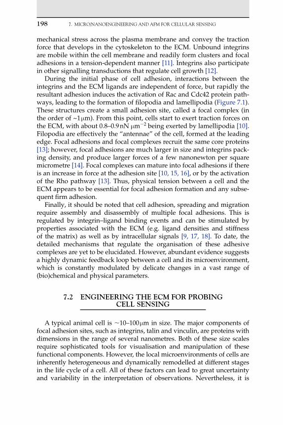
198 7. MICRO/NANOENgINEERINgANdAFMFORCELLULARSENSINg
mechanical stress across the plasma membrane and convey the traction force that develops in the cytoskeleton to the ECM. Unbound integrins are mobile within the cell membrane and readily form clusters and focal adhesions in a tension-dependent manner [11]. Integrins also participate in other signalling transductions that regulate cell growth [12].
During the initial phase of cell adhesion, interactions between the integrins and the ECM ligands are independent of force, but rapidly the resultant adhesion induces the activation of Rac and Cdc42 protein path-ways, leading to the formation of filopodia and lamellipodia (Figure 7.1). These structures create a small adhesion site, called a focal complex (in the order of ~1 m). From this point, cells start to exert traction forces on the ECM, with about 0.8–0.9 nN m2 being exerted by lamellipodia [10]. Filopodia are effectively the “antennae” of the cell, formed at the leading edge. Focal adhesions and focal complexes recruit the same core proteins [13]; however, focal adhesions are much larger in size and integrins pack-ing density, and produce larger forces of a few nanonewton per square micrometre [14]. Focal complexes can mature into focal adhesions if there is an increase in force at the adhesion site [10, 15, 16], or by the activation of the Rho pathway [13]. Thus, physical tension between a cell and the ECM appears to be essential for focal adhesion formation and any subse-quent firm adhesion.
Finally, it should be noted that cell adhesion, spreading and migration require assembly and disassembly of multiple focal adhesions. This is regulated by integrin–ligand binding events and can be stimulated by properties associated with the ECM (e.g. ligand densities and stiffness of the matrix) as well as by intracellular signals [9, 17, 18]. To date, the detailed mechanisms that regulate the organisation of these adhesive complexes are yet to be elucidated. However, abundant evidence suggests a highly dynamic feedback loop between a cell and its microenvironment, which is constantly modulated by delicate changes in a vast range of (bio)chemical and physical parameters.
7.2 EngInEErIng tHE ECM For ProbIng CEll SEnSIng
A typical animal cell is 10–100 m in size. The major components of focal adhesion sites, such as integrins, talin and vinculin, are proteins with dimensions in the range of several nanometres. Both of these size scales require sophisticated tools for visualisation and manipulation of these functional components. However, the local microenvironments of cells are inherently heterogeneous and dynamically remodelled at different stages in the life cycle of a cell. All of these factors can lead to great uncertainty and variability in the interpretation of observations. Nevertheless, it is

7.2 ENgINEERINgTHEECMFORPRObINgCELLSENSINg 199
because of these challenges that intense effort from many fields has been attracted, leading to the combination of micro- and nanotechnology with biological sciences and the formation of the interdisciplinary ‘bionano-technology’ field.
Advances in micro- and nanofabrication can produce precisely con-trolled model systems at a single molecule level, and provide a systematic approach to dissect the roles of intertwined parameters in the ECM. In combination with other approaches (including optical microscopy, AFM and scanning electron microscopy [SEM]), these fabrication methods have proven to be powerful in the elucidation of complex cell behaviour. Here we will discuss the development of engineered substrates for the investi-gation of cell interactions with the ECM. Specifically, we will review the achievements of these substrates in mimicking chemical and physical cues in the ECM. Although not explicitly stated in the review below, many of these studies described have been underpinned by AFM measurements of surface interactions, topography or materials compliance.
7.2.1 Surface Patterning (Chemical Signals)
MicropatterningMicropatterning is based on photolithography [19], which produces
features with dimensions over 1 m. As illustrated in the schematic rep-resentation in Figure 7.2(A), this process involves the UV irradiation of a spin-coated photosensitive polymer layer (photoresist) through a mask. UV irradiation through the mask causes the photoresist polymer chains to either break up (positive resist) or crosslink (negative resist), leading to a difference in solubility between the exposed and unexposed regions when immersed in a “developer” solution. After developing, the patterns from the mask have been effectively transferred onto the substrate. The patterned photoresist can then serve as a protecting layer in subsequent processes, such as lift-off to produce metal patterns, or etching to gener-ate a relief on the substrate.
Micropatterning has been extensively used for surface patterning of biological molecules. Its main purpose is to allow fine control over the size and spatial arrangement of regions that can be specifically functionalised for the attachment of ECM proteins. For this, selective immobilisation of adhesive molecules on the patterned area is required. It should be noted that preventing the physisorption of biomolecules (especially proteins) on both the patterned and non-patterned surfaces is equally important, as non-specifically adsorbed proteins could also serve as an adhesive region for cell attachment.
A key development in the generation of chemically patterned substrates has exploited the formation of self-assembly monolayers (SAM) from heterobifunctional organic molecules that bear specific functional groups

200 7. MICRO/NANOENgINEERINgANdAFMFORCELLULARSENSINg
Pho
tolit
hog
raph
y
(a)
(b)
(c)
(d)
Mask
Substrate
Photoresist
Etching Lift-off
Metal
(e) (g)
(h)(f)(A)
(B)
(a) (b) (c)
(f) (e) (d)
FIgurE 7.2 Schematic diagram of methods used in micropatterning. (A) Photolithogra-phy and (B) microcontact printing. In photolithography a mask with opaque and transparent features is brought into contact with a substrate coated with a photosensitive polymer (pho-toresist) (a and b). UV light is shone through the mask, exposing the polymer beneath the transparent regions of the mask (c). The mask is removed and the resist developed, remov-ing either the exposed or unexposed regions of the resist depending on the resist type (d). The resist layer can be used as a protective mask during a process to etch the unprotected regions of the substrate (e)–(f). Alternatively, metal can be evaporated onto the sample, remaining on the regions of exposed substrate after the resist has been dissolved in a ‘lift-off’ process (g)–(h). In microcontact printing, a topographically patterned stamp is ‘inked’ by contacting it with a sample coated with the desired chemical species (a)–(c). When the inked stamp is brought into contact with a clean substrate, the species are deposited on the surface in patterned regions dictated by the topography of the stamp (d)–(f).
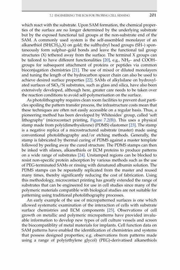
7.2 ENgINEERINgTHEECMFORPRObINgCELLSENSINg 201
which react with the substrate. Upon SAM formation, the chemical proper-ties of the surface are no longer determined by the underlying substrate but by the exposed functional tail groups at the non-substrate end of the SAM. A commonly used system is the self-assembled monolayer of an alkanethiol (SH(CH2)nX) on gold; the sulfhydryl head groups (SH–) spon-taneously form sulphur–gold bonds and leave the functional tail group structures (X) tethered away from the surface. The terminal X groups can be tailored to have different functionalities [20], e.g., NH2– and COOH– groups for subsequent attachment of proteins or peptides via common bioconjugation chemistries [21]. The use of mixed or diluted monolayers and tuning the length of the hydrocarbon spacer chain can also be used to achieve desired surface properties [22]. SAMs of alkylsilane on hydroxyl-ated surfaces of SiO2/Si substrates, such as glass and silica, have also been extensively developed, although here, greater care needs to be taken over the reaction conditions to avoid self-polymerisation on the surface.
As photolithography requires clean room facilities to prevent dust parti-cles spoiling the pattern transfer process, the infrastructure costs mean that these techniques are often not easily accessible on a regular basis. Thus, a pioneering method has been developed by Whitesides’ group, called ‘soft lithography’ (microcontact printing, Figure 7.2(B)). This uses a physical stamp made from poly(dimethysiloxne) (PDMS) elastomer [23]. The stamp is a negative replica of a microstructured substrate (master) made using conventional photolithography and/or etching methods. Generally, the stamp is fabricated by thermal curing of PDMS against a master template followed by peeling away the cured structure. The PDMS stamps can then be inked with silanes, alkanethiols or ECM proteins to produce patterns on a wide range of substrates [24]. Unstamped regions can be blocked to resist non-specific protein adsorption by various methods such as the use of PEG-terminated SAMs or rinsing with denatured albumin solution. The PDMS stamps can be repeatedly replicated from the master and reused many times, thereby significantly reducing the cost of fabrication. Using this methodology, microcontact printing has greatly extended the range of substrates that can be engineered for use in cell studies since many of the polymeric materials compatible with biological studies are not suitable for patterning using traditional photolithography processes.
An early example of the use of micropatterned surfaces is one which allowed systematic examination of the interaction of cells with substrate surface chemistries and ECM components [25]. Observations of cell growth on metallic and polymeric micropatterns have provided invalu-able information to develop new types of cell culture vessels and screen the biocompatiblity of metal materials for implants. Cell function data on SAM patterns have enabled the identification of chemistries and systems that possess designed properties; e.g. observations from patterns made using a range of poly(ethylene glycol) (PEG)-derivatised alkanethiols

202 7. MICRO/NANOENgINEERINgANdAFMFORCELLULARSENSINg
(and silanes) have found which exhibit the lowest protein physisorption (and hence block cell adhesion) [26–28]. These SAMs can therefore be used to form a non-adhesive background. By the integration of specific adhesion ligands into these patterns, defined spatial distribution of the ligands can be formed, as shown in Figure 7.3(a). Here, a pattern of fluo-rescently labelled fibronectin on a PEG-passivated surface was prepared by photolithography. Figure 7.3(b) demonstrates that fibroblasts specifi-cally attach and proliferate in the adhesive islands.
Cellular interactions in vivo are largely varied. Different types of cells are juxtaposed in the ECM and each secretes different cues at different times. Thus, cells are exposed to temporally spatially regulated concen-trations or dynamically changing gradients of adhesive cues (e.g. due to diffusion of soluble molecules emanating from particular cells). With surface engineering being able to tune spatial distances and pattern sizes, micropatterning provides a convenient way to study how cells sense the spatial distribution of adhesive cues. A study of cells on a micropat-tern of ECM ligands has discovered that the amount of integrin does not always determine cell life or death, but instead this is often indicated by the degree of cell spreading and its shape [29]. Surface patterning of dif-ferent ligands for two types of cells has also advanced the in vitro study
(a)
100 μm
(b)
200 μm
FIgurE 7.3 Example of surface patterning for the generation of adhesive protein pat-terns. (a) Fluorescence-labelled fibronectin patterns on a glass substrate generated using photolithography. (b) 3T3 fibroblast specifically attached and growing on the collagen pat-terns but not on the PEG surface between the patterns.

7.2 ENgINEERINgTHEECMFORPRObINgCELLSENSINg 203
of parenchymal cells such as hepatocytes (liver cells) which require het-erotypic interactions between non-parenchymal cells (e.g. fibroblast) to maintain their liver cell phenotype [30]. In this study, the microfabrication approach allowed researchers to specify independent variables, including the formation of a heterotypic interface and the ratio of cell populations at specific locations in their samples, something which was not possible using traditional random co-culture methods.
Although many of the above findings have been made possible with the aid of micropatterning, they have also indicated the desirability of further investigation at smaller length scales (100 nm) where most of the molecular mechanisms relevant to cell biology can be discovered. Thus, we describe relatively recent investigations that have used nanopatterned engineered surfaces in the next subsection.
NanopatterningTo generate nanopatterns, electron beam lithography (EBL) is nor-
mally used since the spatial resolution of photolithography is limited by the diffraction of light. Rather than using a mask, EBL uses a focused electron beam to directly write patterns onto an electron beam sensitive resist. Since this is a serial writing method, i.e. tracks are written segment by segment, this technique can require a significant amount of time to write a single large area pattern and is thus very expensive. However, in a development similar to the soft lithography described earlier, nanopattern structures can also be imprinted onto a solid polymeric substrate (nanoim-printing lithography [NIL]), greatly reducing the cost [31, 32]; Figure 7.4). By combining NIL with self-assembled monolayer techniques, protein nanopatterns of dimension 100 nm have been produced [33, 34]. The combined capability of NIL and EBL for the generation of arbitrary nano-patterns on a wide range of materials has also led to the discovery of cell response to nanotopography, as discussed in later sections.
Other methods for nanopatterning biological molecules include scan-ning probe lithography [35], self-assembly nanofabrication using block copolymer, and colloidal lithography [36]. A good review of these tech-niques is given by Gates et al. [37]. However, to generate a statistically meaningful cellular study, fine tailored adhesive nanopatterns have to cover a large area, preferably of the order of square centimetre. This imposes a big challenge for some of the serial writing methods, such as scan probe-associated lithography, although new developments in parallel writing using multiple tips might mitigate this barrier.
As an example of an extension of the self-assembled block copolymer technique, recently, Spatz’s group have developed the ‘micelle diblock copolymer lithography’. This allows precise control of space between RGD ligands at the length scale of 10–200 nm [38]. This strategy uses self-assembly of diblock polymer of polystyrene-block-poly(2-vinylpyridine)
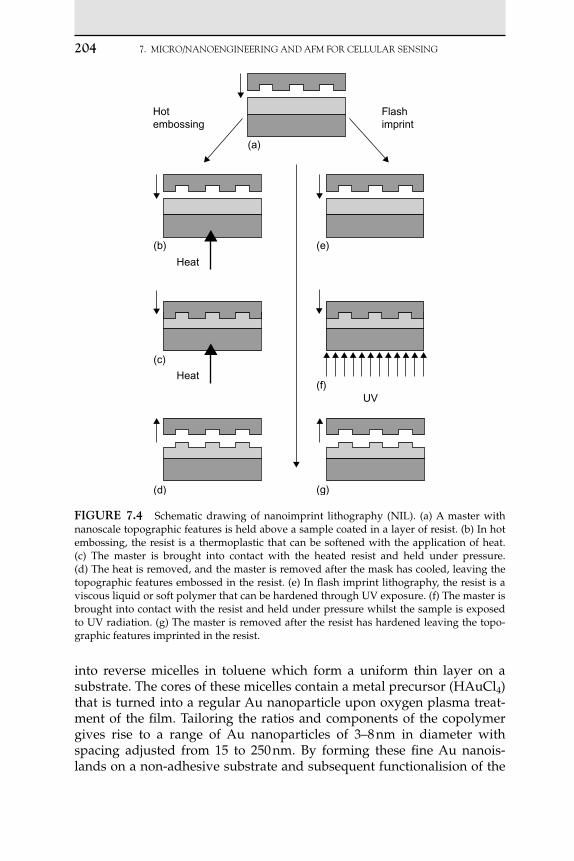
204 7. MICRO/NANOENgINEERINgANdAFMFORCELLULARSENSINg
into reverse micelles in toluene which form a uniform thin layer on a substrate. The cores of these micelles contain a metal precursor (HAuCl4) that is turned into a regular Au nanoparticle upon oxygen plasma treat-ment of the film. Tailoring the ratios and components of the copolymer gives rise to a range of Au nanoparticles of 3–8 nm in diameter with spacing adjusted from 15 to 250 nm. By forming these fine Au nanois-lands on a non-adhesive substrate and subsequent functionalision of the
Hotembossing
(a)
(b) (e)
(c)
(d)
(f)
(g)
Flashimprint
Heat
Heat
UV
FIgurE 7.4 Schematic drawing of nanoimprint lithography (NIL). (a) A master with nanoscale topographic features is held above a sample coated in a layer of resist. (b) In hot embossing, the resist is a thermoplastic that can be softened with the application of heat. (c) The master is brought into contact with the heated resist and held under pressure. (d) The heat is removed, and the master is removed after the mask has cooled, leaving the topographic features embossed in the resist. (e) In flash imprint lithography, the resist is a viscous liquid or soft polymer that can be hardened through UV exposure. (f) The master is brought into contact with the resist and held under pressure whilst the sample is exposed to UV radiation. (g) The master is removed after the resist has hardened leaving the topo-graphic features imprinted in the resist.

7.2 ENgINEERINgTHEECMFORPRObINgCELLSENSINg 205
Au nanoparticles with a cyclic RGD-thiol, nanoislands of RGD-ligands are created. This novel method has enabled a series of studies, demon-strating that cells can detect surface variations at the size of a typical pro-tein complex (100 nm) and are affected dramatically by small variations in ligand–cluster spacing (e.g. 58 and 73 nm) [39].
Although nanopatterning of adhesive molecules is ultimately valu-able to reveal molecular mechanisms underlying cellular processes, the reliability of the information obtained depends on the accuracy of the characterisation measurements at the nanoscale. In this context, it should be noted that topographic features as small as 10 nm can exert dramatic effects on a cell (more details in the next section). This type of observation is particularly important for protein nanopatterning studies based on the assembly of particle templates, as discussed in Spatz’s work.
7.2.2 nanotopography
In contrast to the use of micro- and nanoscale patterns of (bio)chemical motifs described earlier, cell behaviour has also been extensively stud-ied on patterns of micro- and nanoscale topographic features [40]. Motivation for many of these studies comes from the observation that although the physical form of the ECM appears as a random meshwork, in fact, it contains enormously detailed nano- and microscale structures. For instance, a corrugation with a period of 68 nm has been recently observed on collagen fibres [41]. When looked at on the small scale, the ECM possesses nanopores, micro- and nanofibres, and peaks and depres-sions. Since the middle of the twentieth century, it has been increasingly recognised that cells react to microtopography. Early evidence has shown that cells adhere, align and move along fibres in the range of 30–100 m [42–44]. In recent decades, the advance in micro- and nanofabrication has allowed intense investigations in this area and greatly push forward our understanding.
Since the early 1960s, Curtis and his colleagues have studied the reac-tion of a number of cell types with various microtopographic structures [40, 45]. Microgrooves with a wide combination of widths and depths have been studied, and it was found that cells react to both depth and width. In general, on deep and narrow grooves, cells tend to bridge between grooves, whilst on shallow grooves, they often follow the sur-face, although detailed reactions are cell type dependent [46]. Substantial evidence has been obtained, showing that adhesion or interaction with microscale topographic structures induces changes in cell cytoskeletal organisation, apoptosis (programmed cell death), macrophase activa-tion (causing inflammatory reactions) and gene expression [47, 48]. The observed phenomena clearly demonstrated that microtopography influ-ences cell development, and thus triggered researchers to pose questions

206 7. MICRO/NANOENgINEERINgANdAFMFORCELLULARSENSINg
about how cells sense the nanoworld, if indeed they can. For example, most of the commonly used cell culture dishes have a certain surface roughness, does this matter?
Random or Semi-Random Defined NanostructuresThe use of spontaneous phase separation of blended polymers or copo-
lymers provides an efficient way to produce different nanoscale features of controllable depths over a large area [49, 50]. By spin coating blends of polystyrene (PS) and poly(4-bromostyrene) (PBrS) onto silicon wafers and varying the ratio of polymers and their concentrations, nanoislands of heights between 13 and 95 nm were produced (Figure 7.5) and tested using fibroblast and endothelial cell cultures [51]. It was found that an enhanced cell response was observed on the nanostructured islands compared to the planar PS control: 13 nm height islands increased cell spreading and proliferation as well as a broad up-regulation of many genes involved in proliferation and matrix synthesis [52]. However, 95 nm high islands reduce cell spreading and proliferation [51]. Thus, by altering only the height of nanoscale features, a different cell response could be induced, demonstrating the significant roles that nanotopography might exert on cells.
Although polymer demixing can reliably control the z-depth of nanofea-tures, there can be less control over the lateral dimensions. In addition, for many systems a possible effect from the differences in the chemistry of two
FIgurE 7.5 AFM picture of an example of nanoislands made by polymer demixing process. Image courtesy of Drs. Matthew J. Dalby and Stanley Affrossman.

7.2 ENgINEERINgTHEECMFORPRObINgCELLSENSINg 207
polymers cannot be completely ruled out. Consequently, an alternative way for fast and low cost of fabrication of nanoscale topographic features has been sought through the use of colloidal lithography. Monodispersed and nanosized colloids made using wet chemistry techniques are commercially available. They can self-assemble into a monolayer on a substrate, with the spacing between each tailored by their surface charge or functional linker groups. The resulting colloid assembly is effectively a ‘photoresist’ pattern whose lateral dimensions are determined by the colloid size and spacing. Using this approach, nanocolumns of 160 nm height, 100 nm in diameter and 230 nm spacing have been produced in a bulk poly(methyl methacry-late) (PMMA) polymer [53, 54]. In comparison to the non-structured control, nanocolumns reduced focal adhesions of cells, but significantly increased density of filopodia formation. As discussed earlier, filopodia formation is associated with focal complexes, indicating the involvement of nanotopo-graphic features on integrin cluster formation.
The fact that many of the ECM proteins are present as nanofibres is driving intensive research on engineered nanofibres as replacements for ECM components. Carbon nanofibre compactions have been investigated for osteoblast culture with potential application as orthopedic/dental implants [55]. When compared with using conventional carbon fibres (diameter 100 nm), osteoblasts proliferate faster and deposit more extra-cellular calcium (indicating osteoblastic bone formation) on the carbon nanofibre compactions (diameter 100 nm). In other studies, synthetic and natural polymeric nanofibres have also long been regarded as prom-ising analogues of the ECM. Here, a vast selection of well-established methods can be used to tailor their chemistries to match those found in the native ECM. To produce the polymeric nanofibres themselves, electro-spining has become perhaps the simplest and most efficient technique for producing materials which can be assembled into 2D and 3D non-woven fibrous mesh (see review by Pham) [56]. Interestingly, cell culture on these nanofibre matrixes demonstrated better attachment and increased pro-liferation compared to that on substrates made from larger size fibres. Nanofibre meshes have also been found to stimulate cells to develop phenotypical behaviour [57, 58]. For example, NIH 3T3 fibroblasts and normal rat kidney cells grown on a polyamide nanofibre matrix displayed in vivo-like morphology and breast epithelial cells on the same matrix underwent morphogenesis into multicellular spheroids [58].
All the above-mentioned examples provide evidence which suggest that nanotopography has a significant influence on cell adhesion, cytoskeletal organisation and morphogenesis. However, the mechanisms involved are poorly understood: We do not know whether the less well-defined lateral dimensions of nanoislands made by either polymer mixing or colloidal lithography play any significant role in cellular behaviour; the nanofibre matrix may provide a large surface to volume ratio structure that could

208 7. MICRO/NANOENgINEERINgANdAFMFORCELLULARSENSINg
possibly entrap significant amounts of ECM proteins from the culture medium; and it is not clear as to what extent the chemistry and texture of the nanofibre matrix (or the nanoislands) interact with cells. As a random nanophase meshwork with poorly defined ‘nanotopography’ features, it is difficult to isolate the many parameters which might affect cells.
Precisely Defined NanostructuresE-beam lithography and associated techniques can produce precisely
defined nanostructures, so that individual variables can be investigated thoroughly. Features as small as 3 nm can be reliably fabricated on a sub-strate [59] and using modern high throughput machines, sufficiently large areas can be written for cellular studies. Through combination of EBL and NIL techniques, arbitrary nanopatterns can be replicated in thermo-plastic polymers. Using this method, a large number of replicates having identical patterns of designed nanofeatures have been produced on poly-lactide, polycarbonate, PMMA, and polycaprolactone [60–62]. This mass production using different materials has enabled direct comparison of the influence of substrates having different surface chemistries but the same nanotopography on cell behaviour for a number of cell lines.
The use of arbitrary nanopatterns provides a very flexible and system-atic way to explore the interactions between cells and the nanoworld, e.g. when highly regular arrays of nanopit structures with pit diameters of 35, 75 and 120 nm were used for fibroblast growth. Within this range of sub-tle variation in pit size, it was found that cell spreading reduced and there was less apparent stress fibre formation [60]. Following on from this study, EBL was used to create different levels of disorders in the nanopatterns. Using these levels it has been found that human mesenchymal stem cells (MSCs) were prompted to produce more bone mineral when there was a certain degree of disorder to the array patterns of nanopits (Figure 7.6; [61]). However, highly ordered nanopits resulted in low to negligible cel-lular adhesion and osteroblast differentiation. This discovery suggested that nanotopography might be an efficient method to guide MSC cells to be used in regenerative medicine and tissue engineering devices, since at present, many examples of failed bone implants have been found to be associated with encapsulation by soft tissue without direct bone bonding.
Clearly, substantial studies have advanced our understanding of the influence of topography on cellular processes. However, it is still to be resolved as to how cells detect and respond to these nanofeatures. Much evidence has shown that nanotopography influences cellular cytoskeleton formation, and thus is likely to modulate membrane receptor organisation, integrin cluster formation, and intracellular signalling – all of which are related to focal adhesion formation. It is not clear as to whether the mech-anosensitivity of cells to physical topography features employs the same machinery that cells use to sense changes in surface chemistry (e.g. adhe-sive patterns). New investigations have started to understand the changes
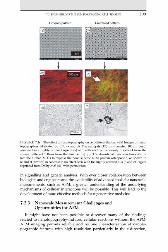
7.2 ENgINEERINgTHEECMFORPRObINgCELLSENSINg 209
in signalling and genetic analysis. With ever closer collaboration between biologists and engineers and the availability of advanced tools for nanoscale measurements, such as AFM, a greater understanding of the underlying mechanisms of cellular interactions will be possible. This will lead to the development of more effective methods for regenerative medicine.
7.2.3 nanoscale Measurement: Challenges and opportunities for AFM
It might have not been possible to discover many of the findings related to nanotopography-induced cellular reactions without the AFM. AFM imaging permits reliable and routine characterisation of nanoto-pographic features with high resolution particularly in the z-direction,
Ordered pattern
(a) (d)
(b) (e)
(c) (f)
200 μm
200 μm
1 μm
Disordered pattern
FIgurE 7.6 The effect of nanotopography on cell differentiation. SEM images of nano-topographies fabricated by EBL (a and d). The nanopits (120 nm diameter, 100 nm deep) arranged in a highly ordered square (a) and with each pit randomly displaced from the square pattern (50 nm from the true centre) (d). The disordered nanostructures stimu-late the human MSCs to express the bone-specific ECM protein osteopontin, as shown in (e and f) (arrows) in contrast to no effect seen with the highly ordered pits (b and c). Figure reprinted from Dalby et al. [61] with permission.

210 7. MICRO/NANOENgINEERINgANdAFMFORCELLULARSENSINg
facilitating the discovery of the significant effects on cell behaviour with subtle variations in the height of the nanoislands (13–95 nm) as described earlier (Figure 7.5). It has also long been desirable to image both nanoscale functional cellular components and nanostructures simultane-ously. In the past, biologists have employed SEM and immunostaining transmission electron microscopy (TEM) approaches to observe func-tional proteins (such as vinculin). However, these approaches require many steps of sample preparation, including cell fixing, immunostaining, sample drying, and thus many features can be disguised. Although AFM has been a powerful tool in the study of isolated biomolecular systems and their interactions, only more recently have nanoscale observations of living cells been achieved. The rapid expansion of the AFM approach to living cell studies has just started.
Many biological processes involve forces, and this is very much the case for cells adhering to the ECM. However, quantification of these forces is not straightforward, because a whole cell produces only small forces in the nanonewton range. Furthermore, the dimensions of functional com-ponents of a cell range from subnanometre (nucleic acid) to micrometre (whole cells), and measurements can be complicated by the whole cell structure dynamically remodelling during cell activities [14]. AFM with the ability to measure forces as small as piconewton and distances 1 nm demonstrates great flexibility and versatility for investigating the mechano- physical events occurring during biological interactions ranging from those of a single nucleic acid (deoxyribonucleic acid [DNA]) to those asso-ciated with whole intact cells.
AFM in conjunction with the colloidal probe techniques has further broadened its applications. Here, there are vast combinations in the choice, designs and functionalisation of probes, allowing a range of studies from a single biomolecular interaction to cell or polymer mechanics. The discov-ery that a cell exerts force on a substrate, as mentioned earlier, has initi-ated significant efforts to investigate the role of mechanical properties in cell activities. In this context, the AFM microsphere indentation technique has provided an assessment tool with high sensitivity and microscale res-olution that can perform well-defined investigations into cell interactions with substrates of different elasticity. In pioneering studies in this field it has been found that cell growth, differentiation, spreading and migration are all regulated by the elasticity of the substrates [63, 64].
As AFM is a surface-based technique with high resolution, the integra-tion of AFM with optical microscopes is essential for the investigation of intracellular events during scanning. There have been long standing ques-tions about the dynamics of structural adaptations of a cell in the context of mechanotransduction [65]. For example, how do cells use their cytoskel-eton conformation to transduce a mechanical stimulus to the nucleus and induce genomic variations? Frequently, there are also many requirements

7.3 AFMINCELLMEASUREMENT 211
for in situ monitoring of changes in intracellular signalling in combination with cellular physical variations as a result of the presence of drugs. These are most readily revealed by optical fluorescence assays. Consequently, in the last few years, instrument manufacturers have developed a number of combined AFM-optical microscope platforms that are now starting to benefit studies in the fields of bioengineering, cell engineering and basic cell biology. In particular, configurations involving confocal microscopy [66] and total internal reflection fluorescence microscopy [67] have already demonstrated their power in in situ living cell studies.
Since the invention of the AFM in 1986, we have witnessed significant growth of the employment of AFM to probe biological systems. In the next section we focus on recent developments associated with intact cell measurement.
7.3 AFM In CEll MEASurEMEnt
The unique advantages of AFM in cell measurement lie in its capabil-ity of being able to simultaneously (1) image cell topology under near-physiological conditions, (2) measure mechanical properties of living cells, and (3) monitor functional cellular components and intracellular processes in conjunction with optical microscopy. This section will dem-onstrate the great potential of AFM for investigating the interaction of cells with their environment.
7.3.1 AFM Imaging of Cells
In the early days of AFM imaging of cells, the main restriction was the limited scan size of the instruments [68], due to cells being relatively large structures. As soon as the first instruments with scan ranges of sev-eral micrometres were developed, they were deployed to image cells [69]. Today, modern bio-AFM instruments integrate an AFM platform onto the stage of a conventional inverted optical microscope, thus enabling easy positioning of AFM tip over a particular region of cells (Figure 7.7(a)). This development has been very useful in identifying regions of interest in cell morphology and where cells react to the microstructured substrate (Figure 7.7(b)). In addition, the optical imaging also permits simultane-ous monitoring of the lateral morphology of cells and/or intracellular signalling during the investigation by AFM [70]. Through a ‘direct over-lay’ technique, it is possible to integrate AFM with optical images and use the optical image to guide AFM operation. This enables correlation of the biophysical and biochemical functionalities of a cell. In reality, the dif-ferent operating principles of AFM and optical microscopy can result in

212 7. MICRO/NANOENgINEERINgANdAFMFORCELLULARSENSINg
an inaccurate overlay of the two images; however, this can be overcome by the use of registration methods devised by the manufacturers [71].
In many studies, fixed cells have been used to preserve cell morphol-ogy and maximise the imaging resolution with functional intracellular structures being revealed by staining. AFM and fluorescence images of an osteoblast cell cultured on a nanopatterned polycarbonate substrate prepared by EBL and NIL as described in an earlier section are shown in Figure 7.8. Although fluorescence images of the F-actin (light colour in Fig. 7.8(a)) and tubulin (light colour in Fig. 7.8(b)) elements within a cell protrusion already suggest a well-developed cytoskeleton structure, the AFM images reveal incredible details of the cell structure (Figure 7.8(c)–(f)). Both the well-spread straight actin stress fibres and the more curved tubulin network are visible. Here, the AFM image measures the height of the cell structures with a resolution that could not be obtained using techniques such as confocal microscopy. As is common practice with bio-logical cell measurements, AFM data are recorded in two image channels: the height image shows an overall topography and the error signal image highlights nanometre-scale surface topography, revealing well-defined variations in the structure. As a cautionary note, it should be noted that although the fixing procedure eases AFM imaging, it can also cause dam-age and alteration of delicate cellular structures [72].
Living cells, although more relevant to studies of most biological events, are one of the most challenging samples to image with AFM [73]. They are much softer than fixed cells and often react to the imaging process itself – sometimes retracting filopodia or excreting vesicles. Some cell types, e.g. fibroblasts are harder to image than others due to their restless nature
(a) (b)
FIgurE 7.7 Optical images of an AFM cantilever positioned over a cell on (a) a planar substrate and (b) a structured substrate.

7.3 AFMINCELLMEASUREMENT 213
under the tip, and the height contours of some are so steep as to prove difficult for the AFM tip to follow topographically. Thus, there are many considerations to take into account when designing experiments using live cell imaging, such as operation modes, loading force, choice of tip
(a) (b)
(e)
8
6183.3 nm
0 nm
4
2
0
Slo
w (μ
m)
0 2 4 6 8Fast (μm)
(f)
8
6129.7 mV
0 mV
4
2
0
Slo
w (μ
m)
0 2 4 6 8Fast (μm)
(c) (d)
40
20Slo
w (μ
m)
00 20
Fast (μm)
40
40645.5 nm
0 nm
309.1 nm
0 mV
20Slo
w (μ
m)
00 20
Fast (μm)
40
FIgurE 7.8 Simultaneous AFM and optical imaging of functional cell structures on a nanostructured substrate. Fluorescence images show an overview of the F-actin stress fibres (light colour in (a)) and tubulin (light colour in (b)) cytoskeleton protein distributed on a pro-trusion region (a and b). AFM height (c) and error images (d) revealing the detailed subcel-lular structures of the same region. The DirectoverlayTM feature (JPK instrument Ltd) was employed for image overlay and positioning of the AFM tip, permitting precise location of a zoomed in region (identified in d). AFM images (e and f) of the zoomed in region, revealing the filopodial interacting with the underlying nanopatterned structures. AFM imaging was carried out in contact mode using a silicon nitride cantilever with spring constant 0.01 N m1.

214 7. MICRO/NANOENgINEERINgANdAFMFORCELLULARSENSINg
and appropriate physiological conditions (medium temperature and pH). Although advances in cell immobilisation and AFM imaging modes now permit soft, live cells to be imaged, the process remains far from trivial [74].
For living cell imaging, an environmental control chamber with suit-able medium is essential to keep cells alive and viable. When imaging in contact mode, cantilevers with the lowest spring constants (0.003–0.06 N m1) operating with a small loading force (1 nN) are preferred. Following these basic considerations, it is possible to successfully image live cells. Figure 7.9(a)–(f) show height and error images of live 3T3 cells on a fibronectin-coated glass slide and a fibronectin-coated PDMS micro-grooved substrate. A well-spread cell morphology with fibrous cytoskel-eton structures can be seen clearly in Figure 7.9(a) in comparison to the restrained morphology of the cell on a flat PDMS substrate (Figure 7.9(c) and (d)). This can be further demonstrated by quantitative analysis of the cell height and its projecting area. It should be noted that cells tend to detach from the PDMS substrates during imaging. All of these observa-tions demonstrate that 3T3 fibroblasts have much weaker adhesion to soft PDMS substrates. On microstructured PDMS structures, cells tend to position their nucleus in the trough of the channel, close to one edge and mostly attach filopodia to the upper surfaces (Figure 7.9(e) and (f)). This gives rise to a preferred cell alignment along the channel length, as discussed earlier. Thus, AFM imaging provides a quantitative and high resolution approach to studying the behaviour of living cells.
7.3.2 Elasticity Measurement of living Cells
On a soft sample surface, an approaching tip with controlled force will cause an indentation. Although this is often problematic for AFM imag-ing of living cells, it is a way to measure and map the elastic properties of the cell structure. For a force–distance measurement, the deflection of the cantilever is plotted as function of the z-separation of the probe and the sample. On a stiff sample (e.g. glass), the deflection is proportional to the probe sample separation. However, on the soft sample, the move-ment of the tip will be less than that of the sample, and the difference is the indention of sample (Figure 7.10(a)).
In order to be able to extract material properties from an AFM force–distance curve, we must interpret the deflection using an appropriate model. As a starting point, it is reasonable to consider an AFM force– distance curve as arising from a conical tip indenting a planar surface. This was first considered by Hertz in 1882 [75] (equation (7.1)) and later generalised by Sneddon [76].
FE
v
π
22
2
1⋅ ⋅
( )⋅ ( )tan
(7.1)

7.3 AFMINCELLMEASUREMENT 215
This model has subsequently been applied to AFM data by many researchers [77, 78] and modified to account for a number of tip geom-etries [79]. In order to use the Hertz model to calculate the Young’s modulus (E) of a sample, several experimental parameters have to be known: the applied force (F), indentation depth (), semi-opening
100
50
718 nm
0 nm
Slo
w [μ
m]
00 50
Fast [μm](a)
100
50
Slo
w [μ
m]
00 50
Fast [μm](b)
428.7 mV
0 mV
100
20
7.749 nm
0 μm
Slo
w [μ
m]
00 20 40
Fast [μm](e)
40
20
0
Slo
w [μ
m]
0 20 40
Fast [μm](f)
1.375 V
0 V
80
60
40
20
2.774 μm
0 μm
Slo
w [μ
m]
00 50
Fast [μm](c)
80
60
40
20
2.038 V
0 V
Slo
w [μ
m]
00 50
Fast [μm](d)
FIgurE 7.9 AFM images of living cells on different substrates, glass (a and b), flat PDMS (c and d) and a microgrooved PDMS substrate (e and f). The grooves in (e) and (f) have a 12.5 m period and are 1 m deep. All the substrates were coated with fibronectin.

216 7. MICRO/NANOENgINEERINgANdAFMFORCELLULARSENSINg
angle of the tip (, only for a conical tip) and Poisson’s ratio (v, nor-mally assumed to be 0.5 as cells are virtually incompressible). Young’s modulus can then be calculated by taking and F at a single point or by fitting to the contact region of a force distance (F–) curve. In the single-point method, a significant uncertainty comes from the accuracy of determining the point where the tip first contacts the surface with zero force (contact point). This can be extremely difficult, and so it is normally recommended to fit the data in the contact region.
δ
δ
δ + d
(a)
δ d
0.4
0.3
0.2
Forc
e (n
N)
0.1
Contact point
On glassOn nucleusOn filopodia
–1400 –1200 –1000 –800
Piezo-displacement (nm)
(b)
–600 –400 –200 0 2000.0
FIgurE 7.10 Schematic diagram showing indentation of a soft substrate by an AFM tip and cantilever (a). Contact point between the tip and substrate with no load or indentation of the sample (left image). Tip indenting the sample by a distance , with a load caused by the cantilever deflection d, the total displacement of the tip–sample separation is given by d (right image). Examples of force curves generated on a solid glass substrate (no inden-tation), a cell nucleus region and a filopodia region (b). Note the heterogeneity of the cell. The indentation distance into the sample () can be corrected by subtracting the cantilever deflection (d) from the piezo-displacement.
7.4 CONCLUSIONS 217
In using simple Hertz-based models, it is important to realise that they may be valid only for small indentations, in the region of 5–10% of the total sample depth. In the case of cells, this will result in the first 200–500 nm of indentation giving a valid fit, but at deeper indentations the underlying substrate will start to influence the data. To overcome this problem, there has been some work on models that can accommodate indentation deeper than 10% of the total sample thickness [80], although currently they are not as well established as the conventional Hertz model.
Other considerations that should be taken into account when measuring the mechanical properties of cells include the inhomogeneity and non-elas-tic nature of a cell. For example, the indentation of cell nucleus and filopo-dia is quite different as shown in Figure 7.10(b). Although it is assumed that the cell is truly elastic for the purpose of data analysis, some of the energy delivered during indentation will be dissipated due to the viscous and slightly plastic nature of a cell. This effect can be seen in the velocity- dependent hysteresis that can be observed in some experiments [78, 81]. Measurements may also vary between cells, or even on the same cell due to the internal components of cell moving beneath the indenting tip.
Since Tao et al. first utilised AFM for quantitative measurement of local elastic properties of a biological sample (cow tibia) [82], there has been significant growth in the use of AFM for elasticity measurements of liv-ing cells [83–86]. It has been found that the elasticity (or stiffness) of dif-ferent cell types can vary from 0.1 to 40 kPa [87], and cell elasticity might function as a quantitative indicator during cell differentiation. Many stud-ies have also shown that cancer cells are substantially softer than normal cells [88, 89], indicating that quantitative analysis of mechanical proper-ties could be used to differentiate between cancerous and normal cells with similar appearances. The quantitative information of local cell elas-ticity in nanoscale spatial resolution has also provided valuable insights into cellular processes such as cell spreading [90] and cell migration [91]. Monitoring the change in elasticity while treating cells with drugs that disrupt specific cytoskeletal structures (i.e. F-actin, tubulin and intermedi-ate filaments) reveals that the actin network mainly determines the elastic properties of living cells [66]. Apart from the continuous contribution to understanding fundamental cellular mechanisms, these developments are also promising for drug testing studies [92].
7.4 ConCluSIonS
Recent developments in micro- and nanoengineering have created many opportunities to investigate the complex processes in cellular biol-ogy. Engineered surfaces with micro- or nanoscale features, either chemical

218 7. MICRO/NANOENgINEERINgANdAFMFORCELLULARSENSINg
or physical in nature, have been reliably produced by various methods. Many of these structures have emerged from the novel combination of advances in micro- or nanofabrication, chemistry and biology. Surface patterning methods offer considerable flexibility in pattern design, ligand specificity and density, and surface composition to investigate interactions of cells with chemical variations in the ECM. A vast range of engineered topographic features, from micro- to nanoscale, have been found to play a significant regulatory role in cellular proliferation, migration and differen-tiation. These studies provide significant insights into mechanistic ques-tions of how cells are able to sense, integrate and respond to collective chemical and mechanical signals. In addition, they also demonstrate that engineered environments can regulate cell functions and fate, and thus open new opportunities of developing tailored biosubstrates for specific tissue cell types, although this is still at its early stage.
Optical microscopes and SEM have been essential tools for many of these studies; however, they are subject to many constraints in exploring the molecular mechanisms at subcellular or cellular level, which are essen-tial for the control of the biological pathway. AFM, having been estab-lished as an important tool in development of nanopatterned surfaces, has provided increased momentum to living system studies. Nanometre spatial imaging and quantitative measurement of mechanical proper-ties of functional components of a living cell have been reliably achieved. Long standing questions in the nanoworld, such as whether it is nanoscale topographic features or chemical patterns that predominate in induc-ing cellular reactions [40], may be answerable. The combination of AFM with existing optical techniques has already shown itself to be a powerful tool, and further insights will be gained into in vitro cell differentiation and disease diagnostics. Together with the engineered environments that can be employed to guide cell function and fate, it might be possible to move towards controlling biological pathways in cell culture, and so explore new medicines and therapies for human health.
There are still many open challenges in cell biology and in physiologi-cal and pathological dysfunctions. The convergence of micro- or nanoen-gineering, AFM and interfacial chemistry with cell biology tools might provide new opportunities to address these challenges. For example, a bet-ter understanding of the complex processes associated with a whole intact cell interacting with individual molecules when cells are in contact with a surface will facilitate the diagnostics of arthoroplastic failures and improve existing implants. A more ambitious approach is to regenerate failed tis-sue outside a body; this requires an engineered ECM with the functional-ities that are found in a body. Although there have been intensive efforts in these fields, researchers are still a long way from recreating an ECM with similar molecular architecture and functionalities of the ECM found in vivo.

AbbREvIATIONSANdSyMbOLS 219
Increasing collaborations between scientists and communities from various disciplines, including engineering, nanobiotechnology, materials, biology and clinical medicine, are essential to approach this goal.
ACknowlEdgEMEntS
H. Yin is supported by the Royal Society of Edinburgh as an RSE per-sonal research fellow. G. McPhee thanks the EPSRC for his studentship. P. S. Dobson is supported by an RCUK Academic Research Fellowship. We would like to thank Dr Matthew Dalby for proof reading and offering con-structive suggestions and samples. We also thank Drs Andrew Glide and Mathis Riehle and Professor Jon Cooper for their support and discussions.
AbbrEvIAtIonS And SyMbolS
Semi-opening angle of the tip °AFM Atomic force microscopeDNA Deoxyribonucleic acid, a nucleic acidE Young’s modulus N m2
EBL Electron beam lithographyECM Extracellular matrixF Applied force NMSCs Human mesenchymal stem cellsNIL Nanoimprinting lithographyPBrS Poly(4-bromostyrene)PDMS Poly(dimethysiloxne)PEG Poly(ethylene glycol)PMMA Poly(methyl methacrylate)PS PolystyreneRGD A peptide sequence consisting of
Arg-Gly-AspSAM Self-assembly monolayerSEM Scanning electron microscopyTEM Transmission electron microscopyV Poisson’s ratio, dimensionless Indentation depth m

220 7. MICRO/NANOENgINEERINgANdAFMFORCELLULARSENSINg
references [1] B.M. Gumbiner, Cell adhesion: the molecular basis of tissue architecture and morpho-
genesis, Cell 84 (3) (1996) 345–357. [2] K.P. Campbell, Muscular-dystrophies – loss of cytoskeleton extracellular-matrix linkage,
Cell 80 (5) (1995) 675–679. [3] A. Lukes, S. Mun-Bryce, M. Lukes, G.A. Rosenberg, Extracellular matrix degradation
by metalloproteinases and central nervous system diseases, Mol. Neurobiol. 19 (3) (1999) 267–284.
[4] R.H. Kramer, X.D. Shen, H. Zhou, Tumor cell invasion and survival in head and neck cancer, Cancer Metastasis Rev. 24 (1) (2005) 35–45.
[5] T. Demuth, M.E. Berens, Molecular mechanisms of glioma cell migration and invasion, J. Neurooncol. 70 (2) (2004) 217–228.
[6] M. Aumailley, B. Gayraud, Structure and biological activity of the extracellular matrix, J. Mol. Med. 76 (3–4) (1998) 253–265.
[7] B. Alberts, A. Johnson, P. Walter, J. Lewis, Molecular Biology of the Cell, Garland Science, Taylor & Francis Group, New York, 2008.
[8] A.N. Barclay, Concluding remarks and the challenge from the immune system, Faraday Discuss. (1998) 345–350.
[9] E. Ruoslahti, M.D. Pierschbacher, New perspectives in cell adhesion: RGD and integrins, Science 238 (4826) (1987) 491–497.
[10] C.G. Galbraith, K.M. Yamada, M.P. Sheetz, The relationship between force and focal complex development, J. Cell Biol. 159 (4) (2002) 695–705.
[11] D.A. Lauffenburger, A.F. Horwitz, Cell migration: a physically integrated molecular process, Cell 84 (3) (1996) 359–369.
[12] K. Burridge, M. ChrzanowskaWodnicka, Focal adhesions, contractility, and signaling, Annu. Rev. Cell Dev. Biol. 12 (1996) 463–518.
[13] K. Rottner, A. Hall, J.V. Small, Interplay between Rac and Rho in the control of substrate contact dynamics, Curr. Biol. 9 (12) (1999) 640–648.
[14] N.Q. Balaban, U.S. Schwarz, D. Riveline, P. Goichberg, G. Tzur, I. Sabanay, D. Mahalu, S. Safran, A. Bershadsky, L. Addadi, B. Geiger, Force and focal adhesion assembly: a close relationship studied using elastic micropatterned substrates, Nat. Cell Biol. 3 (5) (2001) 466–472.
[15] D. Riveline, E. Zamir, N.Q. Balaban, U.S. Schwarz, T. Ishizaki, S. Narumiya, Z. Kam, B. Geiger, A.D. Bershadsky, Focal contacts as mechanosensors: externally applied local mechanical force induces growth of focal contacts by an mDia1-dependent and ROCK-independent mechanism, J. Cell Biol. 153 (6) (2001) 1175–1185.
[16] N. Wang, J.P. Butler, D.E. Ingber, Mechanotransduction across the cell-surface and through the cytoskeleton, Science 260 (5111) (1993) 1124–1127.
[17] G. Maheshwari, G. Brown, D.A. Lauffenburger, A. Wells, L.G. Griffith, Cell adhe-sion and motility depend on nanoscale RGD clustering, J. Cell Sci. 113 (10) (2000) 1677–1686.
[18] C.Q. Lin, M.J. Bissell, Multifaceted regulation of cell – differentiation by extracellular-matrix, FASEB J. 7 (9) (1993) 737–743.
[19] M. Madou, Fundamentals of Microfabrication: The Science of Miniturization, CRC Press, Boca Raton, FL, 1998.
[20] C.D. Bain, J. Evall, G.M. Whitesides, Formation of monolayers by the coadsorption of thiols on gold – variation in the head group, tail group, and solvent, J. Am. Chem. Soc. 111 (18) (1989) 7155–7164.
[21] G.T. HermansonBioconjugate Techniques, Academic press, San Diego, 2002. [22] C.D. Bain, G.M. Whitesides, Formation of monolayers by the coadsorption of thiols
on gold – variation in the length of the alkyl chain, J. Am. Chem. Soc. 111 (18) (1989) 7164–7175.

REFERENCES 221
[23] Y.N. Xia, G.M. Whitesides, Soft lithography, Ann. Rev. Mater. Sci. 28 (1998) 153–184. [24] R.S. Kane, S. Takayama, E. Ostuni, D.E. Ingber, G.M. Whitesides, Patterning proteins
and cells using soft lithography, Biomaterials 20 (23–24) (1999) 2363–2376. [25] A. Folch, M. Toner, Microengineering of cellular interactions, Ann. Rev. Biomed. Eng.
2 (2000) 227–256. [26] K.L. Prime, G.M. Whitesides, Adsorption of proteins onto surfaces containing end –
attached oligo(ethylene oxide) – a model system using self-assembled monolayers, J. Am. Chem. Soc. 115 (23) (1993) 10714–10721.
[27] M. Mrksich, C.S. Chen, Y.N. Xia, L.E. Dike, D.E. Ingber, G.M. Whitesides, Controlling cell attachment on contoured surfaces with self-assembled monolayers of alkanethi-olates on gold, Proc. Nat. Acad. Sci. U.S.A. 93 (20) (1996) 10775–10778.
[28] E. Ostuni, R.G. Chapman, R.E. Holmlin, S. Takayama, G.M. Whitesides, A survey of structure–property relationships of surfaces that resist the adsorption of protein, Langmuir 17 (18) (2001) 5605–5620.
[29] C.S. Chen, M. Mrksich, S. Huang, G.M. Whitesides, D.E. Ingber, Geometric control of cell life and death, Science 276 (5317) (1997) 1425–1428.
[30] S.N. Bhatia, U.J. Balis, M.L. Yarmush, M. Toner, Effect of cell–cell interactions in pres-ervation of cellular phenotype: cocultivation of hepatocytes and nonparenchymal cells, FASEB J. 13 (14) (1999) 1883–1900.
[31] L.J. Guo, Nanoimprint lithography: methods and material requirements, Adv. Mater. 19 (4) (2007) 495–513.
[32] S.H. Ahn, L.J. Guo, High-speed roll-to-roll nanoimprint lithography on flexible plastic substrates, Adv. Mater. 20 (11) (2008) 2044–2049.
[33] D. Falconnet, D. Pasqui, S. Park, R. Eckert, H. Schift, J. Gobrecht, R. Barbucci, M. Textor, A novel approach to produce protein nanopatterns by combining nanoimprint lithogra-phy and molecular self-assembly, Nano Lett. 4 (10) (2004) 1909–1914.
[34] J.D. Hoff, L.J. Cheng, E. Meyhofer, L.J. Guo, A.J. Hunt, Nanoscale protein patterning by imprint lithography, Nano Lett. 4 (5) (2004) 853–857.
[35] R.D. Piner, J. Zhu, F. Xu, S.H. Hong, C.A. Mirkin, “Dip-pen” nanolithography, Science 283 (5402) (1999) 661–663.
[36] X.M. Li, J. Huskens, D.N. Reinhoudt, Reactive self-assembled monolayers on flat and nanoparticle surfaces, and their application in soft and scanning probe lithographic nanofabrication technologies, J. Mater. Chem. 14 (20) (2004) 2954–2971.
[37] B.D. Gates, Q.B. Xu, M. Stewart, D. Ryan, C.G. Willson, G.M. Whitesides, New approaches to nanofabrication: molding, printing, and other techniques, Chem. Rev. 105 (4) (2005) 1171–1196.
[38] P.P. Girard, E.A. Cavalcanti-Adam, R. Kemkemer, J.P. Spatz, Cellular chemomechanics at interfaces: sensing, integration and response, Soft Matter 3 (3) (2007) 307–326.
[39] M. Arnold, E.A. Cavalcanti-Adam, R. Glass, J. Blummel, W. Eck, M. Kantlehner, H. Kessler, J.P. Spatz, Activation of integrin function by nanopatterned adhesive inter-faces, Chemphyschem 5 (3) (2004) 383–388.
[40] A.S.G. Curtis, C.D. Wilkinson, Reactions of cells to topography, J. Biomater. Sci. Polym. Ed. 9 (12) (1998) 1313–1329.
[41] D. Meller, K. Peters, K. Meller, Human cornea and sclera studied by atomic force microscopy, Cell Tissue Res. 288 (1) (1997) 111–118.
[42] P. Weiss, Experiments on cell and axon orientation in vitro – the role of colloidal exu-dates in tissue organization, J. Exp. Zool. 100 (3) (1945) 353–386.
[43] P. Weiss, Cell Contact, Int. Rev. Cytol. Surv. Cell Biol. 7 (1958) 391–423. [44] P. Weiss, B. Garber, Shape and movement of mesenchyme cells as functions of the
physical structure of the medium – contributions to a quantitative morphology, Proc. Natl. Acad. Sci. U.S.A 38 (3) (1952) 264–280.
[45] A.S.G. Curtis, M. Varde, Control of cell behavior – topological factors, J. Natl. Cancer Inst. 33 (1) (1964) 15.
222 7. MICRO/NANOENgINEERINgANdAFMFORCELLULARSENSINg
[46] A. Curtis, C. Wilkinson, Topographical control of cells, Biomaterials 18 (24) (1997) 1573–1583.
[47] P. Clark, P. Connolly, A.S.G. Curtis, J.A.T. Dow, C.D.W. Wilkinson, Topographical con-trol of cell behavior. 1. Simple step cues, Development 99 (3) (1987) 439–448.
[48] P. Clark, P. Connolly, A.S.G. Curtis, J.A.T. Dow, C.D.W. Wilkinson, Topographical con-trol of cell behavior. 2. Multiple grooved substrate, Development 108 (4) (1990) 635–644.
[49] S. Affrossman, G. Henn, S.A. Oneill, R.A. Pethrick, M. Stamm, Surface topography and composition of deuterated polystyrene–poly(bromostyrene) blends, Macromolecules 29 (14) (1996) 5010–5016.
[50] N. Gadegaard, M.J. Dalby, M.O. Riehle, A.S.G. Curtis, S. Affrossman, Tubes with controllable internal nanotopography, Adv. Mater. 16 (20) (2004) 1857–1860.
[51] M.J. Dalby, M.O. Riehle, H.J.H. Johnstone, S. Affrossman, A.S.G. Curtis, Polymer-demixed nanotopography: control of fibroblast spreading and proliferation, Tissue Eng. 8 (6) (2002) 1099–1108.
[52] M.J. Dalby, S.J. Yarwood, M.O. Riehle, H.J.H. Johnstone, S. Affrossman, A.S.G. Curtsi, Increasing fibroblast response to materials using nanotopography: morphological and genetic measurements of cell response to 13-nm-high polymer demixed islands, Exp. Cell Res. 276 (1) (2002) 1–9.
[53] M.J. Dalby, M.O. Riehle, D.S. Sutherland, H. Agheli, A.S.G. Curtis, Changes in fibro-blast morphology in response to nano-columns produced by colloidal lithography, Biomaterials 25 (23) (2004) 5415–5422.
[54] M.J. Dalby, M.O. Riehle, D.S. Sutherland, H. Agheli, A.S.G. Curtis, Fibroblast response to a controlled nanoenvironment produced by colloidal lithography, J. Biomed. Mater. Res. A 69A (2) (2004) 314–322.
[55] K.L. Elias, R.L. Price, T.J. Webster, Enhanced functions of osteoblasts on nanometer diameter carbon fibers, Biomaterials 23 (15) (2002) 3279–3287.
[56] Q.P. Pham, U. Sharma, A.G. Mikos, Electrospinning of polymeric nanofibers for tissue engineering applications: a review, Tissue Eng. 12 (5) (2006) 1197–1211.
[57] X.M. Mo, C.Y. Xu, M. Kotaki, S. Ramakrishna, Electrospun P(LLA-CL) nanofiber: a biomimetic extracellular matrix for smooth muscle cell and endothelial cell prolifera-tion, Biomaterials 25 (10) (2004) 1883–1890.
[58] M. Schindler, I. Ahmed, J. Kamal, A. Nur-E-Kamal, T.H. Grafe, H.Y. Chung, S. Meiners, A synthetic nanofibrillar matrix promotes in vivo-like organization and morphogenesis for cells in culture, Biomaterials 26 (28) (2005) 5624–5631.
[59] D.R.S. Cumming, S. Thoms, S.P. Beaumont, J.M.R. Weaver, Fabrication of 3 nm wires using 100 keV electron beam lithography and poly(methyl methacrylate) resist, Appl. Phys. Lett. 68 (3) (1996) 322–324.
[60] M.J. Dalby, N. Gadegaard, M.O. Riehle, C.D.W. Wilkinson, A.S.G. Curtis, Investigating filopodia sensing using arrays of defined nano-pits down to 35 nm diameter in size, Int. J. Biochem. Cell Biol. 36 (10) (2004) 2005–2015.
[61] M.J. Dalby, N. Gadegaard, R. Tare, A. Andar, M.O. Riehle, P. Herzyk, C.D.W. Wilkinson, R.O.C. Oreffo, The control of human mesenchymal cell differentiation using nanoscale symmetry and disorder, Nat. Mater. 6 (12) (2007) 997–1003.
[62] M.J. Dalby, M.J.P. Biggs, N. Gadegaard, G. Kalna, C.D.W. Wilkinson, A.S.G. Curtis, Nanotopographical stimulation of mechanotransduction and changes in interphase centromere positioning, J. Cell. Biochem. 100 (2) (2007) 326–338.
[63] T. Yeung, P.C. Georges, L.A. Flanagan, B. Marg, M. Ortiz, M. Funaki, N. Zahir, W.Y. Ming, V. Weaver, P.A. Janmey, Effects of substrate stiffness on cell morphology, cytoskeletal structure, and adhesion, Cell Motil. Cytoskeleton 60 (1) (2005) 24–34.
[64] A.J. Engler, S. Sen, H.L. Sweeney, D.E. Discher, Matrix elasticity directs stem cell line-age specification, Cell 126 (4) (2006) 677–689.
[65] D.E. Ingber, I. Tensegrity, Cell structure and hierarchical systems biology, J. Cell Sci. 116 (7) (2003) 1157–1173.

REFERENCES 223
[66] G.T. Charras, M.A. Horton, Single cell mechanotransduction and its modulation ana-lyzed by atomic force microscope indentation, Biophys. J. 82 (6) (2002) 2970–2981.
[67] A.B. Mathur, G.A. Truskey, W.M. Reichert, Atomic force and total internal reflec-tion fluorescence microscopy for the study of force transmission in endothelial cells, Biophys. J. 78 (4) (2000) 1725–1735.
[68] H.G. Hansma, J.H. Hoh, Biomolecular imaging with the atomic-force microscope, Ann. Rev. Biophys. Biomol. Struct. 23 (1994) 115–139.
[69] S.A.C. Gould, B. Drake, C.B. Prater, A.L. Weisenhorn, S. Manne, H.G. Hansma, P.K. Hansma, J. Massie, M. Longmire, V. Elings, B.D. Northern, B. Mukergee, C.M. Peterson, W. Stoeckenius, T.R. Albrecht, C.F. Quate, From atoms to integrated-circuit chips, blood-cells, and bacteria with the atomic force microscope, in: 4th International Conference on Scanning Tunneling Microscopy/Spectroscopy, Oarai, Japan, 1989.
[70] Y.R. Silberberg, A.E. Pelling, G.E. Yakubov, W.R. Crum, D.J. Hawkes, M.A. Horton, Mitochondrial displacements in response to nanomechanical forces, J. Mol. Recognit. 21 (1) (2008) 30–36.
[71] JPK. Application notes. Available from: http://www.jpk.com/index.2.html.[72] S.H. Doak, D. Rogers, B. Jones, L. Francis, R.S. Conlan, C. Wright, High-resolution
imaging using a novel atomic force microscope and confocal laser scanning micro-scope hybrid instrument: essential sample preparation aspects, Histochem. Cell Biol. 130 (5) (2008) 909–916.
[73] H.J. Butt, E.K. Wolff, S.A.C. Gould, B.D. Northern, C.M. Peterson, P.K. Hansma, Imaging cells with the atomic force microscope, J. Struct. Biol. 105 (1–3) (1990) 54–61.
[74] Y.F. Dufrene, Nanoscale exploration of microbial surfaces using the atomic force microscope, Future Microbiol. 1 (4) (2006) 387–396.
[75] H. Hertz, Uber die Beruhrug fester elastischer Korper, Journal fur die Reine und Angewandte Mathematik 92 (1882) 156–171.
[76] I.N. Sneddon, The relation between load and penetration in the axisymmetric boussi-nesq problem for a punch of arbitrary profile, Int. J. Eng. Sci. 3 (1) (1965) 47–57.
[77] M. Radmacher, Measuring the elastic properties of biological samples with the AFM, IEEE Eng. Med. Biol. Mag. 16 (2) (1997) 47–57.
[78] M.J. Rosenbluth, W.A. Lam, D.A. Fletcher, Force microscopy of nonadherent cells: a comparison of leukemia cell deformability, Biophys. J. 90 (8) (2006) 2994–3003.
[79] D.C. Lin, E.K. Dmitriadis, F. Horkay, Robust strategies for automated AFM force curve analysis-II: adhesion-influenced indentation of soft, elastic materials, J. Biomech. Eng. Trans. ASME 129 (6) (2007) 904–912.
[80] D.C. Lin, F. Horkay, Nanomechanics of polymer gels and biological tissues: a critical review of analytical approaches in the Hertzian regime and beyond, Soft Matter 4 (4) (2008) 669–682.
[81] Q.S. Li, G.Y.H. Lee, C.N. Ong, C.T. Lim, AFM indentation study of breast cancer cells, Biochem. Biophys. Res. Commun. 374 (4) (2008) 609–613.
[82] N.J. Tao, S.M. Lindsay, S. Lees, Measuring the microelastic properties of biological – material, Biophys. J. 63 (4) (1992) 1165–1169.
[83] J.H. Hoh, C.A. Schoenenberger, Surface-morphology and mechanical-properties of MDCK monolayers by atomic-force microscopy, J. Cell Sci. 107 (1994) 1105–1114.
[84] J.A. Dvorak, E. Nagao, Kinetic analysis of the mitotic cycle of living vertebrate cells by atomic force microscopy, Exp. Cell Res. 242 (1) (1998) 69–74.
[85] C. Rotsch, K. Jacobson, M. Radmacher, Dimensional and mechanical dynamics of active and stable edges in motile fibroblasts investigated by using atomic force micro-scopy, Proc. Natl. Acad. Sci. U.S.A. 96 (3) (1999) 921–926.
[86] H.J. Butt, B. Cappella, M. Kappl, Force measurements with the atomic force micro-scope: technique, interpretation and applications, Surf. Sci. Rep. 59 (1–6) (2005) 1–152.
[87] P.A. Janmey, C.A. McCulloch, Cell mechanics: integrating cell responses to mechanical stimuli, Ann. Rev. Biomed. Eng. 9 (2007) 1–34.

224 7. MICRO/NANOENgINEERINgANdAFMFORCELLULARSENSINg
[88] S.E. Cross, Y.S. Jin, J. Rao, J.K. Gimzewski, Nanomechanical analysis of cells from cancer patients, Nat. Nanotechnol. 2 (12) (2007) 780–783.
[89] S. Suresh, Biomechanics and biophysics of cancer cells, Acta Biomater. 3 (4) (2007) 413–438.
[90] L. Soon, F. Braet, J. Condeelis, Moving in the right direction – nanoimaging in cancer cell motility and metastasis, Microsc. Res. Tech. 70 (3) (2007) 252–257.
[91] A.A. Wagh, E. Roan, K.E. Chapman, L.P. Desai, D.A. Rendon, E.C. Eckstein, C.M. Waters, Localized elasticity measured in epithelial cells migrating at a wound edge using atomic force microscopy, Am. J. Physiol. Lung Cell. Mol. Physiol. 295 (1) (2008) L54–L60.
[92] H. Oberleithner, C. Riethmuller, T. Ludwig, M. Hausberg, H. Schillers, Aldosterone remodels human endothelium, in: E.K. Hoffman (ed) International Symposium Cell Volume Control in Health and Disease, Blackwell Publishing, Copenhagen, Denmark, 2005.

Atomic Force Microscopy in Process Engineering ©2009,ElsevierLtd225
O U T L I N E
8.1 Introduction 225
8.2 Basic Concepts 227
8.3 End-grafted Polymer Chains 229
8.4 Diblock Copolymers Adsorbed on Surfaces 236
8.5 Star-shaped Polymers Adsorbed on Surfaces 237
8.6 Conclusions 240
Acknowledgements 241
List of Abbreviations 242
List of Symbols 242References 242
AtomicForceMicroscopyandPolymersonSurfaces
Vasileios Koutsos
8C H A P T E R
8.1 IntroDuCtIon
The surfaces of materials are routinely modified with coatings to pro-tect them in hostile conditions and to functionalise them for a variety of purposes. Polymer coatings play an important role in such modifications. Polymer synthetic chemists are nowadays able to produce a huge num-ber of different macromolecules of controlled structure and composition (and consequently function) in large quantities and at a relatively low cost. Furthermore, polymers are usually processed readily and inexpensively.
226 8. ATOMICFORCEMICROSCOPyANdPOLyMERSONSURFACES
Ultrathin polymer coatings, in particular, play a crucial role in many processes, ranging from decoration and protection against a variety of degradation agents (corrosion/chemical) [1] to microfabrication method-ologies for microelectronics [2] and biomedical devices [3]. In all situa-tions, at the polymer-solid interface, there is a layer of polymer chains that are in direct contact with the solid surface. The coating can be so thin that it actually consists of just one mono-macromolecular layer, i.e. a monolayer of polymer chains that are all in contact with the solid sur-face. Such monolayers are typically some nanometres thick (the thick-ness is of the order of the typical size of one polymer chain). In many cases, the solid surface is not fully covered with polymer chains, and we have the formation of a submonolayer, the structure of which can range from a complete layer occasionally disrupted by some isolated holes to a solid surface only partially covered by some isolated polymer islands. Depending on the molecular interactions and the number of chains at the surface (surface coverage), there is a variety of different continuous, semi-continuous and discontinuous nanopatterns and nanostructures that can be formed.
Polymer monolayers and submonolayers on solid surfaces play an important role for many technological applications such as nanopattern-ing and surface modifications used in microelectronics [4], colloidal sta-bility and flocculation [5], polymer reinforcement with nanofillers [6, 7], non-fouling biosurfaces [8], biocompatibility of medical implants [9], separations [10], microfluidics [11], adhesion, lubrication and friction modification [12]. Of particular importance are recent developments in the direction of achieving smart responsive surfaces to various external stimuli using polymer monolayers and nanostructures [13–15].
The atomic force microscope (AFM) [16] provides a spatial and force resolution in the order of angstroms and tens of piconewtons, respec-tively; therefore, it is ideally suited to study the fine morphology and physico-chemical properties of materials at the nanometre scale, directly in real space. This is of particular importance in the field of polymer- modified material surfaces. The traditional surface techniques lack the lateral resolution at the nanometre scale, which is necessary in order to analyse laterally inhomogeneous monolayers and submonolayers of polymers, macromolecular-size clusters and polymer nanostructures or nanopatterns. Furthermore, the AFM can operate under liquid conditions, providing a direct look of polymers anchored on surfaces in various solvent conditions. In many cases, solution-based processing techniques (e.g. dip-coating, spin-coating, droplet-evaporation, spraying) are employed and consequently, direct measurements within a good solvent (for the polymer) are of particular importance. AFM investigations within liquids can reveal and elucidate the physico-chemical phenomena governing the polymer monolayer behaviour during formation and processing.

8.2 BASICCONCEPTS 227
Fur-thermore, in many cases, mainly within biotechnology applications, the functional use of the polymer monolayer is under liquid (e.g. aqueous) conditions and in these cases AFM provides the opportunity for direct, real-space and real-time monitoring of the polymer layer during its func-tional role. In any case, it has to be noted that AFM studies of dry polymer monolayers are more numerous since they are easier to implement. To some extent, they can provide important snapshots of polymeric behaviour in the solution and can elucidate many aspects of the polymer behaviour.
In this chapter, first, a concise and simplified version of the fundamen-tal physical ideas of how polymer chains behave when they are in close proximity to surfaces is presented; the following part is dedicated to the main objective of this chapter, which is to demonstrate the potential, ver-satility and flexibility of the AFM technique to probe in a direct manner the nanoscale structural and physical properties of polymer monolayers and submonolayers. To this end, we use some selected examples from our own AFM studies. We show that the structural regimes depend on many factors such as surface interactions, polymer molecular weight, surface density, solvent conditions, chemical composition and molecular architecture. The structural properties of these ultrathin polymer films have a profound effect on various chemomechanical properties of the modified surfaces.
In summary, we show in a direct manner the important role of the AFM as a very appropriate characterisation technique and tool for the investigation of materials surfaces that has been modified and processed by polymer monolayers and submonolayers.
8.2 BASIC ConCEPtS
A polymer chain can be attached on a surface by physical (e.g. van der Waals, electrostatic forces) and chemical (e.g. covalent) bonds. Its behav-iour depends strongly on the characteristics of the attachment such as the number and position of attachment points (e.g. anchoring by its end or attachment points along the backbone of the chain) and bond strength, with chemical bonds being usually stronger than any physical attractive forces and hydrogen bonds (which are ranked as of moderate strength). One has to note that a large number of weak physical bonds can be a very efficient way of attachment and in this way a polymer chain can take a flat conformation (Figure 8.1). Nevertheless, the adsorption by chemical bonds (chemisorption) is considered irreversible, while adsorption by physical attractive forces (physisorption) is usually reversible under cer-tain processing conditions.
A polymer chain in good solvent conditions (e.g. polystyrene in toluene) is swollen since the polymer segments repel each other because of the
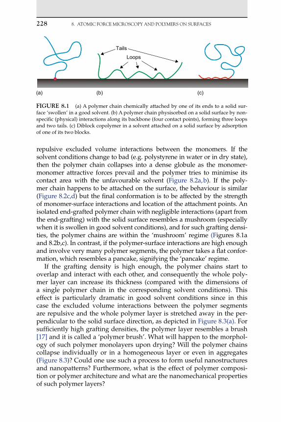
228 8. ATOMICFORCEMICROSCOPyANdPOLyMERSONSURFACES
repulsive excluded volume interactions between the monomers. If the solvent conditions change to bad (e.g. polystyrene in water or in dry state), then the polymer chain collapses into a dense globule as the monomer- monomer attractive forces prevail and the polymer tries to minimise its contact area with the unfavourable solvent (Figure 8.2a, b). If the poly-mer chain happens to be attached on the surface, the behaviour is similar (Figure 8.2c,d) but the final conformation is to be affected by the strength of monomer-surface interactions and location of the attachment points. An isolated end-grafted polymer chain with negligible interactions (apart from the end-grafting) with the solid surface resembles a mushroom (especially when it is swollen in good solvent conditions), and for such grafting densi-ties, the polymer chains are within the ‘mushroom’ regime (Figures 8.1a and 8.2b,c). In contrast, if the polymer-surface interactions are high enough and involve very many polymer segments, the polymer takes a flat confor-mation, which resembles a pancake, signifying the ‘pancake’ regime.
If the grafting density is high enough, the polymer chains start to overlap and interact with each other, and consequently the whole poly-mer layer can increase its thickness (compared with the dimensions of a single polymer chain in the corresponding solvent conditions). This effect is particularly dramatic in good solvent conditions since in this case the excluded volume interactions between the polymer segments are repulsive and the whole polymer layer is stretched away in the per-pendicular to the solid surface direction, as depicted in Figure 8.3(a). For sufficiently high grafting densities, the polymer layer resembles a brush [17] and it is called a ‘polymer brush’. What will happen to the morphol-ogy of such polymer monolayers upon drying? Will the polymer chains collapse individually or in a homogeneous layer or even in aggregates (Figure 8.3)? Could one use such a process to form useful nanostructures and nanopatterns? Furthermore, what is the effect of polymer composi-tion or polymer architecture and what are the nanomechanical properties of such polymer layers?
Tails
(a) (b) (c)
Loops
FIgurE 8.1 (a) A polymer chain chemically attached by one of its ends to a solid sur-face ‘swollen’ in a good solvent. (b) A polymer chain physisorbed on a solid surface by non-specific (physical) interactions along its backbone (four contact points), forming three loops and two tails. (c) Diblock copolymer in a solvent attached on a solid surface by adsorption of one of its two blocks.
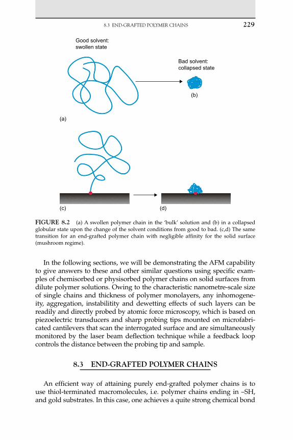
8.3 ENd-gRAFTEdPOLyMERCHAINS 229
In the following sections, we will be demonstrating the AFM capability to give answers to these and other similar questions using specific exam-ples of chemisorbed or physisorbed polymer chains on solid surfaces from dilute polymer solutions. Owing to the characteristic nanometre-scale size of single chains and thickness of polymer monolayers, any inhomogene-ity, aggregation, instabilitity and dewetting effects of such layers can be readily and directly probed by atomic force microscopy, which is based on piezoelectric transducers and sharp probing tips mounted on microfabri-cated cantilevers that scan the interrogated surface and are simultaneously monitored by the laser beam deflection technique while a feedback loop controls the distance between the probing tip and sample.
8.3 EnD-grAFtED PoLymEr ChAInS
An efficient way of attaining purely end-grafted polymer chains is to use thiol-terminated macromolecules, i.e. polymer chains ending in –SH, and gold substrates. In this case, one achieves a quite strong chemical bond
Good solvent:swollen state
Bad solvent:collapsed state
(a)
(c) (d)
(b)
FIgurE 8.2 (a) A swollen polymer chain in the ‘bulk’ solution and (b) in a collapsed globular state upon the change of the solvent conditions from good to bad. (c,d) The same transition for an end-grafted polymer chain with negligible affinity for the solid surface (mushroom regime).
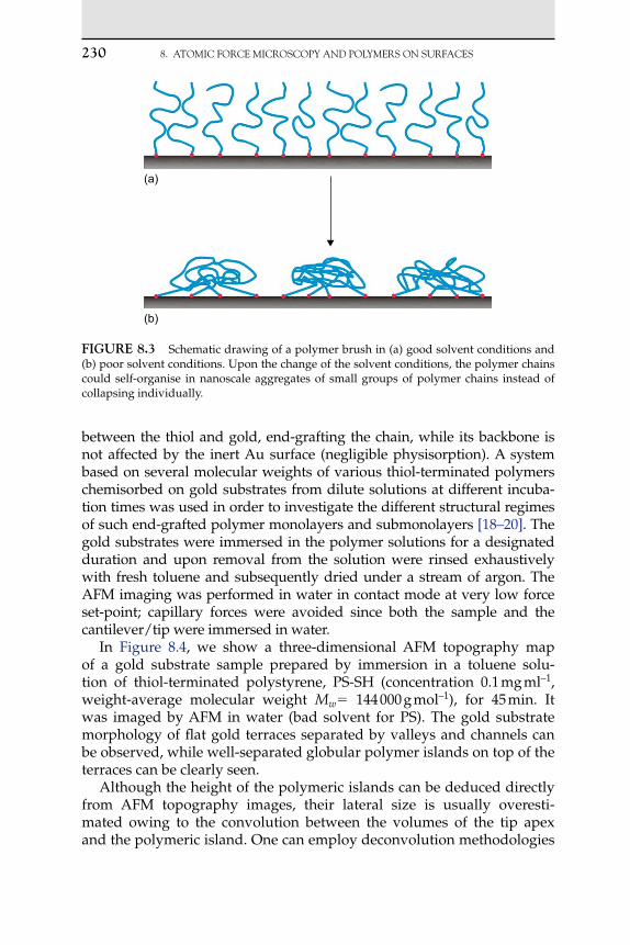
230 8. ATOMICFORCEMICROSCOPyANdPOLyMERSONSURFACES
between the thiol and gold, end-grafting the chain, while its backbone is not affected by the inert Au surface (negligible physisorption). A system based on several molecular weights of various thiol-terminated polymers chemisorbed on gold substrates from dilute solutions at different incuba-tion times was used in order to investigate the different structural regimes of such end-grafted polymer monolayers and submonolayers [18–20]. The gold substrates were immersed in the polymer solutions for a designated duration and upon removal from the solution were rinsed exhaustively with fresh toluene and subsequently dried under a stream of argon. The AFM imaging was performed in water in contact mode at very low force set-point; capillary forces were avoided since both the sample and the cantilever/tip were immersed in water.
In Figure 8.4, we show a three-dimensional AFM topography map of a gold substrate sample prepared by immersion in a toluene solu-tion of thiol-terminated polystyrene, PS-SH (concentration 0.1 mg ml–1, weight-average molecular weight Mw 144 000 g mol–1), for 45 min. It was imaged by AFM in water (bad solvent for PS). The gold substrate morphology of flat gold terraces separated by valleys and channels can be observed, while well-separated globular polymer islands on top of the terraces can be clearly seen.
Although the height of the polymeric islands can be deduced directly from AFM topography images, their lateral size is usually overesti- mated owing to the convolution between the volumes of the tip apex and the polymeric island. One can employ deconvolution methodologies
(a)
(b)
FIgurE 8.3 Schematic drawing of a polymer brush in (a) good solvent conditions and (b) poor solvent conditions. Upon the change of the solvent conditions, the polymer chains could self-organise in nanoscale aggregates of small groups of polymer chains instead of collapsing individually.

8.3 ENd-gRAFTEdPOLyMERCHAINS 231
including simple geometrical formulas in order to estimate the true volume of the islands [18, 20]. The dimensions of polymer islands deduced directly from AFM images show an average height and width of about 5.5 and 48 nm, respectively. As we have explained, although the mea-surement of height can be reliable, the width is usually overestimated owing to the convolution effect. Assuming that the shape of a polymer island is a spherical cap and taking into account the convolution effect, the average volume of the globules was estimated to be around 310 nm3. This compares well with the volume of a single collapsed polymer chain, which can be calculated assuming the usual bulk density for polystyrene (1 g cm–3). Therefore, we conclude that the polymer islands are isolated single polymer chains chemisorbed and collapsed into dense globules onto the gold substrate. This implies that for this incubation time the polymer chains are sparsely distributed and the grafting density is low enough for us to observe the ‘mushroom’ regime. The variation in the size of the polymer globules reflects the polymer polydispersity (Mw/Mn 1.2, where Mn is the number-average molecular weight) and possi-bly small changes in the globular conformation, which can be magnified by the convolution effect.
Figures 8.5 and 8.6 show two examples of gold substrates that were immersed in a toluene solution of higher concentration of PS-SH (2 mg ml–1) for much longer incubation times (2 days) and imaged under water in contact AFM mode. We can clearly see that the gold substrates are covered by a dense array of large polymer globules. Forty-eight hours is adequate time for the adsorption to reach its maximum grafting den-sity, and we expect to have several thousands of chains within a square
1000 nm
500 nm
0 nm 0 nm
500 nm
1000 nm
24.95 nm
FIgurE 8.4 AFM 3D-graph topography image of a gold substrate immersed in a toluene solution of PS-SH (concentration: 0.1 mg ml–1, molecular weight: 144 000 g mol–1) for 45 min. The AFM imaging was conducted in water, which is a bad solvent for PS. The polymer chains are in collapsed globular state and randomly distributed on the gold terraces.

232 8. ATOMICFORCEMICROSCOPyANdPOLyMERSONSURFACES
micrometre area. The globular islands are too many and too large in size to be individual collapsed chains.
Since for sufficiently long incubation time we expect to be close and above the overlap grafting density, the polymer chains are too close with each other to collapse separately. Instead, they collapse fusing together in small clusters, the size of which is moderated by the grafted tethers. They form aggregates connected to the surface through the tethers; these struc-tures have been called ‘pinned micelles’ or ‘octopus surface micelles’ and they have been predicted by theory [21, 22].
1000 nm
500 nm
0 nm 0 nm
500 nm
1000 nm
34.56 nm
FIgurE 8.5 AFM 3D-graph topography image of a gold substrate immersed in a tolu-ene solution of PS-SH (concentration: 2 mg ml–1, molecular weight: 258 000 g mol–1) for 48 h. The AFM imaging was conducted in water, which is a bad solvent for PS. The polymer chains form aggregates (pinned micelles) on the gold terraces.
1000 nm
500 nm
0 nm 0 nm
500 nm
1000 nm
29.25 nm
FIgurE 8.6 AFM 3D-graph topography image of a gold substrate immersed in a tolu-ene solution of PS-SH (concentration: 2 mg ml–1, molecular weight: 51 500 g mol–1) for 48 h. The AFM imaging was conducted in water, which is a bad solvent for PS. The polymer chains form aggregates (pinned micelles) on the gold terraces.

The polymeric islands can become more extended if the grafting den-sity is increased further. This can be attained by using a poorer solvent for the polymer solution; under poorer solvent conditions, the size of polymer chains is smaller and they can be chemisorbed much closer to each other. Figure 8.7 shows an AFM 3D-topography image of PS-SH chains end-grafted on the gold substrate from a cyclohexane (poor solvent for PS at room temperature) solution. In contrast with the well-separated polymer islands formed when the polymer monolayers were prepared in good solvent conditions, polymer monolayer formation under poor sol-vent conditions results in elongated and semi-continuous islands upon the evaporation of the solvent.
The lateral inhomogeneity manifested in polymer nanostructures and nanopatterns and clearly observed in our experiments is consistent with theory and simulations for end-grafted polymer chains at relatively high and uniform grafting densities [23–28]. It is to be expected that even higher grafting densities will result in a homogeneous layer upon the change of solvent conditions or drying of the solvent. However, such grafting densities are difficult to attain by a ‘grafting to’ technique like the one we employed owing to the steric hindrance of preadsorbed chains. Polymer brushes of very high grafting densities can be attained by ‘graft-ing from’ synthetic techniques, where the polymer chains grow from low–molecular weight initiators that are immobilized on the surface at very high density [17].
A polymer brush of uniform density in good solvent conditions forms a homogeneous layer that is stretched away from the surface owing to
8.3 ENd-gRAFTEdPOLyMERCHAINS 233
1000 nm
500 nm
0 nm0 nm 500 nm 1000 nm
0 nm
29 nm
FIgurE 8.7 AFM topography image of a collapsed PS-SH brush that was formed in poor solvent conditions (concentration: 0.1 mg ml–1, molecular weight: 144 000 g mol–1, incubation time: 1 h). The imaging has been performed in contact mode under water (bad solvent for PS).

234 8. ATOMICFORCEMICROSCOPyANdPOLyMERSONSURFACES
the repulsive excluded volume interactions between the polymer segments. The stretching of the chains is moderated by their entropic elasticity. Owing to the thermal agitation and fluctuations, a polymer chain adopts an overall shape that allows it to maximise the number of possible con-formations. Stretching decreases this number, which leads to an entropy loss, and for this reason a restoring force of entropic origin develops that resists deformation. A polymer brush in good solvent conditions should behave like a compliant/soft (non-linear) spring resisting compression, protecting the surface and even exhibiting low adhesive and frictional forces. An atomic force microscope allows us to probe directly the rele-vant nanomechanical properties at the local level.
We prepared a polymer brush system by immersing gold substrates to a dilute aqueous thiol-terminated poly(methacrylic acid), PMAA-SH, solu-tion for 24 h (Mw 66 200 g mol–1, Mw/Mn 2). We used AFM force spectros-copy (forward and reverse force distance curves) in deionised water (good solvent for PMAA) and acquired many force distance profiles. Two types of force profiles were observed on these monolayers. Figure 8.8(a) shows an example of the first type. During the forward movement of the tip towards the surface (approach), we observe the gradual increasing of the loading force owing to the non-linear compressive elasticity of the brush. No adhe-sive force is observed because the brush steric repulsion force screens the interaction of the tip with the substrate (in the same way that polymer chains anchored on colloidal particles stabilise their suspensions). During the reverse movement, there is no adhesion and the polymer brush is decompressed in a largely reversible way. Figure 8.8(b) shows that a simple exponential does describe the AFM data in the regime of intermedi-ate compression of the brush.
The Alexander–de Gennes theory of a polymer brush [29–31] predicts a certain relationship for its compression that can be approximated by the following exponential for intermediate compressions (0.2D/L00.9)
(b)D (nm)
100
10–1
10–2
F (
nN)
0 20 40 60 80 100
(a)
1.5
1.0
0.5
0.0
0 20 40 60
ForwardReverse
D (nm)
F (
nN)
80 100
FIgurE 8.8 (a) First type of force profile observed over a polymer brush. Notice the absence of hysteresis. (b) Logarithmic plot of the forward force distance curve.

8.3 ENd-gRAFTEdPOLyMERCHAINS 235
with a spherical probe: F(D) exp(2D/L0), where F(D) is the force exerted on the probe by the brush at a separation D between the probe surface and the solid substrate and L0 is the brush thickness.
We can directly check this equation on our data. We fitted several force profiles with the above equation and we obtained a brush thickness in the range of 100 nm, which is of the same order (albeit a bit larger) of the dis-tance D, where we observe in force profiles the initial increase of the force, signifying the extent (thickness) of the brush away from the surface. The discrepancy could arise from the fact that since our probe is small, a large proportion of the chains lie near the edge and therefore are expected to bend than to compress. A more appropriate theory must take into account the spherical shape of the tip and the lateral bending of the chains.
The second type of force profile is shown in Figure 8.9(a). The force profile during probe-tip approach is essentially the same: gradual increase of the loading force due to gradual compression of the brush. However, during the reverse force profile as the tip moves away from the surface, we observe some long-range attractive forces. The full length of one chain should be around 120 nm (calculated using the number-average molecu-lar weight Mn), which is consistent with the stretching events occurring up to approximately 200 nm. The magnitude of the attractive forces is in the range of 0.1–0.5 nN. Forces in this range can be attributed to physisorption of several monomers to a surface. Since we observe a gradual increase in the first derivative of these forces, we attribute them on parts of chains, individual chains and/or small clusters of chains that were adhered non-specifically to the tip and subsequently stretched during the reverse movement. The continuous lines in Figure 8.9 correspond to the entropic force for a single polymer chain using the freely jointed chain (FJC) model with full length approximately equal to the distance between the contact
(a) (b)
80
70
60
50
0.00 0.05 0.10 0.15
Non-linear elasticity
F (nN)
D (
nm)
1.5
1.0
0.5
0.0
–0.5
0 50 100 150
D (nm)
F (
nN) Theory
ForwardReverse
FIgurE 8.9 (a) Second type of force curve observed over a polymer brush. The con-tinuous lines correspond to the theoretical prediction for stretching of individual chains or parts of a chain. (b) Zoom of one of the long-range attractive force curves.
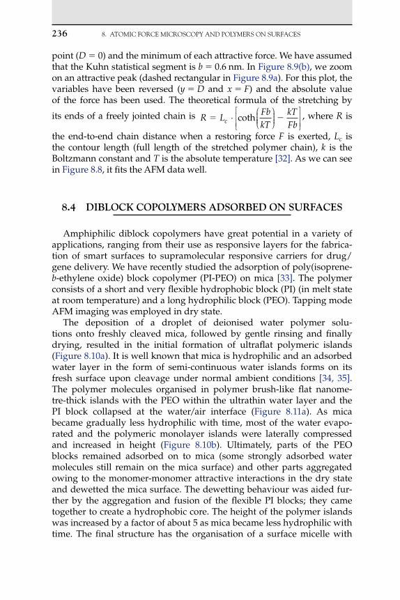
236 8. ATOMICFORCEMICROSCOPyANdPOLyMERSONSURFACES
point (D 0) and the minimum of each attractive force. We have assumed that the Kuhn statistical segment is b 0.6 nm. In Figure 8.9(b), we zoom on an attractive peak (dashed rectangular in Figure 8.9a). For this plot, the variables have been reversed (y D and x F) and the absolute value of the force has been used. The theoretical formula of the stretching by
its ends of a freely jointed chain is R LFbkT
kTFbc ⋅
coth , where R is
the end-to-end chain distance when a restoring force F is exerted, Lc is the contour length (full length of the stretched polymer chain), k is the Boltzmann constant and T is the absolute temperature [32]. As we can see in Figure 8.8, it fits the AFM data well.
8.4 DIBLoCk CoPoLymErS ADSorBED on SurFACES
Amphiphilic diblock copolymers have great potential in a variety of applications, ranging from their use as responsive layers for the fabrica-tion of smart surfaces to supramolecular responsive carriers for drug/gene delivery. We have recently studied the adsorption of poly(isoprene-b-ethylene oxide) block copolymer (PI-PEO) on mica [33]. The polymer consists of a short and very flexible hydrophobic block (PI) (in melt state at room temperature) and a long hydrophilic block (PEO). Tapping mode AFM imaging was employed in dry state.
The deposition of a droplet of deionised water polymer solu-tions onto freshly cleaved mica, followed by gentle rinsing and finally drying, resulted in the initial formation of ultraflat polymeric islands (Figure 8.10a). It is well known that mica is hydrophilic and an adsorbed water layer in the form of semi-continuous water islands forms on its fresh surface upon cleavage under normal ambient conditions [34, 35]. The polymer molecules organised in polymer brush-like flat nanome-tre-thick islands with the PEO within the ultrathin water layer and the PI block collapsed at the water/air interface (Figure 8.11a). As mica became gradually less hydrophilic with time, most of the water evapo-rated and the polymeric monolayer islands were laterally compressed and increased in height (Figure 8.10b). Ultimately, parts of the PEO blocks remained adsorbed on to mica (some strongly adsorbed water molecules still remain on the mica surface) and other parts aggregated owing to the monomer-monomer attractive interactions in the dry state and dewetted the mica surface. The dewetting behaviour was aided fur-ther by the aggregation and fusion of the flexible PI blocks; they came together to create a hydrophobic core. The height of the polymer islands was increased by a factor of about 5 as mica became less hydrophilic with time. The final structure has the organisation of a surface micelle with

8.5 STAR-SHAPEdPOLyMERSAdSORBEdONSURFACES 237
a hydrophobic core at the top and a stretched hydrophilic layer partially in close contact with the mica surface (Figures 8.10c and 8.11b).
8.5 StAr-ShAPED PoLymErS ADSorBED on SurFACES
Star-shaped polymers consist of several linear polymer chains (arms) covalently attached to a low–molecular weight core. They are of particu-lar interest in soft condensed matter since the number of arms (also called functionality) controls their interactions and consequently many physical properties. It is expected that as the number of arms increases, their polymer- like behaviour will change and become more colloidal-like.
We adsorbed polybutadiene (PB) star-shaped polymers of three differ-ent functionalities (number of arms: 18, 32 and 59) onto freshly cleaved mica surfaces from dilute polymer solutions in toluene. We investigated the structural regimes of the submonolayers and monolayers of adsorbed PB star polymers, which were formed on the mica surfaces by using AFM tapping mode imaging in dry state [36]. We attained various adsorbed
1000.0950.0
900.0850.0
800.0
Y [n
m]
X [nm]
Z [nm
]
750.0
700.0
650.0
5.02.0
0.0
–2300.0 –2200.0 –2100.0 –2000.0 –1900.0 –1800.0
(a) (b)
(c)
600.0
500.0
400.0
300.0
Y [n
m]
X [nm]
Z [nm
]
10.07.5
5.52.5
0.0
–2000.0 –1900.0 –1800.0 –1700.0 –1600.0 –1500.0 –1400.0
Y [n
m]
2600.0
2500.0
2400.0
2300.0
2200.0
Z [nm
]
0.02.5
5.07.5
10.0
12.5
15.0
17.5
20.0
X [nm]
–1800.0 –1700.0 –1600.0 –1500.0 –1400.0 –1300.0 –1200.0
FIgurE 8.10 AFM 3D-graph topography of a polymer island (a) 133 min, (b) 745 min and (c) 2980 min after sample preparation.

238 8. ATOMICFORCEMICROSCOPyANdPOLyMERSONSURFACES
amounts by employing several incubation times of the mica surface within the solution.
Figure 8.12 shows three examples of topographies of samples prepared using relatively short incubation times and consequently low adsorbed amounts. In this case, the polymer islands correspond to single and iso-lated polymer chains, as can be deduced by an analysis of their size from the AFM images. We can clearly see the asymmetric/irregular shape of the low-functionality star polymers and the gradual transition to more circular shapes as the functionality increased. Furthermore, the height of the individual star polymers increased with functionality; notice the flat ‘pancake’-like conformation taken by the low-functionality star polymers and the increased height of the high-functionality ones. It is clear that the higher the functionality, the closer is the star polymer behaviour to the one expected for a (soft) colloidal particle; their shape was affected much less strongly by the interactions with the surface.
Figure 8.13 shows an example of an image of sample prepared using incubation times in the solution long enough for the 18-arm star poly-mers to start interacting as they were swollen in good solvent conditions. Owing to the increased adsorbed amount, i.e. increased number of chains adsorbed on the surface, they compressed and confined each other, decreasing their lateral extension and simultaneously increasing their height. In this way, because of this confinement effect, they became uni-formly spaced, more symmetrical and circular in shape. At these moderate
Pl
Pl
PEO
PEO
(a)
(b)
FIgurE 8.11 Schematic drawing of the transition over time of the (a) initial brush-like flat polymer island to (b) a surface micelle. In (a), the PEO blocks are swollen and stretched away due to the presence of a water layer on mica surface and the resulting repulsive excluded volume interactions. In (b), most of water has evaporated and parts of the PEO blocks remain adsorbed on to the mica surface while other parts come together due to mon-omer-monomer attractions. The PI blocks fuse together in a compact core.

8.5 STAR-SHAPEdPOLyMERSAdSORBEdONSURFACES 239
adsorbed amounts, no interpenetration and fusion were observed. The star polymers continued to keep their individuality and they formed isolated globules upon the evaporation of the solvent.
In Figure 8.14, we compare the overall monolayer organisation for long incubation times. Such incubation times are long enough to achieve the maximum adsorbed amount (within our adsorption protocol using dilute polymer solutions). The 18-arm star polymers organised in discon-tinuous asymmetric islands, which consist of several individual polymer chains; it is clear that the star polymers penetrated each other when in good solvent and they collapsed in groups upon drying. The 32-arm star polymers also penetrated each other and they self-assembled in a con-tinuous dense network. On the other hand, the 59-arm star polymers did
X Range: 1.21 μm
Y R
ange
: 1.2
1μ
mHeight range: 2.234 nm
2
1.6
1.2
0.8
0.4
1.03 1.63 2.24
0.20
5–1
.00
–0.3
99
4
5
3
2
1
Height range: 5.050 nm
–1.26 –0.652 –0.0473
X Range: 1.21 μm
–0.5
60.
0452
0.65
Y R
ange
: 1.2
1μ
m
(b)
(c)
(a)
X Range: 1.21 μm
10
7.5
5
2.5
Height range: 10.03 nm
–2.3
2
–2.59 –1.98 –1.38
–1.7
1–1
.11
Y R
ange
: 1.2
1μ
m
FIgurE 8.12 AFM topography images of star polymers adsorbed on mica: (a) 18 arms, incubation time of 5 min; (b) 32 arms, incubation time of 10 min and (c) 59 arms, incubation time of 180 min.
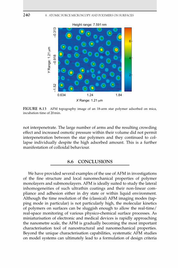
240 8. ATOMICFORCEMICROSCOPyANdPOLyMERSONSURFACES
not interpenetrate. The large number of arms and the resulting crowding effect and increased osmotic pressure within their volume did not permit interpenetration between the star polymers and they continued to col-lapse individually despite the high adsorbed amount. This is a further manifestation of colloidal behaviour.
8.6 ConCLuSIonS
We have provided several examples of the use of AFM in investigations of the fine structure and local nanomechanical properties of polymer monolayers and submonolayers. AFM is ideally suited to study the lateral inhomogeneities of such ultrathin coatings and their non-linear com-pliance and adhesion either in dry state or within liquid environment. Although the time resolution of the (classical) AFM imaging modes (tap-ping mode in particular) is not particularly high, the molecular kinetics of polymers on surfaces can be sluggish enough to allow the real-time/real-space monitoring of various physico-chemical surface processes. As miniaturisation of electronic and medical devices is rapidly approaching the nanometre scale, the AFM is gradually becoming the most important characterisation tool of nanostructural and nanomechanical properties. Beyond the unique characterisation capabilities, systematic AFM studies on model systems can ultimately lead to a formulation of design criteria
2
4
6
Height range: 7.591 nm
–0.3
13–0
.918
–1.5
2
0.634 1.24 1.84
Y R
ange
: 1.2
1μ
m
X Range: 1.21 μm
FIgurE 8.13 AFM topography image of an 18-arm star polymer adsorbed on mica, incubation time of 20 min.

ACkNOwLEdgEMENTS 241
for the processing of surfaces with polymers at the nanoscale for various engineering applications.
ACknowLEDgEmEntS
The author would like to thank all who have contributed to the research reviewed in this chapter, in particular Georges Hadziioannou (who also introduced me to this fascinating subject matter), Eric van der Vegte, Emmanouil Glynos, Stergios Pispas, Alexandros Chremos, Philip Camp, George Petekidis and Jacques Roovers.
Height range: 12.45 nm
10
7.5
5
2.5
X Range: 1.21 µm
–0.461
–1.1
4–0
.536
–0.0
684
0.144 0.749
Y R
ange
: 1.2
1 µm
(b)
(c)
(a)
Height range: 8.035 nm8
6
4
2
0.40
3–0
.201
–0.8
06
–0.67 –0.0649 0.54
X Range: 1.21 µm
Y R
ange
: 1.2
1µm
X Range: 1.22 µm
Z range: 4.352 nm
Y R
ange
: 1.2
2 µm
–0.9
76–1
.59
–2.2
0
0.341 0.953 1.56
1
2
3
4
FIgurE 8.14 AFM topography images of star polymers adsorbed on mica: (a) 18 arms, incubation time of 2880 min; (b) 32 arms, incubation time of 2440 min and (c) 59 arms, incu-bation time of 3600 min.
242 8. ATOMICFORCEMICROSCOPyANdPOLyMERSONSURFACES
LISt oF ABBrEvIAtIonS
AFM atomic force microscopeFJC freely jointed chainPB polybutadienePEO poly(ethylene oxide)PI polyisoprenePI-PEO poly(isoprene-b-ethylene oxide)PMAA poly(methacrylic acid)PMAA-SH thiol-terminated poly(methacrylic acid)PS polystyrenePS-SH thiol-terminated polystyrene–SH thiol
LISt oF SymBoLS
Unitb Kuhn statistical segment MD separation distance between the probe surface
and the solid substrate surfaceM
F force Nk Boltzmann’s constant (1.38 1023) J K1
Lc contour length of a polymer chain (full length of a stretched polymer chain)
M
L0 polymer brush thickness MMn number-average molecular weight g mol–1
Mw weight-average molecular weight g mol–1
R end-to-end polymer chain distance MT absolute temperature KX x-coordinate or abscissaY y-coordinate or ordinate
references [1] J.I.I. Laco, F.C. Villota, F.L. Mestres, Corrosion protection of carbon steel with thermo-
plastic coatings and alkyd resins containing polyaniline as conductive polymer, Prog. Org. Coat. 52 (2005) 151–160.

REFERENCES 243
[2] J.J. Licari, L.A. Hughes, Handbook of Polymer Coatings for Electronics: Chemistry, Technology and Applications Materials Science and Process Technology Series, second ed., Noyes Publications, New York, 1990.
[3] J. Lahann, Vapor-based polymer coatings for potential biomedical applications, Polym. Int. 55 (2006) 1361–1370.
[4] M.H. Jung, H. Lee, Patterning of conducting polymers using charged self-assembled monolayers, Langmuir 24 (2008) 9825–9831.
[5] M. Sjöberg, L. Bergström, A. Larsson, E. Sjöström, The effect of polymer and surfactant adsorption on the colloidal stability and rheology of kaolin dispersions, Colloids Surf. A Physicochem. Eng. Asp. 159 (1999) 197–208.
[6] Q.Q. Li, M. Zaiser, V. Koutsos, Carbon nanotube/epoxy resin composites using a block copolymer as a dispersing agent, Physica Status Solidi A Appl. Res. 201 (2004) R89–R91.
[7] M.J. Yang, V. Koutsos, M. Zaiser, Interactions between polymers and carbon nanotubes: a molecular dynamics study, J. Phys. Chem. B 109 (2005) 10009–10014.
[8] Z. Zhang, H. Vaisocherová, G. Cheng, W. Yang, H. Xue, S.Y. Jiang, Nonfouling behavior of polycarboxybetaine-grafted surfaces: structural and environmental effects, Biomacromolecules 9 (2008) 2686–2692.
[9] D. Pavithra, M. Doble, Biofilm formation, bacterial adhesion and host response on polymeric implants – issues and prevention, Biomed. Mater. 3 (2008) 034003.
[10] A. Kikuchi, T. Okano, Intelligent thermoresponsive polymeric stationary phases for aqueous chromatography of biological compounds, Prog. Polym. Sci. 27 (2002) 1165–1193.
[11] T. Rohr, D.F. Ogletree, F. Svec, J.M.J. Fréchet, Surface functionalization of thermoplastic polymers for the fabrication of microfluidic devices by photoinitiated grafting, Adv. Funct. Mater. 13 (2003) 264–270.
[12] L. Léger, E. Raphaël, H. Hervet, Surface-anchored polymer chains: their role in adhesion and friction, in: K. Binder and S. Granick (eds) Polymers in Confined Environments, Springer-Verlag, Berlin, 1999, pp. 185–225.
[13] S.H. Anastasiadis, H. Retsos, S. Pispas, N. Hadjichristidis, S. Neophytides, Smart polymer surfaces, Macromolecules 36 (2003) 1994–1999.
[14] C. Xu, X. Fu, M. Fryd, S. Xu, B.B. Wayland, K.I. Winey, R.J. Composto, Reversible stimuli- responsive nanostructures assembled from amphiphilic block copolymers, Nano Lett. 6 (2006) 282–287.
[15] P.M. Mendes, Stimuli-responsive surfaces for bio-applications, Chem. Soc. Rev. 37 (2008) 2512–2529.
[16] G. Binnig, C.F. Quate, C. Gerber, Atomic Force Microscope, Phys. Rev. Lett. 56 (1986) 930–933.
[17] B. Zhao, W.J. Brittain, Polymer brushes: surface-immobilized macromolecules, Prog. Polym. Sci. 25 (2000) 677–710.
[18] V. Koutsos, E.W. van der Vegte, P.C.M. Grim, G. Hadziioannou, Isolated polymer chains via mixed self-assembled monolayers: morphology and friction studied by scanning force microscopy, Macromolecules 31 (1998) 116–123.
[19] V. Koutsos, E.W. van der Vegte, G. Hadziioannou, Direct view of structural regimes of end-grafted polymer monolayers: a scanning force microscopy study, Macromolecules 32 (1999) 1233–1236.
[20] V. Koutsos, E.W. van der Vegte, E. Pelletier, A. Stamouli, G. Hadziioannou, Structure of chemically end-grafted polymer chains studied by scanning force microscopy in bad-solvent conditions, Macromolecules 30 (1997) 4719–4726.
[21] D.R.M. Williams, Grafted polymers in bad solvents – octopus surface micelles, Journal de Physique II 3 (1993) 1313–1318.
[22] E.B. Zhulina, T.M. Birshtein, V.A. Priamitsyn, L.I. Klushin, Inhomogeneous structure of collapsed polymer brushes under deformation, Macromolecules 28 (1995) 8612–8620.

244 8. ATOMICFORCEMICROSCOPyANdPOLyMERSONSURFACES
[23] P.Y. Lai, K. Binder, Structure and dynamics of polymer brushes near the theta point – a Monte-Carlo Simulation, J. Chem. Phys. 97 (1992) 586–595.
[24] G.S. Grest, M. Murat, Structure of grafted polymeric brushes in solvents of varying quality – a molecular-dynamics study, Macromolecules 26 (1993) 3108–3117.
[25] H. Tang, I. Szleifer, Phase-behavior of grafted polymers in poor solvents, Europhys. Lett. 28 (1994) 19–24.
[26] C. Yeung, A.C. Balazs, D. Jasnow, Lateral Instabilities in a grafted layer in a poor solvent, Macromolecules 26 (1993) 1914–1921.
[27] K.G. Soga, H. Guo, M.J. Zuckermann, Polymer brushes in a poor solvent, Europhys. Lett. 29 (1995) 531–536.
[28] R.S. Ross, P. Pincus, Bundles – end-grafted polymer layers in poor solvent, Europhys. Lett. 19 (1992) 79–84.
[29] S. Alexander, Adsorption of chain molecules with a polar head – a scaling description, Journal de Physique 38 (1977) 983–987.
[30] P.G. de Gennes, Conformations of polymers attached to an interface, Macromolecules 13 (1980) 1069–1075.
[31] P.G. de Gennes, Polymers at an interface – a simplified view, Adv. Colloid Interface Sci. 27 (1987) 189–209.
[32] A.Y. Grosberg, A.R. Khokhlov, Statistical physics of macromolecules, AIP Press, Woodbury, NY, 1994.
[33] E. Glynos, S. Pispas, V. Koutsos, Amphiphilic diblock copolymers on mica: formation of flat polymer nanoislands and evolution to protruding surface micelles, Macromolecules 41 (2008) 4313–4320.
[34] J. Hu, X.-d. Xiao, D.F. Ogletree, M. Salmeron, Imaging the condensation and evapora-tion of molecularly thin films of water with nanometer resolution, Science 268 (1995) 267–269.
[35] J. Hu, X.-d. Xiao, D.F. Ogletree, M. Salmeron, Structure of molecularly thin films of water on mica in humid environments, Surf. Sci. 344 (1995) 221–236.
[36] E. Glynos, A. Chremos, G. Petekidis, P.J. Camp, V. Koutsos, Polymer-like to soft colloid-like behavior of regular star polymers adsorbed on surfaces, Macromolecules 40 (2007) 6947–6958.
245
O U T L I N E
9.1 Introduction 245
9.2 Dynamic AFM Methods for the Characterisation of Material Properties 249
9.3 Dynamic Modulation Studies on Confined Fluids 252
9.4 Determination of Rheological Properties from Resonance Spectra 256
9.5 Cavitation and Adhesive Failure of Thin Films 259
9.6 Mesoscale Experimental Studies of the Tensile Behaviour of Thin Fluid Films 261
Acknowledgements 269
List of Symbols 269References 270
Application of Atomic Force Microscopy for
the Study of Tensile and Microrheological Properties
of FluidsMatthewS.BarrowandP.RhodriWilliams
9
9.1 InTRoDuCTIon
Atomic force microscopy is undeniably one of the most successful tech-niques for the characterisation of surfaces and is routinely used to describe structural details with nanoscale resolution [1]. The ability of atomic force
C H A P T E R

246 9. APPLICATION OF ATOMIC FORCE MICROSCOPy
microscopy to differentiate between local mechanical properties is well known, e.g. phase contrast maps obtained using tapping mode [2, 3] may be used to identify the distribution of components in composite materi-als. Alternatively, ‘adhesive’ forces may be determined by monitoring the deflection of a calibrated cantilever during contact and withdrawal of a probe from the surface of a ‘tacky’ material. During this process, the con-tact time and applied force may be varied, and by performing multiple tests at different locations, a representative ‘adhesive force map’ may be constructed. The atomic force microscope (AFM) is clearly a powerful tool for the investigation of forces which govern the mechanics of processes occurring at or below the microscale, and the exceptional ability of atomic force microscopy to determine forces associated with the microscale defor-mation and flow of fluids is presently discussed.
An understanding of the rheology of complex fluids is of fundamental importance in many practical engineering and biomedical applications. Traditional rheometrical techniques, e.g. cone and plate rheometers, require reasonably large volumes (i.e. several millilitres) of test fluid, which is often undesirable as limited volumes of fluid may be available, e.g. in studies of biological fluids. Many processes also involve the deformation of fluids in geometric confinement, which are not clearly described by the macroscale or bulk rheology alone, e.g. thin film lubrication, and in such instances, it is desirable to characterise the fluid mechanics under ostensibly similar conditions. Additionally, in such situations in situ measurement of fluid rheology is impaired by either the confined space or the extreme process environments.
The rheological behaviour of thin liquid films is an important aspect of lubrication [4] and printing [5] – processes which often involve meso-scale (0.110 m) thickness films undergoing rapid deformation between separating surfaces. In the case of fluid mechanical machinery, they are usually solid surfaces whereas in biomechanics they may be flexible surfaces such as biological membranes. The ‘cracking’ of knuckle joints has been attributed to cavitation within mesoscale lubricating films of syno-vial fluid [6] whereas surface damage in microelectromechanical systems devices has been attributed to the cavitation of lubricant films [7]. The ability of liquids to sustain tension is an important factor in the survival of plants in which the cohesion–tension (C–T) theory has been proposed to explain water transport [8]. The C–T theory assumes that water, when confined in small tubes with wettable walls such as xylem elements, can sustain a tension ranging from 3 to 30 MPa. The liquid forms a continuous system in the water-saturated cell walls from the evaporating surfaces of the leaves to the absorbing surfaces of the roots. During evaporation, the reduction in water potential at the surfaces causes movement of water out of the xylem, with water loss producing tension in the xylem sap that is transmitted throughout the continuous water columns to the roots.

In coating processes, cavitational film splitting may result in the for-mation of rapidly stretching filaments, whose breakup leads to unwanted droplet deposition. Filament formation is also a feature of coating flows involving adhesive films [9], but descriptions of the process are still largely qualitative, invoking terms such as ‘tack’ [10, 11]. The tack of an ink film is primarily connected with the tensile forces developed in film splitting [12], the function of cavitation being to limit the forces of sepa-ration of surfaces joined by a tacky liquid [13]. By definition, the tack of an ink film is the maximum tensile stress (or ‘negative pressure’) which can be withstood by it before splitting [5].
The subject area of micro- and nanorheology [14–18] has developed rapidly and benefited from the advent of the AFM and the surface force apparatus (SFA) [19, 20]. Roughly speaking, there are two principle objec-tives driving the development of AFM-based rheometrical techniques, the first considers the ability of AFM to describe the microrheological prop-erties of thin fluid films [21] whereas the second seeks to exploit AFM microcantilever technology as the basis for microsensor devices [22], which, e.g. may be incorporated into the so-called lab on a chip device. Specifically, it is envisaged that the development of MEMS devices such as diagnostic sensors incorporating microfluidic components can greatly benefit from an improved understanding of the microscale rheology.
In this respect, the determination of viscosity and density (or even simple representative damping coefficients) inferred via microflexural responses is of fundamental interest. This is because microcantilevers present a viable means by which the rheological properties of microvolumes of fluids may be assessed in situ. As an example, the resistive forces arising due to the motion of a cantilever within a minute volume of liquid can be analysed through changes in the cantilever response, as an immersed cantilever undergoing stimulated oscillation will experience fluid damping effects which are inter-rogable via resonance characteristics [23, 24]. Similarly, the ability to detect adsorbed mass (by monitoring changes in the resonance characteristics) in conjunction with functionalisation of the cantilever (or probe) surface repre-sents a potential approach to biomolecule or chemical species detection [25].
As the forces accompanying indentation or compression of a material by an AFM probe may be resolved with extreme accuracy, AFM-based techniques are particularly suited to rheological studies of predominantly elastic materials [26, 27]. In the simplest case, cantilever deflection may be used to describe the compliance of the surface in a simple qualitative manner, e.g. for a rigid, essentially undeformable material, the deflection of the cantilever will be equivalent to the downwards displacement of the piezoceramic actuator whereas for softer materials the probe will com-press and indent the sample such that the cantilever deflection is lower.
Probe–surface interactions assuming ideal elastic interactions are often used to determine the Young’s modulus of the material via derivatives of
9.1 INTROdUCTION 247

248 9. APPLICATION OF ATOMIC FORCE MICROSCOPy
the Hertz model (i.e. sphere against sphere compression) for non-adhesive systems. Furthermore, the Hertz model is readily adapted to provide idealised descriptions of geometries such as conical tips compressing flat substrates [28].
Notwithstanding the fact that AFM is routinely used in studies where elastic deformations are satisfactorily described by idealised models – a limitation of the use of AFM in many rheological experiments, particularly those involving fluids, is the assumed description of both the geometry and the flow field contained within.
Therefore, for the AFM-based study of fluids, the use of colloid probes [29] has proved to be of considerable benefit. Colloid probes (which are fabricated by attaching a colloid sphere to the underside of an AFM canti-lever) have found favour in several different research areas including the drainage of thin films [30], interfacial forces [31], mechanical properties of cells [32–34], lubrication theory [35] and the deformation of colloidal droplets [36, 37] to name but a few.
As has been alluded to previously, the successful use of AFM in microrheological and tribological studies is facilitated by the ability to describe force through the deflection and known spring constant of the cantilever. However, the topographical imaging capability of an AFM has been used as a component part of some studies. The imaging capabilities of an AFM have been used to measure the biaxial extensional deformation involved in the industrially important process of bubble inflation [38]. In this method the force-measuring capabilities of the AFM are not fully exploited, instead the AFM is used to measure the radius of curvature of microbubbles produced by inflating a thin polymer film, which is adhered to a porous silicon substrate. A similar approach is used to study the sur-face properties of polymers by using an AFM to measure the embedding rate of nanoparticles at temperatures near to the glass transition tempera-ture of the polymer [39].
Considering force measurement, one technique of particular relevance to tribology and lubrication studies is lateral force measurements in friction force microscopy (FFM) [40–44], which considers the torsion of a cantilever arising from frictional forces generated between a scanning tip and a sur-face. As lateral perturbations are caused by both frictional forces and surface features, it is informative to consider the local surface topography. The influ-ence of surface features upon the lateral deflection becomes apparent if the surface is scanned in opposing directions, as a topography-induced torsional response is dependent upon the scan direction (the torsion is reversed) whereas the lateral deflection arising from the effect of the frictional compo-nent will remain unchanged (Figure 9.1).
The beneficial application of microrheometry as an adjunct to tradi-tional bulk rheometry is demonstrated by the application of AFM force studies (including dynamic FFM, [45]) to adhesive materials. For example,

a combination of lateral force microscopy and indentation has been used to investigate the surface properties of pressure-sensitive adhesives (PSAs) [46], where the tack of the adhesive in response to various compressive loads is of paramount importance. Differences in local frictional forces due to increased adhesive force between the tip and the PSA arising from the incorporation of tack promoting components (tackifiers) may be identified. Therefore, FFM may be used to first identify microscale regions of vary-ing surface friction, following which the AFM can determine ‘adhesive’ characteristics of the different tackifier enriched or depleted regions. The correlation between traditional bulk tack and adhesion force as measured by AFM (or nanotack) is also considered by other workers [47], who find that the AFM force data are in general agreement with bulk tack tests.
9.2 DynAMIC AFM METhoDS FoR ThE ChARACTERISATIon oF MATERIAL PRoPERTIES
The nanorheological properties of polymeric liquids can be obtained by adapting techniques such as an SFA or an AFM to act in a dynamic mode [48, 49]. However, the results of AFM studies are often more difficult to interpret than those derived from SFA experiments due to uncertainties about the zero separation distance, the influence of probe asperities and torsional deflections.
Dynamic AFM, especially force modulation microscopy (FMM) [50–55], as a technique to determine the dominant elastic (and also viscoelastic) properties of materials has been investigated in many studies including the drainage of confined fluid layers [56], elastohydrodynamic lubrica-tion studies [57], approximations to the viscoelastic moduli of solvated polymer layers and the evaluation of temperature-induced variations in micromechanical properties [58]. Force modulation studies involve apply-ing a small amplitude (typically a few nanometres), sinusoidal oscillation
9.2 dyNAMIC AFM METHOdS 249
Scan direction
Friction forceCantilever
Tilt
FIguRE 9.1 FFM monitors the lateral deflection, i.e. tilt or ‘twist’ of the cantilever due to frictional resistance or drag forces in thin fluid layers acting upon the scanning tip.
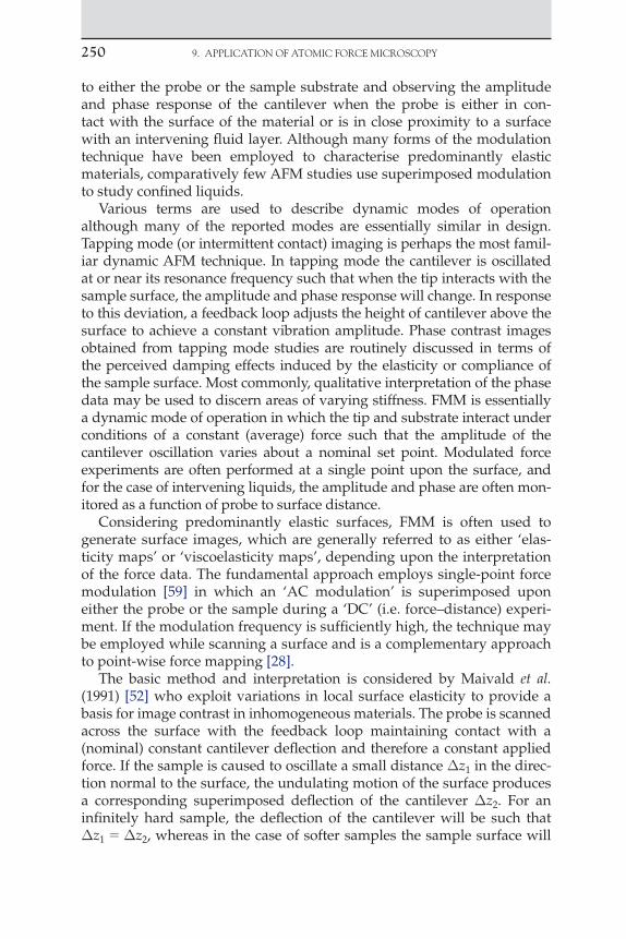
250 9. APPLICATION OF ATOMIC FORCE MICROSCOPy
to either the probe or the sample substrate and observing the amplitude and phase response of the cantilever when the probe is either in con-tact with the surface of the material or is in close proximity to a surface with an intervening fluid layer. Although many forms of the modulation technique have been employed to characterise predominantly elastic materials, comparatively few AFM studies use superimposed modulation to study confined liquids.
Various terms are used to describe dynamic modes of operation although many of the reported modes are essentially similar in design. Tapping mode (or intermittent contact) imaging is perhaps the most famil-iar dynamic AFM technique. In tapping mode the cantilever is oscillated at or near its resonance frequency such that when the tip interacts with the sample surface, the amplitude and phase response will change. In response to this deviation, a feedback loop adjusts the height of cantilever above the surface to achieve a constant vibration amplitude. Phase contrast images obtained from tapping mode studies are routinely discussed in terms of the perceived damping effects induced by the elasticity or compliance of the sample surface. Most commonly, qualitative interpretation of the phase data may be used to discern areas of varying stiffness. FMM is essentially a dynamic mode of operation in which the tip and substrate interact under conditions of a constant (average) force such that the amplitude of the cantilever oscillation varies about a nominal set point. Modulated force experiments are often performed at a single point upon the surface, and for the case of intervening liquids, the amplitude and phase are often mon-itored as a function of probe to surface distance.
Considering predominantly elastic surfaces, FMM is often used to generate surface images, which are generally referred to as either ‘elas-ticity maps’ or ‘viscoelasticity maps’, depending upon the interpretation of the force data. The fundamental approach employs single-point force modulation [59] in which an ‘AC modulation’ is superimposed upon either the probe or the sample during a ‘DC’ (i.e. force–distance) experi-ment. If the modulation frequency is sufficiently high, the technique may be employed while scanning a surface and is a complementary approach to point-wise force mapping [28].
The basic method and interpretation is considered by Maivald et al. (1991) [52] who exploit variations in local surface elasticity to provide a basis for image contrast in inhomogeneous materials. The probe is scanned across the surface with the feedback loop maintaining contact with a (nominal) constant cantilever deflection and therefore a constant applied force. If the sample is caused to oscillate a small distance z1 in the direc-tion normal to the surface, the undulating motion of the surface produces a corresponding superimposed deflection of the cantilever z2. For an infinitely hard sample, the deflection of the cantilever will be such that z1 z2, whereas in the case of softer samples the sample surface will

be compressed by a distance z3 such that z1 z2 z3. Therefore the deflection of the cantilever z2 is less on softer materials, and the term z2/z1 is deemed to be indicative of surface compliance (Figure 9.2).
This method can be implemented using the advanced capabilities of modern AFMs, one approach is similar to that described by Scott and Bushan (2003) [2]. In this example, the modulating amplitude is obtained by inducing vibration of the cantilever, the sample remaining fixed in posi-tion. Using an interleaved scanning approach, the sample height is first determined using tapping mode. The probe height is then adjusted such that (i) the probe is kept in constant contact with the surface and (ii) a con-stant scan height is maintained by compensating for the known sample height variation, i.e. the distance between the fixed end of the cantilever and the surface is held constant. The surface is then rescanned with the oscillating probe driven, in this case, at the resonant frequency (Figure 9.3).
Clearly, the method by which the sample–tip interaction is spatially modulated can be achieved in several ways. The probe may be caused
9.2 dyNAMIC AFM METHOdS 251
1 2
1 2
FIguRE 9.2 FMM: discrimination between areas of varying stiffness. (1) Hard substrate and (2) soft substrate; cantilever deflection signal z2 is reduced due to deformation of the sample.

252 9. APPLICATION OF ATOMIC FORCE MICROSCOPy
to oscillate by (i) the influence of an external driving force (such as a magnetic field), (ii) vibrating the sample using an electromechanical oscillator, (iii) mounting the cantilever on a secondary piezoceramic oscil-lator or (iv) modifying the primary piezoceramic scanner voltage. The preferred method may be influenced by the apparatus and the desired frequency range, as some oscillators exhibit mechanical resonances and produce excessive acoustic interference, the latter problem is likely to be more pronounced when the sample is contained in a small liquid cell. A wide range of modulation frequencies and experimental methods have been employed, ranging from a few hertz to several megahertz, and although the basic excitation principle is retained, the analytical meth-ods vary significantly. For example, atomic force acoustic microscopy (AFAM) employs excitation frequencies to several megahertz in order to elicit sample-specific, frequency-dependent spectra derived from contact measurements [60, 61].
9.3 DynAMIC MoDuLATIon STuDIES on ConFInED FLuIDS
For those studies where the viscoelastic response is of interest, attempts are made to relate the deflection amplitude and phase of the cantilever to the dynamic complex modulus G*() of the material. In standard rheometry, a sample subjected to a sinusoidally varying shear stress will respond with a sinusoidally varying shear strain, and the mechanical characteristics of the sample may then be described by the complex modulus as given by
G*( )
( )( )
ε
(9.1)
Surface profile from primary scan
FIguRE 9.3 Interleaved scanning wherein the force modulation scan uses the predeter-mined sample height.
where is the shear stress, ε the shear strain and the frequency. The complex modulus may be described as the summation of an in-phase elastic component and an out-of-phase viscous component, i.e.
G G i G*( ) ( ) ( ) ′ ′′ (9.2)
and
′′′
GG
( )( )
tan
(9.3)
where G is the storage (elastic) modulus, G″ the loss (viscous) modulus and the phase angle between stress and strain.
The analogy between bulk oscillatory and dynamic scanning probe microscope techniques is discussed by Suraya et al. (2008) [62], where for the latter, the motion of one surface imparts oscillatory motion to the fluid due to hydrodynamic forces, which in turn invokes oscillation of the ‘receiver’ surface, i.e. the colloid probe. However, although the receiver surface will oscillate at the same frequency, viscous effects are such that the oscillation amplitude is attenuated and the phase is shifted (relative to the driven surface). For an inelastic liquid, the detected signal will be 90° out-of-phase, whereas an elastic response is expected to be in-phase with the driven surface. When oscillating surfaces bearing adsorbed polymer layers are immersed in dilute polymer solutions, the vibrating motion produces a viscous response at large surface separations. As the separation distance is reduced, the polymer layers interact and deform, and the viscoelas-tic properties of the material become apparent as the receiver amplitude increases and the phase shift reduces.
Suraya et al. (2008) note that the measurement of the effect of the hydro-dynamic force upon the phase and amplitude is insufficient to directly measure the stress and strain in the fluid layer. To translate the measured parameters into terms which are physically representative of the stress and strain, a mechanical model is required. A common approach employs hydrodynamic lubrication equations, which conveniently describe the hydrodynamic force that arises from the flow of a purely viscous liquid between a flat surface and a colloid sphere, the force F is given by
F U
Rh
62
πη , ( )h R<<
(9.4)
where h is the separation distance, R the sphere radius and U is the rela-tive velocity of the surfaces. Equation (9.4) may also be applied to vis-coelastic fluids, where accordingly, the velocity, force and viscosity are described by complex quantities.
9.3 dyNAMIC MOdULATION STUdIES ON CONFINEd FLUIdS 253
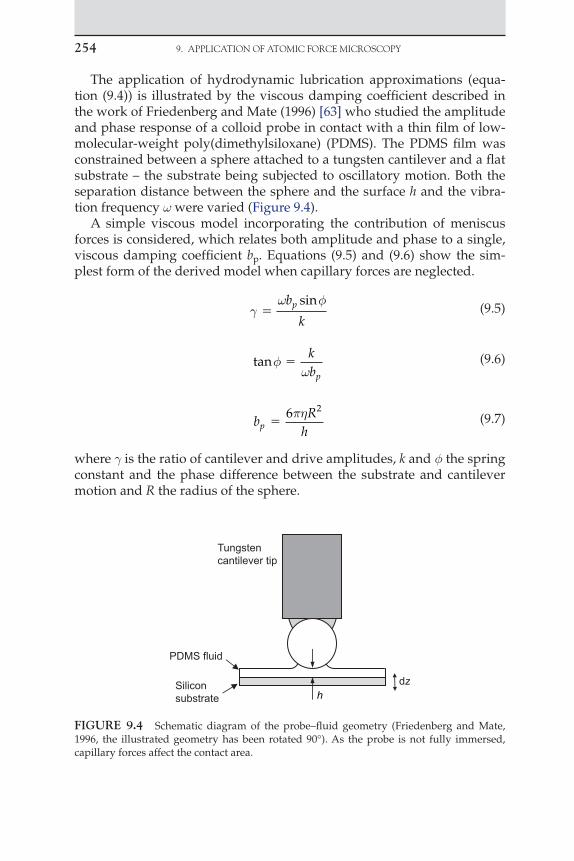
254 9. APPLICATION OF ATOMIC FORCE MICROSCOPy
The application of hydrodynamic lubrication approximations (equa-tion (9.4)) is illustrated by the viscous damping coefficient described in the work of Friedenberg and Mate (1996) [63] who studied the amplitude and phase response of a colloid probe in contact with a thin film of low-molecular-weight poly(dimethylsiloxane) (PDMS). The PDMS film was constrained between a sphere attached to a tungsten cantilever and a flat substrate – the substrate being subjected to oscillatory motion. Both the separation distance between the sphere and the surface h and the vibra-tion frequency were varied (Figure 9.4).
A simple viscous model incorporating the contribution of meniscus forces is considered, which relates both amplitude and phase to a single, viscous damping coefficient bp. Equations (9.5) and (9.6) show the sim-plest form of the derived model when capillary forces are neglected.
φ
b
kp sin
(9.5)
tanφ
kbp
(9.6)
b
Rhp
6 2π
(9.7)
where is the ratio of cantilever and drive amplitudes, k and φ the spring constant and the phase difference between the substrate and cantilever motion and R the radius of the sphere.
Siliconsubstrate
PDMS fluid
Tungstencantilever tip
hdz
FIguRE 9.4 Schematic diagram of the probe–fluid geometry (Friedenberg and Mate, 1996, the illustrated geometry has been rotated 90°). As the probe is not fully immersed, capillary forces affect the contact area.

The value of the viscous damping coefficient bp is then determined by fitting the measured values of both amplitude and phase as a function of separation distance h to equations (9.5) and (9.6). The apparent viscosity of the fluid may then be calculated from the damping coefficient and equation (9.7). Using this method reasonable agreement between the cal-culated viscosity and measured ‘bulk’ viscosity was found; however, the results also indicated that the surface roughness of the sphere may cause deviations from the expected zero-intercept relationship inferred from equation (9.7) (i.e. 1/bp vs. h). Choi and Kato (2003) [64] have extended this approach to investigate the shear properties of perfluoropolyether liquid bridges formed between two glass spheres by inducing lateral oscil-lations (as opposed to the normal perturbations depicted in Figure 9.4).
Suraya et al. (2008) [62] have reported the use of dynamic AFM to investigate the viscoelastic response of adsorbed hydroxypropyl guar (HPG) layers. The results identified dominant viscous properties at large surface separations and viscoelastic behaviour at closer separations where the polymer layers interact. The adsorbed polymer also exhibited viscoelastic frequency dependence and ‘shear thinning’ characteristics.
Similar studies were performed by Braithwaite and Luckham (1999) [65] who studied the viscoelastic response of adsorbed layers of gelatine under compression using dynamic modulation. The system consisted of a colloid probe interacting with a hard substrate where both surfaces were coated with a thin film of adsorbed gelatine. The model employed considers the characteristics of the viscoelastic materials as discussed by Radmacher et al. (1993) [66].
In such studies, as the actual values of stress and strain in the sample cannot be determined directly, they are instead speculatively related to the force F and displacement z of the cantilever through the use of an ‘apparatus coefficient’ b such that for a given frequency:
ε
Gb
Fz
*1
(9.8)
From which an alternative definition of the storage and loss moduli may be described [65, 66] wherein the equations are of the form:
′G
kb
( )(cos )
cos
φ
φ
2 2 1
(9.9)
and
′′G
kb
( )sin
cos
φ
φ
2 2 1
(9.10)
9.3 dyNAMIC MOdULATION STUdIES ON CONFINEd FLUIdS 255
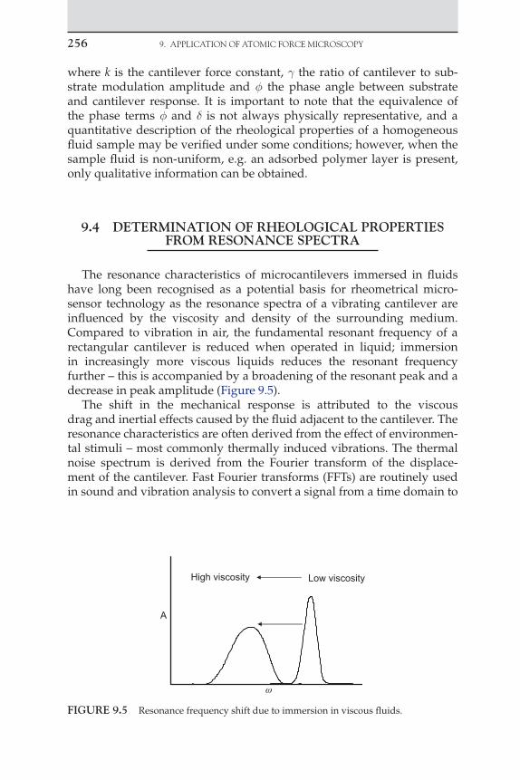
256 9. APPLICATION OF ATOMIC FORCE MICROSCOPy
where k is the cantilever force constant, the ratio of cantilever to sub-strate modulation amplitude and φ the phase angle between substrate and cantilever response. It is important to note that the equivalence of the phase terms φ and is not always physically representative, and a quantitative description of the rheological properties of a homogeneous fluid sample may be verified under some conditions; however, when the sample fluid is non-uniform, e.g. an adsorbed polymer layer is present, only qualitative information can be obtained.
9.4 DETERMInATIon oF RhEoLogICAL PRoPERTIES FRoM RESonAnCE SPECTRA
The resonance characteristics of microcantilevers immersed in fluids have long been recognised as a potential basis for rheometrical micro-sensor technology as the resonance spectra of a vibrating cantilever are influenced by the viscosity and density of the surrounding medium. Compared to vibration in air, the fundamental resonant frequency of a rectangular cantilever is reduced when operated in liquid; immersion in increasingly more viscous liquids reduces the resonant frequency further – this is accompanied by a broadening of the resonant peak and a decrease in peak amplitude (Figure 9.5).
The shift in the mechanical response is attributed to the viscous drag and inertial effects caused by the fluid adjacent to the cantilever. The resonance characteristics are often derived from the effect of environmen-tal stimuli – most commonly thermally induced vibrations. The thermal noise spectrum is derived from the Fourier transform of the displace-ment of the cantilever. Fast Fourier transforms (FFTs) are routinely used in sound and vibration analysis to convert a signal from a time domain to
Low viscosityHigh viscosity
ω
A
FIguRE 9.5 Resonance frequency shift due to immersion in viscous fluids.

a frequency domain such that the relative magnitude of each frequency component may be evaluated and the resonance spectrum constructed.
The motion of the cantilever may be modelled as a simple harmonic oscillator (SHO) with an increased effective mass due to the contribu-tion of the fluid in close proximity to the beam. Simple approximations describing the contribution of the fluid mass are described by Oden et al. (1996) [83], who model the virtual mass of the SHO as the combination of the cantilever mass and the mass of a spherical fluid volume envelop-ing the cantilever. More advanced models are considered by Sader (1998) [67], who present analytical expressions for the hydrodynamic functions, which determine the hydrodynamic loading due to the motion of the mass of fluid around a rectangular beam. The theory considers cantile-vers with rectangular and cylindrical cross-sections for which the length is far greater than the diameter or width, respectively.
For beams of a circular cross-section, the analytical expression for the hydrodynamic function has been established previously; however, rect-angular beams of finite thickness are far more complicated to describe. Sader (1998) derives a correction factor () which relates the circular cross-section solution to that of an infinitely thin rectangular cantilever based on the approximate relationship previously described by Tuck (1969) [69] such that the hydrodynamic function rect is given by:
rect circ( ) ( ) ( ) (9.11)
where the correction factor () is of the form
( ) ( ) ( ) r ii (9.12)
and
r i f( ), ( ) (Re) (9.13)
For small amplitude oscillations, the characteristic Reynolds number depends upon the cantilever width x such that:
Re
fluid x2
4 (9.14)
For an SHO the amplitude A() is given by
AA
Q
R
RR
( )
≅
( )
02
2 2 2 2 2
2
12
(9.15)
9.4 dETERMINATION OF RHEOLOgICAL PROPERTIES FROM RESONANCE SPECTRA 257

258 9. APPLICATION OF ATOMIC FORCE MICROSCOPy
where A0 is the zero-frequency amplitude response, and R are the radial and radial resonant frequencies, respectively [70],
π
Rvacuum
r Rx
14
21
2 ( )
(9.16)
and
Q x r R
i R
4
2
π
( )
( )
(9.17)
where (cxt) is the mass per unit length of the cantilever of density c, width x and thickness t. r and i are the real and imaginary parts of the aforementioned hydrodynamic function ().
For an unknown fluid, the fundamental resonance profile is used to determine R and Q from equation (9.15). The method is not restricted to the use of the fundamental resonance mode, and higher resonance peaks may be used although the accuracy of the result is reduced. Provided vacuum is known, the experimentally determined values of the resonance frequency and the quality factor may then be used to determine the vis-cosity and density by numerically solving equations (9.16) and (9.17).
The SHO model is useful for the determination of both viscosity and density provided Q 1. If the cantilever response is heavily damped, Q 1, then the SHO model is not valid. However, this may in some instances be circumvented by the selection of a cantilever with different mechanical properties.
Maali et al. (2005) [71] have evaluated a simplified approximation for the hydrodynamic function () and propose that
r a a( )
1 2
(9.18)
and
i a a( )
3 4
2
(9.19)
where a1, a2, a3 and a4 are constants and is the characteristic thickness of fluid surrounding the cantilever equivalent to an exponential damping length , where
2
fluid

The accuracy of the model proposed by Sader (1998) was evaluated using several fluids including air, water, acetone, carbontetrachloride and butanol, which presented wide viscosity and density ranges. Results were presented for both precision fabricated and standard cantilevers, and in both cases the theoretical and experimental results for the Q fac-tor and resonant frequency as determined from the thermal resonance spectra were in close agreement [72] as were the viscosity and density results [70], which were found to be in accordance with known bulk measurements.
The resonance methods described provide a basis for the in situ deter-mination of both viscosity and density of inelastic liquids. However, the use of resonance data to elucidate viscoelastic parameters is extremely complicated. In this respect, the use of a modified Langevin model which incorporates a complex drag coefficient in an attempt to overcome the limitations of the simplified SHO model has also been studied [73–75].
9.5 CAvITATIon AnD ADhESIvE FAILuRE oF ThIn FILMS
Due to the high deformation rates which typify many mesoscale phe-nomena, such as film splitting, filamentation and cavitation processes, significant viscoelastic effects may be anticipated. One such effect is a delay in the cavitation of viscoelastic liquids in micrometre-sized gaps, due to the development of normal stresses [76]. Others claimed that viscoelastic effects include a displacement of the point of cavitation from the centre of contact (where film thickness is a minimum) and enhanced film thicknesses [77]. Little is known about the influence of viscoelasticity in sub-micron liquid film cavitation, but the initial film thickness is a crucial factor: for sufficiently thin films, even ostensibly low rates of surface separation may provoke the high rates of fluid deformation nec-essary to generate enough tension (through viscous forces) to result in cavitation [78].
It is important to realise that in ultrathin films of water, cavitation may occur spontaneously, due to the antipathy between the liquid and hydro-phobic surfaces between which it is confined [79]. Spontaneous cavitation was first observed experimentally by Christenson and Claesson (1988) [79]. Theory predicts that vaporous cavities will only form in pure liquids as a result of large tensions, some 1300–1400 bar in the case of water [80], although a somewhat higher figure (ca. 1900 bar) results from an inter-pretation of the thermodynamic properties of stretched water known as the stability limit conjecture [81]. Experiments involving very small quantities of pure water have produced tensions close to this homoge-neous nucleation limit [82], but they are not commonly observed.
9.5 CAvITATION ANd AdHESIvE FAILURE OF THIN FILMS 259

260 9. APPLICATION OF ATOMIC FORCE MICROSCOPy
Berard et al. (1993) [83] showed that the free energy of a bridging cavity is lower than that of liquid water when the surfaces are separated as far as micrometres and claim that the fact that such cavities are not observed as the two surfaces approach contact from far apart indicates that the liquid between them is metastable, i.e. there is some barrier preventing cavita-tion. The theory for the long-ranged hydrophobic attraction relies upon this notion of induced cavitation – the force between two colloids in a near-critical or a near-spinodal fluid is attractive and long-ranged – and the connection between the spinodal attractions in the bulk and measured long-range attractions between hydrophobic surfaces is the observed cavitation [84].
Computer simulations by Berard et al. [83] on a Lennard–Jones liquid confined between hard walls showed cavitation at small separations, and that there was indeed a spinodal separation. Approaching this separation it was found that the attractions were much stronger than the van der Waals attraction and longer ranged. Qualitatively, a separation-induced spinodal can account for the measured hydrophobic attractions.
In the case of cavitation which results from the development of fluid mechanical stresses (as tension), Joseph [78] has pointed out that the con-cept of ‘negative pressure’ is not particularly useful; it is more pertinent to consider the state of stress experienced by a liquid. In doing so, it is con-venient to decompose the stress into a deviator and mean normal stress, the most positive value of principal stresses being the maximum tension. In order to facilitate a comparison of a liquid’s cavitation threshold stress with the principal stresses at each point within the liquid, it is necessary to know the flow field. In terms of studying cavitation inception within mesoscale liquid films, this requirement imposes stringent experimental demands as it requires a comparison of the cavitation threshold at each point in a liquid sample with the principal stresses there. For liquids in motion, cavitation criteria must be based not on the pressure, but on the stress, and a cavitation bubble will open in the direction of maximum ten-sion in principal coordinates. An important point which emerges is that a liquid can cavitate as a result of experiencing a shear deformation, the resulting cavity being pulled open by tension in the direction defined by principal stresses.
Of the few experimental techniques capable of working at (or below) the mesoscale, the various ‘force microscopes’, such as the SFA, have been the most successful, but instances of their use in studies of thin fluid films are comparatively rare. Notable exceptions are provided by the work of Israelachvili and co-workers [85] who observed the growth and disappear-ance of vapour cavities in liquid films between separating mica surfaces in SFA experiments. The growth of a cavity was claimed to represent a ‘new’ cavitation damage mechanism, insofar as surface damage occurred dur-ing cavity inception [86]. This is an interesting finding given that by far

the greatest effort in cavitation damage research has involved the study of bubble collapse and its consequences. Lord Rayleigh’s seminal analysis of the collapse of an isolated spherical void in an incompressible liquid [87] leads to the conclusion that, as the collapse nears completion, the pressure inside the liquid becomes indefinitely large. It is principally this ‘Rayleigh collapse’ mechanism (albeit extensively modified) which has led to the association of bubble collapse with cavitation damage [88].
Little is known about the dynamics of cavities formed in thin films but, due to their inevitably close proximity to the film’s bounding surfaces, sig-nificant departures from spherical symmetry may be anticipated [89]. The asymmetry of cavity collapse leads to potentially damaging phenomena, such as liquid jets [90], but the issue of cavitation damage due to cavity growth has received relatively little attention, despite the possibly damaging consequences to capillaries and small blood vessels due to the intraluminal expansion of cavitation bubbles in the areas of laser angioplasty [91], electrohydraulic lithotripsy [92] and shock wave lithotripsy [93].
9.6 MESoSCALE ExPERIMEnTAL STuDIES oF ThE TEnSILE BEhAvIouR oF ThIn FLuID FILMS
As discussed, many processes of emerging scientific and technological interest involve the rheological behaviour of complex fluids in the mesoscale domain (ca. 0.1–10 m), and in order to study the mesoscopic behaviour of fluids, particularly filament formation (i.e. extensional flow) and cavitation-induced failure and tack, it is necessary to satisfy some basic requirements. Notwithstanding the fact that the creation of a liquid bridge between a col-loid probe and a flat surface is a fairly straightforward process, manipula-tion of the desired quantity of fluid is not. Therefore in addition to recording the evolution of tensile forces, the deformation of the fluid should ideally be recorded. Although instruments such as the AFM suggest themselves for adaptation in terms of the former requirement, the latter task (i.e. recording the deformation of mesoscale filaments with sufficient temporal resolution) is non-trivial. But it is one which must be accomplished as a precursor to the development of a satisfactory mesoscale extensional flow technique.
Extensional flows of complex fluids may be studied using several mac-roscale techniques such as the filament stretching rheometer (FSR) or the capillary break-up extensional rheometer (CaBER), whose illustrations are shown in Figures 9.6 and 9.7. In these techniques the characteristic dimen-sions and the quantity of liquid are known, whereas the interpretation of results from AFM-based microrheometry is restricted by the necessary assumptions about the flow field.
As a colloid probe moves rapidly away from a surface, it is reasonable to assume that the fluid confined between the surface and the sphere may
9.6 MESOSCALE ExPERIMENTAL STUdIES 261

262 9. APPLICATION OF ATOMIC FORCE MICROSCOPy
be extended. If the initial minimum separation distance is sub-micron and the retraction event is sufficiently rapid, then the stresses generated within the liquid may approach or exceed the tensile strength of the liq-uid. However, in AFM studies the fluid is not directly observed, therefore fluid draining, viscoelastic filamentatious behaviour or cavitational fail-ure is not readily substantiated. It is, therefore, useful to examine those means by which the deforming liquid can be observed and documented. The separation distances considered in most AFM force studies are near to, or beyond, the limits of conventional optical microscopy. Although it is not possible to observe nanofilaments through an optical microscope,
FIguRE 9.6 Formation of macroscopic viscoelastic liquid filaments formed in a filament stretching rheometer. The fluid is constrained between the ends of two cylinders, which are pulled apart at a specified rate. The generated tensile force and the filament profile are used to calculate the extensional stress. The cylinder shown is 10 mm in diameter.
FIguRE 9.7 Images showing a typical CaBER experiment on a biopolymer solution. The surfaces are separated at a predetermined distance, thereafter the temporal evolution of the surface profile is used to determine rheological properties. Cylinder diameter is 2 mm.
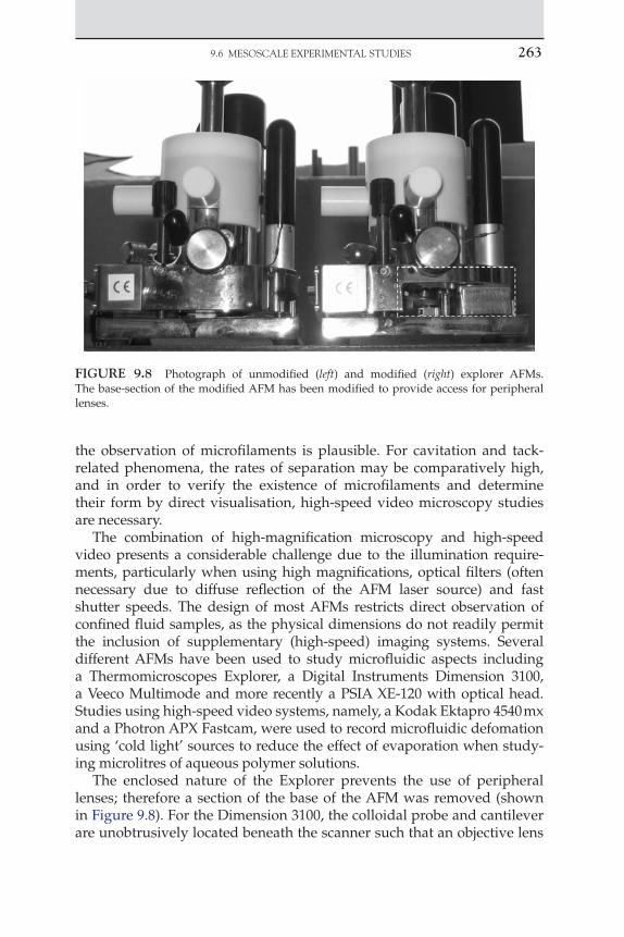
the observation of microfilaments is plausible. For cavitation and tack-related phenomena, the rates of separation may be comparatively high, and in order to verify the existence of microfilaments and determine their form by direct visualisation, high-speed video microscopy studies are necessary.
The combination of high-magnification microscopy and high-speed video presents a considerable challenge due to the illumination require-ments, particularly when using high magnifications, optical filters (often necessary due to diffuse reflection of the AFM laser source) and fast shutter speeds. The design of most AFMs restricts direct observation of confined fluid samples, as the physical dimensions do not readily permit the inclusion of supplementary (high-speed) imaging systems. Several different AFMs have been used to study microfluidic aspects including a Thermomicroscopes Explorer, a Digital Instruments Dimension 3100, a Veeco Multimode and more recently a PSIA XE-120 with optical head. Studies using high-speed video systems, namely, a Kodak Ektapro 4540 mx and a Photron APX Fastcam, were used to record microfluidic defomation using ‘cold light’ sources to reduce the effect of evaporation when study-ing microlitres of aqueous polymer solutions.
The enclosed nature of the Explorer prevents the use of peripheral lenses; therefore a section of the base of the AFM was removed (shown in Figure 9.8). For the Dimension 3100, the colloidal probe and cantilever are unobtrusively located beneath the scanner such that an objective lens
9.6 MESOSCALE ExPERIMENTAL STUdIES 263
FIguRE 9.8 Photograph of unmodified (left) and modified (right) explorer AFMs. The base-section of the modified AFM has been modified to provide access for peripheral lenses.

264 9. APPLICATION OF ATOMIC FORCE MICROSCOPy
may be positioned adjacent to the cantilever holder. For the multimode system, a light intensified high-speed camera (an APX I2 intensified head) was employed due to illumination restrictions. Photomicrographic studies using the XE-120 (optical head system) are readily achieved as the optical head system permits peripheral access.
The selection of a suitable microscope assembly is determined prin-cipally by the minimum attainable distance between lens and colloid probe; therefore ultralong working distance (ULWD) lenses were used (with supplementary lenses) as shown in Figure 9.9.
Separation of the surfaces is achieved either by raising the probe (con-ventional force–distance) or by lowering the sample substrate using a piezoceramic actuator. The Explorer is especially suited to the latter as it may be positioned above an independent piezoceramic stack.
Figure 9.10 shows filamentatious behaviour of a viscoelastic polymer (the V-shaped cantilever is 85 µm long). The fluid is stretched between
FIguRE 9.9 The high-speed optical microscopy system incorporating (1) APX Fastcam high-speed camera, (2) extension tube, (3) supplementary macrolens magnification and motorised focus, (4) light source and (5) ULWD microscope lens.
FIguRE 9.10 Formation of microscale viscoelastic liquid filament formed between a V-shaped cantilever and a reflective silica substrate.

a ‘bare’ cantilever and a reflective silica substrate, the reflected image is apparent in the lower half of the figure. When probeless cantilevers are brought into contact with liquid layers or drops, the cantilever is often enveloped by the fluid. In this respect the use of a colloid probe can help prevent wetting of the cantilever beam and the associated degradation of the laser signal.
Figure 9.11(a) shows a colloid probe attached to the tip of a V-shaped cantilever supported underneath the dimension scanner. In this example, no optical filters are used as careful alignment of both the optical micro-scope and the focal point of the laser reduces the transmission of diffuse laser light to the camera; although diffuse reflections are apparent (on the right hand side of the image), they are not excessive. If the observation angle is varied, such that the cantilever is viewed slightly from above, then either (i) optical filters are used or (ii) the field of view of the micro-scope is adjusted to omit all but the tip of the cantilever (under the same illumination conditions, omission of the optical filters permits higher photographic recording rates). This method is not employed using a light intesified system as the intensifier could be irreparably damaged. Figure 9.11(b) shows the interaction between a 15-m diameter colloid probe and a ‘large’ droplet of silicon oil, which is spread upon a reflective silica substrate. When first brought into contact, the silicon oil immediately enveloped the sphere and also adhered to the underside of the cantile-ver even though the cantilever was far above the surface of the drop; this effect was not readily apparent from above (as observed via the integrated AFM optics). The image shows the non-ideal liquid geometry during the
9.6 MESOSCALE ExPERIMENTAL STUdIES 265
(a) (b)
FIguRE 9.11 (a) A colloid probe attached to the end of a V-shaped cantilever as observed using the optical system shown in Figure 9.9. The cantilever is observed directly from the side, hence the V-shape is not apparent. (b) The partial envelopment of a 15-m diameter colloid probe by an excess of silicon oil ( 12 Pa s).
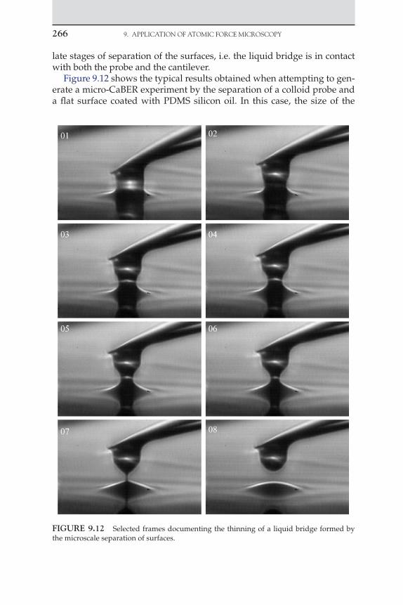
266 9. APPLICATION OF ATOMIC FORCE MICROSCOPy
late stages of separation of the surfaces, i.e. the liquid bridge is in contact with both the probe and the cantilever.
Figure 9.12 shows the typical results obtained when attempting to gen-erate a micro-CaBER experiment by the separation of a colloid probe and a flat surface coated with PDMS silicon oil. In this case, the size of the
FIguRE 9.12 Selected frames documenting the thinning of a liquid bridge formed by the microscale separation of surfaces.

sphere and the thickness of the fluid layer are such that only the under-side of the colloid is wetted. In frame 01, meniscus effects can be seen, when the surfaces are separated, a microscale liquid bridge is formed, which persists at large separations. The liquid bridge thins until the fila-ment fails between frames 07 and 08, leaving residual liquid on both the probe and the lower surface. The evolution of the filament profile closely resembles the macroscale CaBER results shown in Figure 9.7.
Figure 9.13 shows the behaviour of a thin liquid film during the ‘high-speed’ separation of the surfaces. In this instance, the high rates of separation and the high stress invoked in the fluid initially resist separation of the sur-faces. Ultimately, the confined liquid layer appears to yield spontaneously (frame 02), forming a residual filament (initially 10-m long and 1.3-m in diameter created at an apparent rate 5000 m s1. The liquid filament then thins and breaks, residual liquid can be observed in frame 04.
The adaptation of an AFM to act as a microrheometer has several potential benefits. In conventional rheometry, the generation of high rates of deformation is difficult, particularly so in extensional flow tech-niques where the defining strain rate is approximated by the relationship ε .U/h. The uniaxial rate of extension of cylindrical filaments between
separating surfaces is equal to the ratio of the separation velocity U and the instantaneous length of the filament h.
9.6 MESOSCALE ExPERIMENTAL STUdIES 267
FIguRE 9.13 The high-speed separation of surfaces bridged by a thin film of silicon oil ( 12 Pa s). Frame interval is 2 m s.

268 9. APPLICATION OF ATOMIC FORCE MICROSCOPy
Therefore when the initial surface separation distance h is large, i.e. the initial characteristic length of the fluid sample is 1 mm, the attainment of moderate extensional rates (100 s1) requires an initial separation velocity 100 mm s1, which is readily achieved using linear drive sys-tems. However, the filament length must increase exponentially as a func-tion of time in order to maintain a constant rate of extension, a situation which most drive systems are unable to accommodate. Consequently, many tensile studies involving liquids are restricted to low rates of exten-sion (10 s1) or small total strains. In this respect, the recreation of elon-gational flows at the mesoscale using piezoceramic technology presents one possible method by which high extensional strain rates and large total strains may be achieved. Furthermore, the difficulties encountered when attempting to measure rapidly changing, small tensile forces, which are generated within low viscosity, liquid filaments may also be addressed by utilising the precise force measuring capabilities of the AFM.
The determination of tensile forces in flows which contain a dominant elongational component is readily achieved using an AFM force sensor; however, the ability to precisely determine elongational stress at large strains is only possible when the shape and size of the liquid layer is clearly understood. In this respect, it is necessary to document the evolu-tion of a microfilament to ascertain the minimum diameter such that the maximum tensile stress may be calculated. This is particularly important as the transient evolution of the profile of Newtonian and non-Newtonian liquid bridges may vary significantly such that a representation of the tensile stress through terms such as F/R2 may not be valid at large separa-tions. This is because the critical dimension (i.e. the filament diameter) is not simply related to separation distance and is itself dependent upon the viscoelastic properties of the material.
The ability of many fluid mechanical systems to perform the desired function is critically dependent upon the tensile properties of the material, and the inability of the fluid to sustain large tensions is often beneficial, e.g. in coating and lubricating flows. Characterisation of the shear, exten-sional and cavitational behaviour is clearly important, and the ability of an AFM to recreate high-rate deformations which are comparable to those encountered in industrial processes is of particular interest. Moreover, the ability to experimentally recreate film splitting, fibrillation and cavitational cohesive failure in one dynamic process is desirable. However, observa-tion of rapid microscale phenomena is not straightforward, especially so when cavitational mechanisms are encountered, as the observation of the growth and collapse of vapourous cavities requires microsecond tempo-ral resolution. Future work will extend the capabilities of the AFM–optical microscopy system to further investigate the presence and influence of cav-itational effects prior to the apparent cohesive failure of lubricant layers. As such, it is necessary to evolve the design of the experiment and in the first
instance it is intended to conduct additional microscopic observations from beneath the liquid layer. In this way, the current restrictions imposed by the focal distance can be reduced (it is necessary to use ULWD dry lenses to document filament formation), and high numerical aperture oil immersion lenses may be employed to study microscale cavitational effects in the thin fluid layer prior to the mesoscale deformation process.
ACknowLEDgEMEnTS
The authors would like to acknowledge Prof. W. Richard Bowen and Prof. Nidal Hilal for their significant contribution to the research content presented in section 9.6. The authors are grateful for the financial support of the EPSRC, the work reported here was conducted under EPSRC grant no. GR/S10438/01.
LIST oF SyMBoLS
A Cantilever vibration amplitude man ConstantB Geometric apparatus coefficient mbp Viscous damping coefficient N s m1
F Force NG* Complex modulus PaG’′ Elastic modulus PaG“″ Viscous modulus PaH Separation distance between probe and surface mK Spring constant N m1
R Radius of sphere mT Cantilever thickness mU Relative separation velocity m s1
X Cantilever width mZ Displacement m Ratio of cantilever and drive amplitudecirc Hydrodynamic function for cylindrical cantileverrect Hydrodynamic function for rectangular
cantilever Rheological phase angle °
LIST OF SyMbOLS 269

270 9. APPLICATION OF ATOMIC FORCE MICROSCOPy
ε Shear strain Shear viscosity Pa s Exponential damping length m Mass per unit length of cantilever kg m1
c Cantilever density kg m3
fluid Fluid density kg m3
Shear stress N m2
φ Phase difference between substrate and cantilever ° FrequencyR Resonant frequencyvacuum Resonant frequency in vacuum Correction factor
References [1] G. Binnig, C.F. Quate, Ch. Berger, Atomic force microscope, Phys. Rev. Lett. 56 (9)
(1986) 930–933. [2] W.W. Scott, B. Bhushan, Use of phase imaging in atomic force microscopy for meas-
urement of viscoelastic contrast in polymer nanocomposites and molecularly thick lubricant films, Ultramicroscopy 97 (2003) 151–169.
[3] P.K. Hansma, J.P. Cleveland, M. Radmacher, D.A. Walters, P.E. Hillner, M. Bezanilla, M. Fritz, D. Vie, H.G. Hansma, C.B. Prater, J. Massie, L. Fukunaga, J. Gurley, V. Elings, Tapping mode atomic force microscopy in liquids, Appl. Phys. Lett. 64 (13) (1994) 1738–1740.
[4] D. Dowson, C.M. Taylor, Cavitation in bearings, Ann. Rev. Fluid Mech. 11 (1979) 35–66.
[5] Y.H. Zang, J.S. Aspler, M.Y. Boluk, J.H. De Grace, Direct measurement of tensile stress (“tack”) in thin ink films, J. Rheol. 35 (1991) 345–361.
[6] A. Unsworth, D. Dowson, V. Wright, Cracking joints. A bioengineering study of cavi-tation in the metacarpophalangeal joint, Ann. Rheum. Dis. 30 (1971) 348–358.
[7] H. Spikes, The borderline of elastohydrodynamic and boundary lubrication, Proc. Instn. Mech. Eng. 214 (2000) 23–37.
[8] M.T. Tyree, The cohesion-tension theory of sap ascent, J. Exp. Bot. 48 (1997) 1753–1765. [9] H. Lakrout, P. Sergot, C. Creton, Direct observations of cavitation and fibrillation in
a probe tack experiment on model acrylic pressure sensitive adhesive, J. Adhes. 69 (1999) 307–359.
[10] G.J.C. Braithwaite, G.H. McKinley, Microrheometry for studying the rheology and dynamics of polymers near interfaces, J. Appl. Rheol. 9 (1999) 27–33.
[11] A. Zosel, The effect of fibrillation on the tack of pressure sensitive adhesives, Int. J. Adhes. Adhes. 18 (1998) 265–271.
[12] H. Strasburger, Tacky adhesion, J. Colloid Sci. 13 (1958) 218–231. [13] W.H. Banks, C.C. Mill, Tacky adhesion – a preliminary study, J. Colloid Sci. 8 (1953)
137–147. [14] F.C. MacKintosh, C.F. Schmidt, Microrheology, Curr. Opin. Coll. Int. Sci. 4 (1999)
300–307.
[15] C. Clasen, G.H. McKinley, Gap-dependent microrheometry of complex liquids, J. Non-Newtonian Fluid Mech. 124 (2004) 1–10.
[16] A. Mukhopadhyay, S. Granick, Micro- and nanorheology, Curr. Opin. Coll. Int. Sci. 6 (2001) 423–429.
[17] P. Attard, Measurement and interpretation of elastic and viscoelastic properties with the atomic force microscope, J. Phys. Condens. Matter 19 (2007) 1–33.
[18] A. Maali, B. Bhushan, Nanorheology and boundary slip in confined liquids using atomic force microscopy, J. Phys. Condens. Matter 20 (2008) 1–11.
[19] J.N. Israelachvili, G.E. Adams, Measurement of the forces between two mica surfaces in aqueous solutions in the range 0–100 nm, J. Chem. Soc. Faraday Trans. 74 (1978) 975–980.
[20] E. Pelletier, J.P. Montfort, F. Lapique, Surface force apparatus and its application to nanorheological studies, J. Rheol. 38 (4) (1994) 1151–1168.
[21] C.D.F. Honig, W.A. Ducker, Squeeze film lubrication in silicone oil: experimental test of the no-slip boundary condition at solid–liquid interfaces, J. Phys. Chem. C 112 (2008) 17324–17330.
[22] M. Hennemeyer, S. Burghhardt, R.W. Stark, Cantilever micro-rheometer for the char-acterization of sugar solutions, Sensors 8 (2008) 10–22.
[23] N. Ahmed, D.F. Nino, V.T. Moy, Measurement of solution viscosity by atomic force microscopy, Rev. Sci. Instrum. 72 (2001) 2731–2734.
[24] N. Belmiloud, I. Dufour, A. Colin, L. Nicu, Rheological behavior probed by vibrating microcantilevers, App. Phys. Lett. 92 (2008) 41907.
[25] G.Y. Chen, T. Thundat, E.A. Wachter, R.J. Warmack, Adsorption-induced surface stress and its effects on resonance frequency of microcantilevers, J. Appl. Phys. 77 (8) (1995) 3618–3622.
[26] N.A. Burnham, R.J. Colton, Measuring the nanomechanical properties and surface forces of materials using an atomic force microscope, J. Vac. Sci. Technol. 7 (4) (1989) 2906–2913.
[27] B. Du, O.K.C. Tsui, Q. Zhang, T. He, Study of elastic modulus and yield strength of polymer thin films using atomic force microscopy, Langmuir 17 (2001) 3286–3291.
[28] J. Domke, M. Radmacher, Measuring the elastic properties of thin polymer films with the atomic force microscope, Langmuir 14 (1998) 3320–3325.
[29] W.A. Ducker, T.J. Senden, R.M. Pashley, Direct measurement of colloidal forces using an atomic force microscope, Nature 353 (1991) 239–241.
[30] O.I. Vinogradova, G.E. Yakubov, Dynamic effects on force measurements. 2. Lubrication and the atomic force microscope, Langmuir 19 (2003) 1227–1234.
[31] P.G. Hartley, F. Grieser, P. Mulvaney, G.W. Stevens, Surface forces and deformation at the oil–water interface probed using AFM force measurement, Langmuir 15 (1999) 7282–7289.
[32] R.E. Mahaffy, C.F. Shih, F.C. MacKintosh, J. Käs, Scanning probe-based frequency-dependent microrheology of polymer gels and biological cells, Phys. Rev. Lett. 85 (4) (2000) 880–883.
[33] J.L. Alonso, W.H. Goldmann, Feeling the forces: atomic force microscopy in cell biology, Life Sci. 72 (2003) 2553–2560.
[34] K.E. Bremmell, A. Evans, C.A. Prestidge, Deformation and nano-rheology of red blood cells: an AFM investigation, Coll. Surf. B Biointerfaces 50 (2006) 43–48.
[35] Y-Z. Hu, S. Granick, Microscopic study of thin film lubrication and its contributions to macroscopic tribology, Tribology Lett. 5 (1998) 81–88.
[36] G. Gillies, C.A. Prestidge, P. Attard, An AFM study of the deformation and nanorheol-ogy of cross-linked PDMS droplets, Langmuir 18 (2002) 1674–1679.
[37] G. Gillies, C.A. Prestidge, Interaction forces, deformation and nano-rheology of emul-sion droplets as determined by colloid probe AFM, Adv. Colloid Interface Sci. 108–109 (2004) 197–205.
REFERENCES 271

272 9. APPLICATION OF ATOMIC FORCE MICROSCOPy
[38] P.A. O’Connell, G.B. McKenna, Rheological measurements of the thermoviscoelastic response of ultrathin polymer films, Science 307 (2005) 1760–1763.
[39] J.H. Teichroeb, J.A. Forrest, Direct imaging of nanoparticle embedding to probe viscoelasticity of polymer surfaces, Phys. Rev. Lett. 91 (1) (2003) 16104.
[40] C.M. Mate, G.M. McClelland, R. Erlandsson, S. Chiang, Atomic-scale friction of a tungsten tip on a graphite surface, Phys. Rev. Lett. 59 (17) (1987) 1942–1945.
[41] G. Meyer, N.M. Amer, Simultaneous measurement of lateral and normal forces with an optical-beam-deflection atomic force microscope, Appl. Phys. Lett. 57 (20) (1990) 2089–2091.
[42] P.-E. Mazeran, J.-L. Loubet, Normal and lateral modulation with a scanning force microscope, an analysis: implication in quantitative elastic and friction imaging, Tribology Lett. 7 (1999) 199–212.
[43] M. Reinstädtler, U. Rabe, A. Goldade, B. Bhushan, W. Arnold, Investigating ultra-thin lubricant layers using resonant friction force microscopy, Tribology Int. 38 (2005) 533–541.
[44] D.F. Ogletree, R.W. Carpick, M. Salmeron, Calibration of frictional forces in atomic force microscopy, Rev. Sci. Instrum. 67 (9) (1996) 3298–3306.
[45] S. Moon, M.D. Foster, Near surface nanomechanical behavior of pressure-sensitive adhesives using lateral modulation scanning probe microscopy, Langmuir 18 (2002) 1865–1871.
[46] A. Paiva, N. Sheller, M.D. Foster, A.J. Crosby, K.R. Shull, Study of the surface adhesion of pressure-sensitive adhesives by atomic force microscopy and spherical indenter tests, Macromolecules 33 (2000) 1878–1881.
[47] J.P. Phillips, X. Deng, R.R. Stephen, E.L. Fortenberry, M.L. Todd, D.M. McClusky, S. Stevenson, R. Misra, S. Morgan, T.E. Long, Nano- and bulk-tack adhesive proper-ties of stimuli-responsive fullerene-polymer blends, containing polystyrene-block- polybutadiene-block-polystyrene and polystyrene-block-polyisoprene-block-polystyrene rubber-based adhesives, Polymer 48 (2007) 6773–6781.
[48] J.W.G. Tyrrell, P. Attard, Viscoelastic study using an atomic force microscope modified to operate as a nanorheometer, Langmuir 19 (2003) 5254–5260.
[49] C. Cottin-Bizonne, S. Jurine, J. Baudry, J. Crassous, F. Restagno, E. Charlaix, Nanorheology: an investigation of the boundary condition at hydrophobic and hydrophilic interfaces, Eur. Phys. J. E 9 (2002) 47–53.
[50] R. García, R. Pérez, Dynamic atomic force microscopy methods, Surf. Sci. Rep. 47 (2002) 197–301.
[51] N.A. Burnham, G. Gremaud, A.J. Kulik, P.-J. Gallo, F. Oulevey, Materials properties measurements: choosing the optimal scanning probe microscope configuration, J. Vac. Sci. Technol. B 14 (2) (1996) 1308–1312.
[52] P. Maivald, H.J. Butt, S.A.C. Gould, C.B. Prater, B. Drake, J.A. Gurley, V.B. Elings, P.K. Hansma, Using force modulation to image surface elasticities with the atomic force microscope, Nanotechnology 2 (1991) 103–106.
[53] A.A. Galuska, R.R. Poulter, K.O McElrath, Force modulation AFM of elastomer blends: morphology, fillers and cross-linking, Surface Interface Anal. 25 (1997) 418–429.
[54] B. Gotsmann, C. Seidel, B. Anczykowski, H. Fuchs, Conservative and dissipative tip–sample interaction forces probed with dynamic AFM, Phys. Rev. B 60 (15) (1999) 11051–11061.
[55] H. Watabe, K. Nakajima, Y. Sakai, T. Nishi, Dynamic force spectroscopy on a single polymer chain, Macromolecules 39 (2006) 5921–5925.
[56] S.M. Notley, S. Biggs, V.S.J. Craig, Application of a dynamic atomic force microscope for the measurement of lubrication forces and hydrodynamic thickness between sur-faces bearing adsorbed polyelectrolyte layers, Macromolecules 36 (2003) 2903–2906.

[57] R.M. Overney, D.P. Leta, C.F. Pictroski, M.H. Rafailovich, Y. Liu, J. Quinn, J. Sokolov, A. Eisenberg, G. Overney, Compliance measurements of confined polystyrene solu-tions by atomic force microscopy, Phys. Rev. Lett. 76 (8) (1996) 1272–1275.
[58] F. Oulevey, N.A. Burnham, G. Gremaud, A.J. Kulik, H.M. Pollock, A. Hammiche, M. Reading, M. Song, D.J. Hourston, Dynamic mechanical analysis at the submicron scale, Polymer 41 (2000) 3087–3092.
[59] J.B. Pethica, W.C. Oliver, Tip surface interactions in STM and AFM, Physica Scripta T19 (1987) 61–66.
[60] U. Rabe, S. Amelio, E. Kester, V. Scherer, S. Hirsekorn, W. Arnold, Quantitative deter-mination of contact stiffness using atomic force acoustic microscopy, Ultrasonics 38 (2000) 430–437.
[61] D.C. Hurley, K. Shen, N.M. Jennett, J.A. Turner, Atomic force acoustic microscopy meth-ods to determine thin-film elastic properties, J. Appl. Phys. 94 (4) (2003) 2347–2354.
[62] A.R. Suraya, P.F. Luckham, C.J. Lawrence, Shear thinning and frequency dependent behaviour of adsorbed polymer layers: Part I. Experimental aspects and a first order analysis, J. Non-Newtonian Fluid Mech. 148 (2008) 57–64.
[63] M.C. Friedenberg, C.M. Mate, Dynamic viscoelastic properties of liquid polymer films studied by atomic force microscopy, Langmuir 12 (1996) 6138–6142.
[64] J. Choi, T. Kato, Measurement on the shear properties of liquid nanomeniscus bridge, Tribology Int. 36 (2003) 475–481.
[65] G.J.C. Braithwaite, P.F. Luckham, The simultaneous determination of the forces and viscoelastic properties of adsorbed polymer layers, J. Coll. Int. Sci. 218 (1999) 97–111.
[66] M. Radmacher, R.W. Tillmann, H.E. Gaub, Imaging viscoelasticity by force modula-tion with the atomic force microscope, Biophys. J. 64 (1993) 735–742.
[67] P.I. Oden, G.Y. Chen, R.A. Steele, R.J. Warmack, T. Thundat, Viscous drag measure-ments utilizing microfabricated cantilevers, Appl. Phys. Lett. 68 (26) (1996) 3814–3816.
[68] J.E. Sader, Frequency response of cantilever beams immersed in viscous fluids with applications to the atomic force microscope, J. Appl. Phys. 84 (1998) 64–76.
[69] E.O. Tuck, J. Eng. Math. 3 (1969) 29. [70] S. Boskovic, J.W.M. Chon, P. Mulvaney, J.E. Sader, Rheological measurements using
microcantilevers, J. Rheol. 46 (4) (2002) 891–899. [71] A. Maali, C. Hurth, R. Boisgard, C. Jai, T. Cohen-Bouhacina, J.-P. Aime, Hydrodynamics
of oscillating atomic force microscopy cantilevers in viscous fluids, J. Appl. Phys. 97 (2005) 74907.
[72] J.W.M. Chon, P. Mulvaney, J.E. Sader, Experimental validation of theoretical models for the frequency response of atomic force microscope cantilever beams immersed in fluids, J. App. Phys. 87 (8) (2000) 3978–3988.
[73] M. Gelbert, M. Biesalski, J. Rühe, D. Johannsmann, Collapse of polyelectrolyte brushes probed by noise analysis of a scanning force microscope cantilever, Langmuir 16 (2000) 5774–5784.
[74] F. Benmouna, D. Johannsmann, Hydrodynamic interaction of AFM cantilevers with solid walls: an investigation based on AFM noise analysis, Eur. Phys. J. 9 (2002) 435–441.
[75] F. Benmouna, D. Johannsmann, Viscoelasticity of gelatin surfaces probed by AFM noise analysis, Langmuir 20 (2004) 188–193.
[76] A. Ouibrahim, D.H. Fruman, R. Gaudemer, Vapor cavitation in very confined spaces for Newtonian and non Newtonian fluids, Phys. Fluids 8 (1996) 1964–1971.
[77] T. Narumi, T. Hasegawa, Experimental study on the squeezing flow of viscoelastic fluids. 1. The effect of liquid properties on the flow between a spherical surface and a flat plate, Bull. JSME 29 (1986) 3731–3736.
[78] D.D. Joseph, Cavitation and the state of stress in a flowing liquid, J. Fluid Mech. 366 (1998) 367–378.
REFERENCES 273

274 9. APPLICATION OF ATOMIC FORCE MICROSCOPy
[79] K.H. Christenson, P.M. Claesson, Cavitation and the interaction between macroscopic hydrophobic surfaces, Science 239 (1988) 390–392.
[80] J.C. Fisher, The fracture of liquids, J. Appl. Phys. 19 (1948) 1062–1067. [81] R.J. Speedy, Stability-limit conjecture. An interpretation of the properties of water,
J. Phys. Chem. 86 (1982) 982–991. [82] Q. Zheng, D.J. Durben, G.H. Wolf, C.A. Angell, Liquids at large negative pressure:
water at the homogeneous nucleation limit, Science 254 (1991) 829–832. [83] D.R. Berard, P. Attard, G.N. Patey, Cavitation of a Lennard–Jones fluid between hard
walls, and the possible relevance to the attraction measured between hydrophobic surfaces, J. Chem. Phys. 98 (1993) 7236–7244.
[84] P. Attard, Bridging bubbles between hydrophobic surfaces, Langmuir 12 (1996) 1693–1695.
[85] Y.L. Chen, T. Kuhl, J. Israelachvili, Mechanism of cavitation damage in thin liquid films: collapse damage vs. inception damage, Wear 153 (1992) 31–51.
[86] T. Kuhl, M. Ruths, Y.L. Chen, J. Israelachvili, Direct visualisation of cavitation and damage in ultrathin liquid films, J. Heart Valve Dis. 3 (1994) 117–127.
[87] L. Rayleigh, On the pressure developed in a liquid during the collapse of a spherical cavity, Phil. Mag. 34 (1917) 94–98.
[88] M.S. Plessett, A. Prosperetti, Bubble dynamics and cavitation, Ann. Rev. Fluid Mech. 9 (1977) 145–185.
[89] J.R. Blake, D.C. Gibson, Growth and collapse of a vapour cavity near a free surface, J. Fluid Mech. I 11 (1981) 123–140.
[90] T.B. Benjamin, A.T. Ellis, The collapse of cavitation bubbles and the pressures thereby produced against solid boundaries, Phil. Trans. R. Soc. A 260 (1966) 221–240.
[91] T.G. von Leeuwen, J.H. Meertens, E. Velema, M.J. Post, C. Borst, Intraluminal vapor bubble induced by excimer laser pulse causes microsecond arterial dilation and invagination leading to extensive wall damage in the rabbit, Circulation 87 (1993) 1258–1263.
[92] R. Vorreuther, R. Corleis, T. Klotz, P. Bernards, U. Engelmann, Impact of shock wave pattern and cavitation bubble size on tissue damage during ureteroscopic electrohy-draulic lithotripsy, J. Urol. (Baltimore) 153 (1995) 849–853.
[93] P. Zhong, I. Cionta, S. Zhu, F.H. Cocks, G.M. Preminger, Effects of tissue constraint on shock wave-induced bubble expansion in vivo, J. Acoust. Soc. Am. 104 (1998) 3126–3129.

Atomic Force Microscopy in Process Engineering ©2009,ElsevierLtd275
FutureProspects
10C H A P T E R
The preceding chapters have shown that the use of AFM has already made substantial contributions to understanding and improving processes across a wide range of engineering. The literature on such applications is very extensive, so the aim of the present book has been to focus on some key examples in depth rather than to attempt a comprehensive overview, which would necessarily have been either unreasonably lengthy or else unsatisfyingly superficial. It is our hope that we have given an account of the principles, achievements and possibilities of AFM that is sufficiently informative for experts in other areas of process engineering to envisage how their own work may be enhanced using the techniques described. Owing to the broadness of the field, it is difficult to envisage where the most important developments are likely to take place in the future. How-ever, we have asked the authors of the preceding chapters to give a brief account as to how they would see the use of AFM in their own specialties developing, with the following results.
The importance of AFM lies in its capability to provide better under-standing of materials’ structure, surface characteristics and the interactive forces at the meso- and nanoscale level. This will greatly help understand large-scale engineering processes, especially as materials are increasingly being designed down to the submicrometre level. The developments of colloid, coated-colloid and cell probe techniques have already opened new windows of applications to a variety of engineering processes includ-ing those involving bubbles, such as flotation, and processes within the biotechnology sector. For example, characterisation of membrane surface morphology and forces of interaction with colloidal particles and cells has facilitated the development of synthetic membranes with greatly improved process-separation characteristics. As synthetic membranes play a key role in water treatment, including desalination, such use of AFM is likely to be an increasingly important application. Similarly, AFM studies of particle-bubble interactions can play a major role in optimising mineral separations, one of the largest-scale of all process operations. However,

276 10. FuTuREPRosPECTs
most AFM studies have so far been carried out under ambient conditions, whereas many industrial processes operate at reduced or elevated tem-peratures and pressures. The more recent development of hot–cold stages has made possible the application of AFM for both imaging and quantifi-cation of forces of interactions in the temperature range between 90°C and 250°C. Future development of pressure cells to enable the operation at both vacuum and pressures higher than atmospheric will further widen the range of process-relevant environments for further studies.
The application of process engineering knowledge to biotechnology and medicine is showing huge potential. The integration of cutting-edge techniques to develop tailored cellular micro-environments as model systems has proven essential for the systematic investigation of a num-ber of physiological processes in cell biology. From these studies, it has become apparent that restoring native functionalities using smart extra-cellular matrix (ECM), or tissue, depends on adequate consideration of interconnected processes that are regulated by biochemical, physical and mechanical factors in the ECM.
AFM, with its proven capability for nanoscale measurements of biomo-lecular interactions, and physical and mechanical properties of materials, is expected to continue to make invaluable contributions to cell biology and biotechnology fields. However, new developments are desirable to improve measurement reliability and to understand the factors that determine measurement reproducibility. In the same way as closed-loop scanners have greatly enhanced the metrological capabilities of AFM and hence the precision in measurement of large biological samples (such as living cells), there is still much scope for improvements associated with force measurements. This may be in the area of probe fabrication, providing cheap sources of cantilevers with high-tolerance spring constants or more likely in reliable, accurate, non-destructive and (hopefully) simple proto-cols for the calibration of existing probe types. Such improvements may in turn provide an impetus for the development and widespread use of mathematical modelling (such as the use of finite element techniques) to interpret force curves in the context of heterogeneous cellular structures – modern computing now makes such data fitting a tractable problem. Such approaches require close collaboration between biologists, engineers and physical scientists.
The integration of AFM and optical techniques for simultaneous inter-rogation of biochemical functionalities with physical/mechanical proper-ties of a cell offers huge benefits and is likely to attract increasing research efforts. High-speed optical imaging offers the possibility of monitoring processes that are currently too fast for AFM to interrogate. The present developments of high-speed AFM imaging are certainly encouraging. However, progress is required to minimise the tip-surface interactions that, at these speeds, greatly perturb the surface being imaged.

10. FuTuREPRosPECTs 277
In recent years, a number of complementary measurement probes have been integrated onto AFM tips, permitting the imaging of other properties of a sample simultaneously with its topography. These novel developments have included the incorporation of electrochemical, thermal, magnetic and electronic sensors. Researchers have also found that, in addition to being able to perform measurement functions, often these sensors allow the controlled alteration of the local environment around the tip. Preliminary work using certain types of sensors has shown that this feature could find great applicability in modulating micro- and nanoenvironments of living cells. Such functionalised probes could be incorporated into an existing AFM system, hence significantly enhancing its capability at modest cost. The availability of high-quality probes is also a factor limiting the uptake of some combined techniques, such as AFM and scanning near field opti-cal microscopy (SNOM). The combination of super-resolution optical and topographic imaging (AFM-SNOM) is certainly of great interest to biolo-gists because of the wealth of new information it could provide.
Polymers on surfaces play and will continue to play a major role in vari-ous engineering applications such as colloidal stabilisation, lab-on-a-chip devices, polymer composites and nanocomposites. Surprisingly, the signifi-cance of the polymer-solid interface region has been realised only relatively recently, and there are many gaps in our basic understanding. In nanocom-posites, the interface regions can be so extensive that they can occupy most of the overall volume of the material even at low or moderate nanoparticle loadings. Furthermore, the conformation and nature of entanglements of confined polymer chains in close proximity to a solid surface can deviate significantly from the bulk. As AFM is a real-space, high-resolution surface technique capable of probing quantitatively both the nanostructural and nanomechanical properties, it is likely to play an important role in the study of the interface region in polymer composites and nanocomposites.
The self-assembly and self-organisation of polymers on solid–liquid interfaces can be used as a generic technique for the inexpensive mass production of surface nanostructures and nanopatterns. Many issues remain to be elucidated by careful quantitative experimentation, and AFM is being proven to be an indispensable tool for the study of such systems in air or in liquids. Furthermore, the recent development of high-speed AFM with image-acquisition times in the order of a few milliseconds is an important development that could allow the monitoring of the mobility of polymer chains on a solid surface and consequently the kinetic paths of the nanostructures/nanopatterns formation. AFM offers the possibility for systematic studies of such systems that can elucidate the underlying physical mechanisms of the processes occurring on solid surfaces. These studies can lead in the construction of phase/state diagrams, which may be used for the design of well-controlled and specified surface nanostruc-tures for applications spanning from nanoelectronic devices to vectors for

278 10. FuTuREPRosPECTs
targeted drug/gene delivery. Further, AFM is becoming an indispensable characterisation tool of miniaturised device components, which increas-ingly involve the use of (bio)polymers, ultrathin films and nanostructures on surfaces.
To date, the successful use of AFM-based techniques to determine the viscoelastic properties of materials is exemplified by the successful use of indentation or compression experiments, for which established theoreti-cal models adequately describe the rheological properties. Of particular note are the developments in biomechanical studies, wherein the deter-mination of the viscoelastic response of cells and biological tissues using a combination of an AFM and a confocal laser scanning microscope (CLSM) is an interesting development, especially so with the use of modern fast-scanning CLSMs.
For fluids, although experimental studies have shown that an AFM is certainly capable of emulating the rheological capabilities of the surface forces apparatus (SFA), the use of an AFM to quantitatively describe the rheology of thin fluid films remains the subject of considerable research interest. Although, the viability of AFM as a micro-rheometrical tool has been established, the development of mathematical models capable of interpreting the response of microcantilevers in viscoelastic fluids is still evolving, and further development is vital to the successful applica-tion of this technique. Nevertheless, the integration of AFM cantilevers in microfluidic and other fluid sensor devices is a realistic option, enabled most significantly by advances in the description of viscous effects upon resonance characteristics. From a rheometrical perspective, this is partic-ularly encouraging as few other technologies can address the associated issues of scale. The development of this area will in part rely upon the fabrication of appropriate cantilever geometries, such that the resonance characteristics and sensitivity of the device are optimized for the fluid of interest. In this respect, the fabrication of multilevers on common sub-strates may extend the measuring capabilities and represents a potential enabling technology for the study of more complex, multicomponent flu-idic systems.
The adaptation of dynamic AFM methods for the routine rheologi-cal characterisation of thin fluid films is more problematical. However, qualitative results suggest that the technique has potential merits. The dynamic response of a vibrating probe is clearly able to detect the onset of viscoelastic behaviour, but quantitative rheological information as yet remains elusive. Surprisingly, many dynamic studies favour oscillation in the direction normal to the surface, and as such it may be anticipated that significant compressional wave components can influence oscilla-tion of the probe. For the analogous study of macroscale oscillatory shear and microscale rheometrical parameters, further studies on oscillatory microscale shear deformations would be beneficial.

10. FuTuREPRosPECTs 279
In either case, as the system response is not simply related to the stress and the strain in the fluid, there is at present no satisfactory way to quan-titatively determine the complex moduli. However, the promising results of studies to date suggest that an AFM operating in dynamic mode is suited to adaptation as a mechanical interferometer, i.e. a device that can be used to determine the ‘time of flight’ of small amplitude shear waves across a fluid-filled gap. This is analogous to the so-called virtual gap rheometer (VGR), wherein the phase delays determined at two different locations in the fluid can be used to determine the phase velocity of the shear wave. By studying several frequencies, the frequency-dependent behaviour of viscoelastic systems may be exploited to determine the gel point of curing polymers.
Most importantly, the future prospects of all applications of AFM in process engineering will be greatly enhanced by increased collaboration between engineers, physical scientists, biological scientists, mathematicians and instrument manufacturers. Among the most crucial of the multidisci-plinary themes that need to be addressed are the development of probes of highly specified and reproducible physical properties; the development of high-speed image acquisition so that dynamic processes may be followed; the combination of AFM with other techniques in a single instrument, especially techniques that allow chemical characterisation of surfaces and the integration of AFM data acquisition and advanced mathematical modelling software for data interpretation.

Index
AActin stress fiber, 197Adhesion, 67–70, 198, 202, 226, 234, 246
drug particles, 174–76, 178–79, 182, 184forces, 67–70, 81, 91–93, 97, 141–43,
151–63, 164–66particles to bubbles, 83–85, 90, 91particles to membranes, 112, 113, 122
Adhesives, 248–49AFM-optical microscope, 211Aggregation, 229, 236Apparatus coefficient, 255Arg-Gly-Asp (RGD), 197, 203–04Atomic force acoustic microscopy, 252
BBiaxial extension, 248Biocompatibility, 226Biofilms, 135Block copolymer, 228, 236–237Boundary conditions, 49
charge regulation, 49constant surface charge, 49constant surface potential, 49constant zeta potential, 49
Bovine Serum Albumin (BSA), 49
CCapillary forces, 10, 15, 18, 90, 94, 230Cauchy Plot, 41Cavitation, 246–47, 259–61Cell membrane, 197Collagen fibres, 205Cell model, 52Cell probe, 113Charging of surface, 44Chemisorption, 227Chloride ion binding, 51Coating flows, 247Colloid probe, 22–23, 32, 55, 69, 111, 112,
210, 248, 253–55, 265–67coated, 113membrane measurements, 151–63, 164–66particle bubble measurements, 82, 91–93,
96, 99
Colloidal gas aphrons, 95–97Colloidal lithography, 203, 207Cytoplasm, 197Cytoskeleton, 197, 212, 217Complex modulus, 252–53Confined fluids, 252–56, 259–67Contact angles, 88–91Contact mode, 9Convolution, 230–31Corrosion metal, 132Counterions, 47Critical flux, 123
DDamping coefficient, 254–55Density, 247, 256–59Derjaguin approximation, 33Derjaguin, Muller Toporov model,
67, 178Dewetting, 229, 236DLVO theory, 53–54, 154
forces, 54–58, 91, 93DMT model, see Derjaguin, Muller Toporov
modelDry powder inhalator, 174–76Dynamic AFM, 2, 10–11, 249–56
EEffective stiffness, 43Elastic modulus, 180–81
see also Young’s modulusElasticity, 214Electrical double layer interactions, 47–53
analytical solutions, 47numerical solutions, 48
Electromechanical oscillator, 252Electron beam lithography (EBL), 203, 208Extracellular matrix (ECM), 195, 205
proteins, 196, 197, 207Electropolishing, 130Electrostatic interactions, 111, 121, 227Entropic elasticity, 234Exponential damping length, 258Extensional flow, 261Extensional rheometer, 261
281
282 InDEx
FFilamentation, 259, 261–62, 264–67Film splitting, 247, 267Filopodia, 198, 207, 212Focal adhesion, 197–8Focal complex, 198Force between two spheres, 33Force distance curve, 111, 112, 117Force map, 250Force modulation, 12, 249Force oscillations, 61Force volume imaging, 11Formulation, 174–75, 178, 182, 185–87,
188–90Fourier transform, 256Friction force microscopy, 21, 248Frictional force mode, 12Frictional forces, 12, 63, 178–79, 248
see also Lateral forceFroth flotation, 82Functionalised surface, 199
GGouy-Chapman theory, 45–46Grafting density, 228, 231–233
HHamaker constant, 38–42
calculation of, 40pairwise addition, 38
Hardness, 180Hertz model, 12, 180–82, 214–7, 248High-speed video microscopy, 263Humic acid, 166Humic substances, 140Humidity, 175–77, 183, 186Hydration forces, 59–60Hydrodynamic drag, 66Hydrodynamic forces, 63, 84–85, 98–100Hydrodynamic function, 17, 257–58Hydrodynamic lubrication, 253–54Hydrophobic surfaces, 64
IImaging in liquid, 116, 123Indentation, 179–82, 215, 247, 251Inner Helmholtz plane (IHP), 46Integrins, 197Intermittent contact mode, see Tapping
modeIsopotential lines, 119
JJKR model, see Johnson, Kendall, Roberts
modelJohnson, Kendall, Roberts model, 12, 67,
84, 178
LLamellipodia, 198Living cells, 212–4Lateral force, 12–22, 248–49Lateral resolution, 226Lennard-Jones potential, 36–37Lifshitz theory, 38, 40Light intensifier, 264–65Line tension, 89Liquid bridge, 255, 261, 265–68Liquid structure, 58–59Loading force, 234–35
bubble, 97membrane, 151–60
Loss modulus, 253
MMacromolecules, 225, 229Membrane characterisation, 141Membranes, 57, 107–26
development, 124–26fouling, 57, 68, 140–44
Mesoscale, 246, 261Metal surfaces, 126Metastability, 260Microcontact printing, 201Micropatterning, 199Microsphere indentation, 210Microfilament, 264–67Microfiltration, 108Microfoams, 95–97Micromanipulator, 34Microrheometry, 247, 261–68Microsensor, 247Modification of filtration membranes,
139–68Molecular weight cut-off, 113Monolayers, 226–30, 233–34, 236–39Multiparticle interaction, 52–53
nNanofiltration, 108Nanoimprint lithography (NIL), 203Nanopatterning, 203, 226–28, 233Nanotopography, 205–6

InDEx 283
Natural organic matter, 140Negative pressure, 247Non-contact mode, 10–11Non-DLVO forces, 58
OOptical microscope, 262, 264Outer Helmholtz plane (OHP), 46
PParticle-bubble interactions, 81–106Pharmaceuticals, 173–90Phase angle, 250, 254–56Phase imaging, 10, 185–86Photolithography, 199Physisorption, 199Polymer demixing, 206Physisorption, 227, 230, 235Pinned micelles, 232Poisson-Boltzmann Equation, 45Polar liquids, 55Polymer brush, 228–36Polymer chains, 226–34, 237–41Polymer coatings, 225–26Pore size diameter, 115 distribution, 109,
110, 116, 118, 119Pore size distribution, 140, 147–50, 168Powders, 174–75Primary alcohols, 61
QQ factor, see Quality factorQuality factor, 17
RResonance spectra, 256–59Resonant frequency, 17, 21, 258Retardation, 40Reverse osmosis, 108Reynolds number, 257Rheology, 246, 252–56, 262Roughness, 42, 44, 55, 69–70, 115, 120, 128,
129, 134
SScanning probe lithography, 203Scanning thermal microscope, 186–90Self assembled monolayers (SAM), 199Self-assembly nanofabrication, 203SEM, 210
Shear strain, 252, 255Shear stress, 252, 255Simple harmonic oscillator, 257Soft lithography, 201Solvation forces, 58–62Spring constant, 176–77Spring constant calibration, 16–22Spring constants, 87Star polymers, 237–240Steel, 132Steric interactions, 62Storage modulus, 253Stress fiber, 208Surface electrical properties, 117
TTack, 247, 249Tapping mode, 10, 236–37, 240, 250TEM, 210Tension, 246, 259–60Theta solvents, 62Thin liquid films, 254, 260Three-phase contact, 83, 88–90, 94–95, 97Threshold force, 94–95, 97Torsional spring constant, 21–22
UUltrafiltration, 108Uniaxial extension, 267
Vvan der Waals forces, 35–44, 83–84,
91, 227Debye forces, 35–37Keesom forces, 35–37London dispersion forces, 35–37Measurement by AFM, 42
Viscoelasticity, 249, 252–53, 255, 259Viscosity, 247, 255–59
WWork of adhesion, 43, 84
YYoung equation, 88–89Young’s modulus (E), 180–82, 215, 247
see also Elastic modulus
ZZeroth-order Stern model, 51


