License Quotas and the Inefficient Regulation of Sin Goods: Evidence from the Washington Recreational Marijuana Market * Danna Thomas † January 15, 2018 Abstract This paper studies the welfare impacts of license quotas in markets for “sin goods.” License quotas not only affect market structure and reduce total sales, their implementation also creates allocative costs. Retail licenses are often restricted by geography, meaning licenses are not neces- sarily allotted to areas where they are most valuable. Furthermore, licenses may be distributed to firms randomly; hence, the most profitable potential entrants are not necessarily license re- cipients. A difficulty in studying license quotas is finding credible counterfactuals of unrestricted entry. Therefore, I first develop a three stage model that endogenizes firm entry decisions and incorporates spatial demand. I then estimate the model using a new firm-level data set from the Washington recreational marijuana market and use data on the participants in a marijuana retail license lottery to simulate counterfactual entry patterns. I find that allowing firms to enter freely at Washington’s current marijuana tax rate increases total surplus by 21.5% relative to a baseline simulation of Washington’s license quota regime. Geographic misallocation and random allocation of licenses account for 6.6% and 65.9% of this difference, respectively. Moreover, I study tax poli- cies that directly control for the marginal damages of marijuana consumption. Free entry with tax rates that keep the quantity of marijuana or THC consumed equal to baseline consumption increases welfare by 6.9% and 11.7%, respectively. While free entry with a non-uniform sales tax consistent with Washington’s geographic license restrictions increases efficiency by over 7%. * I am grateful to my advisors Katherine Ho, Francois Gerard, and Tobias Salz for their guidance. This paper benefited from conversations with Michael Riordan, Chris Conlon, Wojciech Kopczuk, and Zach Brown. Lin Tian, Jing Zhou, and Nandita Krishnaswamy also provided helpful comments. I also thank Brian Yauger, Jerry Derevyanny, and Logan Bowers for all their helpful insight into the inner workings of the Washington recreational marijuana market. All mistakes are my own. † Columbia University, [email protected]
Transcript
License Quotas and the Inefficient Regulation of Sin Goods:Evidence from the Washington Recreational Marijuana Market∗
Danna Thomas†
January 15, 2018
Abstract
This paper studies the welfare impacts of license quotas in markets for “sin goods.” Licensequotas not only affect market structure and reduce total sales, their implementation also createsallocative costs. Retail licenses are often restricted by geography, meaning licenses are not neces-sarily allotted to areas where they are most valuable. Furthermore, licenses may be distributedto firms randomly; hence, the most profitable potential entrants are not necessarily license re-cipients. A difficulty in studying license quotas is finding credible counterfactuals of unrestrictedentry. Therefore, I first develop a three stage model that endogenizes firm entry decisions andincorporates spatial demand. I then estimate the model using a new firm-level data set from theWashington recreational marijuana market and use data on the participants in a marijuana retaillicense lottery to simulate counterfactual entry patterns. I find that allowing firms to enter freelyat Washington’s current marijuana tax rate increases total surplus by 21.5% relative to a baselinesimulation of Washington’s license quota regime. Geographic misallocation and random allocationof licenses account for 6.6% and 65.9% of this difference, respectively. Moreover, I study tax poli-cies that directly control for the marginal damages of marijuana consumption. Free entry withtax rates that keep the quantity of marijuana or THC consumed equal to baseline consumptionincreases welfare by 6.9% and 11.7%, respectively. While free entry with a non-uniform sales taxconsistent with Washington’s geographic license restrictions increases efficiency by over 7%.
∗I am grateful to my advisors Katherine Ho, Francois Gerard, and Tobias Salz for their guidance. This paperbenefited from conversations with Michael Riordan, Chris Conlon, Wojciech Kopczuk, and Zach Brown. Lin Tian, JingZhou, and Nandita Krishnaswamy also provided helpful comments. I also thank Brian Yauger, Jerry Derevyanny, andLogan Bowers for all their helpful insight into the inner workings of the Washington recreational marijuana market. Allmistakes are my own.†Columbia University, [email protected]
1 Introduction
To mitigate negative externalities from the consumption of “sin goods” (e.g. tobacco products,
alcohol, marijuana, etc.), states commonly restrict entry into retail markets for the offending goods
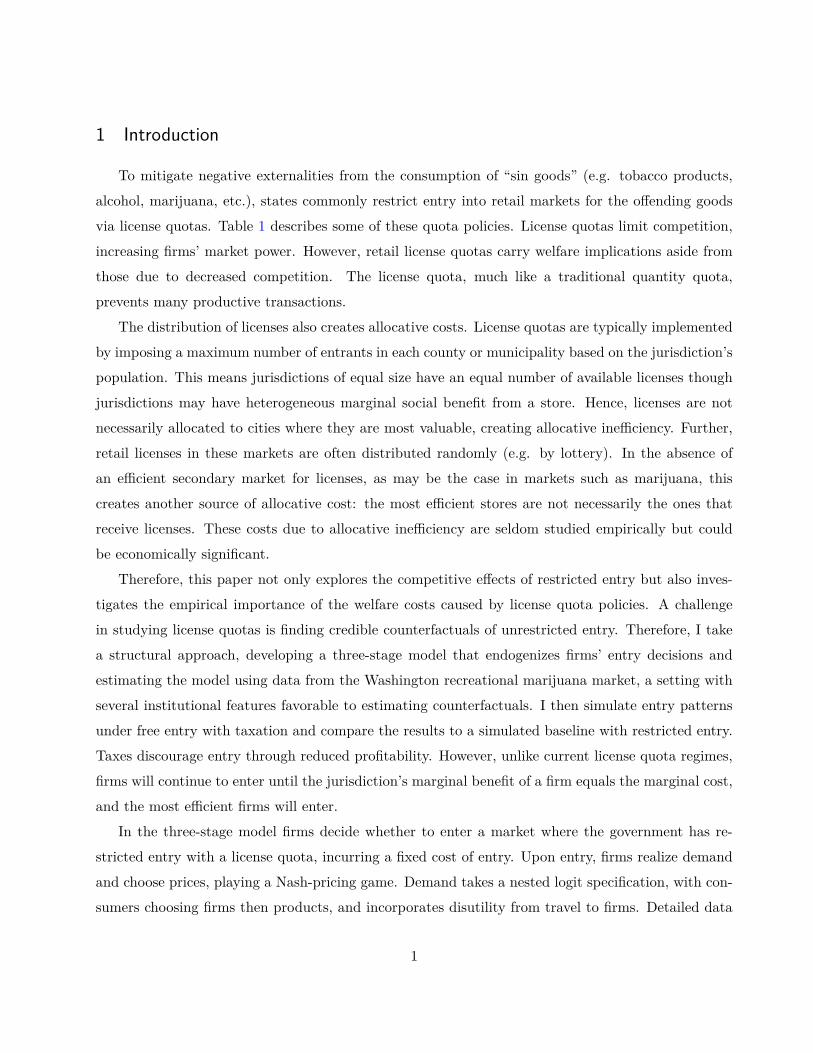
via license quotas. Table 1 describes some of these quota policies. License quotas limit competition,
increasing firms’ market power. However, retail license quotas carry welfare implications aside from
those due to decreased competition. The license quota, much like a traditional quantity quota,
prevents many productive transactions.
The distribution of licenses also creates allocative costs. License quotas are typically implemented
by imposing a maximum number of entrants in each county or municipality based on the jurisdiction’s
population. This means jurisdictions of equal size have an equal number of available licenses though
jurisdictions may have heterogeneous marginal social benefit from a store. Hence, licenses are not
necessarily allocated to cities where they are most valuable, creating allocative inefficiency. Further,
retail licenses in these markets are often distributed randomly (e.g. by lottery). In the absence of
an efficient secondary market for licenses, as may be the case in markets such as marijuana, this
creates another source of allocative cost: the most efficient stores are not necessarily the ones that
receive licenses. These costs due to allocative inefficiency are seldom studied empirically but could
be economically significant.
Therefore, this paper not only explores the competitive effects of restricted entry but also inves-
tigates the empirical importance of the welfare costs caused by license quota policies. A challenge
in studying license quotas is finding credible counterfactuals of unrestricted entry. Therefore, I take
a structural approach, developing a three-stage model that endogenizes firms’ entry decisions and
estimating the model using data from the Washington recreational marijuana market, a setting with
several institutional features favorable to estimating counterfactuals. I then simulate entry patterns
under free entry with taxation and compare the results to a simulated baseline with restricted entry.
Taxes discourage entry through reduced profitability. However, unlike current license quota regimes,
firms will continue to enter until the jurisdiction’s marginal benefit of a firm equals the marginal cost,
and the most efficient firms will enter.
In the three-stage model firms decide whether to enter a market where the government has re-
stricted entry with a license quota, incurring a fixed cost of entry. Upon entry, firms realize demand
and choose prices, playing a Nash-pricing game. Demand takes a nested logit specification, with con-
sumers choosing firms then products, and incorporates disutility from travel to firms. Detailed data
1
Table 1: Examples of License Quotas in Retail Markets
State/Locality Retailer Number of LicenseLicenses Distribution
Washington marijuana (2015) 334 state-wide lottery
Pennslyvania medical 27 state-wide points-basedmarijuana application process
San Francisco, CA tobacco 49 per supervisory district first-come, first-served
California liquor 1 per 2,500 people in county lottery
Massachusetts liquor 1 per 5,000 people in city/town first-come, first-served
Florida liquor 1 per 7,500 people in county lottery
Arizona liquor 1 per 10,000 people in county lottery
from the Washington recreational marijuana market on prices, quantities, and product characteristics
merged with demographic data allows me to estimate the demand system. The data also includes
wholesale costs which I use along with the Nash pricing equation to estimate a non-parametric dis-
tribution of costs. I then combine costs and demand to compute variable profits.
Estimating fixed costs involves using the logic of revealed preferences to infer the profitability
of firms. If n firms enter, then n firms are profitable, and firm n + 1 is not (Bresnahan and Reiss,
1991a). However, if there is a binding license quota, the profitability of firm n+ 1 cannot be inferred
(Schaumans and Verboven, 2008; Ferrari and Verboven, 2010). The Washington marijuana market,
though, has jurisdictions where retail license quotas do not bind, allowing me to draw the necessary
assumptions about profits to estimate fixed costs. Nonetheless, as is common in games of entry, a
multiplicity of equilibria exist, complicating the point identification of fixed costs. I, therefore, find
bounds on fixed costs using the moment inequalities methodology outlined in Pakes et al. (2015) and
Pakes (2010).
With the model and estimates in hand, I simulate counterfactual entry in those jurisdictions with
binding license quotas. A particularly difficult aspect of simulating entry in a model that incorporates
spatial demand is where to locate the simulated market entrants as it involves determining where firms
would have located if entry was not restricted. However, the Washington recreational marijuana
market provides me with plausible locations. After marijuana legalization, Washington regulators
opened an application window for retail licenses. Potential entrants needed to provide prospective
2
addresses on these license applications. For those jurisdictions with more applicants than available
licenses, the state distributed licenses via a lottery. I use addresses from applications not chosen in
the lottery to serve as counterfactual locations.
The first counterfactual exercise eliminates the license quota and simulates free entry, allowing
all profitable firms to enter. At Washington’s current marijuana tax rate of t = 0.37, I find that
the number of entrants increases by 60%—ninety-five additional firms; hence, license quotas severely
constrain firm entry in this market. Unrestricted entry also boosts total surplus by $23 million relative
to the baseline—an increase of 21.5%. This difference in surplus is because (1) less marijuana is sold
due to the license quota, and (2) licenses are not allocated efficiently under the quota regime.
To study the importance of allocative inefficiency, I decompose the difference in surplus between
the free entry simulation and the baseline. First, I simulate the outcome of a statewide license auction
without geographic license restrictions. By holding the number of licenses fixed to the baseline number
of total entrants, but not restricting the licenses by jurisdiction, or randomly distributing licenses,
this counterfactual measures the effect of the quota without allocative costs. Next, I generate the
outcome of a within-jurisdiction auction, keeping the number of licenses within each jurisdiction
equal to the jurisdiction’s baseline number of entrants. This captures the change in surplus due to
the misallocation of licenses over geography without capturing the cost of the license lottery.
The reduction in quantity sold due to the quota is responsible for 27.5% of the difference in surplus
between free entry and the baseline, and geographic license restrictions explains around 6.6%. The
allocation of retail licenses via lottery is the largest source of inefficiency, accounting for about 65.9%
of the loss in total surplus. Hence, allocative costs comprise over 70% of the efficiency loss due to
Washington’s license quota policy.
As governments may use license quotas as tools to mitigate externalities, I also study policies
that directly control for the marginal damages of marijuana consumption. To do this, I simulate free
entry while increasing the sales tax rate which deters entry and reduces consumption without creating
allocative costs. With free entry and a sales tax of t = 0.765, the amount of marijuana consumed is
the same as the quantity consumed in the baseline. Because there is no allocative inefficiency, total
surplus is 6.9% higher than in Washington’s license quota regime. The amount of THC consumed
remains equal to baseline consumption at t = 0.66 with total surplus increasing by almost 12%.
Because geographic license restrictions could be a way to account for hetergenous marginal dam-
ages across the state—meaning there is no misallocation of licenses across geography, I also simulate
3
free entry with a marijuana sales tax that varies across jurisdictions and is consistent with each juris-
diction’s license quota. This non-uniform sales tax produces a total surplus is 6.3% higher than the
baseline, highlighting the efficiency loss from allocating licenses randomly further.
This paper contributes to the literature on allocative costs. The theoretical literature is extensive
and discusses allocative costs in a variety of contexts (Deacon and Sonstelie, 1989; Bulow and Klem-
perer, 2012; Viscusi, Harrington, and Vernon, Viscusi et al.). However, the empirical importance
of allocative inefficiency is understudied, and to my knowledge no paper in the empirical literature
discusses retail license allocation. Notably, Glaeser and Luttmer (2003) studies misallocation due to
rent control policies. Davis and Kilian (2011) and Luttmer (2007) explore price ceilings in the U.S.
natural gas market and the labor market, respectively, and Frech and Lee (1987) analyze the welfare
cost of queuing during U.S. gasoline shortages in the 1970s. Further, these papers do not discuss
imperfect competition nor do they study allocative costs due to quantity regulation in markets with
negative externalities.
The size of allocative costs is particularly important in markets with negative externalities where
policy makers must choose between instruments such as taxation or quotas. Hence, this paper is also
related to the theoretical literature comparing corrective taxation to quantity regulation in mitigating
externalities (Weitzman, 1974; Kaplow and Shavell, 2002; Glaeser and Shleifer, 2001; Baumol and
Oates, 1971). An extensive discussion of this literature in the context of pollution abatement is
offered in Bovenberg and Goulder (2002).
My findings are also related to the industrial organization literature on firm entry and competition
(Bresnahan and Reiss, 1991b; Berry, 1992; Berry and Waldfogel, 1999; Seim, 2006; Mazzeo, 2002).
Frechette et al. (2016) study entry restrictions in the New York City taxi market albeit in a dynamic
model with a focus on search frictions. Most closely related to this paper is Schaumans and Verboven
(2008) which uses a model and empirical approach similar to Mazzeo (2002) to study license quotas in
the pharmacy market in Belgium though the study does not focus on the misallocation of licenses but
rather on the competitive effects of restricted entry. My empirical approach is also closely related to
papers in the product positioning literature, including Wollman (2016), Nosko (2010), and Eizenberg
(2014). More broadly this paper contributes to the industrial organization literature related to entry
and regulation in markets with negative externalities, such as Seim and Waldfogel (2013) which studies
the liquor market in Pennsylvania, providing additional insight into the consequences of restrictions
on firm entry.
4
This study also contributes to the growing literature in marijuana taxation and policy. Though
the drug remains illegal at the federal level, in recent years states have increasingly liberalized their
marijuana laws in order to generate tax revenue and save resources on marijuana law enforcement.
Many states have adopted some form of medical marijuana and/or marijuana decriminalization laws.
Moreover, as of 2017, Washington, Colorado, Maine, California, Oregon, Massachusetts, Nevada,
Alaska, and the District of Columbia have all legalized recreational marijuana. In 2016 recreational
marijuana generated over $1.8 billion in sales,1 and Washington itself realized over $264 million in
tax revenue. Hence, studying marijuana reforms and the policies and outcomes of early recreational
marijuana adopters and remains an important area of research.
Many papers in the marijuana literature focus on crime and public health rather than on marijuana
demand and market structure regulations in the legalized marijuana. For example, recent papers
study the impact of decriminalization on crime (Adda et al., 2014) and the relationship between
medical marijuana legalization and adverse outcomes such as traffic accidents and increased teen usage
(Anderson et al., 2013, 2015). Marie and Zolitz (2017) studies the impact of recreational marijuana
legalization in the Netherlands on university academic performance. Literature that studies marijuana
demand includes Jacobi and Sovinsky (2016), which uses data from surveys of black market usage
to estimate the impact of legalization on demand. This paper instead focuses on marijuana demand
in legalized recreational markets. Most closely related to this study is Hansen et al. (2017) which
uses a sales tax reform in the Washington recreational marijuana as a natural experiment to estimate
the elasticity of demand and study sales tax pass through, finding an elasticity of -0.81. This is in
contrast to the market elasticity of -1.83 implied by my model.
The remainder of the paper is structured as follows. Section II describes the important institu-
tional features and background of the Washington marijuana market, and Section III discusses the
data in detail. Section IV sets out the two-stage model of entry. Section V discusses estimation
strategies and results. Section VI details the counterfactual experiments, and Section VII concludes.
2 Background
After legalizing marijuana Washington established retail license quotas within counties and munic-
ipalities. In many areas the number of firms that wished to enter far exceeded the quota. Therefore,1See “Exclusive: U.S. marijuana sales could rise 35% in 2017, hit $17B annually by 2021” Marijuana Business Daily.
Last modified May 17,2017. https://mjbizdaily.com/exclusive-u-s-marijuana-sales-rise-35-2017-hit-17b-annually-2021/
5
Washington held a lottery to distribute retail licenses and required all lottery entrants submit prospec-
tive store addresses. In this section I detail Washington’s marijuana legalization law, the distribution
of retail licenses, and other important institutional details.
2.1 Initiative-502: Washington’s Marijuana Legalization Law
Though medical marijuana was available in Washington state, medical marijuana dispensaries were
unregulated, untaxed, and only for patients with doctors’ recommendations. Therefore, on November
6, 2012, Washington state voters approved Initiative-502 (called I-502), legalizing recreational mar-
ijuana “for [all] persons twenty-one years of age and older.”2 I-502 created several regulations with
the aim of “bring[ing] [marijuana] under a tightly regulated, state-licensed system similar to that for
controlling hard alcohol” and “generat[ing] new state and local tax revenue.”34
First, I-502 established three types of licenses: producer, processor, and retailer. Producers are
marijuana farmers while processors include a broad set of businesses that convert marijuana plants
into products such as joints, marijuana cookies, and marijuana vapor products. Additionally, the
law limited vertical integration, banning integration between retailers and upstream firms though not
between producers and processors.
I-502 also established a marijuana sales tax. While the law originally mandated that a 25% sales
tax be assessed at each step in the marijuana supply chain, this encouraged vertical integration to
reduce firms’ tax burden. Hence, in July 2015 the Washington legislature changed the tax structure
to a 37% sales tax levied at the retailer level. Hansen et al. (2017) studies this reform in depth.
Further, the law called for the state to establish licensing restrictions and quotas. The Washington
Liquor Cannabis Board (WLCB) did not limit the number of producer or processor licenses, but
it created a state-wide cap of 334 retail licenses. The WLCB then organized the state into 124
jurisdictions—incorporated cities and rural county areas—and established a license quota within
each jurisdiction. To decide how many stores to license in each jurisdiction, the state first determined
the number of licenses allowed within counties using a complex formula that involves “minimiz[ing]
a proxy for the average distance from a user [within the county] to the closest store.”5 Then the2Initiative 502, 2013 Wash. Sess. Laws, p 29.3Ibid4Other goals stated in the law include “tak[ing] marijuana out of the hands of illegal drug organizations” and
“allow[ing] law enforcement resources to be focused on violent and property crimes.”5Caulkins, Jonathan P. and Linden Dahlkemper, ”Retail Store Allocation,” BOTEC Analysis Corporation, Jun. 28,
2013, available from Washington Liquor Cannabis Board.
6
available licenses were divided across the county’s incorporated cities according to the proportion
of the county’s population located in the city. The county’s rural areas were assigned licenses not
allocated to cities.
For example, the WLCB assigned Spokane County a retail license quota of eighteen. The city of
Spokane has forty-four percent of Spokane County’s population and, hence, had a retail license quota
of eight. Spokane Valley, with has sixteen percent of the county’s population, was assigned a license
quota of three with the remaining licenses assigned to Spokane County’s rural areas. Note that this
license quota rule maps into a uniform quantity restriction of stores within counties. In Spokane
County, there was one license per 26,187 people in a municipality.
2.2 The Retail License Lottery
To acquire a retailer license, potential entrants applied to the WLCB which opened a thirty day
window for applications in November 2013. Submitting an application carried a $250 dollar fee, and
the license fee was $1,000. The information on these applications was made publicly available on the
WLCB’s website. Moreover, license applications also had to contain a potential store address in order
for regulators to determine if the site complied with various location restrictions outlined in I-502.
Stores were not allowed to be located within 1000 feet of a “school, playground, ... child care center,
public park, public transit center, or library.”6 Though license application addresses were not binding,
in practice, retailers typically entered at or near the address listed on their license application. Forty-
seven percent of entrants locate in the exact location listed. Another twenty-eight percent of retailers
locate within one-third of a mile of the application address.
In forty-nine jurisdictions the number of retail license applicants was less than or equal to the
number of available licenses. In these areas there were in total seventy-seven available licenses with
only forty-eight applicants, so all applicants can receive licenses. However, in seventy-five jurisdictions
there were more applicants than available licenses—257 available licenses with 1125 license applicants.
Seattle alone had 191 applicants for only twenty-one licenses.
Therefore, the WLCB held a series of license lotteries in April 2014 to distribute licenses in
jurisdictions with binding license constraints. In each lottery the applicants were assigned a number6These location restrictions were in addition to local zoning ordinances. Additionally, firms struggle to find locations
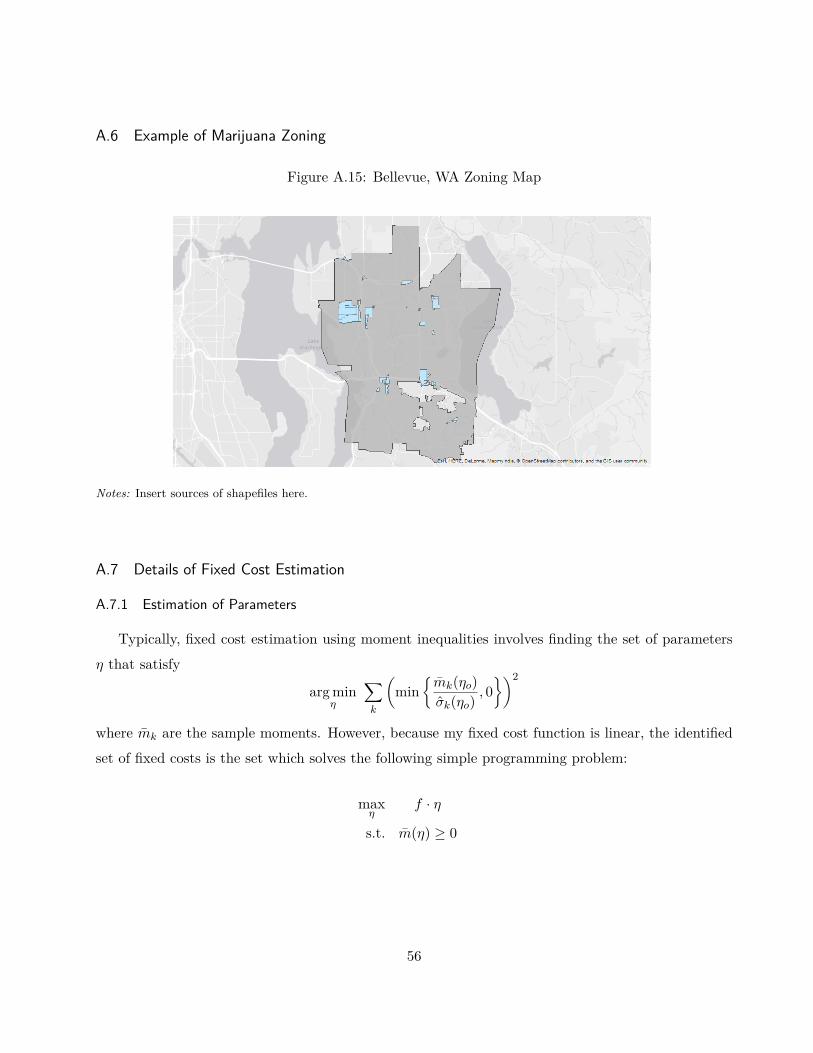
due to the reluctance of landlords to lease to marijuana businesses due to its federal illegality. In an interview a retailerdetailed the difficulties of finding a location, describing himself as “lucky” to find a good location. Figure A.15 displaysa map of marijuana retailer location constraints for the city of Bellevue, WA after accounting for local zoning ordinancesand state-mandated entry barriers.
7
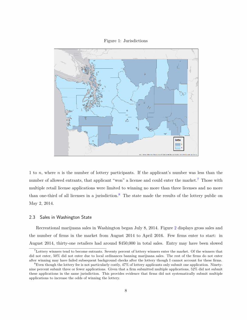
Figure 1: Jurisdictions
1 to n, where n is the number of lottery participants. If the applicant’s number was less than the
number of allowed entrants, that applicant “won” a license and could enter the market.7 Those with
multiple retail license applications were limited to winning no more than three licenses and no more
than one-third of all licenses in a jurisdiction.8 The state made the results of the lottery public on
May 2, 2014.
2.3 Sales in Washington State
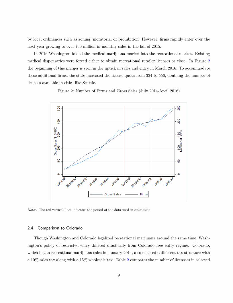
Recreational marijuana sales in Washington began July 8, 2014. Figure 2 displays gross sales and
the number of firms in the market from August 2014 to April 2016. Few firms enter to start: in
August 2014, thirty-one retailers had around $450,000 in total sales. Entry may have been slowed7Lottery winners tend to become entrants. Seventy percent of lottery winners enter the market. Of the winners that
did not enter, 50% did not enter due to local ordinances banning marijuana sales. The rest of the firms do not enterafter winning may have failed subsequent background checks after the lottery though I cannot account for these firms.
8Even though the lottery fee is not particularly costly, 47% of lottery applicants only submit one application. Ninety-nine percent submit three or fewer applications. Given that a firm submitted multiple applications, 52% did not submitthese applications in the same jurisdiction. This provides evidence that firms did not systematically submit multipleapplications to increase the odds of winning the lottery.
8
by local ordinances such as zoning, moratoria, or prohibition. However, firms rapidly enter over the
next year growing to over $30 million in monthly sales in the fall of 2015.
In 2016 Washington folded the medical marijuana market into the recreational market. Existing
medical dispensaries were forced either to obtain recreational retailer licenses or close. In Figure 2
the beginning of this merger is seen in the uptick in sales and entry in March 2016. To accommodate
these additional firms, the state increased the license quota from 334 to 556, doubling the number of
licenses available in cities like Seattle.
Figure 2: Number of Firms and Gross Sales (July 2014-April 2016)
Notes: The red vertical lines indicates the period of the data used in estimation.
2.4 Comparison to Colorado
Though Washington and Colorado legalized recreational marijuana around the same time, Wash-
ington’s policy of restricted entry differed drastically from Colorado free entry regime. Colorado,
which began recreational marijuana sales in January 2014, also enacted a different tax structure with
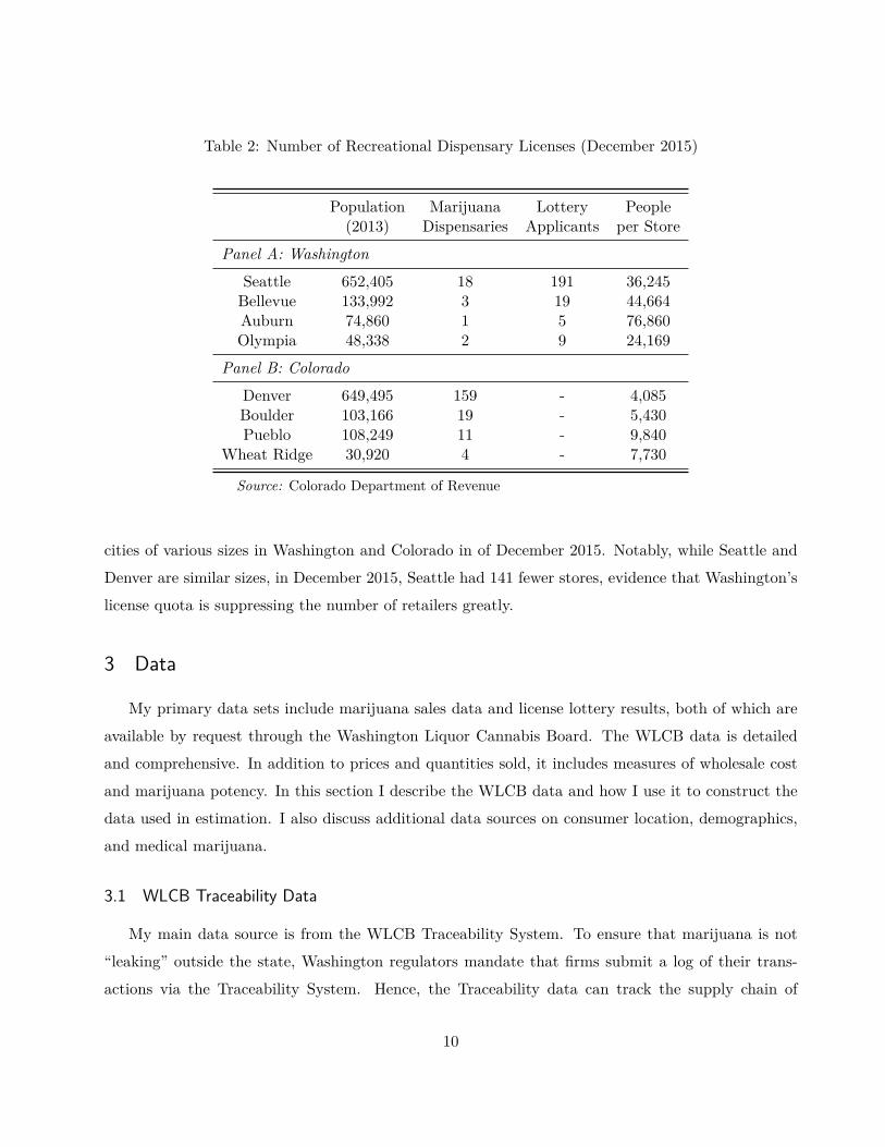
a 10% sales tax along with a 15% wholesale tax. Table 2 compares the number of licensees in selected
9
Table 2: Number of Recreational Dispensary Licenses (December 2015)
Population Marijuana Lottery People(2013) Dispensaries Applicants per Store
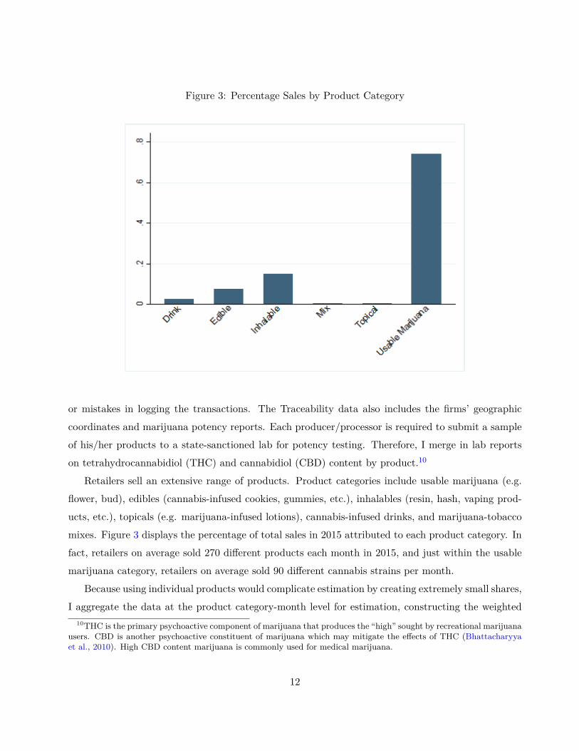
ucts, etc.), topicals (e.g. marijuana-infused lotions), cannabis-infused drinks, and marijuana-tobacco
mixes. Figure 3 displays the percentage of total sales in 2015 attributed to each product category. In
fact, retailers on average sold 270 different products each month in 2015, and just within the usable
marijuana category, retailers on average sold 90 different cannabis strains per month.
Because using individual products would complicate estimation by creating extremely small shares,
I aggregate the data at the product category-month level for estimation, constructing the weighted10THC is the primary psychoactive component of marijuana that produces the “high” sought by recreational marijuana
users. CBD is another psychoactive constituent of marijuana which may mitigate the effects of THC (Bhattacharyyaet al., 2010). High CBD content marijuana is commonly used for medical marijuana.
12
average price, wholesale cost, and median THC and CBD content for each product-store pair by
month. I also use only the top three product types—usable marijuana, inhalables and edibles—as
the market shares of topicals, drinks, and mixes are extremely small. Further, the top three product
types are sold by all firms and comprise over 96.5% of sales in Washington.11
I also limit the data to July 2015-December 2015 to avoid using data on the early recreational
market. As seen in Figure 2, in the early period after legalization, firms are entering rapidly, and
sales are quickly increasing. Using early post-legalization data would be inconsistent with a static
entry model which assumes the market is in long-run equilibrium. Further, I drop data from a firm’s
first month of sales if they are not in the market for the full month. I also exclude data after 2015
due to the entry of medical dispensaries into the recreational marijuana market at the beginning of
2016.12
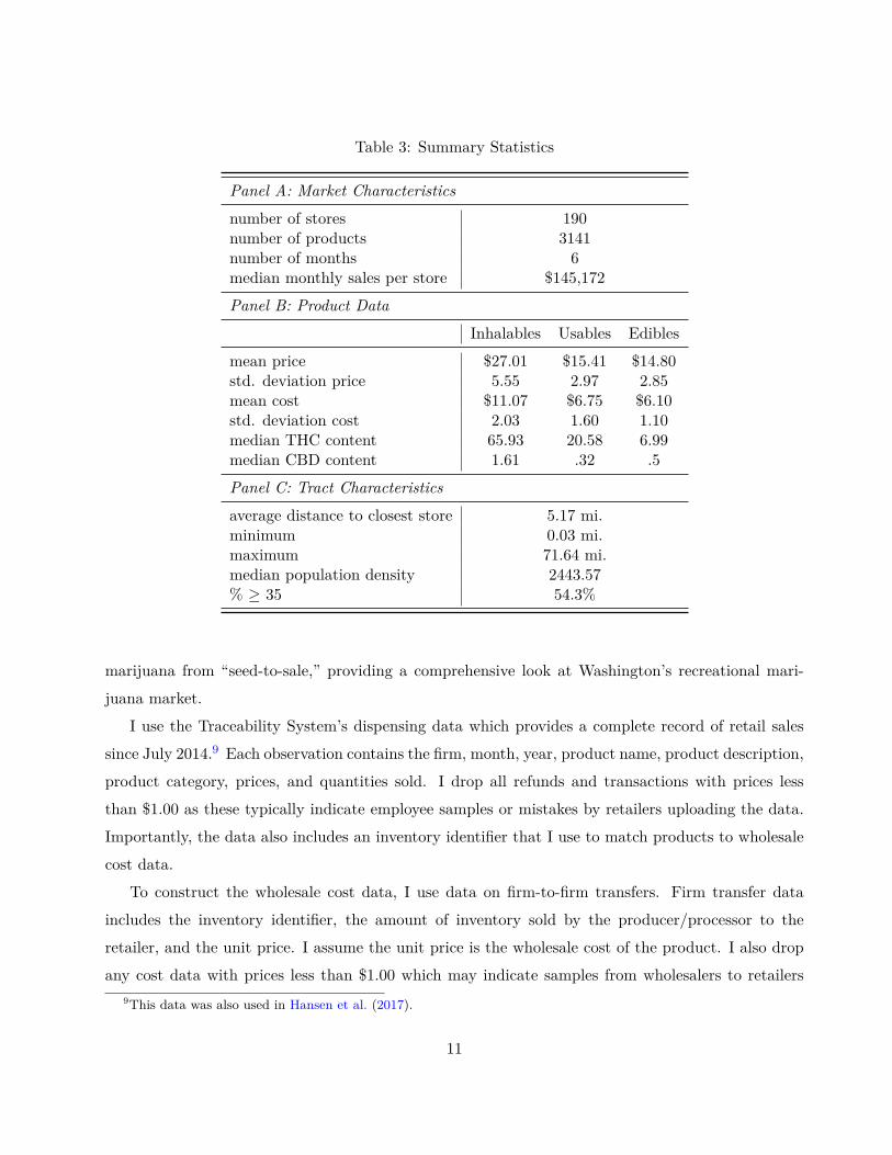
Panel A and B of Table 3 displays summary statistics of the demand data. After cleaning and
collapsing the data, I have 3,141 products for 190 individual stores over six months. Further, each
store sells usable marijuana, inhalables, and edibles. Inhalables tend to have the highest prices, and
costs and extremely high potency. Edibles, in constrast, are very low potency products though their
prices and costs are similar to usable marijuana products.
3.2 Additional WLCB Data
Additional data from the WLCB includes each jurisdictions’ license quotas and lottery results.
The lottery data includes the application number, firm tradename, and potential addresses for all
1,173 lottery entrants. Some applications list the same address, so I drop duplicate addresses. I
also drop addresses from jurisdictions with local ordinances banning retailers leaving 746 locations.
I geocode the remaining address data using Texas A&M University GeoServices, and I match the
lottery data to existing retailers.
3.3 Census Data
I proxy for consumer location by using population-weighted Washington census tract centroids
from the U.S. Census Bureau. I combine this data with geocoded lottery addresses and retailer data
to calculate the distances from census tracts to existing retailers and lottery losers. Panel C of Table11For 98% of stores, these products count for over 90% of all sales.12Discussions with industry professions revealed that the decision to allow medical dispensaries to enter the recreational
market was an unexpected policy change.
13
3 summarizes the distance from a tract centroid to its closest existing retailer. Stores are relatively
close to consumers—the average distance to the nearest store is less than 5.5 miles.
Furthermore, I merge the location information with demographic data and additional geographic
data found in the Census TIGER/Line shapefiles with American Community Survey (2010-2014). I
compute the total population of adults over the age of twenty-one, and as Azofeifa et al. (2016) show
that most marijuana users are below the age of 35, I also calculate the percentage of adults over the
age of thirty-five and the population density of each census tract to include in the demand model.
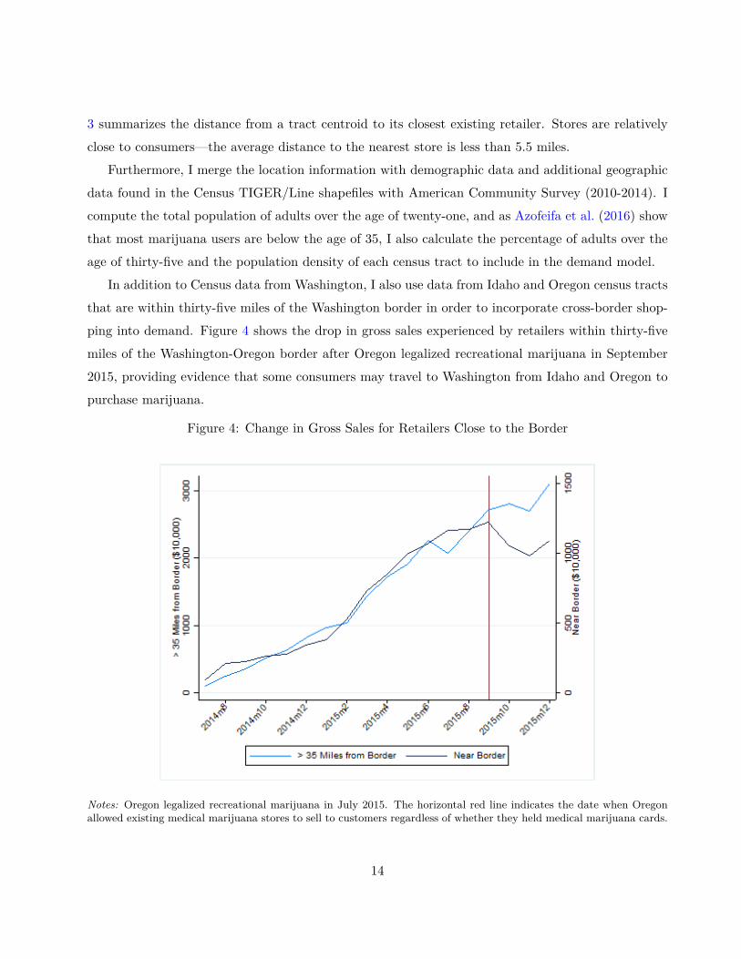
In addition to Census data from Washington, I also use data from Idaho and Oregon census tracts
that are within thirty-five miles of the Washington border in order to incorporate cross-border shop-
ping into demand. Figure 4 shows the drop in gross sales experienced by retailers within thirty-five
miles of the Washington-Oregon border after Oregon legalized recreational marijuana in September
2015, providing evidence that some consumers may travel to Washington from Idaho and Oregon to
purchase marijuana.
Figure 4: Change in Gross Sales for Retailers Close to the Border
Notes: Oregon legalized recreational marijuana in July 2015. The horizontal red line indicates the date when Oregonallowed existing medical marijuana stores to sell to customers regardless of whether they held medical marijuana cards.
14
3.4 Medical Marijuana Data
Because medical dispensaries were not regulated by the WLCB during my period of study, medical
marijuana dispensing data is not available. Nonetheless, I proxy for the existence of medical marijuana
stores using the number of medical dispensaries within ten miles of a census tract. In the demand
model, I include this information in consumers’ outside option. I obtain this address information
from the web.
A concern is that medical marijuana is a close substitute for recreational marijuana and not
including medical marijuana dispensaries will understate the amount of competition in the market.
Many untaxed and unregulated medical dispensaries and collective gardens were operating both
before and after the passage of I-502. However, my discussions with recreational retailers revealed
that I-502 retailers did not consider medical dispensaries direct competitors. Reasons included the
substantive differences in products and stores, the fact that customers did not need to obtain a
doctor’s recommendation, and the additional legitimacy provided by being state-sanctioned.
4 A Three Stage Model of Entry
I develop a three stage model that endogenizes firms’ entry decisions. The model’s timing is as
follows:
Stage 1a (Entry) – Firms make simultaneous decisions to enter a license lottery in a juris-
diction where the government has set a quota of n firms. The information set includes all
own-characteristics, characteristics of potential entrants, and license quotas.
Stage 1b (Lotto) – If there are more than n applicants, the government chooses n entrants
randomly.
Stage 2 – Firms select prices by playing a Nash-pricing game.
Stage 3 – Demand and profits are realized.
The model is solved by backwards induction; therefore, exposition of the model begins with the stage
3.
15
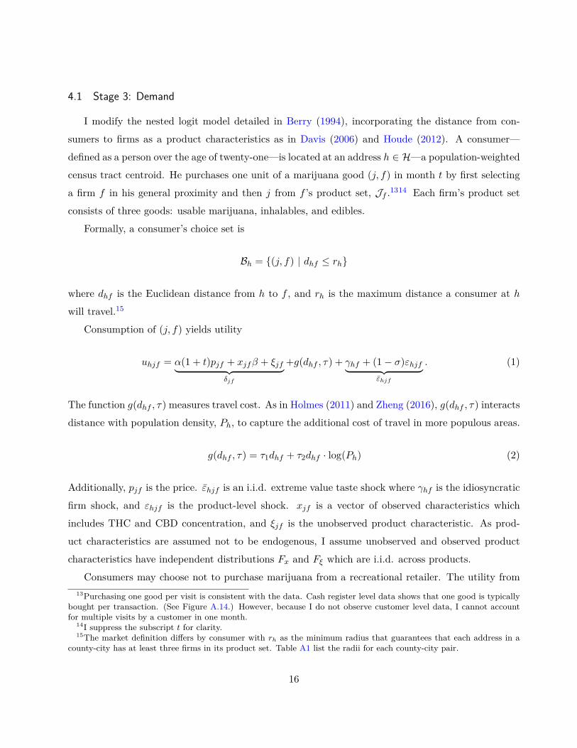
4.1 Stage 3: Demand
I modify the nested logit model detailed in Berry (1994), incorporating the distance from con-
sumers to firms as a product characteristics as in Davis (2006) and Houde (2012). A consumer—
defined as a person over the age of twenty-one—is located at an address h ∈ H—a population-weighted
census tract centroid. He purchases one unit of a marijuana good (j, f) in month t by first selecting
a firm f in his general proximity and then j from f ’s product set, Jf .1314 Each firm’s product set
consists of three goods: usable marijuana, inhalables, and edibles.
Formally, a consumer’s choice set is
Bh = {(j, f) | dhf ≤ rh}
where dhf is the Euclidean distance from h to f , and rh is the maximum distance a consumer at h
will travel.15
Consumption of (j, f) yields utility
uhjf = α(1 + t)pjf + xjfβ + ξjf︸ ︷︷ ︸δjf
+g(dhf , τ) + γhf + (1− σ)εhjf︸ ︷︷ ︸εhjf
. (1)
The function g(dhf , τ) measures travel cost. As in Holmes (2011) and Zheng (2016), g(dhf , τ) interacts
distance with population density, Ph, to capture the additional cost of travel in more populous areas.
g(dhf , τ) = τ1dhf + τ2dhf · log(Ph) (2)
Additionally, pjf is the price. εhjf is an i.i.d. extreme value taste shock where γhf is the idiosyncratic
firm shock, and εhjf is the product-level shock. xjf is a vector of observed characteristics which
includes THC and CBD concentration, and ξjf is the unobserved product characteristic. As prod-
uct characteristics are assumed not to be endogenous, I assume unobserved and observed product
characteristics have independent distributions Fx and Fξ which are i.i.d. across products.
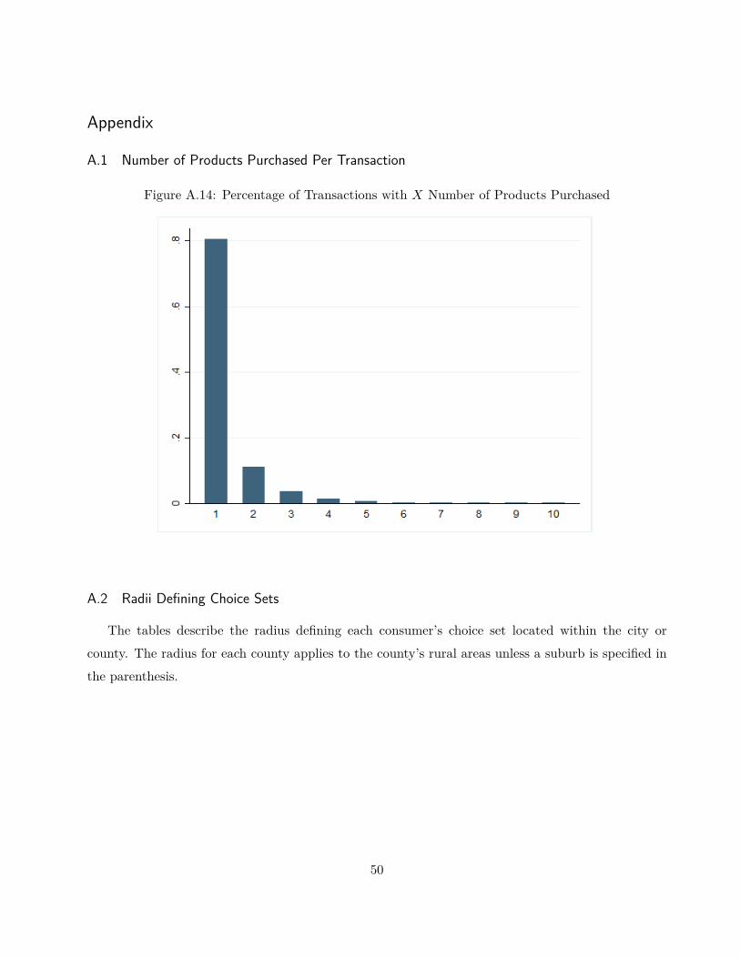
Consumers may choose not to purchase marijuana from a recreational retailer. The utility from13Purchasing one good per visit is consistent with the data. Cash register level data shows that one good is typically
bought per transaction. (See Figure A.14.) However, because I do not observe customer level data, I cannot accountfor multiple visits by a customer in one month.
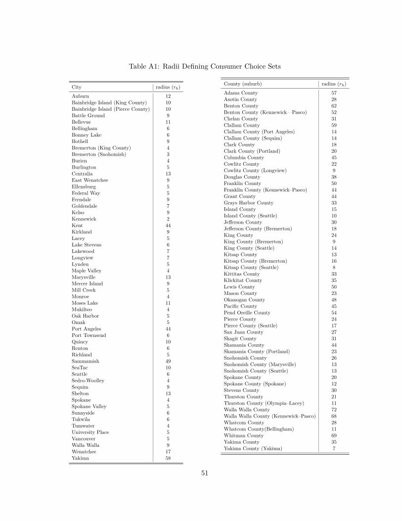
14I suppress the subscript t for clarity.15The market definition differs by consumer with rh as the minimum radius that guarantees that each address in a
county-city has at least three firms in its product set. Table A1 list the radii for each county-city pair.
16
the outside option is
uh0 = ΠDh + γh0 + εh0 (3)
where γh0 is normalized to zero. Dh is a vector of address characteristics which includes the percentage
of h’s population over the age of thirty-five and the number of medical marijuana stores within ten
miles of h in Dh.16
Consumers at h maximize their utility, choosing to purchase (j, f) with probability
shjf = shjf |f · shf ,
the product of the probability of selecting j given f and the probability of selecting f . These proba-
bilities have the standard logit forms
shjf |f = exp (δjf/(1− σ))∑j′∈Jf
exp(δj′f/(1− σ)
) (4)
shft = exp(g(dhf , τ) + (1− σ)IVf )exp(ΠDh) +
∑f ′ exp(g(dhf ′ , τ) + (1− σ)IVf ′)
(5)
with inclusive value
IVf = ln
∑j′∈Jf
exp(δj′f/(1− σ)
) .Total demand at h for (j, f) is the product of the choice probability and Mh, the number of consumers
at h. Hence, total demand is
Qjf =∑h∈Hf
shjf ·Mh. (6)
where the set Hf = {h|f ∈ Bh}, the tracts that have firm f in their choice set.
4.2 Stage 2: Pricing
Firms’ second stage decision is to set prices. Because Washington state limits the number of retail
licenses a firm can obtain, I assume a firm is single store enterprise that chooses its prices to maximize16Azofeifa et al. (2016) analyzes survey responses in the National Survey of Drug Usage and Health and finds that
people under thirty-five are primary users of marijuana. The study also finds that males are the most prevalent usersof marijuana; however, I cannot identify coefficients on gender as census tracts are all roughly fifty percent male.
17
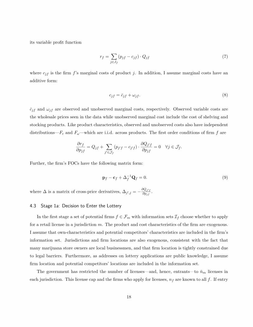
its variable profit function
rf =∑j∈Jf
(pjf − cjf ) ·Qjf (7)
where cjf is the firm f ’s marginal costs of product j. In addition, I assume marginal costs have an
additive form:
cjf = cjf + ωjf . (8)
cjf and ωjf are observed and unobserved marginal costs, respectively. Observed variable costs are
the wholesale prices seen in the data while unobserved marginal cost include the cost of shelving and
stocking products. Like product characteristics, observed and unobserved costs also have independent
distributions—Fc and Fω—which are i.i.d. across products. The first order conditions of firm f are
∂rf∂pjf
= Qjf +∑j′∈Jf
(pj′f − cj′f ) · ∂Qj′f
∂pjf= 0 ∀j ∈ Jf .
Further, the firm’s FOCs have the following matrix form:
pf − cf + ∆−1f Qf = 0. (9)
where ∆ is a matrix of cross-price derivatives, ∆j′,j = −∂Qj′f∂pjf
.
4.3 Stage 1a: Decision to Enter the Lottery
In the first stage a set of potential firms f ∈ Fm with information sets If choose whether to apply
for a retail license in a jurisdiction m. The product and cost characteristics of the firm are exogenous.
I assume that own-characteristics and potential competitors’ characteristics are included in the firm’s
information set. Jurisdictions and firm locations are also exogenous, consistent with the fact that
many marijuana store owners are local businessmen, and that firm location is tightly constrained due
to legal barriers. Furthermore, as addresses on lottery applications are public knowledge, I assume
firm location and potential competitors’ locations are included in the information set.
The government has restricted the number of licenses—and, hence, entrants—to nm licenses in
each jurisdiction. This license cap and the firms who apply for licenses, nf are known to all f . If entry
18
is constrained, nf > nm, the government chooses license recipients randomly while if nf ≤ nm, all
applicants are granted retail licenses. I assume that if f is a license recipient, f enters in jurisdiction
m.
Firms know their own product sets Jf and predict which other firms will enter the lottery though
the identities of these firms are selected by the lottery. I assume firms make their lottery entry decision
based on expected profits given the other firms who enter subsequently with the lottery. Moreover,
firms enter only if expected profits are weakly greater than zero whatever the subset of competitors
after the lottery. This implies the following inequality:
E(πf (df , d−f ; θ) | If ) ≥ 0. (10)
The profit function πf (df , d−f ; θ) has the form
πf (df , d−f ; θ) = rf (df , d−f ; θ)− F (11)
where rf (·) is equation 7, the variable profit function .
To capture higher fixed costs in urban areas, I model fixed costs as follows:
F = η1 + η2I(urbanf ). (12)
I(urban) equals one if the firm is in a urban area to capture any additional costs associated locating
in an urban area. To define urban versus rural, I use the U.S. Census definition of an “urbanized
area” which is a geographic area with “50,000 or more people.”17
5 Estimation
Estimation mirrors the logic of the backwards induction solution of the model: I estimate demand
and marginal costs yielding a measure of variable profits. I then use the estimates for variable profits
to find the fixed cost of entry.17See ”2010 Census Urban and Rural Classification and Urban Area Criteria,” United States Census Bureau,
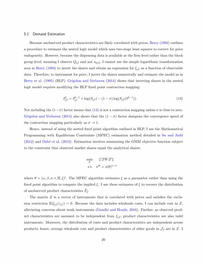
Not including the (1−σ) factor means that (13) is not a contraction mapping unless σ is close to zero.
Grigolon and Verboven (2014) also shows that the (1− σ) factor dampens the convergence speed of
the contraction mapping particularly as σ → 1.
Hence, instead of using the nested fixed point algorithm outlined in BLP, I use the Mathematical
Programming with Equilibrium Constraints (MPEC) estimation method detailed in Su and Judd
(2012) and Dube et al. (2012). Estimation involves minimizing the GMM objective function subject
to the constraint that observed market shares equal the analytical shares:
minθ
ξ′ZWZ ′ξ
s.t. sob = s(θ)1−σ
where θ = (α, β, σ, τ,Π, ξ)′. The MPEC algorithm estimates ξ as a parameter rather than using the
fixed point algorithm to compute the implied ξ. I use these estimates of ξ to recover the distribution
of unobserved product characteristics Fξ.
The matrix Z is a vector of instruments that is correlated with prices and satisfies the exclu-
sion restriction E(ξjf |zjf ) = 0. Because the data includes wholesale costs, I can include cost in Z,
alleviating concerns about weak instruments (Gandhi and Houde, 2016). Further, as observed prod-
uct characteristics are assumed to be independent from ξjf , product characteristics are also valid
instruments. Moreover, the distribution of costs and product characteristics are independent across
products; hence, average wholesale cost and product characteristics of other goods in Jf are in Z. I
20
also include the population-weighted average tract characteristics and BLP instruments—mean costs
and product characteristics of expected competitors.
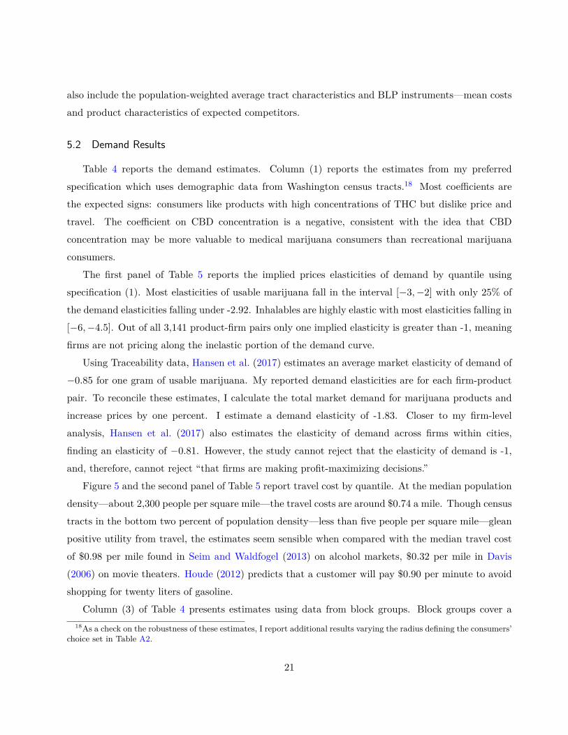
5.2 Demand Results
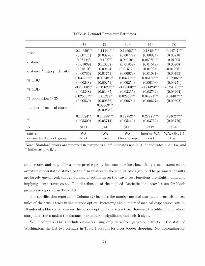
Table 4 reports the demand estimates. Column (1) reports the estimates from my preferred
specification which uses demographic data from Washington census tracts.18 Most coefficients are
the expected signs: consumers like products with high concentrations of THC but dislike price and
travel. The coefficient on CBD concentration is a negative, consistent with the idea that CBD
concentration may be more valuable to medical marijuana consumers than recreational marijuana
consumers.
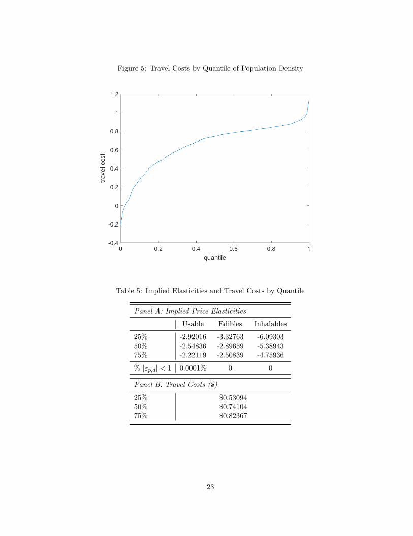
The first panel of Table 5 reports the implied prices elasticities of demand by quantile using
specification (1). Most elasticities of usable marijuana fall in the interval [−3,−2] with only 25% of
the demand elasticities falling under -2.92. Inhalables are highly elastic with most elasticities falling in
[−6,−4.5]. Out of all 3,141 product-firm pairs only one implied elasticity is greater than -1, meaning
firms are not pricing along the inelastic portion of the demand curve.
Using Traceability data, Hansen et al. (2017) estimates an average market elasticity of demand of
−0.85 for one gram of usable marijuana. My reported demand elasticities are for each firm-product
pair. To reconcile these estimates, I calculate the total market demand for marijuana products and
increase prices by one percent. I estimate a demand elasticity of -1.83. Closer to my firm-level
analysis, Hansen et al. (2017) also estimates the elasticity of demand across firms within cities,
finding an elasticity of −0.81. However, the study cannot reject that the elasticity of demand is -1,
and, therefore, cannot reject “that firms are making profit-maximizing decisions.”
Figure 5 and the second panel of Table 5 report travel cost by quantile. At the median population
density—about 2,300 people per square mile—the travel costs are around $0.74 a mile. Though census
tracts in the bottom two percent of population density—less than five people per square mile—glean
positive utility from travel, the estimates seem sensible when compared with the median travel cost
of $0.98 per mile found in Seim and Waldfogel (2013) on alcohol markets, $0.32 per mile in Davis
(2006) on movie theaters. Houde (2012) predicts that a customer will pay $0.90 per minute to avoid
shopping for twenty liters of gasoline.
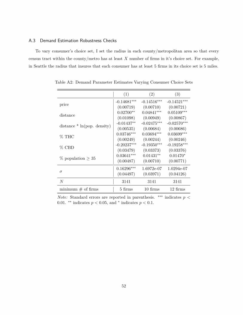
Column (3) of Table 4 presents estimates using data from block groups. Block groups cover a18As a check on the robustness of these estimates, I report additional results varying the radius defining the consumers’
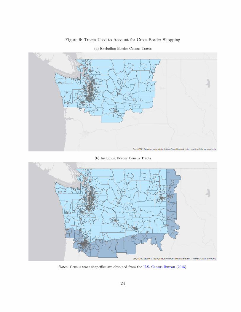
Figure 6: Tracts Used to Account for Cross-Border Shopping
(a) Excluding Border Census Tracts
(b) Including Border Census Tracts
Notes: Census tract shapefiles are obtained from the U.S. Census Bureau (2015).
24
border-crossing could overstate the size of border firms’ market shares, biasing estimates. Therefore,
I report estimates from additional specifications that account for census tracts near the Washington
state border.
Column (4) uses the interior Washington tracts, excluding tracts and stores less than thirty-five
miles from the border. Column (5) include tracts from Oregon and Idaho within thirty-five miles
of the Washigton state border. Figure 6 displays maps of the tracts used in column (4) and (5),
respectively. The coefficient estimates on price and THC are robust particularly when using census
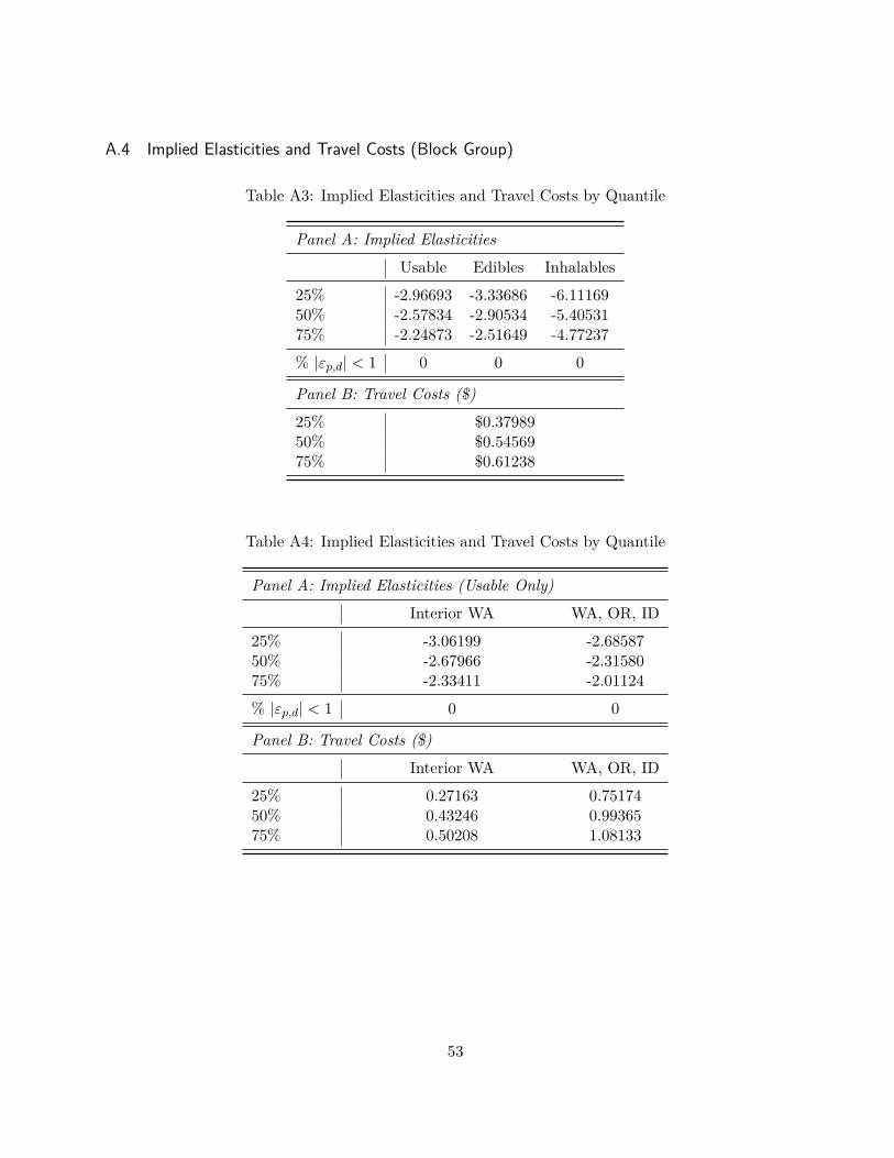
tracts from Oregon and Idaho. I report travel costs along with implied elasticities in Table A4.
Unsurprisingly, adding cross-border shoppers from Idaho and Oregon increases travel cost to $0.99
for the median population density of 2,557 people per square mile.
5.3 Marginal Cost Estimation and Results
Rather than use the Nash-pricing condition—equation (9)—to create additional moments for
demand estimation, I use the pricing equation and the demand estimates to back out unobserved
marginal costs. A similar idea is pursued in Wollman (2016) which uses the pricing equation and
demand estimates to estimate observed marginal cost parameters via least squares and then obtain
unobserved cost. I, however, have observed wholesale costs in the data and can use a non-parametric
approach. Plugging (8) into (9) and rearranging the equation to isolate ω yields an expression of
unobserved marginal costs as a function of prices, shares, observed costs and the demand model
parameters:
ωf = pf − cf −∆−1f (θ)Qf . (14)
Hence, inserting the estimated parameters θ into (14) recovers an estimate of the distribution of
unobserved marginal costs—Fω.
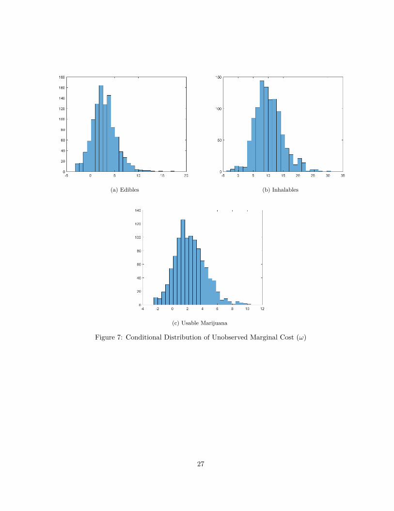
Figure 7 shows distribution of unobserved marginal costs by product. In particular, unobserved
marginal costs are generally positive, and I do not calculate that the sum of observed and unobserved
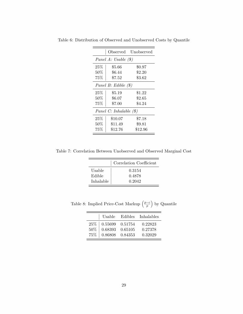
marginal cost is negative. Table 6 describes the distribution of unobserved and unobserved marginal
cost by quantile. Unobserved marginal costs for edibles and usable marijuana are generally in the
interval [0 5] in comparison to observed costs which fall in the interval [5 7]. Unobserved costs of
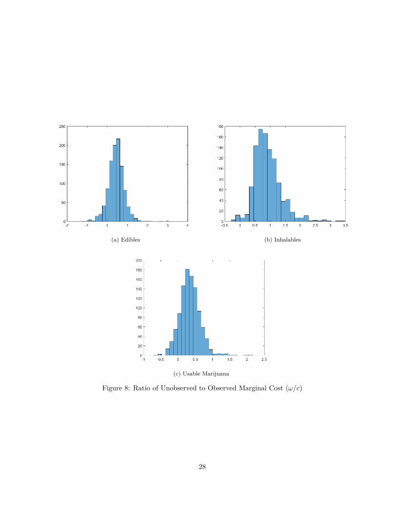
inhalables tend to be higher, falling in the interval [5 15]. Figure 8 displays the distribution of the ratio
of unobserved to observed marginal costs, providing a better picture of the magnitude of unobserved
25
versus observed marginal costs. This ratio generally falls in the interval [0,1] in all product categories,
meaning that unobserved costs do not account for a majority of variable costs. A discussion of the
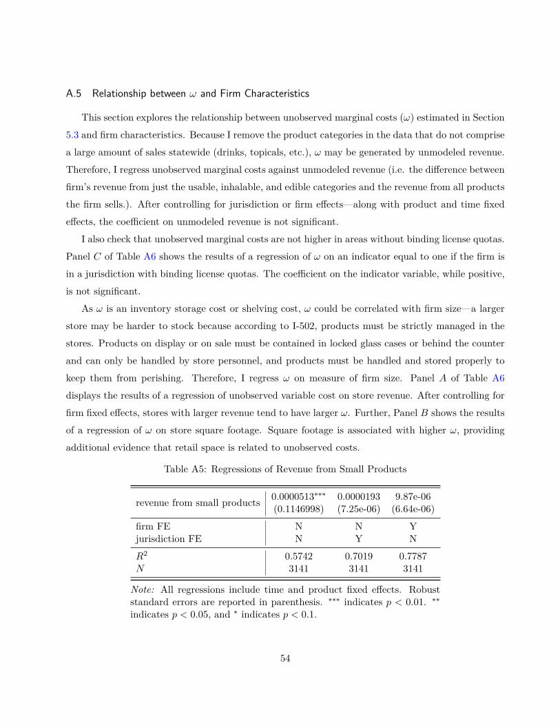
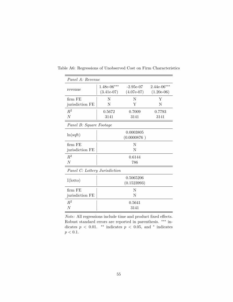
relationship between ω and firm characteristics is in Section A.5.
With cost estimates in hand, I can calculate the implied price-cost markups. Table 8 reports
the price-cost margins by quantile. The median markup on usable marijuana is 68%, slightly higher
though still in line with reports of markups of from 54-67% for one gram of usable marijuana in
Washington for 2015.19
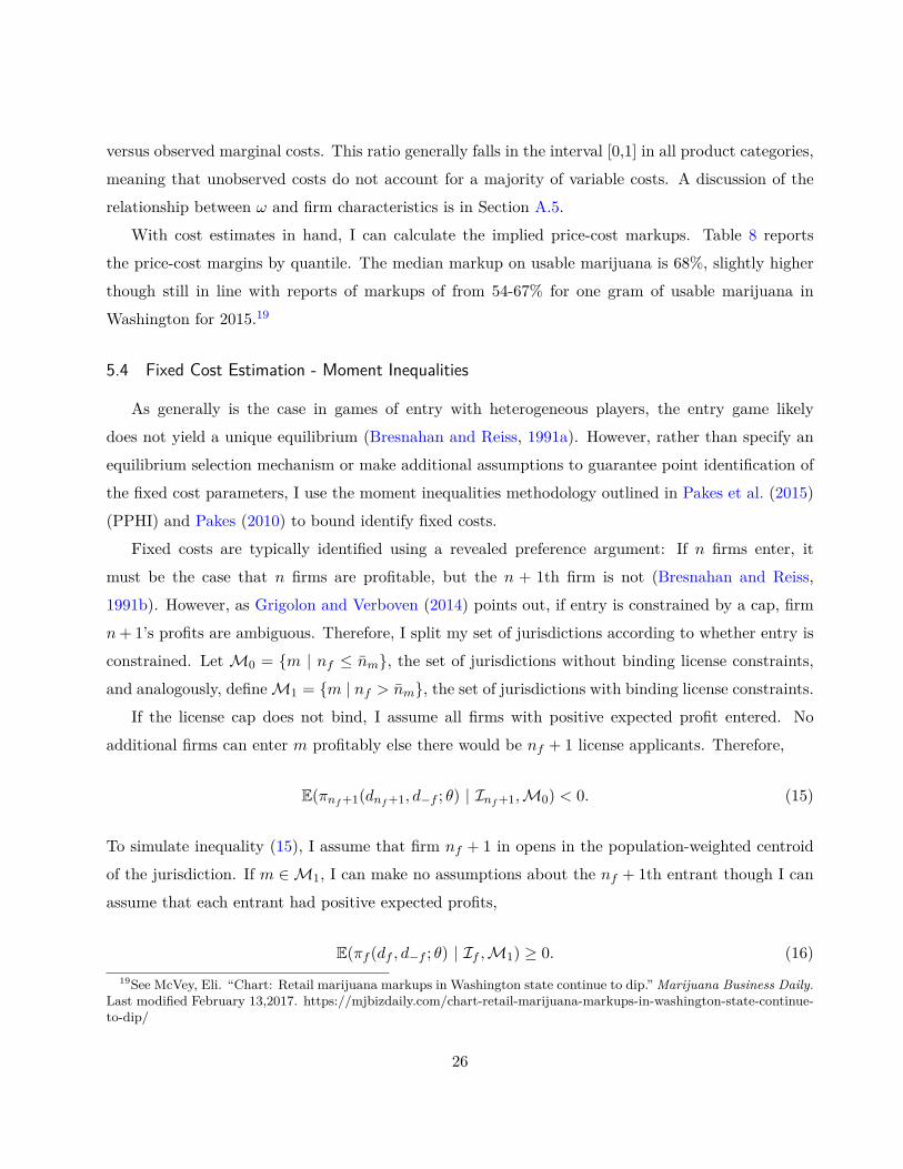
5.4 Fixed Cost Estimation - Moment Inequalities
As generally is the case in games of entry with heterogeneous players, the entry game likely
does not yield a unique equilibrium (Bresnahan and Reiss, 1991a). However, rather than specify an
equilibrium selection mechanism or make additional assumptions to guarantee point identification of
the fixed cost parameters, I use the moment inequalities methodology outlined in Pakes et al. (2015)
(PPHI) and Pakes (2010) to bound identify fixed costs.
Fixed costs are typically identified using a revealed preference argument: If n firms enter, it
must be the case that n firms are profitable, but the n + 1th firm is not (Bresnahan and Reiss,
1991b). However, as Grigolon and Verboven (2014) points out, if entry is constrained by a cap, firm
n+ 1’s profits are ambiguous. Therefore, I split my set of jurisdictions according to whether entry is
constrained. Let M0 = {m | nf ≤ nm}, the set of jurisdictions without binding license constraints,
and analogously, defineM1 = {m | nf > nm}, the set of jurisdictions with binding license constraints.
If the license cap does not bind, I assume all firms with positive expected profit entered. No
additional firms can enter m profitably else there would be nf + 1 license applicants. Therefore,
E(πnf +1(dnf +1, d−f ; θ) | Inf +1,M0) < 0. (15)
To simulate inequality (15), I assume that firm nf + 1 in opens in the population-weighted centroid
of the jurisdiction. If m ∈ M1, I can make no assumptions about the nf + 1th entrant though I can
assume that each entrant had positive expected profits,
E(πf (df , d−f ; θ) | If ,M1) ≥ 0. (16)19See McVey, Eli. “Chart: Retail marijuana markups in Washington state continue to dip.” Marijuana Business Daily.
Last modified February 13,2017. https://mjbizdaily.com/chart-retail-marijuana-markups-in-washington-state-continue-to-dip/
26
(a) Edibles (b) Inhalables
(c) Usable Marijuana
Figure 7: Conditional Distribution of Unobserved Marginal Cost (ω)
27
(a) Edibles (b) Inhalables
(c) Usable Marijuana
Figure 8: Ratio of Unobserved to Observed Marginal Cost (ω/c)
28
Table 6: Distribution of Observed and Unobserved Costs by Quantile
Observed Unobserved
Panel A: Usable ($)
25% $5.66 $0.9750% $6.44 $2.2075% $7.52 $3.62
Panel B: Edible ($)
25% $5.19 $1.2250% $6.07 $2.6575% $7.00 $4.24
Panel C: Inhalable ($)
25% $10.07 $7.1850% $11.49 $9.8175% $12.76 $12.96
Table 7: Correlation Between Unobserved and Observed Marginal Cost
νf is an expectational error E(νf | If ) = 0, and (η1, η2) are parameters to be estimated.20
The empirical analog of (16) for rural jurisdictions is
1F 0
1
∑f0
1∈F01
rf (df , d−f ; θ)− η1 > 0 (19)
where F01 is the set of firms in rural jurisdictions with binding license quotas, and F 0
1 = |F01 |. Likewise,
the empirical analog of (15) for rural jurisdictions is
1F 0
0
∑f0
0∈F00
rnf +1(dnf +1, d−f ; θ)− η1 ≤ 0. (20)
F00 is the set of firms in rural jurisdictions with without binding license quotas, and F 0
0 = |F00 |.
Therefore, the fixed cost bounds for rural jurisdictions are
1F 0
0
∑f0
0∈F00
rnf +1(dnf +1, d−f ; θ) ≤ η1 <1F 0
1
∑f0
1∈F01
rf (df , d−f ; θ) (21)
Defining the sample moments analogously for rural areas, I obtain the bounds
1F 1
0
∑f1
0∈F10
rnf +1(dnf +1, d−f ; θ) ≤ η1 + η2 <1F 1
1
∑f1
1∈F11
rf (df , d−f ; θ). (22)
Additional details on estimation such as the estimation algorithm are presented in Section A.7.1.
5.5 Fixed Cost Results
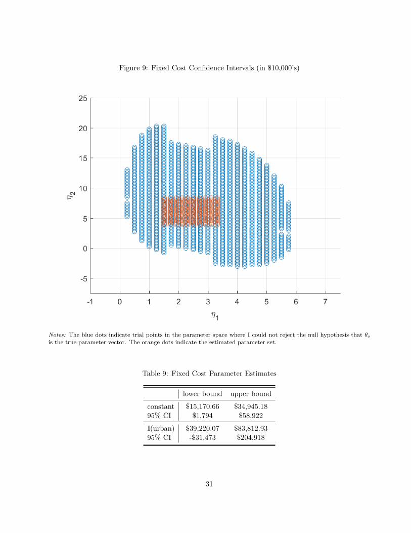
The estimates for the fixed cost parameters are reported in Table 9. The estimates imply that
urban retailers have fixed costs between $54,390 and $118,757 while rural retailers have fixed costs
between $15,170 and $34,945. These are consistent with discussions with industry professionals who20PPHI allows for a structural error term. However, I do not assume a structural error. Therefore, all heterogeneity
in fixed costs comes from whether retailers are rural or urban.
30
Figure 9: Fixed Cost Confidence Intervals (in $10,000’s)
Notes: The blue dots indicate trial points in the parameter space where I could not reject the null hypothesis that θo
is the true parameter vector. The orange dots indicate the estimated parameter set.
Table 9: Fixed Cost Parameter Estimates
lower bound upper bound
constant $15,170.66 $34,945.1895% CI $1,794 $58,922
I(urban) $39,220.07 $83,812.9395% CI -$31,473 $204,918
31
estimated that retailers in urban areas must earn around $100,000 per month to break even while
stores in rural areas can make substantially less and stay in business ($10,000-$30,000 per month).
Recent reports in the industry estimate the median annual operating costs of recreational marijuana
dispensaries to be $600,000.21
Standard errors are calculated using the asymptotic version of the Generalized Moment Section
test detailed in Andrews and Soares (2010). Additional details on calculating standard errors are
presented in Section A.7.2. Table 9 displays the projections of the 95% confidence set. However,
more informative is Figure 9 which displays the full confidence set. The confidence set is large,
unsurprising due to the small number of firms and jurisdictions. Moreover, I cannot rule out that the
parameter value for η2 is less than zero. However, as Figure 9 shows, if η2 < 0, η1 tends to be large.
Therefore, total fixed costs are always positive in the 95% confidence set. Nonetheless, I cannot reject
that urban fixed costs are less than rural fixed costs.
6 Counterfactuals
In this section I explain the computation of my counterfactual simulations and discuss the results. I
begin by exploring a policy of free entry. Free entry improves surplus relative to a baseline simulation
of Washington’s license quota policy. I then break down the sources of this gain to explore the
role of allocative efficiency by simulating the outcome of license auctions. The surplus generated
by a statewide license auction that distributes the same number of licenses as the license quota
does not have allocative costs due to either geographic license restrictions or the lottery while a
within-jurisdiction license auction that distributes the same number of licenses in a county/city incurs
allocative costs due to geographic misallocation but not due to randomization. Thus, the differences
in surplus generated by each of these simulations allow me to discuss the importance of each source
of inefficiency caused by Washington’s license quota policy.
I also discuss additional counterfactuals that directly control for the marginal damages of mari-
juana consumption. To do this, I back out the tax rates that hold marijuana/THC consumption fixed
to baseline consumption. As taxes with free entry neither restrict over geography nor keeps the most
efficient firms from entering, these policies control for negative externalities without creating alloca-
tive costs. I also explore efficiency improving tax policies assuming heterogenous marginal damages21See McVey, Eli. “Chart of the Week: Profitability in the Cannabis Industry.” Marijuana Business Daily. Last
modified May 9,2016. https://mjbizdaily.com/chart-of-the-week-profitability-in-the-cannabis-industry/
32
across geography, backing out the implied non-uniform tax schedule consistent with Washington’s
current regime of license quotas.
6.1 Unrestricted Entry Counterfactual
In the model firms entered the lottery with knowledge of the license quota and the fact that
competition will be reduced. Hence, without the quota I cannot assume that all who entered the
lottery would enter the market. In the unrestricted entry scenario, I assume that all lottery entrants
in the data are potential entrants in the free entry game and use the associated lottery addresses as
their locations. (I draw from the empirical distributions of Fx, Fη, Fc, and Fω to simulate the firm
characteristics of lottery losers.) As before, firms are still endowed with their locations, products,
and costs, and these are known to all competitors. However, now there is no lottery randomization.
Firms enter if expected profits are positive:
E(π(di, d−i, θ)|If ) ≥ 0.
6.1.1 Computing Counterfactual Entry
Multiple equilibria are almost certain in an entry game with heterogeneous firms. Therefore, to
compute counterfactual entry with tax t, I adopt an iterative best response process similar to Wollman
(2016).22 I begin by assuming all n potential entrants have entered, d = 1, and specifying an order in
which firms make their decisions, ordering by profitability. Assuming a tax of t, I play a Nash-pricing
game with all n firms. I then allow firm 1 to play its best response: enter or not enter. The firms in
the market then replay the Nash-pricing game. Next, firm 2 plays its best response given the actions
of the other players, and the Nash-pricing game is replayed based on firm 2’s choice. This continues
until I go through each firm in the order. I repeat this process until I converge to a solution where
all entrants have positive expected profits, and no firm has a profitable deviation.
6.1.2 Computing Baseline Entry
In the unrestricted entry game described in Section , firms know their competitors and competitors’
characteristics, and there is no lottery randomization. Hence, under free entry there is no ex-post
regret. However, due expectational error, firms in the entry model described in Section 4.3 and may22Lee and Pakes (2009) also discuss the equilibrium selection, suggesting learning processes which “select out” equi-
libria.
33
experience ex-post regret. To bring consistency between the two simulations, I compute the baseline
simulation by first randomly ordering firms within each jurisdiction as described in Section 2.2. I
then take the first n firms in each jurisdiction as the lottery winners. All lottery winners enter the
market. If a firm experiences ex-post regret, I remove that firm and replace it with the next firm in
the lottery ordering. I do this until all firms have positive profits. Guaranteeing that all firms in the
baseline simulation have no ex-post regret increases the magnitude of total surplus, consumer surplus,
producer surplus, and tax revenue though fixed costs are constant. This biases the results away from
finding inefficiency due to license allocation and, thus, does not greatly impact the interpretation of
the results.
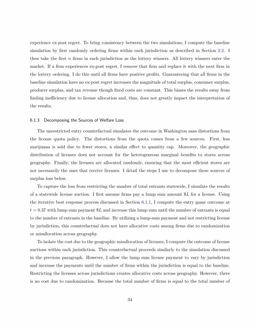
6.1.3 Decomposing the Sources of Welfare Loss
The unrestricted entry counterfactual simulates the outcome in Washington sans distortions from
the license quota policy. The distortions from the quota comes from a few sources. First, less
marijuana is sold due to fewer stores, a similar effect to quantity cap. Moreover, the geographic
distribution of licenses does not account for the heterogeneous marginal benefits to stores across
geography. Finally, the licenses are allocated randomly, ensuring that the most efficient stores are
not necessarily the ones that receive licenses. I detail the steps I use to decompose these sources of
surplus loss below.
To capture the loss from restricting the number of total entrants statewide, I simulate the results
of a statewide license auction. I first assume firms pay a lump sum amount $L for a license. Using
the iterative best response process discussed in Section 6.1.1, I compute the entry game outcome at
t = 0.37 with lump sum payment $L and increase this lump sum until the number of entrants is equal
to the number of entrants in the baseline. By utilizing a lump-sum payment and not restricting license
by jurisdiction, this counterfactual does not have allocative costs among firms due to randomization
or misallocation across geography.
To isolate the cost due to the geographic misallocation of licenses, I compute the outcome of license
auctions within each jurisdiction. This counterfactual proceeds similarly to the simulation discussed
in the previous paragraph. However, I allow the lump sum license payment to vary by jurisdiction
and increase the payments until the number of firms within the jurisdiction is equal to the baseline.
Restricting the licenses across jurisdictions creates allocative costs across geography. However, there
is no cost due to randomization. Because the total number of firms is equal to the total number of
34
firms in the baseline, this simulation captures the loss from both geographic misallocation and the
restricted number of entrants.
Therefore, the difference in surplus between the unrestricted entry simulation and the statewide
auction reflects the loss due to restricting the number of entrants. The change in surplus between
the statewide license auction and the within-jurisdiction auctions measures the loss from geographic
misallocation. As the baseline simulation captures all the distortions from the license quota policy,
the loss in surplus between the jurisdiction-specific auctions and the baseline is accounted for by
randomization.
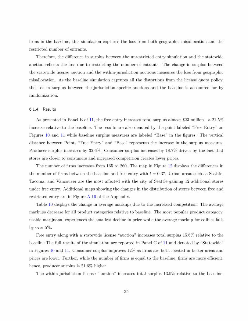
6.1.4 Results
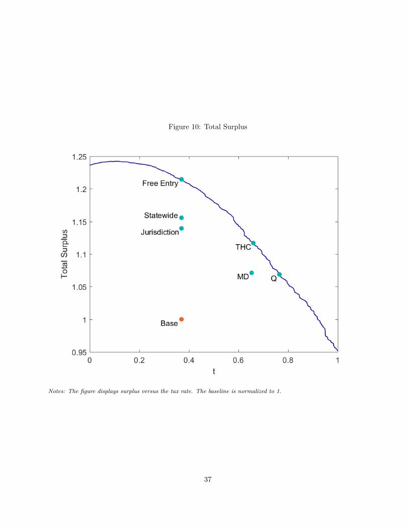
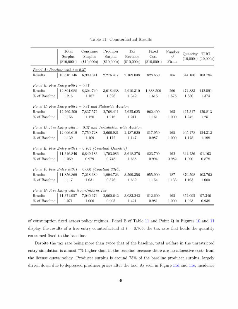
As presented in Panel B of 11, the free entry increases total surplus almost $23 million—a 21.5%
increase relative to the baseline. The results are also denoted by the point labeled “Free Entry” on
Figures 10 and 11 while baseline surplus measures are labeled “Base” in the figures. The vertical
distance between Points “Free Entry” and “Base” represents the increase in the surplus measures.
Producer surplus increases by 32.6%. Consumer surplus increases by 18.7% driven by the fact that
stores are closer to consumers and increased competition creates lower prices.
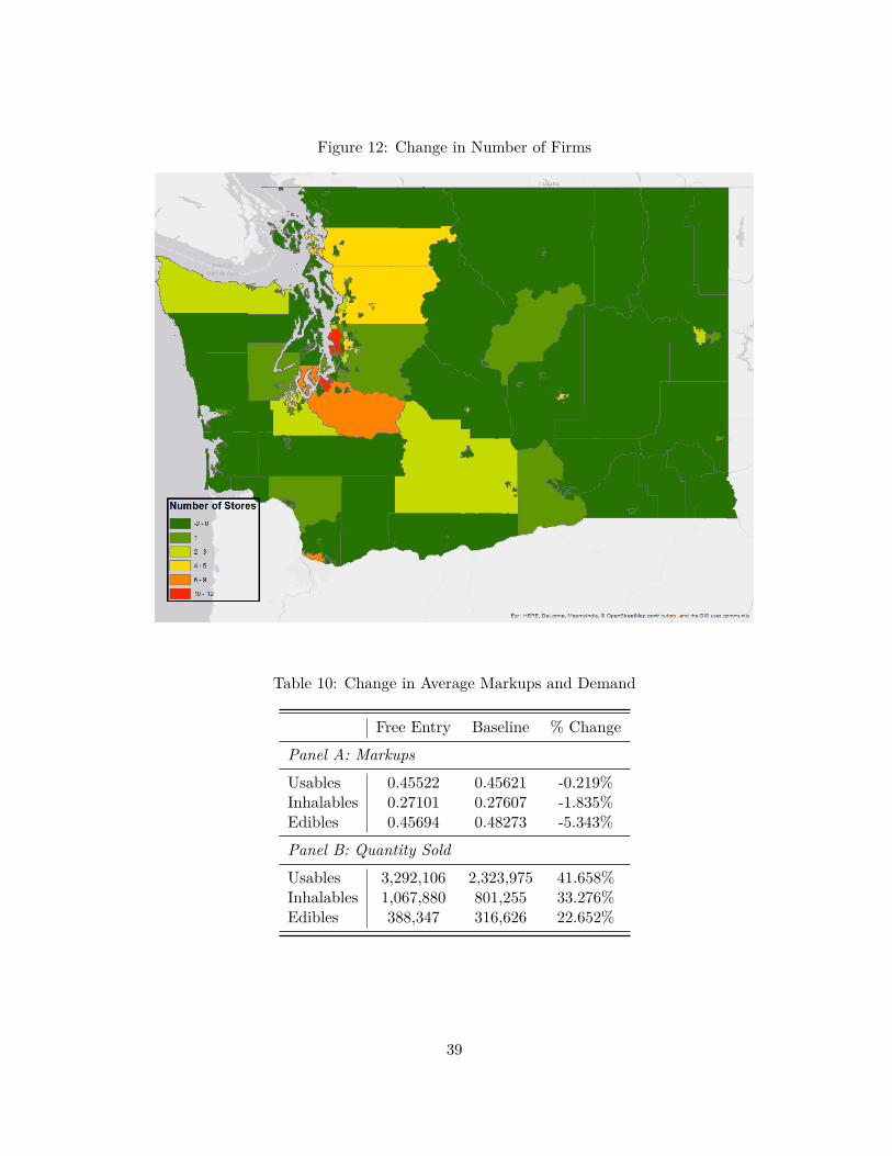
The number of firms increases from 165 to 260. The map in Figure 12 displays the differences in
the number of firms between the baseline and free entry with t = 0.37. Urban areas such as Seattle,
Tacoma, and Vancouver are the most affected with the city of Seattle gaining 12 additional stores
under free entry. Additional maps showing the changes in the distribution of stores between free and
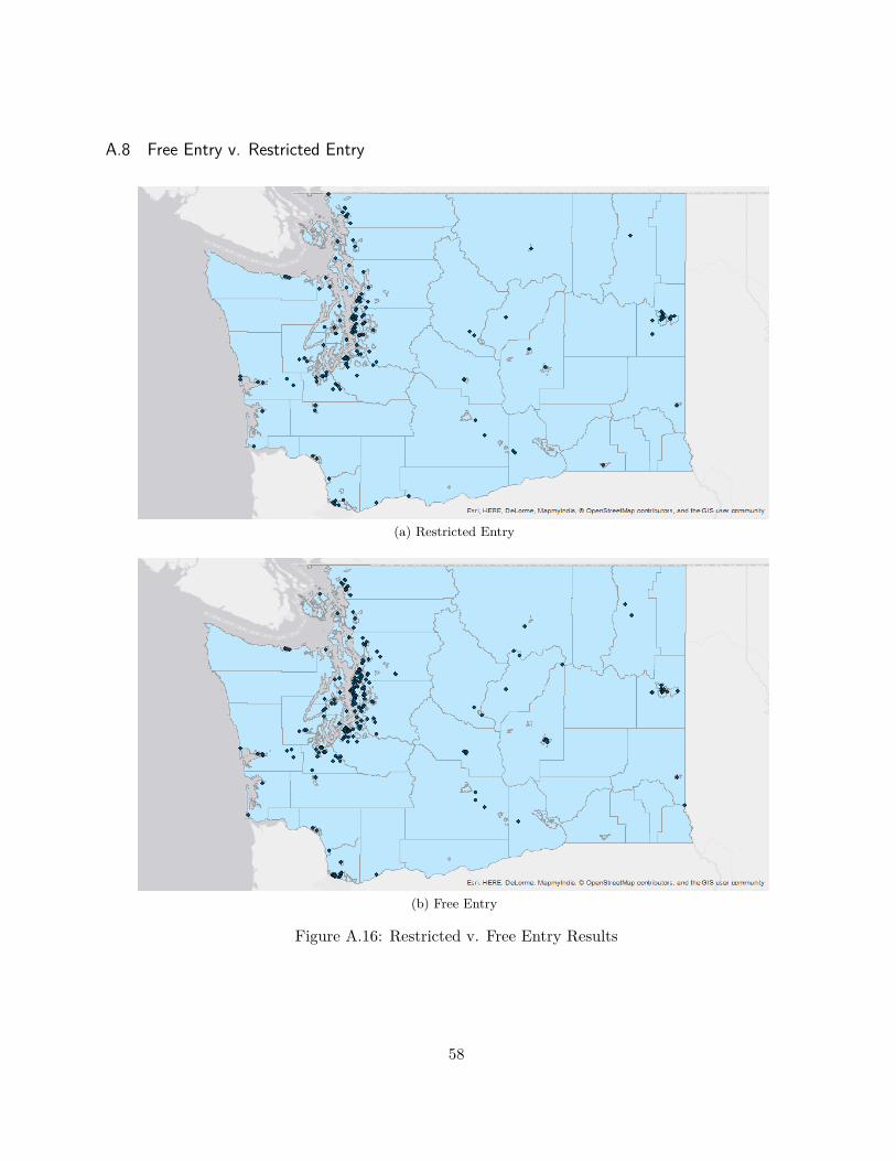
restricted entry are in Figure A.16 of the Appendix.
Table 10 displays the change in average markups due to the increased competition. The average
markups decrease for all product categories relative to baseline. The most popular product category,
usable marijuana, experiences the smallest decline in price while the average markup for edibles falls
by over 5%.
Free entry along with a statewide license “auction” increases total surplus 15.6% relative to the
baseline The full results of the simulation are reported in Panel C of 11 and denoted by “Statewide”
in Figures 10 and 11. Consumer surplus improves 12% as firms are both located in better areas and
prices are lower. Further, while the number of firms is equal to the baseline, firms are more efficient;
hence, producer surplus is 21.6% higher.
The within-jurisdiction license “auction” increases total surplus 13.9% relative to the baseline.
35
The results are reported in Panel D of 11 and denoted by “Jurisdiction” in Figures 10 and 11. Even
though the number of firms within each jurisdiction is constant, prices are still lower than in baseline.
Hence, consumers by more marijuana products, and consumer surplus increases by 10.9%. Producer
surplus is also 17.5% higher.
The cost from restricting the number of total entrants statewide, shown graphically as the vertical
distance between “Free Entry” and “Statewide” in Figure 10, comprises 27.5% of the $23 million
difference in surplus. Allocative costs constitute the remainder of the difference–over 70%. The
distance between “Statewide” and “Jurisdiction” in Figure 10 represents the cost due to geographic
misallocation, 6.6% of the change in total surplus, and the gap between “Jurisdiction” and “Baseline”
depicts the efficiency cost attributable to randomly distributing licenses to potential entrants. This
distance is the largest, representing 65.9% of the total cost.
6.2 Controlling for Marginal Damages of Consumption
Previous research in both economics and health show that marijuana causes short and long-term
cognitive impairment, impairs short-term motor function, is associated with paranoia and psychosis,
and adversely effects adolescent brain development and school performance (Crean et al., 2011; Marie
and Zolitz, 2017; Prashad and Filbey, 2017; Volkow et al., 2014). Therefore, policy makers may
institute license quotas because they care more about limiting the amount of marijuana consumed
and by extension the marginal damages of consumption.
The counterfactuals above restricted entry, controlling for marginal damages of consumption by
decreasing the number of stores. Here, I study counterfactuals that directly control for the externality
using taxation without restricting entry. Sales taxes decrease the profitability of stores, deterring firm
entry, and discourage consumption. However, unlike with Washington’s license quota, firms can enter
where they are most valuable, and firms are not randomly chosen, meaning the most efficient will enter.
Moreover, a common justification for legalizing marijuana is alleviating ailing state budgets through
a marijuana sales tax. License quotas, rather, restrict consumption without collecting revenue.
6.2.1 Controlling for Quantity Consumed
Assuming that the marginal damages of consumption are constant across products and geography
and no consumer leakage into the black market, setting taxes in an unrestricted entry regime so
that the quantity sold is the same as the baseline quantity sold should keep the marginal damages
36
Figure 10: Total Surplus
Notes: The figure displays surplus versus the tax rate. The baseline is normalized to 1.
37
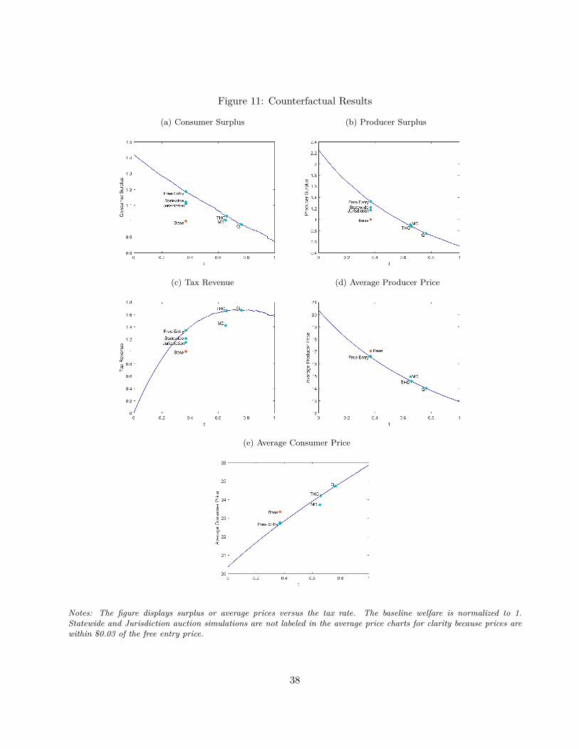
Figure 11: Counterfactual Results
(a) Consumer Surplus (b) Producer Surplus
(c) Tax Revenue (d) Average Producer Price
(e) Average Consumer Price
Notes: The figure displays surplus or average prices versus the tax rate. The baseline welfare is normalized to 1.Statewide and Jurisdiction auction simulations are not labeled in the average price charts for clarity because prices arewithin $0.03 of the free entry price.
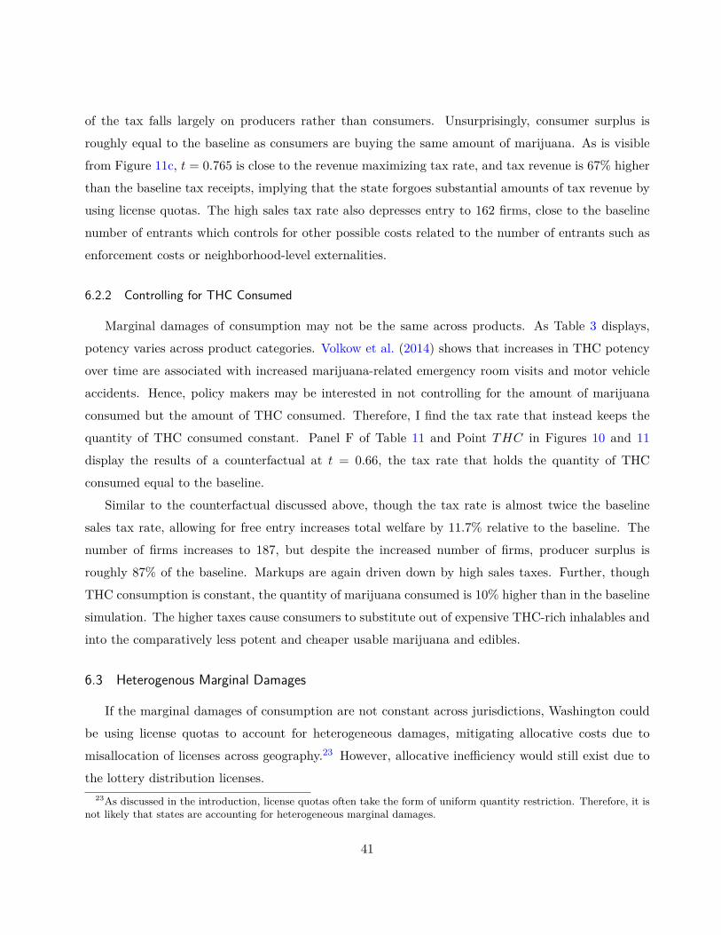
of consumption fixed across policy regimes. Panel E of Table 11 and Point Q in Figures 10 and 11
display the results of a free entry counterfactual at t = 0.765, the tax rate that holds the quantity
consumed fixed to the baseline.
Despite the tax rate being more than twice that of the baseline, total welfare in the unrestricted
entry simulation is almost 7% higher than in the baseline because there are no allocative costs from
the license quota policy. Producer surplus is around 75% of the baseline producer surplus, largely
driven down due to depressed producer prices after the tax. As seen in Figure 11d and 11e, incidence
40
of the tax falls largely on producers rather than consumers. Unsurprisingly, consumer surplus is
roughly equal to the baseline as consumers are buying the same amount of marijuana. As is visible
from Figure 11c, t = 0.765 is close to the revenue maximizing tax rate, and tax revenue is 67% higher
than the baseline tax receipts, implying that the state forgoes substantial amounts of tax revenue by
using license quotas. The high sales tax rate also depresses entry to 162 firms, close to the baseline
number of entrants which controls for other possible costs related to the number of entrants such as
enforcement costs or neighborhood-level externalities.
6.2.2 Controlling for THC Consumed
Marginal damages of consumption may not be the same across products. As Table 3 displays,
potency varies across product categories. Volkow et al. (2014) shows that increases in THC potency
over time are associated with increased marijuana-related emergency room visits and motor vehicle
accidents. Hence, policy makers may be interested in not controlling for the amount of marijuana
consumed but the amount of THC consumed. Therefore, I find the tax rate that instead keeps the
quantity of THC consumed constant. Panel F of Table 11 and Point THC in Figures 10 and 11
display the results of a counterfactual at t = 0.66, the tax rate that holds the quantity of THC
consumed equal to the baseline.
Similar to the counterfactual discussed above, though the tax rate is almost twice the baseline
sales tax rate, allowing for free entry increases total welfare by 11.7% relative to the baseline. The
number of firms increases to 187, but despite the increased number of firms, producer surplus is
roughly 87% of the baseline. Markups are again driven down by high sales taxes. Further, though
THC consumption is constant, the quantity of marijuana consumed is 10% higher than in the baseline
simulation. The higher taxes cause consumers to substitute out of expensive THC-rich inhalables and
into the comparatively less potent and cheaper usable marijuana and edibles.
6.3 Heterogenous Marginal Damages
If the marginal damages of consumption are not constant across jurisdictions, Washington could
be using license quotas to account for heterogeneous damages, mitigating allocative costs due to
misallocation of licenses across geography.23 However, allocative inefficiency would still exist due to
the lottery distribution licenses.23As discussed in the introduction, license quotas often take the form of uniform quantity restriction. Therefore, it is
not likely that states are accounting for heterogeneous marginal damages.
41
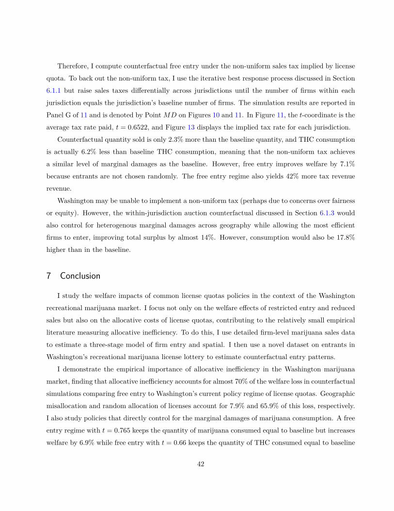
Therefore, I compute counterfactual free entry under the non-uniform sales tax implied by license
quota. To back out the non-uniform tax, I use the iterative best response process discussed in Section
6.1.1 but raise sales taxes differentially across jurisdictions until the number of firms within each
jurisdiction equals the jurisdiction’s baseline number of firms. The simulation results are reported in
Panel G of 11 and is denoted by Point MD on Figures 10 and 11. In Figure 11, the t-coordinate is the
average tax rate paid, t = 0.6522, and Figure 13 displays the implied tax rate for each jurisdiction.
Counterfactual quantity sold is only 2.3% more than the baseline quantity, and THC consumption
is actually 6.2% less than baseline THC consumption, meaning that the non-uniform tax achieves
a similar level of marginal damages as the baseline. However, free entry improves welfare by 7.1%
because entrants are not chosen randomly. The free entry regime also yields 42% more tax revenue
revenue.
Washington may be unable to implement a non-uniform tax (perhaps due to concerns over fairness
or equity). However, the within-jurisdiction auction counterfactual discussed in Section 6.1.3 would
also control for heterogenous marginal damages across geography while allowing the most efficient
firms to enter, improving total surplus by almost 14%. However, consumption would also be 17.8%
higher than in the baseline.
7 Conclusion
I study the welfare impacts of common license quotas policies in the context of the Washington
recreational marijuana market. I focus not only on the welfare effects of restricted entry and reduced
sales but also on the allocative costs of license quotas, contributing to the relatively small empirical
literature measuring allocative inefficiency. To do this, I use detailed firm-level marijuana sales data
to estimate a three-stage model of firm entry and spatial. I then use a novel dataset on entrants in
Washington’s recreational marijuana license lottery to estimate counterfactual entry patterns.
I demonstrate the empirical importance of allocative inefficiency in the Washington marijuana
market, finding that allocative inefficiency accounts for almost 70% of the welfare loss in counterfactual
simulations comparing free entry to Washington’s current policy regime of license quotas. Geographic
misallocation and random allocation of licenses account for 7.9% and 65.9% of this loss, respectively.
I also study policies that directly control for the marginal damages of marijuana consumption. A free
entry regime with t = 0.765 keeps the quantity of marijuana consumed equal to baseline but increases
welfare by 6.9% while free entry with t = 0.66 keeps the quantity of THC consumed equal to baseline
42
Figure 13: Heterogenous Sales Taxes
Notes: Map displays the non-uniform sales tax rate for each jurisdiction implied by the current policy of license quotas.
consumption but increases welfare by almost 12%. Further, assuming that license quotas are used
to account for heterogeneous marginal damages across geography, a non-uniform sales tax consistent
increases efficiency relative to the baseline by over 6%.
The magnitude of the efficiency loss and forgone tax revenue invites the question of why state
and local governments distribute licenses for “sin goods” in this manner. Possible explanations of the
license quota in itself include the limiting enforcement costs. The WLCB budget for FY2016 was 34
million dollars with 18 million allocated toward licensing and enforcement of liquor and marijuana,
a budget which is dwarfed by the increase in tax revenues in the counterfactuals. Concerns about
fairness or rent seeking could also play into distribution of licenses by lottery.
License quotas may be instruments used to control for more localized negative externalities though
quotas are not usually implemented at the neighborhood level. Thomas and Tian (2017) uses the
Washington retail license lottery as an instrument to measure the impact of marijuana dispensaries on
property values. However, research on the impact of legalized marijuana dispensaries on neighborhood
43
outcomes such as crime and hospital visits remains an fruitful area for future research.
I also leave to future research the impact of retail license quotas on upstream firms. While pro-
ducers and processors can enter the market freely in the Washington recreational marijuana market,
retailer entry restricted. Hence, producers and processors drive down their prices to compete for
highly limited shelf space in stores. Increasing the number of retailers relieves pressure on upstream
firms; hence, upstream firms may increase wholesale prices, causing an increase in retailer costs.
44
References
Adda, J., B. McConnell, and I. Rasul (2014). Crime and the Depenalization of Cannabis Possession:
Evidence from a Policing Experiment. Journal of Political Economy 122 (5), 1130–1202.
Anderson, D. M., B. Hansen, and D. I. Rees (2013). Medical Marijuana Laws, Traffic Fatalities, and
Alcohol Consumption. Journal of Law and Economics 56 (2).
Anderson, D. M., B. Hansen, and D. I. Rees (2015). Medical Marijuana Laws and Teenage Marijuana
Use. American Law and Economics Review 17 (2).
Andrews, D. W. K. and G. Soares (2010). Interence for Parameters Defined by Moment Inequalities
Using Generalized Moment Selection. Econometrica 78 (1), 119–157.
Azofeifa, A., M. E. Mattson, G. Scauer, T. McAfee, A. Grant, and R. Lyerla (2016). National
Estimates of Marijuana Use and Related Indicators – National Survey on Drug Use and Health,
United States, 2002-2014. MMWR Surveillance Summaries 65 (11).
Baumol, W. J. and W. E. Oates (1971). The Use of Standards and Prices for Protection of the
Environment. The Swedish Journal of Economics 73 (1), 42–54.
Berry, S. T. (1992). Estimation of a Model of Entry in the Airline Industry. Econometrica 60 (4),
889–917.
Berry, S. T. (1994). Estimating Discrete-Choice Models of Product Differentiation. The RAND
Journal of Economics 25 (2), 242–262.
Berry, S. T., J. Levinsohn, and A. Pakes (1995). Automobile Prices in Market Equilibrium. Econo-
metrica 63 (4), 841–890.
Berry, S. T. and J. Waldfogel (1999). Free Entry and Social Inefficiency in Radio Broadcasting.
RAND Journal of Economics 30 (3), 397–420.
Bhattacharyya, S., P. D. Morrison, P. Fusar-Poli, R. Martin-Santos, S. Borgwardt, T. Winton-Brown,
C. Nosarti, C. M. O’Carroll, M. Seal, P. Allen, M. A. Mehta, J. M. Stone, N. Tunstall, V. Giampi-
etro, S. Kapur, R. M. Murray, A. W. Zuardi, J. A. Crippa, Z. Atakan, and P. K. McGuire (2010).
Opposite Effects of ∆-9-Tetrahydrocannabinol and Cannabidiol on Human Brain Function and
Eizenberg, A. (2014). Upstream Innovation and Product Variety in the United States Home PC
Market. The Review of Economic Studies 81 (3), 1003–1045.
Ferrari, S. and F. Verboven (2010). Empirical Analysis of Markets with Free and Restricted Entry.
International Journal of Industrial Organization 28 (4), 403–406.
46
Frech, H. I. and W. C. Lee (1987). The Welfare Cost of Rationing-By-Queuing across Markets:
Theory and Estimates fromthe U.S. Gasoline Crises. The Quarterly Journal of Economics 102 (1),
97–108.
Frechette, G., A. Lizzeri, and T. Salz (2016). Frictions in a Competitive, Regulated Market: Evidence
from Taxis. Working paper.
Gandhi, A. and J.-F. Houde (2016). Measuring Substitution Patterns in Differentiated Products
Industries. Working paper.
Glaeser, E. L. and E. F. P. Luttmer (2003). The Misallocation of Housing Under Rent Control.
American Economic Review 93 (4), 1027–1046.
Glaeser, E. L. and A. Shleifer (2001). A Reason for Quantity Regulation. American Economic Review
Papers and Proceedings 91 (2), 431–435.
Grigolon, L. and F. Verboven (2014). Nested Logit or Rankdom Coefficients Logit? A Comparison
of Alternative Discrete Choice Models of Product Differentiation. The Review of Economics and
Statistics 96 (5), 916–935.
Hansen, B., K. Miller, and C. Weber (2017). The Legal Market for Marijuana: Evidence on Tax
Incidence, and the Elasticity of Demand from Washington State. Working Paper.
Holmes, T. J. (2011). The Diffusion of Wal-Mart and Economies of Density. Econometrica 79 (1),
253–302.
Houde, J.-F. H. (2012). Spatial Differentiation and Vertical Mergers in Retail Markets for Gasoline.
American Economic Review 102 (5), 2147–2482.
Jacobi, L. and M. Sovinsky (2016). Marijuana on Main Street? Estimating Demand Markets with
Limited Access. American Econmic Review 106 (8), 2009–2045.
Kaplow, L. and S. Shavell (2002). On the Superiority of Corrective Taxes to Quantity Regulation.
American Law and Economics Review 4, 1–17.
Lee, R. S. and A. Pakes (2009). Multiple Equilibria and Selection by Learning in an Applied Setting.
Economics Letters 104 (1), 13–16.
47
Luttmer, E. F. (2007). Does the Minimum Wage Cause Inefficient Rationing. The B.E. Journal of
Economic Analysis and Policy 7 (1).
Marie, O. and U. Zolitz (2017). “High” Achievers? Cannabis Access and Academic Performance.
Review of Economic Studies 84 (3), 1210–1237.
Mazzeo, M. J. (2002). Product Choice and Oligopoly Market Structure. RAND Journal of Eco-
nomics 33 (2), 221–242.
Nosko, C. (2010). Competition and Quality Choice in the CPU Market. Working Paper.
Pakes, A. (2010). Alternative Models for Moment Inequalities. Econometrica 78 (6), 1783–1822.
Pakes, A., J. Porter, K. Ho, and J. Ishii (2015). Moment Inequalities and Their Application. Econo-
metrica 83 (1), 315–334.
Prashad, S. and F. M. Filbey (2017). Cognitive Motor Deficits in Cannabis Users. Current Opinion
in Behavioral Sciences 13, 1–7.
Schaumans, C. and F. Verboven (2008). Entry and Regulation: Evidence from Health Care Profes-
sions. The RAND Journal of Economics 39 (4), 949–972.
Seim, K. (2006). An Empirical Model of Firm Entry with Endogenous Product-Type Choices. RAND
Journal of Economics 37 (3), 619–640.
Seim, K. and J. Waldfogel (2013). Public Monopoly and Economic Efficiency: Evidence from the
Pennsylvania Liquor Control Board’s Entry Decisions. American Economic Review 103 (2), 831–
862.
Su, C.-L. and K. L. Judd (2012). Constrained Optimization Approaches to Estimation of Structural
Models. Econometrica 80 (5), 2213–2230.
Thomas, D. and L. Tian (2017). Hits from the Bong? The Impact of Recreational Marijuana
Dispensaries on Property Values. Working Paper.
U.S. Census Bureau (2015). 2015 TIGER/Line Shapefiles (machine-readable data files).
Viscusi, W. K., J. Harrington, and J. Vernon. Economics of Regulation and Antitrust (4 ed.). MIT
Press.
48
Volkow, N. D., R. D. Baler, W. M. Compton, and S. R. Weiss (2014). Adverse Health Effects of
Marijuana Use. The New England Journal of Medicine 370 (23), 2219–2227.
Weitzman, M. L. (1974). Prices vs. Quantities. Review of Economic Studies 41 (4), 477–491.
Wollman, T. (2016). Trucks without Bailouts: Equilibrium Product Characteristics for Commercial
Vehicles. Working Paper.
Zheng, F. (2016). Spatial Competition and Preemptive Entry in the Discount Retail Industry. Work-
ing paper.
49
Appendix
A.1 Number of Products Purchased Per Transaction
Figure A.14: Percentage of Transactions with X Number of Products Purchased
A.2 Radii Defining Choice Sets
The tables describe the radius defining each consumer’s choice set located within the city or
county. The radius for each county applies to the county’s rural areas unless a suburb is specified in
the parenthesis.
50
Table A1: Radii Defining Consumer Choice Sets
City radius (rh)
Auburn 12Bainbridge Island (King County) 10Bainbridge Island (Pierce County) 10Battle Ground 9Bellevue 11Bellingham 6Bonney Lake 6Bothell 9Bremerton (King County) 4Bremerton (Snohomish) 3Burien 4Burlington 5Centralia 13East Wenatchee 9Ellensburg 5Federal Way 5Ferndale 9Goldendale 7Kelso 9Kennewick 2Kent 44Kirkland 9Lacey 5Lake Stevens 6Lakewood 7Longview 7Lynden 5Maple Valley 4Marysville 13Mercer Island 9Mill Creek 5Monroe 4Moses Lake 11Mukilteo 4Oak Harbor 5Omak 5Port Angeles 44Port Townsend 6Quincy 10Renton 6Richland 5Sammamish 49SeaTac 10Seattle 6Sedro-Woolley 4Sequim 9Shelton 13Spokane 4Spokane Valley 5Sunnyside 6Tukwila 6Tumwater 4University Place 5Vancouver 5Walla Walla 9Wenatchee 17Yakima 58
County (suburb) radius (rh)
Adams County 57Asotin County 28Benton County 62Benton County (Kennewick—Pasco) 52Chelan County 31Clallam County 59Clallam County (Port Angeles) 14Clallam County (Sequim) 14Clark County 18Clark County (Portland) 20Columbia County 45Cowlitz County 22Cowlitz County (Longview) 9Douglas County 38Franklin County 50Franklin County (Kennewick–Pasco) 44Grant County 44Grays Harbor County 33Island County 15Island County (Seattle) 10Jefferson County 30Jefferson County (Bremerton) 18King County 24King County (Bremerton) 9King County (Seattle) 14Kitsap County 13Kitsap County (Bremerton) 16Kitsap County (Seattle) 8Kittitas County 33Klickitat County 35Lewis County 50Mason County 23Okanogan County 48Pacific County 45Pend Oreille County 54Pierce County 24Pierce County (Seattle) 17San Juan County 27Skagit County 31Skamania County 44Skamania County (Portland) 23Snohomish County 26Snohomish County (Marysville) 13Snohomish County (Seattle) 13Spokane County 20Spokane County (Spokane) 12Stevens County 30Thurston County 21Thurston County (Olympia–Lacey) 11Walla Walla County 72Walla Walla County (Kennewick–Pasco) 68Whatcom County 28Whatcom County(Bellingham) 11Whitman County 69Yakima County 35Yakima County (Yakima) 7
51
A.3 Demand Estimation Robustness Checks
To vary consumer’s choice set, I set the radius in each county/metropolitan area so that every
census tract within the county/metro has at least X number of firms in it’s choice set. For example,
in Seattle the radius that insures that each consumer has at least 5 firms in its choice set is 5 miles.
A.5 Relationship between ω and Firm Characteristics
This section explores the relationship between unobserved marginal costs (ω) estimated in Section
5.3 and firm characteristics. Because I remove the product categories in the data that do not comprise
a large amount of sales statewide (drinks, topicals, etc.), ω may be generated by unmodeled revenue.
Therefore, I regress unobserved marginal costs against unmodeled revenue (i.e. the difference between
firm’s revenue from just the usable, inhalable, and edible categories and the revenue from all products
the firm sells.). After controlling for jurisdiction or firm effects—along with product and time fixed
effects, the coefficient on unmodeled revenue is not significant.
I also check that unobserved marginal costs are not higher in areas without binding license quotas.
Panel C of Table A6 shows the results of a regression of ω on an indicator equal to one if the firm is
in a jurisdiction with binding license quotas. The coefficient on the indicator variable, while positive,
is not significant.
As ω is an inventory storage cost or shelving cost, ω could be correlated with firm size—a larger
store may be harder to stock because according to I-502, products must be strictly managed in the
stores. Products on display or on sale must be contained in locked glass cases or behind the counter
and can only be handled by store personnel, and products must be handled and stored properly to
keep them from perishing. Therefore, I regress ω on measure of firm size. Panel A of Table A6
displays the results of a regression of unobserved variable cost on store revenue. After controlling for
firm fixed effects, stores with larger revenue tend to have larger ω. Further, Panel B shows the results
of a regression of ω on store square footage. Square footage is associated with higher ω, providing
additional evidence that retail space is related to unobserved costs.
Table A5: Regressions of Revenue from Small Products
revenue from small products 0.0000513∗∗∗ 0.0000193 9.87e-06(0.1146998) (7.25e-06) (6.64e-06)
firm FE N N Yjurisdiction FE N Y N
R2 0.5742 0.7019 0.7787N 3141 3141 3141
Note: All regressions include time and product fixed effects. Robuststandard errors are reported in parenthesis. ∗∗∗ indicates p < 0.01. ∗∗indicates p < 0.05, and ∗ indicates p < 0.1.
54
Table A6: Regressions of Unobserved Cost on Firm Characteristics
Note: All regressions include time and product fixed effects.Robust standard errors are reported in parenthesis. ∗∗∗ in-dicates p < 0.01. ∗∗ indicates p < 0.05, and ∗ indicatesp < 0.1.
55
A.6 Example of Marijuana Zoning
Figure A.15: Bellevue, WA Zoning Map
Notes: Insert sources of shapefiles here.
A.7 Details of Fixed Cost Estimation
A.7.1 Estimation of Parameters
Typically, fixed cost estimation using moment inequalities involves finding the set of parameters
η that satisfy
arg minη
∑k
(min
{mk(ηo)σk(ηo)
, 0})2
where mk are the sample moments. However, because my fixed cost function is linear, the identified
set of fixed costs is the set which solves the following simple programming problem:
maxη
f · η
s.t. m(η) ≥ 0
56
where f = {[1, 0]; [−1, 0]; [0, 1]; [0,−1]}. This programming problem is solved for every vector in f .
m(η) is a vector of sample moments defined in Section 6.1.2:
m(η) =
−(
1F 1
0
∑f1
0∈F10rnf +1(dnf +1, d−f ; θ)
)1F 1
1
∑f1
1∈F11rf (df , d−f ; θ)
−(
1F 0
0
∑f0
0∈F00rnf +1(dnf +1, d−f ; θ)
)1F 0
1
∑f0
1∈F01rf (df , d−f ; θ)
A.7.2 Calculation of Standard Errors
To compute confidence intervals, I form an evenly spaced grid, and within the grid I take a guess
of the parameter values, ηo = (η1, η2). I then find the mean and variance of the sample moments
evaluated at ηo, and compute
Qn(ηo) =∑k
(min
{mk(ηo)σk(ηo)
, 0})2
where mk(η) is moment condition k and σk(η) is the standard error of the sample moment k. The
mean and variance are normally distributed, so I then bootstrap from the empirical distribution of
the Qn. I then accept the points in the confidence set for which Qn(ηo) falls below the ninety-fifth
percentile of the bootstrapped objective function evaluations. For more specific details I refer to
Andrews and Soares (2010) and the Appendix of Dickstein and Morales (2016).