Page 1
i
Life Cycle Assessment of Ethanol produced from Lignocellulosic Biomass:
Techno-economic and Environmental Evaluation
by
Poritosh Roy
A Thesis
presented to
The University of Guelph
In partial fulfilment of requirements
for the degree of
Doctor of Philosophy
in
Engineering
Guelph, Ontario, Canada
© Poritosh Roy, August, 2014
Page 2
ii
ABSTRACT
LIFE CYCLE ASSESSMENT OF ETHANOL PRODUCED FROM LIGNOCELLULOSIC
BIOMASS: TECHNO-ECONOMIC AND ENVIRONMENTAL EVALUATION
Poritosh Roy Advisor:
University of Guelph, 2014 Dr. Animesh Dutta
The life cycle (LC) of ethanol derived from lignocellulosic biomass (hereafter referred to
biomass: wheat straw, sawdust & miscanthus) by both enzymatic hydrolysis and thermochemical
[gasification-biosynthesis pathway; torrefied/non-torrefied, with/without chemical looping
gasification (CLG)] conversion processes has been evaluated, considering various scenarios. A
follow-up study has also been conducted to identify the potential locations for ethanol industries
in Ontario. Life cycle assessment (LCA) methodologies have been used to evaluate the LC of
ethanol to determine if environmentally preferable and economically viable ethanol can be
produced in Ontario, Canada. A novel continuous stirred tank bioreactor has also been developed
(consisting of an innovative gas supply and an effluent extraction process) for syngas
fermentation into ethanol.
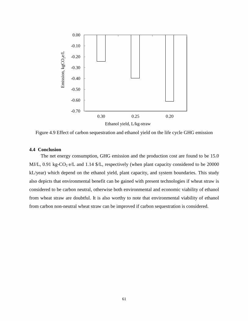
The net energy consumption, GHG emissions and production cost of ethanol were found to
be dependent on ethanol yield, feedstock cost, processing plant capacity and assumptions. This
study revealed that environmental benefit can be gained from biomasses, the economic viability
and biomass logistics of agri- and forest residues remain doubtful, unless a nominal subsidy (for
example FiT) is provided. The CLG process seems to be useful to reduce net energy
consumption and GHG emissions for both torrefied and non-torrefied miscanthus. Consequently,
Page 3
iii
miscanthus has emerged as a promising feedstock for ethanol industries (both enzymatic
hydrolysis and biosynthesis) even if it is grown on marginal land in Ontario, avoids any sort of
competition with food crops for higher quality land, avoids the food vs fuel debate, and improves
farm income and the rural economy. Eastern Ontario has emerged as the best option for
miscanthus based ethanol industry.
This study also revealed that syngas can be fermented with Clostridium Ljungdahlii into
ethanol by using the developed bioreactor. It is worthy to note that careful consideration has to
be placed on the land use changes, soil quality and their rebound effects if biomass, especially
agri-residues are to be put to use in the ethanol industry. The information generated in this study
has emerged to be novel and may help the stakeholders in their decision making processes, help
meeting the ethanol demand, and achieving GHG emissions target of Canada.
Page 4
iv
This thesis is dedicated to my loved Parents (Late Sahadeb Roy & Late Bimola Roy), who are
always remembered and in the center of all kind of inspiration in the life of the author.
Page 5
v
Acknowledgements
The author wishes to express his deepest sense of gratitude to his advisor Dr. Animesh
Dutta, School of Engineering, University of Guelph, Ontario, Canada for the institutional support
and scholastic supervision, constructive criticism and constant encouragement during the entire
period of this study.
He extend heartfelt gratitude to Dr. Bill Deen, Department of Plant Agricultural, Dr.
Brajesh Dubey and Dr. Shohel Mahmud, School of Engineering, University University of
Guelph, not only for serving in the Advisory Committee and extending their valuable time to
review this manuscript, but also for their thoughtful remarks, useful suggestions and constructive
criticism during this study. He also likes to thank Prof. Amar Mohanty and Dr. Fantahun M.
Defersha for their service in the qualifying examination committee and constructive suggestions.
The author is also thankful to Dr. Douglas M. Joy, Graduate Coordinator for his fruitful
suggestion during the qualifying examination. The author also likes to thank Dr. Sheng Chang
and Mr. Richard Chen for their support in preparing the membrane separator used in this study.
The author wishes to extend his appreciation to Mr. Michael Speagle for his ever-ready-to-
help in the laboratory activities and experimental setups. He also likes to thank Mrs. Carly
Fennell and Mrs. Joanne Ryks, Mr. Ryan Smith, and Mr. John Whiteside for extending their
helping hand, especially for the syngas fermentation study and computer related issues,
respectively. He would like to thank all the members of Dr. Dutta’s research team: Dr. Bimal
Acharya, Mr. Harpreet Kambo, Mr. Stefan Goupal, Mr. Jamie Minarat, Mr. MD Tushar, Dr.
Mathias Leon and Mr. Subhash Paul for their generous help and friendly companion during this
study. He is also indebted to Ontario Graduate Scholarship (OGS) Program for awarding the
prestigious scholarship during this study. The author also acknowledges for the Dean’s
scholarship from the University of Guelph.
The author feels proud to acknowledge his beloved wife Rita Roy who made a fruitful life
for the author during the entire period of this study and for her constant encouragement. He is
also thankful to his daughter Riya Roy for her love, which gives all kind of inspiration. The
author is also grateful to all of his family members and relatives for their moral support, enduring
patience and positive encouragement throughout his study in the University of Guelph, Ontario,
Canada. Finally, he wishes to express his sincere appreciation to those who have contributed
directly or indirectly for the successful completion of this study.
Page 6
vi
Table of Contents
Cover ................................................................................................................................................ i
Abstract ........................................................................................................................................... ii
Dedication ...................................................................................................................................... iv
Acknowledgements ........................................................................................................................ v
Table of Contents .......................................................................................................................... vi
List of Tables ............................................................................................................................... xii
List of Figures .............................................................................................................................. xiii
Chapter 1: Introduction ...................................................................................................................... 1
1.1. Rationale .......................................................................................................................................... 1
1.2. Objectives ......................................................................................................................................... 5
1.3. Scope and limitation of this research ............................................................................................... 6
1.4 Novelty of the research .................................................................................................................... 7
1.4.1 Bioreactor development............................................................................................................ 7
1.4.2 Chemical looping gasification (CLG) ...................................................................................... 7
1.4.3 Life cycle assessment ............................................................................................................... 8
1.5 Contribution of this research ............................................................................................................ 8
1.6 Publications from this research ...................................................................................................... 10
1.6.1 Publications in peer reviewed journals ................................................................................... 10
1.6.2 Submitted manuscripts ........................................................................................................... 10
1.6.3 Publications: Research presentations ..................................................................................... 10
Chapter 2: Literature Review ........................................................................................................... 11
2.1. Ethanol production via biochemical conversion process (enzymatic hydrolysis).......................... 11
2.1.1. Pretreatment ............................................................................................................................ 11
2.1.2. Fermentation ........................................................................................................................... 12
2.1.3. Distillation and purification .................................................................................................... 13
2.1.4. Waste management ................................................................................................................. 14
2.2. Life cycle assessment (LCA) of ethanol produced by biochemical conversion process ............... 16
2.2.1. LCA of ethanol produced from agri-residues ......................................................................... 16
2.2.2. L CA of ethanol from energy crops, woody biomass and forest residues .............................. 19
2.2.3. Land, water and other approaches in LCA of ethanol ............................................................ 22
Page 7
vii
2.3. Ethanol production via gasification process................................................................................... 24
2.3.1. Gasification ............................................................................................................................ 24
2.3.2. Gas cleanup ............................................................................................................................ 28
2.3.3. Syngas synthesis into ethanol ................................................................................................. 28
2.4 Life cycle cost analysis (LCCA) ....................................................................................................... 32
2.4.1 Life cycle costing of ethanol produced by biochemical process ............................................ 33
2.4.2 Life cycle costing of ethanol produced by thermochemical process ...................................... 37
Chapter 3: Life Cycle Assessment (LCA) Methodologies .............................................................. 41
3.1 LCA Methodologies ....................................................................................................................... 41
3.1.1 Goal definition and scoping.................................................................................................... 42
3.1.2 Life cycle inventory (LCI) analysis ........................................................................................ 45
3.1.3 Impact assessment .................................................................................................................. 46
3.1.4 Interpretation .......................................................................................................................... 46
3.2 Life cycle cost analysis (LCCA) .................................................................................................... 47
Chapter 4: Life Cycle Assessment of Ethanol produced from Wheat Straw ............................... 49
4.1 Introduction .................................................................................................................................... 49
4.2 Materials and methods ................................................................................................................... 49
4.2.1 System boundary .................................................................................................................... 49
4.2.2 Biochemical conversion process ............................................................................................ 50
4.2.3 Cost analysis ........................................................................................................................... 52
4.2.4 Data collection ........................................................................................................................ 52
4.3 Results and discussion ...................................................................................................................... 53
4.3.1 Energy consumption, CO2 emission and production cost ...................................................... 53
4.3.2 Sensitivity analysis ................................................................................................................. 56
4.4 Conclusion ..................................................................................................................................... 61
Chapter 5: Life cycle assessment of ethanol derived from sawdust .............................................. 62
5.1 Introduction .................................................................................................................................... 62
5.2 Methodology .................................................................................................................................. 62
5.2.1 System boundary and assumptions ......................................................................................... 62
5.2.2 Ethanol production ................................................................................................................. 64
5.2.3 Cost analysis ........................................................................................................................... 65
5.2.4 Data collection ........................................................................................................................ 65
Page 8
viii
5.3 Results and discussion.................................................................................................................... 66
5.3.1 Net energy consumption and CO2 emission ........................................................................... 66
5.3.2 Production cost ....................................................................................................................... 68
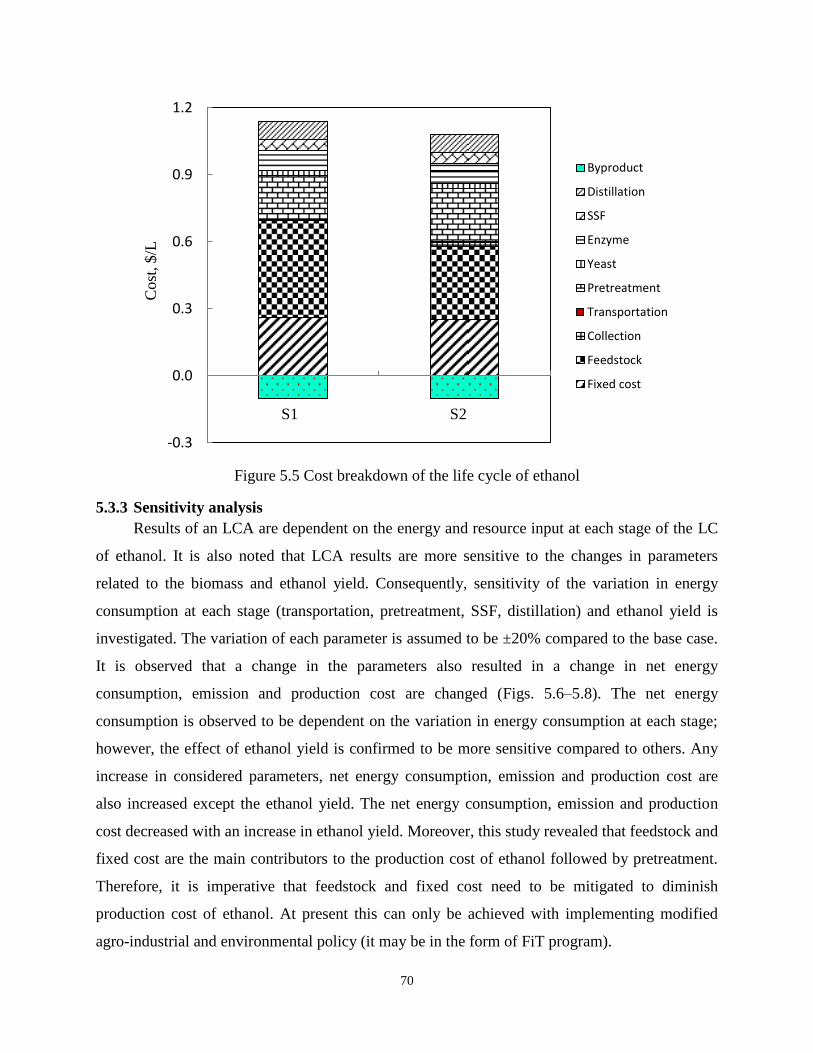
5.3.3 Sensitivity analysis ................................................................................................................. 70
5.4 Conclusion ..................................................................................................................................... 73
Chapter 6: Evaluation of the Life Cycle of Ethanol derived from Miscanthus in Ontario......... 74
6.1 Introduction .................................................................................................................................... 74
6.2 Methodology .................................................................................................................................. 75
6.2.1 Study area, system boundary and assumptions ...................................................................... 75
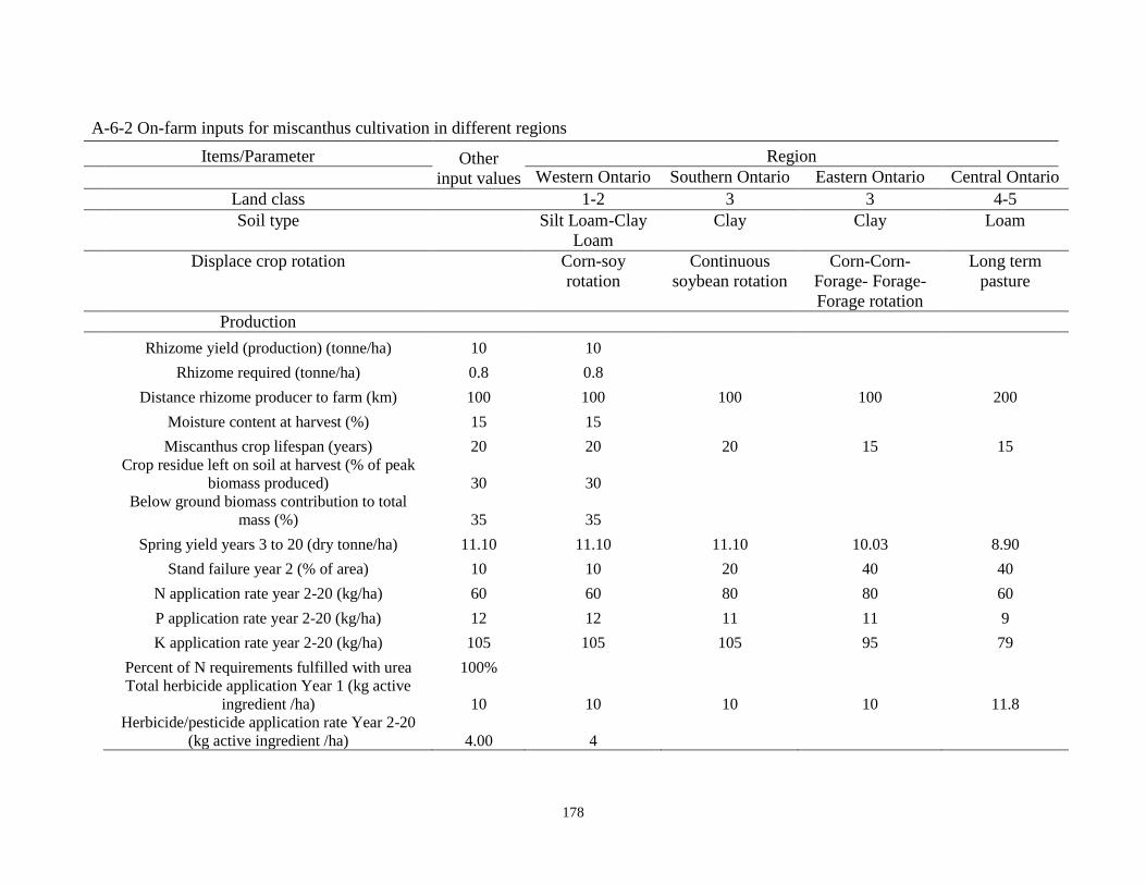
6.2.2 Miscanthus cultivation ........................................................................................................... 78
6.2.3 Transportation ........................................................................................................................ 80
6.2.4 Ethanol production ................................................................................................................. 80
6.2.5 Cost analysis ........................................................................................................................... 82
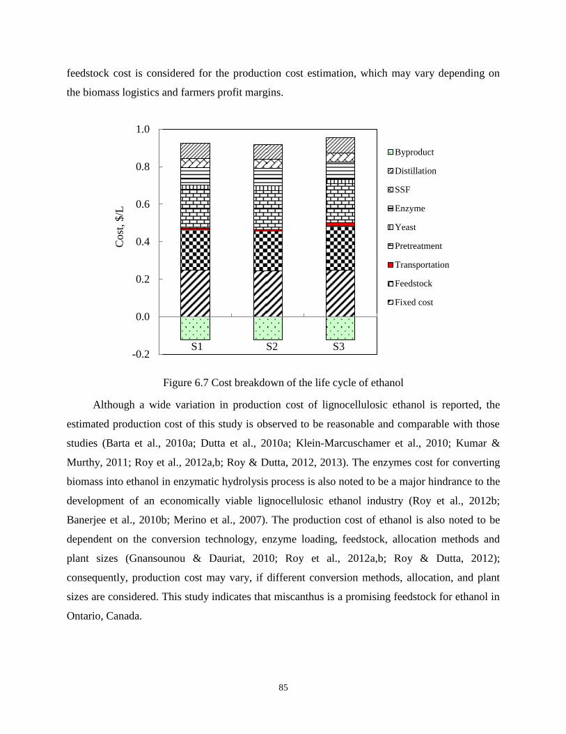
6.3 Results and discussion ...................................................................................................................... 82
6.3.1 Net energy consumption ............................................................................................................ 82
6.3.2 Greenhouse gas emission (CO2e) ........................................................................................... 83
6.3.3 Net production cost ................................................................................................................ 84
6.3.4 Sensitivity analysis ................................................................................................................. 86
6.4 Conclusion ..................................................................................................................................... 90
Chapter 7: Identification of suitable plant location for ethanol industry in Ontario, Canada ... 91
7.1 Introduction ............................................................................................................................... 91
7.2 Materials and methods ................................................................................................................... 91
7.2.1 Study area ............................................................................................................................... 91
7.2.2 System boundary .................................................................................................................... 91
7.2.3 Transportation, ethanol production and cost analysis ............................................................ 92
7.3 Results and discussion.................................................................................................................... 93
7.3.1 Net energy consumption ......................................................................................................... 93
7.3.2 Greenhouse gas emission (CO2 e) ........................................................................................... 94
7.3.3 Production cost ....................................................................................................................... 97
7.3.4 Sensitivity analysis ................................................................................................................. 98
7.4 Conclusion ................................................................................................................................... 102
Chapter 8: Development of a Continuous Stirred Tank Bioreactor for Syngas Fermentation 103
Page 9
ix
8.1 Introduction .................................................................................................................................. 103
8.2 Materials and Methods ................................................................................................................. 104
8.2.1 Reactor development ............................................................................................................ 104
8.2.2 Microorganism and media .................................................................................................... 106
8.2.3 Syngas fermentation ............................................................................................................. 106
8.2.4 Analytical method ................................................................................................................ 109
8.3 Results and discussion.................................................................................................................. 109
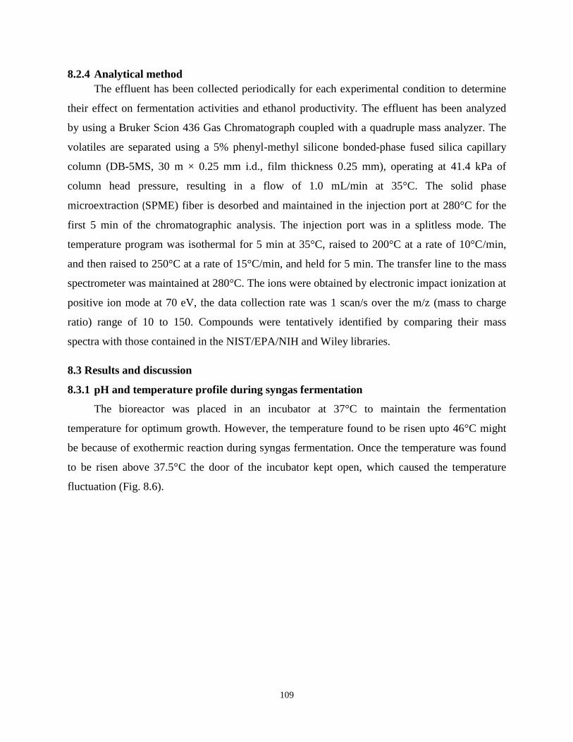
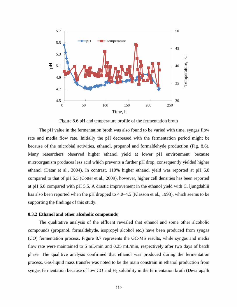
8.3.1 pH and temperature profile during syngas fermentation ...................................................... 109
8.3.2 Ethanol and other alcoholic compounds ............................................................................... 110
8.4 Conclusion ................................................................................................................................... 111
Chapter 9: Evaluation of the Life Cycle of Ethanol derived from Biosyngas Fermentation .... 112
9.1 Introduction .................................................................................................................................. 112
9.2 Materials and methods ................................................................................................................. 113
9.2.1 System boundary and assumptions ....................................................................................... 113
9.2.2 Pretreatment (torrefaction) ................................................................................................... 113
9.2.3 Ultimate analysis .................................................................................................................. 114
9.2.4 Gasification and syngas cleaning ......................................................................................... 114
9.2.5 Syngas fermentation ............................................................................................................. 115
9.2.6 Separation (distillation & purification) ................................................................................ 116
9.2.7 Waste management ............................................................................................................... 117
9.2.8 Cost analysis ......................................................................................................................... 117
9.2.9 Data collection ...................................................................................................................... 117
9.3 Results and discussion.................................................................................................................. 117
9.3.1 Net energy consumption ....................................................................................................... 117
9.3.2 GHG emission (CO2e) .......................................................................................................... 119
9.3.3 Production cost ..................................................................................................................... 120
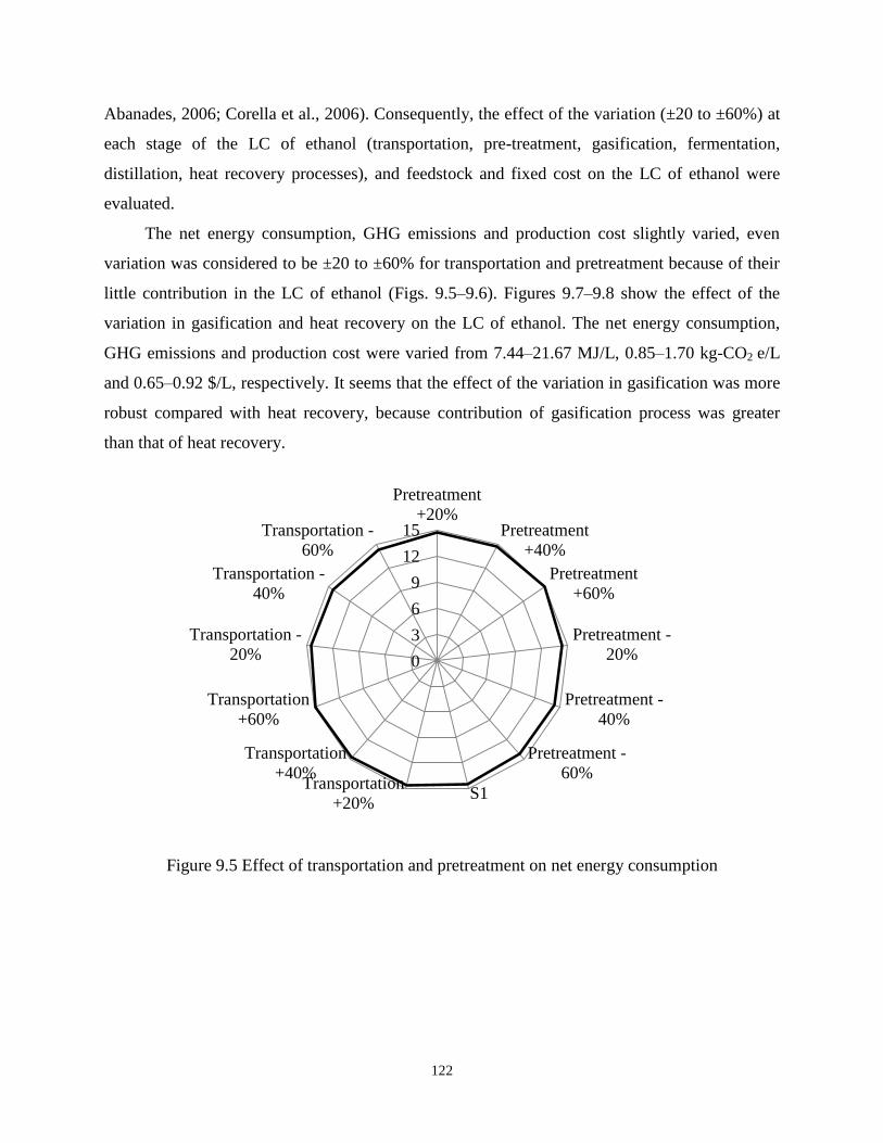
9.3.4 Sensitivity analysis ............................................................................................................... 121
9.4 Conclusion ...................................................................................................................................... 127
Chapter 10: Conclusions and Recommendations ......................................................................... 128
10.1 Conclusions .................................................................................................................................. 128
10.1.1 Evaluation of the LC of ethanol produced by enzymatic hydrolysis process ....................... 128
10.1.2 Evaluation of the LC of ethanol produced by gasification-biosynthesis process ................. 129
Page 10
x
10.1.3 Continuous stirred tank bioreactor ....................................................................................... 130
10.2 Recommendations ........................................................................................................................ 130
10.2.1 Life cycle assessment ........................................................................................................... 130
10.2.2 Improvement of bioreactor ................................................................................................... 130
Chapter 11: References ................................................................................................................... 132
Appendices ........................................................................................................................................ 170
A-2-1 The schematic diagram of chemical looping gasification (CLG) system ................................... 170
A-2-2 Brief summary of microorganisms identified and used for syngas fermentation ....................... 171
A-2-3 Syngas fermentation parameters and ethanol yield .................................................................... 175
A-6-1 Land classification in Ontario .................................................................................................... 177
A-6-2 On-farm inputs for miscanthus cultivation in different regions ................................................. 178
A-6-3 On-farm energy and other inputs for miscanthus cultivation ..................................................... 180
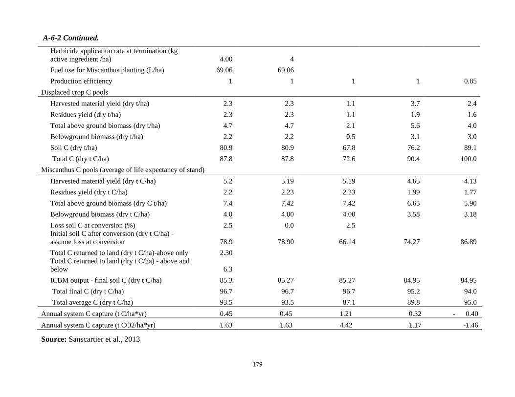
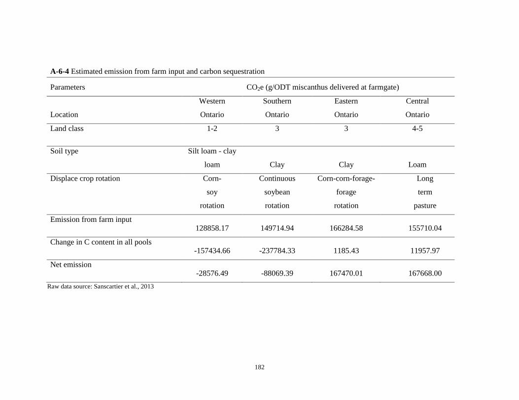
A-6-4 Estimated emission from farm input and carbon sequestration .................................................. 182
A-6-5 Calculation of energy consumption and material cost of enzyme production ............................ 183
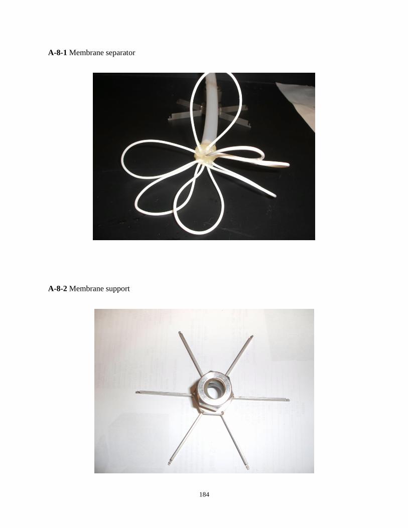
A-8-1 Membrane separator ................................................................................................................... 184
A-8-2 Membrane support ...................................................................................................................... 184
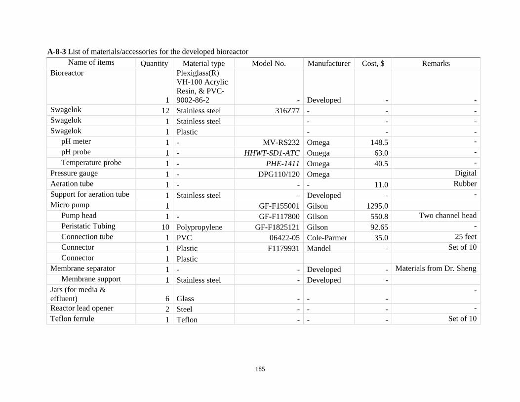
A-8-3 List of materials/accessories for the developed bioreactor ......................................................... 185
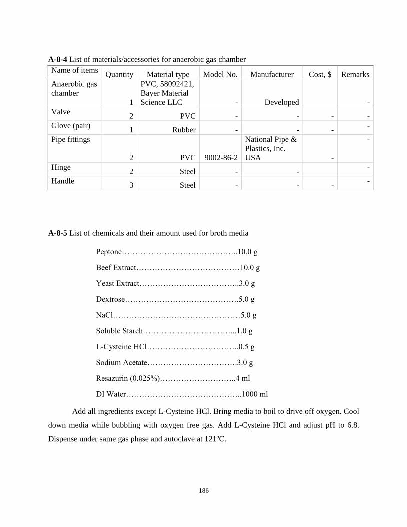
A-8-4 List of materials/accessories for anaerobic gas chamber ............................................................ 186
A-8-5 List of chemicals and their amount used for broth media .......................................................... 186
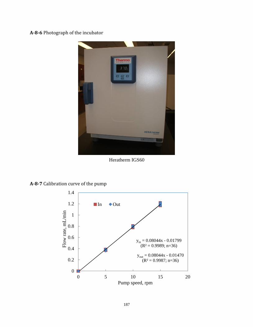
A-8-6 Photograph of the incubator ....................................................................................................... 187
A-8-7 Calibration curve of the pump .................................................................................................... 187
A-8-8 Photographs of overall experimental setup ................................................................................ 188
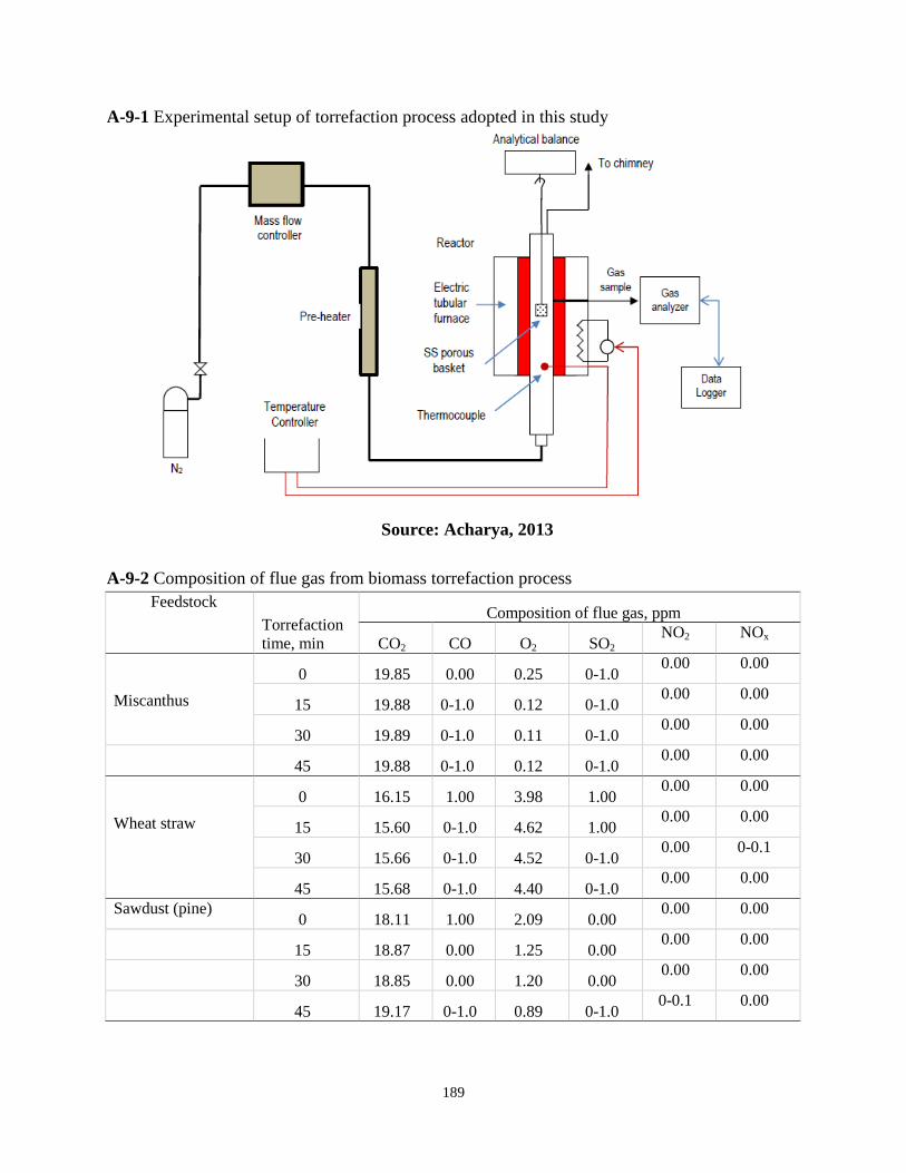
A-9-1 Experimental setup of torrefaction process adopted in this study .............................................. 189
A-9-2 Composition of flue gas from biomass torrefaction process ...................................................... 189
A-9-3 Energy consumption in the torrefaction of biomass (for 45 min) .............................................. 190
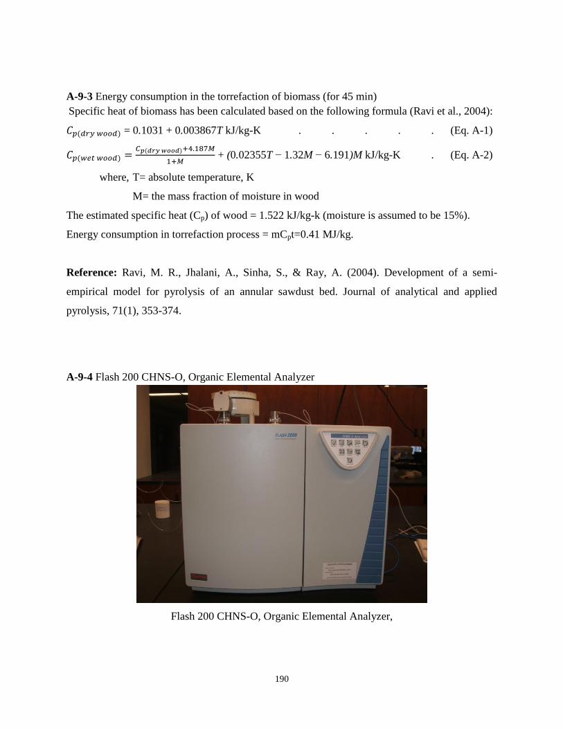
A-9-4 Flash 200 CHNS-O, Organic Elemental Analyzer ..................................................................... 190
A-9-5 Photograph of thermo gravimetric analyzer (TGA) ................................................................... 191
A-9-6 Photograph of Fourier transform infrared spectroscopy (FT-IR) ............................................... 191
A-9-7 TGA/FT-IR experimental parameters ........................................................................................ 192
A- 9-8 Comparison among various raw biomasses............................................................................... 192
Page 11
xi
A- 9-9 Comparison among various torrefied biomasses ....................................................................... 193
A- 9-10 Comparison among various raw biomasses degraded with CaO ............................................. 193
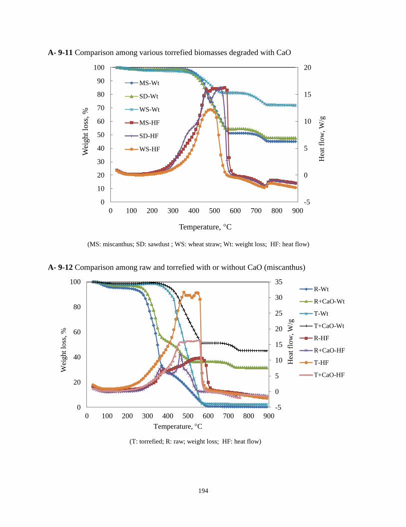
A- 9-11 Comparison among various torrefied biomasses degraded with CaO ..................................... 194
A- 9-12 Comparison among raw and torrefied with or without CaO (miscanthus) .............................. 194
A-9-13 Cold gas efficiency (CGE) calculation for steam gasification . ............................................... 195
A-9-14 Summary of ASPEN simulation parameters ............................................................................ 195
A-9-15 Summary of ASPEN simulation parameters and CLG block diagram..................................... 196
A-9-16 CLG simulation flowsheet ....................................................................................................... 197
A-9-17 Product gas compositions (simulated) and CGE ...................................................................... 198
Page 12
xii
List of Tables
Table 1.1 Projected biofuel production in major biofuel producing countries and in the world ....................... 2
Table 1.2 Lignocellulosic ethanol plants in Canada and their capacity ............................................................. 3
Table 2.1 Pretreatment processes of biomass .................................................................................................. 12
Table 2.2 Brief summary of energy consumption in distillation processes ..................................................... 15
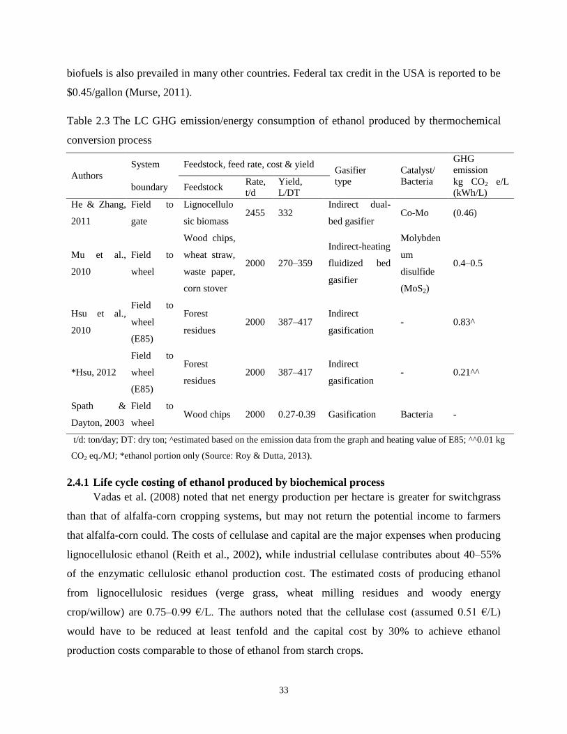
Table 2.3 The LC GHG emission/energy consumption of ethanol produced by thermochemical
conversion process ................................................................................................................................... 33
Table 2.4 Tax credits on ethanol in various provinces in Canada .................................................................... 34
Table 2.5 Summary of the reported cost of ethanol produced from different feedstocks (biochemical
conversion) ............................................................................................................................................... 38
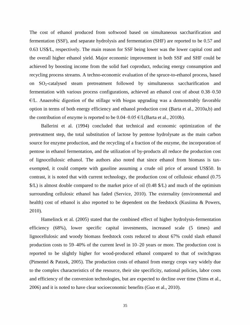
Table 2.6 Summary of the reported cost of ethanol from different feedstock and energy efficiency
(thermochemical conversion) ................................................................................................................... 40
Table 3.1 Mill residues production in Canada in 2004 (ODt: Oven dry tonnes) ............................................. 43
Table 3.2 Volatile matter, fixed carbon, and ash content in selected biomass (dry basis) ............................... 43
Table 3.3 Potential feedstocks and their major components ............................................................................ 44
Table 3.4 Chemical composition of different feedstock .................................................................................. 44
Table 4.1 Summary of parameters for which data are collected from the literature ........................................ 53
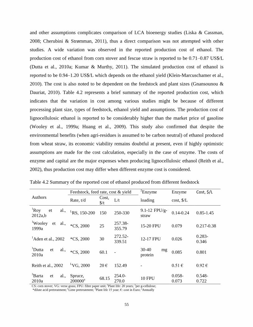
Table 4.2 Summary of the reported cost of ethanol produced from different feedstock ................................. 55
Table 4.3 Ethanol yield from wheat straw ....................................................................................................... 56
Table 5.1 Scenarios of this study. .................................................................................................................... 63
Table 5.2 Summary of parameters for which data are collected from literature .............................................. 66
Table 6.1 Land areas in Ontario, ha ................................................................................................................. 77
Table 6.2 Land classes, soil types and miscanthus yield ................................................................................. 77
Table 6.3 Scenarios of this study. .................................................................................................................... 78
Table 6.4 Summary of parameters for which data are collected from literature .............................................. 79
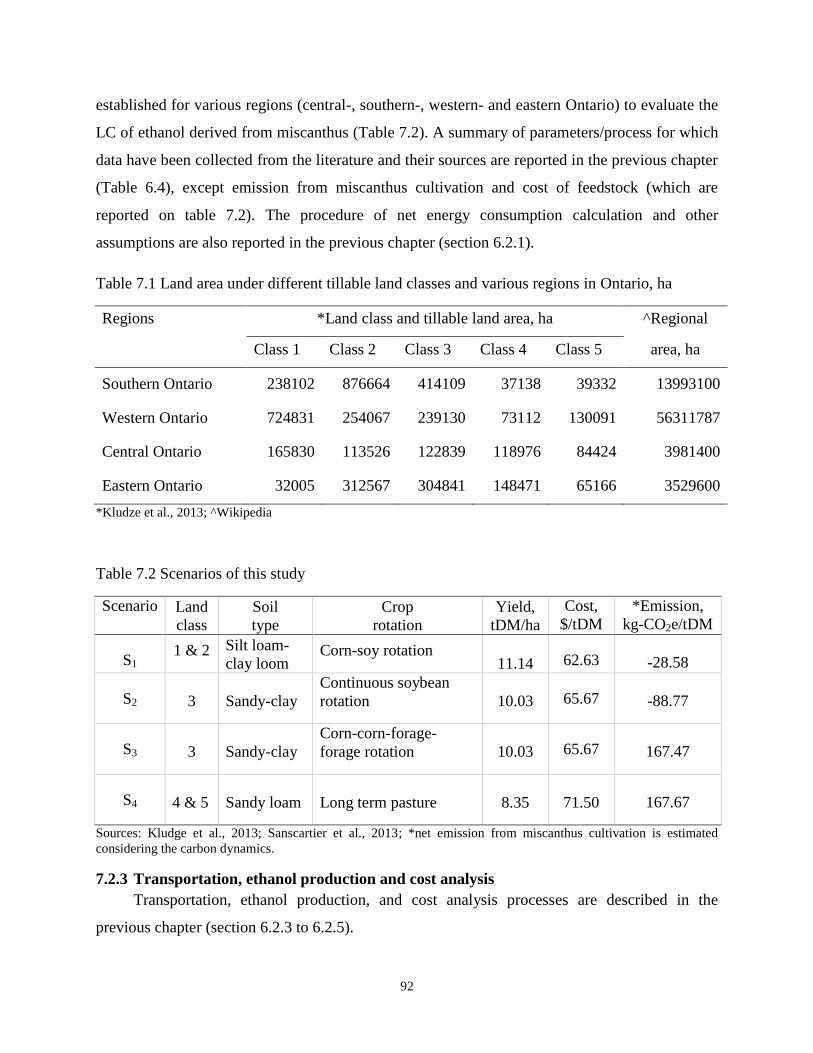
Table 7.1 Land area under different tillable land classes and various regions in Ontario, ha.......................... 92
Table 7.2 Scenarios of this study ..................................................................................................................... 92
Table 9.1 Components of different feedstock ................................................................................................ 114
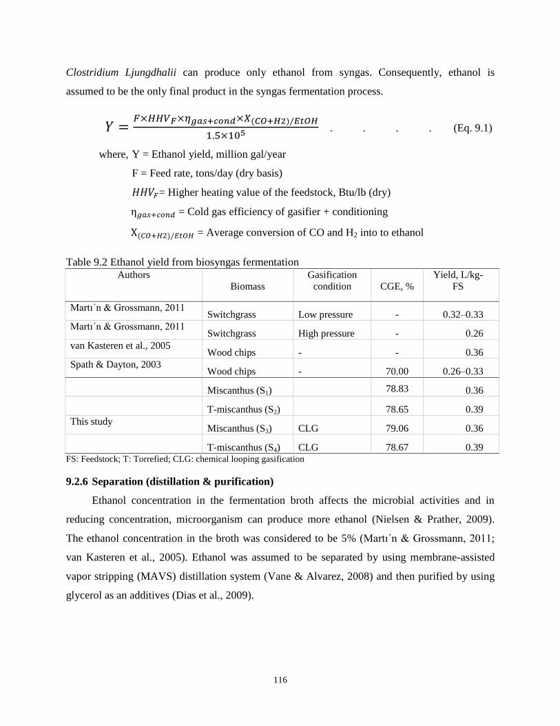
Table 9.2 Ethanol yield from biosyngas fermentation ................................................................................... 116
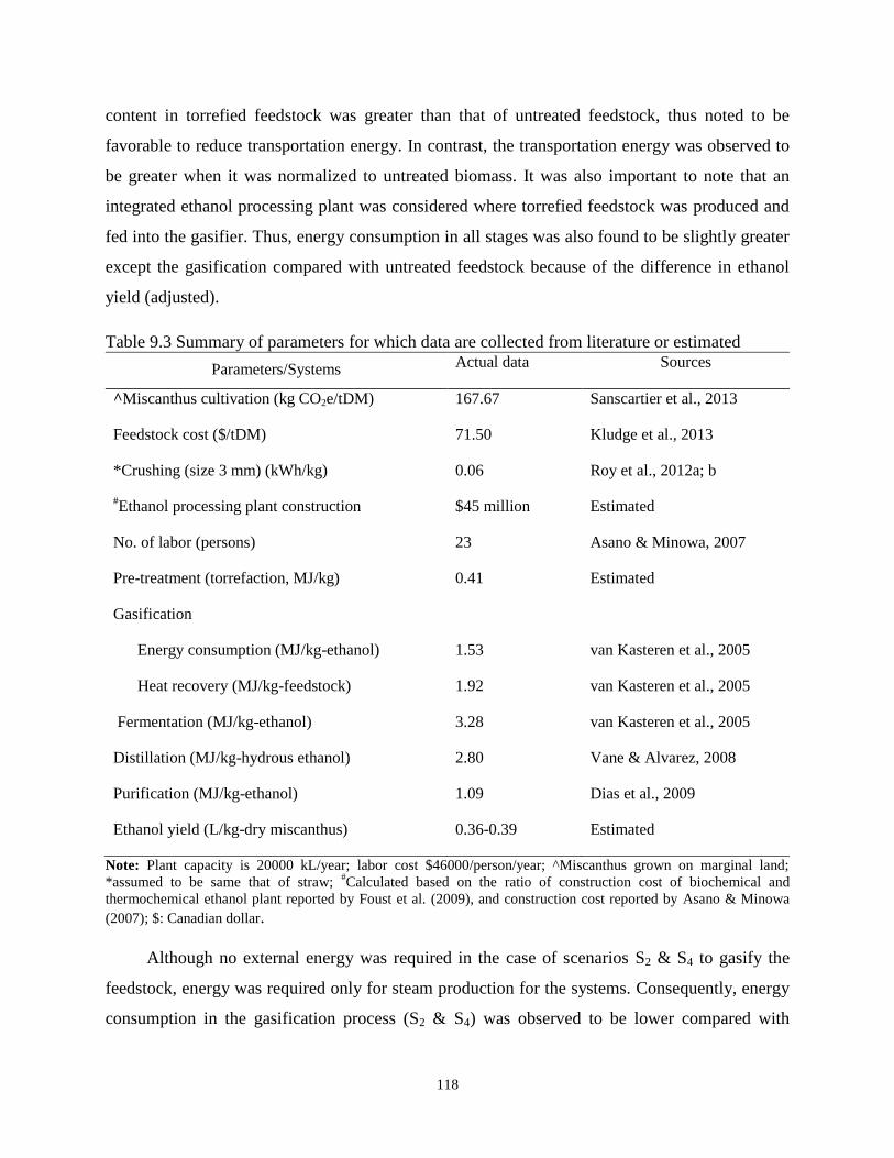
Table 9.3 Summary of parameters for which data are collected from literature or estimated ....................... 118
Page 13
xiii
List of Figures
Figure 1.1 Contribution of this study ................................................................................................................. 9
Figure 2.1Schematic diagram of ethanol production process from syngas...................................................... 27
Figure 3.1 Stages of an LCA (ISO, 2006) ........................................................................................................ 42
Figure 3.2 System boundary of this study ........................................................................................................ 45
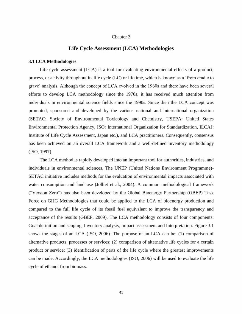
Figure 3.3 Structure of the LCIA method based on endpoint modeling (LIME2) ........................................... 47
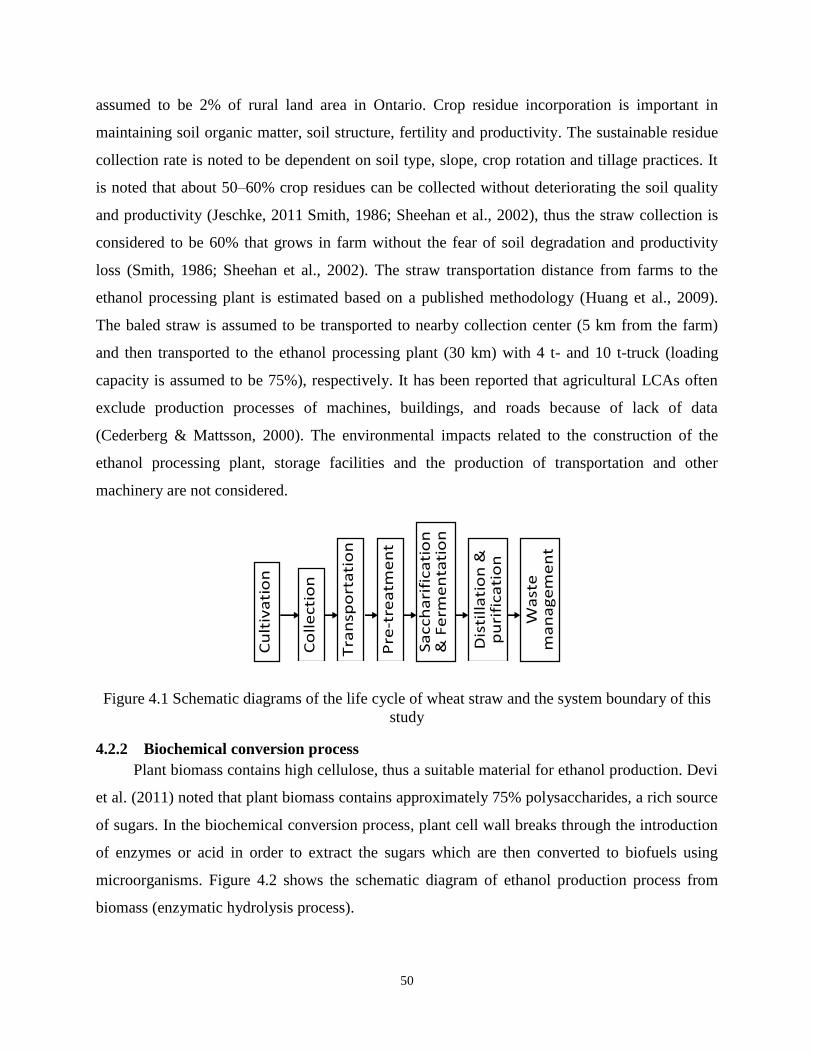
Figure 4.1 Schematic diagrams of the life cycle of wheat straw and the system boundary of this study ........ 50
Figure 4.2 Schematic diagram of ethanol production process from biomass .................................................. 51
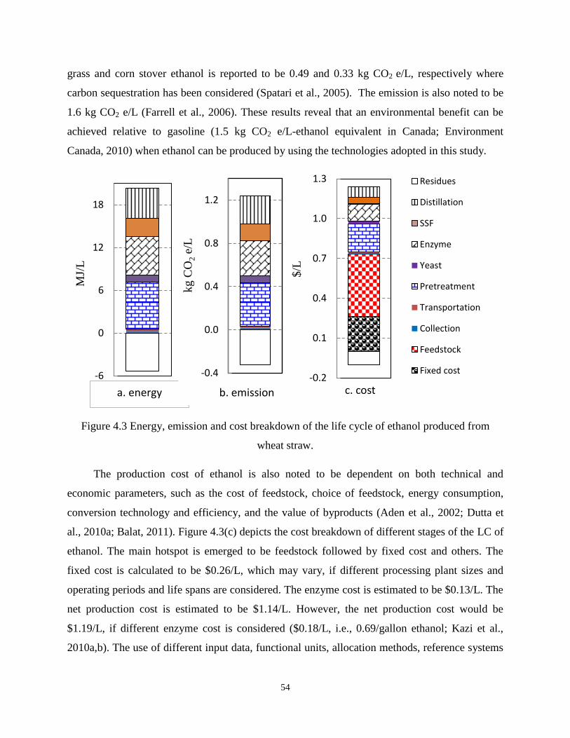
Figure 4.3 Energy, emission and cost breakdown of the life cycle of ethanol produced from wheat straw. ... 54
Figure 4.4 Effect of ethanol yield on net energy consumption, emission and production cost of ethanol ...... 57
Figure 4.5 Effect of feedstock cost on the production cost of ethanol ............................................................. 58
Figure 4.6 Effect of plant capacity on the production cost and emission of the life cycle of ethanol ............. 58
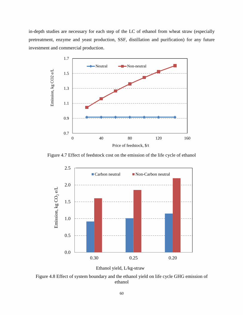
Figure 4.7 Effect of feedstock cost on the emission of the life cycle of ethanol ............................................. 60
Figure 4.8 Effect of system boundary and the ethanol yield on life cycle GHG emission of ethanol ............. 60
Figure 4.9 Effect of carbon sequestration and ethanol yield on the life cycle GHG emission ........................ 61
Figure 5.1 Schematic diagrams of the LC of sawdust and the system boundary of this study ........................ 64
Figure 5.2 Energy breakdown of the life cycle of ethanol ............................................................................... 67
Figure 5.3 Emission breakdown of the life cycle of ethanol ............................................................................ 68
Figure 5.4 Effect of carbon sequestration on the net emission of the life cycle of ethanol ............................. 69
Figure 5.5 Cost breakdown of the life cycle of ethanol ................................................................................... 70
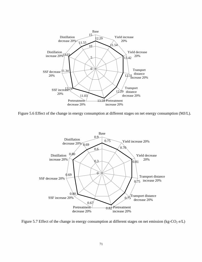
Figure 5.6 Effect of the change in energy consumption at different stages on net energy consumption. ........ 71
Figure 5.7 Effect of the change in energy consumption at different stages on net emission (kg-CO2 e/L) ..... 71
Figure 5.8 Effect of the change in energy consumption at different stages on net cost ($/L) .......................... 72
Figure 5.9 Effect of the changes in feedstock- and fixed cost on the production cost of ethanol .................... 72
Figure 6.1 Transportation fuel consumption and contribution of ethanol in Canada ...................................... 75
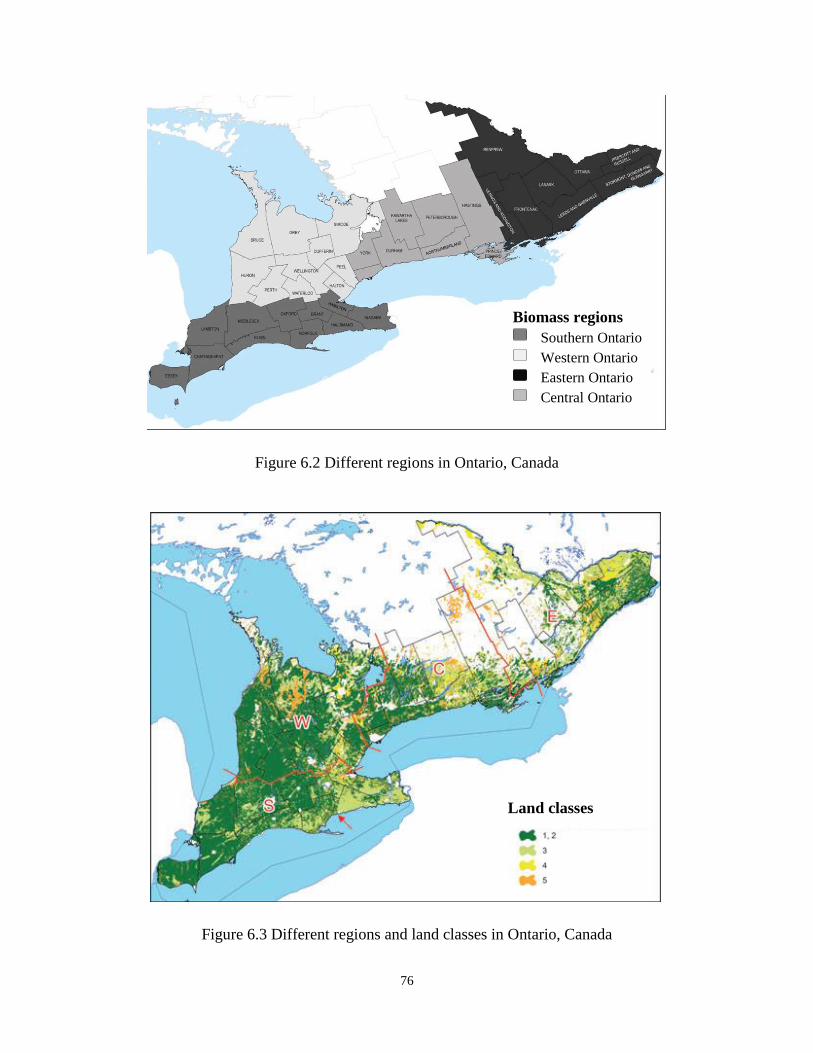
Figure 6.2 Different regions in Ontario, Canada ............................................................................................. 76
Figure 6.3 Different regions and land classes in Ontario, Canada ................................................................... 76
Figure 6.4 Schematic diagrams of the life cycle of sawdust and the system boundary of this study .............. 80
Figure 6.5 Energy breakdown of the life cycle of ethanol derived from miscanthus ...................................... 83
Figure 6.6 Emission breakdown of the life cycle of ethanol derived from miscanthus ................................... 84
Figure 6.7 Cost breakdown of the life cycle of ethanol ................................................................................... 85
Figure 6.8 Effect of the variation in transportation distance and pretreatment energy consumption on the
net energy consumption (MJ/L) ............................................................................................................... 87
Figure 6.9 Effect of the variation in transportation distance and pretreatment energy consumption on the
net emission and production cost ............................................................................................................. 88
Page 14
xiv
Figure 6.10 Effect of feedstock and fixed cost (S/L) ....................................................................................... 88
Figure 6.11 Effect of carbon dynamics on the net emission of the life cycle of ethanol ................................. 89
Figure 7.1 Feedstock transportation distance at different location in Ontario ................................................. 93
Figure 7.2 Energy breakdown of the life cycle of ethanol (Southern Ontario) ................................................ 94
Figure 7.3 Net energy consumption at different location in Ontario ............................................................... 95
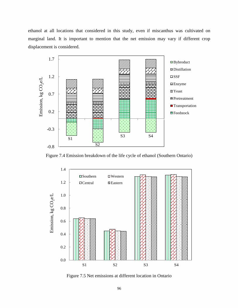
Figure 7.4 Emission breakdown of the life cycle of ethanol (Southern Ontario) ............................................ 96
Figure 7.5 Net emissions at different location in Ontario ................................................................................ 96
Figure 7.6 Cost breakdown of the life cycle of ethanol (Southern Ontario) .................................................... 97
Figure 7.7 Net production cost at different location in Ontario. ...................................................................... 98
Figure 7.8 Effect of ethanol plant capacity on production cost and emission ................................................. 99
Figure 7.9 Effect of ethanol plant capacity on production cost and emission ............................................... 100
Figure 7.10 Effect of the variation of different parameters on net energy consumption (MJ/L) ................... 101
Figure 7.11 Effect of the variation of different parameters on net emission ................................................. 101
Figure 8.1 Photograph of the developed reactor ............................................................................................ 104
Figure 8.2 Schematic diagram of the gas chamber (not to scale) .................................................................. 105
Figure 8.3 Photograph of the developed gas chamber ................................................................................... 105
Figure 8.4 Photograph of the experimental setup .......................................................................................... 108
Figure 8.5 Schematic diagram of the experimental setup of this study ......................................................... 108
Figure 8.6 pH and temperature profile of the fermentation broth .................................................................. 110
Figure 8.7 Mass spectra of the effluent .......................................................................................................... 111
Figure 9.1 Schematic diagram of the system boundary of this study. ........................................................... 113
Figure 9.2 Energy consumption at various stages of the LC of ethanol ........................................................ 119
Figure 9.3 Emission at different stages of the LC of ethanol ......................................................................... 120
Figure 9.4 Production cost at different stages of the LC of ethanol .............................................................. 121
Figure 9.5 Effect of transportation and pretreatment on net energy consumption ......................................... 122
Figure 9.6 Effect of transportation and pretreatment on emission and cost ................................................... 123
Figure 9.7 Effect of the variation of gasification and heat recovery on net energy consumption (MJ/L) ..... 123
Figure 9.8 Effect of the variation of gasification and heat recovery on emission and cost ........................... 124
Figure 9.9 Effect of the variation of fermentation and distillation on net energy consumption (MJ/L) ........ 125
Figure 9.10 Effect of variation of fermentation and distillation on emission and cost .................................. 125
Figure 9.11 Effect of variation of fixed and feedstock cost on production cost ($/L) ................................... 126
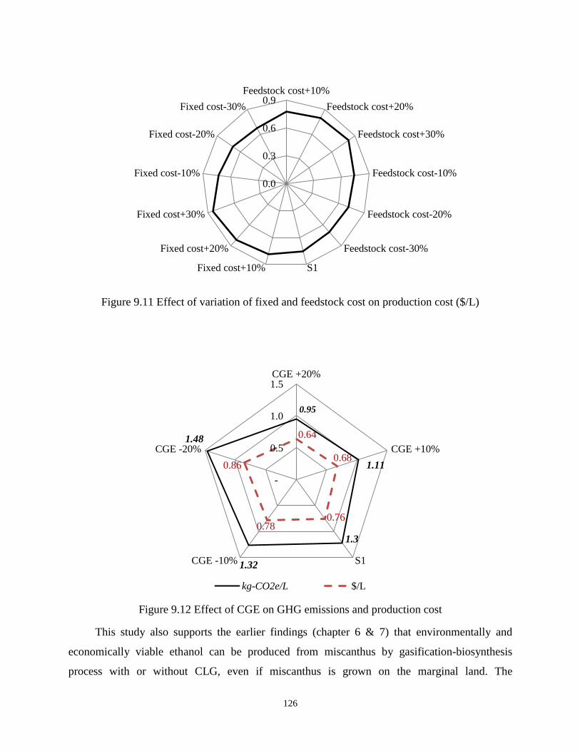
Figure 9.12 Effect of CGE on GHG emissions and production cost ............................................................. 126
Page 15
1
Chapter 1
Introduction
1.1. Rationale
The global energy demand was 424 EJ/year in 2000 and is increasing at the rate of 2.2%
per year (Lal, 2009) and the world’s total primary energy supply was reported to be 479 EJ in
2005 (GBEP, 2007). With existing technologies and consumption patterns, global energy
demand could double by 2050 due to the combination of population and economic growth
(UNEP, 2007). Greenhouse gas (GHG) emissions, which have increased remarkably due to
tremendous energy use liable for global warming, and perhaps the most serious problem that
humankind faces today. The growing concerns about climate change, rising costs of fossil fuels
and the geo-political uncertainty associated with possible interruption of current fossil fuel-based
energy supplies have motivated individuals, organizations and nations to seek clean and
renewable substitutes. Liquid biofuels (ethanol and biodiesel) are widely recognized alternatives
to fossil fuels. Table 1.1 represents the projected biofuel production in different regions.
Renewable energy not only reduces the reliance on foreign oil and improves energy security, but
also provides significant environmental benefits and enhances rural economies (Kim & Dale,
2003; Spatari et al., 2005; Farrell et al., 2006). In contrast, this rapid expansion affects virtually
every aspect of the field crop sectors and there remain an inevitable conflict between the
increasing diversion of crops or crop land for fuel instead of food (Liew et al., 2013). Biofuels
contain low sulphur, noted to be nontoxic, biodegradable and can reduce harmful GHG, carbon
monoxide, hydrocarbons and particulate matter (Mata et al., 2010).
The transportation sector in Canada accounts for about 25% of the nation's energy use and
the major part of this energy (99%) comes from fossil fuels (NRC, 2013). In 2009, Canada
committed to reduce total GHG emissions by 17% from 2005 levels by 2020. The Renewable
Energy Regulation (SOR/2010-189) was enacted (came-into-force from July 1, 2011) in Canada
which requires fuel producers and importers of gasoline to have renewable fuel content of at
least 5% distillates (by volume) that they produce and import yearly (Environment Canada,
2010), which generates a considerable demand on biofuels. The Government of Canada also
offers $0.10/L and $0.26/L operating incentive for ethanol and biodiesel, respectively, for up to
seven consecutive years (Biofuelnet, 2013). Consequently, the interest in biofuels is expanding.
The cellulosic ethanol processing plants in Canada and their production capacity is reported in
Page 16
2
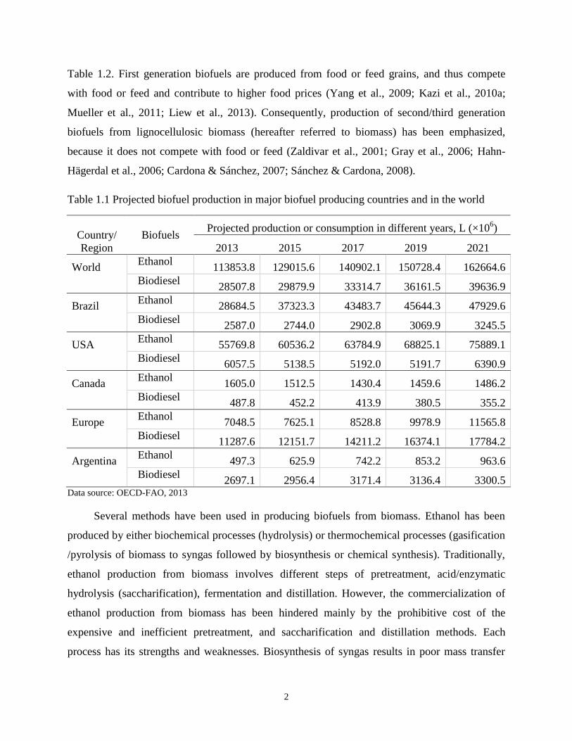
Table 1.2. First generation biofuels are produced from food or feed grains, and thus compete
with food or feed and contribute to higher food prices (Yang et al., 2009; Kazi et al., 2010a;
Mueller et al., 2011; Liew et al., 2013). Consequently, production of second/third generation
biofuels from lignocellulosic biomass (hereafter referred to biomass) has been emphasized,
because it does not compete with food or feed (Zaldivar et al., 2001; Gray et al., 2006; Hahn-
Hägerdal et al., 2006; Cardona & Sánchez, 2007; Sánchez & Cardona, 2008).
Table 1.1 Projected biofuel production in major biofuel producing countries and in the world
Country/
Region
Biofuels
Projected production or consumption in different years, L (×106)
2013 2015 2017 2019 2021
World Ethanol
113853.8 129015.6 140902.1 150728.4 162664.6
Biodiesel
28507.8 29879.9 33314.7 36161.5 39636.9
Brazil Ethanol
28684.5 37323.3 43483.7 45644.3 47929.6
Biodiesel
2587.0 2744.0 2902.8 3069.9 3245.5
USA Ethanol
55769.8 60536.2 63784.9 68825.1 75889.1
Biodiesel
6057.5 5138.5 5192.0 5191.7 6390.9
Canada Ethanol
1605.0 1512.5 1430.4 1459.6 1486.2
Biodiesel
487.8 452.2 413.9 380.5 355.2
Europe Ethanol
7048.5 7625.1 8528.8 9978.9 11565.8
Biodiesel
11287.6 12151.7 14211.2 16374.1 17784.2
Argentina Ethanol
497.3 625.9 742.2 853.2 963.6
Biodiesel
2697.1 2956.4 3171.4 3136.4 3300.5 Data source: OECD-FAO, 2013
Several methods have been used in producing biofuels from biomass. Ethanol has been
produced by either biochemical processes (hydrolysis) or thermochemical processes (gasification
/pyrolysis of biomass to syngas followed by biosynthesis or chemical synthesis). Traditionally,
ethanol production from biomass involves different steps of pretreatment, acid/enzymatic
hydrolysis (saccharification), fermentation and distillation. However, the commercialization of
ethanol production from biomass has been hindered mainly by the prohibitive cost of the
expensive and inefficient pretreatment, and saccharification and distillation methods. Each
process has its strengths and weaknesses. Biosynthesis of syngas results in poor mass transfer
Page 17
3
properties of gaseous substrates and low ethanol yield (Munasinghe & Khanal, 2010).
Conversely, higher ethanol yield was reported in this process (Clausen & Gaddy, 1993).
Biosynthesis is a two-stage process consisting of biomass gasification followed by microbial
fermentation of syngas into ethanol. This process may offer distinct advantages (utilization of
whole biomass including lignin, irrespective of biomass quality, elimination of complex
pretreatment steps and costly enzymes, higher specificity of biocatalysts, independence of the
H2/CO ratio, aseptic operation of syngas fermentation, bioreactor operation at ambient
conditions, no issue with inorganic catalyst poisoning due to trace sulphur containing gas) over
both hydrolysis-fermentation and gasification-catalytic synthesis (high pressure, temperature,
expensive metallic catalyst and complex gas cleaning). Traditional fermentations rely on
carbohydrates as the carbon and energy sources for the microbial growth; however, syngas
fermentation utilizes microorganisms (especially, the Clostridium family) capable of
metabolizing syngas into ethanol and other valuable chemicals in an inexpensive liquid substrate.
However, poor mass transfer between gaseous and liquid substrates is one of the most significant
challenges for this process.
Table 1.2 Lignocellulosic ethanol plants in Canada and their capacity
Company Location Feedstock
Capacity, 106
L/y Remarks
Enerkem Inc.
Westbury,
QC
Wood waste from used
utility poles, RDF 5 Existing
Iogen Corp. Ottawa, ON
Wheat Straw, Oat Straw,
Barley Straw, Bagasse 2 Existing
Enerkem/GreenField -
Varennes cellulosic
Ethanol LP
Varennes,
QC
RDF, C&D debris
38
Proposed
Mascoma Corp.
Drayton Valley
Drayton
Valley, AB
Hardwood
72
Proposed
Nipawin Biomass
Ethanol New
Generation Co-
operative Ltd.
Nipawin,
SK
Wood waste, Straw
100
Proposed
Woodland Biofuel Inc. Sarnia, ON Wood waste 0.5 Proposed
Source: EPM, 2014
Page 18
4
Although the thermochemical process produces ethanol in large quantities, it requires
expensive catalysts and high operating pressure (Subramani and Gangwal, 2008). Many
researchers have studied ethanol production processes from syngas either by biosynthesis or
catalytic synthesis process (Ruth, 2005; Martchamadol, 2007; Clausen & Gaddy, 2008;
Munasinghe & Khanal, 2010) except for few examples (Foust et al., 2009; Mu et al., 2010).
Bioenergy systems have also been modeled with Aspen Plus and evaluated to estimate
production cost and environmental impacts of bioenergy. GHG emissions and production cost of
biofuels were reported to be dependent on both technical and economic parameters, such as the
cost and choice of feedstock, conversion technologies and value of coproducts/byproducts
(Wyman, 1994; Ballerini et al., 1994; Wooley et al., 1999a; Aden et al., 2002; Mabee et al.,
2006; Aden, 2008; Dutta et al., 2010a; Balat, 2011). Thus, a wide variation was reported in the
case of GHG emissions and production cost. The cost of cellulase was the major expense when
producing lignocellulosic ethanol with conventional technology (Singh & Kumar, 2010) and
contributed about 40–55% of the enzymatic ethanol production cost. Distillation, enzyme
production and pretreatment were reported to be the main contributor to energy consumption and
GHG emissions in the LC of ethanol produced by conventional technology (Roy et al., 2012a,b;
Orikasa et al., 2009). The cost effective and innovative fermentation strategies integrated in the
technology chain of gasification and gas cleaning combined with syngas fermentation, and
catalytic synthesis could significantly improve the overall economics of ethanol from biomass.
Life cycle assessment (LCA) is a tool for evaluating environmental effects of a product,
process, or activity throughout its LC. The key objective of an LCA study is to provide as
complete a portrait as possible of energy consumption, environmental impacts, economic
viability and their rebound effects, hence enable effective planning for a sustainable society. This
study evaluated the LC of ethanol to estimate net energy consumption and GHG emissions to
identify the hotspots, improve the production process, and determine if environmentally friendly
ethanol can be produced from biomass. It is also known that environmental information
generated through an LCA, while useful, does not always provide a sufficient basis for making a
sound decision on an investment. The cost analysis along with the estimation of GHG emissions
broadens the process of making sound decisions. Therefore, the production cost of ethanol has
also been estimated with both fixed costs (straight line depreciation on installation, labor,
maintenance and interest on investment) and variable costs (feedstock, yeast/bacteria, utilities
Page 19
5
and waste management). The Aspen Plus process modeling has also been used for steady-state
simulation (for syngas composition and syngas production to calculate the cold gas efficiency).
Sensitivity analyses were also conducted to determine the acceptability, profitability and risk on
investment if any. Finally, the results were interpreted to communicate to the stakeholder,
environmental activist and policy makers, which may help investor and policy maker’s decision
and draw more investment in this sector.
1.2. Objectives
The goal of this research was to investigate the technical feasibility of ethanol derived from
biomass (crop/forest residues and energy crops) by hybrid thermochemical and
biochemical/chemical processing, considering innovative technologies [enzymatic hydrolysis:
pretreatment (CaCCO: calcium capturing by carbonation), vacuum extractive fermentation and
distillation; biosynthesis: with/without chemical looping gasification (CLG) of torrefied and non-
torrefied biomass]. At first, the conventional ethanol production processes were evaluated to
have the baseline information and then Aspen Plus simulation software has been used to gather
required data (especially for the gasification processes). Finally, the LC of ethanol produced by
the above mentioned innovative technologies have been evaluated by using the LCA
methodologies (centering on net energy consumption, GHG emissions and production cost) to
determine the environmentally preferable and economically viable energy pathway for Ontario,
Canada. This study developed/identified environmentally preferable and economically viable
innovative technology (either biochemical or thermochemical) for lignocellulosic ethanol, which
is renewable and clean, thus help in reducing GHG emissions from the present energy sector in
Canada, may enable to compete economically and technologically in the world ethanol markets,
and contribute to improve rural economy in Ontario, Canada.
The specific objectives of this study were:
i. Evaluate the LC of ethanol produced by conventional /traditional technology (enzymatic
hydrolysis).
ii. Develop a bioreactor for syngas fermentation into ethanol.
iii. Evaluate the LC of ethanol produced from syngas (biosynthesis). Both torrefied and
non-torrefied biomass were used for a novel CLG and steam gasification (without CLG)
processes.
iv. Determine the LC cost of ethanol.
Page 20
6
1.3. Scope and limitation of this research
This research consists of four individual objectives, the scope of those are explained
bellow.
i. Three types of feedstocks (wheat straw, sawdust and miscanthus) have been selected for
enzymatic hydrolysis process. The LC of ethanol produced from these feedstocks by
enzymatic hydrolysis process was evaluated based on the estimated and literature data.
Ontario specific data were collected from the literature for miscanthus cultivation. All
those data were neither site nor country specific nor from the same plant size. The plant
capacity was considered to be 20000 kL/yr. The yearly operation period and life span of
the processing plant was assumed to be 350 days and 20 years, respectively (Dutta et al.,
2011; Huang et al., 2009; Wu et al., 2006). Some optimistic literature data has also been
used in this study, especially the enzyme production.
ii. Mass transfer between liquid and gaseous substrates hinders the syngas fermentation
into ethanol. The bioreactor has been developed as a part of this study to improve the
mass transfer by incorporating an innovative gas supply system. In addition to this, a
membrane separation system has also been added to the reactor to extract the effluent
excluding the microorganism. The reactor has been tested with only CO instead of
syngas (60%CO; 35%H2 and 5%CO2) to prove the concept.
iii. The torrefied and non-torrefied biomass have been considered for gasification (with or
without CLG) processes. Thermal degradation experiments have been conducted with
TGA to determine the effectiveness of CLG. Aspen Plus simulation at equilibrium
condition has been used to generate data for syngas composition and volume to
calculate the cold gas efficiency, thus the ethanol yield. The estimated and literature
data have been used to evaluate the LC of ethanol produced by gasification-biosynthesis
process considering the plant capacity of 20000 kL/yr.
iv. The production cost has been determined based on both the fixed and variable costs.
The life span of an ethanol plant and an operation period was assumed to be 20 years
and 350 days per year, respectively (Dutta et al., 2011; Huang et al., 2009; Wu et al.,
2006). Both the estimated and literature data have been used to determine the
production cost.
Page 21
7
1.4 Novelty of the research
This research consists of both analytical and theoretical analysis (LCA: policy analysis)
which are thought to be a novel approach.
1.4.1 Bioreactor development
A novel continuous stir-tank bioreactor (consists of innovative gas supply and effluent
extraction processes) has been developed to produce ethanol from syngas by using
microorganism. Innovative systems for syngas supply and ethanol extraction have also been
developed to improve gas-liquid mass transfer and reuse of microorganism. The research also
attempted to produce ethanol from syngas by using the developed bioreactor.
1.4.2 Chemical looping gasification (CLG)
Biomass characteristics have been determined at the laboratory, and those properties were
applied for further studies. A macro-reactor (QWM: Quartz wool matrix) was used for the
torrefaction process. The thermal degradation properties were also determined. The weight loss
and heat flow during the degradation process were monitored in a micro-reactor (TGA-FTIR).
The CLG concept consists of two fluidized bed reactors (operate parallely), which were
functioning as calciner and gasifier. In the calciner, limestone was calcined. Lime was then
circulated to the reactor (gasifier), where the lime sorbent was carbonated in parallel with the
gasification reactions, tying up most of the CO2 as CaCO3. The CaCO3 was then recirculated to
the calciner, acting as a regenerator. This looping concept has definite economic promise, and
was particularly attractive in the gasification processes, where it has added benefits-shifting the
equilibrium to yield more hydrogen, releasing heat in the reactor (where the main reactions were
endothermic), reducing loss of activity, and decreasing tar formation, at the same time capturing
CO2 produced during gasification.
Aspen Plus (V7.3) simulation software has been used to determine the syngas productivity
and gas composition at equilibrium condition for treated (torrefied) and untreated feedstock with
(CLG: chemical looping gasification) or without CO2 capture. The novelty of the CLG process
lies in the generation of relatively pure H2 from biomass on a continuous basis, while CO2
produces as a byproduct using steam as the gasifying agent. Another unique feature of the
process is internal regeneration of the sorbent, fouled in the gasifier. The technology served the
twin purpose of regenerating the sorbent, and generation of relatively clean syngas which is a
novel approach. Utilization of torrefied biomass in ethanol production process is also known to
Page 22
8
be a novel idea and is a novelty of this research. Thus, it will open up a new area of research on
H2-enriched gas production from biomass with in-process CO2 capture. The specific new
information generated by this study are as follows:
Torrefied and non-torrefied feedstock has been used in the CLG process.
Torrefied feedstock produced relatively better quality syngas.
The use of torrefied feedstock in ethanol production process.
1.4.3 Life cycle assessment
The research evaluated the life cycle (LC) of ethanol produced from various feedstocks
(wheat straw, sawdust and miscanthus), identified the feedstock and locations for ethanol
industry in Ontario, Canada; especially, from energy crop (miscanthus) by using hybrid
enzymatic hydrolysis and biosynthesis (syngas fermentation) processes. Both the
technoeconomic and environmental evaluation were carried out by adopting the life cycle
assessment (LCA) methodologies. The LCA methodologies also identify hotspots, and help to
improve the production process. The main hotspots identified are either pretreatment, feedstock
or gasification in the case of GHG emissions, depending on the type of feedstock, and scenario
or the conversion technology. The LCA study on the ethanol production process which
incorporated the torrefaction and the chemical looping gasification (CLG) is also a novel
approach. The novel information generated in this study would be useful to researchers, investors
and policy makers which might help Ontario compete economically and technologically in the
world ethanol markets, and contribute to improve rural economies in Canada. The specific new
and novel information generated by this study are as follows:
This study generated new information on lignocellulosic ethanol in the context of
Ontario.
Identified the potential location for miscanthus based ethanol industry in Ontario.
Life cycle of ethanol from torrefied and non-torrefied feedstocks with or without CLG
has also been evaluated, which is a novel work of this kind.
1.5 Contribution of this research
The following diagram briefly represents the plan, background and contribution of this
study (Fig. 1.1).
Page 23
9
Figure 1.1 Contribution of this study
Research on
torrefied biomass
thermal degradation
with or without CaO
is limited.
Syngas fermentation
with microorganism
in an innovative
reactor is scarce.
Life cycle of ethanol
from lignocellulosic
biomass, wheat straw,
sawdust and
miscanthus which
received limited
attention.
LCA of syngas
fermentation
(biosynthesis) is scarce
Ste
am g
asif
icat
ion w
ith o
r
wit
hout
CL
G o
f tr
eate
d o
r
untr
eate
d
bio
mas
s is
sca
rce
Stu
die
s on i
nnovat
ive
gas
su
pply
and e
fflu
ent
extr
acti
on
is l
imit
ted
LCA of ethanol derived from lignocellulosic biomass
Pla
nned
B
ackgro
und
Experiments Simulation LCA & LCCA Bioreactor
Contr
ibuti
on
Biomass
characterization
Torrefaction of
biomass in QWM
fluidized bed reactor
Thermal degradation
with or without CaO
in a micro-gasifier
(TGA)
Syngas fermentation
with microorganism
for ethanol
Syngas
com
posi
tion a
nd s
yngas
pro
duct
ivit
y a
re s
imula
ted b
y A
SP
EN
Plu
s si
mula
tion s
oft
war
e
A n
ovel
bio
reac
tor
has
bee
n d
edel
oped
whic
h c
onsi
sts
of
innovat
ive
gas
supply
and e
fflu
ent
extr
acti
on m
ethods
LCA and LCCA of
ethanol produced from
wheat straw, sawdust,
miscanthus by
enzymatic hydrolysis
process
LCA and LCCA of
ethanol derived from
syngas (gasification-
biosynthesis path) from
treated or untreated
biomass with or without
CLG.
(QWM: quartz wool matrix, TGA: Thermo gravimetric anatysis, LCCA: life cycle cost analysis)
Page 24
10
1.6 Publications from this research
1.6.1 Publications in peer reviewed journals
Life cycle assessment of ethanol derived from sawdust. Poritosh Roy & Animesh Dutta,
2013. Bioresource Technology, 150(December), 407–411.
A review of life cycle of ethanol produced from bio syngas. Poritosh Roy & Animesh
Dutta, 2013. Bioethanol, 1(1), 9–19.
Life cycle assessment of ethanol produced from wheat straw. Poritosh Roy & Animesh
Dutta, 2012. Journal of Biobased Materials and Bioenergy, 6(3), 276–282.
1.6.2 Submitted manuscripts
Evaluation of the life cycle of ethanol derived from miscanthus in Ontario, Canada.
Poritosh Roy, Animesh Dutta & Bill Deen, 2014. (Biomass and Bioenergy).
Review on syngas fermentation processes for bioethanol. Bimal Acharya, Poritosh Roy &
Animesh Dutta, 2014. (Biofuels).
1.6.3 Publications: Research presentations
The potential location for lignocellulosic ethanol processing plant in Ontario. Poritosh
Roy, Animesh Dutta & Bill Deen, 2014. 13th
International Symposium on Bioplastics,
Biocomposites & Biorefining: Moving towards a Sustainable Bioeconomy, Guelph,
Ontario, Canada, May 19–24.
Miscanthus: A promising feedstock for ethanol in Ontario. Poritosh Roy, Animesh
Dutta & Bill Deen, 2013. Bioeconomy Research Highlights Poster Showcase, Guelph,
Ontario, Canada, November 27.
Evaluation of the life cycle of ethanol produced from agri-residues (wheat straw).
Poritosh Roy & Animesh Dutta, 2012. Growing the Margins/Canadian Farm & Food
Biogas Conferences, London, Canada, March 5–7.
Life cycle assessment of bioethanol produced from biomass. Poritosh Roy & Animesh
Dutta, 2011. Bioeconomy Research Highlights Poster Showcase, Guelph, Ontario,
Canada, December 7.
Page 25
11
Chapter 2
Literature Review
2.1. Ethanol production via biochemical conversion process (enzymatic hydrolysis)
2.1.1. Pretreatment
Pretreatment (either physical or chemical or both) is a prerequisite for biological
conversion of biomasses (Lynd et al., 2008; Yang & Wyman, 2008) to make them more
amenable to cellulose hydrolysis. Table 2.1 summarizes some pretreatment processes of biomass.
Physical pretreatment refers to the size reduction of feedstock to increase enzyme-accessible
surface areas (Zhu et al., 2009b) and chemical pretreatments remove or modify key chemical
components that interfere with biomass cellulose saccharification, mainly hemicelluloses and
lignin (Zhu et al., 2009a; Zhu & Pan, 2010). The potential pretreatment methods are: acid
hydrolysis (concentrated or diluted), liquid hot water extraction, steam explosion, dilute acid-
steam explosion, ammonia fiber explosion, lime pretreatment, etc. (Holtzapple et al., 1991;
Mosier, et al., 2005a,b; Wyman et al., 2005; Yang & Wyman, 2008; Huang et al., 2009; Banerjee
et al., 2010a; Manzanares et al., 2012). The acid pretreatments are reported to be toxic,
hazardous, and corrosive, and require expensive reactors resistant to corrosion and also causes
difficulties in waste management streams (Yang & Wyman, 2008).
High energy requirement and inhibitors generation are reported to be major drawback of
steam explosion method (Hendriks & Zeeman, 2009; Banerjee et al., 2010a). The cost of
ammonia, its handling, and recovery, and high energy consumption in recompression are the
main bottlenecks in the process (Banerjee et al., 2010a). On the other hand, the alkaline
pretreatment is reported to be more suitable and effective for herbaceous crops and agricultural
residues (Bjerre et al., 1996; Chang et al., 2001; Rabelo et al., 2009). The hot water pretreatment
avoids the formation of inhibitors and catalyze hydrolysis of cellulosic materials (Mosier et al.,
2005a; Yu et al., 2010). It is also reported that cost of lime is relatively low and safer reagent
compared with other alkalis and ammonia (Kaar & Holtzapple, 2000; Saha & Cotta, 2008). The
CaCCO (calcium capturing by carbonation) process has also been developed to facilitate the
pretreatment of biomass (Park et al., 2010; Shiroma et al., 2011). The author also noted that this
pretreatment can also be applied at room temperature (7 days and 10% lime) to facilitate the
conversion process. Pretreatment process contributes about 18–20% of the total cost of
Page 26
12
biological production of cellulosic ethanol, which is greater than any other single step of the LC
of ethanol (Aden et al., 2002; Yang & Wyman, 2008; Wooley et al., 1999b). Although the
pretreament to biomasses may vary depending on their characteristics (for example sawdust from
softwood vs hardwood), the hotwater pretreatment (with 10% lime) has been adopted for this
study (Park et al., 2010; Shiroma et al., 2011).
Table 2.1 Pretreatment processes of biomass
Methods Processes Remarks
Physical
Milling: ball, hammer, two-roll, colloid, vibro etc. High energy demand
Irradiation: microwave, electron-beam, gamma ray Cannot remove lignin
Others: torrefaction, extrusion, pyrolysis, high pressure
steam, hotwater etc.,
No chemicals are used
Physico-
chemical
Explosion: steam, ammonia fiber (AFEX), CO2, SO2
Alkali: NaOH, NH4, (NH4)2S, Ca(OH)2, RT-CaCCO,
ammonia recycled percolation (ARP), liquid ammonia
Low cost
Gas: NO2, ClO2, SO2
Acid: H2SO4, HCl, H3PO4 Complex downstream
Oxidizing: Hydrogen peroxide, wet oxidation, ozone
Solvent extraction: Ethanol-water, benzene-water,
ethylene glycol, butanol-water, swelling agents
SPORL: Acid with sulfite or bisulfite
Biological Fungi, actinomycetes Low energy requirement,
low treatment rate
Source: Taherzadeh & Karimi, 2008; Zhu et al., 2009a; Shiroma et al., 2011; Wilkins, 2011; Yoon et al., 1995.
2.1.2. Fermentation
Fermentation is the chemical decomposition process of a substance by bacteria, yeasts, or
other microorganisms. This process is usually used in the preparation of alcohol, wine and
liquor. The complex organic compounds, such as glucose, are broken down by the action of
enzymes into simpler compounds in an anaerobic environment, known as an energy generating
process, where organic compound act as both electron donor and acceptors (Stanbury, 2000).
Microbial fermentation is classified into five groups based on the produce: microbial cell or
biomass, microbial metabolites, microbial enzymes, recombinant products and biotransformation
Page 27
13
(Stanbury, 2000). Biochemical conversion process of biomass consists of four biological steps:
enzyme production, enzymatic hydrolysis, hexose fermentation and pentose fermentation.
Fermentation of the pretreated biomass can be carried out in a variety of ways: separate
hydrolysis and fermentation (SHF), simultaneous saccharification and fermentation (SSF),
simultaneous saccharification and co-fermentation (SSCF), and consolidated bioprocessing
(CBP) (Bisaria & Ghose, 1981; Boyle et al., 1997; McAloon et al., 2000; Lynd et al., 2005;
Olson et al., 2012). Sugars produces in cellulose hydrolysis or saccharification are
simultaneously fermented into ethanol in the SSF which greatly reduces inhibition to hydrolysis
(Boyle et al., 1997; Krishna et al., 1998). Among these process SSF and SSCF are preferred
because both unit operation can be completed in the same tank, reducing the cost (Wright et al.,
1988; Olofsson et al., 2008; Balan et al., 2012). The conventional alcoholic fermentation is a
typical inhibitory process, with cells growth rate affected by cellular, substrate and product
concentration (Rivera et al., 2006) and must be maintained between 7–10°GL to prevent
inhibitory effects (Junqueira et al., 2009a,b), beyond that reduce yield and productivity of the
process (Silva et al., 1999). Vacuum extractive fermentation process allows simultaneous
removal of produced ethanol from the fermentor, yields a highly concentrated wine, as a result
reduces the amount of vinasse and energy consumption in fermentation and the subsequent
distillation steps (Silva et al., 1999; Junqueira et al., 2009a,b).
2.1.3. Distillation and purification
Distillation is a process of separating a mixture of liquids based on the difference in boiling
point temperature of components in a liquid mixture. Azeotropes are formed when the mixture
has a vapor pressure lower than that of either binary component; such as ethanol boils at 78.5°C
and water at 100°C and the azeotrope at 78.5°C. This technology as such cannot be used to
separate azeotropes because they have the same composition in the vapour and liquid phase.
Usually, azeotrops are separated based on the pressure-swing or extractive distillation using an
additive, which are noted to be energy intensive. Pervaporation process significantly reduces the
investment and operating cost (Sommer et al., 2002; Van Hoof et al., 2004; Yuan et al., 2011).
Retrofit-extractive distillation achieved significant energy and cost savings compared to the
conventional extractive distillation process (Duc Long & Lee, 2013). Li uid-li uid e traction
and e tractive distillation saves both energy and cost ( vil s art ne , 20 )
Page 28
14
The hydrous ethanol produced in the distillation undergoes purification stages to achieve
anhydrous ethanol (99.5%). The industrial separation methods are azeotropic distillation with
cyclohexane/benzene/pentane, extractive distillation with monoethyleneglycol (MEG)/gasoline/
glycerol/salt-solvent mixtures, and adsorption with molecular sieves and processes that include
the use of pervaporation membranes (Lynn & Hanson, 1986; Ulrich & Pavel, 1988; Pinto et al.,
2000; Fu, 2004a,b; Gil et al., 2008; Dias et al., 2009; Gil et al., 2012). Some of these methods are
no longer in use due to the high operating costs, operative problems and high energy
consumption (Gil et al., 2008). MEG is a fossil and toxic solvent. Bioglycerol as a byproduct of
biodiesel production process reported to be cheap and is not harmful to humans or to the
environment, a suitable agent for the separation of ethanol–water mixtures (Lee & Pahl, 1985).
Bioglycerol can be safely used to produce anhydrous ethanol for use in food or pharmaceutical
industries (Dias et al., 2009). Zacchi and Axelsson (1989) noted that energy consumption in the
distillation process significantly depend on the ethanol concentration in the feed material to a
certain concentration and seems have no effect beyond 7.5% (wt).
Internally heated integrated distillation column (HIDiC) is noted to be a promising option
to reduce energy consumption in the distillation process and reduce 60% of distillation energy
compared with the conventional column system without raising capital cost (Olujic et al., 2003;
Nakaiwa & Ohmori, 2009). Self-heat recuperation technology in azeotropic distillation process
also reduced distillation energy consumption compared with the conventional azeotropic
distillation (Kansha et al., 2009). Membrane-assisted vapor stripping process reduced at least
43% distillation energy re uirement Energy re uirement varied from 2 5−8 9 J/kg of fuel
grade depending on the ethanol concentration in the solution (Vane & Alvarez, 2008). Table 2.2
represents a brief summary of distillation parameters, energy consumption and cost.
2.1.4. Waste management
The stillage from the distillation column is sent to multieffect evaporator for partial
dewatering. The main residual solid from lignocellulosic ethanol industry is lignin, and amount
dependent of the feedstock, and pretreatment conditions. Usually, the waste stream is used to be
separated into three feed streams: solids (lignin), biogas and syrup high in solids (Wooley et al.,
1999; McAloon et al., 2000; Aden et al., 2002; Contreras et al., 2009; Greer, 2011). Lignin can
be used to produce coproducts, such as high-octane hydrocarbon fuel additives and replace
phenol in phenol formaldehyde resins (Hamelinck et al., 2005). Anaerobic digestion of the
Page 29
15
wastewater produces a biogas high in methane. Biogas production is noted to be dependent on
the COD level in the effluent entering the digester. The COD level is estimated to be 4800 mg/l
(Shafiei et al., 2011). De Paoli et al. (2011) noted that biogas production is also dependent on the
pretreatment conditions of biomass (178–554 LN/kg volatile solids). The author also argued that
ethanol residues can contribute about 5% of total energy consumption in Brazil. Methane
production rate is reported to be 0.31–0.66 m3/kg COD (Barta et al., 2010a; Greer, 2011; Gyenge
et al., 2013). Biogas production from fermentation wort is reported to be 678 mL/kg slurry
(Ofoefule et al., 2013). Burning these byproducts streams to generate either the heat or electricity
required in the processes reduces not only the waste management costs, but may also lead to
profit.
Table 2.2 Brief summary of energy consumption in distillation processes
Methods Ethanol
concentration
Energy
consumption
Cost Remarks Reference
Membrane-assisted
vapor stripping
1 wt%
5 wt%
8.9 MJ/kg
2.5 MJ/kg
$0.098/L
$0.042/L
Simulation Vane & Alvarez,
2008
Hybrid system
(combining with
pervaporation)
- - €0.130/kg Experiment
&
simulation
Van Hoof et al.,
2004
Vacuum extractive
fermentation &
distillation
>40 ºGL 7.525 MJ/kg
hydrous
ethanol
- Simulation Junqueira, et al.,
2009a
Extractive
distillation
(purification)
93 wt% 1.085MJ/kg - Simulation Dias et al., 2009
Conventional
distillation
5.0 wt%
7.5 wt%
7.500 MJ/L
5.969 MJ/L
- Simulation Zacchi &
Axelsson, 1989
The concentrated solids in syrup can be sent to the burner minimizing the load to the
wastewater treatment. Utilization of excess solid residue for heat and power production had a
considerable effect on the process economics (McAloon et al., 2000; Sassner & Zacchi, 2008;
Page 30
16
Sassner et al., 2008; Dutta et al., 2010a; Klein-Marcuschamer et al., 2010). Residual solid
burning in the boiler produces ash as a waste. Ash recovered form biomass power industries can
be dispersed on the field as fertilizer (Daugherty, 2001; Mani et al., 2010; Mandre et al., 2010).
On the other hand ash disposal cost is reported to be $0.157–$2.2/t (Frederick Jr et al., 2008;
Mani et al., 2010) depending on the transportation distance. Ash from biomass combustion in
modern boilers or stoves primarily consists of non-combustible mineral constituents such as
oxides or salts. Both fly ash and bottom ash have an economic value and could be used in
cement, brick manufacturing, construction of roads and embankments (IRRI, 2007). Bottom ash
from biomass can be used either as fertilizer or manufacturing of lightweight blocks (Pitman,
2006; BEC, 2011; Pérez-Villarejo et al., 2012). Nutrients and heavy metals leaching are reported
in case of wood ash fertilization on peatland (Piirainen, 2005). On the other hand, fly ash is noted
to be not only useful in the cement industry but also improve thermal and acoustic properties as
well as the durability of concrete (Youngquist et al., 1996; Bhatty & Miller, 2003; Naik et al.,
2006; Salas et al., 2009; Chatveera & Lertwattanaruk, 2011).
2.2. Life cycle assessment (LCA) of ethanol produced by biochemical conversion process
The enzymatic processes reduce global warming, acidification, eutrophication,
photochemical ozone formation and energy use compared to traditional process, and LCA
reveals in depth environmental properties of the processes have been studied (Jegannathan &
Nielsen, 2013).
2.2.1. LCA of ethanol produced from agri-residues
Agri-residues are identified as the most abundant feedstock for lignocellulosic ethanol,
have gained increasing attention as a renewable energy source. The life cycle (LC) of
lignocellulosic ethanol extensively studied using the LCA methodology. Those studies noted that
lignocellulosic ethanol can improve energy security and contributes significantly to abate GHG
emissions (Fleming et al., 2006; González-García et al., 2009; Mabee & Saddler, 2010; Spatari et
al., 2005; Vliet et al., 2009; Williams et al., 2009a; Wyman, 1994). The reduction in GHG
emission is reported to be dependent on feedstock, conversion technology, utilization of
coproducts and allocation methods (Spatari et al., 2005; Tilman et al., 2009; Luo et al., 2009a,b;
Kaufman et al., 2010; Roy et al., 2012a,b). In contrast, greater GHG emissions are also reported
compared to fossil alternative when the energy used to feed the biomass conversion process
comes from carbon-intensive fossil sources (Fu et al., 2003).
Page 31
17
Pourhashem et al. (2013) studied the alternate use of ethanol byproduct (lignin) and noted
that the lowest emission from the LC of ethanol in case the lignin is used as a land amendment to
replace the soil organic carbon followed by the replacement for coal and the highest for onsite
electricity production. Enzyme is an important contributor to the net GHG emission of the LC of
ethanol. The GHG emission from enzyme production is reported to be 0.26–0.40 kg CO2 e/L for
onsite and offsite production (Hong et al., 2013).
Although, biofuel production is beneficial to reduce fossil energy consumption and the
global warming potential if biomass from cropping systems are utilized. The utilization of
biomass for biofuels would also tend to increase acidification and eutrophication, primarily
because significant nitrogen and phosphorus related environmental burdens are released from the
soil during cultivation, if additional measures are not in place such as planting the cover crops
(Kim & Dale, 2005). The lignocellulosic residues of banana fruit are also reported to be
energetically feasible for ethanol production (Velásquez-Arredondo et al., 2010). Ethanol
produced from grass clippings, corn stalks and other plants using future techniques is noted to be
beneficial (Stolman, 2005). Bioenergy production from sugarcane bagasse revealed that the
cogeneration option results in lower energy-related emissions (i.e. lower global warming,
acidification and eutrophication potentials), however the fuel ethanol option is preferred in terms
of resource conservation (since it is assumed to replace oil not coal), and scores better in terms of
human and eco-toxicity if lead-bearing oxygenates are replaced (Botha and Blottnitz, 2006).
Ethanol produced from stover avoids 86–113% of GHG emissions, if E85 is used in fuel
flexible vehicles instead of gasoline (Dutta et al., 2010a; Stoeglehner & Narodoslawsky, 2009).
The carbon neutrality of biomass and the use of residues may play an important role to abate
more than 100% GHG emissions. Although fossil energy consumption is 102% lower and
whereas hydrocarbon ozone precursors are reduced, emissions of CO, NOx, and SOx increased
(Stoeglehner & Narodoslawsky, 2009). Emissions from stover ethanol are noted to be 65% lower
for the near-term scenario (2010) due to the sharing of emissions with corn grains (Spatari et al.,
2005). Emissions would be about 25–35% lower than the near-term scenario if the mid-term
scenario (2020) is considered. The use of corn stover as a feedstock results in lower GHG
emissions relative to conventional corn-grain ethanol (Kim & Dale, 2005,Williams et al., 2009a),
although this reduction is dependent on the allocation method used (Kaufman et al., 2010; Kim
& Dale, 2005; Williams et al., 2009a). The carbon intensity of ethanol is reportedly 10–44% that
Page 32
18
of gasoline (Kaufman et al., 2010). The equipment capable of performing a single-pass harvest
of stover becomes commercially available which help abating GHG emissions from stover
harvest (Stoeglehner & Narodoslawsky, 2009). It is worthy to note that biomass combustions are
assumed to be carbon neutral in all these studies.
Ozone layer and abiotic resources depletion decrease if gasoline is replaced by stover
ethanol fuels (E10 and E85), which is not relevant to the allocation method. However, other
impacts are larger except the global warming potential (GWP). The GWP reduces when
mass/energy allocation is applied, but increases in the case of economic allocation (Luo et al.,
2009a). In LCA studies, system boundaries cause a considerable variation since they not only
vary according to start and end points (e.g. well to tank and well to wheel) but also over space
and time in a way that can significantly affect energy and GHG balances (Botha & Blottnitz,
2006). The GWP of the lignocellulosic ethanol plant is noted as significantly (two fold) worse
than that of the gasoline refinery, but its improved eco-efficiencies make it superior in terms of
abiotic and ozone layer depletion potentials (Luo et al., 2010). In contrast, GHG savings from
ethanol and Ethyl Tertiary Butyl Ether (ETBE) blending are reported to be positive, even the
modification of the refinery sector is included (Croezen & Kampman, 2009).
Lignocellulosic ethanol produced by an enzymatic hydrolysis process shows that El0
improves the environmental performance in GHG emissions if the energy used in the steam
generation process is derived from biomass instead of fossil fuel for pretreatment of feedstock,
but has inferior performances in terms of acidification, eutrophication, winter smog, summer
smog, carcinogenic substances, heavy metals, ozone layer depletion and solid waste (Fu et al.,
2003). Bio-based products and fuels from straw may also be associated with environmental
disadvantages due to land use or water eutrophication (Uihlein & Schebek, 2009). The
environmental impacts predominantly result from the provision of hydrochloric acid and, to a
smaller extent, from the provision of process heat. The optional acid and heat recoveries yield
environmental impacts that are approximately 41% lower than those of the fossil counterparts.
The net energy ratios (output energy divided by input energy from fossil fuels) of ethanol
production systems from high yield rice plants are also noted to be positive, where whole rice
plants are used (Koga & Tajima, 2011; Saga et al., 2010). Whole rice plant-based ethanol
production systems improved energy efficiency and reduce GHG emission, because straw
removals notably mitigate CH4 emissions from the paddy field. The use of straw for energy
Page 33
19
(CHP: combined heat and power) in ethanol production from wheat grains has significant
benefits, but the eutrophication and atmospheric acidification impact categories were slightly
unfavorable in some cases (Gabrielle & Gagnaire, 2008). The use of agricultural residues in a
biorefinery saves GHG (50%) and reduces demand of fossil fuels (80%), where the best
management practices are employed (Cherubini & Ulgati, 2010). However, biomass harvest rates
must be carefully established to avoid any negative consequences on stability and productivity of
land.
Although agri-residues are identified as abundant biomass resources, there debate is prevail
regarding the actual amounts of residues could be removed from arable soils without any loss of
quality, as well as the potential trade-offs in the overall energy chain compared to the use of
fossil energy. The removal of wheat straw had little influence on environmental emissions from
the field, and incorporating it in soil resulted in sequestration of only 5–10% of its C in the long
term (Gabrielle & Gagnaire, 2008). It is noted that a certain portion of crop residues can be
removed to produce ethanol without degrading the soil quality, which is dependent on the
season, location, tillage and soil types (Nelson, 2002; Reijnders, 2008). Selecting residues that
contain relatively high levels of available cellulose and hemicellulose for removal or returning
suitable crop residues that are rich in refractory compounds may increase the scope for removal
of crop residues for ethanol production (Reijnders, 2008). Sheehan et al. (2002) argued that up to
60% of the stover can be collected and converted into ethanol. However, Blanco-Canqui and Lal
(2009) suggested that stover removal rate should be as low as 25%, beyond which soil fertility
and structural stability would be negatively affected. In current agricultural practice, only 28%
of the stover is harvested, and the rest is left on the field for soil fertility (Graham et al., 2007).
Although biomass is recognised to be the most promising feedstock considering its great
availability and low cost, the large-scale commercial production of lignocellulosic ethanol has
yet to be implemented (Balat, 2011; Jensen et al., 2010), due to challenges and obstacles (cost,
technology and environmental issues) needing to be overcome for the commercial production of
lignocellulosic ethanol (Hatti-Kaull et al., 2007; Tan et al., 2008).
2.2.2. L CA of ethanol from energy crops, woody biomass and forest residues
The contribution of energy crops to total biomass energy is set to grow in the near future.
The majority of LCA studies noted that bioenergy from energy crops reduces GWP and fossil
energy consumption if the most common transportation biofuels are used to replace their
Page 34
20
counterpart (Blottnitz & Curran, 2007; Cherubini & Jungmeier, 2010; Guo et al., 2010; Schmer
et al., 2008; Sims et al., 2006) in all but a few studies (Pimente & Patzek, 2005; Searchinger et
al., 2008). In contrast, acidification and eutrophication increased (Cherubini & Jungmeier, 2010),
and including land use change effects in GHG balances, biofuels substituting fossil fuels may
lead to increased negative impacts (Searchinger et al., 2008). Pimentel & Patzek (2005) reported
that ethanol production from switchgrass and woody biomass requires 50 and 57% more fossil
energy than the ethanol fuel produced, respectively. Cherubini et al. (2009) argued that these
limitations could be partially overcome by developing second generation biofuels, derived from
various lignocellulosic non-food crops and residues.
The estimated GHG emissions from cellulosic ethanol were 94% lower than those of
gasoline, while genetic and agronomical improvement may further enhance the energy
sustainability and biofuel yield of switchgrass (Schmer et al., 2008). Switchgrass fields are noted
to be near-GHG neutral depending on the agricultural inputs (mainly N fertilization) and biomass
yields. The use of ligneous biomass in cellulosic biorefinery is the main key to abetting GHG
emissions rather than biofuels from annual crops, where processing energy is derived from fossil
fuels (Farrell et al., 2006). Spatari et al. (2005) noted that emissions from energy crop
(switchgrass) ethanol were 57% in the case of the near-term scenario (2010) and lower for an
E85-fueled automobile compared to gasoline, on a CO2 equivalent per kilometer basis. It could
be 25–35% lower than those of the near-term scenario if the mid-term scenario (2020) were
considered. Net energy gains from each hectare of biofuels are affected by the crop yield,
conversion rate, and energy inputs to produce, deliver and process feedstock. The yearly net
energy gain is noted to be greater than low-input switchgrass grown in small plots (Schmer et al.,
2008).
Switchgrass is reported to be effective at storing soil organic carbon (SOC), not just near
the soil surface, but also at depths below 30 cm where carbon is less susceptible to
mineralization and loss (Liebig et al., 2005; Schmer et al., 2008; Wu al., 2008). Haney et al.
(2010) noted that perennial grass systems had higher SOC and water extractable organic C
(WEOC) than the annual corn system. Among perennial grass systems, switchgrass had the
lowest SOC and WEOC. Nitrogen leaching is reported to be less for switchgrass than corn, but
greater than in alfalfa–corn cropping systems (Vadas et al., 2008). Monti et al. (2009) analyzed
the energy crops (switchgrass, giant reed and cynara) production in terms of energy and hectares,
Page 35
21
and compared them with conventional wheat and maize rotation. The authors concluded that on
average, 50% lower environmental impacts can be achieved by substituting conventional rotation
with perennial crops. The benefits are reportedly dependent on biomass yield and the preference
to a specific energy crop strongly depends on weighting sets that may change considerably in
terms of space and time. In contrast, the switchgrass biochar-pyrolysis system is noted to be a net
GHG emitter (+36 kg-CO2e/t feedstock) (Roberts et al., 2010).
Tilman et al. (2006) reported that biofuels derived from low-input high-diversity (LIHD)
mixtures of native grassland perennials can provide more usable energy, greater GHG emission
abatement, and less agri-chemical pollution than that of corn grain ethanol. LIHD biofuels are
carbon negative because net ecosystem carbon dioxide sequestration (4.4 t/ha/year of carbon
dioxide in soil and roots) is reported to be greater that the release during biofuel production (0.32
t/ha/year). LIHD biofuels can also be produced on agriculturally degraded lands and thus neither
displaces food production nor cause any loss of biodiversity via habitat destruction. The
environmental performance of ethanol produced from poplar biomass considering three ethanol
applications (E10, E85 and E100) revealed that the impact potentials per kilometer driven by a
mid-size passenger car, may help ease the exacerbation of global warming, and depletion of
abiotic resources and the ozone layer by up to 62, 72 and 36%, respectively. However,
acidification and eutrophication would intensify.
The economic and environmental aspects of high yield cropping systems are not
necessarily conflicting, whereas under or over supply of nitrogen fertilizers leads to a decline in
resource use efficiency (Brentrup et al., 2004a,b; Haas et al., 2001). Pedersen et al. (2005) reveal
that in the USA, some long-term breeding of switchgrass has achieved large yields and may
begin to contribute significantly to biofuel production. Genetically modified (GM) herbicide
tolerant energy crops (sugar beet) are reported to be less harmful to the environment and human
health than growing conventional crops, largely due to lower emissions from herbicide
manufacture, transport and field operations (Bennett et al., 2004). These studies indicate that the
social and environmental co-benefits, including carbon sequestration opportunities, will be
drivers of future energy cropping uptake, although they must also be ecologically sustainable,
environmentally acceptable and economically competitive with fossil fuels (Sims et al., 2006).
Page 36
22
2.2.3. Land, water and other approaches in LCA of ethanol
The global population continues to grow geometrically, exerting great pressure on arable
land, water, energy and biological resources to provide an adequate food supply while
maintaining the ecosystem. The availability of land on which to grow biofuel crops without
affecting food production or GHG emissions from land conversion is limited, hence land use
efficiency should be maximized to achieve climate change goals. Although lignocellulosic
ethanol supply chains are considered feasible for making GHG savings relative to gasoline, an
important caveat is that if lignocellulosic ethanol production uses feedstock that cause indirect
land-use change, or other resulting significant impacts, any benefit may be greatly offset (Slade
et al., 2009). The effects of land use changes were noted as having a significant influence on the
final GHG balance (about 50%) (Cherubini & Ulgiati, 2010). Jegannathan & Nielsen (2013)
reported that land use savings can be achieved in industries where enzymatic processes save
agricultural raw materials. On the other hand it becomes a trade-off where only fossil fuels
and/or inorganic chemicals are conserved.
It is noted that converting croplands or grasslands to produce energy crops may actually
lead to an increase rather than fall in GHG emissions (Fargione et al., 2008; Searchinger et al.,
2008). The carbon debt (CO2 emission) increases 17–420 folds compared to the gasoline if
rainforests, peatlands, savannas, or grasslands are converted to produce food crop–based
biofuels. In contrast, a little or no carbon debt is resulted if biofuels are produced from waste
biomass or biomass grown on degraded and abandoned agricultural lands (Fargione et al., 2008).
Brandão et al. (2011) studied the different land use systems for energy crops and noted that
miscanthus is the optimal choice in terms of GHG emissions and soil quality compared to oilseed
rape, short-rotation coppice willow and forest residues, but performed worse in the categories of
acidification and eutrophication, while oilseed rape showed the worst performance across all
categories. Stephenson et al. (2010) revealed that if willows are grown on idle arable land in the
UK, or in Eastern Europe, and imported as wood chips into the UK to produce ethanol, this saves
about 70–90% of GHG emissions compared to fossil-derived gasoline on an energy basis. In
contrast, Searchinger et al. (2008) estimated GHG emissions from land-use changes by using a
global agricultural model and reported that corn-based ethanol, instead of achieving 20%
savings, nearly doubles GHG emissions over 30 years and increases GHGs for 167 years.
Biofuels from switchgrass also increase emissions by 50%, if grown on U.S. corn lands. The
Page 37
23
bioelectricity pathway outperforms the cellulosic ethanol across a range of feedstock, conversion
technologies, and vehicle classes; producing 81% more transportation kilometers and 108% more
emission offsets per unit area of cropland (Campbell et al., 2009).
Stoeglehner et al. (2009) noted that biofuels will only be able to contribute to a certain–
may be relatively limited-extent, to an overall sustainable energy supply that will vary widely
between regions, and the sustainability of biofuel production depends on the amount of land
available. Direct land use changes, the choice of calculation methods, utilization of coproducts
and the technical design of production systems affect the GHG balances and eutrophication for
all biofuels (Börjesson & Tufvesson, 2010). The enhanced demand for biofuel crops under the
EU Biofuel Directive has a strong impact on agriculture at a global and European level, while the
incentive to increase production in the EU tends to increase land prices and farm income there
and in other regions (Banse et al., 2011).
Several competing factors have need to be balanced, such as changes in land use (clearing
tropical forests or using peatlands for crop cultivation) to negate any of the intended future
climate benefits, and impacts on biodiversity. Also, developments in the agricultural sector for
food and non-food crops will have important implications for water usage and its availability.
The opportunity costs and rebound effects of land use changes must be addressed while
considering any decision to assign land to biofuel feedstock (Pickett et al., 2008). Although
biomass residues have been identified as a potential feedstock for bioenergy, the global mature
forest area will decrease by 24% between 1990 and 2100, due to both population growth and
wood biomass demand in developing regions, and may even disappear by 2100 in some
developing regions, such as Centrally Planned Asia, Middle East and North Africa, and South
Asia (Yamamoto et al., 2001). Consequently, the sustainability of biofuels depends on the
selection of land on which feedstock are grown.
Reith et al. (2002) reported that the gross water consumption in the lignocellulosic ethanol
production processes is 28–54 liters per liter of ethanol. The high water consumption results
from the process water used in the Ca(OH)2 pretreatment, washing of solids prior to enzymatic
hydrolysis. In contrast, water consumption is noted to be only 0.3 L per liter of ethanol produced
from agri-residues (corn stover or wheat straw), because the water requirement for crop
production was attributed only to grains (Singh & Kumar, 2010). Biochemical or
thermochemical conversion process of biomass into ethanol is expected to reduce GHG and air
Page 38
24
pollutant emissions, but involve similar or potentially greater water demands and solid waste
streams than conventional ethanol biorefineries. Despite current expectations, significant
uncertainty remains regarding how well next-generation biofuels will fare in terms of different
environmental and sustainability factors when derived on a commercial scale in the U.S.
(Williams et al., 2009a). Although ethanol production consumes huge amounts of water, its
impact on water resources is seldom included. The land to man ratio in developing countries is
not as favorable as in developed countries, with far scarcer land resources creating serious
problems in land resources management and possibly resulting in land degradation in such
developing countries. The use of bioenergy also involves environmental challenges, for instance
increased mono-cropping practices and greater fertilizer and pesticide use, which may jeopardize
water and soil quality. Perhaps the main concern over land use change is the risk of large areas of
natural forests and grasslands being converted to energy crop production, which not only
threaten biodiversity and ecosystems, but also result in a possible increase in GHG emissions.
2.3. Ethanol production via gasification process
Thermochemical conversion technologies, including gasification and pyrolysis, heat
biomass feedstock under low oxygen conditions to produce synthesis gas, or ‘syngas,’ which can
be converted into various biofuels and biochemicals efficiently (Phillips et al., 2007; Brown,
2007; Henstra et al., 2007; Weber et al., 2010). The feedstock flexibility of gasification process
gives advantages over other ethanol production processes from biomass. The bacterial
fermentation noted to have advantages over catalytic conversion. The microbes are reported to be
less sensitive to syngas impurities like sulfur and normally produce specific alcohols instead of
mixtures (Munasinghe & Khanal 2010). The thermochemical processes are more effective
especially in the case of plants with a high content of lignin (Möller et al., 2006).
2.3.1. Gasification
Gasification is reported to be very effective at converting non-carbohydrate biomass
fractions and all other components of biomass into syngas with nearly equal efficiency and
effectiveness (Phillips et al., 2007; Brown, 2007; Henstra et al., 2007; Weber et al., 2010; Aden
et al., 2002; Wang & Yan, 2008; Pereira et al., 2012). Usually, feedstock is heated up to 700–
1000°C in a gasification process where all components of feedstock are decomposed into syngas
primarily containing H2, CO, CO2, CH4, with very few residues (tar and ash). The syngas
produced under anaerobic conditions is composed of 15–30% H2, 10–65% CO, 1–20% CO2, 0–
Page 39
25
8% CH4, and trace amounts of other gases depending on the type of feedstock (Wei et al., 2009;
He & Zhang, 2011); however, with air gasification, the syngas may contain 40–50% N2 (Hu et
al., 2007; Wei et al., 2006; Rao et al., 2004; Eriksson et al., 2004; Datar et al., 2004; Clausen and
Gaddy, 1993). The composition and quality of syngas from biomass are dependent on the type of
gasifier, feedstock, gasifying agent, steam to biomass ratio, temperature, pressure, catalyst, etc.
(He & Zhang, 2011; Carpenter et al., 2010). Gasification affects the calorific value of syngas.
The increasing gasification pressure is noted to be economically more feasible than increasing
the syngas pressure in downstream equipment (Passandideh-Fard et al., 2008). Low temperature
operation results in higher selectivity (of Rh-Mn/SiO2) to ethanol and lower methane formation
(Hu et al., 2007).
Gasifiers are categorized based on the type of bed and type of flow. Bed type can be fixed-
bed or fluidized bed and the flow types can be downdraft, updraft or cross-flow gasifiers.
Fluidized bed gasifiers can be either bubbling bed or circulating fluidized bed. Downdraft
gasifiers produce lower amounts of tar than do updraft (Kumar et al., 2009). Various bed
materials (silica, alumina) and catalyst have also been used, which improve heat transfer and
conversion rate of biomass in gasification processes (Acharya et al., 2009; Calvo et al., 2012).
Low temperature operation results in higher selectivity (of Rh-Mn/SiO2) to ethanol and lower
methane formation (Hu et al., 2007). Increasing gasification pressure is noted to be economically
more feasible than increasing the syngas pressure in downstream equipment (Passandideh-Fard
et al., 2008).
Tars can deactivate catalysts/sorbents used for reforming and gas cleaning, are considered
to be the major bottleneck of industrial biomass gasification (Bain et al., 2005). Tars formation is
dependent on the type of gasifier, and gasification conditions. Tar concentration is reported to be
1–15, 20–100 and 0.01–1.5g/n-m3 for turbulent-bed, fixed-bed updraft and fixed-bed downdraft
gasifier, respectively (Stevens, 2001). Catalytic tar cleaning process needs no additional energy
input, efficiency and heating value losses are also kept at a minimum, and generates no tarry
waste streams that need to be disposed of or recycled to the gasifier (Bridgwater, 1994, 1995;
Simell et al., 1996). Solid oxide fuel cells (SOFCs) with Ni/GDC anodes have been successfully
tested with biosyngas cleaning (Aravind & de Jong, 2012). A catalytic fluidized-bed steam
reformer can be used to convert tars and hydrocarbons into syngas (Phillip, 2007).
Page 40
26
Both the fixed-bed gasifier and fluidized-bed gasifier concepts are seen to be suitable for
small to medium scale of thermal input operation (Aravind & de Jong, 2012). The fluidized bed
gasifier requires a catalytic reformer at the downstream to clean the syngas (Bessou et al., 2011).
Although entrained flow gasifier can produces syngas without a reformer, require energy
intensive pretreatement (torrefaction/pyrolysis) of biomass in order to reach a sufficient
conversion rate (Bessou et al., 2011). It is also noted that the entrained flow reactors are not
easily downscaled efficiently and need much larger capacities (Aravind & de Jong, 2012).
Chemical looping gasification (CLG) process is noted to be able to produce relatively pure
product gas (nearly 0% CO2) with in situ CO2 capturing in a circulating fluidized-bed (CFB)
steam gasifier using CaO as the sorbent (Acharya, 2011; Acharya et al., 2009). This system
consists of a bubbling fluidized bed (BFB), CFB and a cyclone (A-2-1). BFB and CFB have
worked as a gasifier and regenerator, respectively. The cyclone was used to capture the solids.
The regenerator is connected to the gasifier through the cyclone. The riser section of the CFB
acted as a regenerator where the catalyst, CaCO3 converted into CaO and CO2 by the application
of external heat typically at about 900°C. The product CaO and CO2 is separated in the cyclone,
and CaO fed to the loopseal (gasifier) through the standpipe, and CO2 is collected and supplied
to the riser (regenerator) after filtration for continuous fluidization. The loop-seal acted as a BFB
gasification system where biomass and steam were supplied and CaO fed from the cyclone. The
loopseal is operated at 650°C where gasification with in-process CO2 captured. The CaO is
converted to CaCO3 by absorbing CO2 produced during gasification process was fed back to the
regenerator to continue the cycle. Moreover, the hot CaO delivered to the gasifier/carbonator
provided additional heat for the gasifier/carbonator vessel. In addition, heat releases by the
exothermic carbonization reactions can supply most of the heat required by the endothermic
gasification reactions (Acharya, 2011).
Thermodynamically, biosyngas can be converted into ethanol at 350°C and 30 bar (Spivey
& Egbebi, 2007). The yield of ethanol depends upon the composition of biosyngas.
Theoretically, one-third of the carbon from CO can be converted into ethanol in water gas shift
reaction (Eq. 2.1), however two-thirds of the carbon from CO can be converted in an equimolar
mixture of H2 and CO (Eq. 2.3) (Munashinge & Khanal, 2010). The conversion rate of CO can
be as high as 40%, yielding an alcohol mixture containing 70% ethanol (Cotter, 2007; Morrison,
2004). It is important to note that CO2 can also be used by acetogens if H2 is present (Eq. 2.2).
Page 41
27
The overall stoichiometric reaction for alcohol synthesis is summarized in the following equation
(Eq. 2.4). In a two-stage syngas fermentation process, stoichiometric evaluation revealed that the
carbon and hydrogen recovery from the supplied carbon monoxide and hydrogen into ethanol is
28% and 74%, respectively (Richter et al., 2013) where the growth stage is operated at 5.5 pH
and the production stage had lower pH than that of growth stage. Figure 2.1 depicts the stages of
ethanol production process via biomass gasification and catalytic and microbial fermentation.
6CO + 3H2O → C2H5OH+ 4CO2 . . . . . (Eq. 2.1)
6H2 + 2CO2 →C2H5OH + 3H2O . . . . . (Eq. 2.2)
6CO + 6H2 → 2C2H5OH + 2CO2 (Eq. 3)
nCO + 2nH2 →CnH2n+1OH + (n-1) H2O . . . . (Eq. 4)
Biosynthesis
Feedstock B
iosy
ngas
Pre - treatment (Drying/size reduction)
Gasification
Gas cleanup/
Purification Coproducts/ byproducts
Chemical synthesis
conditioning
Catalyst Bacteria
Source: Roy & Dutta, 2013
Figure 2.1Schematic diagram of ethanol production process from syngas
Page 42
28
2.3.2. Gas cleanup
Gas cleanup steps are crucial for preventing both catalyst fouling and poisoning in the
subsequent alcohol synthesis steps (Gonzalez et al., 2012). Gas cleanup and conditioning remove
the problematic tars, chars, particulate matters and other contaminants which cause slagging and
downstream process inhibitions. Cyclones, adsorption columns, water or oil scrubbers and
various types of filters are some of the common syngas refining units (Munasinghe & Khanal,
2010; Pereira et al., 2012). Catalytic steam reforming or thermal cracking has also been used for
gas cleanup (Damartzis & Zabaniotou, 2011). Catalytic tar cleaning process needs no additional
energy input, efficiency and heating value losses are also kept at a minimum, and generates no
tarry waste streams that need to be disposed of or recycled to the gasifier (Bridgwater, 1994,
1995; Simell et al., 1996). Solid oxide fuel cells (SOFCs) with Ni/GDC anodes have been
successfully tested with biosyngas cleaning (Aravind & de Jong, 2012).
2.3.3. Syngas synthesis into ethanol
The clean biomass syngas (biosyngas) is then converted into ethanol either by catalytic
conversion or bacterial fermentation (biosynthesis).
2.3.3.1 Catalytic synthesis into ethanol
Both homogeneous and heterogeneous catalytic synthesis processes are used in the
conversion of syngas into ethanol. The homogeneous catalytic synthesis process produces
ethanol in large quantities, requires expensive catalysts, high operating pressure and tedious
separation process (for catalyst). On the other hand, the heterogeneous catalytic processes suffer
from low yield and poor selectivity (Subramani & Gangwal, 2008). The main catalyst groups are
natural catalyst (dolomite and olivine), alkali (KOH, Na2CO3, CaCO3, CsCO3, ZnCl2, NaCl etc.)
and nickel-based catalysts (Mohammed et al., 2011; Acharya et al., 2009). A series of reactions
take place (with syngas and catalyst) in the reactor yielding a mixture of alcohols that varies
depending on the catalyst and reaction temperature and pressure. Reaction rates are noted to be
quick and completed in seconds or minutes (Cotter, 2007; Morrison, 2004). The low specificity,
high operating temperature and pressure, high sensitivity to toxic gases are the major setback for
the chemical catalysts (Phillips et al., 1994; Vega et al., 1990; Worden et al., 1991).
2.3.3.2 Biosynthesis into ethanol
Bacterial fermentation has some advantages because microbes are less sensitive to syngas
impurities like sulfur and normally produce specific alcohols instead of mixtures (Henstra et al.,
Page 43
29
2007; Munasinghe & Khanal, 2010; Bredwell et al., 1999; Kundiyana et al., 2010), but result in
poor mass transfer properties of gaseous substrates and lower ethanol yield (Munasinghe &
Khanal, 2010; Wei et al., 2009). The yield is also dependent on the partial pressure of CO and
the size of the fermentor (Kundiyana et al., 2010; Younesi et al., 2005; Hurst et al., 2005). In this
route, mesophilic microorganisms produces short-chain fatty acids and alcohols from CO and H2,
and hydrogen can be produced by carboxydotrophic hydrogenogenic bacteria which converts CO
and H2O to H2 and CO2 (Henstra et al., 2007). The use of Clostridium ljungdahlii in the
fermentation process of syngas improves mass transfer properties (BRI, 2008). Ethanol
production with the Clostridium ljungdahlii is usually a mixture of two processes that occur at
temperatures 37–39°C. The acetate production inhibits bacteria and lowers the pH that makes the
bacteria shift to produce solely ethanol. The ideal pH and ethanol concentration for Clostridium
ljungdahlii is noted to be 6 and 3% (greater strength is toxic for the bacteria) (Hensra et.al.
2007). Other microorganisms (Clostridium autoethanogenum, Acetobacterium woodii,
Clostridium carboxidivorans and Peptostreptococcus productus) are also used to ferment syngas
into liquid fuel (Henstra et al., 2007; Heiskanen et al., 2007; Rajagopalan et al., 2002). Nontoxic
surfactants and novel dispersion devices can enhance mass transfer (Worden et al., 1997), and
resulting in higher ethanol yield in this process (Clausen & Gaddy, 1993). Some of the biological
catalysts (Clostridium ljungdahlii, Clostridium autoethanogenum, Acetobacterium woodii,
Clostridium carboxidivorans and Peptostreptococcus productus) are able to ferment syngas into
liquid fuel more effectively than that of chemical catalysts (e.g., iron, copper or cobalt)
(Heiskanen et al., 2007; Henstra et al., 2007). A brief list of different types of bacteria identified
and used for biofuel production from syngas, and syngas fermentation parameters and ethanol
yield are reported in the appendix (A-2-2 & A-2-3).
2.3.3.3 LCA of ethanol produced from biomass syngas (biosyngas)
The growing concern about sustainability of ethanol produced from biomass syngas
prompted researchers to evaluating the LC of ethanol. The majority LCA studies on biosyngas to
ethanol noted that thermochemical conversion process reduces GHG emissions (Tonini &
Astrup, 2012; Mu et al., 2010; Jungmeier et al., 2007). Mu et al. (2010) studied the LC of ethanol
from biosyngas (from wood chips) produced by indirectly-heated dual fluidized bed gasification
technology and a modified Fischer-Tropsch catalyst molybdenum disulfide (MoS2) at
atmospheric pressure. The LC material and energy required were modeled by Aspen Plus
Page 44
30
simulation software and then the LC inventory data of material and energy have been extracted
from SimaPro 7.1 and Ecoinvent 2.0 database to determine the environmental impacts of the
thermochemical conversion process [gasification-synthesis combination has been modeled based
on NREL report (Phillips et al., 2007) and different technological targets. The thermochemical
process noted to have negative net fossil fuel consumption, consequently negative net GHG
emissions (Mu et al., 2010; Grossmann & Martín, 2010) if plant is designed as energy self-
sustained and no mixed alcohol separation unit installed (i.e., some syngas is diverted for heat
and electricity generation). The co-product credit (mainly from electricity export) offsets the
energy consumption and GHG emissions in the LC of ethanol. Otherwise thermochemical
conversion process resulted in positive fossil fuel consumption and GHG emission
(approximately 0.4–0.5 kg CO2 e/L) (Mu et al., 2010).
The ethanol production processes were modeled with the mixed-integer nonlinear
programming (MINLP) and implemented in the GAMS modeling system to optimize the systems
(Grossmann & Martín, 2010; Martín & Grossmann, 2011). Ethanol yield was reported to be
greater in low pressure gasification process than that of high pressure thus reduce production
cost. Ethanol obtained from switchgrass via gasification (low pressure indirect gasification with
steam: 0.26–0.75 bar; high pressure direct gasification with steam and oxygen: 2.1 bar; operating
conditions are considered to be that of Phillips et al., 2007) and catalytic reaction/fermentation
consumes either no energy or even produces it (Grossmann & Martín, 2010; Martín &
Grossmann, 2011) because of the implementation of multieffect columns followed by heat
integration (hot and cold streams) in the process. MINLP approach is also used to evaluate the
LC (cradle to grave) of ethanol from wood chips considering the environmental and social
criteria. The synthesis gas is cleaned, cooled and fermented by using Clostridium ljungdahlii
microorganisms. This study concluded that ethanol production from forest wood waste is not
sustainable because of low ethanol yield and high emissions mainly from fermentation and waste
wood collection (Čuček & Kravanja, 2010).
The thermochemical conversion of forest residues into ethanol is energy self-sufficient
where forest residues are assumed to be a waste product (i.e., only chipping and loading are
attributed to forest residue-based E85) and no land use change is considered. The SimaPro
(v.7.2) and Ecoinvent database (v.2.1) were used to evaluate the LC of ethanol and addressed the
impact potentials of ethanol (E85) used in a mid-size passenger car and concluded that 43–57%
Page 45
31
of GHG emission can be reduced compared to that of conventional gasoline if CO2 sequestration
is considered (i.e., approximately about 0.83 kg CO2 e/L) (Hsu et al., 2010). In an updated study,
ethanol produced by gasification of biomass reduced 65% of GHG emission with reference to
gasoline if only the ethanol portion is considered. The GHG emission is estimated to be about
0.21 kg CO2 e/L ethanol produced in that updated study (0.01 kg CO2 e/MJ of ethanol; 21 MJ/L
ethanol is assumed) (Hsu, 2012). Although the biorefinery system reduces CO2 and CH4, releases
more N2O emissions compared with a fossil fuel system thus has higher impacts in acidification
and eutrophication (Cherubini & Jungmeier, 2010; Kim & Dale, 2005).
He and Zhang (2011) has designed, simulated and optimized thermochemical conversion
process mainly by using Aspen Plus simulation software. The estimated energy requirement was
0.28 kWh/L ethanol. The syngas cleanup is an energy intensive process and one of the key issues
in commercialization of the thermochemical conversion technology. It is noted that bioenergy
system produced from forest residues (i.e., gasification and FT synthesis process) can save up to
88% GHG emission compared with a fossil fuel (Jungmeier et al., 2007). Corn stover ethanol
blends (E85) offer substantial energy savings (94–95%) relative to those fueled with regular
fossil gasoline and the cellulosic ethanol pathway mitigates 86–89% of GHG emissions (Wu et
al., 2006). Farrell et al. (2006) also noted that cellulosic ethanol (switchgrass) reduces GHG by
88%. In contrast, energy shortage is reported in the thermochemical conversion processes
(Zhang, 2008).
Tonini and Astrup (2012) evaluated the future energy systems for Denmark (fossil fuels;
rapeseed based biodiesel; Fischer–Tropsch based biodiesel for 2030 and 2050) using the LCA
methodology. The authors concluded that GHG emissions could be significantly reduced (from
68 to 17 Gg CO2 e/PJ) by increased use of wind and residual biomass resources as well as by
electrifying the transport sector. Increased share of wind power and replacement of fossil fuels
with domestically available biomasses, and reduction of energy demand led to GHGs emissions
savings in the future energy scenarios. It is also noted that introduction of energy crops for
biofuels and the use of biofuels for heavy terrestrial transportation were responsible for most
environmental impacts in the 2050 scenarios. Biodiesel production via Fischer–Tropsch is noted
to be comparable with fossil diesel only for the global warming. In contrast, fossil diesel noted to
be preferable over biodiesel for acidification, aquatic eutrophication and land occupation except
global warming. Also, land occupation increased to a range of 600–2100×106 m
2 per PJ
Page 46
32
depending on the amounts and types of energy crops introduced (Tonini & Astrup, 2012)). A
comparative study of six different assessment scales and metric calculation techniques against
the common biomass demand scenario revealed that assessment scale and metric calculation
technique strongly influence the net GHG balance in woody biomass to energy conversion
process (Galik & Abt, 2012).
Although same gasification technology is used in most of the reviewed studies a significant
difference in GHG emission is observed. Table 2.3 represents a brief summary of the LCA
studies concerning system boundary, conversion processes, energy consumption and GHG
emissions. These studies indicate that the environmental impacts of ethanol are dependent on
research targets, system boundary and assumptions, feedstock and conversion technology. It
seems the environmental and social co-benefits, including land use and carbon sequestration
opportunities will be drivers of future lignocellulosic ethanol, although they must also be
ecologically sustainable, environmentally acceptable and economically competitive with fossil
fuels.
2.4 Life cycle cost analysis (LCCA)
The production cost of ethanol is dependent on both technical and economic parameters,
such as the subsidies/fit in tariff, cost of feedstocks, choice of feedstocks, energy consumption,
conversion technology and efficiency, and the value of coproducts (Ballerini et al., 1994;
Wyman, 1994; Aden et al., 2002; Mabee et al., 2006; Wu et al., 2006, 2008; Aden, 2008;
Nechodom et al., 2008; Mark et al., 2009; Balat, 2011; Haro et al., 2012; Phillips et al., 2007;
Dutta et al., 2010a; He & Zhang, 2011). The production cost of lignicellulosic ethanol is reported
to be considerably higher than the market price of gasoline (Ballerini et al., 1994; Wu et al.,
2008; Huang et al., 2009; Luo et al., 2010; Orikasa et al., 2009; Roy et al., 2012a,b; Roy &
Dutta., 2013). It also noted that the lignocellulosic ethanol technology is not yet mature enough
to be profitable on its own merits, consequently this industry is being subsidised to encourage its
production achieving the GHG emission abatement targets. It is reported that biochemical
conversion of biomass into ethanol requires lower investment compared to the thermochemical
conversion process. Total investment for 150 MWth pant is reported to be MM$281 for
biochemical conversion and MM$580 to MM$760 for thermochemical conversion process (Tunå
& Hulteberg, 2014). Table 2.4 depicts the tax credit applied in Canada. The tax credit to liquid
Page 47
33
biofuels is also prevailed in many other countries. Federal tax credit in the USA is reported to be
$0.45/gallon (Murse, 2011).
Table 2.3 The LC GHG emission/energy consumption of ethanol produced by thermochemical
conversion process
Authors
System Feedstock, feed rate, cost & yield Gasifier
type
Catalyst/
Bacteria
GHG
emission
boundary Feedstock Rate,
t/d
Yield,
L/DT
kg CO2 e/L
(kWh/L)
He & Zhang,
2011
Field to
gate
Lignocellulo
sic biomass 2455 332
Indirect dual-
bed gasifier Co-Mo (0.46)
Mu et al.,
2010
Field to
wheel
Wood chips,
wheat straw,
waste paper,
corn stover
2000 270–359
Indirect-heating
fluidized bed
gasifier
Molybden
um
disulfide
(MoS2)
0.4–0.5
Hsu et al.,
2010
Field to
wheel
(E85)
Forest
residues 2000 387–417
Indirect
gasification - 0.83^
*Hsu, 2012
Field to
wheel
(E85)
Forest
residues 2000 387–417
Indirect
gasification - 0.21^^
Spath &
Dayton, 2003
Field to
wheel Wood chips 2000 0.27-0.39 Gasification Bacteria -
t/d: ton/day; DT: dry ton; ^estimated based on the emission data from the graph and heating value of E85; ^^0.01 kg
CO2 eq./MJ; *ethanol portion only (Source: Roy & Dutta, 2013).
2.4.1 Life cycle costing of ethanol produced by biochemical process
Vadas et al. (2008) noted that net energy production per hectare is greater for switchgrass
than that of alfalfa-corn cropping systems, but may not return the potential income to farmers
that alfalfa-corn could. The costs of cellulase and capital are the major expenses when producing
lignocellulosic ethanol (Reith et al., 2002), while industrial cellulase contributes about 40–55%
of the enzymatic cellulosic ethanol production cost. The estimated costs of producing ethanol
from lignocellulosic residues (verge grass, wheat milling residues and woody energy
crop/willow) are 0.75–0 99 €/L The authors noted that the cellulase cost (assumed 0 5 €/L)
would have to be reduced at least tenfold and the capital cost by 30% to achieve ethanol
production costs comparable to those of ethanol from starch crops.
Page 48
34
Table 2.4 Tax credits on ethanol in various provinces in Canada
Province Tax credits, ¢/L Criteria for credit Duration
Alberta 9.0
No restriction on the source of
ethanol
Five years from the start of
an ethanol processing plant
British
Columbia 14.5
Ethanol must be produced in BC;
E85 to E100 and E5 to E25. -
Ontario 14.7
No restriction on the source of
ethanol Until 2010
Saska-
tchewan 15.0
Ethanol must be produced in
Saskatchewan 5 years
Quebec ~20 Ethanol must be produced in Quebec 1999-2012
Manitoba
20 (until August
2007)
15 (2007- 2010)
10 (2010- 2013)
Ethanol must be produced in
Manitoba
No specific duration
Federal 10 - No specific duration
Source: Olar et al., 2004
It is also noted that the production cost of cellulosic ethanol depends on feedstocks and
their composition as well as plant capacity. The estimated production cost varies from about
0.38–0.48 US$/L (plant size: feedstocks consumption is 2000 t/day) (Huang et al., 2009; Searcy
& Flynn, 2010). For the same plant capacity the production cost of ethanol from corn stover is
reported to be 0.71–0.87 US$/L dependent on the assumed scenarios (Dutta et al., 2010a). The
production cost is noted to be 0.56–0.77 US$/L depending on the feedstock and plant sizes
(Gnansounou & Dauriat, 2010). The simulated production cost of ethanol is reported to be 0.94–
1.20 US$/L which depends on the ethanol yield (Klein-Marcuschamer et al., 2010). The
production cost is also noted to be dependent on the market price of fuels (Roy et al., 2012a;
Zafeiriou et al., 2014).
The economic viability, GHG emission and economic performance of lignocellulosic
ethanol under extreme weather conditions are also reported to be dependent on the availability of
feedstock (weather condition) and the use of single or multiple feedstocks (Kou & Zhao, 2010.
Wingren et al. (2003) noted that the production cost is also dependent on enzymatic processes.
Page 49
35
The cost of ethanol produced from softwood based on simultaneous saccharification and
fermentation (SSF), and separate hydrolysis and fermentation (SHF) are reported to be 0.57 and
0.63 US$/L, respectively. The main reason for SSF being lower was the lower capital cost and
the overall higher ethanol yield. Major economic improvement in both SSF and SHF could be
achieved by boosting income from the solid fuel coproduct, reducing energy consumption and
recycling process streams. A techno-economic evaluation of the spruce-to-ethanol process, based
on SO2-catalysed steam pretreatment followed by simultaneous saccharification and
fermentation with various process configurations, achieved an ethanol cost of about 0.38–0.50
€/L naerobic digestion of the stillage with biogas upgrading was a demonstrably favorable
option in terms of both energy efficiency and ethanol production cost (Barta et al., 2010a,b) and
the contribution of enzyme is reported to be 0.04–0 05 €/L(Barta et al., 2010b).
Ballerini et al. (1994) concluded that technical and economic optimization of the
pretreatment step, the total substitution of lactose by pentose hydrolysate as the main carbon
source for enzyme production, and the recycling of a fraction of the enzyme, the incorporation of
pentose in ethanol fermentation, and the utilization of by-products all reduce the production cost
of lignocellulosic ethanol. The authors also noted that since ethanol from biomass is tax-
exempted, it could compete with gasoline assuming a crude oil price of around US$50. In
contrast, it is noted that with current technology, the production cost of cellulosic ethanol (0.75
$/L) is almost double compared to the market price of oil (0.48 $/L) and much of the optimism
surrounding cellulosic ethanol has faded (Service, 2010). The externality (environmental and
health) cost of ethanol is also reported to be dependent on the feedstock (Kusiima & Powers,
2010).
Hamelinck et al. (2005) stated that the combined effect of higher hydrolysis-fermentation
efficiency (68%), lower specific capital investments, increased scale (5 times) and
lignocellulosic and woody biomass feedstock costs reduced to about 67% could slash ethanol
production costs to 59–40% of the current level in 10–20 years or more. The production cost is
reported to be slightly higher for wood-produced ethanol compared to that of switchgrass
(Pimentel & Patzek, 2005). The production costs of ethanol from energy crops vary widely due
to the complex characteristics of the resource, their site specificity, national policies, labor costs
and efficiency of the conversion technologies, but are expected to decline over time (Sims et al.,
2006) and it is noted to have clear socioeconomic benefits (Guo et al., 2010).
Page 50
36
The coproduct revenue and utilization of the excess solid residue for heat and power
production had a considerable effect on the process economics, and improved ethanol yield and
reduced energy demand resulted in significant production cost reductions (0.41–0 50 €/L)
(Sassner & Zacchi, 2008; Sassner et al., 2008). Sassner et al. (2008) also concluded that the
utilization of pentose fractions for ethanol production helped achieve good process economy,
especially in the case of Salix or corn stover. It is also noted that ethanol produced from
softwood and sold as a low percentage blend with gasoline could ultimately be cost competitive
with gasoline without requiring subsidy, but that production from straw would generally be less
competitive (Slade et al., 2009). Despite the environmental benefits of ethanol produced from
coppice willow, its economic viability remains doubtful at present (Stephenson et al., 2010). The
author argued that the production cost could be reduced significantly if the willow were altered
by breeding to improve its suitability for hydrolysis and fermentation. A techno-economic
assessment of lignocellulosic ethanol also revealed that commercial success of pilot plants (0.3–
67 MW) remains pending, although cost-competitive ethanol can be produced with efficient
equipment, optimized operation, cost-effective syngas cleaning technology, inexpensive raw
material with low pretreatment cost, high performance catalysts, off-gas and methanol recycling,
an optimal systematic configuration and heat integration, and a high value by-product with a
plant capacity of 200 MW (He & Zhang, 2011). The estimated cost of ethanol from wood varies
between 0.50–0.76 US$/L depending on the plant capacity (AEA Technology, 2003; Galbe &
Zacchi, 2002; S&T2, 2004).
The reported enzyme cost of lignocellulosic ethanol varied widely, with the on-site enzyme
production/purchase cost reported to date perhaps the most contentious or dubious estimation. In
the USA, the costs associated with dedicated cellulase production are reported to be 0.1–0.5
US$/gal ethanol (Aden et al., 2002; Aden, 2008; Lynd et al., 2002; Wu et al., 2008). It is also
predicted that in future, less cellulase will be necessary, due to increased specific enzyme
activity: threefold in 2005 and tenfold in 2010 (Wu et al., 2008). The present enzyme production
cost is estimated as 265 $/m3 (1 $/gal), but with recent investments and continuous research
efforts, this value may drop to130 $/m3 (0.5 $/gal) by 2010 (Bryant, 2009; Seabra et al., 2010).
The most astonishing prediction seems to be of enzyme productivity: 600–2000 FPU/g
glucose+Xylose between 2005 and 2010 (Wu et al., 2008), which is subject to considerable
doubt. Presently, the enzyme productivity achieved is reported to be 333 FPU/g glucose (NFRI,
Page 51
37
20 0; unpublished data) Conversely, the cost of cellulase is reported to be 0 5 €/L (Reith et al.,
2002). The reported enzyme cost (production/purchase) is Canadian dollar (CAD) 12/million
FPU (enzyme loading: 10 FPU/g cellulose) (Gregg et al., 1989). These studies reported a wide
variation of the cost of cellulase, hence the ethanol.
The enzyme production is noted to be dependent on enzyme processing plant, site of
production, and the method of transportation and the protein yield. Onsite enzyme production
reduces production cost compared to the off-site production. The production cost varied from
$3.8–$6.8 and $4.0 –$8.8/kg protein for onsite and offsite, respectively. The enzyme production
cost is noted to be $0.12/L-ethanol for that ethanol processing plant capacity of 150MML/year
using 11.5 mg enzyme/g substrate (Hong et al., 2013). It is also noted that despite the low cost of
biomass, enzyme is a significant contributor to the production cost of ethanol (Ensinas et al.,
2013). Table 2.5 shows a summary of the reported cost of cellulase and the production cost of
ethanol produced from cellulosic biomass by different authors.
2.4.2 Life cycle costing of ethanol produced by thermochemical process
Haro et al. (2012) designed and developed the kinematic laboratory data which involves
biomass pretreatment (poplar wood chips drying, size reduction to 4 cm) and gasification
(atmospheric-pressure indirect circulating fluidi ed bed gasifier) to produce ethanol from wood
chips. The estimated production cost is noted to be 0.55–0.59 $/L. The estimated production cost
of ethanol produced by optimized thermochemical conversion process is reported to be 0.11–
0.25$/L due to the large contribution of coproduct (hydrogen) (Grossmann & Martín, 2010;
Martín & Grossmann, 2011). The production cost is reported to be greater for gasification-
fermentation route compared with gasification-catalytic synthesis (Phillips, 2007). The
production cost of ethanol has also been estimated for different feedstocks using the material and
energy data modeled with Aspen Plus (at the NREL, USA). The forest-based feedstocks
including loblolly pine, natural hardwood and eucalyptus present more attractive financial
returns when compared to switchgrass and corn stover, mainly due to their composition and
alcohol yield (Phillips, 2007; Gonzalez et al., 2012).
Page 52
38
Table 2.5 Summary of the reported cost of ethanol produced from different feedstocks (biochemical conversion)
Authors Feedstock, feed rate, cost & yield
2Enzyme Enzyme Cost of ethanol for different cases and years, $/L
Remarks Rate, t/d Cost, $/t L/t loading cost, $/L 1999 2000 2002 2005 2010 2012
1Wooley et
al., 1999a *CS, 2000 25
257.38-
355.79
15-20
FPU 0.079 0.38 - - 0.248 0.217 -
Enzyme cost need to be reduced
ten-fold, dollar value in 1997
McAloon
et al., 2000 *CS, 1050 35 272.52 - 0.05
0.396 - - - -
Little information is available on
enzyme production, dollar value
in 1999
1Aden et
al., 2002 *CS, 2000 30
272.52-
339.51
12-17
FPU 0.026 - - 0.346 - 0.283
Buying of enzymes, dollar value
in 2000
1Aden et
al., 2008 *CS, 2000 60.0-46.0 257.38 -
0.085-
0.026 - - 1.11 0.666 - 0.351
Enzyme cost is assumed, dollar
value in 2002
1Dutta et
al., 2010a *CS, 2000 60.1 -
30-40 mg
protein 0.085 - - - - 0.801
Enzyme cost is assumed, dollar
value in 2007
1Eggeman
et al., 2005 CS, 2000 35 - 15 FPU 0.039 - - -
0.262
-
0.441
- - Enzyme cost is assumed
Reith et al.,
2002 LVG, 2000 20 € 152.49 - 0 5 € - - 0 92 € - - - Enzyme cost is assumed
1Shafiei et
al., 2011
Spruce,
200000a
16-82 € - - 1.226
€/kg - - - - 0 44€ - Enzyme cost is estimated
Orikasa et
al., 2009 *RS, 200 15000
¥ 250 - - - -
Enzyme cost is assumed
3Barta et
al., 2010a
Spruce,
200000a
68.15 254.0-
270.0 10 FPU
0.058-
0.073 - - - -
0.548
-
0.722
- Enzyme cost is assumed
4Roy et al.,
2012a,b
LRS, 150-
200 150 250-330
9.1-12
FPU/g-
straw
0.14-0.24 - - - - - 0.85-
1.45 Enzyme cost is estimated
CS: corn stover; RS: rice straw; VG: verse grass; FPU: filter paper unit; 1Plant life: 20 years;
2per g-cellulose; *dilute acid pretreatment;
LLime pretreatment;
3Plant life 15 years;
4Plant life: 9 years; €: cost in Euros;
aAnnually (This table is partly adopted from Roy et al., 2012c).
Page 53
39
A thermochemical process has also been designed, simulated and optimized mainly with
Aspen Plus (He & Zhang, 2011) and concluded that feedstock and syngas cleaning are the major
contributors in the ethanol production cost followed by the feedstock. It is also noted that cost-
competitive ethanol production can be realized with efficient equipment, optimized operation,
cost-effective syngas cleaning technology, inexpensive raw material with low pretreatment cost,
high performance catalysts, off-gas and methanol recycling, optimal systematic configuration
and heat integration, and high value byproduct with a plant capacity around 200 MW. A wide
variation of production cost was also reported by several authors where the lignocellulosic
ethanol production by thermochemical gasification processes were modeled (most of the studies
modeled with Aspen Plus software) to estimate the production cost. The production cost varied
from 0.27–1.25 $/L (Wu et al., 2006; Gonzalez et al., 2012; Haro et al., 2012; Phillips, 2007;
Phillips et al., 2007; Nechodom et al., 2008; Foust et al., 2009; Mark et al., 2009; Dutta et al.,
2010b; Perales et al., 2011). The feedstock and capital cost are identified to be main hotspots
(Dutta et al., 2010b; Foust et al., 2009).
The ethanol production cost in an integrated process (corn and corn stover: grain 18 kg/s
and stover 10.8 kg/s) is reported to be $0.32/L and noted that production cost decreased if only
stover is used (Čuček et al., 2011). Although most of the theoretical studies (modeled with Aspen
Plus software) noted that the thermochemical conversion of biomass to ethanol would be
competitive with the fossil ethanol, in depth studies at bench/pilot plants are required for any
future investment and commercial production. A summary of the reported production cost and
other assumptions are reported in Table 2.6.
Moisture and ash content in preprocessed feedstock are observed to be highly sensitive to
the LC GHG emission of ethanol (Daystar et al., 2013; Tan & Dutta, 2013). The GHG emission
reduction is noted to be more than 13% and 7%, if moisture and ash content reduced from 50%
to 30% (wt) by field drying and 7% to 1% (wt), respectively (Tan & Dutta, 2013). The authors
also noted that the thermochemical pathway reduces 83% GHG emission compared with 2005
gasoline baseline. Daystar et al. (2013) reported the highest ethanol yield in the case of loblolly
pine and the lowest for corn stover among hardwood, loblolly pine, eucalyptus, miscanthus, corn
stover, and switchgrass. The baseline GHG emission is noted to be 2.8 kg CO2 e/L from the
thermochemical conversion of these feedstocks into ethanol.
Page 54
40
Table 2.6 Summary of the reported cost of ethanol from different feedstock and energy efficiency (thermochemical conversion)
Authors Feedstock, feed rate, cost & yield Gasifier
types
Catalyst/
Bacteria Cost,
$/L Energy efficiency, % Feedstock Rate, t/d Cost, $/t Yield, L/DT
1Haro et al., 2012^ Wood chip 2140 66 DT - Circulating fluidized bed CoeMo/ZnO 0.555–0.592 44.35-45.53
Nechodom et al., 2008 Forest waste 5000 45 DT 284–322 Fluidized-bed gasifier Iron-based catalyst 0.17–0.22 -
1Phillips et al., 2007 Wood chip 2000 35 DT 217–430 Entrained flow gasifier MoS2 0.267 –0.533 47.4
1Phillips, 2007 Wood chip 2000 39 DT 280 Circulating fluidized bed MoS2 0.267 43
1Dutta et al., 2010b Wood chip 2000 50.5 DT 241 Shell entrained flow Co-Mo 0.63 37.1-38.3
3He & Zhang, 2011^
Lignocellulosic
biomass 2455 58 66 € 332 Dual -bed gasifier Co-Mo 0 33 € -
1Perales et al., 2011^ Wood chip 2140 66 DT 206 Entrained flow
Rh-Mn/SiO2;
KCoMoS2 0.90 – 1.25
- 2Piccolo & Bezzo,
2009^ Wood 700000* 36-63 € 228-282 Fluidized bed
Clostridium
ljungdahlii 0.41-0 80 €
62
2Gonzalez et al., 2012^
Softwood,
hardwood 453597* 69.4-80.3 373-450 Indirect gassification
molybdenum
disulfide 0.54-0.71 -
1Spath & Dayton, 2003 Softwood 2204 25 DT 256-397 BCL/FERCO gasifer - 0.35 -
artı´n & Grossmann,
2011 Switchgrass 22 kg/s - 0.33-0.39 High/low pressure Bacteria 0.11-0.27 -
1Foust et al., 2009 Wood chip
46 DT 356 L
Circulating fluidized bed
indirect gasification
Nickel-based
catalyst 0.32 47.4
Mu et al., 2010^
Wood chips,
wheat straw,
waste paper, corn
stover
2000 - 270-359 Indirect-heating
fluidized bed gasifier
molybdenum
disulfide (MoS2) 36-51
1Plant life span 20 years; 2Plant life span 15 years; 3Steam plant 20 year and others 7 years; *t/year; t/d: ton/day; DT: dry ton ^Either centering the NREL studies or energy and mass balance modeled with AspenPlus
Page 55
41
Chapter 3
Life Cycle Assessment (LCA) Methodologies
3.1 LCA Methodologies
Life cycle assessment (LCA) is a tool for evaluating environmental effects of a product,
process, or activity throughout its life cycle (LC) or lifetime, which is known as a ‘from cradle to
grave’ analysis lthough the concept of LC evolved in the 960s and there have been several
efforts to develop LCA methodology since the 1970s, it has received much attention from
individuals in environmental science fields since the 1990s. Since then the LCA concept was
promoted, sponsored and developed by the various national and international organization
(SETAC: Society of Environmental Toxicology and Chemistry, USEPA: United States
Environmental Protection Agency, ISO: International Organization for Standardization, ILCAJ:
Institute of Life Cycle Assessment, Japan etc.), and LCA practitioners. Consequently, consensus
has been achieved on an overall LCA framework and a well-defined inventory methodology
(ISO, 1997).
The LCA method is rapidly developed into an important tool for authorities, industries, and
individuals in environmental sciences. The UNEP (United Nations Environment Programme)-
SETAC initiative includes methods for the evaluation of environmental impacts associated with
water consumption and land use (Jolliet et al., 2004). A common methodological framework
(“Version Zero”) has also been developed by the Global Bioenergy Partnership (GBEP) Task
Force on GHG Methodologies that could be applied to the LCA of bioenergy production and
compared to the full life cycle of its fossil fuel equivalent to improve the transparency and
acceptance of the results (GBEP, 2009). The LCA methodology consists of four components:
Goal definition and scoping, Inventory analysis, Impact assessment and Interpretation. Figure 3.1
shows the stages of an LCA (ISO, 2006). The purpose of an LCA can be: (1) comparison of
alternative products, processes or services; (2) comparison of alternative life cycles for a certain
product or service; (3) identification of parts of the life cycle where the greatest improvements
can be made. Accordingly, the LCA methodologies (ISO, 2006) will be used to evaluate the life
cycle of ethanol from biomass.
Page 56
42
Inte
rpre
tati
on
Life cycle assessment framework
Goal and scope
definition
Inventory analysis
Impact assessment
- Product development and improvement
- Strategic planning
- Public policy making
- Marketing
- Other
Direct applications:
Figure 3.1 Stages of an LCA (ISO, 2006)
3.1.1 Goal definition and scoping
Goal definition and scoping is perhaps the most important component of an LCA because
the study is carried out according to the statements made in this phase, which defines the purpose
of the study, the expected product of the study, system boundaries, functional unit (FU) and
assumptions. The system boundary of a system is often illustrated by a general input and output
flow diagram. All operations that contribute to the LC of the product, process, or activity fall
within the system boundaries. The purpose of functional unit (FU) is to provide a reference unit
to which the inventory data are normalized. The definition of FU depends on the environmental
impact category and aims of the investigation. The functional unit is often based on the mass
(kg) or volume (L) of the products under study; however, the distance (km), land area (ha),
energy (MJ) and economic values of products are also used.
Biomass especially, agri-residues and forest residues are identified as abundant biomass
resources for bioenergy. Forest residues are broadly categories into two groups: mill residues
(bark, sawdust and shavings), and forest residues (tops, branches and leaves from harvest and
thinning operations). Mill residue productions in various provinces of Canada are reported in
Table 3.1. The price of sawdust, bark and bark piles varies from 0–22.5, 2.9–32.5 and 0–7.8
$/ODt, respectively, in 2007, Eastern Ontario, Canada (Bradley, 2010). These residues are noted
to have low commercial value (Talebnia et al., 2010; sawdust), high in cellulose content, thus a
suitable raw material for ethanol production (Zabihi et al., 2010; sawdust; miscanthus). The
major components of different residues and the chemical compositions are presented in Table
3.2, Table 3.3 and Table 3.4. In Canada, the amount of biomass is reported to be approximately
9.4×10⁶ MT/yr (Mabee et al., 2006). The potential sources of renewable biomass include
Page 57
43
agricultural residues, municipal solid waste, forestry byproducts and energy crops. The technical,
economic and sustainability constraints in Ontario conditions also limits their supply to ethanol
industry (Kludze et al., 2010). The use of forestry wastes for liquid biofuels are also restricted
due to its enormous demand by the solid biofuels industries. Miscanthus is a promising energy
crop with high yield and energy content, which can be grown on low quality or marginal land,
and add carbon to the soil and safeguard it against erosion (Somerville et al., 2010; Kludze et al.,
2013), has an important role in sustainable energy production (Sørensen et al., 2008; Khanna et
al., 2008; Bocquého & Jacquet, 2010). Therefore, the goal of this study is to evaluate the LC of
ethanol produced from agri-residues/forest residues/energy crops. The FU of this study is defined
as 1 L of anhydrous ethanol produced from biomass. Figure 3.2 depicts the system boundary of
this study (‘cradle to gate’ scenario)
Table 3.1 Mill residues production in Canada in 2004 (ODt: Oven dry tonnes)
Province Production Consumption Export Surplus
Alberta 2406 1924 0 481
British Columbia 6554 4338 350 1815
New Brunswick 1373 1223 150 0
Manitoba 225 212 0 13
Ontario 2602 2480 1 121
Quebec 6669 6400 169 100
Saskatchewan 580 416 0 164
Source: Bradley, 2010
Table 3.2 Volatile matter, fixed carbon, and ash content in selected biomass (dry basis)
Feedstock Volatile matter, % Fixed carbon, % Ash, %
Wheat straw 80.04 15.31 4.65
Miscanthus 87.50 12.16 0.80
Sawdust 85.63 12.98 1.39
Source: Kambo, 2014 (unpublished data).
Page 58
44
Table 3.3 Potential feedstocks and their major components
Feedstock Components, % (w/w)
Cellulose Hemicellulose Lignin Ash Reference
48.57 27.7 8.17 6.68 Saha & Cotta, 2008
39 32 14 8 Alinia et al., 2010
32.1 26.9 20.3* 11.2 Thompson et al., 2003
Wheat straw 33-40 20-25 15-29 - Prasad et al., 2007
52.04 30.12 7.79 4.63 Mark, 2010
40.5 26.3 18.2 - Xu et al., 2011
37.4 33.8 19.4 - Ruiz et al., 2011
35.44 24.56 19.8 - Leistritz et al., 2006
30 50 15 - Sun & Cheng, 2002
Sawdust 55 14 21 -
Olsson & Hahn-Hägerdal,
1996
Miscanthus 36.96 22.12 23.31 2.84 Han et al., 2011
39.21 23.47 21.36 2.87 Li et al., 2013
38.2 24.3 23.0 2.0 Vrije et al., 2002
40.0 18.0 21.0 5.9 Sørensen et al., 2008
40.2 22.4 24.4 - Yoshida et al., 2008
* with extractives
Table 3.4 Chemical composition of different feedstock
Feedstock
Chemical composition, g/kg Reference
C N P S K Ca Mg
Wheat
straw 420 5.5 0.4 0.9 10.4 2.9 0.6 Kaboneka et al., 2004
455 8 - - - - - Sule, 2012
Sawdust 490 0.1 - 0.1 - - - Acharya, 2011
562 10 - - - - - OMAFRA, 2011
Miscanthus 453 2.1 - - - - - Sule, 2012
480 1.0 - 0 - - - Heo et al., 2010
471 0.44 - 0.06 - - - Cullura et al., 2006
Page 59
45
Figure 3.2 System boundary of this study
3.1.2 Life cycle inventory (LCI) analysis
The inventory analysis involves collecting data on raw materials and energy consumption,
emissions to air, water and soil, and generation of solid waste. This phase is the most work
intensive and time consuming compared to other phases in an LCA, mainly because of data
collection,. The data collection can be less time consuming if good databases are available and if
customers and suppliers are willing to help. Consequently, LCA allows the use of quality data, if
that are not product specific. Nowadays, many LCA databases exist and can normally be bought
together with LCA software. Data on transport, extraction of raw materials, processing of
materials, production of usually used products like plastic; cardboard etc. and disposal can
normally be found in an LCA-database. Data from databases can be used for processes that are
not product specific, such as general data on the production of electricity, coal or packaging. For
product specific data, site-specific data are required. The data should include all inputs and
outputs from the processes. Inputs are energy (renewable and non-renewable), water, raw
materials etc. Outputs are the products and co-products, and emission (CO2, CH4, SO2, NOx, and
CO) to air, water and soil (total suspended solids: TSS, biological oxygen demand: BOD,
chemical oxygen demand: COD and chlorinated organic compounds: AOXs) and solid waste
generation (municipal solid waste: MSW and landfills). For the simplicity of this study, available
quality data are collected from the literature and different database. Rest of the required data are
generated experimentally at the laboratory wherever possible or simulation technic (Aspen Plus
V7.3) has been used to gather the required data. The collected and generated data are analyzed
by applying LCA methodologies.
With/without CO2 capturing
SSF
Dry
ing/p
re-
trea
tmen
t
Fermentation Gasification
Bacteria
Syngas cleanup &
conditioning
Cu
ltiv
atio
n
Co
llec
tio
n &
tr
ansp
ort
atio
n
Sep
arat
ion
Pretreatment Waste
water
Distillation &
purification
Enzyme & Yeast Residues Boiler/turbin
e
Byproducts/
waste
An
hyd
rou
s e
than
ol
Energy & materials
Emissions & waste
With/without torrefaction
Page 60
46
3.1.3 Impact assessment
The life cycle impact assessment (LCIA) aims to understand and evaluate environmental
impacts based on the inventory analysis, within the framework of the goal and scope of the
study. In this phase, the inventory results are assigned to different impact categories, based on
the expected types of impacts on the environment. Impact assessment of the LCA generally
consists of the following elements: classification, characterization, normalization and valuation.
Classification is the process of assignment and initial aggregation of LCI data into common
impact groups. Characterization is the assessment of the magnitude of potential impacts of each
inventory flow into its corresponding environmental impact (e.g., modeling the potential impact
of carbon dioxide and methane on global warming). Characterization provides a way to directly
compare the LCI results within each category. Characterization factors are commonly referred to
as equivalency factors. Normalization expresses potential impacts in ways that can be compared
(e.g., comparing the global warming impact of carbon dioxide and methane for the two options).
Valuation is the assessment of the relative importance of environmental burdens identified in the
classification, characterization, and normalization stages by assigning them weighting which
allows them to be compared or aggregated. Impact categories include global effects (global
warming, ozone depletion etc.); regional effects (acidification, eutrophication, photo-oxidant
formation etc.); local effects (nuisance, working conditions, effects of hazardous waste, effects of
solid waste etc.).
A common framework consisting ‘midpoint’ and ‘endpoint’ approach is desirable for life
cycle impact assessment (LCIA) because both approaches have their specific strengths and
weakness (Heijungs et al., 2003). The Institute of Life Cycle Assessment, Japan has developed a
LC impact assessment method based on endpoint modeling (LIME) to quantify the
environmental impacts as accurately as possible with a high degree of transparency and to
develop a single central index (Eco-index) (Fig. 3.3). The authors also concluded that a single
index inevitably involves value judgment (pricing) and has a higher degree of uncertainty (Itsubo
& Inaba, 2007).
3.1.4 Interpretation
The purpose of an LCA is to draw conclusions that can support a decision or can provide a
readily understandable result of an LCA. The inventory and impact assessment results are
discussed together in the case of an LCIA, or the inventory only in the case of LCI analysis, and
Page 61
47
significant environmental issues are identified for conclusions and recommendations consistent
with the goal and scope of the study. This is a systematic technique to identify and quantify,
check and evaluate information from the results of the LCI and LCIA, and communicate them
effectively. This assessment may include both quantitative and qualitative measures of
improvement, such as changes in product, process, and activity design; raw material use,
industrial processing, consumer use, and waste management. Cost and profit are the key
indicators in decision-making on an investment, while costs are what producers or consumers
understand best and an integral part of the decision-making process when identifying
improvements of a product, process or activity, hence LCA results are also interpreted in the
form of LC costing.
Figure 3.3 Structure of the LCIA method based on endpoint modeling (LIME2)
3.2 Life cycle cost analysis (LCCA)
Although an LCA is useful, always may not be sufficient basis for a sound decision
making process, the LCCA can broaden the decision making process. The combination of LCA
Source: Itsubo and Inaba, 2007
Page 62
48
and LCCA results can be used to guide in the biomass to biofuels strategies (Roy et al., 2007;
Baldwin et al., 2012). Gerber et al. (2011) noted that the integration of environmental impacts in
the optimization procedure can influence the engineering decisions related to the final process
design (thermo-economic) of polygeneration systems for (renewable) energy services. The
uncertainty in LCA can be managed by combining process and economic input–output
approaches (Williams et al., 2009b). Nechodom et al. (2008) also noted that combination of LCA
and LCCA models can be used to determine economic viability, environmental impacts, and
energy efficiency of bioenergy from forest biomass. A mixed-integer linear programing (MILP)
approach revealed that optimal feedstock selection, technologies, intermediate and final product
flows improve economic efficiency and reduces GHG emission (ˇCuˇcek et al , 20 4) Another
MILP modeling frame work for ethanol supply chains, where multiple decision criteria are
considered in an uncertain market scenario revealed that the strategic decisions are dependent on
the trade-off between environmental and economic performance and are also firmly coupled with
investor’s attitude (Giarola et al., 2013).
Gerber et al. (2011) integrated the LCA indicators with an existing computer aided process
engineering platform to optimize thermo-economic design of polygeneration systems for
renewable energy services. The thermo-economic model has also been used to evaluate the LC
of bioenergy from biomass (Gerber et al., 2011; Tock et al., 2010; Gassner & Maréchal, 2009),
which can be used for analyzing both the economics and the environmental impact of bioenergy.
Møller et al. (2014) has studied the environmental and economic consequences of the LC of
ethanol integrating the material based LCA with welfare economic cost benefit analysis (CBA)
which claimed to have broadened the perspective of advantages and disadvantages of biofuels.
Therefore, the LC cost of ethanol is estimated with both fixed costs (straight line depreciation on
installation, labor, maintenance and interest on investment) and variable costs (feedstock,
enzyme production, utilities and waste management). The cost of a product may vary based on
the base year of calculation. The consumer price index (CPI) can be used to convert costs if cost
data are collected from different years. Most of the collected data are from 2010 except the
processing plant construction data, which is collected from a Japanese literature published in
2007. This later dat was not converted to a 2010 basis, since the Japanese CPI was not available.
Page 63
49
Chapter 4
Life Cycle Assessment of Ethanol produced from Wheat Straw
[Published in the Journal of Biomass Materials and Bioenergy, 6(3): 276–282]
4.1 Introduction
The life cycle (LC) GHG emissions of different forms of bioenergy and their ability to
reduce GHG emissions vary widely, and are dependent on land use changes, choice of feedstock,
agricultural practices, refining and conversion processes with differing socioeconomic and
environmental impacts (Tilman & Lehman, 2006; Luo et al., 2009; Kaufman et al., 2010). It is
thus essential to evaluate the environmental impact and the economic viability of lignocellulosic
ethanol. Life cycle assessment (LCA) methodology has been extensively used to evaluate the LC
of lignocellulosic ethanol (Wooley et al., 1999; Sheehan et al., 2003; Kim & Dale, 2005; Adler et
al., 2007; Spatari et al., 2010; Hsu et al., 2010; Seabra et al., 2010; Orikasa et al., 2009; Roy et
al., 2012b). However, the LCA of ethanol from wheat straw has received only limited attention
(Kaparaju et al., 2009; Hsu et al., 2010), which are mostly confined to pretreatment processes,
production of alternate bioenergy, and utilization of ethanol. This study evaluated the LC of
ethanol to determine if environmentally preferable and economically viable ethanol can be
produced from wheat straw in Ontario, Canada.
4.2 Materials and methods
4.2.1 System boundary
Wheat is one of the most important agricultural commodities in Canada. Wheat was grown
on 9638200 ha in Canada in 2009 (FAO, 2011), and regionally was grown on 475500 ha in
Ontario (OMAFRA, 2011a), which may produce about 2282400 tons straw [4.8 dry-tons/ha
(Evans et al., 2005)]. Wheat straw is noted to be an abundant agricultural residue with low
commercial value (Talebnia et al., 2010), high in cellulose content, thus a suitable raw material
for ethanol production (Zabihi et al., 2010). Cellulose, hemicellulose and lignin contents are
reported to be 48.6, 27.7 and 8.2%, respectively (Saha & Cotta, 2008). An ethanol processing
plant is assumed to be established in the wheat growing area (100% cropland is assumed to be
under wheat crop; farmland is found to be 5.9% in Ontario) for efficient utilization of wheat
straw. The ethanol processing plant capacity is considered to be 20000 kL/year. Figure 4.1
depicts the system boundary of this study (‘cradle to gate’ scenario) The roads and channels are
Page 64
50
assumed to be 2% of rural land area in Ontario. Crop residue incorporation is important in
maintaining soil organic matter, soil structure, fertility and productivity. The sustainable residue
collection rate is noted to be dependent on soil type, slope, crop rotation and tillage practices. It
is noted that about 50–60% crop residues can be collected without deteriorating the soil quality
and productivity (Jeschke, 2011 Smith, 1986; Sheehan et al., 2002), thus the straw collection is
considered to be 60% that grows in farm without the fear of soil degradation and productivity
loss (Smith, 1986; Sheehan et al., 2002). The straw transportation distance from farms to the
ethanol processing plant is estimated based on a published methodology (Huang et al., 2009).
The baled straw is assumed to be transported to nearby collection center (5 km from the farm)
and then transported to the ethanol processing plant (30 km) with 4 t- and 10 t-truck (loading
capacity is assumed to be 75%), respectively. It has been reported that agricultural LCAs often
exclude production processes of machines, buildings, and roads because of lack of data
(Cederberg & Mattsson, 2000). The environmental impacts related to the construction of the
ethanol processing plant, storage facilities and the production of transportation and other
machinery are not considered.
Figure 4.1 Schematic diagrams of the life cycle of wheat straw and the system boundary of this
study
4.2.2 Biochemical conversion process
Plant biomass contains high cellulose, thus a suitable material for ethanol production. Devi
et al. (2011) noted that plant biomass contains approximately 75% polysaccharides, a rich source
of sugars. In the biochemical conversion process, plant cell wall breaks through the introduction
of enzymes or acid in order to extract the sugars which are then converted to biofuels using
microorganisms. Figure 4.2 shows the schematic diagram of ethanol production process from
biomass (enzymatic hydrolysis process).
Tra
nsp
ort
ati
on
Co
lle
ctio
n
Pre
-tre
atm
en
t
Sa
cch
ari
fica
tio
n
& F
erm
en
tati
on
Dis
till
ati
on
&
pu
rifi
ca
tio
n
Wa
ste
m
an
ag
em
en
t
Cu
ltiv
ati
on
Page 65
51
Figure 4.2 Schematic diagram of ethanol production process from biomass
4.2.2.1 Pretreatment
Lime pretreatment is be given (at 120°C for 1 h; lime 10%) (Park et al., 2010; Shiroma et
al., 2011) to the crushed (size 3 mm) feedstock. Although boiler efficiencies of between 60–67%
(switchgrass and corn stover; rice straw) (Wooley et al., 1999a: Orikasa et al., 2009) and 75–
90% (firewood, woodchips, and straw; corn stover) (CBT, 2002; Mani et al., 2010) have been
reported, a boiler efficiency of 80% was assumed for this study (Mani et al., 2010). The solid
concentration during pretreatment was considered to be 30% (w/w).
4.2.2.2 Vacuum extractive fermentation and distillation
Conventional alcoholic fermentation is a typical inhibitory process, with cell growth rate
affected by cellular substrate and product concentration (Rivera et al., 2006). The fermentation
must be maintained between 7–10°GL (Gay-Lussac) to prevent inhibitory effects (Junqueira et
al., 2009a) that reduce the yield and productivity of the process (Silva et al., 1999). Conversely,
the vacuum extractive fermentation process allows the simultaneous removal of produced
ethanol from the fermenter, which yields a highly concentrated wine, and as a result, reduces the
amount of vinasse and energy consumption in fermentation and the subsequent distillation steps
(Junqueira et al., 2009a; Silva et al., 1999). The hydrous ethanol produced in the distillation
undergoes purification stages to achieve anhydrous ethanol (99.5%). Bioglycerol is reported to
be a suitable agent for the separation of ethanol–water mixtures (Lee & Pahl, 1985) and be safely
used to produce anhydrous ethanol for use in food or pharmaceutical industries (Dias et al.,
2009). Therefore, vacuum extractive fermentation and distillation, and purification (with
glycerol) processes were adopted for this study (Junqueira et al., 2009a). The enzyme loading is
assumed to be 11 FPU/g straw (Talebnia et al., 2010). The enzyme cost (considering material
and energy consumption) was calculated based on the literature data (Wooley et al., 1999a) and
SSF (C6) Distillation & purification
Pretreatment
Crushing
Boiler
Anhydrous Ethanol
Residues
Heat
LNG
SSF (C5)
Enzyme & yeast
Page 66
52
the enzyme loading rate of this study. Ethanol yield is considered to be 0.3 L/kg dry-straw (Li et
al., 2011).
4.2.2.3 Waste management
The waste stream is used to be separated into three feed streams: solids (lignin), biogas and
syrup high in solids (Wooley et al., 1999a). Anaerobic digestion of the wastewater produces a
biogas high in methane. Burning these byproducts streams to generate either the heat or
electricity required in the processes reduces not only the waste management costs, but may also
lead to profit. Therefore, it is assumed that energy consumption and cost incurred in the waste
management processes would be offset by biogas and syrup generated in the process, and the
lignin recovered in the waste management process can be used for process heat generation. The
residual lignin is assumed to be dried by utilizing the wasted heat from the boiler. The heat
generation from the residual lignin is estimated based on the heating value of lignin and
efficiency of the boiler (80%; Mani et al., 2010), is assumed to be used for heat.
4.2.3 Cost analysis
The cost of ethanol is estimated with both fixed costs (straight line depreciation on
installation, labor, maintenance and interest on investment) and variable costs (feedstock,
enzyme production, utilities and waste management). The business capital is considered to be
twice of the price of yearly feedstock demand. The yearly interest rate on investment and
maintenance cost is assumed to be 3 and 2%, respectively. The economic life span of an ethanol
processing plant and the yearly operating period are assumed to be 20 years and 350 days,
respectively (Dutta et al., 2011; Huang et al., 2009; Wu et al., 2006). The cost of wheat straw is
considered to be about 143 $/t-dry (OMAFRA, 2011b). [Note: The cost of wheat straw is even
higher at present (August 2014), Approximagtely, $176/t at the farm gate; personal
communication: Prof. B. Deen, Department of Plant Agriculture, University of Guelph,
Canada)].
4.2.4 Data collection
Data collection is the most work intensive and time consuming activities in an LCA, thus
allows the use of quality data, if that are not product specific. For the simplicity of this study,
data have been collected from the literature and different database. Although the inventory data
vary depending on the regions of the study, production process and allocation methods, the data
Page 67
53
used are assumed to be valid for this study. A summary of the parameters/processes for which
data have been collected from the literature and their sources are reported in Table 4.1.
Table 4.1 Summary of parameters for which data are collected from the literature
Parameters/Systems Sources
Ethanol plant construction & No. of labor Asano & Minowa, 2007
Straw collection JA-Zenno, 2002
Enzyme Wooley et al., 1999a
Yeast Dutta et al., 2010a
Vacuum extractive fermentation & distillation Junqueira, et al., 2009a
Purification Dias et al., 2009
4.3 Results and discussion
4.3.1 Energy consumption, CO2 emission and production cost
The energy consumption, GHG emissions (CO2 e) and production cost in each stage of the
LC of ethanol are worked out to represent the energy-, emissions- and cost breakdown of the
production steps and identify the hotspots (Fig. 4.3). The pretreatment process is observed to be
the main hotspot followed by enzyme production, and others in the case of energy consumption.
It is worthy to note that byproduct (residues) has a strong contribution in net energy
consumption, because it offsets a part of energy consumed in the process. The estimated net
energy consumption is found to be about 15 MJ/L (Fig. 4.3a). The net energy consumption for
corn and cellulosic ethanol is reported to be about 10.6–17.0 and 6.0–31.0 MJ/L, respectively
(Sheehan et al., 2003; Kim & Dale, 2005; Pimentel & Patzek, 2005; Luo et al., 2009a). A slight
variation in net energy consumption is observed compared with some of the earlier studies,
which might be because of different feedstock and processes have been used.
GHG emissions are directly related to energy and resource consumption. Therefore, main
hotspot and the order of other stages are observed to be similar to those observed in the case of
energy consumption. Figure 4.3(b) shows the emission breakdown of the LC of ethanol. The
residues used for heat generation has a strong contribution to offsetting a part of emission of the
production process. The net emission is estimated to be 0.91 kg CO2 e/L. Emission from switch
Page 68
54
grass and corn stover ethanol is reported to be 0.49 and 0.33 kg CO2 e/L, respectively where
carbon sequestration has been considered (Spatari et al., 2005). The emission is also noted to be
1.6 kg CO2 e/L (Farrell et al., 2006). These results reveal that an environmental benefit can be
achieved relative to gasoline (1.5 kg CO2 e/L-ethanol equivalent in Canada; Environment
Canada, 2010) when ethanol can be produced by using the technologies adopted in this study.
Figure 4.3 Energy, emission and cost breakdown of the life cycle of ethanol produced from
wheat straw.
The production cost of ethanol is also noted to be dependent on both technical and
economic parameters, such as the cost of feedstock, choice of feedstock, energy consumption,
conversion technology and efficiency, and the value of byproducts (Aden et al., 2002; Dutta et
al., 2010a; Balat, 2011). Figure 4.3(c) depicts the cost breakdown of different stages of the LC of
ethanol. The main hotspot is emerged to be feedstock followed by fixed cost and others. The
fixed cost is calculated to be $0.26/L, which may vary, if different processing plant sizes and
operating periods and life spans are considered. The enzyme cost is estimated to be $0.13/L. The
net production cost is estimated to be $1.14/L. However, the net production cost would be
$1.19/L, if different enzyme cost is considered ($0.18/L, i.e., 0.69/gallon ethanol; Kazi et al.,
2010a,b). The use of different input data, functional units, allocation methods, reference systems
-6
0
6
12
18
MJ/
L
a. energy
-0.4
0.0
0.4
0.8
1.2k
g C
O2
e/L
b. emission
-0.2
0.1
0.4
0.7
1.0
1.3
$/L
c. cost
Residues
Distillation
SSF
Enzyme
Yeast
Pretreatment
Transportation
Collection
Feedstock
Fixed cost
Page 69
55
and other assumptions complicates comparison of LCA bioenergy studies (Liska & Cassman,
2008; Cherubini & Strømman, 2011), thus a direct comparison was not attempted with other
studies. A wide variation was observed in the reported production cost of ethanol. The
production cost of ethanol from corn stover and fescue straw is reported to be 0.71–0.87 US$/L
(Dutta et al., 2010a; Kumar & Murthy, 2011). The simulated production cost of ethanol is
reported to be 0.94–1.20 US$/L which depends on the ethanol yield (Klein-Marcuschamer et al.,
2010). The cost is also noted to be dependent on the feedstock and plant sizes (Gnansounou &
Dauriat, 2010). Table 4.2 represents a brief summary of the reported production cost, which
indicates that the variation in cost among various studies might be because of different
processing plant size, types of feedstock, ethanol yield and assumptions. The production cost of
lignocellulosic ethanol is reported to be considerably higher than the market price of gasoline
(Wooley et al., 1999a; Huang et al., 2009). This study also confirmed that despite the
environmental benefits (when agri-residues is assumed to be carbon neutral) of ethanol produced
from wheat straw, its economic viability remains doubtful at present, even if highly optimistic
assumptions are made for the cost calculation, especially in the case of enzyme. The costs of
enzyme and capital are the major expenses when producing lignocellulosic ethanol (Reith et al.,
2002), thus production cost may differ when different enzyme cost is considered.
Table 4.2 Summary of the reported cost of ethanol produced from different feedstock
Authors
Feedstock, feed rate, cost & yield 2Enzyme Enzyme Cost, $/L
Rate, t/d Cost,
$/t L/t loading cost, $/L
1Roy et al.,
2012a,b LRS, 150-200 150 250-330
9.1-12 FPU/g-
straw 0.14-0.24 0.85-1.45
1Wooley et al.,
1999a *CS, 2000 25
257.38-
355.79 15-20 FPU 0.079 0.217-0.38
1Aden et al., 2002 *CS, 2000 30
272.52-
339.51 12-17 FPU 0.026
0.283-
0.346
1Dutta et al.,
2010a *CS, 2000 60.1 -
30-40 mg
protein 0.085 0.801
Reith et al., 2002 LVG, 2000 20 € 152.49 - 0.5 € 0 92 €
3Barta et al.,
2010a
Spruce,
200000a
68.15 254.0-
270.0 10 FPU
0.058-
0.073
0.548-
0.722 CS: corn stover; VG: verse grass; FPU: filter paper unit; 1Plant life: 20 years; 2per g-cellulose;
*dilute acid pretreatment; LLime pretreatment; 3Plant life 5 year; €: cost in Euro; aAnnually
Page 70
56
4.3.2 Sensitivity analysis
The LCA results of lignocellulosic ethanol are noted to be more sensitive to the changes in
parameters related to the biomass and ethanol yield. A wide variation in ethanol yield from
wheat straw (Table 4.3) (Maas et al., 2008; Li et al., 2011; Xu et al., 2011), feedstock- and
enzyme cost of lignocellulosic ethanol are also reported (Wooley et al., 1999a; Dutta et al.,
2010a; Aden et al., 2002; Reith et al., 2002; Barta et al., 2010a). Therefore, the effect of ethanol
yield, feedstock- and plant capacity on the emission and production cost has been determined.
Carbon sequestration by the biomass also plays an important role in the LC of agri-products
(Sanscartier et al., 2013). Consequently, the effect of carbon sequestration has also been
evaluated.
Table 4.3 Ethanol yield from wheat straw
Reference Conversion method Pretreatment Yield, g/kg–wheat
straw
Maas et al., 2008 SSF; GC 220 Lime 102
Li et al., 2011 SSF; Celluclast 1.5 L Dilute acid 230–240
Xu et al., 2011 SSF; Cellubrix L NaOH 149
Xu et al., 2011 SSF; Cellubrix L untreated 27
Panagiotou et al., 2011 SSF; Celluclast 1.5 L
FG & Novozym 188
Steam
explosion 40*
*Pretreated wheat straw &corn cob
It is important to note that the construction- and labor cost for different plant sizes are
calculated based on published methodologies (Huang et al., 2009; Asano & Minowa, 2007). The
scaling factor for estimating the construction and labor cost is considered to be 0.70 and 0.27,
respectively. Figures 4.4 and 4.5 depict that net energy consumption, emission and production
cost dependent on the ethanol yield and feedstock cost. The lower the ethanol yield, the greater is
the energy consumption, emission and production cost. Production cost is also increased with an
increase in feedstock cost. Figure 4.6 confirmed that the production cost decreased when
processing plant capacity is increased because of lower fixed cost in the case of greater capacity.
Although the production cost reduced with the increase of processing plant capacity, emission
rises because of longer transportation distance resulted from greater feedstock demand. Figure 6
Page 71
57
also depicts that 26% of production cost can be reduced if the plant capacity rose from 5 to 200
ML/year; however, only about 4% of GHG emission would be increased. It is worthy to note that
energy efficiency was assumed to be the same for different processing plant sizes i.e., energy
consumption in processing steps are constant for different plant sizes. If the energy efficiency
varied with the plant size the emission will be changed.
12
15
18
21
0.30 0.25 0.20
Ener
gy,
MJ/
L
Net energy consumption
0.0
0.5
1.0
1.5
0.30 0.25 0.20
kg C
O2
e/L
Emission
1.0
1.2
1.4
1.6
0.30 0.25 0.20
$/L
Production cost
Ethanol yield, L/kg straw
Figure 4.4 Effect of ethanol yield on net energy consumption, emission and production cost of ethanol
Page 72
58
Figure 4.5 Effect of feedstock cost on the production cost of ethanol
Figure 4.6 Effect of plant capacity on the production cost and emission of the life cycle of
ethanol
0.5
1.0
1.5
2.0
0 40 80 120 160
Pro
duct
ion c
ost
, $
/L
Feedstock cost, $/t
0.30 L/kg 0.25 L/kg 0.20 L/kg
0.8
0.9
1.0
0.9
1.0
1.1
1.2
1.3
1.4
0 50 100 150 200 250
Pro
duct
ion c
ost
, $/L
Processing plant capacity, ML/Year
Cost Emission
Em
issio
n, kg
CO
2 e
/L
Page 73
59
Wheat straw is considered as carbon neutral, because it is a byproduct of wheat cultivation.
However, any marginal inputs and emissions are allocated to wheat straw. Emission from wheat
cultivation in Ontario is reported to be 1.995 t CO2e/ha (Dyer et al., 2010). Allocating this
emission between wheat grains and straw (based on the economic value of grains and straw) the
emission from the LC of ethanol has also been calculated. The price of wheat grains and straw is
reported to be 234.4 and 143 $/t, respectively (OMAFRA, 2011b; Agriculture and Agri-food
Canada; 2011). The emission is dependent on the carbon neutrality of biomass (Fig. 4.7). The
emission remains constant, if biomass is considered to be carbon neutral. Conversely, the
emission is increased with an increase in the feedstock cost because of greater share of emission
resulted from wheat cultivation, where carbon sequestration was not considered. Emission is
found to be 1.5, 1.7 and 2.0 kg CO2 e/L for ethanol yield 0.30, 0.25 and 0.20 L/kg straw,
respectively when feedstock cost considered to be 143$/t (Fig. 4.8). Figure 4.8 also depicts the
effect of system boundary or the carbon neutrality of wheat straw. These results confirm that
both environmental and economic viability of ethanol from wheat straw remains doubtful (for a
‘cradle to gate’ analysis) with present technologies However, wheat straw based ethanol should
represent lower GHG emissions for a ‘cradle to grave’ or ‘well to wheel’ LC because CO2
emissions released when using ethanol as a fuel are of biogenic origin (i.e. carbon neutral).
The impacts of soil carbon dynamics on the LC of crops noted to be minimal since most of
the crop shifts are among annual crops (Dyer et al., 2010). Thus soil carbon change is not
accounted, if any. However, carbon sequestration by the crop residues (harvested residues) is
considered to determine its impact on the LC of ethanol derived from wheat straw. The carbon
sequestration is estimated based on the carbon content (fixed carbon only) in wheat straw.
Although carbon content in wheat straw is reported to be about 42%, the fixed carbon is only
15.31%. The net GHG emissions reduced to -0.24 to -0.61 kg CO2 e/L if carbon sequestration
(with only fixed carbon) is considered (Fig. 4.9) which is also dependent on ethanol yield,. This
figure indicates that environmentally viable ethanol can be produced from wheat straw even it is
considered to be carbon non-neutral i.e., emissions from the agricultural operation is shared by
the harvested wheat straw. The net GHG emissions for stover is also reported to be negative (–
864 kg CO2 e/t) where carbon sequestration contributed about 62–66% (Roberts et al., 2010).
Moreover, it is worthy to note that this is a highly optimistic study, and all the data do not
necessarily correspond to the Canadian context or to the same processing plant size. Therefore,
Page 74
60
in-depth studies are necessary for each step of the LC of ethanol from wheat straw (especially
pretreatment, enzyme and yeast production, SSF, distillation and purification) for any future
investment and commercial production.
Figure 4.7 Effect of feedstock cost on the emission of the life cycle of ethanol
Figure 4.8 Effect of system boundary and the ethanol yield on life cycle GHG emission of
ethanol
0.7
0.9
1.1
1.3
1.5
1.7
0 40 80 120 160
Em
issi
on
, k
g C
O2
e/L
Price of feedstock, $/t
Neutral Non-neutral
0.0
0.5
1.0
1.5
2.0
2.5
0.30 0.25 0.20
Em
issi
on
, kg C
O2
e/L
Ethanol yield, L/kg-straw
Carbon neutral Non-Carbon neutral
Page 75
61
Figure 4.9 Effect of carbon sequestration and ethanol yield on the life cycle GHG emission
4.4 Conclusion
The net energy consumption, GHG emission and the production cost are found to be 15.0
MJ/L, 0.91 kg-CO2 e/L and 1.14 $/L, respectively (when plant capacity considered to be 20000
kL/year) which depend on the ethanol yield, plant capacity, and system boundaries. This study
also depicts that environmental benefit can be gained with present technologies if wheat straw is
considered to be carbon neutral, otherwise both environmental and economic viability of ethanol
from wheat straw are doubtful. It is also worthy to note that environmental viability of ethanol
from carbon non-neutral wheat straw can be improved if carbon sequestration is considered.
-0.70
-0.60
-0.50
-0.40
-0.30
-0.20
-0.10
0.00
0.30 0.25 0.20
Em
issi
on
, kgC
O2e/
L
Ethanol yield, L/kg-straw
Page 76
62
Chapter 5
Life cycle assessment of ethanol derived from sawdust
[Published in the Bioresource Technology, 150(December): 407–411]
5.1 Introduction
The potential sources of renewable biomass in Canada include waste products from
forestry and agricultural residues, municipal solid waste, and energy crops. In Canada, the
amount of biomass production is reported to be approximately 9.4×10⁶
MT/year. Residual
lignocellulosic feedstock could provide up to 50% of Canada’s 2006 transportation fuel demand
(Mabee & Saddler, 2010). Forestry products, particularly sawdust, forest thinning and trimming
are potential feedstock for ethanol production (Kadam et al., 2000; Mu et al., 2010). The life
cycle (LC) GHG emissions from biofuels and their ability to reduce GHG emission are
dependent on choice of feedstock, agricultural practices, and conversion technologies with
differing socioeconomic and environmental impacts (Tilman et al., 2009; Luo et al., 2009;
Kaufman et al., 2010). Although many researchers have evaluated the LC of lignocellulosic
ethanol produced by enzymatic hydrolysis process, ethanol from sawdust received only limited
attention (Slade et al., 2009; Sandilands et al., 2009), their research deals with thermochemical
conversion (gasification-synthesis). This study evaluated the LC of ethanol produced by
enzymatic hydrolysis and considered two scenarios to determine if environmentally preferable
and economically viable ethanol can be produced from sawdust in Ontario, Canada.
5.2 Methodology
5.2.1 System boundary and assumptions
The forest products industry produces woody biomass as a byproduct, including bark,
sawdust and shavings. In Canada, sawmill residue production rate is estimated to be
approximately 2.3×10⁶ dry-tons/year (Ackom et al., 2010). The forest area in Ontario is reported
to be 71,067,769 ha in 2008 (MNR, 2011), which produces a considerable amount of residues.
Sawdust is reported to be high in cellulose content, thus a suitable raw material for ethanol
production. Cellulose, hemicellulose and lignin contents are reported to be 55, 14 and 21%,
respectively (Olsson & Hahn-Hägerdal, 1996). Ethanol yield is assumed to be 0.305 L/kg of dry
sawdust (Olsson & Hahn-Hägerdal, 1996). Two scenarios are considered to evaluate the LC of
ethanol from sawdust (Table 5.1). Sawdust from sawmills (base case: S1) and sawdust produced
Page 77
63
from forest residues (thinning, pruning, shaving etc.: S2) are considered as carbon neutral,
because these are byproducts of timber industry (sawmill) and forest, respectively. However, any
marginal inputs (energy consumption in collection and transportation of sawdust, and preparation
of sawdust from forest residues) and emissions are allocated to sawdust from sawmills or
sawdust produced from forest residues (thinning, pruning, shaving etc.). GHG emission has been
calculated interms of CO2 e (i.e., GWP for a time span of 100 year; IPCC, 2001).
Table 5.1 Scenarios of this study.
Scenario Feedstock source Transport distance, km ^Cost, $/t
Scenario-1 (base case)
Sawdust (sawmill byproduct)
15* 80
Scenario-2
Sawdust (produced from
forest residues: thinning,
pruning, and the logging
residues)
20
60
*Distance estimated based on the Mani et al., 2006; 6 m (20 feet) tailor truck is used for transportation; ^plant gate
price.
An ethanol processing plant is assumed to be established nearby the forest/sawmill area for
efficient utilization of forest and sawmill residues. The ethanol processing plant capacity is
considered to be 20000 kL/year. Biomass is noted to have a low bulk density and higher
moisture content ranging from 10–70%. The moisture content in raw material (sawdust/forest
residues) is considered to be 40% (wb). The transportation distance is assumed to be 15 km (base
case: sawdust transportation distance is estimated based on feedstock demands and the
transportation distance reported by Mani et al., 2006). The bagged sawdust assumed to be
transported by 6 m (20 feet) trailer truck. The transportation capacity is calculated based on the
density of sawdust (417 kg/m3) and volume of the trailers. The loading capacity is assumed to be
75% of the volume of the trailer. Cradle to gate scenario [system boundary of LC of ethanol from
sawdust: sawdust either from sawmills (transportation) or sawdust prepared from forest residues
(collection and transportation) followed by pretreatment, saccharification and fermentation,
distillation and purification, and waste management] has been adopted for this study (Fig. 5.1).
The environmental impacts related to the construction of the ethanol processing plant, storage
facilities and the production of transportation and other machines, building and roads are not
considered. It is also worthy to note that energy input in the form of labor and energy content in
Page 78
64
the feedstock are not taken into account. Net energy consumption is defined as the difference
between the sum of the energy consumption in each process and the amount of energy recovered
from the lignin byproduct (hereafter referred to byproduct).
Figure 5.1 Schematic diagrams of the LC of sawdust and the system boundary of this study
5.2.2 Ethanol production
5.2.2.1 Pretreatment
Lime pretreatment (calcium capturing by carbonation, i.e., CaCCO process at 120°C for 1
h; lime 10%) is considered for this study (Park et al., 2010; Shiroma et al., 2011). The solid
concentration during pretreatment is considered to be 30% (w/w).
5.2.2.2 Fermentation and distillation
The pretreated sawdust slurry (solid content 10% wt) is then allowed for simultaneous
saccharification and fermentation (SSF) at 33° for 72 h. The enzyme loading is considered to be
14 FPU (filter paper unit)/g-cellulose (McMillan et al., 1999). Vacuum extractive fermentation
and distillation, and purification (using glycerol) processes are adopted (Dias et al., 2009;
Junqueira et al., 2009a). The ethanol concentration in the vacuum extractive fermentation is
assumed to be more than 7.5% (wt).
5.2.2.3 Enzyme (cellulase) and yeast production
Energy consumption in enzyme production process is calculated based on the enzyme
production cost (enzyme loading: 15 FPU/g-cellulose i.e. 19263 FPU/L) and retail electricity
price in the USA in 1997 (Wooley et al., 1999a; EIA, 2010). Then, enzyme cost of this study is
worked out (based on the 2012 electricity price in Ontario). The cost of yeast ($0.01/gallon) is
collected from the literature (Dutta et al., 2010a).
5.2.2.4 Waste management
The waste stream is assumed to be separated into centrifuged solids (lignin) and liquid
streams (waste water). The lignin is assumed to be dried by utilizing the wasted heat from the
C
olle
ctio
n &
pre
par
atio
n
Tran
spo
rtat
ion
Pre
-tre
atm
ent
Sacc
har
ific
atio
n
& F
erm
enta
tio
n
Dis
tilla
tio
n &
p
uri
fica
tio
n
Was
te
man
agem
en
t
Page 79
65
boiler. Anaerobic digestion of the wastewater produces biogas (Cardona & Sa´nchez, 2006). It is
assumed that energy consumption and cost incurred in waste management processes would be
offset by biogas, and the byproduct recovered in the waste management processes can be used
for process heat generation. Based on the heating value of lignin and the boiler efficiency (80%;
Mani et al., 2010) heat generation from the byproduct is estimated and used to offset some of the
heat supplied by LNG (liquid natural gas). The emission and cost that credited to lignin is
determined with the emission factor and cost of LNG.
5.2.3 Cost analysis
The economic life of the ethanol processing plant and the yearly operating period are
assumed to be 20 years and 350 operation days, respectively (Dutta et al., 2011; Huang et al.,
2009; Wu et al., 2006). The business capital is assumed to be equivalent to twice of the price of
yearly feedstock demand. Both fixed costs (straight line depreciation on installation, labor,
maintenance and interest on investment: $0.3/L) and variable costs (feedstock, enzyme
production, utilities and waste management: $0.78/L) are taken into account to estimate the
production cost of ethanol. The yearly interest rate on investment is assumed to be 3% and
maintenance cost is 2% of processing plant cost. Sawmill residues, particularly sawdust, are
noted to be abundant with low commercial value (about $20/t at processing plant gate; Mani et
al., 2006). However, higher cost of sawdust ($100) has also been reported (Millman, 2008). The
cost of sawdust is considered to be about 80 $/t-wet. The cost of forest residues is assumed to be
75% of the price of sawdust.
5.2.4 Data collection
Both the estimated and literature data are used to evaluate the LC of ethanol. Although the
inventory data vary depending on the regions of the study and technologies used, the data used
are assumed to be valid for this study. A summary of the parameters/processes for which data
have been collected from literature are reported in the Supporting Information (Table 5.2).
Page 80
66
Table 5.2 Summary of parameters for which data are collected from literature
Parameters/Systems Actual data Sources
Ethanol plant construction $38 million Asano & Minowa, 2007
No. of labor (persons) 23 Asano & Minowa, 2007
*Forest residue collection (L/t) 1.95 JA-Zenno, 2002
Sawdust production from forest residues (kWh/t) 20.56 TianYuan, 2013
Enzyme:
Energy consumption kWh/L 0.802 Wooley et al., 1999a
Material cost ($/L) 0.014 Wooley et al., 1999a
Yeast ($/gallon) 0.01 Dutta et al., 2010a
Vacuum extractive fermentation & distillation
(MJ/kg hydrous ethanol)
7.525 Junqueira, et al., 2009a
Purification (MJ/kg ethanol) 1.085 Dias et al., 2009
Ethanol yield (L/kg-dry sawdust) 0.305 Olsson et al., 1996
Note: Plant capacity is 20000 kL/year; labor cost $46000/person/year; *assumed to be same that of straw
collection; boiler efficiency 80% (Mani et al., 2010).
5.3 Results and discussion
5.3.1 Net energy consumption and CO2 emission
The energy consumption (fossil fuel and electricity) in each stage of the LC of ethanol and
the energy output from byproduct are calculated to estimate the net energy consumption (Fig.
5.2). Utilization of byproduct offsets some of the energy consumption and has a strong
contribution to the net energy consumption. Energy consumption remains the same for different
stages of the LC of ethanol for both scenarios except collection, transportation and pretreatment.
Energy consumption in collection, transportation and sawdust preparation are estimated to be
0.41, 0.15 and 0.64 MJ/L for scenario-2. On the other hand, for scenario-1 energy consumption
in transportation is estimated to be 0.11 MJ/L and no energy is consumed for collection and
preparation, because sawdust is assumed to be readily available at the sawmill gate. Depending
on the scenarios of the study, the estimated net energy consumption varied from 12.29–13.37
MJ/L. A slight variation in net energy consumption is observed because of the difference in
assumed transportation distance, and energy consumption in collection and sawdust preparation
Page 81
67
when forest residues are used (scenario-2). The pretreatment process is observed to be the main
hotspot followed by distillation, and others in the case of energy consumption. Net energy
consumption is found to be within the range of reported net energy consumption of cellulosic
ethanol (Kim & Dale, 2005; Roy & Dutta, 2012). The variation in net energy consumption might
be because of different assumptions and feedstock (for example, earlier authors has used corn
stover as a feedstock and byproduct is used for electricity generation; however the latter has used
wheat straw as a feed stock and byproduct is used for heat generation) have been used.
Figure 5.2 Energy breakdown of the life cycle of ethanol
Figure 5.3 depicts emission breakdown of the LC of ethanol. The GHG released from
different stages are directly related to energy and resource consumption. The main hotspot is
observed to be the pretreatment followed by distillation and other stages. The byproduct (lignin)
recovered and used for heat generation have a strong contribution to offsetting some of the
emission from different stages. The net emission is estimated to be 0.75–0.92 kg CO2 e/L. Wang
et al., (2012) noted that energy recovery is dependent on the waste management scenarios, thus
the net emission may vary, if different waste management scenarios are considered. A slight
variation in net GHG emission is also observed mainly because of the difference in energy
consumption for collection (forest residues) and pretreatment (includes sawdust preparation from
forest residues) resulting from the assumptions for different scenarios. It seems environmental
-10
-5
0
5
10
15
20
MJ/
L
Byproduct
Distillation
SSF
Enzyme
Yeast
Pretreatment
Transportation
Collection
S1 S2
Page 82
68
benefit can be gained from sawdust ethanol relative to gasoline (1.5 kg CO2 e/L-ethanol
equivalent in Canada; Environment Canada, 2011), if the ethanol can be produced by using the
technologies considered for this study, which seems to be supported by the findings of other
researcher (Schmer et al., 2008). However, the environmental benefit drastically improved if
carbon sequestration is considered (Fig. 5.4). The estimated net emission varied from -0.54 to -
0.72 kg-CO2 e/L. Figure 5.4 also depicts that significant environmental benefit (GHG) can be
achieved compared with the gasoline. It is also worthy to note that natural forest is considered to
be the source of sawdust for both scenarios. The environmental benefit from the LC of ethanol
derived from sawdust may change if source is considered to be the purpose grown forest. The net
GHG emissions reported to be -885 kg-CO2 e/t in the case of yardwaste and carbon sequestration
contributed about about 62–66% to net GHG emissions reduction (Roberts et al., 2010), which
also support the findings of this study.
Figure 5.3 Emission breakdown of the life cycle of ethanol
5.3.2 Production cost
Figure 5.5 represents the cost breakdown of different stages of the LC of ethanol. The
main hotspot has emerged to be the feedstock, followed by fixed cost and others. The feedstock
cost is estimated to be $0.33–0.44/L depending on the source of feedstock. The fixed cost is
calculated to be $0.25–$0.26/L for a plant capacity of 20000 kL/y, which may vary, if different
processing plant sizes, operating periods and life spans are considered. Although little variation
-0.5
0.0
0.5
1.0
1.5
Em
issi
on, kg C
O2e/
L
Byproduct
Distillation
SSF
Enzyme
Yeast
Pretreatment
Transportation
Collection
S1 S2
Page 83
69
is observed in feedstock and fixed cost due to different assumptions. The net production cost is
estimated to be about $0.98–$1.04/L because of the variation in feedstock-, fixed-, collection-,
transportation- and pretreatment cost. The estimated production cost indicates that ethanol from
sawdust will have a steep competition with its counterpart (i.e., fossil gasoline). The production
cost of ethanol is noted to be dependent on assumption, feedstock cost, allocation methods and
reference systems (Cherubini & Strømman, 2011). Consequently, a direct comparison was not
attempted with other studies. However, the production cost of this study is observed to be within
the range of reported production cost (0.55–1.45 US$/L) of lignocellulosic ethanol (Barta et al.,
2010a; Dutta et al., 2010a; Roy et al., 2012b). The variation in production cost among different
studies might be because of differences in ethanol yield, feedstock cost, processing plant size,
system boundary and assumptions (Gnansounou & Dauriat, 2010; Cherubini and Strømman,
2011). It is worthy to note that this study has been conducted based on the estimated and
literature data, and all the data do not necessarily correspond to the Canadian context or to the
same processing plant size. Consequently, in-depth studies are needed for any future investment
and commercial production from sawdust/forest residues in Canada.
Figure 5.4 Effect of carbon sequestration on the net emission of the life cycle of ethanol
-0.8
-0.7
-0.6
-0.5
-0.4
-0.3
-0.2
-0.1
0
S1 S2
Em
issi
on, kg C
O2e/
L
Page 84
70
Figure 5.5 Cost breakdown of the life cycle of ethanol
5.3.3 Sensitivity analysis
Results of an LCA are dependent on the energy and resource input at each stage of the LC
of ethanol. It is also noted that LCA results are more sensitive to the changes in parameters
related to the biomass and ethanol yield. Consequently, sensitivity of the variation in energy
consumption at each stage (transportation, pretreatment, SSF, distillation) and ethanol yield is
investigated. The variation of each parameter is assumed to be ±20% compared to the base case.
It is observed that a change in the parameters also resulted in a change in net energy
consumption, emission and production cost are changed (Figs. 5.6–5.8). The net energy
consumption is observed to be dependent on the variation in energy consumption at each stage;
however, the effect of ethanol yield is confirmed to be more sensitive compared to others. Any
increase in considered parameters, net energy consumption, emission and production cost are
also increased except the ethanol yield. The net energy consumption, emission and production
cost decreased with an increase in ethanol yield. Moreover, this study revealed that feedstock and
fixed cost are the main contributors to the production cost of ethanol followed by pretreatment.
Therefore, it is imperative that feedstock and fixed cost need to be mitigated to diminish
production cost of ethanol. At present this can only be achieved with implementing modified
agro-industrial and environmental policy (it may be in the form of FiT program).
-0.3
0.0
0.3
0.6
0.9
1.2
Cost
, $/L
Byproduct
Distillation
SSF
Enzyme
Yeast
Pretreatment
Transportation
Collection
Feedstock
Fixed cost
S1 S2
Page 85
71
Scenario-1 Scenario-2
12.29
11.54
13.42
12.31
12.29
13.59
11.03
13.24
11.34
13.03
11.55
0
5
10
15Base
Yield increase
20%
Yield decrease
20%
Transport
distance
increase 20%
Transport
distance
decrease 20%
Pretreatment
increase 20%
Pretreatment
decrease 20%
SSF increase
20%
SSF decrease
20%
Distillation
increase 20%
Distillation
decrease 20%
0.75
0.70
0.81
0.75
0.75
0.82
0.67
0.80
0.69
0.80
0.69
0
0.3
0.6
0.9Base
Yield increase 20%
Yield decrease
20%
Transport distance
increase 20%
Transport distance
decrease 20%
Pretreatment
increase 20%
Pretreatment
decrease 20%
SSF increase 20%
SSF decrease 20%
Distillation
increase 20%
Distillation
decrease 20%
Figure 5.6 Effect of the change in energy consumption at different stages on net energy consumption (MJ/L).
Figure 5.7 Effect of the change in energy consumption at different stages on net emission (kg-CO2 e/L)
Page 86
72
Figure 5.8 Effect of the change in energy consumption at different stages on net cost ($/L)
Figure 5.9 Effect of the changes in feedstock- and fixed cost on the production cost of ethanol
1.04
0.93
1.19
1.04
1.04
1.08 1.00
1.06
1.01
1.05
1.02
0
0.3
0.6
0.9
1.2Base
Yield increase 20%
Yield decrease 20%
Transport distance
increase 20%
Transport distance
decrease 20%
Pretreatment
increase 20%
Pretreatment
decrease 20%
SSF increase 20%
SSF decrease 20%
Distillation increase
20%
Distillation decrease
20%
1.04
0.93
0.82
0.71 0.97
0.91
0.84
0
0.3
0.6
0.9
1.2Base
Feedstock-25%
Feedstock-50%
Feedstock-75%Fixed cost-25%
Fixed cost-50%
Fixed cost-75%
Page 87
73
The Government of Ontario has launched a Feed-in-Tariff (FiT) program to encourage
people and organizations to develop renewable energy projects, especially producing electricity
from renewable sources (OPA, 2013; Sanscartier et al., 2009). The FiT is varied depending on
the source of renewable energy ($0.1–$0.55/kWh). The price of produced electricity is
guaranteed for 20 years (40 years for waterpower). In Canada, the renewable energy sector is not
only subsidized but also fossil fuel (Milan, 2010). A similar FiT program in renewable liquid
biofuels sector of Ontario would reduce their production costs. Therefore, we assumed that fixed
and feedstock cost can be reduced to 25–75% of the base case with the introduction of FiT
program. The production cost of ethanol significantly reduced with the introduction of FiT
program (Fig. 5.9), which confirmed that economically viable ethanol can be produced from
sawdust if FiT program for liquid biofuels is implemented in Ontario. The production cost is
estimated to be 0.51 $/L (in reference to the base case at plant gate) if $0.025/MJ FiT is
considered. If fossil gasoline can be replaced by this amount of incentive to ethanol industry, the
estimated emission abatement cost would become about $400/t CO2 e. However, any reduction
in this incentive to replace fossil gasoline emission abatement cost will also be reduced. It seems
that ethanol industry will emerge as an economically viable/profitable rural agro-industry for the
producers/investors, if a similar FiT program that of electricity from renewable sources is
implemented. It may also help in achieving the GHG emission reduction target set by Canada,
improving energy security and combating global warming potential, simultaneously creating
rural employment opportunity and enhance rural economy in Ontario. Finally, FiT program
would help Ontario become a leader in the ethanol market.
5.4 Conclusion
This study reveals that despite estimated environmental benefit of ethanol that produced
from sawdust with adopted technologies, its economic viability remains doubtful unless FiT
program is considered. A modified agro-industrial and renewable energy policy that allows FiT
to the lignocellulosic ethanol industry in Ontario not only reduces production cost but also may
encourage future investment and create more green jobs as well as help in achieving committed
GHG emission reduction targets in Canada.
Page 88
74
Chapter 6
Evaluation of the Life Cycle of Ethanol derived from Miscanthus in Ontario
[Submitted to the Biomass and Bioenergy]
6.1 Introduction
The rising cost of fossil fuels and the geo-political uncertainty associated with their supply
chains, and growing concerns about climate change led to recognize liquid biofuels as an
alternative to fossil fuels for transportation. In 2010, secondary transportation fuel consumption
is reported to be 2595 PJ in Canada, a growth of 38.2% from 1990 level (Natural Resource
Canada, 2013). However, in 2010, ethanol contributed only 1.7% and 3.2% to total
transportation energy and motor gasoline, respectively (Natural Resource Canada, 2013) (Fig.
6.1), which depicts the substantial demand of ethanol in Canada. Renewable energy not only
provides significant environmental benefits but also enhances rural economies (Kim & Dale,
2003; Spatari et al., 2005; Farrell et al., 2006). Production of biofuels from biomass (agricultural
and forest residues, and energy crops) has been emphasized, because it does not compete with
food or feed (Zaldivar et al., 2001; Gray et al., 2006; Hahn-Hägerdal et al., 2006; Sánchez &
Cardona, 2008).
Although ethanol production from biomass has been emphasized, concern about soil
fertility and structural stability and restricts the collection of agricultural residues (Sheehan et al.,
2002; Blanco-Canqui & Lal, 2009). Farmers are also reluctant to the removal of crop residues
from their farms (Tyndall et al., 2010). In Canada, the potential sources of renewable biomass
include agricultural residues, municipal solid waste, forestry byproducts and energy crops. The
technical, economic and sustainability constraints in Ontario conditions also limits their supply
to ethanol industry (Kludze et al., 2010). The use of forestry wastes for liquid biofuels are also
restricted due to its enormous demand by the solid biofuels industries. Miscanthus is a promising
energy crop with high yield and energy content, which can be grown on low quality or marginal
land, and add carbon to the soil and safeguard it against erosion (Somerville et al., 2010; Kludze
et al., 2013), has an important role in sustainable energy production (Sørensen et al., 2008;
Khanna et al., 2008; Bocquého & Jacquet, 2010).
Kludze et al (2013) noted that Ontario has an adequate land base for producing miscanthus
to meeting/surpassing numerous viable uses of biomass without significantly affecting food
Page 89
75
crops supply. Although life cycle assessment (LCA) methodology has been extensively used to
evaluate the life cycle (LC) of lignocellulosic ethanol, the LCA of ethanol from miscanthus has
received limited attention (Fazio & Monti, 2011; Scown et al., 2012; ), which are mostly deal
with biorefinery, crop location and agricultural practices. This study evaluates the LC of ethanol
produced by enzymatic hydrolysis considering three scenarios to determine if environmentally
preferable and economically viable ethanol can be derived from miscanthus in Ontario, Canada.
6.2 Methodology
6.2.1 Study area, system boundary and assumptions
Ontario is located in east-central region (48˚N to 83˚W) of Canada (60˚N to 95˚W) and
consists of two major regions (southern and northern). The southern region is further divided into
four sub-regions, namely southern-, western-, central-, and eastern Ontario (Fig. 6.2). The land
area in Ontario is 91.8 million ha with 4.4 million ha of tillable land, and only about 3.6 million
ha is arable for growing conventional crops. The land classes are scattered throughout various
regions (Fig. 6.3) and the area under different land classes varies from region to region (Table
6.1).
Figure 6.1 Transportation fuel consumption and contribution of ethanol in Canada
Page 90
76
Figure 6.2 Different regions in Ontario, Canada
Figure 6.3 Different regions and land classes in Ontario, Canada
Biomass regions
Southern Ontario
Western Ontario
Eastern Ontario
Central Ontario
Land classes
Page 91
77
Table 6.1 Land areas in Ontario, ha
Regions Land class and tillable land area, ha
Class 1 Class 2 Class 3 Class 4 Class 5 Total
Southern Ontario 238102 876664 414109 37138 39332 1605345
Western Ontario 724831 254067 239130 73112 130091 1421231
Central Ontario 165830 113526 122839 118976 84424 605595
Eastern Ontario 32005 312567 304841 148471 65166 863050
Source: Kludze et al., 2013
Availability of crop residues are reported to be limited because of technical, economic and
sustainability constraints in Ontario conditions (Kludze et al. 2010). On the other hand, Ontario
has adequate land base for producing energy crops, especially miscanthus to meet/surpass
diverse uses (Kludze et al., 2013). The land area in Ontario is 91.8 million ha with 4.4 million ha
of tillable land, and only about 3.6 million ha is arable for growing conventional crops (Statistics
Canada 2008; OMF, 2013). The land in Ontario has been classified into seven classes (A-6-1). It
is also grouped as the prime- (classes 1, 2 & 3) and marginal lands (classes 4 & 5). The
productivity of miscanthus is dependent on the type of land (land classes) (Table 6.2).
Table 6.2 Land classes, soil types and miscanthus yield
Land class
Description Soil type Yield, dry-t/ha
Class 1
Suitable for field crops Silt loam-clay loam 11.14
Class 2 Suitable for field crops with
moderate limitations Silt loam-clay loam 11.14
Class 3 Suitable for field crops with
moderately severe limitations Sandy-clay 10.03
Class 4 Has severe limitations for field
crops Sandy-loam 8.9
Class 5 Very severe limitations for
field crops Loam 7.8 Prime land: classes 1, 2 & 3; Marginal land: classes 4&5 (Source: Kludze et al., 2013)
Page 92
78
Three scenarios are established to evaluate the LC of ethanol derived from miscanthus
(Table 6.3). Miscanthus yield, net emission from cultivation and feedstock cost for various
scenarios are assumed to be the average yield, emission and cost of corresponding land classes,
respectively. Cradle to gate scenarios is adopted to outline the system boundary of this study
(Fig. 6.4). Both the estimated and literature data are used to evaluate the LC of ethanol (Table
6.4). Infrastructure construction, production of transportation and other machineries, and energy
input in the forms of labor and feedstock are not considered. Emission has been estimated in
terms of CO2 e (i.e., GWP for a time span of 100 year; IPCC, 2001). Net energy consumption is
determined based on the difference between the sum of the energy consumption in each process
and the amount of energy recovered from the lignin (hereafter referred to byproduct). Net
emission is the difference between the emission from input energy and the sum of carbon
sequestration and the amount of emission offset by the byproducts recovered from the system.
Table 6.3 Scenarios of this study.
Scenarios Descriptions Yield, Feedstock cost On farm emission,
tDM/ha $/tDM kg CO2e/tDM
S1
All classes of land are used
for miscanthus cultivation 10.02 66.19
54.62
S2
Only prime land is used for
miscanthus cultivation 10.86 64.56
16.94
S3
Only marginal land is used
for miscanthus cultivation 8.35 71.50
167.67
Prime land: Classes 1, 2 & 3; Marginal land: Class 4 & 5 (Source: Kludze et al., 2013; Sanscartier et al., 2013).
6.2.2 Miscanthus cultivation
Miscanthus has received increasing attention as a source of renewable energy because of
its high productivity, and its proven economics as an energy crop in Europe and USA (Khanna et
al., 2008; Bocqueho & Jacquet, 2010; Sherrington & Moran, 2010; Kludze et al., 2013). After
planting, miscanthus can stands for fifteen to twenty years on the farm, and has a very low agro-
chemical requirement (DEFRA, 2007). Miscanthus grows in tropical, subtropical and temperate
regions; however does not grow at a temperature below 6°C (AEBIOM, 2010). Thus, miscanthus
can be grown in all the regions of Ontario and its cultivation is noted to be economically viable
Page 93
79
in Ontario (Vyn et al., 2012; Kludze et al., 2013). Miscanthus stands persist for fifteen to twenty
years. Miscanthus yield increases for the first 3 years and then remains constant for the
remaining years. Yield varies from region to region. Miscanthus has very low agro-chemical
requirement (DEFRA, 2007). The hybrid species yield more compared to others.
Table 6.4 Summary of parameters for which data are collected from literature
Parameters/Systems Actual data Sources
Miscanthus cultivation (kg CO2e/tDM)
16.94 to
167.67 Sanscartier et al., 2013
Feedstock cost ($/tDM) 64.56 to 71.5 Kludze et al., 2013
*Crushing (size 3 mm) (kWh/kg) 0.06095 Roy et al., 2012a; b
Ethanol processing plant construction $38 million Asano & Minowa, 2007
No. of labor (persons) 23 Asano & Minowa, 2007
Enzyme:
Energy consumption kWh/L 0.802 Wooley et al., 1999
Material cost ($/L) 0.014 Wooley et al., 1999
Yeast ($/gallon) 0.01 Dutta et al., 2010a
Vacuum extractive fermentation & distillation
(MJ/kg hydrous ethanol)
7.525 Junqueira, et al., 2009
Purification (MJ/kg ethanol) 1.085 Dias et al., 2009
Ethanol yield (L/kg-dry miscanthus)
0.305 Nilsson et al., 2008; Li et
al., 2013; Zhang et al.,
2012; DOE, 2006
Note: Plant capacity is 20000 kL/year; labor cost $46000/person/year; *assumed to be same that of straw;
boiler efficiency 80% (Mani et al., 2009); $: Canadian dollar.
Inputs in miscanthus cultivation and harvesting stage are reported in supporting
information (A-6-2 & A-6-3). Typically, miscanthus is harvested in late winter or early spring;
thus, contains low moisture at harvest (15–20%) (DEFRA, 2007; Kludze et al., 2013; Sanscartier
et al., 2013). A portion of agricultural land in northern Ontario has been excluded in this study
because of its short growing periods (100–145 frost free days). The net emission from agriculture
Page 94
80
(hereafter referred to feedstock) is estimated based on energy inputs in agriculture and the carbon
dynamics i.e., carbon storage in all pools (A-6-4).
Figure 6.4 Schematic diagrams of the life cycle of sawdust and the system boundary of this study
6.2.3 Transportation
Harvested and baled miscanthus is transported to the ethanol processing plant by 6 m (20
feet) tailor trucks (loading capacity is assumed to be 75%). The moisture content in harvested
miscanthus is considered to be 15% and the bulk density of baled miscanthus is 218 kg/m3 (Vyn
et al., 2012). Fuel consumption in the transportation process is calculated based on the loading
capacity, feedstock moisture content and specific volume of baled miscanthus. The ethanol
processing plant capacity is assumed to be 20000 kL/year. Miscanthus transportation distance
from farms to the ethanol processing plant is estimated based on following equations (Eqs. 1 &
2) (Huang et al., 2009). Roads and channels are assumed to be 2% of tillable land at the rural
area. The transportation distance depends on the scenarios and it varies from is 17.7–48.0 km.
Radius of the area, R km = {F/(πfaflcY)} /2 . . . . . (Eq.6. 1)
where, F = Annual feedstock demand, t
π = constant
fa = fraction of total farmland from which feedstock can be collected or produced
flc = fraction of surrounding farmland containing crops
Y = biomass yield per unit area (dry), t/km2
Transportation distance (collection center–processing plant), D km = 2Rfw/3 . (Eq. 6. 2)
where, fw = road winding factor (assumed to be 1.3; Sokhansanj & Turhollow, 2002)
6.2.4 Ethanol production
6.2.4.1 Pretreatment
Pretreatment, either physicochemical or chemical or biological is a prerequisite to improve
components digestibility and improve the ethanol yield from miscanthus (Brosse et al., 2009).
Was
te
man
agem
ent
Ag
ricu
ltu
re
&co
llec
tio
n
Tra
nsp
ort
atio
n
Dis
till
atio
n &
p
uri
fica
tio
n
Pre
trea
tmen
t
Sac
char
ific
atio
n
& f
erm
enta
tio
n
Page 95
81
Although different pretreatments are employed to miscanthus [ammonia fiber expansion, acid
hydrolysis, NaOH pretreatment, wet explosion etc. and liquid hot water (LHW)] pretreatment
(Sørensen et al., 2008; Murnen et al., 2008; Han et al., 2011; Vanderghem et al., 2012; Khullar et
al., 2013; Li et al., 2013), the LHW pretreatment with lime is given to the crushed miscanthus (3
mm) in this study (Shiroma et al., 2011). The solid concentration during pretreatment is
considered to be 30% (w/w).
6.2.4.2 Fermentation and distillation
Vacuum extractive fermentation and distillation, and purification (using glycerol as an
additive) processes are employed (Dias et al., 2009; Junqueira et al., 2009a). The pretreated
miscanthus slurry (solid content 10% wt) is allowed for simultaneous saccharification and
fermentation (SSF) at 33°C for 72 h. Although the reported enzyme loading for ethanol
production varies from 10–20 FPU/g-cellulose (Gregg et al., 1996; Brosse et al., 2009), the
enzyme loading is assumed to be 8.04 FPU/g miscanthus. Similarly, the ethanol yield also varies
from 0.189–0.427 L/kg (DOE, 2006; Nilsson, 2008; Zhang et al., 2012; Li et al., 2013). The
ethanol yield is considered to be 0.305 L/kg-dry feedstock.
6.2.4.3 Energy consumption in enzyme and yeast production
Energy consumption in enzyme production process is estimated based on the reported
enzyme production cost (Wooley et al., 1999a). Then, the enzyme cost of this study is estimated
(based on the 2012 electricity price in Ontario) (A-6-5); however, the production cost of yeast
($0.01/gallon) is derived from the literature (Dutta et al., 2010a).
6.2.4.4 Waste management
The waste stream of lignocellulosic ethanol consists of solids (lignin) and liquid
(wastewater). The waste stream is centrifuged into lignin and liquid streams. Anaerobic digestion
of the wastewater produces biogas (Cardona & Sa´nchez, 2006) and the dried lignin (dried by
utilizing wasted heat from boiler) is combusted in boiler for heat recovery (boiler efficiency is
considered to be 80%; Mani et al., 2010). It is assumed that biogas offsets the energy
consumption in waste management processes and heat recovered from lignin offsets some of the
process heat supplied by liquid natural gas (LNG). The emission and cost that credited to
recovered heat is ascertained with the emission factor and cost of LNG.
Page 96
82
6.2.5 Cost analysis
The production cost of ethanol is estimated based on both fixed costs (straight line
depreciation on installation, labor, maintenance and interest on investment) and variable costs
(feedstock, enzyme production, utilities and waste management). The economic life span of the
processing plant and the yearly operating period are assumed to be 20 years and 350 operation
days, respectively (Dutta et al., 2011; Huang et al., 2009; Wu et al., 2006). The business capital
is assumed to be equivalent to twice of the price of yearly feedstock demand. The yearly interest
rate on investment is assumed to be 3% and maintenance cost is 2% of processing plant cost. The
cost of miscanthus is considered to be about 63–74 $/tDM depending on the scenarios (Kludze et
al., 2013).
6.3 Results and discussion
6.3.1 Net energy consumption
The energy consumption in each stage of the LC of ethanol and the energy recovery from
byproducts are estimated to represent energy breakdown of ethanol production process (Fig. 6.5).
Feedstock cultivation is emerged to be the main hotspot followed by pretreatment, distillation,
enzyme, SSF, yeast, and transportation for each scenario. A slight variation in transportation
energy consumption is observed because of the difference in transportation distance among the
scenarios. The transportation distance is found to be shortest and longest for scenario-1 (S1) and
scenario-3 (S3), respectively, because of the difference among the corresponding land area. The
net energy consumption varies from 13.02–13.34 MJ/L. The byproduct offsets a part of energy
consumed in the process, which has a strong contribution to net energy consumption for all
scenarios. The net energy consumption is noted to be sensitive to coproduct allocations and
assumptions of the study (Pimentel & Patzek, 2005; Roy & Dutta, 2012). Thus, the net energy
consumption varied from other studies because of different feedstock is used and various
assumptions are made in those studies (Sheehan et al., 2003; Kim & Dale, 2005; Roy et al.,
2012a,b; Roy & Dutta, 2012). However, the net energy consumption may vary, if different
pretreatment methods are adopted.
Page 97
83
Figure 6.5 Energy breakdown of the life cycle of ethanol derived from miscanthus
6.3.2 Greenhouse gas emission (CO2e)
Figure 6.6 shows the emission breakdown of the LC of ethanol for different scenarios. The
emissions are directly related to energy and resource consumption (fossil energy and electricity)
at different stages except feedstock because carbon dynamics offsets a major part in this step.
The pretreatment process is emerged to be the main hotspot followed by distillation, enzyme,
SSF, yeast, and transportation except S3 where feedstock is emerged as the main hotspot because
of the positive carbon dynamics (i.e., carbon released to the atsmosphere). Consequently,
emission from feedstock is found to be 0.18, 0.06 and 0.55 kg/L for S1, S2 and S3, respectively. A
slight variation in CO2 emission is observed in the case of transportation, caused by the
difference in transportation distance among different scenarios. The carbon dynamics is noted to
be dependent on the land classes, crop replacement/rotation and biomass yield (Kludze et al.,
2013; Sanscartier et al., 2013). The emission from the feedstock is the highest in the case of
marginal land (S3) and the lowest for prime land (S2). These variations might not only because of
land type but also region and crop rotation, because various crop rotations are considered for
different scenarios (A-6-4).
-10
-5
0
5
10
15
20
Ener
gy,
MJ/
L
Bybroduct
Distillation
SSF
Enzyme
Yeast
Pretreatment
Transportation
Feedstock
S1 S2 S3
Page 98
84
Figure 6.6 Emission breakdown of the life cycle of ethanol derived from miscanthus
The net emissions from the LC of ethanol are estimated to be 0.92, 0.79 and 1.31 kg/L for
scenarios S1, S2, and S3, respectively which are seem to be dependent on the carbon dynamics. It
is worthy to mention that the byproduct used for heat recovery, and the carbon dynamics has a
robust contribution to offsetting a part of emission of the LC of ethanol. The estimated net
emissions from the LC of ethanol reveal that environmental benefit can be achieved even
miscanthus is grown on the marginal in Ontario and ethanol produced by adopting the
technologies considered in this study.
6.3.3 Net production cost
The production cost breakdown depicts that fixed cost is the main hotspot followed by the
feedstock, pretreatment, distillation, enzyme, SSF, yeast and transportation (Fig. 6.7). There is a
slight variation in fixed-, feedstock-, and transportation cost which is yielded by the difference in
feedstock production cost and the transportation distance among the scenarios. The fixed-
feedstock-, and transportation cost varied from 0.246–0.247, 0.212–0.235, and 0.006–0.017 $/L,
in the case of scenarios S1, S2, and S3, respectively. The net production cost for S1, S2, and S3 are
estimated to be 0.80, 0.79, and 0.83$/L, respectively. It is important to note that the breakeven
-0.6
0.0
0.6
1.2
1.8
Em
issi
on, kg C
O2e/
L
Bybroduct
Distillation
SSF
Enzyme
Yeast
Pretreatment
Transportation
Feedstock
S1 S2 S3
Page 99
85
feedstock cost is considered for the production cost estimation, which may vary depending on
the biomass logistics and farmers profit margins.
Figure 6.7 Cost breakdown of the life cycle of ethanol
Although a wide variation in production cost of lignocellulosic ethanol is reported, the
estimated production cost of this study is observed to be reasonable and comparable with those
studies (Barta et al., 2010a; Dutta et al., 2010a; Klein-Marcuschamer et al., 2010; Kumar &
Murthy, 2011; Roy et al., 2012a,b; Roy & Dutta, 2012, 2013). The enzymes cost for converting
biomass into ethanol in enzymatic hydrolysis process is also noted to be a major hindrance to the
development of an economically viable lignocellulosic ethanol industry (Roy et al., 2012b;
Banerjee et al., 2010b; Merino et al., 2007). The production cost of ethanol is also noted to be
dependent on the conversion technology, enzyme loading, feedstock, allocation methods and
plant sizes (Gnansounou & Dauriat, 2010; Roy et al., 2012a,b; Roy & Dutta, 2012);
consequently, production cost may vary, if different conversion methods, allocation, and plant
sizes are considered. This study indicates that miscanthus is a promising feedstock for ethanol in
Ontario, Canada.
-0.2
0.0
0.2
0.4
0.6
0.8
1.0C
ost
, $/L
Byproduct
Distillation
SSF
Enzyme
Yeast
Pretreatment
Transportation
Feedstock
Fixed cost
S1 S2 S3
Page 100
86
6.3.4 Sensitivity analysis
LCA methodology identifies the potential hotspots of product, production system and
activity. The potential hotspot of this study is identified to be the feedstock in case of energy
consumption and emission; however, fixed cost is emerged to be the main hotspot in the case of
production cost. A wide variation is also observed in the case of transportation distance (10–49
km) and carbon dynamics (-0.5 to 0.03 dry t C/ha year; Sanscartier et al., 2013) among the
scenarios. Liquid biofuels production is rapidly increasing, and affecting land allocation among
crops (Roy & Shiina, 2010), thus, commercial biofuel production may target higher-quality
lands, due to better profit margins and push the cereals and subsistence crops to the low-quality
land. Although the carbon dynamics of scenario S3 is greater than that of others (S1 and S2),
miscanthus can be grown on marginal lands which are not suitable for food crops (Kludze et al.,
2013; Sanscartier et al., 2013) and environmental benefit can be achieved compared to fossil
gasoline.
Carbon sequestration is the process of capture and long-term storage of atmospheric carbon
i.e., CO2. Carbon can be captured from the atmosphere through biological, chemical or physical
processes and depositing it in a reservoir. Carbon sequestration rate in soil depends on soil types,
farming system, soil management, weather, crop displacement, and biomass yield (aboveground
and belowground). Removal of crop residues or harvesting of biomass affect the soil nutrient
balance and depletes soil fertility, and crop productivity (Henao & Baanante, 2006; Haskins et
al., 2006). Lal (2009) also noted that harvesting of crop residues for biofuels feedstock
jeopardize soil and water resources which are already under great stress.
Aboveground minimum source carbon (MSC) requirement is noted to be 1.8±0.44 to
2.5±1.0 t/ha/year depending on the tillage systems (Johnson, 2006). Blanco-Canqui and Lal
(2009) suggested crop residues removal rate as low as 25%, beyond which soil fertility and
structural stability would be negatively affected. In contrast, it is also noted that about 50–60%
crop residues can be collected without deteriorating the soil quality and productivity (Smith,
1986; Sheehan et al., 2002; Jeschke, 2011). Beale & Long (1995) noted that at the end of the
growing season 39% of the biomass is partitioned to roots and rhizomes in the case of
miscanthus. This information indicates that miscanthus can be harvested for biofuels without
deteriorating the soil quality and productivity. Moreover, miscanthus can be economically
cultivated all over Ontario (Kludze et al., 2013; Kludze et al., 2010). The breakeven feedstock
Page 101
87
cost has also been used for cost estimation, which may vary depending on the profit margin of
stakeholders and biomass logistics. Consequently, sensitivity of the variation in transportation
distance, pretreatment energy consumption, feedstock and fixed cost are investigated (based on
the third scenario: S3).
Figures 6.8 & 6.9 represent the effect of variation in transportation distance and
pretreatment energy consumption (variation are considered to be ±20 to ±60% for both case) on
the net energy consumption, emission and production cost, respectively. The net energy
consumption, emission and production cost varies from 10.7–17.3 MJ/L, 1.1–1.6 kg-CO2 e/L and
0.7–0.9 $/L, respectively, depending on the severity of the variation of different parameters. The
effect of the change in pretreatment energy consumption seems to be severe than that of
transportation distance.
Figure 6.8 Effect of the variation in transportation distance and pretreatment energy consumption
on the net energy consumption (MJ/L)
Figure 6.10 represents the effect of the variation (±10 to ±30%) of feedstock cost on the net
production cost. The net production cost varies from 0.75–0.90 $/L depending on the severity of
the variation. The production cost can be reduced if agri-industrial and environmental policies
are enacted to support the miscanthus based ethanol industry, especially miscanthus grows on the
marginal land.
0
6
12
18Preatment+20%
Preatment+40%
Preatment+ 60%
Preatment-20%
Preatment-40%
Preatment-60%
S3-BaseTransportation+20%
Transportation+40%
Transportation+60%
Transportation-20%
Transportation-40%
Transportation-60%
Page 102
88
Figure 6.9 Effect of the variation in transportation distance and pretreatment energy consumption
on the net emission and production cost
Figure 6.10 Effect of feedstock and fixed cost (S/L)
0.0
0.5
1.0
1.5Pretreatment +20%
Pretreatment +40%
Pretreatment +60%
Pretreatment -20%
Pretreatment -40%
Pretreatment -60%
S3Transportation +20%
Transportation +40%
Transportation +60%
Transportation -20%
Transportation -40%
Transportation -60%
kg-CO2e/L $/L
0.0
0.3
0.6
0.9Feedstock cost+10%
Feedstock cost+20%
Feedstock cost+30%
Feedstock cost-10%
Feedstock cost-20%
Feedstock cost-30%
S3Fixed cost+10%
Fixed cost+20%
Fixed cost+30%
Fixed cost-10%
Fixed cost-20%
Fixed cost-30%
Page 103
89
The carbon dynamics is dependent on the land classes, biomass yield, crop
rotation/replacement (Kludze et al., 2013; Sanscartier et al., 2013). Consequently, carbon
dynamics may vary if different crop rotation/replacement or variety of miscanthus is adopted.
The net emission from the LC of ethanol is found to be directly related with the carbon dynamics
(Fig. 6.11). Negative carbon dynamics (carbon stored from the atmosphere)) reduces the net
emission from the LC of ethanol. In contrast positive carbon dynamics (carbon released to the
atmosphere) increases the net emission from the LC of ethanol. Therefore, careful attention
should be in place in selecting miscanthus variety, crop rotation which not only help in reducing
net emission from the LC of ethanol, but may also improve farm economy and attract more
investment in the rural ethanol industry.
Figure 6.11 Effect of carbon dynamics on the net emission of the life cycle of ethanol
This study reveals that miscanthus grows on the marginal land in Ontario could be a
potential feedstock for lignocellulosic ethanol industries and avoid any competition with food
crops for prime land help Ontario improves her food and energy security, and enhance rural
economy. It is also noted that genetically modified (GM) crops can serve various purposes, such
as improving yield and increasing the share of useful components or decreasing the need for
chemical fertilizers or water, and improves farm income (Bennett et al., 2004; ScienceDaily,
2005). Consequently, GM miscanthus may further improve farm income, reduce net emission
0.0
0.4
0.8
1.2
1.6
2.0
-0.5 -0.3 -0.1 0.1
Em
issi
on, kg C
O2e/
L
Carbon dynamics, tC/ha-year
Page 104
90
from the LC of ethanol and help Canada achieve renewable energy and emission reduction
target.
6.4 Conclusion
Ethanol derived from miscanthus is found to be environmentally preferable and
economically viable in Ontario. Although a slight variation is observed in the case of net energy
consumption and production cost among the scenarios, the variation is robust in the case of net
emission where carbon sequestration plays an important role. It is worthy to mention that both
the environment and economic benefit can be gained, even miscanthus is grown on the marginal
land (S3) in Ontario for ethanol. Thus, miscanthus grown on marginal land is emerged as a
promising feedstock for ethanol industry in Ontario, which may avoid any sort of competition
with food crops for better quality land, improve farm income and rural economy, and help
meeting the ethanol demand and achieving GHG emission target of Canada.
Page 105
91
Chapter 7
Identification of suitable plant location for ethanol industry in Ontario,
Canada
7.1 Introduction
Evaluation of the life cycle (LC) of ethanol derived from miscanthus revealed that
miscanthus is a promising feedstock for environmentally and economically viable ethanol in
Ontario, Canada (Chapter 6). The emission and production cost are also noted to be dependent
on the feedstock, location, conversion technologies, plant sizes and biomass logistics (Wooley et
al., 1999; McAloon, et al., 2000; Gnansounou & Dauriat, 2010; Roy et al., 2012a,b; Roy &
Dutta, 2012). Consequently, this study attempts to identify the potential locations for the
miscanthus based ethanol plant in Ontario, Canada not only to abate emission but also to
minimize the production cost.
7.2 Materials and methods
7.2.1 Study area
The land area in Ontario is 91.8 million ha with 4.4 million ha of tillable land. The land has
been grouped into seven land classes (A-6-1) (AAFC, 2008; OMAF, 2013). Land in Ontario is
also classified as prime- (classes 1, 2 and 3) and marginal (classes 4 and 5) land, suitable for
cultivation and other classes are not suitable for cultivation (class 6 and class 7). Ontario has two
major regions: northern and southern. Agricultural land in northern region has short growing
period (100–145 frost free days), thus not suitable for miscanthus cultivation. The southern
region consist of four sub-regions: Central-, Southern-, Western- and Eastern Ontario which are
suitable for miscanthus cultivation (Vyn et al., 2012; Kludze et al., 2013; Sanscartier et al., 2013)
and assumed to be the area for this study. The area under different land classes varies from
region to region and scattered throughout the regions (Fig. 6.1). Table 7.1 shows the area under
different land classes and the total area of various regions.
7.2.2 System boundary
The cradle to gate scenario is adopted to outline the system boundary of this study (Fig.
6.2). Although all classes of cultivable lands are suitable for miscanthus, yield, production cost
and net emission from cultivation are varied depending on the land classes, crop rotation and
regions (Kludze et al., 2013; Sanscartier et al., 2013). Consequently, four scenarios have been
Page 106
92
established for various regions (central-, southern-, western- and eastern Ontario) to evaluate the
LC of ethanol derived from miscanthus (Table 7.2). A summary of parameters/process for which
data have been collected from the literature and their sources are reported in the previous chapter
(Table 6.4), except emission from miscanthus cultivation and cost of feedstock (which are
reported on table 7.2). The procedure of net energy consumption calculation and other
assumptions are also reported in the previous chapter (section 6.2.1).
Table 7.1 Land area under different tillable land classes and various regions in Ontario, ha
Regions *Land class and tillable land area, ha ^Regional
Class 1 Class 2 Class 3 Class 4 Class 5 area, ha
Southern Ontario 238102 876664 414109 37138 39332 13993100
Western Ontario 724831 254067 239130 73112 130091 56311787
Central Ontario 165830 113526 122839 118976 84424 3981400
Eastern Ontario 32005 312567 304841 148471 65166 3529600
*Kludze et al., 2013; ^Wikipedia
Table 7.2 Scenarios of this study
Scenario Land
class
Soil
type
Crop
rotation
Yield,
tDM/ha
Cost,
$/tDM
*Emission,
kg-CO2e/tDM
S1 1 & 2 Silt loam-
clay loom Corn-soy rotation
11.14 62.63
-28.58
S2 3 Sandy-clay
Continuous soybean
rotation 10.03 65.67
-88.77
S3 3 Sandy-clay
Corn-corn-forage-
forage rotation 10.03 65.67
167.47
S4 4 & 5 Sandy loam Long term pasture 8.35
71.50
167.67
Sources: Kludge et al., 2013; Sanscartier et al., 2013; *net emission from miscanthus cultivation is estimated
considering the carbon dynamics.
7.2.3 Transportation, ethanol production and cost analysis
Transportation, ethanol production, and cost analysis processes are described in the
previous chapter (section 6.2.3 to 6.2.5).
Page 107
93
7.3 Results and discussion
7.3.1 Net energy consumption
The net energy consumption in the LC of ethanol was dependent on the energy
consumption in each stage that considered in the system boundary of the study. A slight variation
in transportation energy consumption was observed because of the difference in transportation
distance among the scenarios. The transportation distance varied from 12.0–71.5 km depending
on the location and scenarios (S1 to S4). It was found to be the shortest for Eastern Ontario and
the longest for Western Ontario for each scenario compared with other locations. The
transportation distance was found to be the shortest and the longest for scenario S1 and S4,
respectively, for each location except Central Ontario where transportation distance for S4 was
found to be lower than that of S2 and S3 (Fig. 7.1). Feedstock cultivation has emerged as the main
hotspot followed by pretreatment, distillation, enzyme, SSF, yeast, feedstock, and transportation
for each scenario (Fig. 7.2). This figure also indicates that energy recovery from byproducts
plays an important role in net energy consumption in the LC of ethanol.
Figure 7.1 Feedstock transportation distance at different location in Ontario
0
10
20
30
40
50
60
70
Southern
Ontario
Western
Ontario
Central
Ontario
Eastern
Ontario
Tra
nsp
ort
atio
n d
ista
nce
, km
S1 S2 S3 S4
Page 108
94
Figure 7.2 Energy breakdown of the life cycle of ethanol (Southern Ontario)
The byproduct offsets a part of energy consumed in the process, which has a robust
contribution to the net energy consumption for all scenarios. The net energy consumption varied
from 13.0–13.4 MJ/L. The net energy consumption was noted to be sensitive to coproduct
allocations and assumptions of the study (Pimentel & Patzek, 2005; Roy & Dutta, 2012). Thus,
the net energy consumption varied from other studies because of different feedstock has been
used and various assumptions were made in those studies (Kim & Dale, 2005; Roy et al.,
2012a,b; Roy & Dutta, 2012). The net energy consumption may vary, if different miscanthus
variety, cultivation and pretreatment methods are adopted. Similar to the transportation distance,
the energy consumption was found to be the lowest for S1 and highest for S4 among the
scenarios; however a slight variation was observed among the processing plant locations (Fig.
7.3).
7.3.2 Greenhouse gas emission (CO2 e)
The emissions were directly related to energy and resource consumption at different stages
except feedstock because carbon dynamics offsets a major part in the case of feedstock. The
pretreatment process has emerged as the main hotspot followed by distillation, enzyme, SSF,
yeast, and transportation, except S3 and S4 where feedstock has emerged as the main hotspot
because of the positive carbon dynamics (i.e., carbon released to the atmosphere) of feedstock
(Fig. 7.4). On the other hand, negative carbon dynamics were observed in the case of S1 and S3.
-10
-5
0
5
10
15
20
Ener
gy,
MJ/
L
Bybroduct
Distillation
SSF
Enzyme
Yeast
Pretreatment
Transportation
Feedstock
S2 S2 S3 S4
Page 109
95
Consequently, emissions from feedstock were found to be -0.09, -0.29, 0.55 and 0.55 kg/L for
S1, S2, S3 and S4 (marginal land), respectively. A slight variation in CO2 emission was observed
in the case of transportation, which caused by the difference in transportation distance among the
scenarios and locations. The carbon dynamics was noted to be dependent on the land classes,
crop replacement/rotation and biomass yield (Kludze et al., 2013; Sanscartier et al., 2013).
Consequently, the net emission would be varied if different crop displacement or crop rotation
were considered.
Figure 7.3 Net energy consumption at different location in Ontario
The emission from feedstock was the highest in the case of S4 and the lowest for S1. These
variations indicate that carbon dynamics dependent not only on the land type and region but also
on the crop rotation. Although, same land class was considered for S2 and S3, the carbon
dynamics varied, might be because of different crop displacements were assumed. The net
emission from the LC of ethanol was estimated to be 0.45–1.32 kg/L depending on the scenarios
and processing plant locations, which seems to be mainly dependent on the carbon dynamics and
the emission offsets by the byproduct. The results also confirmed that these variations might not
only because of land type but also region and crop rotation, because various crop rotations were
considered for different scenarios. The net emission was found to be the lowest in the case of S2
for a plant location at Eastern Ontario and the highest in the case of S4 at Western Ontario (Fig.
7.5). These values indicate that environmental benefit can be achieved from miscanthus based
0
3
6
9
12
15
S1 S2 S3 S4
Ener
gy c
onsu
mpti
on
, M
J/L
Southern Western Central Eastern
Page 110
96
ethanol at all locations that considered in this study, even if miscanthus was cultivated on
marginal land. It is important to mention that the net emission may vary if different crop
displacement is considered.
Figure 7.4 Emission breakdown of the life cycle of ethanol (Southern Ontario)
Figure 7.5 Net emissions at different location in Ontario
-0.8
-0.3
0.2
0.7
1.2
1.7
Em
issi
on, kg C
O2e/
L
Bybroduct
Distillation
SSF
Enzyme
Yeast
Pretreatment
Transportation
Feedstock
S1
S2
S3 S4
0.0
0.2
0.4
0.6
0.8
1.0
1.2
1.4
S1 S2 S3 S4
Em
issi
on, kg C
O2e/
L
Southern Western
Central Eastern
Page 111
97
7.3.3 Production cost
The production cost breakdown depicts that the fixed-, feedstock-, and transportation cost
were varied from 0.246–0.247, 0.205–0.235, and 0.005–0.020 $/L, respectively depending on the
scenarios and the location of processing plant. A slight variation in fixed- and feedstock cost was
resulted by the difference in feedstock production cost among the scenarios. Similarly, the
difference in transportation distance caused the variation in transportation cost. However, cost of
other stages of the LC of ethanol remained the same because of the same technologies were
applied for various scenarios. Although, there was a slight variation in fixed-, feedstock- and
transportation cost among the scenarios, the fixed cost has emerged as the main hotspot followed
by feedstock, pretreatment, distillation, SSF, yeast and transportation for all locations (Fig. 7.6).
Figure 7.6 Cost breakdown of the life cycle of ethanol (Southern Ontario)
The estimated net production cost varied from 0.79–0.84 $/L depending on the scenarios
and location of the processing plant. Although a slight variation was observed among the
scenarios and locations, the net production cost was found to be the lowest for S2 and the plant
location at Eastern Ontario, and the highest for S4 and the plant location at Western Ontario
because of the variation in fixed-, feedstock-, and transportation cost among the scenarios (Fig.
7.7). The breakeven feedstock cost was considered for the production cost estimation, which may
vary depending on the biomass logistics and farmers profit margins, consequently the net
production cost may also vary, if the feedstock cost is varied. The production cost of ethanol was
-0.20
0.00
0.20
0.40
0.60
0.80
1.00
Cost
, $/L
Byproduct
Distillation
SSF
Enzyme
Yeast
Pretreatment
Transportation
Feedstock
Fixed cost
S1 S2 S3 S4
Page 112
98
also noted to be dependent on the conversion technology, enzyme loading, feedstock, allocation
methods and plant sizes (Gnansounou & Dauriat, 2010; Roy & Dutta, 2012); consequently,
production cost may vary, if different conversion methods, allocation, and plant sizes are
considered. Although a wide variation in production cost of lignocellulosic ethanol was reported,
the estimated production cost of this study was observed to be reasonable and comparable with
other studies (Dutta et al., 2010a; Klein-Marcuschamer et al., 2010; Kumar & Murthy, 2011;
Roy et al., 2012a; Roy & Dutta, 2012, 2013).
Figure 7.7 Net production cost at different locations in Ontario.
7.3.4 Sensitivity analysis
The LCA results of lignocellulosic ethanol are reported to be more sensitive to the changes
in parameters related to the biomass and ethanol yield (Roy & Dutta, 2013; Roy et al., 2012b). A
wide variation in ethanol yield from miscanthus (DOE, 2006; Nilsson, 2008; Zhang et al., 2012;
Li et al., 2013), feedstock- and enzyme cost of lignocellulosic ethanol are also reported (Dutta et
al., 2010a; Barta et al., 2010a; Aden et al., 2002). The LCA methodology identifies the potential
hotspots of product, production system or activity depending on the goal of the study. The
potential hotspots were identified to be the feedstock, pretreatment and fixed cost in case of
energy consumption, emission and production cost, respectively. This study also indicates that
byproducts have a robust contribution in the LC of lignocellulosic ethanol. The breakeven
0.0
0.2
0.4
0.6
0.8
1.0
S1 S2 S3 S4
Poro
duct
ion c
ost
, $
/L
Southern Western Central Eastern
Page 113
99
feedstock cost was used to estimate the production cost, which may depend on the biomass
logistics, farmers profit margin and renewable energy policy. Therefore, the effect of plant
capacity (which is mainly sensitive to fixed cost), ethanol yield and feedstock cost on the
production cost have been determined. Then the effect of the variation (±20%) of different
parameters on energy consumption, emission and production has also been worked out for S4.
It seems that the ethanol plant capacity affects the production cost and emission (Fig. 7.8).
The production cost decreased with an increase in plant capacity; however, emission increases
because of the higher feedstock demand resulted in longer transportation distance. The
production cost was found to be reduced from 1.0–0.67 $/L and emission increased from 1.29–
1.37 kg CO2e/L for the increase of plant capacity from 5 to 300 ML/y. Increasing biomass and
ethanol yield may help in reducing biomass demand consequently the transportation distance.
Figure 7.9 depicts that the production cost of ethanol not only dependent on the feedstock cost
but also on the ethanol yield. Although there was a slight variation in the case of fixed cost
because of different feedstock demand, it seems that the higher the ethanol yield the lower the
production cost. Higher ethanol yield not only reduces the feedstock demand, consequently
transportation distance, but also has a positive impact on each stages of the LC of lignocellulosic
ethanol.
Figure 7.8 Effect of ethanol plant capacity on production cost and emission
1.30
1.33
1.36
1.39
0.0
0.3
0.6
0.9
1.2
0 100 200 300 400
Cost
, $/L
Plant capacity, ML/year
Cost EmissionE
mis
sion, kg C
O2 e
/L
Page 114
100
Figure 7.9 Effect of ethanol plant capacity on production cost and emission
Figure 7.10 shows the severity of the effect of the variation in different parameters on the
net energy consumption. The net energy consumption varied from 12.1–14.8 MJ/L and it seems
that pretreatment has the most robust effect on net energy consumption. Energy recovered from
byproduct contributes to offset part of total energy. The net emission and production cost varied
from about 1.2–1.5 kg-CO2 e/L and 0.8–1.0 $/L, respectively, depending on the severity of the
variation (Figs. 7.11). These figures also depict that ethanol yield has more robust impact on both
net emission and production cost than others. It is worthy to mention that although higher ethanol
yield reduced energy recovery from the byproduct, consequently lesser opportunities for
emission and cost offsetting because of lower amount of byproduct (lignin) recovery from the
system, the net emission and production cost observed to be reduced. It is also important to note
that the production cost can further be reduced if agri-industrial and environmental policies are
enacted to support the miscanthus based ethanol industry, especially for miscanthus grows on the
marginal land and used for ethanol.
This study also support our earlier findings (chapter 6) that miscanthus grows on the
marginal land in Ontario could be a potential feedstock for lignocellulosic ethanol industries and
avoid any competition with food crops for prime land help Ontario improves her food and energy
security, and enhance rural economy. It is important to note that net emission from the LC not
0.0
0.3
0.6
0.9
1.2
1.5
0 50 100 150 200
Co
st, $
/L
Feedstock cost, $/tDM
0.244 kg/L 0.305 L/kg 0.366 L/kg
Page 115
101
only dependent on the land classes but also on the crop displacement (S2 & S3 where same land
classes are used).
Figure 7.10 Effect of the variation of different parameters on net energy consumption (MJ/L)
Figure 7.11 Effect of the variation of different parameters on net emission
0
5
10
15S4
Yield +20%
Yield-20%
Transportation+
20%
Transportation-
20%
Pretreatment+20
%
Pretreatment-
20%SSF+20%SSF-20%
Distillation+20
%
Distillation-20%
Byproduct+20%
Byproduct-20%
Enzyme+20%
Enzyme-20%
0
0.6
1.2
1.8S4
Yield +20%
Yield-20%
Transportation+20%
Transportation-20%
Pretreatment+20%
Pretreatment-20%
SSF+20%SSF-20%
Distillation+20%
Distillation-20%
Byproduct+20%
Byproduct-20%
Enzyme+20%
Enzyme-20%
kg-CO2e/L $/L
Page 116
102
The Eastern Ontario has emerged to be the best location for miscanthus based ethanol
industry among the locations studied in Ontario which seems to be environmentally and
economically viable. Bennett et al. (2004) reported that genetically modified (GM) crops can
serve various purposes, such as improving yield, increasing the share of useful components or
decreasing the need for chemical fertilizers or water, and improves farm income. Therefore, net
emission and production cost of ethanol from miscanthus may further be reduced, if GM
miscanthus is considered and promoted for ethanol industry, improve farm income and rural
economy, and future energy security.
7.4 Conclusion
This study identifies the potential locations for miscanthus based ethanol industry in
Ontario, Canada and determines the environmental and economic viability of the miscanthus
based ethanol. A slight variation was observed in the case of net energy consumption, and
production cost; however, the variation was emerged to be robust in the case of net emission
where carbon dynamics plays a key role. The scenario S2 was found to be the best option to abate
GHG emissions, which indicates that GHG emissions were dependent not only on the land
classes but also on the crop displacement. The results indicate that the miscanthus based ethanol
industries are economically and environmentally viable for all scenarios and locations in Ontario,
even if miscanthus was grown on marginal land; consequently, miscanthus arose to be a
promising feedstock for ethanol industry in Ontario. However, Eastern Ontario was appeared as
the best option for miscanthus based ethanol industry in Ontario. The miscanthus based ethanol
industry might need to be regulated to avoid any sort of competition with food crops for higher
quality land; improve farm income and rural economy. The information generated in this study is
emerged to be novel, may help the stakeholders in their decision making processes, and help
meeting the ethanol demand, and help achieving GHG emissions target of Canada.
Page 117
103
Chapter 8
Development of a Continuous Stirred Tank Bioreactor for Syngas Fermentation
8.1 Introduction
Although both the biochemical and thermochemical conversion technologies are used for
ethanol production from biomass, biochemical dominates over thermochemical process
(Subramani & Gangwal, 2008). Most of the biomass contains a large amount of non-
carbohydrate materials (lignin) that cannot be converted into ethanol by microorganisms in the
biochemical conversion process (Henstra et al., 2007). Several challenges have also been
reported in biochemical routes such as high pretreatment and enzyme cost, low fermentability of
mixed sugar stream (C5) and the generation of inhibitory soluble compounds (Munasinghe and
Khanal, 2010). Conversely, gasification is very effective at converting non-carbohydrate biomass
fractions and all other components of biomass into syngas with nearly equal efficiency and
effectiveness (Pereira et al., 2012; Weber et al., 2010; Wang & Yan, 2008; Phillips et al., 2007;
Brown, 2007; Henstra et al., 2007; Aden et al., 2002), eliminates the complex pretreatment steps
and requirement of costly enzymes (Munasinghe & Khanal, 2010). Some of the biological
catalysts (Clostridium ljungdahlii, Clostridium autoethanogenum, Acetobacterium woodii,
Clostridium carboxidivorans and Peptostreptococcus products) are able to ferment syngas into
liquid fuel more effectively than that of chemical catalysts (iron, copper or cobalt) (Heiskanen et
al., 2007; Henstra et al., 2007).
Till date various types (batch and continuous stirred tank; two stages continuous stirred
tank; trickle-bed, microbubble dispersion, monolithic biofilm, bubble column, membrane-based
system) of reactors have been developed and used for syngas fermentation (Richter et al., 2013;
Mohammadi et al., 2012; Datar et al., 2004). The continuous culture was noted to be
advantageous compared to a batch culture in a fermentation system (Richter et al., 2013). The
mass transfer between substrate and microbes was also dependent on the level syngas mixing
with the fermentation media. Higher agitation speed tend to produce finer bubbles thus slow
rising velocity in fermentation media, improves microbes accessibility to syngas and improves
mass transfer rates (Munasinghe & Khanal, 2010). This study attempts to develop a reactor
employing an innovative gas supply and effluent extraction systems with continuous stirred tank
for ethanol production and evaluate the developed reactor.
Page 118
104
8.2 Materials and Methods
8.2.1 Reactor development
Bioreactor is a device that supports biologically active aerobic or anaerobic environment in
which biochemical conversion can be taken place involving microbes. The environmental
conditions in a bioreactor such as syngas and media flow rates, temperature, pH and agitation
speed were not only monitor but also controlled. Consequently, a laboratory scale bioreactor
(3L) has been developed with transparent polyvinylchloride (PVC) pipe (Fig. 8.1), which was
coupled with pH meter (PHE-1411, Omega Environmental, Inc., Laval, QC, Canada) and a
pressure gauge (PHH-222, Omega Environmental, Inc., Laval, QC, Canada) to monitor working
temperature, pH and pressure, respectively. The pH meter was equipped with a temperature
probe (TP-07). Membrane separator (PVDF, GE: 0.02 µm) was also put in place to extract the
effluent free of microbes (A-8-1). A membrane support has also been developed to facilitate the
effluent extraction from the top layers (A-8-2). A list of materials and accessories for the reactor
are appended in the appendix (A-8-3). The gas chamber has also been developed and fabricated
at the University of Guelph, Ontario, Canada. The materials used for the gas chamber are listed
in the appendix (A-8-4).
Figure 8.1 Photograph of the developed reactor
Page 119
105
Figure 8.2 Schematic diagram of the gas chamber (not to scale)
Figure 8.3 Photograph of the developed gas chamber
60 cm
50 cm
50 cm
Page 120
106
Syngas fermentation into ethanol was noted to be dependent on the gas-liquid mass transfer
(Devarapalli et al., 2013; Lee, 2010). The gas-liquid mass transfer can be improved by increasing
the residence time of gas in the aqueous media (Lee, 2010). The bubbling technology helps in
improving the gas retention time in the aqueous media. Although the size of bubble affects the
retention time, a bubbling tube was incorporated in the bioreactor to improve the gas retention
time in the aqueous media of the reactor, which can easily be replaced with other bubbling
systems. The reactor can be used for both anaerobic and aerobic condition. The media and
effluent (ethanol) were supplied and extracted from the reactor with a micro-pump (GF-
F155001, Gilson Inc., USA), respectively. The tubing (F117938) was selected based on the
desired flow rates. It is noteworthy to mention that the following parameters were considered for
the development of the bioreactor: Innovative, purpose, usefulness, flexibility, easy monitoring,
durability, safety, easy assemble and disassemble, easy cleaning, and inexpensive.
8.2.2 Microorganism and media
American Type Culture Collection (ATCC#55380; Clostridium ljungdhalii) was purchased
from Cedarlane, Burlington, Ontario, Canada and used in this study. The recommended broth
media for ATCC#55380 has been prepared at the laboratory based on the preparation manual
supplied by Cedarlane. The components of broth media and the production procedure are
reported in the appendix (A-8-5). Clostridium ljungdahlii in the fermentation process of syngas
not only improves mass transfer properties, but also capable of producing only ethanol (BRI,
2008). Aseptically the microorganism was transfered into the produced broth media in the test
tubes and cultured. Cells were anaerobically propagated in the prepared broth media at 37oC in
an incubator (Heratherm IGS60, Thermo Electron LED GmbH, Germany) (A-8-6). The
propagated cells were then used in the syngas fermentation process.
8.2.3 Syngas fermentation
In a gasification process all feedstock components are decomposed into syngas (H2, CO,
CO2, CH4) with few residues (tar and ash) and trace amount of other gases (He & Zhang, 2011;
Wei et al., 2009;). Usually, the composition and quality of syngas from biomass are dependent
on the type of feedstock and gasification parameters (He & Zhang, 2011; Carpenter et al., 2010;
Wei et al., 2009). A wide range of syngas composition has been used by the researchers (Richter
et al., 2013; Kundiyana et al., 2011; Sim et al., 2007; Younesi et al., 2006). The composition of
syngas most recently reported was 60% CO; 35% H2 and 5% CO2 (Ricter et al., 2013). However,
Page 121
107
only the CO has been used in the fermentation process to prove the concept of the developed
reactor (Chang et al., 1998). The working volume of the reactor and planned operating
temperature were 2 L and 37°C, respectively. The reactor was operated under continuous
condition, after the initial two days batch condition. A bypass tube was used to connect the
reactor and the media-jar. Another tube from the media-jar was connected to the exhaust tube to
release the excess gas if any.
The syngas, fresh media and effluent extraction flow rates were 5.0–15.0, 0.25–0.75 and
0.25–0.75 mL/min, respectively. For this purpose the pump was calibrated against different
operating speed (A-8-7). The fresh media and effluent extraction rate was controlled to maintain
the working volume in the reactor. The working pH, temperature, gas and ethanol concentration
were also monitored. Lee (2010) reported the highest growth rate of Clostridium ljungdahlii on
PETC 1754 with 5 g/L fructose and 1 g/L yeast extract and pH 6.5–7.5. The working pH was
reported to be 5.5–6.5 for optimal growth of the cells (Richter et al., 2013; Mohammadi et al.,
2012, Abubackar et al., 2012; Lee, 2010). The optimum microorganism growth was reported at
pH 4.4–6.2 (Richter et al., 2013; Liou et al., 2005). On the other hand the highest ethanol yield
was observed at pH 4.75 (Abubackar et al., 2012); however in the second stage i.e., ethanol
production stage pH was maintained to 4.4–4.8 (Richter et al., 2013). Consequently, the working
pH was controlled to 4.5–5.0 by adding 1N NaOH in the reactor with a syringe, if required. The
agitation speed was also controlled to 300–500 rpm. Figure 8.4 shows the photograph of the
experimental setup (details in A-8-8). Figure 8.5 shows the schematic diagram of the
experimental setup of this study.
Page 122
108
Figure 8.4 Photograph of the experimental setup
Figure 8.5 Schematic diagram of the experimental setup of this study [1. Reactor (3L); 2 & 18. Glass bottle for media/effluent (2L); 3. Media inlet; 4. Gas inlet; 5. Temperature probe; 6.
Pressure meter; 7. Gas controller; 8. Control valve; 9. Vent; 10. Membrane sampler/extraction port; 11. Gas
sampling port (gas impermeable butyl rubber stopper); 12. pH meter; 13. Aerator; 14. Stirrer; 15. Stirring machine;
16. Pump; 17. Incubator]
1
17
15
4
8 7
10
2
16
13
18
14
5 6
11 3 12 9
Page 123
109
8.2.4 Analytical method
The effluent has been collected periodically for each experimental condition to determine
their effect on fermentation activities and ethanol productivity. The effluent has been analyzed
by using a Bruker Scion 436 Gas Chromatograph coupled with a quadruple mass analyzer. The
volatiles are separated using a 5% phenyl-methyl silicone bonded-phase fused silica capillary
column (DB-5MS, 30 m × 0.25 mm i.d., film thickness 0.25 mm), operating at 41.4 kPa of
column head pressure, resulting in a flow of 1.0 mL/min at 35°C. The solid phase
microextraction (SPME) fiber is desorbed and maintained in the injection port at 280°C for the
first 5 min of the chromatographic analysis. The injection port was in a splitless mode. The
temperature program was isothermal for 5 min at 35°C, raised to 200°C at a rate of 10°C/min,
and then raised to 250°C at a rate of 15°C/min, and held for 5 min. The transfer line to the mass
spectrometer was maintained at 280°C. The ions were obtained by electronic impact ionization at
positive ion mode at 70 eV, the data collection rate was 1 scan/s over the m/z (mass to charge
ratio) range of 10 to 150. Compounds were tentatively identified by comparing their mass
spectra with those contained in the NIST/EPA/NIH and Wiley libraries.
8.3 Results and discussion
8.3.1 pH and temperature profile during syngas fermentation
The bioreactor was placed in an incubator at 37°C to maintain the fermentation
temperature for optimum growth. However, the temperature found to be risen upto 46°C might
be because of exothermic reaction during syngas fermentation. Once the temperature was found
to be risen above 37.5°C the door of the incubator kept open, which caused the temperature
fluctuation (Fig. 8.6).
Page 124
110
Figure 8.6 pH and temperature profile of the fermentation broth
The pH value in the fermentation broth was also found to be varied with time, syngas flow
rate and media flow rate. Initially the pH decreased with the fermentation period might be
because of the microbial activities, ethanol, propanol and formaldehyde production (Fig. 8.6).
Many researchers observed higher ethanol yield at lower pH environment, because
microorganism produces less acid which prevents a further pH drop, consequently yielded higher
ethanol (Datar et al., 2004). In contrast, 110% higher ethanol yield was reported at pH 6.8
compared to that of pH 5.5 (Cotter et al., 2009), however, higher cell densities has been reported
at pH 6.8 compared with pH 5.5. A drastic improvement in the ethanol yield with C. ljungdahlii
has also been reported when the pH dropped to 4.0–4.5 (Klasson et al., 1993), which seems to be
supporting the findings of this study.
8.3.2 Ethanol and other alcoholic compounds
The qualitative analysis of the effluent revealed that ethanol and some other alcoholic
compounds (propanol, formaldehyde, isopropyl alcohol etc.) have been produced from syngas
(CO) fermentation process. Figure 8.7 represents the GC-MS results, while syngas and media
flow rate were maintained to 5 mL/min and 0.25 mL/min, respectively after two days of batch
phase. The qualitive analysis confirmed that ethanol was produced during the fermentation
process. Gas-liquid mass transfer was noted to be the main constrain in ethanol production from
syngas fermentation because of low CO and H2 solubility in the fermentation broth (Devarapalli
30
35
40
45
50
4.5
4.7
4.9
5.1
5.3
5.5
5.7
0 50 100 150 200 250
pH
Time, h
pH Temperature
Tem
per
atu
re,
°C
Page 125
111
et al., 2013). However, in this study only CO has been used in the fermentation process. The
mass transfer can be improved by the reactor configuration, agitation speed, syngas and media
flow rates (Devarapalli et al., 2013; van Kasteren et al., 2005). The agitation speed helps break
the bubble and enhance gas retention time and increasing the interfacial area available for the
mass transfer (van Kasteren et al., 2005). The samples were also collected to determine the effect
of agitation, syngas and media flow rate. The results of this study revealed that ethanol can be
produced by using the developed bioreactor, and it seems gas-liquid mass transfer has been
improved. Alternate syngas supply (bubbling) and bioreactor design may further improve gas-
liquid mass transfer, thus the ethanol yield. In this purpose, different gas supply/bubbling system
can be used to improve the bubbling proceess which may produce smaller bubble, consequently
improve gas retention time in the media and increase mass transfer.
Figure 8.7 Mass spectra of the effluent
8.4 Conclusion
The developed bioreactor was found to be able to produce ethanol form syngas
fermentation process. The ethanol yield appears to be dependent on the experimental parameters.
Ethanol
Propanol
Formaldehyde
Page 126
112
Chapter 9
Evaluation of the Life Cycle of Ethanol derived from Biosyngas Fermentation
9.1 Introduction
The evaluation of the life cycle (LC) of ethanol derived from miscanthus by enzymatic
hydrolysis process revealed that miscanthus is a promising feedstock for environmentally and
economically viable ethanol in Ontario, Canada (Chapter 6 & 7). Ethanol has been produced by
either biochemical processes (hydrolysis) or thermochemical processes (gasification /pyrolysis of
biomass to syngas followed by biosynthesis or chemical synthesis). Each process has its
strengths and weaknesses. The cost of cellulase is the major expense when producing
lignocellulosic ethanol with conventional technology (Singh & Kumar, 2010) and contributes
about 40–55% of the enzymatic ethanol production cost. Distillation, enzyme production and
pretreatment were also reported to be the main contributors to the LC of ethanol produced by
conventional technology (Roy et al., 2012; Orikasa et al., 2009). Thus, a wide variation was
reported on GHG emissions and production cost. The use of the cost effective and innovative
fermentation strategies integrated in the technology chain of gasification and gas cleaning,
combined with syngas fermentation or catalytic synthesis could significantly improve the overall
economics of ethanol from biomass.
Biosynthesis of syngas results in poor mass transfer properties of gaseous substrates and
low ethanol yield (Munasinghe & Khanal, 2010). Conversely, higher ethanol yield was also
reported in this process (Clausen & Gaddy, 1993). Although the thermochemical process
produces ethanol in large quantities, it requires expensive catalysts and high operating pressure
(Subramani & Gangwal, 2008). Ethanol production from syngas either by biosynthesis or
catalytic synthesis process have been studied by many researchers (Ruth, 2005; Martchamadol,
2007; Clausen & Gaddy, 2008; Munasinghe & Khanal, 2010) except for few examples (Foust et
al., 2009; Mu et al., 2010) where comparative studies between biosynthesis and catalytic
synthesis have been conducted. This study attempts to evaluate the LC of ethanol produced by
biosynthesis of syngas from pretreated (torrefied) and untreated (non-torrefied) miscanthus with
or without chemical looping gasification (CLG).
Page 127
113
9.2 Materials and methods
9.2.1 System boundary and assumptions
Lignocellulosic biofuels were noted to be environmentally sustainable products (González-
García et al., 2012; He & Zhang, 2011; Hsu et al., 2010). Production cost and emissions from
thermochemical conversion of biomass into ethanol were also reported to be dependent on the
feedstock, processing conditions, plant capacity, byproduct utilization etc. (Chapter 2; Tables 2.3
& 2.6). Moreover, production cost of ethanol from syngas fermentation has also widely varied
among the reported studies (Piccolo & Bezzo, 2009; artı´n & Grossmann, 20 ).
Consequently, this study attempts to evaluate the LC of ethanol produced by syngas (derived
from treated and untreated biomass: miscanthus) fermentation (Fig. 9.1) to determine if
environmentally friendly and economically viable ethanol can be produced by biosynthesis
process in Ontario, Canada. The raw biomass was assumed to be transported to the integrated
processing plant. Although the processing plant cost may vary depending on the type of
processing, it was assumed to be the same for all scenarios of this study.
Figure 9.1 Schematic diagram of the system boundary of this study.
9.2.2 Pretreatment (torrefaction)
Torrefaction is a mild heat treatment process given to biomass (typically from 200–300°C
in an inert atmosphere) that improves thermochemical properties of biomass, producing a more
stable, denser, hydrophobic material with higher energy values and thus reduces the biomass
handling cost. It was also reported that torrefied biomass can be easily transported and fed to the
gasifier (Bessou et al., 2011). The optimum torrefaction temperature was reported to be 275°C
(Acharya, 2013). Consequently, torrefied biomass was produced with a Quartz Wool Matrix
(QWM) reactor at 275°C for 45 min in an inert condition (Acharya, 2013). The experimental
setup is shown in the appendix (A-9-1). Although experiments have been conducted to measure
the energy consumption during the torrefaction process of biomass and flue gas properties were
monitored (A-9-2), the estimated energy consumption (A-9-3) was used for the LC analysis
because the QWM reactor is yet to be optimized. Biomass yield in the torrefaction process was
Treated/untreated
Syngas
cle
anup
& c
ondit
ionin
g
Fer
men
tati
on
Was
te/
by
pro
du
cts
Eth
an
ol
Torrefied
With CaO
Cultivation
Gas
ific
atio
n
Mis
canth
us
Page 128
114
reported to be about 70% (Tumuluru et al., 2011; Acharya, 2013); however biomass yield was
assumed to be about 85% for this study (Kambo, 2014).
9.2.3 Ultimate analysis
The biomass samples were analyzed with CHNS-O analyzer (Flash 200 CHNS-O, Organic
Elemental Analyzer, Thermo Fisher Scientific, The Netherlands) based on ASTM D5373-08 to
determine the components in biomass (A-9-4). Samples were dried at 105°C for 24 hours prior to
ultimate analysis. Then samples were combusted at 925°C in Helium atmosphere, while
reduction was carried at 650°C. The components of various biomasses are reported in Table 9.1.
Based on the elemental analysis the air requirement in the gasification process was calculated.
Table 9.1 Components of different feedstock
Feedstock Elements, % HHV,
MJ/kg C H N S O Ash
Miscanthus 46.66 6.00 0.21 0.00 45.34 1.80
18.47
T-miscanthus 49.55 5.71 1.16 0.00 42.24 1.34
20.18
Wheat straw 46.33 5.59 0.00 0.00 43.72 4.36
18.87
Willow 47.81 6.07 0.52 0.00 44.55 1.05
20.01
T: torrefied, Mass yield of torrefied biomass: 85% (Kambo, 2014)
9.2.4 Gasification and syngas cleaning
Although different sorbents have been used in the gasification process, calcium oxide was
noted to be cheaper and effective for capturing CO2 at very high temperatures results in a small
fraction of CO2 in the flue gas and minimize auxiliary power consumption (Acharya, 2011). The
author also reported that in a CLG system, heat releases by the exothermic carbonization
reactions can supply most of the heat required by the endothermic gasification reactions.
Therefore, CaO was used as absorbent for this study. Treated and untreated biomass was
thermally degraded with or without CaO in a micro gasifier (TGA-FTIR; TGA: SDT-Q600, TA
Instruments-Waters LLC, New Castle, USA; FT-IR: Thermo Scientific Nicolet 6700, TA
Instruments-Waters LLC, New Castle, USA) (A-9-5 & A-9-6) at 900°C. The air supply was
controlled from 13.0–14.0 mL/min based on the components of biomass to ensure the sub-
stoichiometric oxygen supply. The TGA experimental parameters are also reported in the
appendix (A-9-7). The solid particles in the product gas can be separated in the cyclone
Page 129
115
(Acharya, 2011; artı´n & Grossmann, 2011, van Kasteren et al., 2005). The product gas can be
cleaned with water scrubber or water wash process (Spath & Dayton, 2003; van Kasteren et al.,
2005). The water scrubber is assumed to be used to remove any tars from the syngas (Han &
Kim, 2008; van Kasteren et al., 2005). The thermal degradation experiment indicates that syngas
composition may also be dependent on the feedstock (A-9-8 to A-9-12).
The syngas compositions were noted to be dependent on the feedstock and gasification
conditions (Wei et al., 2009; He & Zhang, 2011; Kuo et al., 2014; Dutta & Stefan, 2014). The
syngas quality was also reported to be improved in the CLG (i.e., chemical looping gasification)
process (Acharya et al., 2009). Consequently, the lesser efforts are required in the syngas
cleaning process in the case of torrefied biomass and CLG processes. The benefit achieved in
syngas cleaning process was assumed to be offset by the efforts required in the torrefaction and
CLG gasification process. Although thermal degradation experiments have been conducted, the
simulated (with Aspen Plus V7.3) data have been used to estimate cold gas efficiency and the
ethanol yield. The CGE calculation procedure is reported in the appendix (A-9-13). The
simulation block diagram, simulation flowsheet and other parameters are reported in the
appendix (A-9-14 to A-9-16). The simulated syngas composition also confirmed that gas quality
were not only dependent on the feedstock but also on the gasification conditions. The simulated
syngas composition, heating value and cold gas efficiency are reported in the appendix (A-9-17).
9.2.5 Syngas fermentation
Syngas fermentation process adopted in this study was assumed to be same that reported in
the previous chapter (section 8.2.3). Low pressure and temperature fermentation of syngas
reduces the operating costs, however requires large amount of energy because ethanol need to be
separated from water (Martı´n & Grossmann, 20 ). Several authors reported that the ethanol
yield from syngas fermentation was dependent on the syngas compositions and, CO and H2
conversion efficiency. The ethanol yield of this study was estimated based on the following
procedure (Eq. 9.1) (Spath & Dayton, 2003). The estimated ethanol yield was found to be varied
from 0.36–0.39 L/kg-miscanthus depending on the cold gas efficiency and gas to ethanol
conversion efficiency (80%) (Table 9.2). However, ethanol yields were normalized to untreated
feedstock while evaluating the LC of ethanol, and energy, emission and cost breakdown were
worked out. Although mixed alcohol production has been reported by several authors,
Page 130
116
Clostridium Ljungdhalii can produce only ethanol from syngas. Consequently, ethanol is
assumed to be the only final product in the syngas fermentation process.
. . . . (Eq. 9.1)
where, Y = Ethanol yield, million gal/year
F = Feed rate, tons/day (dry basis)
= Higher heating value of the feedstock, Btu/lb (dry)
= Cold gas efficiency of gasifier + conditioning
= Average conversion of CO and H2 into to ethanol
Table 9.2 Ethanol yield from biosyngas fermentation Authors
Biomass
Gasification
condition CGE, %
Yield, L/kg-
FS
artı´n & Grossmann, 20 Switchgrass Low pressure - 0.32–0.33
artı´n & Grossmann, 20 Switchgrass High pressure - 0.26
van Kasteren et al., 2005 Wood chips - - 0.36
Spath & Dayton, 2003 Wood chips - 70.00 0.26–0.33
Miscanthus (S1) 78.83 0.36
T-miscanthus (S2) 78.65 0.39
This study Miscanthus (S3) CLG 79.06 0.36
T-miscanthus (S4) CLG 78.67 0.39
FS: Feedstock; T: Torrefied; CLG: chemical looping gasification
9.2.6 Separation (distillation & purification)
Ethanol concentration in the fermentation broth affects the microbial activities and in
reducing concentration, microorganism can produce more ethanol (Nielsen & Prather, 2009).
The ethanol concentration in the broth was considered to be 5% ( artı´n & Grossmann, 20 ;
van Kasteren et al., 2005). Ethanol was assumed to be separated by using membrane-assisted
vapor stripping (MAVS) distillation system (Vane & Alvarez, 2008) and then purified by using
glycerol as an additives (Dias et al., 2009).
Page 131
117
9.2.7 Waste management
Ethanol production from biosyngas (fermentation route) results in two waste streams: solid
(char, tar etc.) and liquid (waste water) ( artı´n & Grossmann, 20 ; van Kasteren et al., 2005).
Char, tar and other solid particles were assumed to be feedback to the gasifier. The good quality
ash can be used, either as fertilizer or raw materials of cement or other construction industries
(Pérez-Villarejo et al., 2012; Chatveera & Lertwattanaruk, 2011; Salas et al., 2009). The revenue
generated from ash was assumed to be used to offset wastewater treatment cost. Although energy
was consumed in the gasification process, a considerable amount of heat was also recovered
from the cooler (van Kasteren et al., 2005). The emission and cost that credited to the recovered
heat in the gasification process was determined with the emission factor and cost of LNG.
9.2.8 Cost analysis
Cost analysis methods were discussed in the previous chapter (section 6.2.5). Ethanol
processing plant cost was workout based on the ratio of construction cost of biochemical and
thermochemical ethanol plant reported by Foust et al. (2009), and the construction cost reported
by Asano & Minowa (2007).
9.2.9 Data collection
In this study, we tried to use site-specific or country specific data wherever possible and
remaining were collected from the literature. Although data for different processes (torrefaction,
gasification, ethanol productivity etc.) were collected from the lab scale experiments, both the
estimated (pretreatment) and the literature data were used in this study, because the equipment
are yet to be optimized or too small to get valued data. A summary of parameters/processes for
which data have been collected from the literature and their sources were reported in Table 9.3.
9.3 Results and discussion
9.3.1 Net energy consumption
Energy consumption at all stages and energy recovery were examined to denote the net
energy consumption in the LC of ethanol (Fig. 9.2). The assessment revealed that there was a
wide variation among the stages, and the gasification process was found to be the main hotspot
followed by the distillation, fermentation, feedstock production and others. Energy consumption
was greater in the case of torrefied feedstock (S2) compared with untreated feedstock (S1).
However, CLG process reduced the energy consumption in the gasification process. Energy
Page 132
118
content in torrefied feedstock was greater than that of untreated feedstock, thus noted to be
favorable to reduce transportation energy. In contrast, the transportation energy was observed to
be greater when it was normalized to untreated biomass. It was also important to note that an
integrated ethanol processing plant was considered where torrefied feedstock was produced and
fed into the gasifier. Thus, energy consumption in all stages was also found to be slightly greater
except the gasification compared with untreated feedstock because of the difference in ethanol
yield (adjusted).
Table 9.3 Summary of parameters for which data are collected from literature or estimated
Parameters/Systems Actual data Sources
^Miscanthus cultivation (kg CO2e/tDM) 167.67 Sanscartier et al., 2013
Feedstock cost ($/tDM) 71.50 Kludge et al., 2013
*Crushing (size 3 mm) (kWh/kg) 0.06 Roy et al., 2012a; b
#Ethanol processing plant construction $45 million Estimated
No. of labor (persons) 23 Asano & Minowa, 2007
Pre-treatment (torrefaction, MJ/kg) 0.41 Estimated
Gasification
Energy consumption (MJ/kg-ethanol) 1.53 van Kasteren et al., 2005
Heat recovery (MJ/kg-feedstock) 1.92 van Kasteren et al., 2005
Fermentation (MJ/kg-ethanol) 3.28 van Kasteren et al., 2005
Distillation (MJ/kg-hydrous ethanol) 2.80 Vane & Alvarez, 2008
Purification (MJ/kg-ethanol) 1.09 Dias et al., 2009
Ethanol yield (L/kg-dry miscanthus) 0.36-0.39 Estimated
Note: Plant capacity is 20000 kL/year; labor cost $46000/person/year; ^Miscanthus grown on marginal land;
*assumed to be same that of straw; #Calculated based on the ratio of construction cost of biochemical and
thermochemical ethanol plant reported by Foust et al. (2009), and construction cost reported by Asano & Minowa
(2007); $: Canadian dollar.
Although no external energy was required in the case of scenarios S2 & S4 to gasify the
feedstock, energy was required only for steam production for the systems. Consequently, energy
consumption in the gasification process (S2 & S4) was observed to be lower compared with
Page 133
119
steam gasification process (S1 & S3). The energy consumed in the steam generation process was
found to be the main contributor in the gasification process. Biomass to steam (400°C) ratio was
considered to be one. The net energy consumption was found to be varied from 13.19–14.81
MJ/L. The heat recovered from the gasification process offset a part of energy consumes in the
LC of ethanol and has a significant contribution to the net energy consumption.
Figure 9.2 Energy consumption at various stages of the LC of ethanol
9.3.2 GHG emission (CO2e)
GHG emissions at different stages were also varied among the scenarios and the stages of
the LC of ethanol. Similar to the net energy consumption, the main hotspot was also found to the
gasification; however, in the case of GHG emissions it was followed by feedstock, distillation,
fermentation and others (Fig. 9.3). The net GHG emissions were found to be 1.27, 1.32, 1.19 and
1.24 kg-CO2 e/L for scenarios, S1, S2, S3 and S4, respectively. It is important to note that although
S1 performed better compared with the S2; however, CLG option improved this performance
(i.e., S1>S3 and S2>S4). It is also noteworthy to mention that heat recovered in the gasification
process offset a portion of GHG emissions of the LC of ethanol. These results indicate that an
environmental benefit can be achieved relative to gasoline if ethanol can be produced by using
the technologies and scenarios adopted in this study. GHG emissions from the LC of the ethanol
reported to be varied from 0.27–0.83 kg-CO2 e/L (Hsu et al., 2010; Tan & Dutta, 2013) which
-6
-3
0
3
6
9
12
15
18
21
S1 S2 S3 S4
Ener
gy,
MJ/
L
Heat recovery
Distillation
Fermentation
Gasification
Pretreatment
Transportation
Feedstock
(S1: Raw, S2: Torrefied, S3: Raw-CLG, S4: Torrefied-CLG)
Page 134
120
might be because of the assumptions, plant capacities and feedstock. It seems that the results of
this study were a bit greater than those reported data because of different feedstock and
assumptions were made. In contrast, GHG emissions for the hybrid poplar was reported to 2.8
kg-CO2 e/L (Daystar et al., 2013), which indicates that the results of this study is reasonable.
Figure 9.3 Emission at different stages of the LC of ethanol
9.3.3 Production cost
The production cost of ethanol was slightly varied among the production pathways (S1, S2,
S3 and S4,) of this study. Figure 9.4 depicts the GHG emissions from different stages of the LC
of ethanol. Figure 9.4 also shows that the hotspot was the fixed cost followed by either
gasification or feedstock cost depending on the production path. Production costs were found to
be 0.78, 0.81, 0.90 and 0.88$/L for S1, S2, S3 and S4, respectively. It is worthy to note that heat
recovery process has robust contribution to the net production cost of ethanol. This study also
confirmed that production cost of ethanol is dependent on the feedstock, conversion
technologies, and assumptions ( artı´n & Grossmann, 20 ; Gonzalez et al., 2012). The
feedstock cost and the production rate of hydrogen reported to be played an important role in the
production cost of ethanol from syngas ( artı´n & Grossmann, 20 ) A wide variation was
observed in the literature, which was dependent on the feedstock, conversion technologies,
allocation methods and plant sizes. The production cost of this study seems to be comparable
with other studies (Perales et al., 2011; Piccolo & Bezzo, 2009). This study revealed that both the
environmentally preferable and economically viable ethanol can be produced from miscanthus
-0.4
-
0.4
0.8
1.2
1.6
S1 S2 S3 S4
Em
issi
on, kg C
O2e/
L
Heat recovery
Distillation
Fermentation
Gasification
Pretreatment
Transportation
Feedstock
Page 135
121
grown on the marginal land and produced by gasification-biosynthesis process. It is also
noteworthy to mention that this was an optimistic study, and all the data are neither to Canadian
context nor from the same plant size, consequently, a full LC evaluation is required before any
future investment and commercial production.
Figure 9.4 Production cost at different stages of the LC of ethanol
9.3.4 Sensitivity analysis
It was reported that ethanol produced from syngas can be cost-competitive with efficient
equipment, optimized operation, cost-effective syngas cleaning technology, low feedstock and
pretreatment cost, optimal configuration, heat integration, and high value byproduct (He &
Zhang, 2011). CaO based sorbent can capture CO2 at a relatively high temperature, eases the gas
cleaning process compared with the convectional techniques. The syngas compositions were also
noted to be dependent on the feedstock and gasification conditions (Wei et al., 2009; He &
Zhang, 2011; Kuo et al., 2014; Dutta & Stefan, 2014). The gas quality was reported to be
improved if torrefied biomass is used (Kuo et al., 2014). The syngas quality was also improved
in the case of CLG (Acharya et al., 2009). Ethanol yield from syngas was dependent on the gas
quality, cold gas efficiency (CGE) and gas to ethanol conversion efficiency. The investment in
the ethanol industry may also depend on the processes integrated at the processing plant. The H2
enriched syngas production was dependent on the type of biomass, biomass to steam and Ca/C
ratio, and the type of gasifier and gasification temperature (Guoxin & Hao, 2009; Grasa &
-0.2
0.0
0.2
0.4
0.6
0.8
1.0
S1 S2 S3 S4
Cost
, $/L
Heat recovery
Distillation
Fermentation
Gasification
Pretreatment
Transportation
Feedstock
Fixed cost
Page 136
122
Abanades, 2006; Corella et al., 2006). Consequently, the effect of the variation (±20 to ±60%) at
each stage of the LC of ethanol (transportation, pre-treatment, gasification, fermentation,
distillation, heat recovery processes), and feedstock and fixed cost on the LC of ethanol were
evaluated.
The net energy consumption, GHG emissions and production cost slightly varied, even
variation was considered to be ±20 to ±60% for transportation and pretreatment because of their
little contribution in the LC of ethanol (Figs. 9.5–9.6). Figures 9.7–9.8 show the effect of the
variation in gasification and heat recovery on the LC of ethanol. The net energy consumption,
GHG emissions and production cost were varied from 7.44–21.67 MJ/L, 0.85–1.70 kg-CO2 e/L
and 0.65–0.92 $/L, respectively. It seems that the effect of the variation in gasification was more
robust compared with heat recovery, because contribution of gasification process was greater
than that of heat recovery.
Figure 9.5 Effect of transportation and pretreatment on net energy consumption
0
3
6
9
12
15
Pretreatment
+20%Pretreatment
+40%
Pretreatment
+60%
Pretreatment -
20%
Pretreatment -
40%
Pretreatment -
60%
S1Transportation
+20%
Transportation
+40%
Transportation
+60%
Transportation -
20%
Transportation -
40%
Transportation -
60%
Page 137
123
Figure 9.6 Effect of transportation and pretreatment on emission and cost
Figure 9.7 Effect of the variation of gasification and heat recovery on net energy consumption
(MJ/L)
0.0
0.7
1.4Pretreatment +20%
Pretreatment +40%
Pretreatment +60%
Pretreatment -20%
Pretreatment -40%
Pretreatment -60%
S1Transportation +20%
Transportation +40%
Transportation +60%
Transportation -20%
Transportation -40%
Transportation -60%
kg-CO2e/L $/L
0
6
12
18
24
Gasification
+20%Gasification
+40%
Gasification
+60%
Gasification -
20%
Gasification -
40%
Gasification -
60%
S1Heat recovery
+20%
Heat recovery
+40%
Heat recovery
+60%
Heat recovery -
20%
Heat recovery -
40%
Heat recovery -
60%
Page 138
124
Figure 9.8 Effect of the variation of gasification and heat recovery on emission and cost
Figures 9.9–9.10 represents the effect of the variation of fermentation and distillation on
the net energy consumption, GHG emissions and production cost. The estimated net energy
consumption, GHG emissions and production cost were found to be varied from 12.88–16.22
MJ/L, 1.17–1.38 kg-CO2 e/L and 0.72–0.85 $/L, respectively. The effect of distillation on the
net energy consumption seems to be robust compared to that of fermentation, because of the
variation between distillation and fermentation (Fig. 9.9). The variation in GHG emissions and
production cost dependent on the severity of variation (Fig. 9.10). The net production cost was
also observed to be varied from 0.70–0.84 $/L depending on the severity of the variation of fixed
and feedstock cost (Fig. 9.11). It seems that the variation of fixed cost has more impact on the
production cost than that of feedstock cost, because fixed has greater contribution. The LC GHG
emissions and production cost were also found to be dependent on the CGE (Fig. 9.12). GHG
emissions and production cost were found to be about 0.95–1.46 kg-CO2 e/L and 0.64–0.86 $/L,
respectively depending on the CGE. This variation was resulted because of the variation in
ethanol yield which was dependent on the CGE.
0.0
0.6
1.2
1.8Gasification +20%
Gasification +40%
Gasification +60%
Gasification -20%
Gasification -40%
Gasification -60%
S1Heat recovery +20%
Heat recovery +40%
Heat recovery +60%
Heat recovery -20%
Heat recovery -40%
Heat recovery -60%
kg-CO2e/L $/L
Page 139
125
Figure 9.9 Effect of the variation of fermentation and distillation on net energy consumption
(MJ/L)
Figure 9.10 Effect of variation of fermentation and distillation on emission and cost
-
4
8
12
16
Fermentation
+20%Fermentation
+40%
Fermentation
+60%
Fermentation -
20%
Fermentation -
40%
Fermentation -
60%
S1Distillation
+20%
Distillation
+40%
Distillation
+60%
Distillation -20%
Distillation -40%
Distillation -60%
0.0
0.5
1.0
1.5Fermentation +20%
Fermentation +40%
Fermentation +60%
Fermentation -20%
Fermentation -40%
Fermentation -60%
S1Distillation +20%
Distillation +40%
Distillation +60%
Distillation -20%
Distillation -40%
Distillation -60%
kg-CO2e/L $/L
Page 140
126
Figure 9.11 Effect of variation of fixed and feedstock cost on production cost ($/L)
Figure 9.12 Effect of CGE on GHG emissions and production cost
This study also supports the earlier findings (chapter 6 & 7) that environmentally and
economically viable ethanol can be produced from miscanthus by gasification-biosynthesis
process with or without CLG, even if miscanthus is grown on the marginal land. The
0.0
0.3
0.6
0.9Feedstock cost+10%
Feedstock cost+20%
Feedstock cost+30%
Feedstock cost-10%
Feedstock cost-20%
Feedstock cost-30%
S1Fixed cost+10%
Fixed cost+20%
Fixed cost+30%
Fixed cost-10%
Fixed cost-20%
Fixed cost-30%
0.95
1.11
1.3
1.32
1.48 0.64
0.68
0.76 0.78
0.86
-
0.5
1.0
1.5CGE +20%
CGE +10%
S1CGE -10%
CGE -20%
kg-CO2e/L $/L
Page 141
127
environmental and economic benefit from miscanthus based ethanol may lead the stakeholders
target the quality land (prime land) for better profit margin. Consequently, miscanthus
production for ethanol industry needs to be regulated to avoid any sort of competition with food
crops.
9.4 Conclusion
This study reveals that both the environmental and cost benefit can be achieved from
ethanol that produced from miscanthus with adopted technologies. Although a slight variation
was observed among the scenarios of this study, the untreated (non-torrefied) miscanthus is
emerged to be a better option in terms of energy consumption, GHG emissions and production
cost compared with torrefied miscanthus. The CLG process reduced net energy consumption and
GHG emissions for both the untreated and treated miscanthus but production cost was increased
compared with the non-CLG process. Untreated miscanthus used in CLG and non-CLG process
was found to be the best option interms of GHG esmissions and production cost, respectively.
Page 142
128
Chapter 10
Conclusions and Recommendations
10.1 Conclusions
This study is a new approach for the development and determination of a novel and
adoptable renewable energy technology. The techno-economic and environmental evaluation of
the life cycle (LC) of ethanol produced from various biomasses (agri-residue: wheat straw; forest
residue: sawdust; energy crop: miscanthus) is performed by adopting different technological
approaches. Life cycle assessment (LCA) methodologies have been used in the evaluation
processes. The potential plant locations for the miscanthus based ethanol plant in Ontario,
Canada have also been identified to abate greenhouse gas (GHG) emissions and minimize the
production cost. Net energy consumption, GHG emissions and production cost are found to be
dependent on the feedstock, plant location, conversion technology, processing plant size, system
boundaries, biomass logistics and assumptions. This study makes it possible to draw a
comparison among the selected technologies and feedstock, determine the most suitable
pathways, and generate useful and novel information to facilitate the stakeholders involved in
bioenergy sectors. It is worthy to note that although the LCA is a powerful tool for the evaluation
of the environmental effects of a product/process/activities, results are dependent on the data
quality system boundary, process modeling, time horizon and geographical location.
10.1.1 Evaluation of the LC of ethanol produced by enzymatic hydrolysis process
The LCA study depicts that environmental benefit can be gained with present technologies
if wheat straw is considered to be carbon neutral, otherwise both environmental and economic
viabilities of ethanol from wheat straw are doubtful while carbon sequestration is not considered.
The environmental viability of ethanol from wheat straw can be improved if carbon sequestration
is considered (resulted in negative GHG emissions).
The evaluation of the LC of ethanol from sawdust reveals that despite estimated
environmental benefit, its economic viability remains doubtful unless the FiT program is
considered. A modified agro-industrial and renewable energy policy that allows FiT to the
lignocellulosic ethanol industry in Ontario not only reduces production cost but may also
encourage future investment and create more green jobs as well as help in achieving committed
GHG emissions reduction targets in Canada.
Page 143
129
Ethanol derived from miscanthus is found to be environmentally preferable and
economically viable at all locations in Ontario; however, Eastern Ontario has appeared as the
best option for the miscanthus based ethanol industry, if miscanthus is grown on marginal land.
Although a slight variation is observed in the case of net energy consumption and production
cost among the scenarios, the variation is robust in the case of GHG emissions where carbon
dynamics plays a key role. This study also revealed that GHG emissions are dependent not only
on the land classes but also on the crop displacement. It is worthy to mention that both the
environment and economic benefits can be gained, even if miscanthus is grown on the marginal
land in Ontario for ethanol. Consequently, miscanthus grown on marginal land has emerged as a
promising feedstock for the ethanol industry in Ontario, which may avoid any sort of
competition over food crops for better quality land.
10.1.2 Evaluation of the LC of ethanol produced by gasification-biosynthesis process
This study also confirmed that both the environmental and cost benefit can be gained from
ethanol that is produced from miscanthus with adopted technologies. The untreated (non-
torrefied) miscanthus is emerged to be a better option in terms of energy consumption, GHG
emissions and production cost compared with torrefied miscanthus. The CLG process reduced
net energy consumption and GHG emissions for both the untreated and treated (torrefied)
miscanthus; however, production cost has increased. The miscanthus based ethanol industry
might need to be regulated to avoid any sort of competition for higher quality land. Also a
careful consideration needs to be given to crop rotation/replacement to improve soil carbon
dynamics, to abate any productivity loss, and may improve farm income and rural economy.
This study revealed that GHG emissions and the production cost of ethanol are dependent
on feedstock, conversion technologies, system boundaries, allocation methods, and the utilization
of byproducts. The LCA study also confirmed that both technological pathways are
environmentally and economically viable. Although, the results of this study indicate that similar
benefits can be gained, they seem to be inclined towards the gasification-biosynthesis pathway.
Biotechnological advances, especially in enzyme production would improve the viability of
enzymatic hydrolysis process. The novel information generated in this study may help the
stakeholders in their decision making processes, attract more investment in this sector, help meet
the ethanol demand, and help achieve GHG emission target of Canada.
Page 144
130
10.1.3 Continuous stirred tank bioreactor
This is a new approach for the development of a continuous stir tank bioreactor. It seems
that the developed bioreactor can be used to generate ethanol from syngas. However, this study
needs to be continued for further evaluation and development.
10.2 Recommendations
10.2.1 Life cycle assessment
The LC of ethanol is evaluated based on both the literature, and estimated and simulated
data. All the literature data are not from the same plant size and specific site. Some optimistic
assumptions are made to evaluate the LC of ethanol, especially for the enzyme production. The
results of this study advocate for a full LCA model based on the bench or pilot scale plant (for
onsite data) that can facilitate an effective decision making process for the lignocellulosic
ethanol industry. Consequently, the following recommendations can be made for further study on
the LC of lignocellulosic ethanol:
i. Site specific or country specific data from the same plant size needs to be collected, if
available for further evaluation.
ii. A bench scale or pilot scale lignocellulosic ethanol plant needs to be built for in-depth
evaluation purposes before any future investment and commercial production.
iii. Integrated and innovative bio-refinery approaches need to be taken into account for
future study.
iv. Alternate use of byproducts or coproducts, especially in the case of CLG where H2
enriched syngas is produced, needs to be considered.
v. The variations of agricultural land price and miscanthus yield and processing plant
capacity also needs to be considered for further study.
vi. The LCA study on LC of ethanol can also be extended to other environmental
paramentes, such as eutrofication, acidification, water consumption, and human toxicity.
10.2.2 Improvement of bioreactor
To improve the gas-liquid mass transfer, thus the ethanol yield the following
recommendations are made:
i. An innovative gas supply system needs to be developed to improve gas retention time in
the liquid.
Page 145
131
ii. Micro-bubble technology can be used to improve gas retention time in the liquid, thus
the mass transfer.
iii. Alternative/innovative reactor design can also be considered.
iv. Various gas and media flow rates, and stirrer speed can be used to evaluate the mass
transfer and the ethanol yield.
v. The effect of cell density also needs to be evaluated.
Finally, it seems that long term national or international support on research and
development process would help to develop innovative technologies, consequently improve the
viability of the lignocellulosic ethanol.
Page 146
132
Chapter 11
References
Abubackar, H. N., Veiga, M. C., & Kennes, C. (2011). Biological conversion of carbon
monoxide: rich syngas or waste gases to bioethanol. Biofuels, Bioproducts and
Biorefining, 5(1), 93–114.
Acharya, B. (2011). Chemical looping gasification of biomass for hydrogen-enriched gas
production (Doctoral dissertation). Dalhousie University, Halifax, Nova Scotia, Canada.
Acharya, B. (2013). Torrefaction and pelletization of different forms of biomass of Ontario
(Master Thesis), University of Guelph, Canada.
Acharya, B., Dutta, A., & Basu, P. (2009). Chemical-looping gasification of biomass for
hydrogen-enriched gas production with in-process carbon dioxide capture. Energy & Fuels,
23(10), 5077–5083.
Ackom, E. K., Mabee, W. E., & Saddler, J. N. (2010). Industrial sustainability of competing
wood energy options in Canada. Applied biochemistry and biotechnology, 162(8), 2259–
2272.
Aden, A. (2008). Biochemical production of ethanol from corn stover: State of technology
model. Golden, CO: National Renewable Energy Laboratory, Report No. NREL/TP-510–
43205, < http://www.nrel.gov/docs/fy08osti/43205.pdf>.
Aden, A., Ruth, M., Ibsen, K., Jechura, J., Neeves, K., Sheehan, J., Wallace, B., Montague, L.,
Slayton, A., Lukas, J. (2002). Lignocellulosic biomass to ethanol process design and
economics utilizing co-current dilute acid prehydrolysis and enzymatic hydrolysis for corn
stover. NREL/TP-510-32438. National Renewable Energy Laboratory, Golden, Colorado,
USA.
AEA Technology (2003) International resource costs of biodiesel and bioethanol. Department for
Transport, Government of United Kingdom, London, UK.
AEBIOM (European Biomass Association), (2010). New dedicated energy corps for solid
biofuels.
<http://www.aebiom.org/IMG/pdf/Dedicated_energy_crops_for_solid_biofuels_2008_Janu
ary.pdf>.
Page 147
133
Alinia, R., Zabihi, S., Esmaeilzadeh, F., & Kalajahi, J.F. (2010). Pretreatment of wheat straw by
supercritical CO2 and its enzymatic hydrolysis for sugar production. Biosystems
Engineering, 107(1), 61–66.
Aravind, P. V., & de Jong, W. (2012). Evaluation of high temperature gas cleaning options for
biomass gasification product gas for solid oxide fuel cells. Progress in Energy and
Combustion Science, 38(6), 737–764.
Asano, K., Minowa, T., (2007). An analysis of bioethanol production costs and CO2 reduction
costs in Japan. Journal of the Japan Institute of Energy, 86(11), 957–963 (In Japanese with
English abstract).
vil s art ne , , Saucedo-Luna, J., Segovia-Hernandez, J. G., Hernandez, S., Gomez-Castro,
F. I., & Castro-Montoya, A. J. (2011). Dehydration of bioethanol by hybrid process liquid–
liquid extraction/extractive distillation. Industrial & Engineering Chemistry Research,
51(17), 5847–5855.
Bain, R. L., Dayton, D. C., Carpenter, D. L., Czernik, S. R., Feik, C. J., French, R. J., Kimberly
A. Magrini-Bair... & Phillips, S. D. (2005). Evaluation of catalyst deactivation during
catalytic steam reforming of biomass-derived syngas. Industrial & Engineering Chemistry
Research, 44(21), 7945–7956.
Balan, V., Kumar, S., Bals, B., Chundawat, S., Jin, M., & Dale, B., (2012). Biochemical and
thermochemical conversion of switchgrass to biofuels In “Switchgrass: Valuable
Biomass Crop for Energy” Edited by ndrea onti, Springer
Balat, M. (2011). Production of bioethanol from lignocellulosic materials via the biochemical
pathway: A review. Energy Conversion and Management, 52(2), 858–875.
Baldwin, R.M., Magrini-Bair, K.A., Nimlos, M.R., Pepiot, P., Donohoe, B.S., Hensley, J.E., &
Phillips, S.D. (2011). Current research on thermochemical conversion of biomass at the
National Renewable Energy Laboratory. Applied Catalysis B: Environmental. 115, 320–
329.
Ballerini, D., Desmarquest, J.P., Pourquie, J., Nativel, F., & Rebeller, M. (1994). Ethanol
production from lignocellulosics: Large scale experimentation and economics. Bioresource
Technology, 50(1), 17–23.
Banerjee, G., Scott-Craig, J. S., & Walton, J. D. (2010b). Improving enzymes for biomass
conversion: a basic research perspective. BioEnergy Research, 3(1), 82–92.
Page 148
134
Banerjee, S., Mudliar, S., Sen, R., Giri, B., Satpute, D., Chakrabarti, T., & Pandey, R. A.
(2010a). Commercializing lignocellulosic bioethanol: technology bottlenecks and possible
remedies. Biofuels, Bioproducts and Biorefining, 4(1), 77–93.
Banse, M., van Meijl, H., Tabeau, A., Woltjer, G., Hellmann, F., & Verburg, P. H. (2011).
Impact of EU biofuel policies on world agricultural production and land use. Biomass and
Bioenergy, 35(6), 2385–2390.
Barta, Z., Kovacs, K., Reczey, K., & Zacchi, G. (2010b). Process design and economics of on-
site cellulase production on various carbon sources in a softwood-based ethanol plant.
Enzyme Research, Article ID734182.
Barta, Z., Reczey, K. & Zacchi, G. (2010a) Techno-economic evaluation of stillage treatment
with anaerobic digestion in a softwood-to-ethanol process. Biotechnology for Biofuels,
3(1), 21.
Beale, C. V., & Long, S. P. (1995). Can perennial C4 grasses attain high efficiencies of radiant
energy conversion in cool climates?. Plant, Cell & Environment, 18(6), 641–650.
Bennett, R., Phipps, R., Strange, A., & Grey, P. (2004). Environmental and human health
impacts of growing genetically modified herbicide‐tolerant sugar beet: a life‐cycle
assessment. Plant Biotechnology Journal, 2(4), 272–278.
Bessou, C., Ferchaud, F., Gabrielle, B., & Mary, B. (2011). 2 Biofuels, greenhouse gases and
climate change: A review. Agronomy for Sustainable Development, 31(1), 1–79.
Bhatty, J. I., Gajda, J., & Miller, F. M. (2003). Commercial use of high-carbon fly ash in cement
manufacturing. netl. doe. gov/publications/proceedings/02/ubc/bhattysummary. pdf>(14
April 2003).
Biofuelnet, (2013). An overview of Canadian federal biofuels programs. Biofuelnet, <
http://www.biofuelnet.ca/2013/10/03/an-overview-of-canadian-federal-biofuels-programs/
>.
Biomass Energy Centre (BEC), (2011). Ash,
<http://www.biomassenergycentre.org.uk/portal/page?_pageid=77,109209&_dad=portal&
_schema=PORTAL>.
Bisaria, V. S., & Ghose, T. K. (1981). Biodegradation of cellulosic materials: substrates,
microorganisms, enzymes and products. Enzyme and Microbial Technology, 3(2), 90–104.
Page 149
135
Bjerre, A. B., Olesen, A. B., Fernqvist, T., Plöger, A., & Schmidt, A. S. (1996). Pretreatment of
wheat straw using combined wet oxidation and alkaline hydrolysis resulting in convertible
cellulose and hemicellulose. Biotechnology and Bioengineering, 49(5), 568–577.
Blanco-Canqui, H., & Lal, R. (2009). Corn stover removal for expanded uses reduces soil
fertility and structural stability. Soil Science Society of America Journal, 73(2), 418–426.
Bocquého, G., & Jacquet, F. (2010). The adoption of switchgrass and miscanthus by farmers:
Impact of liquidity constraints and risk preferences. Energy Policy, 38(5): 2598–2607.
Börjesson, P., & Tufvesson, L. M. (2011). Agricultural crop-based biofuels–resource efficiency
and environmental performance including direct land use changes. Journal of Cleaner
Production, 19(2): 108–120.
Botha, T., & Von Blottnitz, H. (2006). A comparison of the environmental benefits of bagasse-
derived electricity and fuel ethanol on a life-cycle basis. Energy Policy, 34(17): 2654–
2661.
Boyle, M., Barron, N., & McHale, A. P. (1997). Simultaneous saccharification and fermentation
of straw to ethanol using the thermotolerant yeast strain Kluyveromyces marxianus imb3.
Biotechnology Letters, 19(1), 49–51.
Bradley, D. (2010). Canada report on bioenergy 2010. IEA, editor. Bioenergy Task, 40.
Brandão, M., Milà i Canals, L., & Clift, R. (2011). Soil organic carbon changes in the cultivation
of energy crops: Implications for GHG balances and soil quality for use in LCA. Biomass
and Bioenergy, 35(6), 2323–2336.
Bredwell, M. D., Srivastava, P., & Worden, R. M. (2008). Reactor design issues for synthesis‐
gas fermentations. Biotechnology Progress, 15(5), 834–844.
Brentrup, F., Küsters, J., Kuhlmann, H., & Lammel, J. (2004a). Environmental impact
assessment of agricultural production systems using the life cycle assessment
methodology: I. Theoretical concept of a LCA method tailored to crop production.
European Journal of Agronomy, 20(3), 247–264.
Brentrup, F., Küsters, J., Lammel, J., Barraclough, P., & Kuhlmann, H. (2004b). Environmental
impact assessment of agricultural production systems using the life cycle assessment
(LCA) methodology II. The application to N fertilizer use in winter wheat production
systems. European Journal of Agronomy, 20(3), 265–279.
Page 150
136
BRI (2008). BRI energy bioenergy process – technology summary. BRI Energy Inc.,
http://www.brienergy.com/.
Bridgwater, A. V. (1994). Catalysis in thermal biomass conversion. Applied Catalysis A:
General, 116(1), 5–47.
Bridgwater, A. V. (1995). The technical and economic feasibility of biomass gasification for
power generation. Fuel, 74(5), 631–53.
Brosse N, Sannigrahi P, Ragauskas A: Pretreatment of Miscanthus x giganteus Using the Ethanol
Organosolv Process for Ethanol Production. Ind Eng Chem Res 2009, 48, 8328–8334.
Brown, R. C. (2007). Hybrid thermochemical/biological Processing: Putting the cart before the
horse? Applied Biochemistry and Biotechnology, 137(1), 947–956.
Bryant, C. (2009). Step change in cellulosic ethanol–the future is moving closer. In National
Ethanol Conference, May 2009, San Antonio, TX.
Calvo, L. F., Gil, M. V., Otero, M., Morán, A., & García, A. I. (2012). Gasification of rice straw
in a fluidized-bed gasifier for syngas application in close-coupled boiler-gasifier systems.
Bioresource Technology, 109, 206–214.
Campbell, J.E., Lobell, D.B. & Field C.B. (2009) Greater transportation energy and GHG offsets
from bioelectricity than ethanol. Science, 324, 1055–1057.
Cardona, C. A., & Sánchez, O. J. (2006). Energy consumption analysis of integrated flowsheets
for production of fuel ethanol from lignocellulosic biomass. Energy, 31(13), 2447–2459.
Cardona, C. A., & Sánchez, Ó. J. (2007). Fuel ethanol production: process design trends and
integration opportunities. Bioresource Technology, 98(12), 2415–2457.
Carpenter, D. L., Bain, R. L., Davis, R. E., Dutta, A., Feik, C. J., Gaston, K. R., Jablonski, W.,
Phillips, S. D., & Nimlos, M. R. (2010). Pilot-scale gasification of corn stover, switchgrass,
wheat straw, and wood: 1. Parametric study and comparison with literature. Industrial &
Engineering Chemistry Research, 49(4), 1859–1871.
Carpenter, D.L,, Bain, R.L, Davis, R.E., Dutta, A., Feik, C.J., Gaston, K.R., Jablonski, W.,
Phillips, S.D., Nimlos, M.R., (2010). Pilot-scale gasification of corn stover, switchgrass,
wheat straw, and wood: 1. Parametric study and comparison with literature. Industrial &
Engineering Chemistry Research. 49(4), 1859–1871.
Cederberg, C., & Mattsson, B. (2000). Life cycle assessment of milk production—a comparison
of conventional and organic farming. Journal of Cleaner Production, 8(1), 49–60).
Page 151
137
Chang, I. S., Kim, D. H., Kim, B. H., Shin, P. K., Sung, H. C., & Lovitt, R. W. (1998). CO
fermentation of Eubacterium limosum KIST612. Journal of Microbiology and
Biotechnology, 8(2), 134–140.
Chang, V. S., Nagwani, M., Kim, C. H., & Holtzapple, M. T. (2001). Oxidative lime
pretreatment of high-lignin biomass. Applied Biochemistry and Biotechnology, 94(1), 1–
28.
Chatveera, B., & Lertwattanaruk, P. (2011). Durability of conventional concretes containing
black rice husk ash. Journal of Environmental Management, 92(1), 59–66.
Cherubini, F., & Jungmeier, G. (2010). LCA of a biorefinery concept producing bioethanol,
bioenergy, and chemicals from switchgrass. The International Journal of Life Cycle
Assessment, 15(1), 53–66.
Cherubini, F., & Strømman, A.H. (2011). Life cycle assessment of bioenergy systems: State of
the art and future challenges. Bioresource Technology, 102(2), 437–451.
Cherubini, F., & Ulgiati, S. (2010). Crop residues as raw materials for biorefinery systems–A
LCA case study. Applied Energy, 87(1), 47–57.
Cherubini, F., Bird, N. D., Cowie, A., Jungmeier, G., Schlamadinger, B., & Woess-Gallasch, S.
(2009). Energy-and greenhouse gas-based LCA of biofuel and bioenergy systems: Key
issues, ranges and recommendations. Resources, Conservation and Recycling, 53(8), 434–
447.
Clausen, E.C. & Gaddy, J.L. (1993). Ethanol from biomass by gasification/fermentation.
<www.anl.gov/PCS/acsfuel/preprint%20archive/Files/38_3_CHICAGO_08> (Accessed on
18/09/2011).
Collura, S., Azambre, B., Finqueneisel, G., Zimny, T., & Weber, J. V. (2006). Miscanthus×
Giganteus straw and pellets as sustainable fuels. Environmental chemistry letters, 4(2), 75–
78.
Consonni, S., Katofsky, R. E., & Larson, E. D. (2009). A gasification-based biorefinery for the
pulp and paper industry. Chemical Engineering Research and Design, 87(9), 1293–1317.
Contreras, A. M., Rosa, E., Pérez, M., Van Langenhove, H., & Dewulf, J. (2009). Comparative
life cycle assessment of four alternatives for using by-products of cane sugar production.
Journal of Cleaner Production, 17(8), 772–779.
Page 152
138
Cotter, J. L., Chinn, M. S., & Grunden, A. M. (2009). Influence of process parameters on growth
of Clostridium ljungdahlii and Clostridium autoethanogenum on synthesis gas. Enzyme
and Microbial Technology, 44(5), 281–288.
Cotter, J. L. (2007). Ethanol and acetate production from synthesis gas using microbial catalysts
(Master Thesis, North Carolina State University).
Cotter, J. L., Chinn, M.S., & Grunden, A.M. (2008) Ethanol and acetate production by
Clostridium ljungdahlii and Clostridium autoethanogenum using resting cells. Bioprocess
and Biosystems Engineering, 32, 369–380.
Cowie, A. L., Smith, P., & Johnson, D. (2006). Does soil carbon loss in biomass production
systems negate the greenhouse benefits of bioenergy?. Mitigation and Adaptation
Strategies for Global Change, 11(5), 979–1002.
Croezen, H., & Kampman, B. (2009). The impact of ethanol and ETBE blending on refinery
operations and GHG-emissions. Energy Policy, 37(12), 5226–5238.
Čuček, L , & Kravanja, Z (20 0) Sustainable LC -based MINLP synthesis of bioethanol
processes. Computer Aided Chemical Engineering, 27, 1889–1894.
Čuček, L , art n, , Grossmann, I E , & Kravanja, Z (20 ) Energy, water and process
technologies integration for the simultaneous production of ethanol and food from the
entire corn plant. Computers & Chemical Engineering, 35(8), 1547–1557.
Čuček, L , art n, , Grossmann, I E , & Kravanja, Z (20 4) ulti-period synthesis of
optimally-integrated biomass and bioenergy supply network. Computers & Chemical
Engineering.
da Silva, F. L. H., Rodrigues, M. I., & Maugeri, F. (1999). Dynamic modelling, simulation and
optimization of an extractive continuous alcoholic fermentation process. Journal of
Chemical Technology and Biotechnology, 74(2), 176–182.
Datar, R.P., Shenkman, R.M., Cateni, B.G., Huhnke, R.L., Lewis, R.S. (2004). Fermentation of
biomass-generated producer gas to ethanol. Biotechnology and Bioengineering, 86, 587–
594.
Daugherty, E.C. (2001). Biomass energy systems efficiency: Analyzed through a LCA study.
Master of Science Thesis, Lund University.
Page 153
139
Daystar, J. S., Venditti, R. A., Gonzalez, R., Jameel, H., Jett, M., & Reeb, C. W. (2013). Impacts
of feedstock composition on alcohol yields and greenhouse gas emissions from the NREL
thermochemical ethanol conversion process. BioResources, 8(4).
De Paoli, F., Bauer, A., Leonhartsberger, C., Amon, B., & Amon, T. (2011). Utilization of by-
products from ethanol production as substrate for biogas production. Bioresource
Technology, 102(11), 6621–6624.
De Vrije, T. D., De Haas, G. G., Tan, G. B., Keijsers, E. R. P., & Claassen, P. A. M. (2002).
Pretreatment of miscanthus for hydrogen production by Thermotoga elfii. International
journal of hydrogen energy, 27(11), 1381–1390.
DEFRA (Department for Environment Food & Rural Affairs), 2007. Planting and growing
miscanthus: Best practice guidelines for applicants to Defra’s energy crops scheme
<http://www.defra.gov.uk/erdp/regions/default.htm>.
Devarapalli, M., Atiyeh, H. K., Phillips, J. R., Orgillb, J. J., Lewis, R. S., & Huhnke, R. L.
(2013). Comparison of syngas fermentation reactors for biological alcohol production. <
http://sungrant.tennessee.edu/NR/rdonlyres/DDF120E1-C312-4065-B095-
6EC87BD11DA8/3731/Atiyeh_Hasan.pdf>.
Devi, S., Suhag, M., Dhaka, A., Singh, J. (2011). Biochemical Conversion Process of Producing
Bioethanol from Lignocellulosic Biomass. International Journal of Microbial Resource
Technology, 1(1), 28–32.
Dias, M. O., Junqueira, T. L., Maciel Filho, R., Maciel, M. R., & Eduardo Vaz Rossell, C.
(2009). Anhydrous bioethanol production using bioglycerol–simulation of extractive
distillation processes. Computer Aided Chemical Engineering, 26, 519–524.
DOE (2006) Breaking the Biological Barriers to Cellulosic Ethanol: A Joint Research Agenda
(DOE/SC-0095). U.S. Department of Energy, Rockville, MD.
Duc Long, N., & Lee, M. (2013). Optimal retrofit design of extractive distillation to energy
efficient thermally coupled distillation scheme. AIChE Journal, 59(4), 1175–1182.
Dutta, A., Bain, R.L., Biddy, M.J. (2010b). Techno-economics of the production of mixed
alcohols from lignocellulosic biomass via high-temperature gasification. Environmental
Progress & Sustainable Energy, 29(2), 163–174.
Page 154
140
Dutta, A., Dowe, N., Ibsen, K. N., Schell, D. J., & Aden, A. (2010a). An economic comparison
of different fermentation configurations to convert corn stover to ethanol using Z. mobilis
and Saccharomyces. Biotechnology Progress, 26(1), 64–72.
Dyer, J. A., Vergé, X. P. C., Desjardins, R. L., Worth, D. E., & McConkey, B. G. (2010). The
impact of increased biodiesel production on the greenhouse gas emissions from field crops
in Canada. Energy for Sustainable Development, 14(2), 73–82.
EIA (Energy Information Administration). Official Energy Statistics from the US Govt., 2010; <
http://www.eia.doe.gov/cneaf/electricity/epa/epat7p4.html>(Accessed: 06.8.2010).
Ensinas, A. V., Codina, V., Marechalb, F., Albarelli, J., & Silva, M. A. (2013). Thermo-
Economic Optimization of Integrated First and Second Generation Sugarcane Ethanol
Plant. Chemical Engineering, 35.
Environment Canada (2010). Renewable Fuels Regulations. <http://www.ec.gc.ca/energie-
energy/default.asp?lang=En&n=0AA71ED2-1> (accessed on 2/11/2011)
Eriksson, G., Kjellström, B., Lundqvist, B., & Paulrud, S. (2004). Combustion of wood
hydrolysis residue in a 150kW powder burner. Fuel, 83(11), 1635–41.
Ethanol Producer Magazine (EPM), 2014. Canadian ethanol plants. Etahnol Producer Magazine,
<http://www.ethanolproducer.com/plants/listplants/Canada/All/Cellulosic>.
Evans, S., Patriquin, D., & Scott, J. (2005). Small plot comparisons of phenology, yield, disease,
and weed tolerance of three heritage and two newer cultivars of bread wheat under a high
fertility organic regime in eastern Canada. URL: http://dp.biology.dal.ca/wheat/ (accessed
on 22/10/2011).
FAO (Food and Agriculture Organization of the United Nations) (2011). Food and agricultural
commodities production. [online database], URL:
http://faostat.fao.org/site/339/default.aspx (accessed on 4/10/2011).
Fargione, J., Hill, J., Tilman, D., Polasky, S., & Hawthorne, P. (2008). Land clearing and the
biofuel carbon debt. Science, 319(5867), 1235–1238.
Farrell, A. E., Plevin, R. J., Turner, B. T., Jones, A. D., O'hare, M., & Kammen, D. M. (2006).
Ethanol can contribute to energy and environmental goals. Science, 311(5760), 506–508.
Fazio, S., & Monti, A. (2011). Life cycle assessment of different bioenergy production systems
including perennial and annual crops. Biomass and Bioenergy, 35(12), 4868–4878.
Page 155
141
Fleming, J.S., Habibi, S., & MacLean, H.L. (2006). Investigating the sustainability of
lignocellulose-derived fuels for light-duty vehicles. Transportation Research Part D:
Transport and Environment, 11(2), 146–159.
Foust, T.D., Aden, A., Dutta, A., & Phillips, S. (2009). An economic and environmental
comparison of a biochemical and a thermochemical lignocellulosic ethanol conversion
processes. Cellulose, 16(4), 547–565.
Frederick Jr, W. J., Lien, S. J., Courchene, C. E., DeMartini, N. A., Ragauskas, A. J., & Iisa, K.
(2008). Production of ethanol from carbohydrates from loblolly pine: A technical and
economic assessment. Bioresource Technology, 99(11), 5051–5057.
Fu, G.Z., Chan, A.W., & Minns, D.E. (2003). Life cycle assessment of bio-ethanol derived from
cellulose. The International Journal of Life Cycle Assessment, 8(3), 137–141.
Fu, J. (2004a). Simulation of salt-containing extractive distillation for the system of
ethanol/water/ethanediol/KAc. 1. Calculation of the vapor-liquid equilibrium for the salt-
containing system. Industrial & Engineering Chemistry Research, 43(5), 1274–1278.
Fu, J. (2004b). Simulation of salt-containing extractive distillation for the system of
ethanol/water/ethanediol/KAc. 2. Simulation of salt-containing extractive distillation.
Industrial & Engineering Chemistry Research, 43(5), 1279–1283.
Gabrielle, B., & Gagnaire, N. (2008). Life-cycle assessment of straw use in bio-ethanol
production: a case study based on biophysical modelling. Biomass and Bioenergy, 32(5),
431–441.
Galbe, M., & Zacchi, G. (2002). A review of the production of ethanol from softwood. Applied
microbiology and biotechnology, 59(6), 618–628.
Galik, C. S., & Abt, R. C. (2012). The effect of assessment scale and metric selection on the
greenhouse gas benefits of woody biomass. Biomass and Bioenergy, 44(), 1–7.
Gassner, M., & Maréchal, F. (2009). Thermo-economic process model for thermochemical
production of Synthetic Natural Gas (SNG) from lignocellulosic biomass. Biomass and
Bioenergy, 33(11), 1587–1604.
GBEP (Global Bioenergy Partnership), 2007. A review of the current state of bioenergy
development in G8+5 countries. GBEP, <http://www.globalbioenergy.
org/uploads/media/0711_GBEP_Report.pdf>.
Page 156
142
Gerber, L., Gassner, M., & Maréchal, F. (2011). Systematic integration of LCA in process
systems design: Application to combined fuel and electricity production from
lignocellulosic biomass. Computers & Chemical Engineering, 35(7), 1265–1280.
Giarola, S., Bezzo, F., & Shah, N. (2013). A risk management approach to the economic and
environmental strategic design of ethanol supply chains. Biomass and Bioenergy, 58, 31–
51.
Gil, I. D., Gómez, J. M., & Rodríguez, G. (2012). Control of an extractive distillation process to
dehydrate ethanol using glycerol as entrainer. Computers & Chemical Engineering, 39,
129–142.
Gil, I. D., Uyazan, A. M., Aguilar, J. L., Rodríguez, G., & Caicedo, L. A. (2008). Separation of
ethanol and water by extractive distillation with salt and solvent as entrainer: process
simulation. Brazilian Journal of Chemical Engineering, 25(1), 207–215.
Global Bioenergy Partnership (GBEP) (2009). The GBEP common methodological framework
for GHG lifecycle analysis of bioenergy—Version Zero.
<http://www.globalbioenergy.org/fileadmin/user_upload/gbep/docs/2009_events/7th_SC_
NY/GBEP_GHG_report_2306.pdf>.
Gnansounou, E. (2010). Production and use of lignocellulosic bioethanol in Europe: Current
situation and perspectives. Bioresource Technology, 101(13), 4842–4850.
Gnansounou, E., & Dauriat, A. (2010). Techno-economic analysis of lignocellulosic ethanol: A
review. Bioresource Technology, 101(13), 4980–4991.
Gonzalez, R., Daystar, J., Jett, M., Treasure, T., Jameel, H., Venditti, R., & Phillips, R. (2012).
Economics of cellulosic ethanol production in a thermochemical pathway for softwood,
hardwood, corn stover and switchgrass. Fuel Processing Technology, 94(1), 113–122.
González-García, S., Iribarren, D., Susmozas, A., Dufour, J., & Murphy, R. J. (2012). Life cycle
assessment of two alternative bioenergy systems involving Salix spp. biomass: Bioethanol
production and power generation. Applied Energy, 95, 111–122.
González-García, S., Luo, L., Moreira, M.T., Feijoo, G., & Huppes, G. (2009). Life cycle
assessment of flax shives derived second generation ethanol fueled automobiles in Spain.
Renewable and Sustainable Energy Reviews, 13(8), 1922–1933.
Page 157
143
Gopaul, S. G., Dutta, A., & Clemmer, R. (2014). Chemical looping gasification for hydrogen
production: A comparison of two unique processes simulated using ASPEN Plus.
International Journal of Hydrogen Energy, 39(11), 5804–5817.
Graham, R.L., Nelson, R., Sheehan, J., Perlack, R.D., & Wright, L.L. (2007). Current and
potential US corn stover supplies. Agronomy Journal, 99(1), 1–11.
Gray, K. A., Zhao, L., & Emptage, M. (2006). Bioethanol. Current opinion in chemical biology,
10(2), 141–146.
Greer, D. (Ed.). (2011). Digesters help fuel ethanol facilities. Biocycle, 52(2), 41–42.
Gregg, D. J., & Saddler, J. N. (1996). Factors affecting cellulose hydrolysis and the potential of
enzyme recycle to enhance the efficiency of an integrated wood to ethanol process.
Biotechnology and Bioengineering, 51(4), 375–383.
Gregg, D.J., Boussaid, A. & Saddler, J.N., (1989). Techno-economic evaluations of a generic
wood-to-ethanol process: effect of increased cellulose yields and enzyme recycle.
Bioresource Technology, 63, 7–12.
Grigal, D. F., & Berguson, W. E. (1998). Soil carbon changes associated with short-rotation
systems. Biomass and Bioenergy, 14(4): 371–378.
Guo, Y., Hu, S.Y., Li, Y.R., Chen, D.J., Zhu, B., & Smith, K.M. (2010). Optimization and
analysis of a bioethanol agro-industrial system from sweet sorghum. Renewable Energy,
35(12), 2902–2909.
Gyenge, L., Raduly, B., Barrera, R., Font, X., Lanyi, S., & Abraham, B. (2013, June). Efficiency
of biogas production from corn bioethanol by-products using different inocula. In Energy
(IYCE), 2013 4th International Youth Conference on (pp. 1–6). IEEE.
Haas, G., Wetterich, F., & Köpke, U. (2001). Comparing intensive, extensified and organic
grassland farming in southern Germany by process life cycle assessment. Agriculture,
Ecosystems & Environment, 83(1), 43–53.
Hahn-Hägerdal, B., Galbe, M., Gorwa-Grauslund, M.F., Liden, G., & Zacchi, G. (2006). Bio-
ethanol–the fuel of tomorrow from the residues of today. Trends in Biotechnology, 24(12),
549–556.
Hamelinck, C.N., Hooijdonk, G.V., & Faaij, A.P. (2005). Ethanol from lignocellulosic biomass:
techno-economic performance in short-, middle-and long-term. Biomass and Bioenergy,
28(4), 384–410.
Page 158
144
Hammerschlag, R. (2006). Ethanol's energy return on investment: A survey of the literature
1990-Present. Environmental Science & Technology, 40(6), 1744–1750.
Han, M., Choi, G. W., Kim, Y., & Koo, B. C. (2011). Bioethanol production by Miscanthus as a
lignocellulosic biomass: Focus on high efficiency conversion to glucose and ethanol.
BioResources, 6(2), 1939–1953.
Han, J., & Kim, H. (2008). The reduction and control technology of tar during biomass
gasification/pyrolysis: an overview. Renewable and Sustainable Energy Reviews, 12(2),
397–416.
Haney, R. L., Kiniry, J. R., & Johnson, M. V. V. (2010). Soil microbial activity under different
grass species: Underground impacts of biofuel cropping. Agriculture, ecosystems &
environment, 139(4), 754–758.
Hansen, E. M., Christensen, B. T., Jensen, L. S., & Kristensen, K. (2004). Carbon sequestration
in soil beneath long-term Miscanthus plantations as determined by 13C abundance.
Biomass and Bioenergy, 26(2), 97–105.
Haro, P., Ollero, P., Villanueva Perales, A.L., & Reyes Valle, C. (2012). Technoeconomic
assessment of lignocellulosic ethanol production via DME (dimethyl ether)
hydrocarbonylation. Energy, 44(), 891–901.
Haskins, J , Wilson, E & Lenard, K (2006) Global leaders launch effort to turn around frica’s
failing agriculture. <http://www.eurekalert.org/africasoil/>.
Hatti-Kaul, R., Törnvall, U., Gustafsson, L., & Börjesson, P. (2007). Industrial biotechnology for
the production of bio-based chemicals–a cradle-to-grave perspective. Trends in
biotechnology, 25(3), 119–124.
He, J., & Zhang, W. (2011). Techno-economic evaluation of thermo-chemical biomass-to-
ethanol. Applied Energy, 88(4), 1224–1232.
Heijungs, R., Goedkoop, M., Struijs, J., Effting, S., Sevenster, M., & Huppes, G. (2003).
Towards a life cycle impact assessment method which comprises category indicators at the
midpoint and the endpoint level. Report of the first project phase: Design of the new
method VROM report, <http://www. leidenuniv. nl/cml/ssp/publications/recipe_phase1.
pdf>.
Page 159
145
Heiskanen, H., Virkajarvi, I., & Viikari, L. (2007). The effects of syngas composition on the
growth and product formation of Butyribacterium methylotrophicum. Enzyme and
Microbial Technology 41(), 362–367.
Heller, M.C., Keoleian, G.A., & Volk, T.A. (2003). Life cycle assessment of a willow bioenergy
cropping system. Biomass and Bioenergy, 25(2), 147–165.
Henao, J., & Baanante, C. (2006). Agricultural production and soil nutrient mining in Africa;
Implications for resource conservation and policy development. IFDC, Muscle Shoals,
USA.
Hendriks, A. T. W. M., & Zeeman, G. (2009). Pretreatments to enhance the digestibility of
lignocellulosic biomass. Bioresource technology, 100(1), 10–18.
Henstra, A. M., Sipma, J., Rinzema, A., & Stams, A. J. (2007). Microbiology of synthesis gas
fermentation for biofuel production. Current Opinion in Biotechnology, 18(3), 200–206.
Heo, H. S., Park, H. J., Yim, J. H., Sohn, J. M., Park, J., Kim, S. S., Ryu, C., Jeon J. K., & Park,
Y. K. (2010). Influence of operation variables on fast pyrolysis of Miscanthus sinensis var.
purpurascens. Bioresource technology, 101(10), 3672–3677.
Herrera, S. (2006). Bonkers about biofuels. Nature Biotechnology, 24(7), 755–760.
Holtzapple, M. T., Jun, J. H., Ashok, G., Patibandla, S. L., & Dale, B. E. (1991). The ammonia
freeze explosion (AFEX) process. Applied Biochemistry and Biotechnology, 28(1), 59–74.
Hong, Y., Nizami, A. S., Pour Bafrani, M., Saville, B. A., & MacLean, H. L. (2013). Impact of
cellulase production on environmental and financial metrics for lignocellulosic ethanol.
Biofuels, Bioproducts and Biorefining, 7(3), 303–313.
Hsu, D. D. (2012). Life cycle assessment of gasoline and diesel produced via fast pyrolysis and
hydroprocessing. Biomass and Bioenergy, 45, 41–47.
Hsu, D. D., Inman, D., Heath, G. A., Wolfrum, E. J., Mann, M. K., & Aden, A. (2010). Life
cycle environmental impacts of selected US ethanol production and use pathways in 2022.
Environmental science & technology, 44(13), 5289–5297.
Hu, J., Wang, Y., Cao, C., Elliott, D.C., Stevens, D.J., White, J.F. (2007). Conversion of
biomass-derived syngas to alcohols and C2 oxygenates using supported Rh catalysts in a
microchannel reactor. Catalysis Today, 120, 90–95.
Page 160
146
Huang, H.J., Ramaswamy, S., Al-Dajani, W., Tschirner, U., & Cairncross, R.A. (2009). Effect of
biomass species and plant size on cellulosic ethanol: A comparative process and economic
analysis. Biomass and Bioenergy, 33(2), 234–246.
Hurst, K. M., & Lewis, R. S. (2010). Carbon monoxide partial pressure effects on the metabolic
process of syngas fermentation. Biochemical Engineering Journal, 48(2), 159–165.
International Rice Research (IRRI), (2007). Technologies for energy use of rice straw: a review.
International Rice Research Notes, International Rice Research Institute, Philippines.
ISO (International Organization for Standardization) (1997). ISO 14040 Environmental
management—Life cycle assessment—Principles and framework.
ISO (International Organization for Standardization) (2006). ISO 14040: 2006(E) Environmental
management — Life cycle assessment —Principles and framework.
Itsubo, N., & Inaba, A. (2007). Development of LIME2–towards the establishment of
methodology for decision making. In SETAC-Europe Annual Meeting 2007.
JA-Zenno, 2002. The method for planning mechanization. 49 (in Japanese).
Jegannathan, K. R., & Nielsen, P. H. (2013). Environmental assessment of enzyme use in
industrial production–a literature review. Journal of Cleaner Production, 42, 228-240.
Jensen, J. R., Halvorsen, K. E., & Shonnard, D. R. (2011). Ethanol from lignocellulosics, US
federal energy and agricultural policy, and the diffusion of innovation. Biomass and
Bioenergy, 35(4), 1440–1453.
Jeschke. M., (2011). Sustainable corn stover harvest for biofuel production. Crop Insight, 21.
Johnson, E. (2009). Goodbye to carbon neutral: Getting biomass footprints right. Environmental
impact assessment review, 29(3), 165–168.
Johnson, J., (2006). Minimum C inputs and sustainability of biomass harvest.
<http://crops.confex.com/crops/2006am/techprogram/P20045.HTM>.
Jungmeier, G., Lingitz, A., Spitzer, J., Hofbauer, H., & Fürnsinn, S., (2007). Wood tobiofuels:
feasibility study for a biofuel plant in the Austrian province of Styria. In: Proceedings of
the 15th
European biomass conference and exhibition—from research to market
deployment, 7–11 May 2007, Berlin, Germany.
Junqueira, T. L., Dias, M. O., Filho, R. M., Wolf-Maciel, M. R., Rossell, C. E., & Atala, D. I.
(2009b). Proposition of alternative configurations of the distillation columns for bioethanol
Page 161
147
production using vacuum extractive fermentation process. Chemical Engineering
Transaction, 17, 1627–1632.
Junqueira, T. L., Dias, M. O., Maciel, M. R., Maciel Filho, R., Rossell, C. E., & Atala, D. I.
(2009a). Simulation and optimization of the continuous vacuum extractive fermentation for
bioethanol production and evaluation of the influence on distillation process. Computer
Aided Chemical Engineering, 26, 827–832.
Kaar, W. E., & Holtzapple, M. T. (2000). Using lime pretreatment to facilitate the enzymic
hydrolysis of corn stover. Biomass and Bioenergy, 18(3), 189–199.
Kaboneka, S., Nivyiza, J. C., & Sibomana, L. (2004). Effects of nitrogen and phosphorus
fertilizer addition on wheat straw carbon decomposition in a Burundi acidic soil. Managing
Nutrient Cycles to Sustain Soil Fertility in Sub-Saharan Africa, 151.
Kadam, K. L., Wooley, R. J., Aden, A., Nguyen, Q. A., Yancey, M. A., Ferraro, F. M., 2000.
Softwood forest thinnings as a biomass source for ethanol production: A feasibility study
for California. Biotechnology Progress 16, 947–957.
Kambo, H. (2014). Upgrading lignocellulosic biomass via hydrothermal carbonization and
torrefaction (Masters Thesis; unpublished).
Kansha, Y., Tsuru, N., Fushimi, C., & Tsutsumi, A. (2009). A new design methodology of
azeotropic distillation processes based on self-heat recuperation. Chemical Engineering
Transactions, 18, 51–56.
Kaufman, A.S., Meier, P.J., Sinistore, J.C., & Reinemann, D.J., (2010). Applying life-cycle
assessment to low carbon fuel standards—How allocation choices influence carbon
intensity for renewable transportation fuels. Energy Policy, 38(9), 5229–5241.
Kazi, F.K., Fortman, J., Anex, R., Kothandaraman, G., Hsu, D., Aden, A. and Dutta, A. (2010b).
Techno-economic analysis of biochemical scenarios for production of cellulosic ethanol.
Report No. TP 6A2-46588, National Renewable Energy Laboratory. Golden Colorado
USA (2010).
Kazi, F.K., Fortman, J.A., Anex, R.P., Hsu, D.D., Aden, A., Dutta, A., & Kothandaraman, G.
(2010a). Techno-economic comparison of process technologies for biochemical ethanol
production from corn stover. Fuel, 89(), S20–S28.
Khanna, M., Dhungana, B., & Clifton-Brown, J. (2008). Costs of producing miscanthus and
switchgrass for bioenergy in Illinois. Biomass and Bioenergy, 32(6), 482–493.
Page 162
148
Khullar, E., Dien, B.S., Rausch, K.D., Tumbleson, M.E., Singh, V. (2013). Effect of particle size
on enzymatic hydrolysis of pretreated Miscanthus. Industrial Crops and Products, 44(), 11–
17.
Kim, S., & Dale, B. E. (2003). Cumulative energy and global warming impact from the
production of biomass for biobased products. Journal of Industrial Ecology, 7(3‐4), 147–
162.
Kim, S., & Dale, B. E. (2005). Life cycle assessment of various cropping systems utilized for
producing biofuels: Bioethanol and biodiesel. Biomass and Bioenergy, 29(6), 426–439.
Klasson, K. T., Ackerson, M. D., Clausen, E. C., & Gaddy, J. L. (1993). Biological conversion of
coal and coal-derived synthesis gas. Fuel, 72(12), 1673–1678.
Klein-Marcuschamer, D., Oleskowicz-Popiel, P., Simmons, B.A., & Blanch, H.W., (2010).
Technoeconomic analysis of biofuels: A wiki-based platform for lignocellulosic
biorefineries. Biomass and Bioenergy, 34(12), 1914–1921.
Kludze, H., Deen, B., Weersink, A., van Acker, R., Janovicek, K., & De Laporte, A. (2013).
Impact of land classification on potential warm season grass biomass production in
Ontario, Canada. Canadian Journal of Plant Science, 93(2), 249–260.
Kludze, H., Deen, B., Weersink, A., van Acker, R., Janvicek, K. and De Laporte, A. (2010).
Assessment of the availability of agricultural biomass for heat and energy production in
Ontario. Final report submitted to the Ontario Ministry of Agriculture, Food and Rural
Affairs, Toronto, ON. 136 pp.
Koga, N., & Tajima, R., (2011). Assessing energy efficiencies and greenhouse gas emissions
under bioethanol-oriented paddy rice production in northern Japan. Journal of
Environmental Management, 92(3), 967–973.
Kou, N., & Zhao, F. (2011). Effect of multiple-feedstock strategy on the economic and
environmental performance of thermochemical ethanol production under extreme weather
conditions. Biomass and Bioenergy, 35(1), 608–616.
Krishna S. H., Prasanthi, K., Chowdary, G.V., & Ayyanna, C., (1998). Simultaneous
saccharification and fermentation of pre-treated sugarcane leaves to ethanol. Process
Biochemistry, 33(8), 825–830.
Page 163
149
Kumar, D., & Murthy, G. S. (2011). Impact of pretreatment and downstream processing
technologies on economics and energy in cellulosic ethanol production. Biotechnology for
Biofuels, 4(1), 1–19.
Kundiyana, D. K., Wilkins, M. R., Maddipati, P., & Huhnke, R. L. (2011). Effect of temperature,
pH and buffer presence on ethanol production from synthesis gas by Clostridium ragsdalei.
Bioresource Technology, 102(10), 5794–5799.
Kundiyana, D.K., Huhnke, R.L., & Wilkins, M.R. (2010). Syngas fermentation in a 100-L pilot
scale fermentor: Design and process considerations. Journal of Bioscience and
Bioengineering, 109(5), 492–498.
Kunnakorn, D., Rirksomboon, T., Siemanond, K., Aungkavattana, P., Kuanchertchoo, N.,
Chuntanalerg, P., Hemra, K., Kulprathipanja, S., James, R. B., & Wongkasemjit, S. (2013).
Techno-economic comparison of energy usage between azeotropic distillation and hybrid
system for water–ethanol separation. Renewable Energy, 51, 310–316.
Kuo, P. C., Wu, W., & Chen, W. H. (2014). Gasification performances of raw and torrefied
biomass in a downdraft fixed bed gasifier using thermodynamic analysis. Fuel, 117, 1231–
1241.
Kusiima, J. M., & Powers, S. E. (2010). Monetary value of the environmental and health
externalities associated with production of ethanol from biomass feedstocks. Energy
Policy, 38(6), 2785–2796.
Lal, R. (2004). Soil Carbon Sequestration Impacts on Global Climate Change and Food Security.
Science, 304(5677), 1623–1627.
Lal, R. (2009). Soil quality impacts of residue removal for bioethanol production. Soil and tillage
research, 102(2), 233–241.
Lee, F. M., & Pahl, R. H. (1985). Solvent screening study and conceptual extractive distillation
process to produce anhydrous ethanol from fermentation broth. Industrial & Engineering
Chemistry Process Design and Development, 24(1), 168–172.
Lee, P. H. (2010). Syngas fermentation to ethanol using innovative hollow fiber membrane.
Graduate Theses and Dissertations, Paper 12377, Iowa State University, USA.
Leistritz, F.L., Senechal, D.M., Stowers, M.D., McDonald, W.F., Saffron, C.M., & Hodur, N.M.
(2006). Preliminary feasibility analysis for an integrated biomaterials and ethanol
Page 164
150
biorefinery using wheat straw feedstock (No. 23500). North Dakota State University,
Department of Agribusiness and Applied Economics.
Li, H. Q., Li, C. L., Sang, T., & Xu, J. (2013). Pretreatment on Miscanthus lutarioriparious by
liquid hot water for efficient ethanol production. Biotechnology for Biofuels, 6(1), 1–10.
Liebig, M.A., Johnson, H.A., Hanson, J.D., & Frank, A.B. (2005). Soil carbon under switchgrass
stands and cultivated cropland. Biomass and Bioenergy, 28(4), 347–354.
Liew, F , K pke, , & Simpson, S D (20 3) Gas fermentation for commercial biofuels
production In “Li uid, Gaseous and Solid Biofuels - Conversion Techni ues”, Edited by
Zhen Fang, InTech, Rijeka, Croatia.
Liou, J. S. C., Balkwill, D. L., Drake, G. R., & Tanner, R. S. (2005). Clostridium
carboxidivorans sp. nov., a solvent-producing clostridium isolated from an agricultural
settling lagoon, and reclassification of the acetogen Clostridium scatologenes strain SL1 as
Clostridium drakei sp. nov. International journal of systematic and evolutionary
microbiology, 55(5), 2085–2091.
Liska, A.J., & Cassman, K.G. (2008). Towards standardization of life-cycle metrics for biofuels:
Greenhouse gas emissions mitigation and net energy yield. Journal of Biobased Materials
and Bioenergy, 2(3), 187–203.
Luo, L., van der Voet, E. & Huppes, G. (2009a). An energy analysis of ethanol from cellulosic
feedstock-corn stover. Renewable and Sustainable Energy Reviews, 13(8), 2003–2011.
Luo, L., van der Voet, E., & Huppes, G., (2010). Biorefining of lignocellulosic feedstock–
Technical, economic and environmental considerations. Bioresource Technology, 101(13),
5023–5032.
Luo, L., van der Voet, E., Huppes, G., & Udo de Haes, H.A., (2009b). Allocation issues in LCA
methodology: a case study of corn stover-based fuel ethanol. The International Journal of
Life Cycle Assessment, 14(6), 529–539.
Lynd, L. R., Laser, M. S., Bransby, D., Dale, B. E., Davison, B., Hamilton, R., Himmel, M.,
Keller, M., McMillan, J.D., Sheehan, J., & Wyman, C. E. (2008). How biotech can
transform biofuels. Nature Biotechnology, 26(2).
Lynd, L. R., Van Zyl, W. H., McBRIDE, J. E., & Laser, M. (2005). Consolidated bioprocessing
of cellulosic biomass: an update. Current Opinion in Biotechnology, 16(5), 577–583.
Page 165
151
Lynd, L. R., Weimer, P. J., Van Zyl, W. H., & Pretorius, I. S. (2002). Microbial cellulose
utilization: fundamentals and biotechnology. Microbiology and molecular biology reviews,
66(3), 506–577.
Lynn, S., & Hanson, D. N. (1986). Multieffect extractive distillation for separating aqueous
azeotropes. Industrial & Engineering Chemistry Process Design and Development, 25(4),
936–941.
Maas, R. H. W., Bakker, R. R., Boersma, A. R., Bisschops, I., Pels, J. R., de Jong, E., Weusthuis,
R. A., & Reith, H., (2008). Pilot-scale conversion of lime-treated wheat straw into
bioethanol: quality assessment of bioethanol and valorization of side streams by anaerobic
digestion and combustion. Biotechnology for Biofuels, 1(1), 1–13.
Mabee, W.E., & Saddler, J.N., (2010). Bioethanol from lignocellulosics: Status and perspectives
in Canada. Bioresource Technology, 101(13), 4806–4813.
Mabee, W.E., Gregg, D.J., Arato, C., Berlin, A., Bura, R., Gilkes, N., Mirochnik, O., Pan, X.,
Pye, E.K., & Saddler, J.N., (2006). Updates on softwood-to-ethanol process development.
In Twenty-Seventh Symposium on Biotechnology for Fuels and Chemicals. Humana Press,
pp. 55–70.
andre, , Pärn, H , Klõšeiko, J , Ingerslev, M., Stupak, I., Kört, M., & Paasrand, K. (2010).
Use of biofuel ashes for fertilisation of Betula pendula seedlings on nutrient-poor peat soil.
Biomass and Bioenergy, 34(9), 1384–1392.
Mani, S., Sokhansanj, S., Bi, X., & Turhollow, A. (2006). Economics of producing fuel pellets
from biomass. Applied Engineering in Agriculture, 22(3), 421–426.
Mani, S., Sokhansanj, S., Tagore, S., & Turhollow, A.F., (2010). Techno-economic analysis of
using corn stover to supply heat and power to a corn ethanol plant–Part 2: Cost of heat and
power generation systems. Biomass and Bioenergy, 34(3), 356–364.
Manzanares, P., Ballesteros, I., Negro, M. J., Oliva, J. M., Gonzalez, A., & Ballesteros, M.
(2012). Biological conversion of forage sorghum biomass to ethanol by steam explosion
pretreatment and simultaneous hydrolysis and fermentation at high solid content. Biomass
Conversion and Biorefinery, 2(2), 123–132.
Mark, L., Jin, H., Jayawardhana, K., Dale, B. E., & Lynd, L. R., (2009). Projected mature
technology scenarios for conversion of cellulosic biomass to ethanol with coproduction
Page 166
152
thermochemical fuels, power, and/or animal feed protein. Biofuels, Bioproducts and
Biorefining, 3(2), 231–246.
Mark, W.J. (2008). Development of a model compound-based reaction mechanism for lignin
thermochemical conversion. A PhD thesis, University of Colorado, MI, USA.
Martchamadol, J. (2007). Biofuels from energy crops and lignocellulosic materials in thailand:
technology and potential. A Thesis (unpublished), Asian Institute of Technology, Thailand.
Martín, M., & Grossmann, I. E. (2011). Energy optimization of bioethanol production via
gasification of switchgrass. AIChE Journal, 57(12), 3408–3428.
Mata, T. M., Martins, A. A., Caetano, N. S. 2010. Microalgae for biodiesel production and other
applications: A review. Renewable and Sustainable Energy Reviews, 14, 217–232.
McAloon, A., Taylor, F., Yee, W., Ibsen, K., & Wooley, R. (2000). Determining the cost of
producing ethanol from corn starch and lignocellulosic feedstocks. National Renewable
Energy Laboratory Report.
McMillan, J.D., Newman, M.M., Templeton, D.W., Mohagheghi, A. (1999). Simultaneous
saccharification and cofermentation of dilute-acid pretreated yellow poplar hardwood to
ethanol using xylose-fermenting Zymomonas mobilis. Applied Biochemistry and
Biotechnology, 79, 649–665.
Merino, S. T., & Cherry, J. (2007). Progress and challenges in enzyme development for biomass
utilization. In Biofuels (pp. 95-120). Springer Berlin Heidelberg.
Milan, 2010. Fossil fuel subsidies in Canada. <http://burycoal.com/blog/2010/11/05/fossil-fuel-
subsidies-in-canada/>.
Millman, J., 2008. Housing bust dries up sawdust market.
<http://www.championshavings.com/pdf/housing_bust_dries_up_saw_dust_market.pdf>.
MNR (Ministry of Natural Resources, Ontatio), 2011. The forest resources of Ontario 2011.
<http://www.mnr.gov.on.ca/stdprodconsume/groups/lr/@mnr/@forests/documents/docume
nt/stdprod_092922.pdf>.
Mohammadi, M., Younesi, H., Najafpour, G., & Mohamed, A. R. (2012). Sustainable ethanol
fermentation from synthesis gas by Clostridium ljungdahlii in a continuous stirred tank
bioreactor. Journal of Chemical Technology and Biotechnology, 87(6), 837–843.
Page 167
153
Möller R., Pauly M., & Hake S. (2006). Cell wall saccharification, Outputs from the EPOBIO
project, CPLpress Science Publishers, CNAP, University of York, ISBN 10: 1-872691-04-
8, ISBN 13: 978-1- 872691-04-6, 67 p.
Møller, F., Slentø, E., & Frederiksen, P. (2014). Integrated well-to-wheel assessment of biofuels
combining energy and emission LCA and welfare economic cost benefit analysis. Biomass
and Bioenergy, 60, 41–49.
Monti, A., Fazio, S., & Venturi, G. (2009). Cradle-to-farm gate life cycle assessment in perennial
energy crops. European Journal of Agronomy, 31(2), 77–84.
Morrison, C.E. (2004). Production of ethanol from the fermentation of synthesis gas (Master
Thesis, Mississippi State University).
Mosier, N., Hendrickson, R., Ho, N., Sedlak, M., & Ladisch, M. R. (2005a). Optimization of pH
controlled liquid hot water pretreatment of corn stover. Bioresource technology, 96(18),
1986–1993.
Mosier, N., Wyman, C., Dale, B., Elander, R., Lee, Y. Y., Holtzapple, M., & Ladisch, M.
(2005b). Features of promising technologies for pretreatment of lignocellulosic biomass.
Bioresource technology, 96(6), 673–686.
Mu, D., Seager, T., Rao, P. S., & Zhao, F. (2010). Comparative life cycle assessment of
lignocellulosic ethanol production: biochemical versus thermochemical conversion.
Environmental Management, 46(4), 565–578.
Mueller, S.A., Anderson, J.E., & Wallington, T.J. (2011). Impact of biofuel production and other
supply and demand factors on food price increases in 2008. Biomass and Bioenergy, 35(5),
1623–1632.
Munasinghe, P. C., & Khanal, S. K. (2010). Biomass-derived syngas fermentation into biofuels:
opportunities and challenges. Bioresource Technology, 101(13), 5013–5022.
Murnen, H. K., Balan, V., Chundawat, S. P., Bals, B., Sousa, L. D. C., & Dale, B. E. (2007).
Optimization of ammonia fiber expansion (AFEX) pretreatment and enzymatic hydrolysis
of Miscanthus x giganteus to fermentable sugars. Biotechnology progress, 23(4), 846–850.
Murse, T. (2011). Understanding the ethanol subsidy. <http://usgovinfo.about.com/od/money-
matters/a/The-Federal-Ethanol-Subsidy.htm>.
Page 168
154
Naik, T. R., Kraus, R. N., Ramme, B. W., Chun, Y. M., & Kumar, R. (2006). High-carbon fly
ash in manufacturing conductive CLSM and concrete. Journal of materials in civil
engineering, 18(6), 743–746.
Nakaiwa, M., & Ohmori, T. (2009). Innovation in distillation processes: Process intensification
for energy savings through concept of “detuning”from the ideal state Synthesiology–
English edition, 2(1), 55–63.
Natural Resource Canada (NRC), 2013. Energy use data handbook tables (Canada) -
transportation sector. <http://data.gc.ca/data/dataset/cec843a2-b8cb-4168-81f1-
e1ced9daf5da> (accessed 28/09/2013).
Nechodom, M., Schuetzle, D., Ganz, D., & Cooper, A.J. (2008). Sustainable forests, renewable
energy, and the environment. Environmental Science & Technology, 42(1), 13–18.
Nelson, R. G. (2002). Resource assessment and removal analysis for corn stover and wheat straw
in the Eastern and Midwestern United States—rainfall and wind-induced soil erosion
methodology. Biomass and Bioenergy, 22(5), 349–363.
Nielsen, D. R., & Prather, K. J. (2009). Adsorption of second generation biofuels using polymer
resins with in situ product recovery (ISPR) applications. In AIChE Annual Meeting,
Nashville, TN (No. 564f).
Nigam, P. S., & Singh, A. (2011). Production of liquid biofuels from renewable resources.
Progress in Energy and Combustion Science, 37(1), 52–68.
Nilsson, H., 2008. Flexibility in wheat bioethanol plants - Conditions for conversion to
lignocellulosic feedstock,< http://www.chemeng.lth.se/exjobb/E471.pdf>.
OECD-FAO, (2013). Database-OECD-FAO Agricultural Outlook 2013-2022.
<http://www.oecd.org/site/oecd-faoagriculturaloutlook/database-oecd-
faoagriculturaloutlook.htm>.
Ofoefule, A. U., Okoro, U. C., Onukwuli, O. D., & Anyanwu, C. N. (2013). Biogas production
from waste by-products of ethanol production: 3 modeling of gas yield with time. Physical
Review and Research International, 3(1), 18–27.
Olar, M., Romain R., Bergeron N., & Klein, K., 2004. Ethanol Industry in Canada. Research
Series, SR. 04.08, Centre for Research in the Economics of Agrifood, Laval University,
Quebec, Canada.
Page 169
155
Olofsson, K., Bertilsson, M., & Lidén, G. (2008). A short review on SSF-an interesting process
option for ethanol production from lignocellulosic feedstocks. Biotechnol Biofuels, 1(7),
1–14.
Olson, D. G., McBride, J. E., Joe Shaw, A., & Lynd, L. R. (2012). Recent progress in
consolidated bioprocessing. Current Opinion in Biotechnology, 23(3), 396–405.
Olsson, L., & Hahn-Hägerdal, B. (1996). Fermentation of lignocellulosic hydrolysates for
ethanol production. Enzyme and Microbial Technology, 18(5), 312–331.
Olujic, Z., Fakhri, F., De Rijke, A., De Graauw, J., & Jansens, P. J. (2003). Internal heat
integration–the key to an energy‐conserving distillation column. Journal of Chemical
Technology and Biotechnology, 78(2‐3), 241–248.
OMAFRA (2011b). Hard red spring wheat enterprise budget. URL:
http://www.omafra.gov.on.ca/english/busdev/bear2000/Budgets/Crops/Grains/hrswheat_st
atic.htm (accessed on 11/11/2011).
OMAFRA (Ontario Ministry of Agriculture, Food and Rural Affairs), (2009). Windrow
composting of poultry carcasses. <http://www.omafra.gov.on.ca/english/engineer/facts/09-
017.htm>(accessed on 14/2/2013).
OMAFRA (The Ontario Ministry of Agriculture, Food and Rural Affairs) (2011a). Field crops.
[online database], URL: http://www.omafra.gov.on.ca/english/stats/crops/ (accessed on
18/11/2011).
OMF (Ontario Ministry of Finance), (2013). Ontario fact sheet October 2013, Economic &
Revenue Forecasting & Analysis Branch, Office of Economic Policy, Ontario Ministry of
Finance, Ontario, Canada.
OPA (Ontario Power Authority), (2013). Feed-in Tariff. <http://www.powerauthority.on.ca/>.
Orikasa, T., Tokuyasu, K., Inoue, T., Kojima, K., Roy, P., Nakamura, N., & Shiina, T. (2009).
Effect of ethanol conversion efficiency on cost, CO2 emission and energy balance in the
bioethanol production system from rice straw. Journal of the Japanese Society of
Agricultural Machinery, 71(5), 45–53.
Park, J., Shiroma, R., Al-Haq, M.I., Zhang, Y., Ike, M., Arai-Sanoh, Y., Ida, A., Kondo, M.,
Tokuyasu, K., 2010. A novel lime pretreatment for subsequent bioethanol production from
rice straw – Calcium capturing by carbonation (CaCCO) process. Bioresource Technology,
101(17), 6805–6811.
Page 170
156
Passandideh-Fard, M., Vaezi, M., & Moghiman, M. (2008). On a numerical modle for
gasification of biomass materials. The 7th High Temperature Air Combustion and
Gasification International Symposium, 13-16 January 2008, Phuket, Thailand.
Pedersen, J. F., Vogel, K. P., & Funnell, D. L. (2005). Impact of reduced lignin on plant fitness.
Crop Science, 45(3), 812–819.
Perales, A.L.V., Valle, C.R., Ollero, P., & Gómez-Barea, A. (2011). Technoeconomic
assessment of ethanol production via thermochemical conversion of biomass by entrained
flow gasification. Energy, 36(7), 4097–4108.
Pereira, E.G., da Silva, J.N., Jofran L. de Oliveira, J.L., Cássio S., & Machado, C.S. (2012).
Sustainable energy: A review of gasification technologies. Renewable and Sustainable
Energy Reviews, 16(7), 4753–4762.
Pérez-Villarejo, L., Eliche-Quesada, D., Iglesias-Godino, F. J., Martínez-García, C., & Corpas-
Iglesias, F. A. (2012). Recycling of ash from biomass incinerator in clay matrix to produce
ceramic bricks. Journal of Environmental Management, 95, S349–S354.
Phillips, J.R., Clausen, E.C., & Gaddy, J.L., (1994). Synthesis gas as substrate for the biological
production of fuels and chemicals. Applied Biochemistry and Biotechnology, 45(1), 145–
157.
Phillips, S. D. (2007). Technoeconomic analysis of a lignocellulosic biomass indirect
gasification process to make ethanol via mixed alcohols synthesis. Industrial &
Engineering Chemistry Research, 46(26), 8887–8897.
Phillips, S., Aden, A., Jechura, J., & Dayton, D. (2007). Thermochemical ethanol via indirect
gasification and mixed alcohol synthesis of lignocellulosic biomass. National Renewable
Energy Laboratory, Technical Report, NREL/TP-510-41168, April 2007.
Piccolo, C., & Bezzo, F. (2009). A techno-economic comparison between two technologies for
bioethanol production from lignocellulose. Biomass and bioenergy, 33(3), 478–491.
Pickett, J., Anderson, D., Bowles, D., Bridgwater, T., Jarvis, P., Mortimer, N., Poliakoff, M., &
Woods, J. (2008). Sustainable biofuels: prospects and challenges. The Royal Society,
London, UK.
Piirainen, S., Domisch, T., Nieminen, M., & Moilanen, M. (2005). Nutrient and heavy metal
leaching after wood ash fertilization from drained peatland. In Regular Recycling of Wood
Page 171
157
Ash to Prevent Waste Production. RecAsh—A Life-environment Demonstration Project.
RecAsh International Seminar, 8th–9th (10th) of November (pp. 47–55).
Pimentel, D., & Patzek, T. W. (2005). Ethanol production using corn, switchgrass, and wood;
biodiesel production using soybean and sunflower. Natural resources research, 14(1), 65–
76.
Pinto, R. T. P., Wolf-Maciel, M. R., & Lintomen, L. (2000). Saline extractive distillation process
for ethanol purification. Computers & Chemical Engineering, 24(2), 1689–1694.
Pourhashem, G., Adler, P. R., McAloon, A. J., & Spatari, S. (2013). Cost and greenhouse gas
emission tradeoffs of alternative uses of lignin for second generation ethanol.
Environmental Research Letters, 8(2), 025021.
Prasad, S., Singh, A., & Joshi, H. C. (2007). Ethanol as an alternative fuel from agricultural,
industrial and urban residues. Resources, Conservation and Recycling, 50(1), 1–39.
Rabelo, S. C., Maciel Filho, R., & Costa, A. C. (2009). Lime pretreatment of sugarcane bagasse
for bioethanol production. Applied Biochemistry and Biotechnology, 153(1-3), 139–150.
Rajagopalan, S., P Datar, R., & Lewis, R. S. (2002). Formation of ethanol from carbon monoxide
via a new microbial catalyst. Biomass and Bioenergy, 23(6), 487–493.
Rao, M. S., Singh, S. P., Sodha, M. S., Dubey, A. K., & Shyam, M. (2004). Stoichiometric,
mass, energy and exergy balance analysis of countercurrent fixed-bed gasification of post-
consumer residues. Biomass and Bioenergy, 27(2), 155–171.
Reijnders, L. (2008). Ethanol production from crop residues and soil organic carbon. Resources,
Conservation and Recycling, 52(4), 653–658.
Reith, J.H., Den Uil, H., Van Veen, H., De Laat, W.T.A.M., Niessen, J.J., De Jong, E., Elbersen,
H.W., Weusthuis, R., van Dijken, J.P., & Raamsdonk, L. (2002). Co-production of bio-
ethanol, electricity and heat from biomass residues. In Proceedings of the 12th European
Conference on Biomass for Energy, Industry and Climate Protection (pp. 17-21),
Amsterdam, The Netherlands, June 17–21.
Richter, H., Martin, M. E., & Angenent, L. T. (2013). A two-stage continuous fermentation
system for conversion of syngas into ethanol. Energies, 6(8), 3987–4000.
Rivera, E. C., Costa, A. C., Atala, D. I., Maugeri, F., & Maciel, M. R. W. (2006). Evaluation of
optimization techniques for parameter estimation: Application to ethanol fermentation
considering the effect of temperature. Process Biochemistry, 41(7), 1682–1687.
Page 172
158
Roberts, K. G., Gloy, B. A., Joseph, S., Scott, N. R., & Lehmann, J. (2009). Life cycle
assessment of biochar systems: Estimating the energetic, economic and climate change
potential. Environmental Science & Technology, 44(2), 827–833.
Roy, P., & Dutta, A. (2013). A review of life cycle of ethanol produced from biosyngas.
Bioethanol, 1, 9–19.
Roy, P., & Dutta, A., (2012). Life cycle assessment of ethanol produced from wheat straw.
Journal of Biobased Materials and Bioenergy, 6(3), 276–282.
Roy, P., & Dutta, A., (2013). Life cycle assessment of ethanol derived from sawdust.
Bioresource Technology, 150(), 407–411.
Roy, P., & Shiina, T., (2010). Global Environment, Biofuel: Sustainable Food Production and
Distribution In “Global Environmental Policies: Impact, anagement and Effects”, Edited
by Riccardo Cancilla and Monte Gargano, Nova Science Publishers, pp 29–58.
Roy, P., Orikasa, T., Nakamura, N., & Shiina, T., (2013). Environmental Sustainability in Food
Processing In “Sustainable Food Processing”, Edited by Brijesh K Tiwari; Tomas Norton
and Nicholas M. Holden, Wiley-Blackwell, pp 39–62.
Roy, P., Orikasa, T., Tokuyasu, K., Nakamura, N., & Shiina, T., (2012a). Evaluation of the life
cycle of bioethanol produced from rice straws. Bioresource Technology, 110(April), 239–
244.
Roy, P., Shimizu, N., Okadome, H., Shiina, T., & Kimura, T. (2007). Life cycle of rice:
Challenges and choices for Bangladesh. Journal of Food Engineering, 79(4), 1250–1255.
Roy, P., Tokuyasu, K., Orikasa, T., Nakamura, N., & Shiina, T. (2012c). A review of life cycle
assessment (LCA) of bioethanol from lignocellulosic biomass. Japan Agricultural Research
Quaterly, 46(1), 41–57.
Roy, P., Tokuyasu, K., Orikasa, T., Nakamura, N., & Shiina, T. (2012b). A techno-economic and
environmental evaluation of the life cycle of bioethanol produced from rice straw by RT-
CaCCO process. Biomass and Bioenergy, 37(2), 188–195.
Ruiz, H.A., Ruzene, D.S., Silva, D.P., da Silva, F.F.M., Vicente, A.A., & Teixeira, J.A. (2011).
Development and characterization of an environmentally friendly process sequence
(autohydrolysis and organosolv) for wheat straw delignification. Applied Biochemistry and
Biotechnology, 164(5), 629–641.
Page 173
159
Ruth, M. (2005). Gridley ethanol demonstration project utilizing biomass gasification
technology: Pilot plant gasifier and syngas conversion testing. NREL, USA.
S&T2, (2004). Economic, financial, social analysis and public policies for fuel ethanol. S&T2
Consultants Inc., Canada.
Saga, K., Imou, K., Yokoyama, S., & Minowa, T. (2010). Net energy analysis of bioethanol
production system from high-yield rice plant in Japan. Applied Energy, 87(7), 2164–2168.
Saha, B. C., & Cotta, M. A. (2008). Lime pretreatment, enzymatic saccharification and
fermentation of rice hulls to ethanol. Biomass and Bioenergy, 32(10), 971–977.
Salas, A., Delvasto, S., de Gutierrez, R. M., & Lange, D. (2009). Comparison of two processes
for treating rice husk ash for use in high performance concrete. Cement and Concrete
Research, 39(9), 773–778.
Sánchez, O´. J. & Cardona, C. A. (2008). Trends in biotechnological production of fuel ethanol
from different feedstocks. Bioresource Technology, 99(13), 5270–5295.
Sandilands, J., Kellenberger, D., Nicholas, I., & Nielsen, P. (2009). Life cycle assessment of
wood pellets and bioethanol from wood residues and willow. NZJ Forest Science, 53(4),
25–33.
Sanscartier, D., Deen, B., Dias, G., MacLean, H. L., Dadfar, H., McDonald, I., & Kludze, H.
(2013). Implications of land class and environmental factors on life cycle GHG emissions
of Miscanthus as a bioenergy feedstock. GCB Bioenergy.
Sanscartier, D., MacLean, H. L., & Saville, B. (2012). Electricity production from anaerobic
digestion of household organic waste in Ontario: Techno-economic and GHG emission
analyses. Environmental Science & Technology, 46(2), 1233–1242.
Sassner, P., & Zacchi, G. (2008). Integration options for high energy efficiency and improved
economics in a wood-to-ethanol process. Biotechnology for Biofuels, 1(1), 4.
Sassner, P., Galbe, M., & Zacchi, G. (2008). Techno-economic evaluation of bioethanol
production from three different lignocellulosic materials. Biomass and Bioenergy, 32(5),
422–430.
Schmer, M. R., Vogel, K. P., Mitchell, R. B., & Perrin, R. K. (2008). Net energy of cellulosic
ethanol from switchgrass. Proceedings of the National Academy of Sciences, 105(2), 464–
469.
Page 174
160
Schneckenberger, K., & Kuzyakov, Y. (2007). Carbon sequestration under Miscanthus in sandy
and loamy soils estimated by natural C-13 abundance. Journal of Plant Nutrition and Soil
Science – Zeitschrift Fur Pflanzenernahrung Und Bodenkunde, 170, 538–542.
Schubert, C. (2006). Can biofuels finally take center stage?. Nature Biotechnology, 24(7), 777–
784.
ScienceDaily, 2005. Genetically modified rice in china benefits farmers' health, study finds.
<http://www.sciencedaily.com/releases/2005/04/050428181133.htm>.
Scown, C.D., Nazaroff, W. W., Mishra, U., Strogen, B., Lobscheid, A.B., Masanet, E., Santero,
N.J., Horvath, A. & McKone, T. E. (2012). Lifecycle greenhouse gas implications of US
national scenarios for cellulosic ethanol production. Environmental Research Letters, 7(1),
014011.
Seabra, J. E., Tao, L., Chum, H. L., & Macedo, I. C. (2010). A techno-economic evaluation of
the effects of centralized cellulosic ethanol and co-products refinery options with
sugarcane mill clustering. Biomass and Bioenergy, 34(8), 1065–1078.
Searchinger, T., Heimlich, R., Houghton, R. A., Dong, F., Elobeid, A., Fabiosa, J., Tokgoz, S.,
Hayes, D., & Yu, T.H. (2008). Use of US croplands for biofuels increases greenhouse
gases through emissions from land-use change. Science, 319(5867), 1238–1240.
Searcy, E. & Flynn, P. C., (2010). A criterion for selecting renewable energy processes. Biomass
and Bioenergy, 34(5), 798–804.
Service, R. F., (2010). Scaling up alternative energy: Is there a road ahead for cellulosic ethanol?
Science, 329, 784–785.
Shafiei, M., Karimi, K., & Taherzadeh, M. J. (2011). Techno-economical study of ethanol and
biogas from spruce wood by NMMO-pretreatment and rapid fermentation and digestion.
Bioresource Technology, 102(17), 7879–7886.
Shankar Tumuluru, J., Sokhansanj, S., Hess, J. R., Wright, C. T., & Boardman, R. D. (2011).
REVIEW: A review on biomass torrefaction process and product properties for energy
applications. Industrial Biotechnology, 7(5), 384-401.
Sheehan, J., Aden, A., Paustian, K., Killian, K., Brenner, J., Walsh, M., & Nelson, R. (2003).
Energy and environmental aspects of using corn stover for fuel ethanol. Journal of
Industrial Ecology, 7(3‐4), 117–146.
Page 175
161
Sheehan, J., Aden, A., Riley, C., Paustian, K., Brenner, J., Lightle, D., Nelson, R., Walsh, M., &
Cushman, J. (2002). Is ethanol from corn stover sustainable? Adventures in cyber-farming:
a life cycle assessment of the production of ethanol from corn stover for use in a flex fuel
vehicle. Draft report for peer review, Colorado, NREL.
Sherrington, C., & Moran, D. (2010). Modelling farmer uptake of perennial energy crops in the
UK. Energy Policy, 38(7), 3567–3578.
Shiroma, R., Park, J. Y., Al-Haq, M. I., Arakane, M., Ike, M., & Tokuyasu, K. (2011). RT-
CaCCO process: an improved CaCCO process for rice straw by its incorporation with a
step of lime pretreatment at room temperature. Bioresource technology, 102(3), 2943–
2949.
Sim, J. H., Kamaruddin, A. H., Long, W. S., & Najafpour, G. (2007). Clostridium aceticum—A
potential organism in catalyzing carbon monoxide to acetic acid: Application of response
surface methodology. Enzyme and Microbial Technology, 40(5), 1234-1243.
Simell, P., Kurkela, E., Ståhlberg, P., & Hepola, J. (1996). Catalytic hot gas cleaning of
gasification gas. Catalysis Today, 27(1), 55–62.
Sims, R. E., Hastings, A., Schlamadinger, B., Taylor, G., & Smith, P. (2006). Energy crops:
current status and future prospects. Global Change Biology, 12(11), 2054–2076.
Singh, A., Pant, D., Korres, N. E., Nizami, A. S., Prasad, S., & Murphy, J. D. (2010). Key issues
in life cycle assessment of ethanol production from lignocellulosic biomass: challenges and
perspectives. Bioresource Technology, 101(13), 5003–5012.
Singh, S., & Kumar, A. (2011). Development of water requirement factors for biomass
conversion pathway. Bioresource Technology, 102(2), 1316–1328.
Skinner, R.H., Zegada-Lizarazu, W. & Schmidt, J.P. (2006). Environmental impacts of
switchgrass management for bioenergy production, Switch Grass: A valuable biomass crop
for energy. Edited by Andrea Monti. Springer, London, UK.
Slade, R., Bauen, A., & Shah, N. (2009). The commercial performance of cellulosic ethanol
supply-chains in Europe. Biotechnol Biofuels, 2(3), 1–20.
Smith, J.A., (1986). Distribution of crop residue, a requirement for conservation tillage. G86-
782-A, IANR, U of NE, Lincoln, NE.
Sokhansanj, S., & Turhollow, A. F. (2002). Baseline cost for corn stover collection. Applied
Engineering in Agriculture, 18(5), 525–532.
Page 176
162
Somerville, C., Youngs, H., Taylor, C., Davis, S. C., & Long, S. P. (2010). Feedstocks for
lignocellulosic biofuels. Science, 329(5993), 790–792.
Sommer, S., Klinkhammer, B., & Melin, T. (2002). Integrated system design for dewatering of
solvents with microporous silica membranes. Desalination, 149(1), 15–21.
Sørensen, A., Teller, P.J., Hilstrøm, T., & Ahring, B. K. (2008). Hydrolysis of miscanthus for
bioethanol production using dilute acid presoaking combined with wet explosion pre-
treatment and enzymatic treatment. Bioresource Technology, 99(14), 6602–6607.
Spatari, S., Zhang, Y., & MacLean, H. L. (2005). Life cycle assessment of switchgrass-and corn
stover-derived ethanol-fueled automobiles. Environmental Science & Technology, 39(24),
9750–9758.
Spath, P. L., & Dayton, D. C. (2003). Preliminary Screening — Technical and economic
assessment of synthesis gas to fuels and chemicals with emphasis on the potential for
biomass-derived syngas. National Renewable Energy Laboratory, Golden, Colorado, USA,
NREL/TP-510-34929.
Spivey, J. J., & Egbebi, A. (2007). Heterogeneous catalytic synthesis of ethanol from biomass-
derived syngas. Chemical Society Reviews, 36(9), 1514–1528.
Stanbury, P.F. (2000). Fermentation technology. Extraction, 2, 1–1.
Statistics Canada. (2008). Total farm area, land tenure and land crops by province (Census of
Agriculture, 1986–2006) (Ontario). <http://www40.statcan.gc.ca/l01/cst01/agrc25g-
eng.htm>.
Stephenson, A. L., Dupree, P., Scott, S. A., & Dennis, J. S. (2010). The environmental and
economic sustainability of potential bioethanol from willow in the UK. Bioresource
Technology, 101(24), 9612–9623.
Stevens, J. D., (2001). Hot gas conditioning: recent progress with larger-scale biomass
gasification systems. NREL/SR-510-29952, National Renewable Energy Laboratory,
Golden, Colorado, USA.
Stoeglehner, G., & Narodoslawsky, M. (2009). How sustainable are biofuels? Answers and
further questions arising from an ecological footprint perspective. Bioresource Technology,
100(16), 3825–3830.
Stolman, M. (2005). Ethanol and the net energy debate.
<www.e2.org/ext/jsp/controller?docId=8461>.
Page 177
163
Subramani, V., & Gangwal, S. K. (2008). A review of recent literature to search for an efficient
catalytic process for the conversion of syngas to ethanol. Energy & Fuels, 22(2), 814–839.
Sukumaran, R. K., Surender, V. J., Sindhu, R., Binod, P., Janu, K. U., Sajna, K. V., Rajasree,
K.P., & Pandey, A. (2010). Lignocellulosic ethanol in India: prospects, challenges and
feedstock availability. Bioresource technology, 101(13), 4826–4833.
Sule, I. (2012). Torrefaction behaviour of agricultural biomass (Master thesis). University of
Guelph, Guelph, Ontario, Canada.
Sun, Y., & Cheng, J. (2002). Hydrolysis of lignocellulosic materials for ethanol production: a
review. Bioresource technology, 83(1), 1–11.
Swana, J., Yang, Y., Behnam, M., & Thompson, R. (2011). An analysis of net energy production
and feedstock availability for biobutanol and bioethanol. Bioresource Technology, 102(2),
2112–2117.
Taherzadeh, M. J., & Karimi, K. (2008). Pretreatment of lignocellulosic wastes to improve
ethanol and biogas production: a review. International Journal of Molecular Sciences, 9(9),
1621–1651.
Talebnia, F., Karakashev, D., & Angelidaki, I. (2010). Production of bioethanol from wheat
straw: An overview on pretreatment, hydrolysis and fermentation. Bioresource
Technology, 101(13), 4744–4753.
Tan, E. C., & Dutta, A. (2013, June). Sustainability metrics and life cycle assessment for
thermochemical conversion of woody biomass to mixed alcohols. In L. Juan (Ed.), 2nd
International Conference on Environment, Energy and Biotechnology, Kuala Lampur,
Malaysia, June 8 (pp. 69-74). IACSIT Press: Kuala Lampur, Malaysia.
Tan, K. T., Lee, K. T., & Mohamed, A. R. (2008). Role of energy policy in renewable energy
accomplishment: The case of second-generation bioethanol. Energy policy, 36(9), 3360–
3365.
Thompson, D. N., Shaw, P. G., & Lacey, J. A. (2003). Post-harvest processing methods for
reduction of silica and alkali metals in wheat straw. Applied biochemistry and
biotechnology, 105(1-3), 205–218.
TianYuan, (2013). Tianyuan Machinery Co., Ltd. Zhengzhou environmental protection
machinery. <http://en.tybroad.com/lxwm.html>.
Page 178
164
Tilman, D., Hill, J., & Lehman, C. (2006). Carbon-negative biofuels from low-input high-
diversity grassland biomass. Science, 314(5805), 1598–1600.
Tilman, D., Socolow, R., Foley, J. A., Hill, J., Larson, E., Lynd, L., Pacala, S., & Williams, R.
(2009). Beneficial biofuels—the food, energy, and environment trilemma. Science,
325(5938), 270–271.
Tock, L., & Maréchal, F. (2012). Co-production of hydrogen and electricity from lignocellulosic
biomass: Process design and thermo-economic optimization. Energy, 45(1), 339–349.
Tock, L., Gassner, M., & Maréchal, F. (2010). Thermochemical production liquid fuels from
biomass: Thermo-economic modeling, process design and process integration analysis.
Biomass and Bioenergy, 34(12), 1838–1854.
Tonini, D., & Astrup, T. (2012). LCA of biomass-based energy systems: A case study for
Denmark. Applied Energy, 99(), 234–246.
Trippe, F., Fröhling, M., Schultmann, F., Stahl, R., & Henrich, E. (2011). Techno-economic
assessment of gasification as a process step within biomass-to-liquid (BtL) fuel and
chemicals production. Fuel Processing Technology, 92(11), 2169–2184.
Tunå, P., & Hulteberg, C. (2014). Woody biomass-based transportation fuels–A comparative
techno-economic study. Fuel, 117, 1020–1026.
Tyndall, J. C., Berg, E. J., & Colletti, J. P. (2011). Corn stover as a biofuel feedstock in Iowa’s
bio-economy: An Iowa farmer survey. Biomass and bioenergy, 35(4), 1485–1495.
Uihlein, A., & Schebek, L. (2009). Environmental impacts of a lignocellulose feedstock
biorefinery system: an assessment. Biomass and Bioenergy, 33(5), 793–802.
Ulrich, S., & Pavel, S., (1988). Design and operation of a pervaporation plant for ethanol
dehydration. Journal of Membrane Science, 36, 463–475.
UN Energy (2007). Sustainable bioenergy: A framework for decision makers.
http://esa.un.org/un-energy/pdf/susdev. Biofuels.FAO.pdf.
United Nations Energy Programme (UNEP), (2007). The marrakech process: SCP, industrial
development and energy. <
http://esa.un.org/marrakechprocess/pdf/Issues_Industry_and_Energy.pdf>.
Vadas, P. A., Barnett, K. H., & Undersander, D. J. (2008). Economics and energy of ethanol
production from alfalfa, corn, and switchgrass in the Upper Midwest, USA. BioEnergy
Research, 1(1), 44–55.
Page 179
165
Van Hoof, V., Van den Abeele, L., Buekenhoudt, A., Dotremont, C., & Leysen, R. (2004).
Economic comparison between azeotropic distillation and different hybrid systems
combining distillation with pervaporation for the dehydration of isopropanol. Separation
and Purification Technology, 37(1), 33–49.
van Kasteren, J. M. N., Dizdarevic, D., van der Waall, W. R., Guo, J., & Verberne, R. (2005).
Bio-ethanol from Syngas. Eindhoven University of Technology (TU/e), I. &. E, Ed.
Vanderghem C, Brostaux Y, Jacquet N, Blecker C, Paquot M: Optimization of formic/acetic acid
delignification of miscanthus × giganteus for enzymatic hydrolysis using response surface
methodology. Industrial Crops and Products, 35(1), 280–286.
Vane, L. M., & Alvarez, F. R. (2008). Membrane‐assisted vapor stripping: energy efficient
hybrid distillation–vapor permeation process for alcohol–water separation. Journal of
Chemical Technology and Biotechnology, 83(9), 1275-1287.
Vega, J. L., Clausen, E. C., Gaddy, J. L., 1990. Design of bioreactors for coal synthesis gas
fermentation. Resources Conservation and Recycling 3 (2–3), 149–160.
Velásquez-Arredondo, H. I., Ruiz-Colorado, A. A., & De Oliveira, S. (2010). Ethanol production
process from banana fruit and its lignocellulosic residues: Energy analysis. Energy, 35(7),
3081–3087.
Vliet, V.O.P.R., Faaij, A.P.C. & Turkenburg, W.C., (2009). Fischer-Tropsch diesel production in
a well-to-wheel perspective: a carbon, energy flow and cost analysis. Energy Conversion
and Management 50(4), 855–876.
von Blottnitz, H., & Curran, M.A. (2007). A review of assessments conducted on bio-ethanol as
a transportation fuel from a net energy, greenhouse gas, and environmental life cycle
perspective. Journal of Cleaner Production, 15(7), 607–619.
Vyn, R. J., Virani, T., & Deen, B. (2012). Examining the economic feasibility of miscanthus in
Ontario: An application to the greenhouse industry. Energy Policy, 50(), 669–676.
Wang, L., Templer, R., Murphy, R. J., (2012). A life cycle assessment (LCA) comparison of
three management options for waste papers: Bioethanol production, recycling and
incineration with energy recovery. Bioresouce Technology, 120, 89–98.
Wang, Y., & Yan, L. (2008). CFD studies on biomass thermochemical conversion. International
journal of molecular sciences, 9(6), 1108–1130.
Page 180
166
Weber, C., Farwick, A., Benisch, F., Brat, D., Dietz, H., Subtil, T., & Boles, E. (2010). Trends
and challenges in the microbial production of lignocellulosic bioalcohol fuels. Applied
microbiology and biotechnology, 87(4), 1303–1315.
Wei, L, Thomasson J. A., Bricka, R. M., Batchelor, W. D., Columbus, E. P., Wooten, J. (2006).
Experimental study of a downdraft gasifier. Paper No. 066029. St. Joseph, MI: ASAE.
Wei, L., Pordesimo, L. O., Igathinathane, C., & Batchelor, W. D. (2009). Process engineering
evaluation of ethanol production from wood through bioprocessing and chemical catalysis.
Biomass and bioenergy, 33(2), 255–266.
Wilkins, M., (2011). Lignocellulose pretreatment technologies. SunGrantBioWeb,
<http://bioweb.sungrant.org/>.
Williams, E. D., Weber, C. L. and Hawkins, T. R., (2009b). Hybrid framework for managing
uncertainty in life cycle inventories. Journal of Industrial Ecology, 13(6), 928–944.
Williams, P.R., Inman, D., Aden, A., & Heath, G.A. (2009a). Environmental and sustainability
factors associated with next-generation biofuels in the US: what do we really know?.
Environmental Science & Technology, 43(13), 4763–4775.
Wingren, A., Galbe, M., & Zacchi, G. (2008). Techno‐economic evaluation of producing ethanol
from softwood: Comparison of SSF and SHF and identification of bottlenecks.
Biotechnology Progress, 19(4), 1109–1117.
Wooley, R., Ruth, M., Glassner, D., & Sheehan, J. (1999b). Process design and costing of
bioethanol technology: a tool for determining the status and direction of research and
development. Biotechnology Progress, 15(5), 794–803.
Wooley, R., Ruth, M., Sheehan, J., Ibsen, K., Majdeski, H., & Galvez, A. (1999a).
Lignocellulosic biomass to ethanol—process design and economics utilizing co-current
dilute acid prehydrolysis and enzymatic hydrolysis—current and futuristic scenarios,
Report No. TP-580-26157. National Reneawable Energy Laboratory. Golden Colorado,
Colorado USA.
Worden, R.M., Bredwell, M.D., & Grethlein, A.J., (1997). Fuels and Chemicals from Biomass,
ACS Symposium Series No. 666, Washington, DC: pp. 320–336.
Worden, R.M., Grethlein, A.J., Jain, M.K., Datta, R., (1991). Production of butanol and ethanol
from synthesis gas via fermentation. Fuel, 70(5), 615–619.
Page 181
167
Wright, J. D., Wyman, C. E., & Grohmann, K. (1988). Simultaneous saccharification and
fermentation of lignocellulose. Applied Biochemistry and Biotechnology, 18(1), 75-90.
Wu M, Wang M, & Huo H, (2006). Fuel-cycle assessment of selected bioethanol production
pathways in the United States. Center for Transportation Research, Energy Systems
Division, Argonne National Laboratory, USA.
Wu, M., Wu, Y. & Wang, M. (2008) Mobility chain analysis of technologies for passenger cars
and light-duty vehicles fueled with biofuels: Application of the GREET Model to the role
of biomass in merica’s Energy Future (RB EF) Project Center for Transportation
Research, Energy Systems Division, Argonne National Laboratory,
<http://www.osti.gov/bridge>.
Wyman, C. E. (1994). Ethanol from lignocellulosic biomass: technology, economics, and
opportunities. Bioresource Technology, 50(1), 3–15.
Wyman, C. E. (2007). What is (and is not) vital to advancing cellulosic ethanol. TRENDS in
Biotechnology, 25(4), 153–157.
Xu, J., Chen, H., Kádár, Z., Thomsen, A. B., Schmidt, J. E., & Peng, H. (2011). Optimization of
microwave pretreatment on wheat straw for ethanol production. Biomass and Bioenergy,
35(9), 3859–3864.
Yamamoto, H., Fujino, J., & Yamaji, K. (2001). Evaluation of bioenergy potential with a multi-
regional global-land-use-and-energy model. Biomass and Bioenergy, 21(3), 185–203.
Yang, B., & Wyman, C. E. (2008). Pretreatment: the key to unlocking low‐cost cellulosic
ethanol. Biofuels, Bioproducts and Biorefining, 2(1), 26–40.
Yang, J., Huang, J., Qiu, H., Rozelle, S., & Sombilla, M.A. (2009). Biofuels and the Greater
Mekong Subregion: Assessing the impact on prices, production and trade. Applied Energy,
86, S37–S46.
Yoon, H. H., Wu, Z. W., & Lee, Y. Y. (1995). Ammonia-recycled percolation process for
pretreatment of biomass feedstock. Applied Biochemistry and Biotechnology, 51(1), 5–19.
Yoshida, M., Liu, Y., Uchida, S., Kawarada, K., Ukagami, Y., Ichinose, H. Kaneko, S. &
Fukuda, K. (2008). Effects of cellulose crystallinity, hemicellulose, and lignin on the
enzymatic hydrolysis of Miscanthus sinensis to monosaccharides. Bioscience,
biotechnology, and biochemistry, 72(3), 805–810.
Page 182
168
Younesi, H., Najafpour, G., & Mohamed, A. R. (2006). Liquid fuel production from synthesis
gas via fermentation process in a continuous tank bioreactor (CSTBR) using Clostridium
ljungdahlii. Iranian J. Biotechnol, 4(1), 45-53.
Younesi, H., Najafpour, G., & Mohamed, A.R. (2005). Ethanol and acetate production from
synthesis gas via fermentation processes using anaerobic bacterium, Clostridium
ljungdahlii. Biochemical Engineering Journal, 27(2), 110–119.
Youngquist, J. A., Krzysik, A. M., English, B. W., Spelter, H. N., & Chow, P. (1996).
Agricultural fibers for use in building components. The Use of Recycled Wood and Paper
in Building Applications, 123–134.
Yu, G., Yano, S., Inoue, H., Inoue, S., Endo, T., & Sawayama, S. (2010). Pretreatment of rice
straw by a hot-compressed water process for enzymatic hydrolysis. Applied Biochemistry
and Biotechnology, 160(2), 539–551.
Yuan, H. K., Ren, J., Ma, X. H., & Xu, Z. L. (2011). Dehydration of ethyl acetate aqueous
solution by pervaporation using PVA/PAN hollow fiber composite membrane.
Desalination, 280(1), 252–258.
Zabihi, S., Alinia, R., Esmaeilzadeh, F., & Kalajahi, J.F., (2010). Pretreatment of wheat straw
using steam, steam/acetic acid and steam/ethanol and its enzymatic hydrolysis for sugar
production. Biosystems Engineering, 105(3), 288–297.
Zacchi, G., & Axelsson, A. (1989). Economic evaluation of preconcentration in production of
ethanol from dilute sugar solutions. Biotechnology and bioengineering, 34(2), 223–233.
Zafeiriou, E., Arabatzis, G., Tampakis, S., & Soutsas, K. (2014). The impact of energy prices on
the volatility of ethanol prices and the role of gasoline emissions. Renewable and
Sustainable Energy Reviews, 33, 87–95.
Zaldivar, J., Nielsen, J., & Olsson, L. (2001). Fuel ethanol production from lignocellulose: a
challenge for metabolic engineering and process integration. Applied Microbiology and
Biotechnology, 56(1), 17–34.
Zhang, T., Wyman, C. E., Jakob, K., & Yang, B. (2012). Rapid selection and identification of
Miscanthus genotypes with enhanced glucan and xylan yields from hydrothermal
pretreatment followed by enzymatic hydrolysis. Biotechnology for biofuels, 5(1), 56.
Zhang, Y. (2008). Rethinking thermochemical conversion of biomass into biofuel. Resource,
15(2), 6 & 27.
Page 183
169
Zhu, J. Y., & Pan, X. J. (2010). Woody biomass pretreatment for cellulosic ethanol production:
technology and energy consumption evaluation. Bioresource Technology, 101(13), 4992–
5002.
Zhu, J. Y., Pan, X. J., Wang, G. S., & Gleisner, R. (2009b). Sulfite pretreatment (SPORL) for
robust enzymatic saccharification of spruce and red pine. Bioresource Technology, 100(8),
2411–2418.
Zhu, J. Y., Wang, G. S., Pan, X. J., & Gleisner, R. (2009a). Specific surface to evaluate the
efficiencies of milling and pretreatment of wood for enzymatic saccharification. Chemical
Engineering Science, 64(3), 474–485.
Page 184
170
Appendices
A-2-1 The schematic diagram of chemical looping gasification (CLG) system
Source: Acharya, 2011
Page 185
171
A-2-2 Brief summary of microorganisms identified and used for syngas fermentation
Species Optimum
Temp. C pH Time, h Products Reference
Mesophilic bacteria
Clostridium ljungdahlii 37 6.0 3.8 Acetate, ethanol Tanner et al., 1993
Clostridium autoethanogenum 37 5.8-6.0 - Acetate, ethanol Abrini et al., 1994
Clostridium carboxidivorans 38 6.2 6.2
Acetate, ethanol,
butyrate, butanol Liou et al., 2005
Oxobacter pfennigii 36–38 7.3 13.9 Acetate, n-butyrate Krumholz et al., 1985
Acetobacterium woodii 30 6.8 13 Acetate Sharak et al., 1987
Eubacterium limosum 38–39 7.0–7.2 7 Acetate Sharak et al.,1982, 1987
Rhodospirillum rubrum 30 6. 8 8.4 H2 Kerby et al., 1995
Rubrivivax gelatinosus 34 6.7–6.9 6.7 H2
Dashekvicz & Uffen,
1979; Uffen, 1976
Rhodopseudomonas palustris P4 30 nr 23 H2 Jung et al., 1999
Mesophilic archaea
Methanosarcina barkeri 37 7.4 65 CH4 O’Brien et al , 984
Methanosarcina acetivorans strain C2A 37 7 24
Acetate, formate,
CH4 Rother & Metcalf, 2004
Thermophilic bacteria
Moorella thermoacetica 55 6.5–6.8 10 Acetate Daniel et al., 1990
Moorella thermoautotrophica 58 6.1 7 Acetate Savage et al., 1987
Page 186
172
Moorella strain AMP
60–65
6.9
-
H2
Jiang, 2006
Carboxydothermus hydrogenoformans 70–72 6.8–7.0 2 H2 Svetlitchnyi et al., 2001
Carboxydibrachium pacificus 70 6.8–7.1 7.1 H2 Sokolova et al., 2001
Carboxydocella sporoproducens 60 6.8 1 H2 Slepova et al., 2006
Carboxydocella thermoautotrophica 58 7 1.1 H2 Sokolova et al., 2002
Thermincola carboxydiphila 55 8 1.3 H2 Sokolova et al., 2005
Thermosinus carboxydivorans 60 6.8–7.0 1.2 H2 Sokolova et al., 2004
Thermophilic archaea
Methanothermobacter
thermoautotrophicus 65 7.4 140 CH4 Daniels et al., 1977
Thermococcus strain AM4 82 6.8 - H2 Sokolova et al., 2004
Source: Henstra et al., 2007.
Jung GY, Kim JR, Park JY, Park S: Hydrogen production by a new chemoheterotrophic bacterium Citrobacter sp. Y19. Int J
Hydrogen Energy 2002, 27:601-610.
Svetlitchnyi V, Peschel C, Acker G, Meyer O: Two membraneassociated NiFeS-carbon monoxide dehydrogenases from the anaerobic
carbon-monoxide-utilizing eubacterium Carboxydothermus hydrogenoformans. J Bacteriol 2001, 183:5134-5144.
Dashekvicz MP, Uffen RL: Identification of a carbon monoxide metabolizing bacterium as a strain of Rhodopseudomonas gelatinosa
(Molisch) Vanniel. Int J Syst Bacteriol 1979, 29:145-148.
Uffen RL: Anaerobic growth of a Rhodopseudomonas species in the dark with carbon monoxide as sole carbon and energy substrate.
Proc Natl Acad Sci USA 1976, 73:3298-3302.
A-2-2 Continued.
Page 187
173
Jung GY, Jung HO, Kim JR, Ahn Y, Park S: Isolation and characterization of Rhodopseudomonas palustris P4 which utilizes CO with
the production of H2. Biotechnol Lett 1999, 21:525-529.
Jiang, B., 2006. PhD thesis, Wageningen University, 2006.
Kerby RL, Ludden PW, Roberts GP: Carbon monoxidedependent growth of Rhodospirillum rubrum. J Bacteriol 1995, 177:2241-
2244.
Sharak Genthner BR, Bryant MP: Growth of Eubacterium limosum with carbon monoxide as the energy source. Appl Environ
Microbiol 1982, 43:70-74.
Sharak Genthner BR, Bryant MP: Additional characteristics of one-carbon-compound utilization by Eubacterium limosum and
Acetobacterium woodii. Appl Environ Microbiol 1987, 53:471-476.
Krumholz LR, Bryant MP: Clostridium pfennigii sp. nov. uses methoxyl groups of monobenzenoids and produces butyrate. Int J Syst
Bacteriol 1985, 35:454-456.
O’Brien J , Wolkin RH, oench TT, organ JB, Zeikus JG, Lupton FS, Conrad R: ssociation of hydrogen metabolism with
unitrophic or mixotrophic growth of Methanosarcina barkeri on carbon monoxide. J Bacteriol 1984, 158:373-375.
Rother M, Metcalf WW: Anaerobic growth of Methanosarcina acetivorans C2A on carbon monoxide: an unusual way of life for a
methanogenic archaeon. Proc Natl Acad Sci USA 2004, 101:16929-16934.
Sokolova TG, Gonzalez JM, Kostrikina NA, Chernyh NA, Tourova TP, Kato C, Bonch Osmolovskaya EA, Robb FT:
Carboxydobrachium pacificum gen. nov., sp nov., a new anaerobic, thermophilic, CO-utilizing marine bacterium from Okinawa
Trough. Int J Syst Evol Microbiol 2001, 51:141-149.
Sokolova TG, Kostrikina NA, Chernyh NA, Tourova TP, Kolganova TV, Bonch-Osmolovskaya EA: Carboxydocella
thermautotrophica gen. nov., sp. nov., a novel anaerobic, CO-utilizing thermophile from a Kamchatkan hot spring. Int J Syst
Evol Microbiol 2002, 52:1961-1967.
Page 188
174
Sokolova TG, Kostrikina NA, Chernyh NA, Kolganova TV, Tourova TP, Bonch-Osmolovskaya EA: Thermincola carboxydiphila gen.
nov., sp. nov., a novel anaerobic, carboxydotrophic, hydrogenogenic bacterium from a hot spring of the Kae Baikal area. Int J
Syst Evol Microbiol 2005, 55:2069-2073.
Sokolova TG, Gonzalez JM, Kostrikina NA, Chernyh NA, Slepova TV, Bonch-Osmolovskaya EA, Robb FT: Thermosinus
carboxydivorans gen. nov., sp. nov., a new anaerobic, thermophilic, carbon monoxide-oxidizing, hydrogenogenic bacterium
from a hot pool of Yellowstone National Park. Int J Syst Evol Microbiol 2004, 54:2353-2359.
Daniels L, Fuchs G, Thauer RK, Zeikus JG: Carbon monoxide oxidation by methanogenic bacteria. J Bacteriol 1977, 132:118-126.
Sokolova TG, Jeanthon C, Kostrikina NA, Chernyh NA, Lebedinsky AV, Stackebrandt E, Bonch-Osmolovskaya EA: The first
evidence of anaerobic CO oxidation coupled with H2 production by a hyperthermophilic archaeon isolated from a deep-sea
hydrothermal vent. Extremophiles 2004, 8:317-323.
Savage MD, Wu ZG, Daniel SL, Lundie LL, Drake HL: Carbon monoxide-dependent chemolithotrophic growth of Clostridium
thermoautotrophicum. Appl Environ Microbiol 1987, 53:1902-1906.
Daniel SL, Hsu T, Dean SI, Drake HL: Characterization of the hydrogen- and carbon monoxide-dependent chemolithotrophic
potentials of the acetogens Clostridium thermoaceticum and Acetogenium kivui. J Bacteriol 1990, 172:4464-4471.
Savage MD, Wu ZG, Daniel SL, Lundie LL, Drake HL: Carbon monoxide-dependent chemolithotrophic growth of Clostridium
thermoautotrophicum. Appl Environ Microbiol 1987, 53:1902-1906.
Slepova TV, Sokolova TG, Lysenko AM, Tourova TP, Kolganova TV, Kamzolkina OV, Karpov GA, Bonch- Osmolovskaya EA:
Carboxydocella sporoproducens sp. nov., a novel anaerobic CO-utilizing/H2-producing thermophilic bacterium from a
Kamchatka hot spring. Int J Syst Evol Microbiol 2006, 56:797.
Page 189
175
A-2-3 Syngas fermentation parameters and ethanol yield
Experimental conditions Yield Reference
Microorganism Cell
density
Media Reactor Feedstock Temp. 0C
pH Agitation,
rpm
C. Ljungdahlii,
ATCC#55383
10 g/L ATCC1754 PETC Two stage: 1L
CSTR & 4-L
bubble column
60% CO, 35% H2, & 5%
CO2
37 5.5
(stage 1)
4.4-4.8
(stage 2)
200 0.37 g/(L·h). Richter et
al., 2013
Clostridium
ragsdalei
0.95 g/L - Batch 20%CO, 5%/H2,
15%/CO2, & 60% /N2
32 6 - 1.89 g/L ethanol,
1.45 g/L acetate
Kundiyana
et al., 2011
C. Ljungdahlii,
ATCC#55383
ATCC1754 PETC Hollow fiber
membrane reactor
(125 mL)
50% CO, 30% H2, and
20% CO2
35 - - 6 g/L ethanol to
acetate ratio 2.6
Lee, 2010
C. Ljungdahlii
(growth phase)
Modified nitrogen
limitation media
Batch (80 ml) - 37 6.8 - 0.02 g/L ethanol
> 0.06 g/L acetate
Cotter et
al., 2009
C. Ljungdahlii
(resting phase)
Modified nitrogen
limitation media
Batch (80 ml) - 37 4.5 0.02 g/L ethanol
> 0.06 g/L acetate
Cotter et
al., 2009
C.
autoethanogenum
DSMZ 640 Batch (250 ml) 20% CO, 10% H2, 20%
CO2, and 50% N2
(flow rare: 10 mL/min)
37 6.0 - 0.66 g/L ethanol
1.40 g/L acetate
Cotter et
al., 2008
C. Ljungdahlii
(growth phase)
Modified
reinforced
Clostridial
Batch (250 ml) 20% CO, 10% H2, 20%
CO2, and 50% N2
(flow rare: 7.5 mL/min)
37 6.8 - 0.23 g/L ethanol
2.10 g/L acetate
Cotter et
al., 2008
Clostridium
aceticum
0.8 g/L Batch 78% CO, 4% H2, 18%
Ar
30 8.5 - 2.27 g/L acetate Sim et al.,
2007
C. Ljungdahlii 1.2 g/L ATCC1754 PET Batch (125 ml) 55% CO, 20% H2, 10%
CO2, and 15% Ar
37 4.5 - 0.60 g/L ethanol
1.11 g/L acetate Younesi et
al., 2005
Page 190
176
C. Ljungdahlii ATCC1754 PETC Batch (125 mL) 55% CO, 20% H2, 10%
CO2, and 15% Ar
37 - - 0.012 g/L ethanol
0.024 g/L acetate
Najafpour &
Younesi,
2006
C.Lljungdahlii ATCC1754 PETC CSTR (20L) 55% CO, 20% H2, 10%
CO2, and 15% Ar
37 4.5 11 g/L ethanol and
acetate
Younesi et
al., 2006
Eubacterium
limosum
0.75 g/L - Gas lift reactor 100% CO 37 6.8 - Butyrate, acetate, &
38 mmol ethanol
Chang et
al., 1998
C.Ljungdahlii ATCC1754 PETC STR, with cell
recycle (13.5 L)
55% CO, 20% H2, 10%
CO2, 15% Ar
37 4.5 300-500 1.5 g/L ethanol
3.5 g/L acetate
Phillips et
al., 1994
Designed media
based on E. Coli
13.5 L STR, with
cell recycle
55% CO, 20% H2, 10%
CO2, and 15% Ar
37 4.5 300-500 23 g/L ethanol
27 g/L acetate
Phillips et
al., 1994
C.Ljungdahlii 4 g/L Cell recycled 55% CO, 20% H2, 10%
CO2, 15%Ar
36 4.5 300-500 48 g/L ethanol Phillips et
al., 1993
Note: Partly from Lee, P.H., 2010. Syngas fermentation to ethanol using innovative hollow fiber membrane. PhD Thesis. Iowa State University, USA.
Phillips, J. R., Klasson, K. T., Clausen, E. C., & Gaddy, J. L. (1993). Biological production of ethanol from coal synthesis gas. Applied
biochemistry and biotechnology, 39(1), 559-571.
Sim, J. H., Kamaruddin, A. H., Long, W. S., & Najafpour, G. (2007). Clostridium aceticum—A potential organism in catalyzing carbon
monoxide to acetic acid: Application of response surface methodology. Enzyme and Microbial Technology, 40(5), 1234-1243.
A-2-2 Continued.
Page 191
177
A-6-1 Land classification in Ontario
Classification Descriptions
Class 1 Well developed and has no significant limitations in use for crops.
Class 2 Has moderate limitations that restrict the range of crops or requires moderate conservation practices.
Class 3 Has moderately severe limitations that restrict the range of crops or requires special conservation practices.
Class 4
Has severe limitations that restrict the choices of crops or requires special conservation and management practices, or
both.
Class 5
Has very severe limitations that restrict their capability in producing perennial forage crops, and improvement practices
are feasible.
Class 6 Unsuitable for cultivation, and can be used for unimproved permanent pasture.
Class 7 Has no capacity of arable culture or permanent pasture.
Source: AAFC, 2008; OMAF, 2013
Page 192
178
A-6-2 On-farm inputs for miscanthus cultivation in different regions
Items/Parameter Other
input values
Region
Western Ontario Southern Ontario Eastern Ontario Central Ontario
Land class
1-2 3 3 4-5
Soil type
Silt Loam-Clay
Loam
Clay Clay Loam
Displace crop rotation
Corn-soy
rotation
Continuous
soybean rotation
Corn-Corn-
Forage- Forage-
Forage rotation
Long term
pasture
Production
Rhizome yield (production) (tonne/ha) 10 10
Rhizome required (tonne/ha) 0.8 0.8
Distance rhizome producer to farm (km) 100 100 100 100 200
Moisture content at harvest (%) 15 15
Miscanthus crop lifespan (years) 20 20 20 15 15
Crop residue left on soil at harvest (% of peak
biomass produced) 30 30
Below ground biomass contribution to total
mass (%) 35 35
Spring yield years 3 to 20 (dry tonne/ha) 11.10 11.10 11.10 10.03 8.90
Stand failure year 2 (% of area) 10 10 20 40 40
N application rate year 2-20 (kg/ha) 60 60 80 80 60
P application rate year 2-20 (kg/ha) 12 12 11 11 9
K application rate year 2-20 (kg/ha) 105 105 105 95 79
Percent of N requirements fulfilled with urea 100%
Total herbicide application Year 1 (kg active
ingredient /ha) 10 10 10 10 11.8
Herbicide/pesticide application rate Year 2-20
(kg active ingredient /ha) 4.00 4
Page 193
179
Herbicide application rate at termination (kg
active ingredient /ha) 4.00 4
Fuel use for Miscanthus planting (L/ha) 69.06 69.06
Production efficiency 1 1 1 1 0.85
Displaced crop C pools
Harvested material yield (dry t/ha) 2.3 2.3 1.1 3.7 2.4
Residues yield (dry t/ha) 2.3 2.3 1.1 1.9 1.6
Total above ground biomass (dry t/ha) 4.7 4.7 2.1 5.6 4.0
Belowground biomass (dry t/ha) 2.2 2.2 0.5 3.1 3.0
Soil C (dry t/ha) 80.9 80.9 67.8 76.2 89.1
Total C (dry t C/ha) 87.8 87.8 72.6 90.4 100.0
Miscanthus C pools (average of life expectancy of stand)
Harvested material yield (dry t C/ha) 5.2 5.19 5.19 4.65 4.13
Residues yield (dry t C/ha) 2.2 2.23 2.23 1.99 1.77
Total above ground biomass (dry C t/ha) 7.4 7.42 7.42 6.65 5.90
Belowground biomass (dry t C/ha) 4.0 4.00 4.00 3.58 3.18
Loss soil C at conversion (%) 2.5 0.0 2.5
Initial soil C after conversion (dry t C/ha) -
assume loss at conversion 78.9 78.90 66.14 74.27 86.89
Total C returned to land (dry t C/ha)-above only 2.30
Total C returned to land (dry t C/ha) - above and
below 6.3
ICBM output - final soil C (dry t C/ha) 85.3 85.27 85.27 84.95 84.95
Total final C (dry t C/ha) 96.7 96.7 96.7 95.2 94.0
Total average C (dry t C/ha) 93.5 93.5 87.1 89.8 95.0
Annual system C capture (t C/ha*yr) 0.45 0.45 1.21 0.32 - 0.40
Annual system C capture (t CO2/ha*yr) 1.63 1.63 4.42 1.17 -1.46
Source: Sanscartier et al., 2013
A-6-2 Continued.
Page 194
180
A-6-3 On-farm energy and other inputs for miscanthus cultivation
Items/Parameters
Inputs and
other values
Energy use (diesel)
Diesel use (L/ha) L/t dry baled miscanthus
Year one - Stand establishment
Rhizome production
12.23 1.18
Rhizome required (tonne/ha) 0.80
Rhizome delivery
3.29 0.32
Rhizome planting
69.06 6.65
Pesticide production and distribution (input = application rate in kg/ha) 10.00
1.28
Pesticides application
0.88 0.08
Mowing
6.39 0.62
Crop residue contribution to total biomass produced 0.30
Total crop residue (above ground and below ground) returned to soil
(dry tonne/ha) 6.56
Year two
Stand failure (%) 10%
Rhizome production and delivery
1.55 0.15
Rhizome planting (by hand, assumption: 5% of energy required for
machine planting)
0.35 0.03
Fertilizer production and distribution
N (input = application rate in kg/ha) 60.00
0.08
P (input = application rate in kg/ha) 12.00
0.20
K (input = application rate in kg/ha) 105.00
0.07
Application of fertilizers
2.26 0.22
Pesticide production and distribution (input = application rate in kg/ha) 4.00
0.51
Page 195
181
Pesticides application
0.88 0.08
Harvest
40.25 3.88
Transport to on-farm storage
1.61
Crop residue contribution to total biomass produced 0.30
Total crop residue (above ground and below ground) returned to soil
(dry tonne/ha) 13.13
Year 3 to 20
Harvest
40.25 3.88
Transport to on-farm storage
1.61
Fertilizer production and distribution
N (input = application rate in kg/ha) 60.00
0.08
P (input = application rate in kg/ha) 12.00
0.20
K (input = application rate in kg/ha) 105.00
0.07
Fertilizer application
2.26 0.22
Pesticide production and distribution (input = application rate in kg/ha) 4.00
0.51
Application of pesticides
0.88 0.08
Crop residue contribution to total biomass 0.30
Total crop residue (above ground and below ground) returned to soil
(dry tonne/ha) 13.13
Termination
Herbicide production and distribution (input = application rate in
kg/ha) 4.00
0.51
Application of pesticides
0.88 0.08
Ploughing
11.61 1.12
Total on-farm per year (allocating Years 1 and 2 to 18 years after
establishment of crop) 51.69 7.68
A-6-3 Continued.
Source: Sanscartier et al., 2013
Page 196
182
A-6-4 Estimated emission from farm input and carbon sequestration
Parameters CO2e (g/ODT miscanthus delivered at farmgate)
Location
Western
Ontario
Southern
Ontario
Eastern
Ontario
Central
Ontario
Land class 1-2 3 3 4-5
Soil type Silt loam - clay
loam Clay Clay Loam
Displace crop rotation Corn-
soy
rotation
Continuous
soybean
rotation
Corn-corn-forage-
forage
rotation
Long
term
pasture
Emission from farm input 128858.17 149714.94 166284.58 155710.04
Change in C content in all pools -157434.66 -237784.33 1185.43 11957.97
Net emission -28576.49 -88069.39 167470.01 167668.00
Raw data source: Sanscartier et al., 2013
Page 197
183
A-6-5 Calculation of energy consumption and material cost of enzyme production
Energy consumption and material cost were calculated based on the enzyme production
cost reported by Wooley et al., 1999 (enzyme loading: 15 FPU/g-cellulose≈ 9263 FPU/L).
Electricity price was 4.2¢/kWh in 1997 in USA (EIA, 2010). Based on these information, and
enzyme loading rate of this study material and energy cost (based on the electricity price in
Canada in 2012) for enzyme were estimated.
Reference
EIA (Energy Information Administration), 2010. Official Energy Statistics from the US Govt., <
http://www.eia.doe.gov/cneaf/electricity/epa/epat7p4.html>
Wooley, R., Ruth, M., Sheehan, J., Ibsen, K., Majdeski H., Galvez, A., 1999. Lignocellulosic
biomass to ethanol—process design and economics utilizing co-current dilute acid
prehydrolysis and enzymatic hydrolysis—current and futuristic scenarios. Report No. TP-
580-26157. National Renewable Energy Laboratory. Golden Colorado USA.
22.1 cm (100%); 0.30 $/galCapital Material Process electricity Fixed cost
7.5 cm
33.94%
3.8 cm
17.19%
9.4 cm
42.53%1.4 cm
6.33%
Enzyme production
Assumed electricity price: 4.2 ¢/kWh
Energy consumption= 0.3$×100×0.4253/4.2/3.785=0.802 kWh/L
Material cost= 0.3$×100×0.1719/3.785= 1.362¢/L
Page 198
184
A-8-1 Membrane separator
A-8-2 Membrane support
Page 199
185
A-8-3 List of materials/accessories for the developed bioreactor
Name of items Quantity Material type Model No. Manufacturer Cost, $ Remarks
Bioreactor
1
Plexiglass(R)
VH-100 Acrylic
Resin, & PVC-
9002-86-2 - Developed - -
Swagelok 12 Stainless steel 316Z77 - - -
Swagelok 1 Stainless steel - - -
Swagelok 1 Plastic - - -
pH meter 1 - MV-RS232 Omega 148.5 -
pH probe 1 - HHWT-SD1-ATC Omega 63.0 -
Temperature probe 1 - PHE-1411 Omega 40.5 -
Pressure gauge 1 - DPG110/120 Omega Digital
Aeration tube 1 - - - 11.0 Rubber
Support for aeration tube 1 Stainless steel - Developed - -
Micro pump 1 GF-F155001 Gilson 1295.0
Pump head 1 - GF-F117800 Gilson 550.8 Two channel head
Peristatic Tubing 10 Polypropylene GF-F1825121 Gilson 92.65 -
Connection tube 1 PVC 06422-05 Cole-Parmer 35.0 25 feet
Connector 1 Plastic F1179931 Mandel - Set of 10
Connector 1 Plastic
Membrane separator 1 - - Developed - Materials from Dr. Sheng
Membrane support 1 Stainless steel - Developed -
Jars (for media &
effluent) 6 Glass - - -
-
Reactor lead opener 2 Steel - - - -
Teflon ferrule 1 Teflon - - - Set of 10
Page 200
186
A-8-4 List of materials/accessories for anaerobic gas chamber
Name of items Quantity Material type Model No. Manufacturer Cost, $ Remarks
Anaerobic gas
chamber
1
PVC, 58092421,
Bayer Material
Science LLC - Developed -
Valve 2 PVC - - - -
Glove (pair) 1 Rubber - - -
-
Pipe fittings
2 PVC 9002-86-2
National Pipe &
Plastics, Inc.
USA -
-
Hinge 2 Steel - -
-
Handle 3 Steel - - -
-
A-8-5 List of chemicals and their amount used for broth media
Peptone…………………………………… 0 0 g
Beef E tract………………………………… 0 0 g
Yeast E tract……………………………… 3 0 g
De trose…………………………………… 5 0 g
NaCl…………………………………………5 0 g
Soluble Starch…………………………… 0 g
L-Cysteine HCl…………………………… 0 5 g
Sodium cetate…………………………… 3 0 g
Resa urin (0 025%)……………………… 4 ml
DI Water…………………………………… 000 ml
Add all ingredients except L-Cysteine HCl. Bring media to boil to drive off oxygen. Cool
down media while bubbling with oxygen free gas. Add L-Cysteine HCl and adjust pH to 6.8.
Dispense under same gas phase and autoclave at 121ºC.
Page 201
187
A-8-6 Photograph of the incubator
A-8-7 Calibration curve of the pump
yin = 0.08044x - 0.01799
(R² = 0.9989; n=36)
yout = 0.08044x - 0.01470
(R² = 0.9987; n=36)
0
0.2
0.4
0.6
0.8
1
1.2
1.4
0 5 10 15 20
Flo
w r
ate,
mL
/min
Pump speed, rpm
In Out
Heratherm IGS60
Page 202
188
A-8-8 Photographs of overall experimental setup
Page 203
189
A-9-1 Experimental setup of torrefaction process adopted in this study
A-9-2 Composition of flue gas from biomass torrefaction process
Feedstock
Torrefaction
time, min
Composition of flue gas, ppm
CO2 CO O2 SO2 NO2 NOx
Miscanthus
0 19.85 0.00 0.25 0-1.0 0.00 0.00
15 19.88 0-1.0 0.12 0-1.0 0.00 0.00
30 19.89 0-1.0 0.11 0-1.0 0.00 0.00
45 19.88 0-1.0 0.12 0-1.0
0.00 0.00
Wheat straw
0 16.15 1.00 3.98 1.00 0.00 0.00
15 15.60 0-1.0 4.62 1.00 0.00 0.00
30 15.66 0-1.0 4.52 0-1.0 0.00 0-0.1
45 15.68 0-1.0 4.40 0-1.0 0.00 0.00
Sawdust (pine) 0 18.11 1.00 2.09 0.00
0.00 0.00
15 18.87 0.00 1.25 0.00
0.00 0.00
30 18.85 0.00 1.20 0.00
0.00 0.00
45 19.17 0-1.0 0.89 0-1.0
0-0.1 0.00
Source: Acharya, 2013
Page 204
190
A-9-3 Energy consumption in the torrefaction of biomass (for 45 min)
Specific heat of biomass has been calculated based on the following formula (Ravi et al., 2004):
= 0.1031 + 0.003867T kJ/kg-K . . . . . (Eq. A-1)
+ (0.02355T − 1.32M − 6.191)M kJ/kg-K . (Eq. A-2)
where, T= absolute temperature, K
M= the mass fraction of moisture in wood
The estimated specific heat (Cp) of wood = 1.522 kJ/kg-k (moisture is assumed to be 15%).
Energy consumption in torrefaction process = mCpt=0.41 MJ/kg.
Reference: Ravi, M. R., Jhalani, A., Sinha, S., & Ray, A. (2004). Development of a semi-
empirical model for pyrolysis of an annular sawdust bed. Journal of analytical and applied
pyrolysis, 71(1), 353-374.
A-9-4 Flash 200 CHNS-O, Organic Elemental Analyzer
Flash 200 CHNS-O, Organic Elemental Analyzer,
Page 205
191
A-9-5 Photograph of thermo gravimetric analyzer (TGA)
SDT-Q600
A-9-6 Photograph of Fourier transform infrared spectroscopy (FT-IR)
Thermo Scientific Nicolet 6700
Page 206
192
A-9-7 TGA/FT-IR experimental parameters
Pretreatment Feedstock Sample size, mg Air flow rate, mL/min
Miscanthus 10.18 13.00
Raw Wheat straw 8.00 10.00
Sawdust (pine) 10.13 14.00
Miscanthus 8.83 13.00
PT Wheat straw 9.52 13.00
Sawdust (pine) 9.51 14.00
Miscanthus 19.86 13.00
Raw-CaO Wheat straw 19.98 13.00
Sawdust (pine) 20.30 14.00
Miscanthus 18.00 13.00
PT-CaO Wheat straw 18.00 13.00
Sawdust (pine) 19.15 14.00
Note: Thermal degradation temperature: 900 °C; Heating rate: 20 °C/min; Pretreatment (PT): 275 °C@45
min, ER: 0.3; Ratio of CaO and biomass is 1.
A- 9-8 Comparison among various raw biomasses
-5
0
5
10
15
20
0
20
40
60
80
100
0 100 200 300 400 500 600 700 800 900
Wei
ght
loss
, %
Temperature, °C
MS-Wt
SD-Wt
WS-Wt
MS-HF
SD-HF
WS-HF
Hea
t fl
ow
, W
/g
(MS: miscanthus; SD: sawdust ; WS: wheat straw; Wt: weight loss; HF: heat flow)
Page 207
193
A- 9-9 Comparison among various torrefied biomasses
A- 9-10 Comparison among various raw biomasses degraded with CaO
-5
0
5
10
15
20
25
30
35
40
0
20
40
60
80
100
0 100 200 300 400 500 600 700 800 900
Wei
ght
loss
, %
Temperature, °C
MS-Wt
SD-Wt
WS-Wt
MS-HF
SD-HF
WS-HF
Hea
t fl
ow
, W
/g
-4
-2
0
2
4
6
8
10
12
14
0
20
40
60
80
100
0 100 200 300 400 500 600 700 800 900
Wei
gh
t lo
ss, %
Temperature, °C
MS-Wt
SD-Wt
WS-Wt
MS-HF
SD-HF
WS-HF
Hea
t fl
ow
, W
/g
(MS: miscanthus; SD: sawdust ; WS: wheat straw; Wt: weight loss; HF: heat flow)
(MS: miscanthus; SD: sawdust ; WS: wheat straw; Wt: weight loss; HF: heat flow)
Page 208
194
A- 9-11 Comparison among various torrefied biomasses degraded with CaO
A- 9-12 Comparison among raw and torrefied with or without CaO (miscanthus)
-5
0
5
10
15
20
0
10
20
30
40
50
60
70
80
90
100
0 100 200 300 400 500 600 700 800 900
Wei
ght
loss
, %
Temperature, °C
MS-Wt
SD-Wt
WS-Wt
MS-HF
SD-HF
WS-HF
Hea
t fl
ow
, W
/g
-5
0
5
10
15
20
25
30
35
0
20
40
60
80
100
0 100 200 300 400 500 600 700 800 900
Wei
ght
loss
, %
Temperature, °C
R-Wt
R+CaO-Wt
T-Wt
T+CaO-Wt
R-HF
R+CaO-HF
T-HF
T+CaO-HF
Hea
t fl
ow
, W
/g
(MS: miscanthus; SD: sawdust ; WS: wheat straw; Wt: weight loss; HF: heat flow)
(T: torrefied; R: raw; weight loss; HF: heat flow)
Page 209
195
A-9-13 Cold gas efficiency (CGE) calculation for steam gasification (Gai & Dong, 2012).
. . . . . (Eq. A-3)
where, = volume of product gas from the gasification (Nm3/kg-fuel)
The lower heating value (LHV) product gas is calculated from the following equation (Alamo et
al., 2009).
LHV (MJ/Nm-3
) = ∑ × . . . . . . (Eq. A-4)
where, X = mole fraction of the corresponding gas
= lower heating value of corresponding gas
Reference:
Gai, C., & Dong, Y. (2012). Experimental study on non-woody biomass gasification in a
downdraft gasifier. International Journal of Hydrogen Energy, 37(6), 4935-4944.
del Alamo, G., Hart, A., Grimshaw, A., & Lundstrøm, P. (2012). Characterization of syngas
produced from MSW gasification at commercial-scale ENERGOS Plants. Waste
management, 32(10), 1835-1842.
A-9-14 Summary of ASPEN simulation parameters (Feed stream input conditions for CLG
simulation)
Feed Stream
Input Conditions
Temperature
(°C)
Pressure (atm) Flowrate
(kmol h-1
) Component
BIOMASS 25 1 1a Biomass
H2O-FEED 25 1 1 H2O (Conventional)
CAO-FEED 25 1 6b CaO (Conventional
Solid)
STEAM 400 1 85b H2O (Conventional)
a Input as mass flowrate (kg h
-1) using biomass molecular weight.
b Fed in excess of required stoichiometric amount.
Page 210
196
A-9-15 Summary of ASPEN simulation parameters and CLG block diagram.
Fig. CLG block diagram (Stefan, 2014)
Page 211
197
A-9-16 CLG simulation flowsheet (Stefan, 2014)
Page 212
198
A-9-17 Product gas compositions (simulated) and CGE
Feedstock Conditions Gas composition, %
Nm3/kg-
FS
LHV,
MJ/N
m3
CGE,
%
CO H2 CO2 CH4
Raw 40.76 51.44 6.04 1.76
1.653 11.317 78.830
Miscanthus Torrefied 40.57 51.67 5.99 1.78
1.774 11.324 78.652
Raw, CLG 8.24 89.52 1.05 1.19
1.602 11.118 79.055
Torrefied,
CLG 8.21 89.56 1.04 1.19
1.721 11.091 78.668
Wheat straw Raw 41.28 50.81 6.20 1.72
1.658 11.300 74.829
Raw, CLG 8.33 89.42 1.07 1.18
1.604 11.115 83.357
Sawdust Raw 40.36 51.92 5.93 1.79
1.704 11.331 71.652
Raw, CLG 8.33 89.42 1.07 1.18
1.655 11.119 79.436
Note: Volume of CO2 excluded while calculation the CGE.