J. Great Lakes Res. 18(1):154-168Internal. Assoc. Great Lakes Res., 1992

LIFE HISTORY AND PRODUCTIVITY OF MYSIS RELICTA IN LAKE ONTARIO

Ora JohannssonGreat Lakes Laboratory for Fisheries and Aquatic Sciences

Canada Centre for Inland Waters867 Lakeshore Rd., P.O. Box 5050

Burlington, Ontario L7R 4A6

ABSTRACT. Mysis relicta is a common food of many fish species in Lake Ontario, yet little wasknown about its life history or production. We determined growth rates, cohort development pat­terns, reproductive patterns, and production of the population at a deep water station over a 4-yearperiod. Four replicate vertical net hauls were collected monthly from April until October, each year.All animals were counted and 100 from each replicate were measured. The original mysid data ofN.H.F. Watson, collected in 1971-72, were reanalyzed and the results compared with the presentstudy. Most reproduction occurred in late autumn; the eggs hatched late the folio wing winter; and theoffspring reached maturity approximately 18 month later. In 1971 and 1972, abundances were similarto that in 1984 but cohort development was less synchronous. Average growth rate (1984-1987) in thefirst summer was 0.035 mm.cl1

, through the winter it fell to 0.012 mm.cl1, and during the second

summer it was 0.029 mm.cl1• Production was 1.90 g.m-2 in 1984 and 2.62 g.m-2 in 1986. Examinationof sources of error suggest these values might underestimate production by 11% to 27%. Immigra­tion prevented the estimation ofproduction in 1985 and 1987.INDEX WORDS: Plankton, energy flow, Lake Ontario, Mysis relicta.

INTRODUCTION

Mysis relicta forms a significant component of thediet of both benthivorous and planktivorous fishcommon to the four largest Great Lakes­Superior, Huron, Michigan, and Ontario­(deepwater sculpin, Myoxocephalus quadricornis:Kraft and Kitchell 1986, Wojcik et al. 1986; core­gonids: Wells and Beeton 1963, Scott and Cross­man 1973, Crowder 1986; alewife, Alosa pseudo­harengus: Moresell and Norden 1968, Janssen andBrandt 1980; rainbow smelt, Osmerus mordax:Evans and Loftus 1987). Consequently, Mysis is animportant pathway for energy flow in these ecosys­tems. A knowledge of the life history, growth rate,and production of key food organisms, such asmysids, is required to construct contaminant andenergy flow models for management purposes, asis now being undertaken in the Great Lakes basin.

Within the Great Lakes, the life history, growth,and production of mysids have been examinedmost extensively in Lake Michigan (Reynolds andDeGraeve 1972, Morgan and Beeton 1978,Grossnickle and Morgan 1979, Sell 1982). Onlythree studies have addressed mysid populations in

154

the other Great Lakes: Lake Ontario (Carpenter etal. 1974, Borgmann 1983, Shea and Makarewicz1989), Lakes Huron and Superior (Carpenter et 01.1974). Population structure differed among thelakes with respect to cohort number and synchronyof reproduction, and production estimates variedboth within and amongst lakes. In his evaluationof mysid production estimates in the Great Lakes,Sell (1982) identified the need for: (1) better defini­tion of the growth curve of Mysis, i.e., whether itis linear or curvilinear; (2) more abundance esti­mates based on vertical hauls at night becausemany of the studies had employed benthic sledswhich are less accurate and can underestimateabundance (cf. Grossnickle and Morgan 1979,Nero and Davies 1982); and (3) more studies atdepths greater than 50 m, because mysid abun­dance increases with depth (Carpenter et al. 1974).

The present study examines the mysid popula­tion in Lake Ontario at a deep (125 m) mid-lakestation between 1984 and 1987. The goals of thestudy were: (1) to define the life history of mysidsin the deeper region of the lake (2) to determine thegrowth rate(s) of the cohort as it developed; (3) to

MYSID GROWTH AND PRODUCTION IN LAKE ONTARIO 155

-~-LAKE ONTARIO

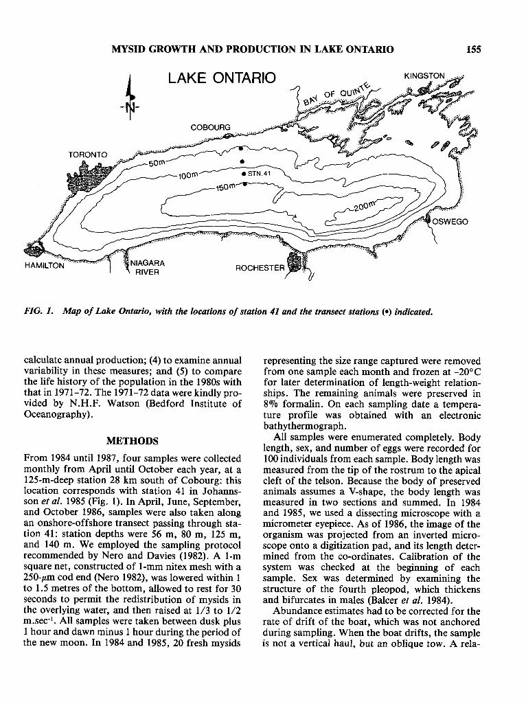
FIG. 1. Map of Lake Ontario, with the locations of station 41 and the transect stations (e) indicated.

calculate annual production; (4) to examine annualvariability in these measures; and (5) to comparethe life history of the population in the 1980s withthat in 1971-72. The 1971-72 data were kindly pro­vided by N.H.F. Watson (Bedford Institute ofOceanography).

METHODS

From 1984 until 1987, four samples were collectedmonthly from April until October each year, at a125-m-deep station 28 km south of Cobourg: thislocation corresponds with station 41 in Johanns­son et al. 1985 (Fig. 1). In April, June, September,and October 1986, samples were also taken alongan onshore-offshore transect passing through sta­tion 41: station depths were 56 m, 80 m, 125 m,and 140 m. We employed the sampling protocolrecommended by Nero and Davies (1982). A I-msquare net, constructed of I-mm nitex mesh with a250-p.m cod end (Nero 1982), was lowered within 1to 1.5 metres of the bottom, allowed to rest for 30seconds to permit the redistribution of mysids inthe overlying water, and then raised at 1/3 to 1/2m.sec- I

• All samples were taken between dusk plus1 hour and dawn minus 1 hour during the period ofthe new moon. In 1984 and 1985, 20 fresh mysids

representing the size range captured were removedfrom one sample each month and frozen at -20°Cfor later determination of length-weight relation­ships. The remaining animals were preserved in8070 formalin. On each sampling date a tempera­ture profile was obtained with an electronicbathythermograph.

All samples were enumerated completely. Bodylength, sex, and number of eggs were recorded for100 individuals from each sample. Body length wasmeasured from the tip of the rostrum to the apicalcleft of the telson. Because the body of preservedanimals assumes a V-shape, the body length wasmeasured in two sections and summed. In 1984and 1985, we used a dissecting microscope with amicrometer eyepiece. As of 1986, the image of theorganism was projected from an inverted micro­scope onto a digitization pad, and its length deter­mined from the co-ordinates. Calibration of thesystem was checked at the beginning of eachsample. Sex was determined by examining thestructure of the fourth pleopod, which thickensand bifurcates in males (Balcer et al. 1984).

Abundance estimates had to be corrected for therate of drift of the boat, which was not anchoredduring sampling. When the boat drifts, the sampleis not a vertical haul, but an oblique tow. A rela-

156 O. JOHANNSSON

tionship was developed empirically between therate of drift and wind speed. Knowing the timetaken to raise the net and the wind speed, the dis­tance drifted during the tow could be calculated.The pathlength of the net was equal to the hypote­nuse of the triangle formed by the station depthand distance drifted during the sample. Knowingthe pathlength, the actual volume of water sam­pled could be calculated and abundance correctedto a m2 basis. Filtering rate was assumed to be100070, a reasonable assumption considering thecoarseness of the mesh.

The effect of depth on the abundance of mysidsalong the onshore-offshore transect was assessedwithin each sampling period with one way analysisof variance. The similarity of the size-frequencydistributions were analyzed with the G-Test (Sokaland Rohlf 1969).

Seasonal patterns of growth of the mysid popu­lation at station 41 were examined by followingcohort development. In order to construct size­frequency histograms for each sampling period,total sample size-frequency distributions were cal­culated for each of the four replicates, and thenumber of mysids in each I-mm size class aver­aged. Mean cohort size was calculated as the aver­age size of an individual in the most populated sizeclasses. If the numbers in the two dominant sizecategories were approximately equal, only two cat­egories were used. Otherwise the peak and twoadjacent categories were employed.

Growth and reproduction were related to thetemperature cycle in the hypolimnion. Tempera­ture data, collected from the 80-140 m depth stra­tum from the center of the lake, were obtainedfrom the Star File Data Bank at the Canada Centrefor Inland Waters (Burlington, Ontario) for theyears 1966-1973 and 1984-1987. The data for eachyear were averaged by month, and then the datafor each month were averaged across years to pro­duce a composite picture of the temperature cycle.

Length-weight relationships were determined foreach month in 1984 and 985. Frozen animals wereplaced in preweighed aluminum dishes, measuredunder a dissecting microscope both to the cleft inthe telson and to the tip of the telson, and dried at60°C to constant weight for 24 h. After coolingthey were reweighed using a Mettler M3 balancewith an accuracy of 0.001 mg. The length andweight data were transformed using natural loga­rithms and the possibilities of seasonal and annualdifferences in the length-weight relationship wereinvestigated with analysis of co-variance.

Annual production was estimated from Octoberto October using the size-frequency method devel­oped by Menzies (1980), a modification of theHynes method. Biomass lost between size classes issummed over the year.

Production = Ej=il (Nj - Nj + 1) x (WjWj + 1)112

and Nj = iiij x PiP. x 365/CPI

where i = number of size categories, Nj = thenumber of mysids that developed into size category'j' in a year, Wj = mean weight of mysids in the jthcategory, iij = mean number of mysids in category'j', Pe = estimated proportion of the life cyclespent in the jth category (IIi), Pa = actual propor­tion of the life cycle spent in the jth category, andCPI = cohort production interval in days fromhatching to reaching the largest size class.

In studying the sensitivity of production esti­mates calculated by this technique, Iversen andDall (1980) found that the size-frequency methodprovided realistic estimates of production if actualgrowth patterns were used, if the population weresampled more than 10 times per cohort productioninterval, and if more than 10 size categories wereemployed. These conditions were met in thepresent study. Confidence intervals were calculatedaccording to Krueger and Martin (1980).

N.H.F. Watson, G.F. Carpenter, and E.L. Man­sey collected mysids monthly from 50 stations inLake Ontario from April 1972 until February1973, and in April, August, and October 1971.They used a I-m2

, 505-J.tm mesh net, raised at1 m.sec-1 from a drifting boat. The more rapidascent used in the 1970s, 1 m.sec-1 as comparedwith 0.3 m.sec- I , helped compensate for drift.Extrapolating from 1984-1987 conditions, abun­dance, corrected for drift, would generally be80-100% of the observed estimate, and in theworst case, 60%. Size-frequency distributions wereconstructed for each month: only those stationsgreater than 60 m in depth which had been sampledat night were included in the analysis. Abundancewas estimated from stations between 100 and 135m, a depth range bracketing that at station 41.

RESULTS

Temperature Cycle in the Hypolimnion

Temperature in the 80-140 m depth stratum fluctu­ated out of phase with the epilimnion, reaching amaximum of 4.50°C in December, after the warm

MYSID GROWTH AND PRODUCTION IN LAKE ONTARIO 157

197119721984

1986

19871.J--~ ---- I

" '. I I, , .. I, • To ',(~. ~""":J:•..~.. • • 1985

....s;J: 1984

500

1000

o.sUJ 0 +--,-----,--,----r--,-----,---() A M J J A SZ 2000«oz::J~ 1500

2000A)

1500

1000

'"E 500

57 3

90-

9 9 9 10Q. 4

W 7a: 3

=> 5!;j: 3 8a: 0wCl.::Ewf- 2

0.8

F M A M J A S 0 N D

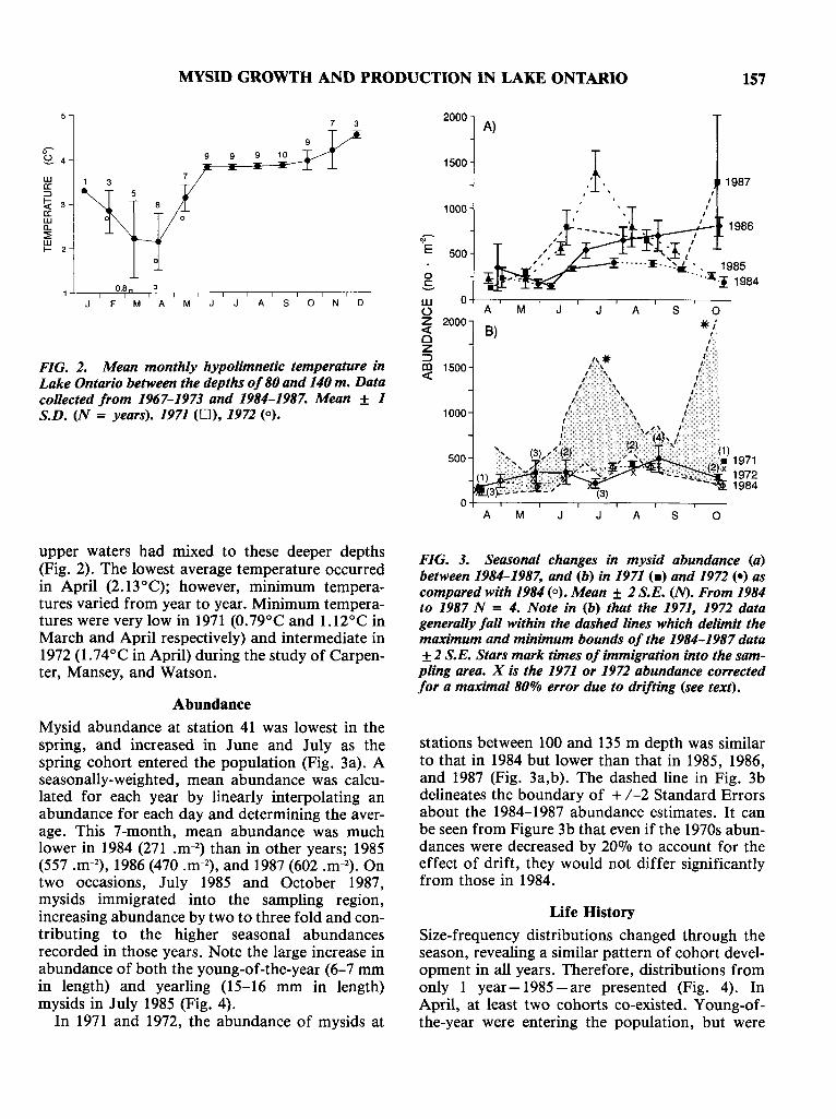
FIG. 2. Mean monthly hypolimnetic temperature inLake Ontario between the depths of80 and 140 m. Datacollected from 1967-1973 and 1984-1987. Mean ± 1S.D. (N = years). 1971 (0), 1972 (0).

0+----,----,--,---,.---,---.----A M J J A S a

upper waters had mixed to these deeper depths(Fig. 2). The lowest average temperature occurredin April (2. 13°C); however, minimum tempera­tures varied from year to year. Minimum tempera­tures were very low in 1971 (0.79°C and 1.12°C inMarch and April respectively) and intermediate in1972 (1.74°C in April) during the study of Carpen­ter, Mansey, and Watson.

Abundance

Mysid abundance at station 41 was lowest in thespring, and increased in June and July as thespring cohort entered the population (Fig. 3a). Aseasonally-weighted, mean abundance was calcu­lated for each year by linearly interpolating anabundance for each day and determining the aver­age. This 7-month, mean abundance was muchlower in 1984 (271 .m-2

) than in other years; 1985(557 .m-2

), 1986 (470 .m-2), and 1987 (602 .m-2). Ontwo occasions, July 1985 and October 1987,mysids immigrated into the sampling region,increasing abundance by two to three fold and con­tributing to the higher seasonal abundancesrecorded in those years. Note the large increase inabundance of both the young-of-the-year (6-7 mmin length) and yearling (15-16 mm in length)mysids in July 1985 (Fig. 4).

In 1971 and 1972, the abundance of mysids at

FIG. 3. Seasonal changes in mysid abundance (a)between 1984-1987, and (b) in 1971 (_) and 1972 (e) ascompared with 1984 (0). Mean ± 2 S.E. (N). From 1984to 1987 N = 4. Note in (b) that the 1971, 1972 datagenerally fall within the dashed lines which delimit themaximum and minimum bounds of the 1984-1987 data±2 S.E. Stars mark times of immigration into the sam-

pling area. X is the 1971 or 1972 abundance correctedfor a maximal 80% error due to drifting (see text).

stations between 100 and 135 m depth was similarto that in 1984 but lower than that in 1985, 1986,and 1987 (Fig. 3a,b). The dashed line in Fig. 3bdelineates the boundary of + /-2 Standard Errorsabout the 1984-1987 abundance estimates. It canbe seen from Figure 3b that even if the 1970s abun­dances were decreased by 20070 to account for theeffect of drift, they would not differ significantlyfrom those in 1984.

Life History

Size-frequency distributions changed through theseason, revealing a similar pattern of cohort devel­opment in all years. Therefore, distributions fromonly 1 year-1985-are presented (Fig. 4). InApril, at least two cohorts co-existed. Young-of­the-year were entering the population, but were

158 O. JOHANNSSON

FIG. 4. Seasonal size-frequency distributions ofmysids at station 41 in 1985 and at all stations > 60 mdepth, sampled at night, in 1972.

mately 10 mm by the end of October. It was impos­sible to follow the l-year-old cohort past the end ofAugust, by which time these mysids were 14-16mm in length. A few very large individuals, greaterthan 17 mm, were observed at all times.

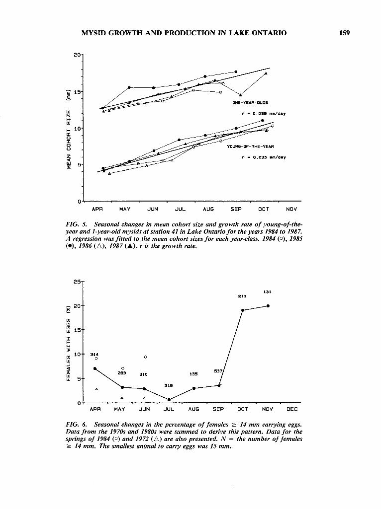
Growth rates were determined from plots ofcohort mean size versus date (Fig. 5). Rates differedseasonally, but remained similar within seasonsacross years. A regression was fitted to mean cohortsize in each period to determine the average1984-1987 rate of growth (Fig. 5). During the firstsummer (April until October) young-of-the-yearmysids grew at 0.035 mm.d- I (r = 0.95, p < 0.001).Growth over the winter (15 October-15 April)slowed to 0.012 mm.d-1• During their second sum­mer, mysids grew at 0.029 mm.d-1 (r = 0.86, p <0.001). Due to diminishing numbers, their growthcould not be followed past the end of August.

Recruitment was not strictly synchronous,although distinct cohorts could be followed.Young entered the population from before April,our earliest sampling period, into June. A few weresometimes observed in later months. The principalreproductive period started in October when thepercentage of females ~ 14 mm in length, whichwere carrying eggs, jumped from less than 5070 toapproximately 20070 (Fig. 6). Because so fewfemales carrying eggs were observed on anyoneday and because the pattern of reproduction wassimilar across years, the data from all years (1971,1972, 1984-1987) were summed by month to pro­duce this figure. Only in 1984 were more than 5070of females ~ 14 mm, carrying eggs in April, May,and June. Shea and Makarewicz (1989) alsoobserved females carrying eggs in May and June1984 at their south-shore station in Lake Ontario.

Cohort development is not as clear in the 1972size-frequency distributions as it was in the 1980s(Fig. 4). Recruitment of young to the populationoccurred in all months in spite of the low number ofegg-carrying females observed from April untilOctober (Fig. 6). The size frequency distribution of21 June was out of step with all the others, andshowed an influx of newly hatched individualswhich were not seen in the July samples. If Junewere ignored, one can roughly follow a cohortwhich was approximately 4.5 mm in May, 5.2 mmin mid-July, 9.6 mm in early September, and 10.3mm in November. The l-year-old cohort can beseen in April, but is indistinguishable thereafter.The shoulder of that cohort reached 15 mm in mid­July. There appears to be a relative decrease inlarger size classes after that time.

April 30

September 5

1972

4 6 8 10 12 14 16 1820

80

40

80

BODY LENGTH (mm)

April 12

1985

4 6 8101214161820

80

160

still small, approximately 4.5 mm in length. Themajority of the previous year's cohort were 11 to14 mm long. Some larger individuals were alsopresent. Young were not well sampled until theywere 6-7 mm long. Consequently, maximum abun­dances of the new cohort were not observed untilJune or July. Young-of-the-year grew to approxi-

'l'E

ci.sw()z«oz::JIn«

MYSID GROWTH AND PRODUCTION IN LAKE ONTARIO 159

20

E 15§

ONE-YEAR-OLOS

UJ r • 0.029 mm/aeyNH1JJ

~10

a:0J:0U

Z r • 0.035 mm/aey-<UJ 5:::E

O+-----..,------r---.,....-----..,---....,----..------,.---APR MAY JUN JUL AUG SEP OCT NOV

FIG. 5. Seasonal changes in mean cohort size and growth rate of young-of-the­year and l-year-old mysids at station 41 in Lake Ontario for the years 1984 to 1987.A regression was fitted to the mean cohort sizes for each year-class. 1984 (0), 1985(e), 1986 (6), 1987 (.). r is the growth rate.

25

131211

~ 20!!1JJt!lt!l 15UJ

J:~H3:

1JJ10 314

UJ0

.J-<:::EUJ

5lL

I>.

I>.

0APR MAY JUN JUL AUG SEP OCT NOV DEC

FIG. 6. Seasonal changes in the percentage of females;::: 14 mm carrying eggs.Data from the 1970s and 1980s were summed to derive this pattern. Data for thesprings of 1984 (0) and 1972 (6) are also presented. N = the number of females;::: 14 mm. The smallest animal to carry eggs was 15 mm.

160 O. JOHANNSSON

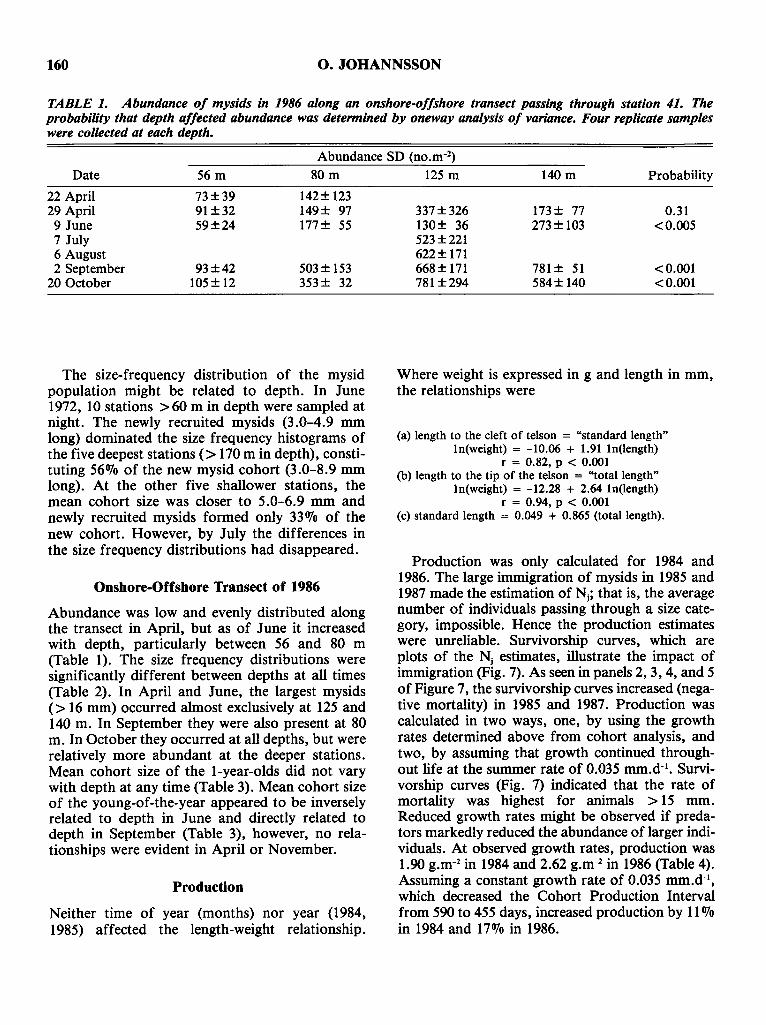
TABLE 1. Abundance of mysids in 1986 along an onshore-offshore transect passing through station 41. Theprobability that depth affected abundance was determined by oneway analysis of variance. Four replicate sampleswere collected at each depth.

Abundance SD (no.m-2)

Date 56m 80m 125 m 140 m Probability

22 April 73±39 142± 12329 April 91±32 149± 97 337±326 173± 77 0.319 June 59±24 177± 55 130± 36 273± 103 <0.0057 July 523±2216 August 622± 1712 September 93±42 503± 153 668± 171 781 ± 51 <0.001

20 October 105± 12 353± 32 781 ±294 584± 140 <0.001

The size-frequency distribution of the mysidpopulation might be related to depth. In June1972, 10 stations >60 m in depth were sampled atnight. The newly recruited mysids (3.0-4.9 mmlong) dominated the size frequency histograms ofthe five deepest stations (> 170 m in depth), consti­tuting 56010 of the new mysid cohort (3.0-8.9 mmlong). At the other five shallower stations, themean cohort size was closer to 5.0-6.9 mm andnewly recruited mysids formed only 33010 of thenew cohort. However, by July the differences inthe size frequency distributions had disappeared.

Onshore-Offshore Transect of 1986

Abundance was low and evenly distributed alongthe transect in April, but as of June it increasedwith depth, particularly between 56 and 80 m(Table 1). The size frequency distributions weresignificantly different between depths at all times(Table 2). In April and June, the largest mysids(> 16 mm) occurred almost exclusively at 125 and140 m. In September they were also present at 80m. In October they occurred at all depths, but wererelatively more abundant at the deeper stations.Mean cohort size of the l-year-olds did not varywith depth at any time (Table 3). Mean cohort sizeof the young-of-the-year appeared to be inverselyrelated to depth in June and directly related todepth in September (Table 3), however, no rela­tionships were evident in April or November.

Production

Neither time of year (months) nor year (1984,1985) affected the length-weight relationship.

Where weight is expressed in g and length in mm,the relationships were

(a) length to the cleft of telson = "standard length"In(weight) = -10.06 + 1.91 In(length)

r = 0.82, p < 0.001(b) length to the tip of the telson = "total length"

In(weight) = -12.28 + 2.64 In(length)r = 0.94, p < 0.001

(c) standard length = 0.049 + 0.865 (total length).

Production was only calculated for 1984 and1986. The large immigration of mysids in 1985 and1987 made the estimation of Nj ; that is, the averagenumber of individuals passing through a size cate­gory, impossible. Hence the production estimateswere unreliable. Survivorship curves, which areplots of the Nj estimates, illustrate the impact ofimmigration (Fig. 7). As seen in panels 2, 3, 4, and 5of Figure 7, the survivorship curves increased (nega­tive mortality) in 1985 and 1987. Production wascalculated in two ways, one, by using the growthrates determined above from cohort analysis, andtwo, by assuming that growth continued through­out life at the summer rate of 0.035 mm.d-1

• Survi­vorship curves (Fig. 7) indicated that the rate ofmortality was highest for animals > 15 mm.Reduced growth rates might be observed if preda­tors markedly reduced the abundance of larger indi­viduals. At observed growth rates, production was1.90 g.m-2 in 1984 and 2.62 g.m-2 in 1986 (Table 4).Assuming a constant growth rate of 0.035 mm.d-1,

which decreased the Cohort Production Intervalfrom 590 to 455 days, increased production by 11010in 1984 and 17010 in 1986.

MYSID GROWTH AND PRODUCTION IN LAKE ONTARIO 161

TABLE 2. Effect of depth on the relative distribution of mysids in three size classas: (A) <= 8.99 mm, (B) 9.00-15.99 mm, (C) >= 16.00 mm. The size frequency distributions were compared with the G-Test (Sokal and Rohlf1969).

Relative Composition (070) G-Test ResultDate Group 56 m 80m 125 m 140 m (Probability)

29 April A 88.7 93.2 74.1 54.7 683B 11.1 6.6 23.5 35.1 ( <0.001)C 0.2 0.2 2.3 10.3

9 June A 93.7 80.4 57.4 65.0 1209B 6.1 18.5 39.4 31.3 ( <0.001)C 0.2 1.1 3.2 3.7

2 September A 67.8 51.8 28.7 52.8 1030B 31.5 42.0 64.0 39.8 ( <0.001)C 0.7 6.3 7.3 7.4

20 October A 41.8 29.8 23.4 30.8 2139B 57.8 69.6 69.4 67.1 ( <0.001)C 0.4 2.6 7.2 2.1

DISCUSSION

Life History and Growth

Mysids in the Great Lakes generally live on thebottom during the day and in the water column atnight. However, in the deeper regions, pelagic pop­ulations have been observed during the day in LakeMichigan (Robertson et al. 1968). Mysids migrateinto the water column when light levels fall below1,000 photons.mm-2.s-1 of green light (Beeton

TABLE 3. Effect of depth on cohort mean size. N.D.indicates that cohort mean size could not be distin-guished. A '-' indicates that < 1% ofindividuals were inthat size range.

Mean Size (mm)

Date Cohort 56 m 80m 125 m 140 m

29 April 1 4.39 4.30 4.30 4.372 12.38 11.85 13.36 12.483 n.d. n.d.

9 June 1 5.89 5.67 5.36 4.642 13.94 13.62 13.64 13.443 n.d. n.d. n.d.

2 September 1 7.52 8.06 9.57 8.422 n.d. n.d. n.d. n.d.3 n.d. n.d. n.d.

20 October 1 10.49 9.60 10.02 9.482 n.d. n.d. n.d. n.d.3 n.d. n.d. n.d.

1959, Moen and Langeland 1989). Benthic sledshave been used to sample mysids during the day(e.g., Reynolds and DeGraeve 1972); however, it isdifficult to determine the area sampled with thistechnique. On the recommendation of Grossnickleand Morgan (1979) and Nero and Davies (1982),others have sampled at night using vertical nettows. Grossnickle and Morgan (1979) found thatnighttime abundance estimates were greater thandaytime estimates, at least at stations up to 50 m indepth. At deeper stations abundances were similarbetween daytime sled samples and vertical nethauls but the size distributions differed: morelarger organisms were found in the sled samples(Grossnickle and Morgan 1979). A tendency forlarger organisms to remain closer to the bottomhas also been observed by Moen and Langeland(1989). Shea and Makarewicz (1989), in their 1984study of two stations in southern Lake Ontario,took benthic sled tows at night at the same time astheir vertical net hauls, and found that approxi­mately 1070 of the population remained on the bot­tom at the 100 m stations. Their data confirm theearlier observation that abundance was accuratelyestimated by vertical net hauls. If that 1% werecomposed only of larger organisms it could, onoccasion, increase the number of larger mysidsobserved by 50% (Table 2). The main impact ofthis error would be in the production estimates. Itwould be unlikely to affect the life history andgrowth rate determinations.

Mysis relicta required 2 years to complete its life

162 O. JOHANNSSON

7.0 7.0

6.0

~6.0 • e..--------- ••

~5.0 5.0 •

1983-198419:4-1985

1984-19854.0 4.0

3.0 3.0

2.0 2.0

1.0 to1984 Cohort 1985 Cohort

0 03 5 7 9 11 13 15 17 19 21 3 5 7 9 11 13 15 17 19 21

2.0

1.5 jo 19~7 C?ho~t , I I I I I I

3 5 7 9 11 13 15 17 19 213 5 7 9 11 13 15 17 19 21

7.0

~ . 6.0 ~1985-1986 5.0 1986-1987

4.0

3.0

1986 Cohort1.0

7.0

2.0

4.0

6.0

3.0

5.0

7.0

6.0

5.0

~4.0

3.0

- 2.0N

IE to0 1983 CohortC 0- 11 13 15 17 19 21

'--'Z

Z.....J

BODY LENGTH (mm)

FIG. 7. Cohort survivorship curves for station 41 in Lake Ontario, 1984-1987. ~ = the number of individualspassing through size category j in 1 year. The year started and ended with the late October sample. Circled areas showincreases in cohort abundance due to immigration.

Observed Continuous PercentYear Growth Growth Increase

Production (SD)(mg'm-2'yr1)

TABLE 4. Annual production of Mysis reUcta, calcu­lated from October to October by the size-frequencymethod (Menzies 1980), under two growth scenarios: (a)growth as observed by cohort analysis, (b) continuousgrowth at 0.035 mm.trl

•

cycle from egg to reproducing adult in LakeOntario. Breeding started in October (Fig. 6). Wecalculated development times for eggs in LakeOntario by using Morgan's (1980) developmentrate of 128 days at 4.5°C as a baseline, assuming a

QlO of 2, and applying these conditions to the sea­sonal temperature regime in the hypolimnion (Fig.2). Morgan (1980) found that his development ratewas related to Berrill's (1969), for mysid eggs atI-3°C, by a QlO of approximately 2. Eggs fertilizedby the end of October would have hatched by 18March (Fig. 8). Young are 3.5 to 4.0 mm totallength (or 3.1-3.5 mm standard length) when born(Berrill 1969, Lasenby and Langford 1972). At agrowth rate of 0.035 mm.d-1 they would be approx­imately 4.4 mm long in mid- to late April. Thisagrees closely with the observed mean cohort sizeof 4.26 mm on 25 April, calculated from the equa­tion for growth during the first summer (Fig. 5).The size range of this cohort spans several mm,indicating that reproduction took place over aperiod of several months. In 1984 and 1985, thecohort encompassed the 5 to 9 mm range in mid­June. To produce this range, breeding would havetaken place from the beginning of September to

11 07017%

2,117 (88)

3,072 (222)

1,899 (69)

2,620 (236)1984

1986

MYSID GROWTH AND PRODUCTION IN LAKE ONTARIO 163

1.0I-ZlU~[L0 0.8JlU>lUC

U....Z0>-a:m

0.4~lU

lU>....l-e(J::J~::JU

SEP OCT NOV DEC .JAN FE8 MAR APR MAY .JUL AUB

FIG. 8. Egg development times assuming a QIO of 3.4 and an egg development time of 118 days at 4.5°C (Morgan1980). The patterns of development for a series of fertilization dates are plotted for a normal (A) and exceptionallycold (6 - 1971) winter.

the end of November the previous autumn (Fig. 8).In 1986 and 1987, the range was smaller, 4 to 7 or 8mm by the end of June: breeding, therefore,should have occurred from mid-October until theend of December the previous years. We have nosamples from September 1984 to test the 1985"projections"; however, the proportion of femalescarrying eggs in October 1984 was greater than theproportions in 1985 or 1986: 19.9% as comparedwith 8.2070 and 2.7%, respectively. As predicted forthe autumns of 1985 and 1986, reproductive activ­ity was just starting in October. These calculationsmay have overestimated the length of the repro­ductive period because they assumed that all ani­mals grew at one rate, 0.035 mm.d- I

, but they mayhave underestimated it by not taking into accountthe possibility of lower growth rates in the coldermonths. Both effects would be small and tend tocancel out each other. The spring cohort did notreach sexual maturity by the first autumn. Repro­duction occurred in the cohort which had beenborn approximately 18 months earlier. Conse-

quently, the maximum number of co-existingcohorts occurred in April when the populationconsisted of newly born young-of-the-year, imma­ture l-year-old and reproductively-spent, and 2­year-old individuals. Shea and Makarewicz (1989)saw similar size-frequency distributions at theirsouth shore station in 1984 as we saw at station 41and also concluded that Mysis relicta had a 2-yearlife cycle in Lake Ontario. They divided recruit­ment into early and late spring cohorts whichblended by the following spring. Such divisionseems artificial because reproduction has not beenshown to be highly synchronous, and becauserecruitment in other studies is not synchronous butbroadly based (e.g., Lasenby and Langford 1972­Char Lake, Stony Lake; Reynolds and DeGraeve1972-Lake Michigan; Morgan 1980-LakeTahoe, Emerald Bay).

The reproductive period of the mysid populationin Lake Ontario was more distinct in the 1980sthan in 1971 or 1972. Both earlier and later studiesindicated that Mysis relicta required 2 years to

164 O. JOHANNSSON

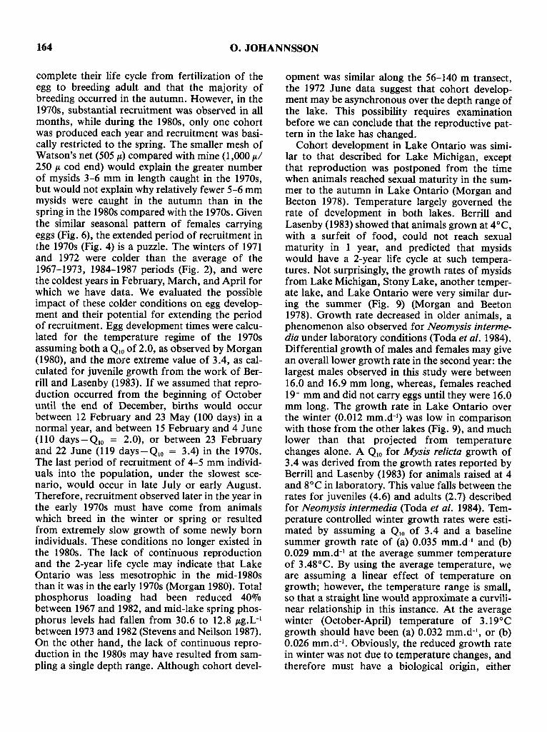
complete their life cycle from fertilization of theegg to breeding adult and that the majority ofbreeding occurred in the autumn. However, in the1970s, substantial recruitment was observed in allmonths, while during the 1980s, only one cohortwas produced each year and recruitment was basi­cally restricted to the spring. The smaller mesh ofWatson's net (505 IL) compared with mine (1,000 ILl250 IL cod end) would explain the greater numberof mysids 3-6 mm in length caught in the 1970s,but would not explain why relatively fewer 5-6 mmmysids were caught in the autumn than in thespring in the 1980s compared with the 1970s. Giventhe similar seasonal pattern of females carryingeggs (Fig. 6), the extended period of recruitment inthe 1970s (Fig. 4) is a puzzle. The winters of 1971and 1972 were colder than the average of the1967-1973, 1984-1987 periods (Fig. 2), and werethe coldest years in February, March, and April forwhich we have data. We evaluated the possibleimpact of these colder conditions on egg develop­ment and their potential for extending the periodof recruitment. Egg development times were calcu­lated for the temperature regime of the 1970sassuming both a QIO of 2.0, as observed by Morgan(1980), and the more extreme value of 3.4, as cal­culated for juvenile growth from the work of Ber­rill and Lasenby (1983). If we assumed that repro­duction occurred from the beginning of Octoberuntil the end of December, births would occurbetween 12 February and 23 May (100 days) in anormal year, and between 15 February and 4 June(110 days - QIO = 2.0), or between 23 Februaryand 22 June (119 days-QIO = 3.4) in the 1970s.The last period of recruitment of 4-5 mm individ­uals into the population, under the slowest sce­nario, would occur in late July or early August.Therefore, recruitment observed later in the year inthe early 1970s must have come from animalswhich breed in the winter or spring or resultedfrom extremely slow growth of some newly bornindividuals. These conditions no longer existed inthe 1980s. The lack of continuous reproductionand the 2-year life cycle may indicate that LakeOntario was less mesotrophic in the mid-1980sthan it was in the early 1970s (Morgan 1980). Totalphosphorus loading had been reduced 40010between 1967 and 1982, and mid-lake spring phos­phorus levels had fallen from 30.6 to 12.8 ILg.L-1between 1973 and 1982 (Stevens and Neilson 1987).On the other hand, the lack of continuous repro­duction in the 1980s may have resulted from sam­pling a single depth range. Although cohort devel-

opment was similar along the 56-140 m transect,the 1972 June data suggest that cohort develop­ment may be asynchronous over the depth range ofthe lake. This possibility requires examinationbefore we can conclude that the reproductive pat­tern in the lake has changed.

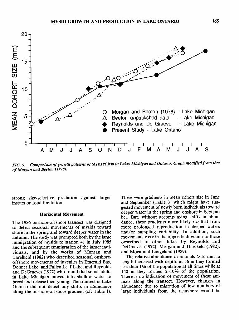
Cohort development in Lake Ontario was simi­lar to that described for Lake Michigan, exceptthat reproduction was postponed from the timewhen animals reached sexual maturity in the sum­mer to the autumn in Lake Ontario (Morgan andBeeton 1978). Temperature largely governed therate of development in both lakes. Berrill andLasenby (1983) showed that animals grown at 4°C,with a surfeit of food, could not reach sexualmaturity in 1 year, and predicted that mysidswould have a 2-year life cycle at such tempera­tures. Not surprisingly, the growth rates of mysidsfrom Lake Michigan, Stony Lake, another temper­ate lake, and Lake Ontario were very similar dur­ing the summer (Fig. 9) (Morgan and Beeton1978). Growth rate decreased in older animals, aphenomenon also observed for Neomysis interme­dia under laboratory conditions (Toda et al. 1984).Differential growth of males and females may givean overall lower growth rate in the second year: thelargest males observed in this study were between16.0 and 16.9 mm long, whereas, females reached19+ mm and did not carry eggs until they were 16.0mm long. The growth rate in Lake Ontario overthe winter (0.012 mm.d-1) was low in comparisonwith those from the other lakes (Fig. 9), and muchlower than that projected from temperaturechanges alone. A QIO for Mysis relicta growth of3.4 was derived from the growth rates reported byBerrill and Lasenby (1983) for animals raised at 4and 8°C in laboratory. This value falls between therates for juveniles (4.6) and adults (2.7) describedfor Neomysis intermedia (Toda et af. 1984). Tem­perature controlled winter growth rates were esti­mated by assuming a QIO of 3.4 and a baselinesummer growth rate of (a) 0.035 mm.d-1 and (b)0.029 mm.d-1at the average summer temperatureof 3.48°C. By using the average temperature, weare assuming a linear effect of temperature ongrowth; however, the temperature range is small,so that a straight line would approximate a curvili­near relationship in this instance. At the averagewinter (October-April) temperature of 3.19°Cgrowth should have been (a) 0.032 mm.d-1, or (b)0.026 mm.d-1• Obviously, the reduced growth ratein winter was not due to temperature changes, andtherefore must have a biological origin, either

20

MYSID GROWTH AND PRODUCTION IN LAKE ONTARIO 165

5

....-EE-- 15WNC/)

.-a: 10o:::co()

z«w~

o Morgan and Beeton (1978) - Lake Michigan~ Beeton unpublished data - Lake Michigan• Reynolds and De Graeve - Lake Michigan• Present Study - Lake Ontario

A M J J A SON D J F M A M J J A S

FIG. 9. Comparison ofgrowth patterns of Mysis relicta in Lakes Michigan and Ontario. Graph modified from thatof Morgan and Beeton (1978).

strong size-selective predation against largerinstars or food limitation.

Horizontal Movement

The 1986 onshore-offshore transect was designedto detect seasonal movements of mysids towardshore in the spring and toward deeper water in theautumn. The study was prompted both by the largeimmigration of mysids to station 41 in July 1985and the subsequent emmigration of the larger indi­viduals, and by the works of Morgan andThrelkeld (1982) who described seasonal onshore­offshore movements of juveniles in Emerald Bay,Donner Lake, and Fallen Leaf Lake, and Reynoldsand DeGraeves (1972) who found that some adultsin Lake Michigan moved into shallow water tobreed and release their young. The transect in LakeOntario did not detect any shifts in abundancealong the onshore-offshore gradient (cf. Table 1).

There were gradients in mean cohort size in Juneand September (Table 3) which might have sug­gested movement of newly born individuals towarddeeper water in the spring and onshore in Septem­ber. But, without accompanying shifts in abun­dance, these gradients more likely resulted frommore prolonged reproduction in deeper watersand/or sampling variability. In addition, suchmovements were in the opposite direction to thosedescribed in other lakes by Reynolds andDeGraeves (1972), Morgan and Threlkeld (1982),and Moen and Langeland (1989).

The relative abundance of animals > 16 mm inlength increased with depth: at 56 m they formedless than 10,10 of the population at all times while at140 m they formed 2-10% of the population.There is no indication of movement of these ani­mals along the transect. However, changes inabundance due to migration of low numbers oflarge individuals from the nearshore would be

166 O. JOHANNSSON

swamped by the larger number of such animals inthe offshore. The relatively lower percentage oflarge individuals at shallower stations may be dueto higher mortality rates as easily as offshoremigration. Movement into the nearshore would bemore easily recognized, but was not seen. Wheremigration has been observed, physical factors havesometimes been involved. Both low oxygen andhigher temperatures have caused mysids to migratealong an onshore-offshore gradient (Reynolds andDeGraeve 1972, Moen and Langeland 1989, Sheaand Markarewicz 1989). Light has also been sus­pected (Grossnickle and Morgan 1979). These fac­tors would not be important along the 56-140 mtransect in Lake Ontario. Nor did we see any evi­dence of adults releasing their young in shallowwater before returning to deeper regions them­selves, as witnessed by Reynolds and DeGraeve(1972), Moen and Langeland (1989), and in a vari­ate, Morgan and Threlkeld (1982).

The immigration of mysids observed in 1985 atstation 41 could not be explained by onshore­offshore migrations and was not observed again in1986; however, it was seen again in October 1987.We suspect that upwelling events are responsiblefor the mass translocation of large numbers ofmysids. Both immigration events were preceded bya period of strong northwest winds during the pre­vious month. These strong winds were notobserved at any other time during the study. Suchwinds push epilimnetic water to the southeastshore of the lake and cause hypolimnetic water tomove toward the northeast (Simons and Schwert­zer 1987). This hypolimnetic flow would bringmysids from deeper regions of the lake toward sta­tion 41. Because mysid density increases withdepth (Carpenter et af. 1974, Grossnickle and Mor­gan 1979), the influx of mysids into the shallowerregions would be considerable: densities increasedby more than 100070 at station 41. Mass movementsof mysids have been mentioned in connection withupwelling events in Lake Michigan (Reynolds andDeGraeve 1972) and Lake Ontario (Shea andMakarewicz 1989) where mysids were brought intoshallow unpopulated or sparsely populatedregions. These observations confirm that waterflow associated with upwelling events can trans­port mysids a fair distance.

Production

Our production estimates of 1.90 to 2.62 g.m-Z.yr-I

for a station at 125 m depth are comparable to those

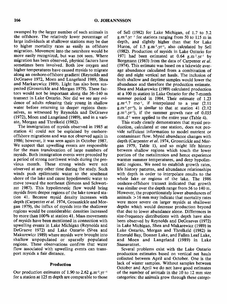
of Sell (1982) for Lake Michigan, of 1.7 to 3.2g.m-Z.yr-I for stations ranging from 50 to 115 mindepth, and slightly higher than that for LakeHuron, of 1.5 g.m-2.yrl , also calculated by Sell(1982). Production of mysids in Lake Ontario for1971 had been estimated at 0.64 g.m-2.yrl byBorgmann (1983) from the data of Carpenter et af.(1974). This estimate was based on a lakewide aver­age abundance calculated from a combination ofday and night vertical net hauls. The inclusion ofboth shallow and daytime samples would lower theabundance and therefore the production estimate.Shea and Makarewicz (1989) calculated productionat a 100 m station in Lake Ontario for the 7-monthsummer period in 1984. Their estimate of 1.23g.m-2.7 mo-1, if interpolated to a year (2.11g.m-2.yr1), is similar to that at station 41 (2.12g.m-2.yrl), if the summer growth rate of 0.035mm.d- I were applied to the entire year (Table 4).

This study clearly demonstrates that mysid pro­duction, calculated at one station, does not pro­vide sufficient information to model nutrient orcontaminant flow. Mysid abundance changes withdepth (Carpenter et af. 1974, Grossnickle and Mor­gan 1979, Table 1), and so might life historybetween shallow regions which touch the lowerportion of the metalimnion and hence experiencewarmer summer temperatures, and deep hypolim­netic regions. We need to establish growth rates,life history patterns, and abundance relationshipswith depth in order to interpolate results to thewhole lake or regions of the lake. The 1986onshore-offshore transect indicated that growthwas similar over the depth range from 56 to 140 m.However, the proportionately lower abundances ofanimals > 16 mm may indicate that mortality rateswere more severe on larger mysids at shallowerdepths which would decrease production beyondthat due to lower abundance alone. Differences insize-frequency distributions with depth have alsobeen observed by Reynolds and DeGraeves (1972)in Lake Michigan, Shea and Makarewicz (1989) inLake Ontario, Morgan and Threlkeld (1982) inEmerald Bay, Donner Lake, and Fallen Leaf Lake,and Moen and Langeland (1989) in LakeSnasavatnet.

Several problems exist with the Lake Ontarioproduction estimates based on vertical net haulscollected between April and October. One is thelack of winter samples. Without samples betweenOctober and April we do not have good estimatesof the number of animals in the 10 to 12 mm sizecategories: the animals grow through these catego-

MYSID GROWTH AND PRODUCTION IN LAKE ONTARIO 167

ries during the winter period. Another problem isthe possibility that net hauls do not adequatelysample larger instars which may be prone to stay­ing on or closer to the bottom (Grossnickle andMorgan 1979). The upper limit of this error can beestimated: if half of the 13 mm mysids grew to19 mm (females) before dying, and the other halfgrew to 17 mm (males) before dying, productionwould have increased by 270/0 in 1984 and 17% in1986. Production would also be underestimated ifwinter growth rates determined from cohort analy­sis were too low, as might occur if mortality rateswere more severe on larger mysids than on inter­mediate ones. The impact of this error can beassessed by assuming that the summer growth rateobserved during the first year applied to the wholelife span. Production, in this case, could beincreased by 11 % in 1984 and 17% in 1986. Thelast source of error is the openness of the system totranslocation of mysids. For this reason, produc­tion could not be calculated in 1985 and 1987. Lessobvious movements of animals may not bedetected and would add to variability in the pro­duction estimate.

ACKNOWLEDGMENTS

We thank Dr. N.H.F. Nelson for the use of hisoriginal mysid data, and Dr. D. Lasenby for com­ments on the manuscript. We also appreciate thehelpfulness of the Captains and crews of theC.S.S. Bayfield, of Technical Operations person­nel, and of a number of students and technicians incollecting samples on many a dark night.

REFERENCES

Balcer, M. D., Korda, N. L., and Dodson, S. 1.1984.Zooplankton of the Great Lakes. A guide to the iden­tification and ecology of the common crustacean spe­cies. Madison, Wisconsin: The University of Wiscon­sin Press.

Beeton, A. M. 1959. Photoreception in the opossumshrimp Mysis relicta Loven. Bioi. Bull. 116:204-216.

Berrill, M. 1969. The embryonic behaviour of the mysidshrimp, Mysis relicta. Can. J. Zool. 47:1217-1221.

____ ,and Lasenby, D. C. 1983. Life cycles of thefreshwater mysid shrimp Mysis relicta reared at twotemperatures. Trans. Amer. Fish. Soc. 112:551-553.

Borgmann, U. 1983. Effect of somatic growth andreproduction on biomass transfer up pelagic foodwebs as calculated from particle-size conversion effi­ciency. Can. J. Fish. Aquat. Sci. 40:2010-2018.

Carpenter, G. F., Mansey, E. L., and Watson, N. H. F.1974. Abundance and life history of Mysis relicta in

the St. Lawrence Great Lakes. J. Fish. Res. BoardCan. 31:319-325.

Crowder, L. B. 1986. Ecological and morphologicalshifts in Lake Michigan fishes: glimpses of the ghostof competition past. Environ. Bioi. Fish. 16:147-157.

Evans, D.O., and Loftus, D. H. 1987. Colonization ofinland lakes in the Great Lakes region by rainbowsmelt, Osmerus mordax: their freshwater niche andeffects on indigenous fishes. Can. J. Fish. Aquat.Sci. Suppl. 2 44:249-266.

Grossnickle, N. E., and Morgan, M. D. 1979. Densityestimates of Mysis relicta in Lake Michigan. J. FishRes. Board. Can. 36:694-698.

Iversen, T. M., and Dall, P. 1989. The effect of growthpattern, sampling interval and number of size classeson benthic invertebrate production estimated by thesize-frequency method. Freshwat. Bioi. 22:323-331.

Janssen, J., and Brandt, S. B. 1980. Feeding ecologyand vertical migration of adult alewives (Alosapseudoharengus) in Lake Michigan. Can. J. Fish.Aquat. Sci. 37:177-184.

Johannsson, O. E., Dermott, R. M., Feldkamp, R., andMoore, J. E. 1985. Lake Ontario Long Term Biologi­cal Monitoring Program: Report for 1981 and 1982.Can. Tech. Rep. Fish. Aquat. Sci. No. 1414.

Kraft, C. E., and Kitchell, J. F. 1986. Partitioning offood resources by sculpins in Lake Michigan. Envi­ron. Bioi. Fish. 16:309-316.

Krueger, C. C., and Martin, F. B. 1980. Computationof confidence intervals for the size-frequency(Hynes) method of estimating secondary production.Limnol. Oceanogr. 25:773-777.

Lasenby, D. C., and Langford, R. R. 1972. Growth, lifehistory and respiration of Mysis relicta in an arcticand temperate lake. J. Fish. Res. Board Can.29:1701-1708.

Menzies, C. A. 1980. A note on the Hynes method ofestimating secondary production. Limnol. Oceanogr.25:770-773.

Moen, V., and Langeland, A. 1989. Diurnal vertical andseasonal horizontal distribution patterns of Mysisrelicta in a large Norwegian lake. J. Plank. Res.11:729-745.

Morgan, M. D. 1980. Life history characteristics of twointroduced populations of Mysis relicta. Ecol.61:551-561.

____ , and Beeton, A. M. 1978. Life history andabundance of Mysis relicta in Lake Michigan. J.Fish. Res. Board Can. 35:1165-1170.

____ , and Threlkeld, S. T. 1982. Size dependenthorizontal migration of Mysis relicta. Hydrobiol.93:63-68.

Morsell, J. W., and Norden, C. R. 1968. Food habits ofthe alewife, Alosa pseudoharengus (Wilson), in LakeMichigan. In Proc. 11th Conj. Great Lakes Res., pp.96-102. Internat. Assoc. Great Lakes Res.

168 O. JOHANNSSON

Nero, R. W. 1982. A description of three nets suitablefor estimating the abundance of Mysis relicta. Can.Tech. Rep. Fish. Aquat. Sci. 1046.

____ , and Davies, I. J. 1982. Comparison of twosampling methods for estimating the abundance anddistribution of Mysis relicta. Can. J. Fish. A quat.Sci. 39:349-355.

Reynolds, J. B., and DeGraeve, G. M. 1972. Seasonalpopulation characteristics of the opossum shrimp,Mysis relicta, in southeastern Lake Michigan. InProc. 15th Conj. Great Lakes Res., pp. 117-131.Internat. Assoc. Great Lakes Res.

Robertson, A., Powers, C. F., and Anderson, R. F.1968. Direct observations on Mysis relicta from asubmarine. Limnol. Oceanogr. 13:700-702.

Scott, W. B., and Crossman, E. J. 1973. FreshwaterFishes of Canada. Fish. Res. Board Can. Bull. 184.

Sell, D. W. 1982. Size-frequency estimates of secondaryproduction by Mysis relicta in Lakes Michigan andHuron. Hydrobiol. 93:69-78.

Shea, M. A., and Makarewicz, J. C. 1989. Production,biomass, and trophic interactions of Mysis relicta inLake Ontario. J. Great Lakes Res. 15:223-232.

Simons, T. J., and Schertzer, W. M. 1987. Stratifica­tion, currents and upwelling in Lake Ontario, sum­mer 1982. Can. J. Fish. Aquat. Sci. 44:2047-2058.

Sokal, R. R., and Rohlf, F. J. 1969. Biometry. SanFrancisco: W. H. Freeman and Co.

Stevens, R. J. J., and Neilson, M. A. 1987. Response ofLake Ontario to reductions in phosphorus load,1967-82. Can. J. Fish. Aquat. Sci. 44:2059-2068.

Toda, H., Takahashi, M., and Ichimura, S. 1984. Theeffect of temperature on the post-embryonic growthof Neomysis intermedia Czerniawsky (Crustacea,Mysidacea) under laboratory conditions. J. Plank.Res. 6:647-662.

Wells, L., and Beeton, A. M. 1963. Food of the bloater,Coregonus hoyi, in Lake Michigan. Trans. A mer.Fish. Soc. 92:245-255.

Wojcik, J. A., Evans, M. S., and Jude, D. J. 1986.Food of deepwater sculpin, Myoxocephalus thomp­soni, from southeastern Lake Michigan. J. GreatLakes Res. 12:225-231.

Submitted: 18 December 1990Accepted: 28 November 1991