Life Satisfaction, Income and Personality Theory Eugenio Proto a Aldo Rustichini b a Department of Economics, University of Warwick b Department of Economics, University of Minnesota September 2011 Abstract: Neuroticism is responsible for the decline of happiness with high income and its increase for lower incomes in both SOEP and BHPS datasets. We suggest that the effect is due to the psychological cost of the gap between aspiration and realized income. High income individuals fail to meet expectation, this explains lower increase or decrease of life satis- faction for highly neurotic individuals for higher income levels. Data show a hump-shaped relation between income and life satisfaction, with a bliss point between 250-300K 2005 USD. For highly neurotic this peak occurs at lower income, and disappears for non neurotic individuals. JEL classification: D03; D870; C33. Keywords: Life Satisfaction, Income, Personality Theory, Neuroticism. Acknowledgements The authors thank several coauthors and colleagues for discussions on related research, especially Wiji Arulampalam, Sasha Becker, Gordon Brown, Dick Easterlin, Peter Hammond, Alessandro Iaria, Graham Loomes, Kyoo il Kim, Rocco Macchiavello, Anandi Mani, Fabien Postel- Vinay, Dani Rodrik, Jeremy Smith, Chris Woodruf, Fabian Waldinger. Proto thanks the ESRC (grant RES-074-27-0018); Rustichini thanks the NSF (grant SES-0924896) and ESRC (grant RES-062-23-1385).
Transcript
Life Satisfaction, Income andPersonality Theory
Eugenio Protoa Aldo Rustichinib
aDepartment of Economics, University of WarwickbDepartment of Economics, University of Minnesota
September 2011
Abstract: Neuroticism is responsible for the decline of happiness withhigh income and its increase for lower incomes in both SOEP and BHPSdatasets. We suggest that the effect is due to the psychological cost of thegap between aspiration and realized income. High income individuals failto meet expectation, this explains lower increase or decrease of life satis-faction for highly neurotic individuals for higher income levels. Data show ahump-shaped relation between income and life satisfaction, with a bliss pointbetween 250-300K 2005 USD. For highly neurotic this peak occurs at lowerincome, and disappears for non neurotic individuals.
Acknowledgements The authors thank several coauthors and colleaguesfor discussions on related research, especially Wiji Arulampalam, Sasha Becker,Gordon Brown, Dick Easterlin, Peter Hammond, Alessandro Iaria, GrahamLoomes, Kyoo il Kim, Rocco Macchiavello, Anandi Mani, Fabien Postel-Vinay, Dani Rodrik, Jeremy Smith, Chris Woodruf, Fabian Waldinger.
Proto thanks the ESRC (grant RES-074-27-0018); Rustichini thanks theNSF (grant SES-0924896) and ESRC (grant RES-062-23-1385).
1 Introduction
An important relation between subjective and objective measures that is still
being investigated is that between well being and income. A linear regression
of life satisfaction on income using cross-section survey data in a developed
country generally produces a significant, positive, but small estimated coeffi-
cient on income (see e.g. Blanchflower and Oswald 2004). Recently, in USA
data, Kahneman and Deaton (2010) argue that the effect of income on the
emotional dimension of well-being reaches a maximum at an annual income
of 75,000 USD, and has no further positive influence for higher values.
These findings, support the idea that life satisfaction increases with in-
come at a decreasing marginal rate, the same relation assumed between utility
and income. 1 However, there is a significant amount of evidence suggest-
ing that the link between life satisfaction is more complex than that. In
a well known finding, Easterlin reported no relationship between happiness
and income in cross country analysis. For example, the income per capita
in the USA in the period 1974-2004 almost doubled, but the average level of
happiness shows no appreciable trend upwards. This puzzling finding, appro-
priately called the Easterlin Paradox (Easterlin (1974)), has been confirmed
in similar studies by psychologists (Diener et al. (1995)) and political sci-
entists (Inglehart (1990)), and for other countries (Japan, Easterlin (1995),
European countries, Easterlin, R. A. (2005)).
A potential explanation of the paradox is that individuals adapt to condi-
tions, therefore the levels of subjective well being tend to revert to a baseline
level depending on a reference point, an idea originally proposed by Brick-
man and Campbell (1971). Aspirations have been naturally associated to
the reference points, hence to the extend that an increase in income leads to
an increase in aspirations, changes in income may not have a long-run effect
1For example, Layard et al. (2008) find that the marginal life satisfaction with respectto income declines at a faster rate than the one implied by a logarithm utility function.
2
on subjective well being.2
The observed lower than expected elasticity between individual income
and subjective well being recently motivated some psychology literature. In
particular it is interesting to mention that Kahneman et al. (2006) and Akin
et al. (2009) argue that individuals tend to underestimate the life satisfaction
of the poorer. Their conclusion is that individuals work to become richer
because of the illusion that wealth brings happiness. The present paper tries
to shed lights on the reason of the small elasticity in the relation between
income and life satisfaction by bringing into the analysis the personality
theory,3 and suggests a different reading of these empirical findings, based
on the gap between aspiration and real income. So that richer people estimate
correctly how bad they would feel if they themselves were poorer, and it is
actually for this reason that they are not poorer.
The empirical support for this claim is provided by the way personality
traits interact with income in affecting Life Satisfaction. Using the German
Socioeconomic Panel (SOEP) and British Household Panel Survey (BHPS),
we find that Neuroticism increases the elasticity for lower and medium in-
comes and decreases it for high income. This relation is qualitatively similar
in the two datasets and no other traits have a similar effect in both SOEP
and BHPS. In a regression between a quadratic function of income and life
satisfaction, this translate into a positive coefficient of the interaction be-
tween income and Neuroticism and a negative one in the interaction between
squared income and Neuroticism.
Why do we observe this strong effect? Neuroticism is linked to higher
sensitivity to negative emotions like anger, hostility or depression (e.g. Clark
2Another advocated explanation of the Easterlin Paradox hinges on the concept ofrelative income, an idea that can de dated back to Duesenberry (1949). This is com-plementary and often conceptually undistinguishable from the reference-point hypothesis(Stutzer 2004). See Clark et al. (2008) for an extensive survey of the theoretical andempirical literature explaining the Easterlin Paradox.
3It is known that personality traits tend to interact significantly in a linear model withincome in a life satisfaction equation (Boyce and Wood (2010)).
3
and Watson, 2008), is associated with structural features of the brain systems
associated with sensitivity to threat and punishment (DeYoung et Al. 2010)
and with low levels of serotonin in turns associated with aggression, poor im-
pulse control, depression, and anxiety (Spoont 1992). For this reason modern
studies identify this personality trait with sensibility to negative outcomes,
threats and punishments (see DeYoung and Gray (2010) for a recent survey).
It is therefore possible to argue that Neurotic people experience higher sensi-
tivity to losses or failure to meet the expectations. Accordingly, we propose
an explanation of why Neuroticism decreases the elasticity between income
and life satisfaction for high income level and increase this elasticity for lower
income levels that is based on the sensitivity to the gap between aspiration
and realization in income.
In a simple structural model, we take the aspiration determined by per-
sonality traits, and income to be monotonic and concave function of as-
piration: hence the gap between realized and aspired income decreases in
average with the realized income and we assume this gap to become negative
for higher incomes. We assume that neuroticism is a measure of the respon-
siveness of life satisfaction to the gap between aspired and realized household
income. The model shows that we can expect the elasticity between income
and life satisfaction to increase with neuroticism for lower incomes when aspi-
rations are in average fulfilled and decline at higher incomes when aspirations
are in average unfulfilled. For high income levels the gap tend to be high and
its cost can overweight the benefit of the high income, so to generate an
ex-post hump-shaped relation between income and life satisfaction. A pat-
tern consistent with Bejamin et al. (2011) recently providing evidence that
individuals do not necessarily aim to maximize their subjective well being.4
We test this model by estimating a system of structural equations with
observed endogenous variables Household Income and Life Satisfaction, and
4and with Kimball and Willis (2006) and Becker and Rayo (2008) theoretical contri-butions, who cut the identity between happiness and utility.
4
a latent endogenous variable, Desired Income level. This model is able to
generate a reduced form equation, with Neuroticism interacting with the lin-
ear and quadratic term of income. Given the existence of the latent variable
we cannot fully identify the structural model, but we expect the quadratic
interaction with neuroticism being negative as a sensitivity to the failure of
not fulfilling aspirations for high income earners, while a positive sign of the
linear interaction would signal an high effect ”relief” for lower earners fulfill-
ing their aspiration. The results of the estimation of this structural model
are largely in line with our predictions and, therefore, explains the findings of
the simple OLS model. In the equation for Life Satisfaction, the estimated
coefficients of the interaction of Neuroticism and income are negative and
significant for the quadratic term, and it is positive and significant for the
linear term, in both BHPS and SOEP datasets.
Moreover, the estimation of the reduced form of our structural model
unveil other relevant empirical results. Individuals with higher Neuroticism
score experience a decline of the life satisfaction for high household income
levels. Once the effect of Neuroticism is taken into account, income has to a
large extent a positive effect on life satisfaction in all the estimates. We also
note that traits underlying motivation, like Conscientiousness, Openness and
Extraversion, increase income significantly. These results confirm that per-
sonality traits are important for predicting life outcomes, income in this case
(see Roberts et al. (2007) and Burks et al. (2009) for other life outcomes).
In the last part of the paper we asses the existence of the hump shaped
relation between income and life satisfaction suggested by the estimation
of the reduced form of the structural model. Data are consistent with a
bliss point corresponding to an household income of 250K USD per year in
the German data and 290K in the UK data. This remains true even after
controlling for a large number of moderating factors and the individuals
effects.
The rest of the paper is organized as follows. In section 2 we describe
5
datasets and main variables. In Section 3 we show the empirical results.
In section 4 we describe our theory and estimate the structural model. In
section 5 we specifically test the existence of a hump-shaped relation between
income and life satisfaction. Section 6 concludes. Additional analysis and
more technical details are in the appendix.
2 Data
We use two national data sets: the British Household Panel Survey (BHPS),
covering the years 1996-2008 since the question about Life Satisfaction has
been introduced in 1996 and the German Socioeconomic Panel Study (SOEP),
available for the years 1984-2009. Both SOEP and BHPS have longitudinal
data, with the same individuals interviewed every year. All main data are
presented in tables 1 and 2. A brief description of the main variables follows.
Big 5 Personality Traits The big five are usually measured through
self-report based on the well-known NEO Five-Factor Inventory (Costa and
McCrae, 1989). There is large literature demonstrating the reliability of this
questionnaire and the stability of the personality traits. For example, using
analysis based on the difference between DZ and MZ twins Rieman et al.
(1997) show for all five factors, genetic effects were the strongest source of
the phenotypic variance on the personality traits measured vis self-report,
accounting of about 50 percent of the variance. Other studies (see Loehlin’s
(1992) meta analysis) based on the difference between reared apart and twins
reared together show that shared sibling environment effects contributed lit-
tle to phenotypic variance. They were negligible for Extraversion (2 percent
) and small for Openness (6 percent), Conscientiousness (7 percent). Neu-
roticism (7 percent), and Agreeableness (11 percent).
Data on Personality traits are considered at least as stable as the eco-
nomic preferences on risk, intertemporal discount rates, altruism and leisure
(Borghans, Duckworth, Heckman and Weel, 2007). And have a stronger
6
predictive power than economic preferences for many important economic
outcomes (Anderson et al. 2011).
The data used in the current paper have been elaborated from the stan-
dard short questionnaire present in the BHPS and SOEP data-set (in the
year 2005), Personality traits are usually assessed with the NEO-Five Fac-
tor Inventory (NEO-FFI) with 60 items (12 items per domain). However,
recent scale-development studies have indicated that the Big Five traits can
be reliably assessed with a small number of items (e.g., Gosling et al., 2003).
For instance, pilot work from the German Socio-Economic Panel (GSOEP)
study led to a 15-item version of the well-validated Big Five Inventory (Benet-
Martinez and John, 1998) that can be used in large-scale surveys (the ques-
tions are presented in section A of the appendix).
Life Satisfaction BHPS the life satisfaction question takes the form:
“How dissatisfied or satisfied are you with your life overall?” and it is coded
on a scale from 1 (not satisfied at all) to 7 (completely satisfied). In the
SOEP the questions is phrased as “We would like to ask you about your
satisfaction with your life in general”, coded on a scale from 0 (completely
dissatisfied) to 10 (completely satisfied).
To ease comparability of the statistical results for different data sets, we
transformed the measures of Life Satisfaction to lie in a range between 1 and
7 in all cases. Accordingly we transformed the index of the SOEP according
to the formula (1+Life Satisfaction) ∗ 7/11.
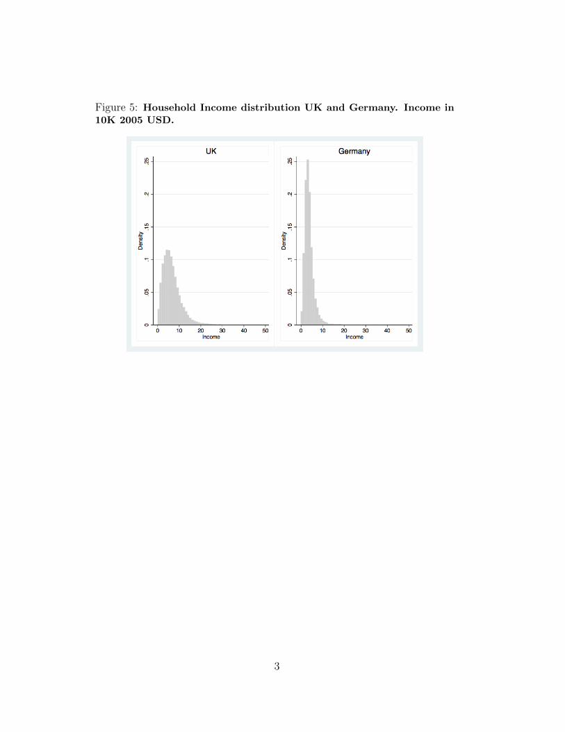
Household income In both SOEP and BSHP datasets the income has
been transformed in USD at 2005 constant prices, using the Consumer Price
Index (CPI) of World Bank-World Development indicators, data on income
are in 10K units. In figure 5 in the appendix we show histogram of Income
distribution for UK and Germany.
Control variables In almost all regressions, we control for demographic
variables as age and gender, marital status, number of children in the house-
hold, academic qualifications, number of visits to the doctor, to control for
7
the health status. We will also introduce dummies to control for region of
residence and labor force participation status like home caring, unemployed,
retired and so on. In some regression we also introduce labor environment
related controls, like worked hours, sector, socioeconomic status and firm
size.
3 Analysis
Figures 1 and 2 display the residuals Life Satisfaction – after controlling
for age, age2, gender and wave–, as a function of income for individuals in
different quintiles of score of each Personality trait, in UK and Germany
respectively (similar patterns would be displayed even if we consider the raw
Life Satisfaction data). In individuals with high Neuroticism score, the curve
is more concave and the peak is reached at levels of income lower than average
and for those with low score the relation seem to be always non decreasing
(like in the UK) or the decreasing part is very mild (like in Germany). No
other trait has such a clear effect on the relation we are analyzing: in none of
the other traits the distributions of the two extremes are both significantly
different from the distribution of the average.
The curves in figures 1 and 2 represent fractional polynomial interpola-
tion. The fractional polynomial is far more flexible of the conventional linear
and quadratic functions limited in their range of curve shapes, at the same
time they do not feature the undesirable aspect of the higher-order curves
that often fit badly at the extremes (Royston and Altman 1994), a problem
particularly serious for our data containing very high income levels. We will
discuss more on the reliability of the fractional polynomial fitting in section
5 where we will present evidence that the relationship between income and
life satisfaction is in general hump-shaped.
Figures 1 and 2 are based on data pooled across wave, in order to exploit
the longitudinal nature of our dataset by taking into account individuals’
8
heterogeneity and exclude the role of possible omitted variables, we estimate
a number of econometric models controlling for a large number of potentially
confounding factors. For computational reasons we need to assume a more
rigid functional form. A quadratic form seems in principle to approximate
well the data, but given its symmetry it would give excessive weight to the
high level of income. By excluding incomes larger than 800K USD per year
in UK (42 observations) and 700K USD in Germany (45 observations) a
quadratic regression of income over life satisfaction residuals generate an
interpolating curve with a peak at 231K for Germany and 276K for the UK,
similar to the peak reached in the dashed line curves in figures 1 and 2
respectively ( that we recall, it represents the interpolating lines using the
fractional polynomial fitting without income exclusions). In the appendix
we show that results are qualitatively robust with different incomes’ upper
bound.
Accordingly, we will estimate the following econometric model:
hit = β1yit + β2y2it + β′1θiyit + β′2θiy
2it + Γzit + Λθi + εi + ηt + eit (1)
where i represents the individual and t the year of the survey, hit is Life Sat-
isfaction , yit the household income. The individual fixed effect is described
as Λθi + εi, where
θi = (Ni, Ei, Ci, Ai, Oi,Mi) (2)
with N = Neuroticism,E = Extraversion, C = Conscientiousness, A =
Agreeableness,O = Openness,M = Male and εi is the individual specific
random effect. Moreover β′1θiyit + β′2θiy2it are the terms interacting each per-
sonality trait index with the income variables; vector, zit, consists of time
changing individual characteristics: age, age2, Marital state (a set of dum-
mies depending on whether the respondent is married, divorced, separated or
widowed), Education (a set of dummies measuring high school achievement,
vocational training or college degree); number of children in the household,
9
Region of residence (a set of dummies one for each region of residence of the
household), Health status (a set of dummies indicating intervals in terms of
number of visits to the doctor); Labor force participation (a set of dummies
depending on whether the individual is employed, house carer, unemployed,
retired); occupation types (a large set of dummies for socioeconomic status
(manager, employed, professional, white-collar, blue collar, farm-worker and
so on), worked hours per week and its squared term; ηt is a year (and wave)
fixed effect and eit is random noise.
In table 3, we report the OLS estimation the model 1,5 the estimation re-
sults confirms the pattern of figures 1 and 2 by showing that in both datasets
Neuroticism is the only trait to affect the relation between Income and Life
Satisfaction in a qualitatively similar way. In particular, from column 1
we note that in Germany, Neuroticism decreases the elasticity between in-
come and life satisfaction for income larger than about 120K USD, while
it decreases the elasticity for smaller incomes. From column 3, in the UK
Neuroticism decreases the elasticity for income larger than about 330K USD,
while it increases it otherwise.
A possible concern is that there is an error of measurement on the person-
ality traits due to difference in languages or reporting biases. We therefore
rescale each personality trait i of the individual j, Ti,j, according to the
formula
Ti,j =Ti,j −Min[PTQj]
Max[PTQj]−Min[PTQj](3)
where PTQj is the vector representing each single of the 15 reports of the
personality questionnaire for each individual j. In table 10 of the appendix
we present the results of the estimation of the model 1 with the adjusted
trait. They are qualitatively the same and quantitatively very similar to the
one in table 3.
Although in the range of age considered traits are stable, there is still a
significant small variation (for example in a regression of neuroticism with
5In the appendix, table 12 we report the result of the ordered probit estimations
10
age and age2 the R2 = 0.0027 in the SOEP and R2 = 0.0025 in the BHPS).
Therefore in table 11 of the appendix, we present the estimations of the
model 1 using the residuals of the traits after controlling for age and, to
control for the effect of gender differences in traits, we also introduced the
terms Male*Income and Male*Income2. Again the results are qualitatively
similar, Neuroticism is the only trait that in both datasets systematically
affect the elasticity between income and life satisfaction.
4 Happiness and Personality
The data we have seen suggest that Neuroticism affects systematically the
relation between Life Satisfaction and Income, increasing its elasticity for low
and medium income and decreasing it for high income levels. To provide a
possible explanation, we present a model based on the modern personality
traits theory; we then show that this model is able to produce an equation
similar to equation 1 as a reduced form and we will estimate this model using
an appropriate econometric estimator. In the model, behavior is explained
by traits that characterize an individual, rather than by optimization.
We use the convention that the coefficients are assumed to be positive.
The terms eit;uit; vit are error terms. The model has three equations. The
dependent observable variables are the household income yit and the life
satisfaction hit. The dependent latent variable is the desired income for any
individual i at time t is denoted by ait.
The Level of income depends on the desired income:
yit = α2 + β2ait + uit (4)
We assume that α2 > 0 and β2 ∈ (0, 1). The interpretation of the equation:
the aspiration to an income ait induces (through effort, persistence, and con-
fidence) a real level of income that is increasing in the aspiration level, but at
a rate smaller than 1. Individuals with low aspirations in average overshoot
11
by earning more. The linear form is for convenience: what is essential is that
the relationship is monotonic and has decreasing returns.
We summarize the argument in the following hypotheses: (i) higher mo-
tivation produces aspiration to higher income, and hence to higher realized
income; (ii) High aspirations are necessary to become rich, but the higher
they are, the more likely it is that they go unfulfilled. The effect of aspi-
ration on realized income however occurs at a decreasing rate. This is the
standard assumption of decreasing marginal returns. To illustrate it, con-
sider the search for a new occupation. An individual searching for a job may
set a reservation wage to be reached before he stops searching. The higher
the aspiration level the higher the wage found will be, everything else being
equal, although perhaps at a later date. Increasing aspiration may increase
realized income, however, only up to a point.
Given that we do not observe the desired income, ait, we are not able to
test the assumption made on equation 4. However, we consider the ques-
tion present in the SOEP dataset, “do success is important in job?”, coded
from Unimportant (1) to Very Important (4).6. The answers to this question
correlate positively and significantly with the traits implying motivations:
openness, conscientiousness and extraversion (and negatively with the oth-
ers). Therefore, it is natural to assume that Individuals who believe that suc-
cess on the job is important have high aspirations. Table 15 in the appendix
shows a concave relation between importance of success and the household
income in a regression with individual fixed effect. This is consistent with
our hypothesis of income with decreasing marginal return in aspirations.
The Life Satisfaction depends on the realized income and other variables:
6This question is present in the waves 1990, 1992, 1995, 2004, 2008 and it is inverselycoded.
Several predictions follow from our model. Higher income may be associ-
ated with higher cost of the gap between expectation and realization. This
cost is proportional to Neuroticism; hence higher Neuroticism implies higher
loss for high incomes, associated with higher gap. Once we control for the
effect of the interaction between Neuroticism and income, the residual effect
on Life Satisfaction of income should be positive. On the other hand, lower
income individuals may be associated with the real income to overshoot the
aspired income, for this reason highly neurotic individuals with lower income
might enjoy an increase of income even more than low neurotic individuals
7More precisely:
B =(1− β2) (β2γ1 − 2α2γ2)
β22
C = −2 (1− β2) γ2β22
D = λN −α22γ2β22
− α2γ1β2
F = − γ2β22
G =β2γ1 − 2α2γ2
β22
8Here
A2 = α2 + α0β2
B2 = β2η0
C2 = β2Γ0
D2 = β2Λ0,
16
because of the removed threat of not fulfilling aspirations.
In other words, from the estimation of the reduced form equation 9 we
expect that that both γ1 and γ2 are negative. The sign of the coefficient
of Niy2it must be negative if γ2 < 0. The sign of the coefficient of γ1 is
not identified but provided that γ2 < 0 a positive coefficient of Niyit, B,
might well be compatible with γ1 < 0, this happens especially if α2 is large,
i.e. individuals with low income (and low aspiration) overshoot more often.
Therefore the benefit of more income in terms of life satisfaction increases
more due to this extra-effect of overshooting on aspirations. Furthermore,
we will identify the direct effect of income on life satisfaction characterized
by parameters β1 and δ. We expect this direct effect being always positive
or at least non negative.
Motivation is likely to increase income; hence Openness, Conscientious-
ness and Extraversion (traits underlying motivation) should affect income
positively.9 Personality traits should also have direct effects (not necessarily
interacting with income) on Life Satisfaction, with Neuroticism reducing Life
Satisfaction and Extraversion increasing it.
We therefore test these predictions estimating the system represented by
equations 9 and 10. We show in section B of the appendix that the system
can be estimated by using a two or a three stage least square estimator.
The results presented in table 4–, where we used the year the traits have
been measured– are largely in line with our predictions. In the equation for
Life Satisfaction, the estimated coefficients of the interaction of Neuroticism
and income are negative and significant for the quadratic term in both sam-
ples. Once the effect of Neuroticism is taken into account, income has a linear
positive effect on life satisfaction on life satisfaction in the German dataset,
while in the UK data it appears non significant. The reason of this difference
is perhaps due to the fact that in Germany life satisfaction is measured in
9Boyce et al. (2010) succesfully test a related assumption that conscientiousness mat-ters for life satisfaction indirectly when interacted with unemployment
17
10 points scale, while in the UK is measured on a 7 points scale, so there is
more variability in the former.
The estimates for the Household Income equation in table 4 report the
effects of personality on income. Conscientiousness, Openness and Extraver-
sion increase income significantly, whereas Neuroticism decreases income.
The effects per year are noticeable: for example in the UK sample the size
is around 7K USD for Conscientiousness, 9K USD for Openness, −11.5K
USD for Neuroticism, and 8.6K USD for Extraversion. For comparison, the
effect of Male is 3.3K USD per year, hence the effects of some personality
traits are between two and four times larger than the gender gap. These
results confirm that personality traits are important for predicting life out-
comes, income in this case (see Roberts et al. (2007) Burks et al. (2009) for
other life outcomes). Consistently with the literature (Cohen et al. (2003),
Vitters and Nilsen (2002)), the direct effects of Neuroticism on Life Satis-
faction are negative, large and significant; those of Extraversion are positive
and significant.
As we argued above there is widespread agreement among psychologists
that traits are largely exogenous and stable, and this holds for the sample
we are considering (non students from 18 to 65 years). Still, we address the
possibility that traits are endogenous by using the entire panel of data. In
this way we are considering a span of 26 years of data for Germany and 12
years for the UK while the traits are relative to a single year. In table 5 we
present the estimation of the same equations as in table 4, but this time using
the entire panel of data available for the two countries, with a Two Stage
Least Square estimator (2SLS) with random effect. The results are largely
in line with the one in table 4: the interactions between Neuroticism and
income are positive and the ones with squared income are negative. Once
neuroticism is taken into account, the simple relation between income and
life satisfaction is increasing for Germany and non significant for the UK.
Our empirical test provides therefore a support of our theory based on the
18
gap between aspiration and income, explaining our above findings that Life
Satisfaction declines faster at higher income when Neuroticism is higher. Fur-
ther research will explore the merit of alternative explanations. A plausible
alternative hypothesis, always consistent with the notion of Neuroticism as
elasticity to punishment, is that higher income is also associated with higher
variance of the income; this higher income variance and the associated an-
ticipated anxiety might hurt the level of Life Satisfaction in individuals with
higher score in Neuroticism. In this explanation the effect of Neuroticism is
produced by the anticipation of future fluctuations in income, rather than
the comparison with past aspiration levels. This hypothesis is harder to test
with the data we are using, although we see it as complementary to the one
discussed here.
5 The hump-shaped Relation between income
and Life satisfaction
We showed that neuroticism is responsible of the decreasing elasticity in the
relation between income and life satisfaction, in figures 1 and 2 we note that
for level of Household Yearly Income larger than about 250K for Germany
and about 290K for UK this translate in a decreasing relation. Figure 3
shows the fractional polynomial fitting of the life satisfaction residuals after
controlling for age, gender and wave on Household Income (this corresponds
to the dashed lines of figures 1 and 2), with the 95 percent confidence level.
The number of observation with incomes larger than each bliss point is rea-
sonably large: there are 146 individuals and 213 total observations in the
German data and 264 individuals and 379 total observations in the UK data.
Note that In the BHPS data, the share of individuals with income above
290K 2005 USD is 0.3 percent in 2005 and in the same year the share of
individuals reporting an income above 210K is just above 1 percent. This
figure is very similar if we consider the minimum income reported by top 1
19
percent of individuals in the UK official statistics for the 2005 fiscal year.10
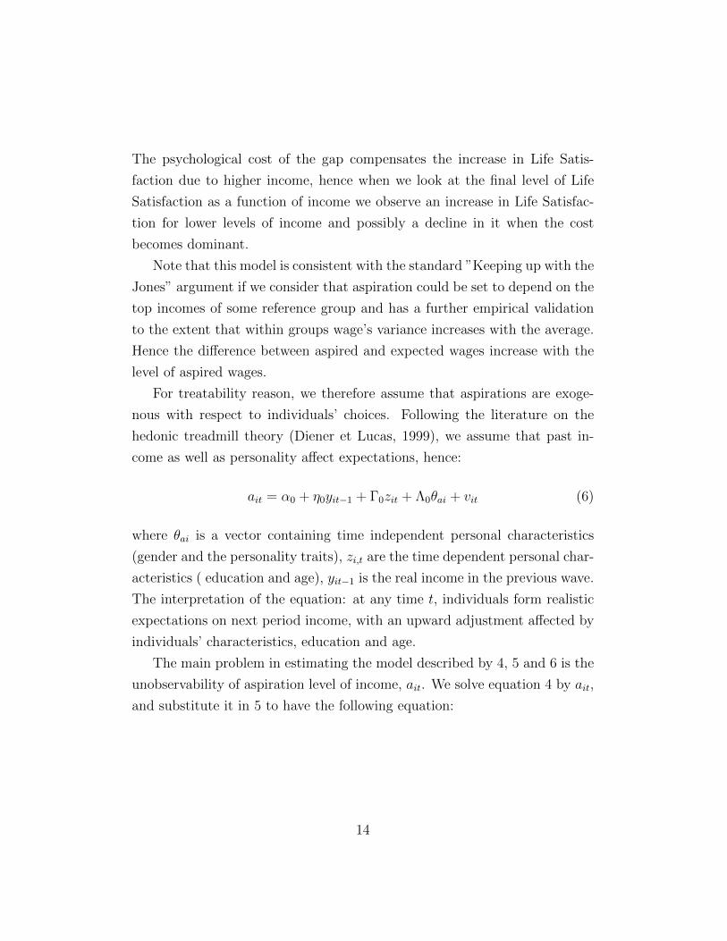
The analytical representation of the curves depicted in figure 3 is β0 −β1X
0.5 + β2X0.5logX for Germany; and : β0 − β1X0.5 + β2X for UK data,
where X represents a linear function of the income. We tested the effective-
ness of the fractional polynomial in predicting correctly the existence of a
bliss point using a Monte Carlo procedure to find that when we simulate a
logarithmic relation between income and life satisfaction, the best fractional
polynomial is a non decreasing function with a 99 percent confidence interval
(the outcomes of the simulations are available upon request).
Figure 4 displays the relationship between Average Life Satisfaction for
individuals within the same 1K income brackets and Household Income in
Germany and UK (a similar pattern would be displayed if we use the residuals
of Life Satisfaction after regressing it on age and gender, as we did in the
previous figures). We consider individuals between 18 and 65 years of age.
We note a statistically significant hum-shaped relation.
To exclude the role of omitted variables and controlling for individual
effects, we estimate a number of econometric models using the same controls
we used to estimate equation 1. We therefore run a series of regression
specifications based on the following general form:
hit = β1yit + β2y2it + Γzit + fi + ηt + eit (11)
where i represents the individual and t the year of the survey, hit is Life
Satisfaction , yit the household income, vector, zit, consists of time changing
individual characteristics, the same used in equation 1; fi is an unobserved
time invariant characteristics, like gender or personality trait. ηt is a year
(and wave) fixed effect and eit is random noise. In table 6 we estimate 11 using
an an OLS estimator with individual fixed effect, for Germany and UK.11 For
10To the best of our knowledge there are not similar readily available official statisticsfor Germany
11In the appendix, table 13, we report a similar estimation using an ordered probit
20
the reason already mentioned we exclude from the UK data observations with
an income larger than 800K per year and from the German data income larger
than 700K per year. Nevertheless in table 16 in the appendix we show how
results changes only quantitatively with different income upper thresholds.
The coefficient of the linear term is positive and significant and the
quadratic negative and significant. As we can see in column 1 for Germany
the turning point is about 264K, while in column 2 we note that for the UK
it is about 305K. The turning points are roughly similar to the ones in Figure
3. This implies that the quadratic interpolating lines of the regressions that
exclude individuals with income above 800K in the UK data and individuals
with income above 700K in the German data, are similar to the polynomial
line depicted in figure 3, which is calculated by using the whole set of data.
Always in table 6, it is instructive to compare column 2 and 3 for UK.
The turning point disappears in the UK data, when we introduce the marital
status: divorced and separated. Therefore the negative slope of the relation
seems to be linked to the household dynamics between partners at least in
UK. However, we note from table 3 that marital status does not affect the
interactions between income and neuroticism, suggesting that neuroticism
affect the interaction between income and life satisfaction through deterio-
ration in marital status (although this effect cannot be observed in German
data).
In table 7 we regress the individual life satisfaction against dummies indi-
cating 50K income brackets. It shows consistent results: in both datasets the
coefficient of the dummies indicating an income larger than 300K is smaller
than the one in the brackets [250K; 300K]. In the german data, in columns
1 and 2, the hypothesis that those coefficient are equal can be rejected at 5
percent confidence level, while in the UK data it is not possible to reject such
hypothesis.12 Table 7 therefore suggests an hump-shaped relation between
estimator and a logit estimator with individual fixed effect12The hypothesis that the dummies’ coefficient, indicating an income larger than 100K,
are equal in the UK data cannot be rejected, with the only exception of the the coefficient
21
income and life satisfaction similar to the one in figures 3 and 4 and in table
6.
Using the World Value Survey data, Figure 6 of the Appendix shows a
comparable pattern for US, the only country in the WVS for which an 11
income brackets scale is available. We see that Life Satisfaction distribution
in the last income group – the 11th income bracket for individuals with an
household income larger than 175K 2006 USD – is stochastically dominated,
with a p−value close to 5 percent, by the one in the 10th brackets.
The effect of household income on Life Satisfaction could be generated by
an increase of inequality within household. Clark (1996) shows that within
partners’ inequality has a negative impact on individual satisfaction. Con-
sidering table 8 we note that the squared income terms interacted with the
gender variable is non significant. Furthermore, in table 9, where the main
independent variable is individual labor income (rather than the households’
aggregate income) there is a similar hump-shaped relation between income
and life satisfaction. Both tables 8 and 9, seem to rule out inequality within
household as a possible explanation of the hump-shaped pattern.
Finally a word deserves the possible objection that the bliss point can be
determined by measurement errors. The fact that they are closely connected
to neuroticism excludes random mistakes in the data compilation. Given
that we observe a hump-shaped relation even when we control for individ-
uals fixed effect a possibility is that individuals lies in exaggerating their
income increase but do not lie in their life satisfaction report. According to
the existing literature in income measurement errors this is not a commonly
recorded bias. Studies comparing income reported in survey with external
source almost invariably conclude that in survey individuals tend to under-
report incomes (see More et al 2000 for a review of this studies). A study
based on the SOEP dataset argue that the typical behavior of individuals
who believe his income is inadequate is to refuse to respond (Schrapler 2002).
of [200K; 250K] larger than the coefficient [150K; 200K]
22
Finally, we note that the inflation of income for vanity is not a typical be-
havior for a neurotic individuals.
6 Conclusions
Neuroticism is responsible for slow increase (or even decline) of Life Satis-
faction with high income and its increase for lower incomes. Our hypothesis
suggests that the effect is due to the psychological cost of the gap between
aspiration and realized income, positive for lower incomes’ level and negative
for higher income levels. Motivation induces higher aspirations in income,
and on average also to higher incomes. This effect occurs however at a de-
creasing rate, and thus generates a gap between desired and realized income
which is negative and in absolute values higher for higher incomes, and this
in turn induces a decrease in Life Satisfaction. Neuroticism measures the
sensitivity to the gap, and in fact individuals with higher score in neuroti-
cism have a stronger decline of happiness with income, for high income and
a stronger increase for lower income when, the gap is positive.
This conclusion suggests a different interpretation of the well established
fact that life satisfaction increases slowly, or is completely flat at high lev-
els of income (Kanheman and Deaton 2010). This finding has been so far
interpreted with the argument that the marginal life satisfaction is decreas-
ing, just as utility. Our results suggest a stronger reason: the flatness of
happiness with income is the effect of opposite forces on Life Satisfaction:
a natural effect of increasing happiness with income, and a negative effect
induced by the gap between aspiration and realization. This second effect
becomes dominant for high incomes, but is likely to operate over a much
larger spectrum. If this is the case, then our results concern the life satis-
faction of a substantial fraction of the population, and not just the very rich
individuals.
Furthermore, our analysis shows that Life Satisfaction may be decreasing
23
in income for high levels of income. The finding is puzzling if one assumes that
people earn income as a mean to increase happiness. We saw the phenomenon
has an explanation when we bring personality traits into the analysis: they
explain the pattern of the relationship between happiness and income.
Table 1: Germany: SOEP dataset years 1984-2009, Main Variables
used in the regressions
Variable Mean Std. Dev. Min. Max. N
Life Satisfaction 5.078 1.158 0.636 7 330140
Income 3.853 2.47 0 151.554 314967
Age 41.777 12.841 18 65 331114
Male 0.491 0.5 0 1 331114
Neuroticism 0.501 0.2 0 1 223984
Extraversion 0.634 0.188 0 1 224018
Conscentiouseness 0.826 0.15 0 1 223260
Openness 0.577 0.2 0 1 223000
Agreeableness 0.739 0.162 0 1 223853
Labor Income 3.392 2.773 0.001 155.691 238754
Hours worked 28.693 20.279 0 80 310016
Table 2: UK: BHPS dataset years 1996-2008, Main Variables used
in the regressions
Variable Mean Std. Dev. Min. Max. N
Life Satisfaction 5.145 1.267 1 7 119367
Income 6.658 4.72 0 187.543 139308
Age 41.236 12.794 18 65 139308
Male 0.468 0.499 0 1 139307
Neuroticism 0.451 0.215 0 1 107713
Extraversion 0.584 0.192 0 1 107539
Conscientiouseness 0.725 0.174 0 1 107427
Continued on next page...
24
... table 2 continued
Variable Mean Std. Dev. Min. Max. N
Openness 0.581 0.195 0 1 107330
Agreeableness 0.741 0.163 0 1 107595
Hours worked 25.96 18.825 0 99 135418
Labor Income 2.56 1.627 0 105.518 89393
Figure 1: Life satisfaction, Household Income and Personality Traitsin UK. The five graphs show the fractional polynomial best fitting of theLife Satisfaction residuals with Income for the entire sample (dashed line),and the one related to the individuals belonging to the last quintile (lowestscore, dotted lines with confidence intervals) and to the first quintile (highestscore, solid lines with confidence intervals) in the traits distribution.
25
Figure 2: Life satisfaction, Household Income and Personality Traitsin Germany. See caption in figure 1.
Figure 3: Individuals Life satisfaction and Household Income. Frac-tional polynomial best of the Life Satisfaction residuals with Income.
26
Figure 4: Average Life satisfaction, Household Income. The verticalaxes report the average Life Satisfaction of all those individuals who arewithin the same interval of income of 1K width. The individuals with incomeexceeding 400K have been averaged together in the last 1K income bracket.The broken lines are the lowess estimate and polynomial fittings (almost nondistinguishable).
27
Table 3: Life Satisfaction Income and Personality Traits in UK andGermany. Panel Data with Individual Random Effects. Dependent variableis Life satisfaction, all regressions include control for Age, Age2, Gender,omitted from the table. Individuals who reported household income largerthat 700K USD and larger than 800K USD are excluded from respectivelyGerman and UK Data. (p-values in brackets, robust std errors)
Germany Germany UK UK UK1984-09 1984-09 1996-08 1996-08 1996-08
(0.0000) (0.0000) (0.0000) (0.0000) (0.0000)Wave effects Yes Yes Yes Yes YesRegion effects Yes Yes Yes Yes YesNumber of children Yes Yes Yes Yes YesMarital status Yes Yes Yes Yes YesEducation Yes Yes Yes Yes YesEmployment status Yes Yes Yes Yes YesOccupation type Yes Yes Yes Yes YesHealth Status Yes Yes Yes Yes YesWorked Hours Yes Yes Yes Yes NoWorked Hours2 Yes Yes Yes Yes No
r2N 180985 180985 90703 90623 92927
28
Table 4: Life Satisfaction, Household Income and Personality Traitsin a 3SLS structural model. Dependent variable is Life Satisfaction,Income is in 10K USD, traits are normalized between 0 and 1 (p-values inbrackets, robust std errors).
Germany Germany UK UK2005 2005 2005 2005b/p b/p b/p b/p
Life SatisfactionIncome 0.032 0.050*** –0.024 0.002
(0.000) (0.000) (0.000) (0.000)Income at t−1 0.412*** 0.411*** 0.612*** 0.619***
(0.000) (0.000) (0.000) (0.000)
N 13738 13738 9979 9979
29
Table 5: Life Satisfaction Income and Personality Traits, structural2SLS model using the entire panel of Germany and UK data. De-pendent variable is Life Satisfaction, Income is in 10K USD, traits are nor-malized between 0 and 1. Estimates of the structural model using a 2SLSestimator with individual random effects. Individuals who reported house-hold income larger that 700K USD and larger than 800K USD are excludedfrom respectively German and UK Data. (p-values in brackets, robust stderrors).
Table 6: Life Satisfaction and Household Income in Germany andUK Panel OLS with individual fixed effect for the German and UK data.Dependent variable is individual Life Satisfaction. Income is the HouseholdIncome in 10K 2005 USD. Controls for Employment status includes dum-mies for student, retired, unemployed, house-caring. Controls for occupationtype are 43 dummies for German and 38 for UK data and includes sectors,socioeconomic groups and number of co-workers, health status is measuredin terms of visits to the doctor. Individuals who reported household incomelarger that 700K USD and larger than 800K USD are excluded from respec-tively German and UK Data. (p-values in brackets, robust std errors).
(0.0000)Wave effects Yes Yes YesRegion effects Yes Yes YesNumber of children Yes Yes YesEducation Yes Yes YesEmployment status Yes Yes YesMarital status Yes No NoOccupation type Yes Yes YesHealth Status Yes Yes Yes
r2 0.043 0.021 0.023N 260838 114304 115134
31
Table 7: Life Satisfaction and Household Income in Germany andUK Dependent variable is individual Life Satisfaction. Income is the House-hold Income in 10K 2005 USD (p-values in brackets).
Germany Germany UK UKOrd. Probit OLS Panel fe Ord. Probit OLS Panel fe
b/p b/p b/p b/pmainIncome in [50K;100K] 0.2078*** 0.0669*** 0.1753*** 0.0443***
(0.0000) (0.0000) (0.0000) (0.0000)Income in [100K;150K] 0.4286*** 0.1513*** 0.2386*** 0.0479***
(0.0000) (0.0000) (0.0000) (0.0002)Income in [150K;200K] 0.4630*** 0.1404*** 0.2495*** 0.0321
(0.0000) (0.0011) (0.0000) (0.1491)Income in [200K;250K] 0.6160*** 0.1742** 0.3565*** 0.0784**
(0.0000) (0.0187) (0.0000) (0.0312)Income in [250K;300K] 0.6112*** 0.2701** 0.3711*** 0.0781
(0.0000) (0.0000) (0.3919) (0.1015)Wave effects Yes Yes Yes YesRegion effects Yes Yes Yes YesNumber of children Yes Yes Yes YesEducation Yes Yes Yes YesEmployment status Yes Yes Yes YesMarital status Yes Yes No NoOccupation type Yes Yes Yes YesHealth Status Yes Yes Yes Yes
r2 0.040 0.021N 273457 273457 114335 114335
32
Table 8: Life Satisfaction, Income and Gender. Panel Data with In-dividual Fixed Effects. Dependent variable is Life satisfaction, it includescontrol for age, age2. Individuals who reported household income larger that700K USD and larger than 800K USD are excluded from respectively Germanand UK Data. (p-values in brackets, robust std errors),
Germany UK1984-09 1996-08
b/p b/pIncome 0.0425*** 0.0075***
(0.0000) (0.0067)Income2 –0.0008*** –0.0001**
(0.0000) (0.0304)Male*Income 0.0119** 0.0003
(0.0133) (0.9439)Male*Income2 –0.0002 0.0000
(0.3060) (0.6755)Age –0.0117 –0.0491***
(0.7115) (0.0006)Age2 0.0003*** 0.0004***
(0.0000) (0.0000)Worked hours 0.0087*** 0.0016
(0.0000) (0.1825)Worked hours2 –0.0001*** –0.0000
(0.0000) (0.1257)Wave effects Yes YesRegion effects Yes YesNumber of children Yes YesEducation Yes YesEmployment status Yes YesMarital status Yes NoOccupation type Yes YesHealth Status Yes Yes
r2 0.043 0.021N 260838 114304
33
Table 9: Life Satisfaction and Individual Labor Income with differentincome boundary. Panel Data with Individual Fixed Effects. Life satisfactionis the dependent variable, income is in 10K USD. Apart the regression withUK data and all observations, the peaks are always significantly smaller thanthe income upper bound ( p-value < 0.01 ). p-values in brackets, robust stderrors.
Germany Germany UK UKIncome< 600K All Income< 700K All
b/p b/p b/p b/pLabor Income 0.0597*** 0.0417*** 0.0338*** 0.0257***
(2003), Emotional Style and Susceptibility to the Common Cold. Psy-
chosomatic Medicine, 65, 652-657.
[16] Costa, Paul T. and McCrae, Robert R., (1980), Influence of extraversion
and neuroticism on subjective well-being: Happy and unhappy people,
Journal of Personality and Social Psychology, 38, 668-678.
[17] Deaton, A. (2008), Income, Health and Well-Being around the World:
Evidence from the Gallup World Poll. Journal of Economic Perspectives
22, 53-72.
36
[18] DeYoung, C. G., Peterson, J. B., Sguin, J. R., Pihl, R. O., and Tremblay,
R. E. (2008), Externalizing behavior and the higher-order factors of the
Big Five, Journal of Abnormal Psychology, 117, 947-953.
[19] DeYoung C. G. , Gray J. R. (2010), Personality Neuroscience: Explain-
ing Individual Differences in Affect, Behavior, and Cognition, in P. J.
Corr and G. Matthews (Eds.), The Cambridge handbook of personality
psychology, New York: Cambridge University Press.
[20] DeYoung, C. G., Hirsh, J. B., Shane, M. S., Papademetris, X., Rajee-
van, N., and Gray, J. R. (2010). Testing predictions from personality
neuroscience: Brain structure and the Big Five. Psychological Science,
21, 820828.
[21] Diener, E., and R.E. Lucas, (1999). Personality and subjective well-
being. In D. Kahneman, E. Diener, and N. Schwarz (Eds.), Well-being:
The foundations of a hedonic psychology (pp. 213229). New York: Rus-
sell Sage Foundation.
[22] Diener, Ed, Diener, M. and Diener C. (1995), Factors Predicting the
Subjective Well-Being of Nations. Journal of Personality and Social Psy-
chology, 69, 851-864.
[23] Duesenberry, James S. 1949. Income, Saving, and the Theory of Con-
sumer Behavior. Cambridge and London: Harvard University Press
[24] Easterlin, R. A. (1974), Does Economic Growth Improve the Human
Lot? Some Empirical Evidence. In Nations and Households in Economic
Growth: Essays in Honor of Moses Abramovitz, ed. R. David and M.
Reder. New York: Academic Press, 89-125.
[25] Easterlin, R. A. (1995), Will Raising the Incomes of All Increase the
Happiness of All? Journal of Economic Behavior and Organization, 27,
35-47.
37
[26] Easterlin, R. A. (2005), Feeding the Illusion of Growth and Happiness:
A Reply to Hagerty and Veenhoven. Social Indicators Research, 74, 429-
443.
[27] Ferrer-i-Carbonell, A., and Frijters. P. (2004), How Important Is
Methodology for the Estimates of the Determinants of Happiness? Eco-
nomic Journal, 114: 641-659.
[28] Gosling, S. D., Rentfrow, P. J., and Swann, W. B., (2003), A very brief
measure of the Big-Five personality domains. Journal of Research in
Personality, 37, 504-528.
[29] Inglehart, R. (1990), Cultural Shift in Advanced Industrial Society.
Princeton: Princeton University Press.
[30] John, O. P., Naumann, L. P., and Soto, C. J. (2008), Paradigm shift
to the integrative Big Five trait taxonomy: History: measurement, and
conceptual issue. In O. P. John, R. W. Robins, and L. A. Pervin (Eds),
Handbook of personality: Theory and research, 114-158, New York,
Guilford Press.
[31] John, O. P., and Srivastava, S. (1999), The Big Five trait taxonomy:
History, measurement, and theoretical perspectives. In L. A. Pervin and
O. P. John (Eds.), Handbook of personality: Theory and research (2nd
ed., pp. 102-138). New York: Guilford.
[32] Kahneman, D., Krueger, A.B., Schkade, D., Schwarz, N., and Stone,
A.A. (2006). Would you be happier if you were rich? A focusing illusion.
Science, 312, 1908-1910.
[33] Kahneman, D. and Deaton, A., (2010), High income improves evalua-
tion of life but not emotional well-being, Proceedings of the National
Academy of Sciences, 107, 16489-16493.
[34] Kimball, Miles S., and Robert J. Willis. 2006. Happiness and Utility.
University of Michigan mimeo.
38
[35] Layard, R., Mayraz, G. and Nickell, S., 2008. The marginal utility of
income, Journal of Public Economics, vol. 92(8-9), 1846-1857, August.
[36] Loehlin. J. C. (1992). Genes and environment in personality develop-
ment. Newbury Park, CA: Sage.
[37] McCrae, R.R. and Costa, P.T., 1990. Personality in Adulthood. New
York: The Guildford Press.
[38] McCrae, R. R., and Costa, P. T. (1997), Conceptions and correlates of
Openness to Experience. In R. Hogan, J. Johnson, and S. Briggs (Eds.),
Handbook of personality psychology. Boston, Academic Press.
[39] McCrae, R. R., and Costa, P. T., Jr. (1999), A five factor theory of per-
sonality. In L. A. Pervin and O. P. John (Eds), Handbook of personality:
Theory and research (102-138), New York, Guilford Press.
[40] Moore, J. C., Stinson, L. L., and Edward J. Welniak, J. 2000. Income
Measurement Error in Surveys: A Review. Journal of Official Statistics,
16(4):331362.
[41] Ozer, D. J. and Benet-Martinez, V. (2006), Personality and the pre-
diction of consequential Outcomes, Annual Review of Psychology, 57,
201-221.
[42] Paulhus, D. L., Lysy, D. C., and Yik, M. (1998), Self-report measures of
intelligence: Are they useful as proxy IQ tests? Journal of Personality,
66, 525-554.
[43] Reimann, R., Angleitner, A., and Strelau, J. (1997). Genetic and envi-
ronmental influences on personality: A study of twins reared together
using the self- and peer report NEO-FFI scales. Journal of Personality,
65, 449-476.
[44] Roberts B. W., Nathan R. Kuncel, Rebecca Shiner, Avshalom Caspi
and Lewis R. Goldberg, (2007), The Power of Personality. The Com-
parative Validity of Personality Traits, Socioeconomic Status, and Cog-
39
nitive Ability for Predicting Important Life Outcomes, Perspectives on
Psychological science, 2, 313-345.
[45] Royston, P., and D. G. Altman,1994 Regression using fractional poly-
nomials of continuous covariates: Parsimonious parametric modelling.
Applied Statistics 43: 429467
[46] Schrapler J.P., 2002, Respondent Behavior in Panel Studies - A Case
Study for Income-Nonresponse by means of the German Socio-Economic
Panel (GSOEP), DIW dp 299
[47] Stutzer, A. ,2004 The Role of Income Aspirations in Individual Happi-
ness. Journal of Economic Behavior and Organization 54(1), pp. 89-109.
[48] Spoont, M. R. (1992). Modulatory role of serotonin in neural informa-
tion processing: Implications for human psychopathology. Psychological
Bulletin, 112, 330-350.
[49] Vitterso, J. and Nilsen, F., (2002), The Conceptual and Relational
Structure of Subjective Well-Being, Neuroticism, and Extraversion:
Once Again, Neuroticism Is the Important Predictor of Happiness, So-
cial Indicators Research, 1, 89-118.
40
For Online Publication
Appendices
A The ”Big Five” in the SOEP and BHPS
datasets
I see myself as someone who:
1. (A) Is sometimes rude to others (reverse-scored).
2. (C) Does a thorough job.
3. (E) Is talkative.
4. (N) Worries a lot.
5. (O) Is original, comes up with new ideas.
6. (A) Has a forgiving nature.
7. (C) Tends to be lazy (reverse-scored).
8. (E) Is outgoing, sociable.
9. (N) Gets nervous easily.
10. (O) Values artistic, aesthetic experiences.
11. (A) Is considerate and kind to almost everyone.
12. (C) Does things efficiently.
13. (E) Is reserved (reverse-scored).
14. (N) Is relaxed, handles stress well (reverse-scored).
15. (O) Has an active imagination.
1
B Estimating the Structural Model
Now we determine the correct estimator for the model represented by equa-
tions 9 and 10. The error term of the latter, εyit = β2vit + uit, poses no
problem, given that both 2SLS and 3SLS are non biased estimator when
errors are cross-correlated between equations.
Considering now the 9, this can be rewritten as:
hit = α1 + β1yit + δy2it − γ(
1− β2β2
)2
Niy2it − (Cuit +B)Niyit+
−Ni
(FE(u2) +Guit +D
)+ FNi
(u2it − E(u2)
)+ Γ1zit + λEEi + eit
(12)
Its error term can be written as:
εhit = −GNiuit − CNiyituit + eit (13)
Given 4, yit and uit are correlated by construction. Substituting 10 in 13,
we obtain:
εhit =−GNiuit − CNi(A2 +B2yit−1 + C2zit+
D2θai + β2vit + uit)uit + FNi
(u2it − E(u2)
)+ eit
(14)
from where we note that
E(εhit)− CNiE(u2) = 0. (15)
Therefore, we define εhit = εhit + CNiE(u2) and we rewrite 12, as:
hit = α1 + β1yit + δy2it − γ(
1− β2β2
)2
Niy2it −BNiyit+
−Ni
((F + C)E(u2) +D
)+ Γ1zit + λEEi + εhit,
(16)
whose errors satisfy the conditional mean condition: E(εhit|Ni, Ei, yit, zit) = 0.
2
Figure 5: Household Income distribution UK and Germany. Income in10K 2005 USD.
3
Figure 6: USA: Happiness distributions in different income brackets.The broken lines refer always to the richer of each pair. (Income expressed in 11brackets). CDF of Life Satisfaction is in terms of residuals after removing theeffects of age age2 gender, year. In last panel, comparing groups with incomein bracket 10 (income between 150K and 174K USD in the 2006 wave) and inbrackets 11 (income >175K USD in the 2006 wave), the Kolmogorov-Smirnov testrejects the hypothesis that life satisfaction for poorer contains smaller values thanfor richer with a p−value = 0.937, while the opposite hypothesis hypothesis thatlife satisfaction for poorer contains larger values than for richer cannot be rejectedat 10 percent confidence level, with a p−value = 0.063
4
Table 10: Life Satisfaction Income and Individually Adjusted Per-sonality Traits in UK and Germany. Panel Data with Individual Ran-dom Effects. Dependent variable is Life satisfaction, all regressions includecontrol for Age, Age2, Gender, omitted from the table. Individuals who re-ported household income larger that 700K USD and larger than 800K USDare excluded from respectively German and UK Data. (p-values in brackets,robust std errors)
Germany Germany UK UK UK1984-09 1984-09 1996-08 1996-08 1996-08
(0.0000) (0.0000) (0.0000) (0.0000) (0.0000)Wave effects Yes Yes Yes Yes YesRegion effects Yes Yes Yes Yes YesNumber of children Yes Yes Yes Yes YesMarital status Yes Yes Yes Yes YesEducation Yes Yes Yes Yes YesEmployment status Yes Yes Yes Yes YesOccupation type Yes Yes Yes Yes YesHealth Status Yes Yes Yes Yes YesWorked Hours Yes Yes Yes Yes NoWorked Hours2 Yes Yes Yes Yes No
r2N 180907 180907 90623 90623 92846
5
Table 11: Life Satisfaction Income and Residuals of PersonalityTraits in UK and Germany. Panel Data with Individual Random Ef-fects. Dependent variable is Life satisfaction, all regressions include controlfor Age, Age2, Gender, omitted from the table. Individuals who reportedhousehold income larger that 700K USD and larger than 800K USD are ex-cluded from respectively German and UK Data. (p-values in brackets, robuststd errors)
Germany Germany UK UK1984-09 1984-09 1996-08 1996-08
Income 0.0605*** 0.0588*** 0.0099*** 0.0106***(0.0000) (0.0000) (0.0001) (0.0000)
Wave effects Yes Yes No NoRegion effects Yes Yes No NoNumber of children Yes Yes Yes YesMarital status Yes Yes Yes YesEducation Yes Yes Yes YesEmployment status Yes Yes No NoOccupation type Yes Yes No NoHealth Status Yes Yes No NoWorked Hours Yes Yes No NoWorked Hours2 Yes Yes No No
N 180985 180985 93725 93725
6
Table 12: Life Satisfaction, Household Income and Traits, OrderedProbit estimators. In the Ordered probit models the dependent variableis individual Life Satisfaction. Income is the household income in 10K 2005.Individuals who reported household income larger that 700K USD and largerthan 800K USD are excluded from respectively German and UK Data. (p-value < 0.001). p-values in brackets, robust std errors. USD
Germany Germany UK UK1984-09 1984-09 1996-08 1996-08
(0.0000) (0.0000) (0.0000) (0.0000)Wave effects Yes Yes Yes YesRegion effects Yes Yes Yes YesNumber of children Yes Yes Yes YesMarital status Yes Yes Yes YesEducation Yes Yes Yes YesEmployment status Yes Yes Yes YesOccupation type Yes Yes Yes YesHealth Status Yes Yes Yes YesWorked Hours Yes Yes Yes NoWorked Hours2 Yes Yes Yes No
r2N 180985 180985 90651 92874
7
Table 13: Life Satisfaction and household, Ordered Probit and Logitestimators. In the Ordered probit models the dependent variable is indi-vidual Life Satisfaction, the individual random effect is included. In the logitmodels the dependent variables are expressed in terms of deviation from thepersonal life satisfaction intertemporal average, so that the dependent vari-ables take the value 1 when the report is above or equal to each individual’saverage and 0 otherwise (see Ferrer-i-Carbonell and Frijters 2004). Income isthe household income in 10K 2005. Individuals who reported household in-come larger that 700K USD and larger than 800K USD are excluded from re-spectively German and UK Data. The peaks are always significantly smallerthan the income upper bound (p-value < 0.001). p-values in brackets, robuststd errors. USD
Germany Germany UK UKOrd.Probit Logit Ord.Probit Logit
(0.000) (0.000)Wave effects Yes No Yes YesRegion effects Yes Yes Yes YesNumber of children Yes Yes Yes YesMarital status Yes Yes Yes NoEducation Yes Yes Yes YesEmployment status Yes Yes Yes YesOccupation type Yes No Yes YesHealth Status Yes No Yes YesWorked Hours Yes Yes Yes YesWorked Hours2 Yes Yes Yes Yes
N 180985 262419 90651 101967
8
Table 14: Life Satisfaction, traits and household Income: differentincome boundary. Panel Data with Individual Random Effects. Life sat-isfaction is the dependent variable, all regressions include control for age,age2, gender, worked hours, worked hours2; income is in 10K USD. p-valuesin brackets, robust std errors.
Gearmany Geamany UK UKAll income< 500K All income< 500K
(0.0000) (0.0000) (0.0000) (0.0000)Wave effects Yes Yes Yes YesRegion effects Yes Yes Yes YesNumber of children Yes Yes Yes YesMarital status Yes Yes Yes YesEducation Yes Yes Yes YesEmployment status Yes Yes Yes YesOccupation type Yes Yes Yes YesHealth Status Yes Yes Yes Yes
r2N 181004 180974 92954 92885
9
Table 15: Income and Job Motivation in Germany. Panel Data withIndividual Fixed Effects. Dependent variable is Household Income, (p-valuesin brackets, robust std errors)
Germany Germany Germany GermanyIncome Income Income Log(Income)
b/p b/p b/p b/pSuccess Important 0.2211*** 0.1914*** 0.1759***
Table 16: Life Satisfaction and household Income: different incomeboundary. Panel Data with Individual Fixed Effects. Life satisfaction isthe dependent variable, income is in 10K USD.( p-value < 0.01 ). p-valuesin brackets, robust std errors.
Germany Germany UK UKAll income< 500K All income< 500K