Research Division Federal Reserve Bank of St. Louis Working Paper Series Lifetime Labor Supply and Human Capital Investment Rodolfo E. Manuelli Ananth Seshadri And Yongseok Shin Working Paper 2012-004A http://research.stlouisfed.org/wp/2012/2012-004.pdf February 2012 FEDERAL RESERVE BANK OF ST. LOUIS Research Division P.O. Box 442 St. Louis, MO 63166 ______________________________________________________________________________________ The views expressed are those of the individual authors and do not necessarily reflect official positions of the Federal Reserve Bank of St. Louis, the Federal Reserve System, or the Board of Governors. Federal Reserve Bank of St. Louis Working Papers are preliminary materials circulated to stimulate discussion and critical comment. References in publications to Federal Reserve Bank of St. Louis Working Papers (other than an acknowledgment that the writer has had access to unpublished material) should be cleared with the author or authors.
Transcript
Research Division Federal Reserve Bank of St. Louis Working Paper Series
Lifetime Labor Supply and Human Capital Investment
Rodolfo E. Manuelli Ananth Seshadri
And Yongseok Shin
Working Paper 2012-004A http://research.stlouisfed.org/wp/2012/2012-004.pdf
February 2012
FEDERAL RESERVE BANK OF ST. LOUIS Research Division
The views expressed are those of the individual authors and do not necessarily reflect official positions of the Federal Reserve Bank of St. Louis, the Federal Reserve System, or the Board of Governors.
Federal Reserve Bank of St. Louis Working Papers are preliminary materials circulated to stimulate discussion and critical comment. References in publications to Federal Reserve Bank of St. Louis Working Papers (other than an acknowledgment that the writer has had access to unpublished material) should be cleared with the author or authors.
Lifetime Labor Supply and Human Capital Investment
Rodolfo E. Manuelli∗ Ananth Seshadri† Yongseok Shin‡
January 24, 2012
Abstract
We develop a model of retirement and human capital investment to study the effectsof tax and retirement policies. Workers choose the supply of raw labor (career length)and also the human capital embodied in their labor. Our model explains a significantfraction of the US-Europe difference in schooling and retirement. The model predictsthat reforms of the European retirement policies modeled after the US can deliver15–35 percent gains in per-worker output in the long run. Increased human capitalinvestment in and out of school accounts for most of the gains, with relatively smallchanges in career length.
JEL classification: E24; J24; J26Keywords: Human capital; Labor supply; Retirement
∗Washington University in St. Louis and Federal Reserve Bank of St. Louis†University of Wisconsin-Madison‡Washington University in St. Louis and Federal Reserve Bank of St. Louis
1 Introduction
Micro and macro estimates of how aggregate labor supply responds to policies and shocks
display significant variance. Micro estimates of this elasticity—when aggregate labor supply
is measured by total number of hours—are close to zero, while macro studies obtain much
larger numbers. Recently, researchers have developed models that are consistent with both
micro and macro estimates—for example, Imai and Keane (2004).
We take a different tack. We view the economically-meaningful notion of labor input—
which we call effective labor—as consisting of two components: a quantity component (or raw
labor) measured by career length, on which the micro-macro elasticity debate is centered,
and a quality component that depends on education and other forms of human capital
investment. From this perspective, to assess the economic effects of policies and shocks, it
is necessary to understand how they affect human capital investment decisions as well as
participation and retirement choices. We find that even the macro elasticity substantially
underestimates the economic impact of tax and retirement policies.
The key elements of our model are labor-leisure choices at the extensive margin, human
capital investment in and out of school, and retirement policies that introduce rigidities
in workers’ labor supply decisions.1 We assume that individuals choose years of schooling,
human capital investment in school, and on-the-job training, as well as the supply of raw la-
bor. In our model, leisure, which gives extra utility, is indivisible (i.e., labor supply decisions
are at the extensive margin only). Retirement is defined as the endogenously back-loaded
leisure consumption. Finally, we model retirement benefits as a non-linear function of life-
time income and retirement age that encapsulates the most salient features of real-world
policies.
Our analysis shows that, for both qualitative and quantitative reasons, it is important
to endogenize schooling, age-earnings profile, and retirement choices. By contrast, most
existing work endogenizes only one of them, while either taking the others as exogenously
given or abstracting from them altogether.
To be more specific, we use the Ben-Porath (1967) technology for human capital invest-
ment, augmented with retirement decisions. Unlike in learning-by-doing models (i.e., models
with costless human capital accumulation), which are more widely used, human capital in-
vestment in our model is not hard-wired into decisions on raw labor supply. Consequently,
we can capture and analyze the interactions between human capital investment and the sup-
ply of raw labor. In addition, our model allows us to consider schooling decisions as well as
on-the-job human capital investment within a single framework.
1The first two are what Keane and Rogerson (2010) consider to be important for useful models of laborsupply, and the third is emphasized by Ljungqvist and Sargent (2011) in their review article.
2
We use the model to explore, both theoretically and quantitatively, the impact of changes
in taxes, retirement policies, and other shocks. In our analysis, we emphasize how a given
change prompts individuals to respond along several margins simultaneously. For example,
higher taxes discourage them from acquiring human capital both in and out of school, and,
at the same time, induce earlier retirement.
Theoretically, we first show that a reduction in the degree of redistribution in taxes and
transfers increases workers’ retirement age and human capital investment.
We then explore the effects of three kinds of unanticipated shocks. First, we show that
negative wealth shocks raise the retirement age. Second, we find that a permanent decrease in
the rental rate of human capital induces older workers to retire earlier but has an ambiguous
impact on younger workers’ retirement, which depends on the relative strength of income and
substitution effects. In addition, for young workers, such a shock flattens their age-earnings
profile: upon impact, their effective labor supply increases as they allocate more time to
market work and less to human capital investment, but over time their human capital and
effective labor supply are lower than what they would have been in the absence of the shock.
Finally, we study the effect of an unanticipated drop in the stock of human capital (e.g., a
loss associated with reallocation in the presence of firm or sector-specific human capital).
We show that older workers supply less effective labor and retire earlier. Again, its impact
on the retirement of younger workers is ambiguous because of the interplay between income
and substitution effects.
For our quantitative exercises, we calibrate the model to the data on output per worker,
taxes, and retirement policies for the United States and several European countries. We
obtain two main results.
First, the impact of taxes and retirement policies on effective labor supply is substan-
tial, with the policies affecting both the quantity and the quality components of effective
labor. These policies explain a large fraction of the gap in retirement age between European
countries and the US, and almost all of their difference in schooling.
Second, a policy reform that institutes the US-style retirement tax/benefit regime has
large effects on output per worker in the European countries that we study, with long-run
increases of 15 to 35 percent. In all cases we find that the response of career length—the
extensive margin emphasized by the more recent literature—is relatively small. The main
reason is that changes in retirement age are often accompanied by changes in schooling in the
same direction, pushing career length in opposite directions. In our model, the large long-run
economic impact materializes primarily through human capital investment decisions, both
in school and on the job. In this sense, we reconcile the view of Prescott (2006), Ljungqvist
and Sargent (2007), and Prescott, Rogerson, and Wallenius (2009), who emphasize the large
3
impact of tax policies on aggregate output, with the seemingly opposing view of Ljungqvist
and Sargent (2010), who emphasize the rigidities built into nonemployment benefits that
result in the typical worker being at a corner and, hence, his choice of career length not
responding significantly to policy changes.2
Our analysis shows that the retirement and human capital investment decisions reinforce
each other, and that the full impact of tax and retirement policies cannot be captured without
a model that allows individuals to adjust both the quantity and the quality components of
their effective labor. For example, most studies on the fiscal sustainability of retirement
policies abstract from the endogenous response of workers’ human capital to policy changes
(Gruber and Wise, 2007). In light of our results, we conjecture that these studies may
grossly underestimate the full economic impact of the proposed reform of tax and retirement
policies.
2 Model
We adapt the model of human capital accumulation of Ben-Porath (1967) to allow for en-
dogenous labor supply at the extensive margin. We develop a model that complements the
standard continuous-time life cycle—which is essential to understand retirement decisions—
with a dynastic preference structure that guarantees a tractable characterization of the
long-run equilibrium. Individuals choose years of schooling and human capital investment
while in school. When in the labor force, they decide how to allocate their time between
market work and investment in human capital. Leisure, which gives extra utility out of
goods consumption, is indivisible, and retirement in the model is endogenous back-loading
of leisure. Finally, we model retirement benefits as a non-linear function of lifetime income
and retirement age.
Life Cycle The individual life span is deterministic and runs from age 0 to T . From age 0
to I, an individual is attached to his parent, who makes decisions for him. He then becomes
independent at age I. At age B, he gives birth to ef children, who remain attached to him
until they turn age I. We assume I ≤ B.
Choices From age a = 6 through T , an individual is endowed with one unit of time at any
given point. Time endowment can be spent on leisure, ℓ(a), investment in human capital,
2Note that in a learning-by-doing model, human capital investment is hard-wired into raw labor supply(e.g., career length) decisions. In other words, if there is no change in raw labor supply, there cannot be anychange in human capital. In our model, even if a worker is at a corner in terms of raw labor supply, he canstill change his human capital investment decisions both in and out of school, thereby changing his supplyof effective labor.
4
n(a), and market work, 1 − n(a) − ℓ(a). Leisure is a binary variable: ℓ(a) ∈ {0, 1}.3 Both
n(a) and 1−n(a)−ℓ(a) must belong to the closed interval [0, 1]. The individual also chooses
consumption, c(a), and goods input to human capital production, x(a).
In addition, he makes decisions for his children while they are attached to him. He
chooses goods inputs for early childhood human capital production, xE , when they turn
6. Between their age 6 and I, with subscript k denoting variables for a child, he chooses
their time allocation and goods inputs in human capital accumulation: {nk(a), ℓk(a), xk(a)}.
When children are between ages 0 and I, he chooses their consumption, ck(a). Finally, when
they reach age I and become independent, he gives each child a bequest of qk.
Preferences An independent adult orders allocations in terms of the utility derived from
his own consumption and leisure, and also all his descendants’ utility. The parent’s inter-
generational altruism may be imperfect as in Barro and Becker (1989). His preferences are
represented by
∫ T
I
e−ρ(a−I)U(c(a), ℓ(a))da +
∞∑
t=1
e−(α0−α1f)t
∫ T
0
e−ρ(a+Bt−I)U(ct(a), ℓt(a))da.
The first term is the utility from his own consumption and leisure, where ρ is the subjective
discount rate. The second term is the utility he derives from his descendants, with t indexing
generations. Note that α0 and α1 control the degree of intergenerational altruism. The case
with α0 = 0 and α1 = 1 corresponds to the standard dynastic preferences, while a positive
α0 or an α1 less than 1 imply imperfect altruism.
We use the following specification for the flow utility:
U(c, ℓ) =(c(1 + ζℓ))1−θ
1 − θ,
with parameters ζ and θ satisfying:
(c(1 + ζ))1−θ
1 − θ>
c1−θ
1 − θ.
This specification can accommodate both the view that consumption drops at retirement
because of the substitutability between home and market goods (French, 2005; Laitner and
3Since leisure is binary, measured hours of work, which equals one minus leisure in the post-schoolingperiod, is also binary. The assumption of indivisible labor supply has a long tradition in both macro andmicroeonomics. Two examples are the lotteries of Rogerson (1988) and the retirement model of Rust andPhelan (1997). Fixed costs associated with working can justify this indivisibility, especially at retirement.French and Jones (2011) estimate the daily fixed time cost to be about 3.26 hours at age 60. Rogersonand Wallenius (2010) show that the fixed time cost needs to be more than the equivalent of a half-time jobin order to create the downward discontinuity in hours at retirement, with an intertemporal elasticity ofsubstitution of labor supply lower than or equal to 0.5.
5
Silverman, 2008) and the view that, in order to supply labor to the market, it is necessary
to purchase some goods such as transportation and meals outside home (Aguiar and Hurst,
2009).4
Human Capital Production We adopt the Ben-Porath (1967) formulation of the human
capital production technology, modifying it to include an early childhood period.
h(a) = zh(n(a)h(a))γ1x(a)γ2 − δhh(a), a ∈ [6, T ] (1)
h(6) = hBxνE (2)
Equation (1) is the standard human capital production developed by Ben-Porath, with h(a)
denoting the human capital stock at age a and δh the depreciation rate. The technology
to produce a child’s human capital at age 6, h(6), is given by (2), where hB is the stock
of human capital at birth and xE is goods input. This specification captures the idea that
nutrition and health care are important determinants of early levels of human capital, and
that these inputs are essentially market goods. We assume that γ1, γ2, and ν are all between
0 and 1.
Schooling, On-the-Job Training, and Retirement Human capital produced at age a
can be used until age T , subject to depreciation, and human capital has no value once an
individual reaches age T . This is why, as we show later, he will choose to front-load his
human capital production, and n(a) weakly decreases with age. In fact, there can be an
age interval [6, 6 + s] in which individuals are at a corner, using all his time allotment on
human capital production, i.e., n(a) = 1. We interpret this interval as the schooling period,
with s standing for years of schooling. Note that we use the same human capital production
function (1) both in and out of school.
At the same time, individuals in our model will choose to back-load their leisure, with
ℓ(a) = 1 for a ∈ (R, T ] and ℓ(a) = 0 for a ∈ [6, R], with 6 < R ≤ T . We interpret R as
the retirement age. As we show in the appendix, back-loaded leisure is the consequence of
human capital depreciation and the equilibrium interest rate being greater than or equal to
subjective discount rate.5
Figure 1 shows a typical life-cycle choices of n(a) and ℓ(a). On the left panel, an individual
uses all his time endowment for human capital production, i.e., n(a) = 1, from age 6 to 6+s.
4Consider a utility function u(cl, cw, ℓ). In this formulation cl denotes consumption not related to supply-ing labor, and cw denotes consumption necessary to supply labor. Given that total consumption expendituresare given by cl + cw = c, the indirect utility function is u(c, ℓ) = maxcl
u(cl, c − cl, ℓ). In particular, with
u(cl, cw, ℓ) =
(cφ(1−ℓ)+ℓ
l c(1−φ)(1−ℓ)w
φφ(1 − φ)1−φ
)1−θ
1
1 − θ,
6
Schooling (s)
a
n
1
06 6+s R T
1 − n(a) ℓ(a)s
Retirement (R)
a
ℓ
1
06 R T
Figure 1: Schooling and Retirement Decisions
This is the schooling period, which lasts s years. While in the labor force, i.e., between age
6 + s and R, he supplies 1 − n(a) of his time to the labor market, and uses n(a) of his time
producing human capital. The latter can be labeled as on-the-job training.
Whereas in our model n(a) is the time spent on human capital production during the
working period and not on market work, one can think of an alternative interpretation. Imag-
ine an environment where jobs are different in terms of learning contents/opportunities. In
the labor market equilibrium of this alternative economy, jobs with more learning possibili-
ties will pay lower rental rate of human capital, and a worker’s choice of n(a) is equivalent
to a choice over different jobs. This is essentially the theory of occupation mobility in Rosen
(1972).
The right panel shows the leisure choice through the life cycle. Only after he reaches
age R, which will be chosen endogenously, he will spend all his time enjoying leisure, i.e.,
ℓ(a) = 1, until age T .
Effective Labor Supply We are primarily interested in the economic impact of taxes and
retirement policies. As such, it is important that we make a distinction between pure quantity
measures of raw labor supply (e.g., hours or years worked) and labor services measured in
efficiency units. In our framework, the measure of raw labor supply is career length or the
number of years worked, since our leisure vs. labor supply decision is only at the extensive
margin.6 The career length is R− (6 + s), with the worker entering the labor market at age
the indirect utility function u(c, ℓ) coincides with our specification with 1 + ζ = (φφ(1 − φ)1−φ)−1.5Age-dependent retirement benefits can also induce the back-loading of leisure, but they are not necessary
in our model.6Our analysis complements the work of Prescott et al. (2009), who also emphasize the distinction between
raw labor supply and labor services. Their analysis focuses on the intensive margin (hours worked).
7
6 + s and exiting to retire at age R.
In the model, labor services in terms of efficiency units are measured by the amount of
human capital supplied for market work. To be more specific, we define he(a) ≡ (1− n(a)−
ℓ(a))h(a) as the effective labor supply. The amount of effective labor an individual supplies
to the market is zero when he is in school—n(a) = 1 and ℓ(a) = 0—or in retirement—
ℓ(a) = 1 and n(a) = 0. During his working career, it depends on his human capital stock,
h(a), and the fraction used for market work, 1 − n(a).
Taxes and Transfers The government taxes labor income at rate τ . In our formulation,
τ ≡ τI + τS, where τS is the social security tax rate. Capital income is taxed at rate τK .
With the income tax revenue, the government pays for retirement benefits, other transfers
not tied to retirement (denoted with u), and government consumption. We denote with
b(a, R) the retirement benefit at age a for an individual whose chosen retirement age is R.
Retirement benefits will depend on a retiree’s past earnings, and we will fully specify them
in Section 3.1.
Net Labor Income We describe the life-cycle profile of an individual’s labor income net
of taxes and goods input to human capital production. In particular, take an individual with
s ≥ 0 years of schooling and retirement age R. Let w be the rental rate of human capital
and p be the tax-adjusted price of goods input to human capital production. The unit price
of early-childhood goods input is pE. His net (of taxes and goods input) income at age a is
as follows.
y(a, R) =
0 0 ≤ a < 6−pExE a = 6−(1 − τ)px(a) 6 < a ≤ 6 + s(1 − τ)[wh(a)(1 − n(a)) − px(a)] 6 + s < a ≤ Rb(a, R) R < a ≤ T
Until age 6, individuals are not endowed with time and there is no human capital pro-
duction or market work. We summarize the expenditures on early childhood human capital
investment as a lump-sum payment at age 6, pExE . From age 6 to 6 + s, net income is
the negative of the market goods expenses for schooling, −(1 − τ)px(a), as the individual
supplies no market labor. The active labor market period (i.e., his career) runs from age
6+ s to R. During this period, the net income is (1− τ)[wh(a)(1−n(a))− px(a)]. We allow
for the possibility that a fraction ξ of goods input to human capital is tax-deductible. Thus,
given the income tax rate τ , p is given by p = (1− τξ)/(1− τ). Note that the tax treatment
8
of goods input is assumed to be the same whether the individual is in school or working.
Finally, b(a, R) is the retirement benefit, which we assume is not taxed.
Individual’s Problem We assume that an individual can freely borrow and lend at the
after-tax real interest rate r ≡ (1 − τK)r, although he is not allowed to die in debt. The
budget constraint is given by
∫ T
I
e−r(a−I)c(a)da + ef
∫ I
0
e−r(a+B−I)ck(a)da + efe−rBqk
≤
∫ T
I
e−r(a−I)y(a, R)da + ef
∫ I
6
e−r(a+B−I)yk(a, Rk)da + q + u, (3)
where q is the bequest that the individual starts his independent life with, and u is the non-
retirement transfer from the government. The variables with subscript k are his children’s.
Note that the parent not only pays for his children’s consumption and goods input but also
receives their labor income—if any—until they become independent.
We denote the maximized value of an independent individual at age I who starts with h
units of human capital, bequest q, and non-retirement transfer from the government u by:
where the maximization is over {c(a), x(a), ℓ(a), n(a)}Ta=I , {ck(a)}I
a=0, {xk(a), ℓk(a), nk(a)}Ia=6,
xE , and qk, and is subject to the budget constraint (3) and the human capital production
technology in (1) and (2).
3 Theoretical Analysis
We first show that the individual’s problem can be transformed into an income maximization
problem. We then analyze how retirement decisions are made. In Section 3.2, we characterize
how an individual’s human capital investment and retirement decisions respond to policy
changes and unexpected shocks.
3.1 Solving Individual’s Problem
Given our preference specification and the assumption of perfect financial markets in par-
ticular, we can transform the individual’s problem into a version of income maximization
problem.
9
Before we begin, we clarify one aspect of the model: intergenerational linkage. For a
child, his parent makes decisions for him until he turns I. However, there is no discrepancy
between the choices his parent makes and what he would have chosen himself, even though the
intergenerational altruism is not perfect. To obtain this result with our dynastic preferences,
bequests must not be restricted. A heuristic argument establishing this equivalence is as
follows. Suppose that the parent does not choose investment in human capital to maximize
the present value of his children’s lifetime income. In this case, the parent could increase
the utility of each child by adopting the income-maximizing human capital investment and
adjusting the bequest to exactly offset the cost differential. The overall cost to the parent is
the same, but his children are—and hence he is, because of his (imperfect) altruism—now
made better off.
To solve the individual’s problem, one also needs to take into account retirement benefits
b(a, R), which typically depend on the labor income history. Let W (R) be the maximized
present value of net income between age 0 and R, for a worker who retires at age R. That
is,
W (R) = max
∫ R
0
e−r(a−I)y(a, R)da, (4)
where the maximization is over {x(a), n(a)}Ra=6 and xE , subject to the human capital pro-
duction in (1) and (2). This problem, for a given R, is solved in the appendix. We assume
that the retirement benefits are affine in W (R), during the eligible retirement period, so that
the individual’s optimal time and goods allocation is the same whether he maximizes the
present value of his net labor income between 0 and R or between 0 and T . This property
allows us to solve the problem in two steps, as shown below. The retirement benefits at age
a are specified as follows.
b(a, W (R); Rn) =
{0 a ≤ max{R, Rn}bm + byW (R) a > max{R, Rn}
Here, bm is a constant and byW (R) is the variable component of retirement benefits. In
addition, Rn is the normal retirement age set by law. Those who retire before Rn will have
to wait until they turn Rn to collect benefits. On the other hand, those who retire past Rn
forfeit the benefits between Rn and R.7
7Admittedly, our specification of retirement benefits is overly simplistic. However, it still captures themain features of actual programs. In particular, the assumption of the completely forgone benefits whileworking for those who work past the normal retirement age is an accurate description of the US socialsecurity system between 1950 and 1972. After 1972, a delayed retirement credit was reintroduced, but it isonly with rules that recently came into effect that the compensation became close to actuarially fair (Schulz,2001). This assumption is also consistent with the retirement benefit systems in many European countries
10
Let y∗(a, R) be the net labor income at age a that constitutes the maximized present
value of lifetime net labor income in (4). For later use, it is convenient to develop a notation
for partial sums of net labor income given R. Let
W (a1, a2, R) =
∫ a2
a1
e−r(a−I)y∗(a, R)da
be the properly discounted value of the net labor income between age a1 and a2. It follows
that W (0, R, R) = W (R).
We proceed in two steps. The first is to simplify and solve the individual’s problem for a
given retirement age R. This way, we obtain an indirect value function in R. In the second
step, we solve for the retirement age that maximizes the indirect value function.
Step 1: Nested Problem Given Retirement Age For a given retirement age R, which
we will solve for in the second step, we derive the optimal consumption decisions. Optimal
consumption must satisfy:
c(a) = c(I)e(r−ρ)(a−I)/θ, a ∈ [I, R], (5)
c(a) = c(I)e(r−ρ)(a−I)/θ(1 + ζ)1/θ−1, a ∈ (R, T ], (6)
where c(I) is the consumption at age I. To make consumption drop at retirement, lima↑R c(a) >
c(R), as is observed in the data, we assume θ > 1. The attached children’s consumption
must satisfy:
ck(a) = c(I)e(r−ρ)(a+B−I)−α0−(1−α1)f
θ , a ∈ [0, I). (7)
We further simplify the problem by looking at the sum of the utility that directly accrues
to the parent between his age I and T and the utility derived from his attached children.
Simple calculations using the consumption Euler equations (5), (6), and (7) turn this sum
into the right-hand side of (8):
∫ T
I
e−ρ(a−I)U(c(a), ℓ(a))da
︸ ︷︷ ︸direct utility for parent
+ e−α0+α1f
∫ I
0
e−ρ(a+B−I)U(ck(a), ℓk(a))da
︸ ︷︷ ︸utility from attached children
=c(I)1−θ
1 − θG(I, R),
(8)
(Gruber and Wise, 1999). In addition, the assumption that the benefits are a function of the present valueof net earnings but not the entire earnings history is a reasonable approximation to real-world programs.For example, the US social security benefits are determined by the average of a worker’s highest 35 years ofearnings.
11
where:
G(I, R) ≡ eυ(r)I[(∆(R) − ∆(I)) + (1 + ζ)
1−θθ (∆(T ) − ∆(R))
]+ eυ(r)I+f−rB−µ/θ∆(I)
(9)
∆(x) ≡
∫ x
0
e−υ(r)ada =1 − e−υ(r)x
υ(r)(10)
υ(r) ≡ρ − (1 − θ)r
θ> 0 (11)
µ ≡ α0 + (1 − α1)f + ρB − rB. (12)
The µ term captures the difference between the current interest rate r and the effective
discount rate for the utility of different generations (α0 + (1 − α1)f)/B + ρ.
The consumption expenditures for the parent, inclusive of the consumption of the at-
tached children, similarly simplify into the right-hand side using (5), (6), and (7):
∫ T
I
e−r(a−I)c(a)da
︸ ︷︷ ︸consumption of parent
+ ef
∫ I
0
e−r(a+B−I)ck(a)da
︸ ︷︷ ︸consumption of attached children
= c(I)G(I, R).
With this notation, the maximized utility of a parent of generation t at age I is, for a
Since GR(I, R) > 0, condition (15) implies that the marginal benefit of working exceeds
the marginal monetary cost at the equilibrium retirement age—if they were equal, the con-
dition would be WR(Rt) = 0. The reason is obvious. The opportunity cost of work is the
additional utility associated with leisure, which is captured by the right-hand side. In other
words, condition (15) equates the marginal benefit of additional work (i.e., additional net
income) with the forgone utility from leisure converted into units of income. Note that,
if Rt > Rn, the forgone retirement benefits are subtracted from the marginal benefit of
additional work, as shown in (16).
3.2 Properties of the Solution
In this section we demonstrate some properties of the solution to the individual problem.
In particular, we study the response of effective labor supply to changes in the economic
environment. To derive results in this section, we assume that the rental rate of human
capital w and the interest rate r are held constant.
We restrict our attention to the implications of the model when µ = 0, which corresponds
to the steady state.8 To see this, consider the case in which the interest rate exceeds the
8The definition of µ is in equation (12).
13
generational discount rate, i.e., µ < 0. One consequence is that consumption increases from
generation to generation, shifting the right-hand side of (15) upward over t. The second-
order condition implies that the retirement age, Rt, must decrease over generations indexed
by t.9 Intuitively, this is driven by income effects: Earlier retirement allows individuals to
enjoy more leisure. The case with µ > 0 can be worked out in a straightforward manner.
In the steady state (µ = 0), from the budget constraint (13), we obtain
c(I)G(I, R) = W (I, T, R) + ef−rBW (0, I, R) + (1 − ef−rB)q + u. (18)
Now, the relevant first-order condition for the choice of retirement age is, except at the
policy-induced kink:
WR(R)
W (I, T, R) + ef−rBW (0, I, R) + (1 − ef−rB)q + u=
θ
θ − 1
GR(I, R)
G(I, R), (19)
where we have replaced c(I) using (18).
3.2.1 Long-Run Responses
In this section, we consider the long-run effects of permanent changes in tax and retirement
policies. These are steady-state comparisons. The short-run transition effects are explored
in Section 3.2.2.
Effect of Changes in Retirement Benefits The above first-order condition (19) can
be used to study how the level and the redistributive nature of the retirement system affect
the retirement age. Consider an increase in the generosity of the retirement benefits as given
by an increase in the constant portion bm, with all else held constant. Through a standard
income effect, this policy change will lower the equilibrium retirement age. To see this, note
that the positive income effect associated with an increase in bm raises the denominator
of the left-hand side of (19). Moreover, depending on whether the worker retires after Rn
or before, WR(R) either decreases or stays the same as bm increases—see equations (16)
and (17). Thus, the left-hand side of equation (19) goes down while the right-hand side
remains the same, resulting in a decrease in the retirement age. Recall that the left-hand
side intersects the right-hand side from above, according to the second-order condition.
To isolate the impact of the redistributive nature of the retirement benefits, we consider
a joint change in bm and by that keeps the benefit level constant at the initial retirement
age R∗. More specifically, let the benefit level be b = bm + byW (R∗). The new b′m and b′ysatisfy b′m + b′yW (R∗) = b at the initial retirement age R∗. It follows that an increase in by
9This model predicts that there is a downward trend in retirement age when interest rates exceed theirlong-run values, which happens during the transition to the steady state.
14
accompanied by a decrease in bm to maintain b shifts the numerator of the left-hand side of
equation (19) upward. Its denominator will change, but it will be the same as before at R∗
by construction. Hence we know for sure that the left-hand side is now higher than before
at R∗. The right-hand side is unchanged. As a result, the retirement age rises.
R∗∗
R∗
Age
LHS of (19)
RHS of (19)
58 59 60 61 62 63 64 65 66 67
Figure 2: Retirement Decision Responding to Changes in bm and by
Figure 2 depicts this exercise. Initially, the left-hand side (solid gray line) of condition
(19) and the right-hand side (solid black line) cross at R∗, which is the optimal retirement
age. Given the changes in bm and by, the left-hand side moves up (dashed line), while the
right-hand side remains the same. The new optimal retirement age is at the new intersection,
denoted by R∗∗.
The intuition is straightforward. Returns to continued work increase as the system re-
duces the pure tax-and-redistribute component of the retirement benefits, resulting in later
retirement.
Now that the worker will retire at an older age, he will in turn increase his human capital
investment: As the time horizon over which human capital can be utilized lengthens, the
returns to human capital investment become higher. He will go to school for longer, and will
invest more in his human capital on the job as well.10
We conclude that it is not only the level of benefits but also their redistributive nature
that influences retirement and human capital investment decisions.
Effect of Changes in Tax Rates To better understand how the model works, and to build
an intuition that is relevant to the US-Europe comparison, we consider the following change
in taxes and transfers: We increase the tax rate τ and then commensurately increase the
non-retirement transfer u such that the denominator of the left-hand side of (19) evaluated
10Because of the way we set up the problem, the nested problem for a given retirement age is not affectedby the changes in bm and by considered here. As a consequence, human capital investment decisions wouldhave not changed, if the changes in bm and by somehow failed to affect the retirement age at all.
15
at R∗ is left unchanged. That is, the change in tax revenue is rebated lump-sum to the
consumer to control for the income effect channel at R∗.
Unlike the changes in retirement benefits we consider above, this tax-transfer change will
affect the individual human capital investment even when the retirement age is held constant.
Of course, this tax-transfer change will have an impact on the retirement age itself, and the
response of the retirement age will generate further responses in terms of human capital
investment.
First, we will go through the effect of this increase in tax rate τ for a fixed retirement
age. One immediate implication is that the goods input to human capital production is now
more expensive relative to the after-tax return to human capital. This is true as long as the
goods input is not fully deductible, i.e., ξ < 1.11 As a result, there will be less investment in
human capital. For one, the individual will choose less schooling, and he will use less goods
input for human capital production while in school. Likewise, he will reduce his investment
in human capital on the job. In summary, a higher tax rate, unless the goods input to human
capital production is fully tax-deductible, will reduce the amount of human capital a worker
acquires and, in turn, the lifetime supply of effective labor, even when the retirement age is
held constant.
Next, we explore the effect of this tax-transfer change on the retirement age. We revisit
the first-order condition (19). Note that the right-hand side is not affected. The numerator
of the left-hand side goes down, because (i) the tax rate is now higher and (ii) for a given R,
the worker now accumulates less human capital for the reason explained above. Thus, if we
compensate the worker with a higher transfer u such that the denominator of the left-hand
side of (19) evaluated at R∗ is unchanged, then we see that the retirement age goes down
unambiguously, together with the left-hand side of (19).12
Finally, now that the worker will retire earlier, he will further reduce his human capital
investment. This is an important interaction between retirement—i.e., a decision on the
career length—and the human capital investment decision. Note that the decrease in the
pure quantity measure of raw labor supply (career length) will underestimate the decrease
in labor services adjusted for human capital (effective labor). In our quantitative analysis in
Section 4.3, we find that the magnitude of this downward bias can be substantial.
3.2.2 Short-Run Responses
We now analyze the short-run response of a worker’s effective labor supply to three different
kinds of unanticipated shocks: a one-time drop in the value of accumulated non-human
11If ξ = 1, then we have p = 1, which means the relative price is not affected by tax rates.12The higher u for this purpose must compensate not only for the higher taxes but also for the lower
income due to lower levels of human capital.
16
wealth, a one-time drop in the stock of human capital, and a permanent decrease in the
rental rate of human capital.
To simplify the discussion, we assume that such shocks hit a worker of age a′ > I + B—
that is, his children have already left the household—so that he does not adjust bequests, and
his response captures standard life-cycle effects.13 In addition, for simplicity, we consider the
case in which the worker chooses R∗ < Rn in the absence of shocks, and the new retirement
age remains in this region.14
Shock to Non-Human Wealth The relevant version of (19) at age a′ for a worker whose
where A(a′) is the value of financial wealth accumulated up until age a′. As before, the
second-order condition requires that the left-hand side of (20) crosses the right-hand side
from above.
Now, consider the effect of an unanticipated (one-time) drop in the value of financial
wealth A(a′) the worker has accumulated so far. This shock decreases the denominator of
the left-hand side of (20), but WR(a′, T, R) is not affected. The left-hand side shifts up
and the right-hand side stays the same, increasing the retirement age—i.e., ∂R/∂A < 0.
Note that this shock only has a negative income effect, and leaves other dimensions—e.g.,
returns to work—unchanged. The worker chooses to consume less leisure, which necessitates
a delayed retirement.
Shock to Human Capital Next, we consider the effect of an unanticipated (one-time)
partial destruction of human capital at age a′. This could be interpreted as, for example, an
unanticipated reallocation of workers across sectors or firms when human capital is at least
partly sector or firm-specific.
The effect of this one-time shock on effective labor supply diminishes over time. To be
precise, for a fixed retirement age R, the effect of an exogenous change in h(a′), is given by,
from equations (32) and (33) in the appendix,
∂he(a)
∂h(a′)= e−δh(a−a′), a′ ≤ a < R,
13The results are qualitatively similar for ages under I + B, but the expressions are algebraically morecumbersome and the income effects must include the adjustment of bequests.
14If this is not the case, again, the qualitative results remain similar but the algebra needs to be adjusted.
17
where he(a) = (1 − n(a))h(a). That is, the younger the worker is when he is hit by this
negative shock, the smaller is the long-run impact on effective labor supply, for a given
retirement age. The intuition is clear: a one-time shock to the stock of human capital does
not alter the returns to human capital (i.e., the rental rate of human capital w) in the future.
Since younger workers have a longer horizon, they accumulate more human capital than older
workers.
Unlike in the previous case of the shock to non-human wealth, there is a substitution effect
in addition to a negative income effect. While the returns to human capital are not affected,
the shock reduces the returns to the worker’s time, as one unit of his time translates now
into less human capital supplied to the market or used for human capital production. The
income and substitution effects push the retirement age in opposite directions. A sufficient
condition for the substitution effect to dominate, and hence, for the worker to retire earlier
than originally planned is
r + δh
e(r+δh)(R∗−a′) − 1≥
θ
θ − 1
GR(a′, R∗)
G(a′, R∗).
It is easy to check that this condition is more likely to be satisfied for older workers (i.e.,
a′ closer to R∗). For an older worker, only a small fraction of his working life is in the
post-shock period, and hence the labor income generated after the shock accounts for only
a small fraction of his lifetime income. Thus, the income effect for him is much smaller than
his younger counterpart’s.
Permanent Wage Shock Finally, we ask what is the effect of an unanticipated permanent
decrease in the rental rate of human capital w for a worker whose age is a′. From equation
(33) in the appendix, for a fixed retirement age R,
∂he(a)
∂w=
γ2
1 − γ
Ch
w
(w
p
) γ21−γ1−γ2
π(a′, a), a > a′,
where he(a) is the supply of effective labor and
π(a′, a) ≡ (r + δh)
∫ a
a′
e−δh(a−u)m(u)γ1+γ2
1−γ1−γ2 du − γ1m(a)1
1−γ1−γ2
m(a) ≡ 1 − e−(r+δh)(R−a)
Ch ≡
(zh
r + δh
γγ1
1 γγ2
2
) 11−γ1−γ2
.
The sign of the impact on effective labor depends on the sign of π(a′, a). Let us first fix
R and a′ < R. Simple calculations show that for each a′ there exists ϕ(a′) ∈ (a′, R) such
18
that
π(a′, a)
< 0 if a′ ≤ a < ϕ(a′)= 0 if a = ϕ(a′)> 0 if ϕ(a′) < a ≤ R
This result shows that, immediately following a permanent decrease in the rental rate
of human capital, effective labor supply increases. The size of the increase depends on the
worker’s age: Young workers increase their effective labor supply more than old workers.
Over time, the effect on the effective labor supply of a change in the rental rate reverses
itself. For a given age a′ at the time of the shock, there exists another age, ϕ(a′) > a′, such
that the post-shock effective labor supply at that age coincides with what the effective labor
supply at that age would have been in the absence of the shock. Eventually, for a > ϕ(a′),
the post-shock effective supply of labor, he(a), drops below what it would have been without
the shock.
The intuition is as follows. When faced with a permanent decrease in the return to human
capital, our worker chooses to reduce investment in human capital. In the short run, this
results in more human capital supplied to the market as he changes his allocation of time
away from human capital production—i.e., a decrease in n(a). However, the lower levels of
investment in human capital push the stock of human capital below what it would have been
without the shock, eventually bringing down effective labor supply.
The response of earnings mirrors that of effective labor. For a fixed retirement age, the
adjustment in human capital investment implies that a drop in the human capital rental rate
flattens the age-earnings profile.
What is the impact on the retirement age? In general, it is not possible to determine
the effect on retirement because both the income and the substitution effects are at play.
A lower w reduces the marginal benefit of working, WR(a′, T, R), but the negative income
effect reduces the denominator in the left-hand side of (20), pushing the retirement age in
opposite directions. It is possible to show that for a′ close to R∗—i.e., for older workers—the
magnitude of the income effect is arbitrarily small, again because the post-shock working
period is only a small fraction of their overall working life. Thus, for older workers, the model
predicts that a decrease in w results in earlier retirement. The effect on the retirement plan
of younger workers is ambiguous.
To summarize, we find that the impact of unanticipated shocks on retirement depends
on the standard tension between income and substitution effects as well as on the specifics
of the determinants of the age-earnings profile. Unlike in most other models of lifetime
labor supply, the age-earnings profile in our model is endogenously determined and is not
independent of the nature of shocks.
19
4 Quantitative Analysis
In Section 4.1, we close the model by specifying the goods production side of the economy
and the government budget constraint. For our quantitative analysis, the preference and
technology parameters are calibrated to the relevant data for the US in Section 4.2.
Section 4.3 begins by asking whether differences in tax and retirement policies across
countries can explain their differences in schooling and retirement behavior. We then consider
three sets of exercises. First, we impose the retirement policies of the US onto selected
European countries. Second, we study the impact on the US economy of various policy and
demographic changes. Finally, we ask whether our model can explain the historical labor
market outcomes in the US circa 1900. In all the exercises, we focus on the impact of taxes
and retirement policies on schooling, retirement, and overall effective labor supply along the
life cycle.
4.1 Closing the Model
To define the steady-state equilibrium, we develop notations for the age distribution in the
population. Let η = f/B be the population growth rate. With the population size at any
give point in time normalized to one, the density for age a is
φ(a) =ηe−ηa
1 − e−ηT.
We assume that the aggregate goods production function is Cobb-Douglas in physical
capital and effective labor, with aggregate productivity z: zF (K, H). Let κ be the ratio of
physical capital to effective labor, and δk be the depreciation rate of physical capital. Using
this notation, output per worker is
y = zF (κ, 1)
∫ R
6+she(a)φ(a)da
∫ R
6+sφ(a)da
, (21)
and output per capita is
y = zF (κ, 1)
∫ R
6+s
he(a)φ(a)da. (22)
The steady-state equilibrium requires that the goods market clear:
We assume competitive factor markets, and hence firms equate the marginal product to
factor prices:
r = (1 − τK)(zFK(κ, 1) − δk), (24)
w = zFH(κ, 1), (25)
where FK and FH respectively denote the marginal product of physical and human capital.
We assume that the retirement benefits are fully financed by the social security taxes on
labor income at all times. That is, the revenues collected from labor income at rate τS are
equal to retirement benefit payments:
∫ T
max{R,Rn}
[bm + byW (R)]φ(a)da = τS
∫ R
6
[whe(a) − ξx(a)] φ(a)da,
where we take into account the partial tax deductibility of goods input to human capital
production. Furthermore, we assume that the government runs a balanced budget in terms
of non-retirement revenues and expenditures:
g + φ(I)u = τI
∫ R
6
[whe(a) − ξx(a)]φ(a)da + τK(zFK(κ, 1) − δk)κ
∫ R
6+s
he(a)φ(a)da,
where the left-hand side is the non-retirement expenditures and the right-hand side is the
sum of non-retirement labor income tax revenue and capital income tax revenue.
The definition of a steady-state competitive equilibrium is standard, and is omitted here.
4.2 Calibration
Certain parameters are standard in the macro literature. The interest rate is set at r = 0.04
and the depreciation rate is set at δk = 0.09. The income share of (physical) capital is set at
0.33. The parameters governing the altruism function, α0 = 0.24 and α1 = 0.35, are taken
from Manuelli and Seshadri (2009) who use observations on intergenerational transfers and
the endogenously-chosen fertility rate in a similar model to calibrate these parameters. In
the steady state (µ = 0), these parameters together with the discount rate (ρ = 0.027) and
the population growth rate (η = 0.01) pin down the real interest rate r = 0.04. For the
individual life cycle, we use T = 78, I = 23, and B = 25.
We use age-wage profiles to pin down the parameters that govern human capital produc-
tion. Little information is available on the fraction of job training expenditures that are not
reflected in wages, but there are many reasons why earnings ought not to be equated with
wh(1 − n) − x. First, some training is off the job and directly paid for by workers. Second,
firms typically obtain a tax break on the expenditures incurred on training. Consequently,
21
the government (and indirectly, workers through higher taxes) pays for the training, and this
component is not reflected in wages. Third, some of the training may be firm-specific, in
which case the employer is likely to bear the cost of the training, since the employer benefits
more than does the worker through such training. Finally, there is probably some smoothing
of wage receipts in the data and, consequently, the worker’s marginal productivity profile
could be steeper than his wage profile. For all these reasons, we equate measured earnings
in the model with wh(1 − n) − 0.5x. Because our model only has the extensive margin for
raw labor supply, age-wage profiles and age-earnings profiles in the model are the same.
Our theory implies that it is only the ratio h1−γB /(z1−υ
h wγ2−υ(1−γ1)) that matters for the
moments of interest. Consequently, we can choose w (which is determined by z, the produc-
tivity in the goods production function) and hB arbitrarily, and then calibrate zh to match
a desired moment. The calibrated value of zh is common to all countries. In other words, we
do not assume any cross-country difference in an individual’s ability to learn. This leaves us
with seven parameters: δh, zh, γ1, γ2, ν, ζ , and θ.
Since the moments are block-separable, as in Section 3.1, we proceed in two steps. First,
for a given retirement age, we calibrate the parameters δh, zh, γ1, γ2, and ν so as to match
the following five moments.15
1. The ratio of wage rate at age 64 to wage rate at age 55: 0.75 (French, 2005).
2. The ratio of earnings at age 50 to earnings at age 25: 2.5 (authors’ calculations using
NLSY 79).
3. Years of schooling for males aged 30-to-64 in the US as of 2005: 12.65 (Barro and Lee,
2010).
4. Schooling expenditures (primary and secondary) relative to GDP: 4.2% (UNESCO
Institute for Statistics).
5. Pre-primary expenditures relative to GDP: 1.0% (UNESCO Institute for Statistics).16
Finally, we choose θ to match the average retirement age of 64.6 (for males in the US as
of 2005), and ζ to generate a 15-percent drop in consumption upon retirement.
The resulting parameter values are as follows.
The calibrated returns to scale in the human capital production (γ1+γ2 = 0.89) is within
the range of estimates in the literature, which runs from 0.6 to nearly 1.
15Essentially, we use the properties of the age-wage or age-earnings profiles to identify the parameters ofthe human capital production function, which is a standard procedure in labor economics.
16The UNESCO number includes only purchased inputs. We assume that home inputs are roughly ofequal importance and hence arrive at the 1% figure.
22
δh zh γ1 γ2 ν θ ζ
0.024 0.14 0.68 0.21 0.13 1.14 1.89
Table 1: Calibration
4.3 Results
With the preference and technology parameters calibrated to the US data, we vary the tax
and retirement policies to mimic the real-world policies in a few other countries (Section
4.3.1). In each case, the difference between tax revenues (as implied by the model) and
government consumption (from the data) is rebated lump-sum to households. This exercise
gives a sense of how much of the cross-country difference in labor market outcomes can be
explained by our model.
We then consider the following exercises. In Section 4.3.2, we impose the US retirement
policies on other countries, and ask how their labor market outcomes will change in the
long run. In Section 4.3.3, we consider the long-run impact of demographic and retirement
policy changes in the US economy. Finally, we ask whether our model is compatible with
the observed trends in schooling and retirement in the US. In particular, in Section 4.3.4,
we compare a version of our model for the US in 1900 with the data from that period.
4.3.1 Schooling and Retirement: Cross-Country Differences
To assess the usefulness of our model for understanding labor supply and human capital
investment decisions, we ask how much of the cross-country differences in schooling and
retirement can be explained in our framework. In particular, we will hold constant all the
preference and technology parameters, with one exception, at the US values chosen in Section
4.2, and vary taxes and retirement policies across countries, guided by the data from the
OECD.
Motivated by the large literature that emphasizes the US-Europe difference, we first
select certain European countries in the OECD.17 We also include Mexico, to see how well
our model performs for countries at a lower stage of economic development.
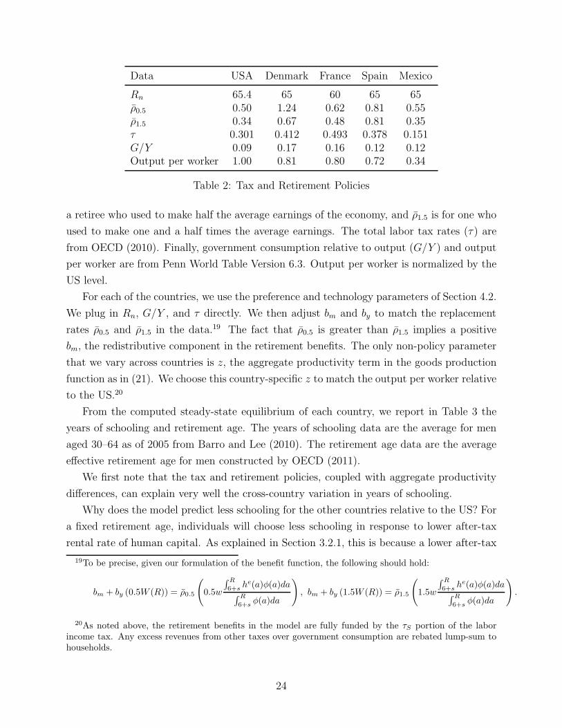
All the data in Table 2 are for 2005. The statutory full retirement age (Rn) and pension
replacement rates (ρ0.5 and ρ1.5) are from OECD (2011).18 The replacement rate ρ0.5 is for
17We report the results for Denmark, France, and Spain. Denmark and France are representative ofseveral other European countries. Spain is included as a sort of an outlier because our model prediction onretirement, using the tax and retirement systems summarized by the OECD, misses the data. We explainthis discrepancy below. The results for Germany are close to those for Denmark and France, and are notreported here.
18The US is in the process of gradually raising its full retirement age from 65 to 67, with the transition tobe completed when those born in 1960 turn 62 in 2022. This age was 65.4 as of 2005.
a retiree who used to make half the average earnings of the economy, and ρ1.5 is for one who
used to make one and a half times the average earnings. The total labor tax rates (τ) are
from OECD (2010). Finally, government consumption relative to output (G/Y ) and output
per worker are from Penn World Table Version 6.3. Output per worker is normalized by the
US level.
For each of the countries, we use the preference and technology parameters of Section 4.2.
We plug in Rn, G/Y , and τ directly. We then adjust bm and by to match the replacement
rates ρ0.5 and ρ1.5 in the data.19 The fact that ρ0.5 is greater than ρ1.5 implies a positive
bm, the redistributive component in the retirement benefits. The only non-policy parameter
that we vary across countries is z, the aggregate productivity term in the goods production
function as in (21). We choose this country-specific z to match the output per worker relative
to the US.20
From the computed steady-state equilibrium of each country, we report in Table 3 the
years of schooling and retirement age. The years of schooling data are the average for men
aged 30–64 as of 2005 from Barro and Lee (2010). The retirement age data are the average
effective retirement age for men constructed by OECD (2011).
We first note that the tax and retirement policies, coupled with aggregate productivity
differences, can explain very well the cross-country variation in years of schooling.
Why does the model predict less schooling for the other countries relative to the US? For
a fixed retirement age, individuals will choose less schooling in response to lower after-tax
rental rate of human capital. As explained in Section 3.2.1, this is because a lower after-tax
19To be precise, given our formulation of the benefit function, the following should hold:
bm + by (0.5W (R)) = ρ0.5
(0.5w
∫ R
6+she(a)φ(a)da
∫ R
6+sφ(a)da
), bm + by (1.5W (R)) = ρ1.5
(1.5w
∫ R
6+she(a)φ(a)da
∫ R
6+sφ(a)da
).
20As noted above, the retirement benefits in the model are fully funded by the τS portion of the laborincome tax. Any excess revenues from other taxes over government consumption are rebated lump-sum tohouseholds.
24
USA Denmark France Spain Mexico
Years of schooling (Data) 12.65 10.52 10.77 10.70 8.64Years of schooling (Model) 12.65 11.23 10.45 11.01 8.39
Retirement age (Data) 64.6 63.3 58.7 61.4 73.0Retirement age (Model) 64.6 63.5 60.0 65.0 65.0
Table 3: Schooling and Retirement (Data and Model)
rental rate implies relatively more expensive goods input to human capital production, which
results in less human capital investment overall. The after-tax rental rate of human capital
is lower in the other countries, because of higher taxes (in the case of Denmark, France, and
Spain) and of lower aggregate productivity (in the case of Denmark, Spain, and Mexico).
This effect also interacts with the retirement age. In Denmark and France, earlier re-
tirement implies a shorter horizon of human capital utilization, further discouraging human
capital investment and schooling.
The model performance is mixed when it comes to retirement decisions. For Denmark
and France, the picture is clear. These countries have higher labor income taxes than the
US, and also more generous transfers in terms of retirement benefits (bm and by) and non-
retirement rebates (u). In light of the first-order condition (19), these policies decrease the
numerator of the left-hand side and increase its denominator, with the overall impact of
lowering the retirement age. In the case of France, the model retirement age of 60 is actually
the corner (Rn) set by the retirement benefit program: If a French worker works past 60, the
forfeiture of his retirement benefits acts as an effective tax rate of 50 percent on his labor
income. In Section 4.3.2, we examine this case in more detail.
The model fails to explain the retirement decision of Spaniards: In the data, the retire-
ment age is 61.4, but the model predicts 65.21 We now explain why.
In our model, the full retirement age Rn causes a kink in the value of retirement, because
the worker’s forfeiture of retirement benefits from Rn on imposes an effective tax on continued
work. We set Rn = 65 for Spain, as reported in OECD (2011), and this happens to be the
retirement age in our model. However, for many countries, a kink is posed not only by the full
retirement age Rn, but also by the early retirement age. The early retirement age in Spain
is 61, and it is estimated that the effective tax rate in the form of the forfeited retirement
benefits for the average Spanish worker working past 61 is 35 percent (Duval, 2004). While
this is much smaller than the effective tax rate at the full retirement age—which is as high
as 90 percent in Spain—it is sizable enough to induce retirement for the majority of Spanish
21The model retirement age of 65 for Spain is also the corner set by the retirement benefit program. Therepresentative Spanish worker in the model would work for longer, were it not for this policy-induced kink.
25
workers in reality. Indeed, when we modify our retirement benefit function in Spain to
incorporate this early retirement age of 61, our model predicts that the average Spanish
worker retires at this very kink. However, to maintain consistency across our calibration
and counterfactual analyses, we choose to leave the early retirement age for Spain out of the
model.22
More interesting, even though the model underpredicts the retirement age in Mexico, it
shows that there is no inconsistency between fewer years of schooling and a higher retirement
age. Comparing Mexico and the US, Mexican workers have less schooling (by 4.26 years),
but retire 0.4 years later in the model.23 To understand this, one needs to consider the
non-retirement transfer u. While the total tax wedge τ is twice as high in the US as in
Mexico, government consumption relative to GDP is higher in Mexico. At the same time,
the social security programs, in terms of replacement rates and full retirement age, are
very similar in the two countries. Then, the government budget constraint implies that the
lump-sum non-retirement redistribution (u) is much smaller in Mexico. This explains why
Mexican workers may retire later in the model: Although the substitution effect from the
lower after-tax wage (owing to lower z) pushes retirement in the opposite direction (i.e.,
toward earlier retirement), the income effect from the smaller transfer prevails. We will see
this very intuition at work again in Section 4.3.4, when we consider the US circa 1900.
In summary, we find that our model can explain much of the cross-country difference
in schooling and retirement with the difference in their tax and retirement policies. The
shortcomings of our model regarding retirement in Spain and Mexico call for a richer model
that can better capture the relevant institutional details, which is left for future research.
Before moving on, we briefly discuss our model implications on another dimension: age-
earnings profiles. With the tax and retirement policies in the European countries we consider,
not only is there less schooling measured in years, but also less human capital accumulation
both in and out of school. In our model, this implies a flatter age-earnings profile. The
earnings between age 25 and 50 in the US from our model grow faster than in Spain by 37
percent and than in France by 90 percent. In other words, the age-earnings profiles in our
22Even if we were to model the early retirement age for all countries in our analysis, only our results onSpain will change. For Denmark and France, the early retirement age coincides with the full retirement age,although in France those who are disabled and long-term unemployed can apply for early retirement at theage of 58. For the US, the early retirement age is 62, but there is an actuarially-fair adjustments for thosewho claim benefits before the full retirement age. That is, there is no kink induced by the US retirementpolicy at the age of 62.
23The Mexican retirement age of 65 in the model is again the corner set by the retirement benefit program.Although we assume that all Mexican workers are subject to the tax and retirement policies, we are keenlyaware of the limited coverage of official pensions in Mexico, partly because of the vast informal sector. If wewere to take into account this limited coverage and remove the Rn = 65 corner, the Mexican workers in ourmodel will work for longer and our model will more closely match the retirement age in the data, 73.
26
model seem to be consistent with the steeper slopes observed in the US and the flatter slopes
in the European countries.24
4.3.2 Imposing the US Retirement Benefit Program on Other Countries
In this section, we evaluate the long-run effects of imposing the retirement benefit system
of the US on each of the other four countries. We hold all other parameters constant, and
re-calibrate Rn, bm, by, τS , and τ . We plug in Rn = 65.4, which is the US full retirement age,
and choose bm and by for each country to match the US replacement rates (ρ0.5 = 0.5033
and ρ1.5 = 0.3411). We maintain the assumption that the retirement benefit system pays
for itself with τS. Thus, we obtain a new τS for each country. We hold τI constant, which
means that τ ≡ τS + τI will have to change by as much as does τS for each country. The
first row of Table 4 shows this adjustment. In addition, lump-sum non-retirement transfers
(u) adjust to satisfy the government budget constraint.
We compute the resulting new steady states, and report in Table 4 the impact of this pol-
icy change on years of schooling (s), retirement age (R), career length (R−s−6), and output
per worker. We also compute the average human capital supplied to the labor market by a
worker, divided by years of schooling: he/s, where he ≡(∫ R
6+she(a)φ(a)da
)/(∫ R
6+sφ(a)da
).
This is a measure of human capital that is not fully captured by years of schooling. This
measure and output per worker are normalized by their respective levels in the US. The
change is indicated by the arrows from the initial steady states to the new steady states. We
note that the initial steady state values are from the model, as they do not perfectly fit the
data—see Table 3.
In the three European countries with generous retirement benefits and high taxes, the
US-style reform brings down τS and hence τ by more than ten percentage points. The social
security tax rates fall for two reasons. First, the new replacement rates are lower, and the
benefits can be financed with lower taxes. Second, workers are now eligible for benefits at an
older age, especially so in France, and hence the beneficiaries make up for a smaller fraction
of the population.
This is a significant cut in the total labor wedge τ , which increases schooling by one
full year (Spain) to more than two years (France), as explained in Section 3.2.1. In relative
24While longitudinal data that span such a long period are not easily accessible for most countries, wefound estimates for Spain (based on Spanish Social Security records) and Italy (based on the Bank of ItalySurvey on Household Income and Wealth), as well as for the US (based on Social Security records). For theparticular cohorts followed in these three countries, the average earnings in the US grow faster over the lifecycle than in Spain by 83 percent and than in Italy by 20 percent. The age-earnings profile constructed fromcross-sections also show that the US has a steeper slope than other European countries. See for exampleOECD (2006). However, we do not use this evidence, because the cross-section estimates confound age andcohort effects.
terms, years of schooling increase by 10 percent (Spain) to 23 percent (France).
In addition, workers now retire later. In all three countries, the new retirement age is
65.4, the corner in the US retirement benefit program. In the pre-reform steady states,
Danish workers were not at a corner, but their French and Spanish counterparts were. The
retirement age rises by two years in Denmark, and only by a half-year in Spain.25 The most
dramatic change, again, is in France. With the French workers previously at the Rn = 60
corner, they not only face a much lower tax but also a new corner that is much farther out
at Rn = 65.4. They now retire 5.4 years later. The later retirement reinforces the incentive
to acquire human capital driven by lower taxes, since it implies a longer horizon of human
capital utilization.
One important distinction that we make in our framework is the one between pure quan-
tity measures of raw labor supply (i.e., career length) and labor services measured in efficiency
units (i.e., effective labor). We now ask how workers respond along these two margins in
response to the reforms. It is clear from Table 4 that the model predicts only small changes
in career length. The number of years worked rises by a half-half year in Denmark and three
years in France, and actually declines by more than a half-year in Spain. This is because the
rise in retirement age is accompanied by increases in years of schooling—recall that career
length is R− (6+ s). These are small relative changes (Spain’s -1.5 percent to France’s +6.9
percent) in career length.
The big economic impact comes from the changes in human capital or the quality of
labor. Not only do workers now have more years of schooling, they also invest more in their
human capital both in and out of school. As a result, the average human capital supplied
to the labor market by a worker, he (not divided by years of schooling), rises by 15 percent
25As explained in Section 4.3.1, our model over-predicts the retirement age for Spain because we inten-tionally dismiss the early retirement kink at age 61. This is why the US-style reform has little impact onretirement in our model economy of Spain. When we incorporate the early retirement benefits, our modelretirement age for Spain is 61; in this case, the reform has a significant effect on retirement age, pushing itto 65.4.
28
(Spain) to 35 percent (France). The effective labor supplied per worker per year of schooling,
he/s, also rises by 4 percent (Spain) to 10 percent (France). Therefore, even if one proxies
human capital with years of schooling, the impact of the reform on human capital will still
be underestimated by a substantial margin—by one-third, to be more precise.
All the increased human capital accumulation translates into the substantial increase in
output per worker in the long run. With our goods production function, because the reforms
do not alter the ratio of physical capital to human capital (κ), the steady-state output per
worker increases one-to-one with the effective labor supplied per worker, as in equation (21):
by 15 percent (Spain) to 35 percent (France).26 To put this number in perspective, note that
the convergence to a steady state in this model takes approximately 40 years owing to the
demographic structure. The impact of the social security reform in Denmark and France is
tantamount to extra 0.45 and 0.75 percentage point growth per year, respectively, over 40
years.
For a decomposition of the economic impact via the raw labor and the human capital
channels, we consider the changes in output per capita, which is the product of output
per worker and the labor force participation rate—equations (21) and (22). For the three
countries, output per capita increases by 13 percent (Spain) to 39 percent (France). For
France, 35 percentage points out of the 39 come from the increase in human capital, and the
labor force participation channel accounts for the small remainder. As for the 13 percentage
points in Spain, 15 come from the human capital channel, while the labor force participation
channel negatively contributes to output per capita: In our exercise for Spain, years of
schooling rise by more than the retirement age, reducing the career length and hence the
labor force participation rate. Therefore, if one focuses only on the pure quantity measures
of raw labor supply (i.e., labor force participation rate or career length in this case), the
economic impact of the reforms will be grossly underestimated—or, what is worse, even
assigned the wrong sign.
In summary, we find that the adoption of a US-style retirement system in the three
European countries will significantly raise their output per worker, and most of the effect
materializes through the human capital channel, which is only partly captured by the increase
in years of schooling.
By contrast, a switch to the US-style retirement system has hardly any effect for Mexico,
since its retirement benefit system is largely similar to the US system to begin with.
26The model predicts that the new steady-state output per worker in France (1.08) is even higher thanthe US level (1.0). This is driven by our country-specific aggregate productivity estimate, z. Since Francehas much higher tax rates than the US to begin with, the model dictates that its z be higher in order tomatch the observed levels of output per worker. When its taxes are reduced, its output per worker happensto exceed the US level.
29
Before we move on to the next exercise, we consider the French case in more detail.
Adopting the US retirement benefit program for France involves two important changes.
One is the reduction in replacement rates, and the other is the increase in full retirement age
Rn, from 60 to 65.4. To get a sense of the relative importance of these two elements, we work
out an intermediate reform of raising Rn to 65.4 with the replacement rates left unchanged.27
In the new steady state associated with this intermediate reform, retirement age is 64.0 (from
60.0), years of schooling is 12.18 (from 10.45), and output per worker relative to the US is
0.99 (from 0.80). The average effective labor per year of schooling (he/s) is 0.97 (from 0.91).
We conclude that the increase in full retirement age from 60 to 65.4 alone accounts for about
two-thirds of the economic impact of the full reform in France. Again, the vast majority of
the economic impact operates through the human capital channel both in and out of school,
with the career length increasing by 2.27 years (or 5 percent).
4.3.3 Changes in Demographics and Tax/Retirement Policies
In this section we consider four experiments on the benchmark US economy. While these
experiments do have policy implications (e.g., raising the full retirement age to 67, which
is being gradually rolled out in the US), our main purpose is to further clarify the inner
workings of the model by considering one change at a time.
As for demographic changes, we consider the long-run impact of an increase in the life
span (T ) from 78 to 80. Holding all other parameters constant, we re-calibrate bm, by, and
τS to maintain the replacement rates and to balance the social security budget. Again, τ
will change one-to-one with τS, as τI is held constant. The results from the new steady state
are reported in the second column of Table 5.
The two-year increase in life span has small effects on labor market outcomes. All else
equal, a longer life span calls for a later retirement, as the worker needs to generate more
income to pay for the additional consumption later in life. This would by itself result in more
schooling, as the horizon for human capital utilization is now longer. However, in equilibrium,
taxes must rise (τS and hence τ by 1.7 percentage point) to support the longer-living retirees.
Through the channel explained in Section 3.2.1, this discourages human capital acquisition.
The effect of the higher taxes on retirement age can be ambiguous because of the opposing
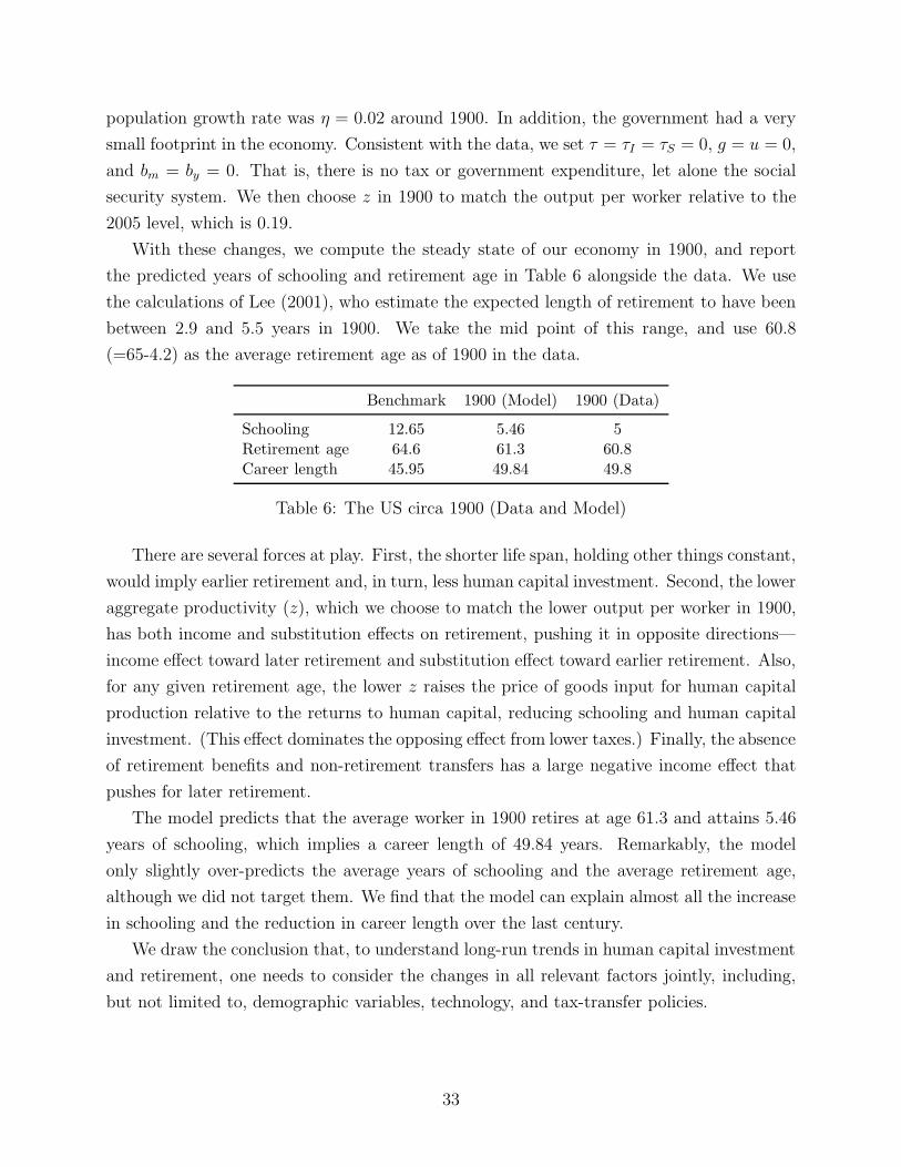
income and substitution effects. In the end, schooling decreases slightly (by less than a
month), but retirement age rises (by four months), lengthening the career by almost a half-
year. However, the smaller investment in human capital results in lower output per worker,
although the magnitude is very small.
27This requires a new calibration of Rn, τS , τ , bm, and by, except that now we pick bm and by to maintainthe previous replacement rates (ρ0.5 = 0.6175 and ρ1.5 = 0.4846) in the face of the changes in Rn, τS , and τ .
30
Benchmark T = 80 Rn = 67 ρ0.5 = ρ1.5 No Social Security
In the third column, starting from the benchmark US economy, we raise the full retirement
age from 65.4 to 67, while maintaining the replacement rates. In the benchmark, workers
in the US retire at age 64.6, and are not at the Rn = 65.4 corner. Thus, there is no direct
impact from pushing back this policy-induced corner. Still, now the retirement benefits are
paid for those 67 and older, and the social security tax can be lowered, along with the total
tax wedge τ . This policy implies a 1.66 percentage point drop in the labor tax rate. In the
new steady state, workers retire later and acquire more schooling, with the career length
increasing by slightly less than one percent. The 3.3% increase in output per worker reflects
the increased human capital investment in and out of school: Years of schooling rise by two
percent, and the effective labor supply per year of schooling increases by one percent. The
intuition is the exact reverse of the tax hike in Section 3.2.1.
The effect of this policy change is small, especially when compared with the impact of
the similar reform for France that we considered at the end of Section 4.3.2. There are
two reasons. First, the French (intermediate) reform pushes Rn from 60 to 65.4, while the
experiment for the US is only from 65.4 to 67. Second, more important, French workers in
our model are at the Rn = 60 corner prior to the reform. Therefore, the reform has a direct
impact on retirement age and human capital investment, in addition to the indirect effect
through the new, lower tax rates.
This policy change in the US will also affect the age-earnings profile. With more human
capital investment early in the career, age-earnings profile will get steeper. Indeed, we find
in the model that earnings between age 25 and 50 now grow 9 percent faster than in the
benchmark. There is empirical evidence that corroborates this finding: Neumark and Stock
(1999) exploit cross-state variation in the implementation of laws against age discrimination
in the US, and report that the age-earnings profile of young workers steepened with the
elimination of mandatory retirement.
In the fourth column, we remove the redistributive component of the social security by
setting bm = 0. We compute a new value of by that satisfies the social security budget
31
constraint with the same τS = 0.1116 as before. Hence, all tax rates remain the same. This
is very close to the bm − by exercise in Section 3.2.1, and here the obvious effect is the rise
in retirement age. In turn, the schooling period lengthens, as the horizon of human capital
utilization gets longer. The career length increases by 1.4 percent, and output per worker
also rises by 2 percent driven by the higher level of human capital.
Finally, we eliminate the social security system. In the model, this is done by setting
bm, by, and τS all equal to zero. The total labor tax wedge τ decreases by 0.1116 from
0.3010. In addition, Rn is now irrelevant. This experiment can be thought of an extreme
version of the second experiment above (third column), and hence the same logic—which
has been discussed in detail in Section 3.2.1—applies. We obtain sizable long-run effects
from this experiment. With much lower labor income taxes, workers acquire more human
capital in and out of school: Years of schooling increase by 12 percent, and the effective labor
supply per year of schooling rises by 9 percent. All in all, with the higher level of human
capital, output per worker rises by 23 percent. They also retire later, and their career length
increases, but only by 6 percent.
In summary, we again find that the reduction of distortions from taxes and retirement
benefits can have significant economic impact. Most of the effect materializes through an
increase in human capital investment both in and out of school. As a result, a pure quantity
measure of raw labor supply will significantly underestimate the true economic impact of
policy changes.
4.3.4 The US in 1900
As a final exercise, we ask whether our model can explain the trends in schooling and
retirement over time for the US. In 1900, more than 60 percent of men aged 65 or older were
in the labor force, while the figure in 2005 is 20 percent, with an average retirement age of
64.6.28 At the same time, the average years of schooling among adult males in the US in
1900 was 5 years, increasing to 12.65 by 2005. To summarize, over the past century, workers
acquired more and more human capital (as proxied by schooling), but their career length
shortened significantly.29
We cast our model in the year 1900 as follows. First, the life span was shorter in 1900.
We use the life expectancy at age 20, which implies a life span of T = 65 years.30 The
28According to Carter and Sutch (1996), only about a fifth of men who reached 55 eventually retired. Formany others, old age was a prolonged spell of unemployment, with the unemployment rate for those whowere 60 or older being estimated to exceed 30 percent.
29We use the estimates for schooling and output per worker in 1900 from Turner et al. (2007).30The number is from Bell and Miller (2005). The life expectancy at birth was merely 52 years. This large
discrepancy is explained by the high infant mortality rate in 1900. For our model, we find the expectancyat age 20 to be more relevant.
32
population growth rate was η = 0.02 around 1900. In addition, the government had a very
small footprint in the economy. Consistent with the data, we set τ = τI = τS = 0, g = u = 0,
and bm = by = 0. That is, there is no tax or government expenditure, let alone the social
security system. We then choose z in 1900 to match the output per worker relative to the
2005 level, which is 0.19.
With these changes, we compute the steady state of our economy in 1900, and report
the predicted years of schooling and retirement age in Table 6 alongside the data. We use
the calculations of Lee (2001), who estimate the expected length of retirement to have been
between 2.9 and 5.5 years in 1900. We take the mid point of this range, and use 60.8
(=65-4.2) as the average retirement age as of 1900 in the data.