Lifetime of Anthropogenic Climate Change: Millennial Time Scales of PotentialCO2 and Surface Temperature Perturbations

M. EBY, K. ZICKFELD, AND A. MONTENEGRO

School of Earth and Ocean Sciences, University of Victoria, Victoria, British Columbia, Canada

D. ARCHER

Department of the Geophysical Sciences, University of Chicago, Chicago, Illinois

K. J. MEISSNER AND A. J. WEAVER

School of Earth and Ocean Sciences, University of Victoria, Victoria, British Columbia, Canada

(Manuscript received 2 April 2008, in final form 15 September 2008)

ABSTRACT

Multimillennial simulations with a fully coupled climate–carbon cycle model are examined to assess the

persistence of the climatic impacts of anthropogenic CO2 emissions. It is found that the time required to absorb

anthropogenic CO2 strongly depends on the total amount of emissions; for emissions similar to known fossil

fuel reserves, the time to absorb 50% of the CO2 is more than 2000 yr. The long-term climate response appears

to be independent of the rate at which CO2 is emitted over the next few centuries. Results further suggest that

the lifetime of the surface air temperature anomaly might be as much as 60% longer than the lifetime

of anthropogenic CO2 and that two-thirds of the maximum temperature anomaly will persist for longer than

10 000 yr. This suggests that the consequences of anthropogenic CO2 emissions will persist for many millennia.

1. Introduction

The projection of the climatic consequences of anthro-

pogenic CO2 emissions for the twenty-first century has

been a major topic of climate research. Nevertheless, the

long-term consequences of anthropogenic CO2 remain

highly uncertain. The Intergovernmental Panel on Cli-

mate Change (IPCC) Fourth Assessment Report (AR4)

reported that ‘‘about 50% of a CO2 increase will be re-

moved from the atmosphere within 30 years and a further

30% will be removed within a few centuries’’ (Denman

et al. 2007, p. 501). Although the IPCC estimate of the

time to absorb 50% of CO2 is accurate for relatively small

amounts of emissions at the present time, this may be a

considerable underestimation for large quantities of

emissions. Carbon sinks may become saturated in the fu-

ture, reducing the system’s ability to absorb CO2.

Atmospheric CO2 is currently the dominant anthro-

pogenic greenhouse gas implicated in global warming

(Forster et al. 2007); therefore, estimating the lifetime

of anthropogenic climate change will largely depend on

the perturbation lifetime of CO2. The perturbation

lifetime is a measure of the time over which anomalous

levels of CO2 or temperature remain in the atmosphere

(defined here to be the time required for a fractional

reduction to 1/e). Carbon emissions can be taken up

rapidly by the land, through changes in soil and vege-

tation carbon, and by dissolution in the surface ocean.

Ocean uptake slows as the surface waters equilibrate

with the atmosphere and continued uptake depends on

the rate of carbon transport to the deep ocean. Ocean

uptake is enhanced through dissolution of existing

CaCO3, often referred to as carbonate compensation.

As CO2 is taken up, the ocean becomes more acidic,

eventually releasing CaCO3 from deep sediments. This

increases the ocean alkalinity, allowing the ocean to

take up additional CO2. Carbonate compensation be-

comes important on millennial time scales, whereas

changes in the weathering of continental carbonate and

Corresponding author address: M. Eby, School of Earth and

Ocean Sciences, University of Victoria, P.O. Box 3055, Victoria,

BC V8W 3P6, Canada.

E-mail: eby@uvic.ca

VOLUME 22 J O U R N A L O F C L I M A T E 15 MAY 2009

DOI: 10.1175/2008JCLI2554.1

� 2009 American Meteorological Society 2501

silicate are thought to become important on the 10 000–

100 000-yr time scale (Archer 2005; Sarmiento and

Gruber 2006; Lenton and Britton 2006).

Earth system models can be used to simulate the ev-

olution of the climate system under different anthro-

pogenic emissions scenarios. There is still a great deal of

uncertainty in the climate–carbon cycle response and

considerable variation in model predictions. The short

term (century time scale) may be dominated by the

terrestrial carbon cycle response, which is poorly un-

derstood. Over the longer term (millennial time scale)

the ocean biology, sediment, and weathering responses

are also highly uncertain. Comprehensive model simu-

lations of the next few centuries suggest that CO2

anomalies may be relatively long lived (Friedlingstein

et al. 2006; Plattner et al. 2008). These studies also

illustrate the large uncertainties in the modeled short-

term carbon cycle response but they were not designed

to estimate the multimillennial response or the de-

pendency of the recovery time scales on the level of

emissions.

There are few modeling studies that have consid-

ered the coupled climate–carbon cycle response to

large anthropogenic emissions on the 10 000-yr time

scale. Differing levels of complexity and experimental

design make a detailed comparison of other studies

difficult, but most studies suggest that the average

perturbation lifetime of most of the CO2 is on the

order of a few centuries and that as much as a quarter

of the perturbation lasts for more than 5000 yr (Archer

et al. 1998; Archer 2005; Archer and Brovkin 2008;

Lenton and Britton 2006; Lenton et al. 2006; Ridgwell

and Hargreaves 2007; Ridgwell et al. 2007; Mikolajewicz

et al. 2007; Tyrell et al. 2007; Montenegro et al. 2007).

None of these studies attempted to estimate the millen-

nial time scales of the temperature response or investi-

gated the multimillennial response as a function of the

magnitude of the perturbation in a systematic way.

Models that have looked at the long-term carbon

cycle response are usually low resolution, highly pa-

rameterized, or incomplete. For example, Archer

(2005) used highly parameterized climate feedbacks,

whereas Montenegro et al. (2007) used two incomplete

models: one model lacked a terrestrial carbon cycle and

the other lacked ocean sediments. The model used here

is currently one of the more complex coupled climate–

carbon cycle models capable of looking at multimil-

lennial time scales. Even given the large range in ex-

isting model predictions, we will show that the lifetime

of both the anthropogenic CO2 perturbation and the

resulting surface air temperature (SAT) change may be

longer than previously thought.

2. Model description and evaluation

We use version 2.8 of the University of Victoria (UVic)

Earth System Climate Model (ESCM). It consists of a

primitive equation 3D ocean general circulation model

with isopycnal mixing and a Gent and McWilliams (1990)

parameterization of the effect of eddy-induced tracer

transport. For diapycnal mixing, a horizontally constant

profile of diffusivity is applied, with values of about

0.3 1024 m2 s21 in the pycnocline. The ocean model is

coupled to a dynamic–thermodynamic sea ice model and

an energy–moisture balance model of the atmosphere

with dynamical feedbacks (Weaver et al. 2001). The land

surface and terrestrial vegetation components are rep-

resented by a simplified version of the Hadley Centre

Met Office surface exchange scheme (MOSES) coupled

to the Top-down Representation of Interactive Foliage

and Flora Including Dynamic vegetation model; Meissner

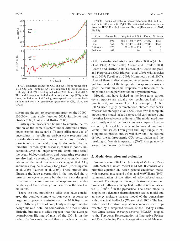
FIG. 1. Historical changes in CO2 and SAT. (top) Model simu-

lated CO2 and (bottom) SAT are compared to historical data

(Ethridge et al. 1998; Keeling and Whorf 2005; Jones et al. 2008).

The model simulation includes all historical forcings (CO2 emis-

sions, insolation, orbital forcing, tropospheric and stratospheric

sulfates and non-CO2 greenhouse gases such as CH4, N2O, and

CFCs).

TABLE 1. Simulated global carbon inventories in 1800 and 1994

and their differences (in PgC). The estimated values are taken

from the IPCC Fourth Assessment Report (Denman et al. 2007,

Fig 7.3).

Year Atmosphere Vegetation 1 Soil Ocean Sediment

1800 591 604 1 1366 5 1970 37 237 1166

1994 761 661 1 1437 5 2098 37 340 1166

Difference 170 57 1 71 5 128 103 0

Estimate 165 101 118 0

2502 J O U R N A L O F C L I M A T E VOLUME 22

et al. 2003). Land carbon fluxes are calculated within

MOSES and are allocated to vegetation and soil carbon

pools (Matthews et al. 2004). Ocean carbon is simulated

by means of an Ocean Carbon-Cycle Model Intercom-

parison Project type inorganic carbon cycle model and a

nutrient–phytoplankton–zooplankton–detritus marine

ecosystem model (Schmittner et al. 2008). Sediment

processes are represented using an oxic-only model of

sediment respiration (Archer 1996a).

An earlier version of the UVic ESCM (version 2.7)

has undergone extensive evaluation as part of inter-

national model intercomparison projects including the

Coupled Carbon Cycle Climate Model Intercomparison

Project (Friedlingstein et al. 2006), the Paleoclimate

Modeling Intercomparison Project (Weber et al. 2007),

and the coordinated thermohaline circulation experi-

ments (Gregory et al. 2005; Stouffer et al. 2006). The

model has also been used for multicentury climate

projections in support of the IPCC Fourth Assessment

Report (Denman et al. 2007; Meehl et al. 2007). Here,

we evaluate the UVic ESCM version 2.8 primarily with

respect to its ability to simulate characteristics of the

coupled climate–carbon cycle system, including the air–

sea flux of CO2, the distribution of ocean dissolved in-

organic carbon (DIC) and alkalinity, the percent of

CaCO3 in sediments, the global carbon budgets of the

last decades and the observation-based evolution of sur-

face air temperature and CO2 over the historical period.

From a preindustrial climate, this version of the model

has a transient climate response of 2.08C and an equilib-

rium climate sensitivity of 3.58C (Weaver et al. 2007).

The simulated evolution of atmospheric CO2 and

surface air temperature over the historical period is in

good agreement with observations (Fig. 1). For the year

2000, the simulated CO2 is about 5 ppmv higher than the

observation-based value. The model does not produce

as much interannual variability as seen in the data but

the long-term trends are well reproduced. Warming

over the twentieth century is 0.78C, in agreement with

the IPCC estimate of 0.68 6 0.28C (Forster et al. 2007).

The simulated inventories of carbon in the atmos-

phere, ocean, and on land in the years 1800 and 1994

and their difference are given Table 1. The changes in

carbon inventories over the historical period (1800–

1994) compare relatively well with IPCC AR4 estimates

(1750–1994). The observation-based changes in carbon

reservoirs during the 1980s, 1990s, and 2000–05 are well

reproduced by the model (Table 2). The atmospheric

CO2 increase is in close agreement with observations for

the 1980s and 2000–05 but is overestimated in the 1990s.

Ocean CO2 uptake agrees very well with the observation-

based values, but for a slight overestimation in 2000–05.

Land CO2 uptake falls well within the estimated un-

certainty range for all time periods and is close to the

IPCC best estimate.

The model reproduces qualitatively and quantita-

tively most features of the observation-based patterns of

TABLE 2. Modeled and estimated global carbon budgets are for the 1980s, 1990s, and 2000–05 in PgC yr21. The estimated values are taken

from the IPCC Fourth Assessment Report (Denman et al. 2007, Table 7.1).

1980s 1990s 2000–05

Model Estimate Model Estimate Model Estimate

Atmospheric increase 3.3 3.3 6 0.1 3.7 3.2 60.1 4.2 4.1 6 0.1

Ocean uptake 21.8 21.8 6 0.8 22.2 22.2 6 0.4 22.4 22.2 6 0.5

Land uptake 22.2 21.7 (23.4 to 0.2) 22.6 22.6 (24.3 to 20.9) 22.8 n/a

FIG. 2. Air–sea flux of carbon. (top) Model simulated fluxes at

the year 2000 compared with (bottom) observational estimates

(Takahashi et al. 2009). Negative values denote ocean uptake.

15 MAY 2009 E B Y E T A L . 2503

air–sea exchange of CO2 (Fig. 2). These features include

outgassing in low latitudes with a maximum in the

eastern tropical Pacific and uptake at mid- and high

latitudes with maxima around 408N–S in the areas of the

North Atlantic Current, the Kuroshio Current, and the

Southern Ocean. Model biases include underestimated

uptake in the Greenland–Iceland–Norwegian Seas

and overestimated uptake in the eastern subtropical

Pacific.

The simulated patterns of DIC and alkalinity show

good agreement with observations (Figs. 3, 4). The

model captures well the surface to deep gradient of both

tracers. At depth the model slightly underestimates

carbon while slightly overestimating alkalinity. See

Table 3 for a summary of the average values and ab-

solute errors of simulated DIC and alkalinity for the

global, Arctic–Atlantic, and Indo-Pacific oceans. The

simulated patterns of CaCO3 are also in reasonable

agreement with observations (Fig. 5). Nevertheless, the

model underestimates deep CaCO3 at tropical latitudes

and overestimates CaCO3 at high latitudes. Comparing

only locations with observations, the global average

percent of CaCO3 in sediments is 34.5% for the data

and 31.1% for the model.

3. Experimental design

The model was spun up for 10 000 yr with atmospheric

carbon dioxide levels and Earth’s orbital configuration

specified for the year 1800 and the continental CaCO3

weathering flux diagnosed from the ocean sediment

burial flux. The weathering flux was then held fixed

while the burial flux of CaCO3 was allowed to evolve

with time for all subsequent experiments. Historical

emissions were applied until the end of the year 2000.

These historical CO2 emissions include contributions

from both fossil fuel burning and land use changes. All

other transient forcings (insolation, orbital forcing,

tropospheric and stratospheric sulfates, and non-CO2

greenhouse gases such as CH4, N2O, and CFCs) were

held fixed.

At the beginning of 2001, ‘‘pulses’’ of CO2 were ap-

plied over 1 yr. The emissions varied from 160 PgC

(1015 g of carbon) to 5120 PgC (Table 4). The upper

bound approximates all known conventional fossil fuel

reserves (Rogner 1997). In addition to the pulse ex-

periments, we also performed simulations with more

‘‘realistic’’ emissions scenarios. As a baseline, we as-

sumed that emissions follow the A2 scenario up to the

FIG. 3. (top) Model simulated zonally averaged DIC at the year 1994 compared with (bottom) GLODAP data (Key

et al. 2004) for (left) Arctic–Atlantic and (right) Indo-Pacific oceans.

2504 J O U R N A L O F C L I M A T E VOLUME 22

year 2100 and then decline linearly to zero by 2300. This

scenario is designated as A21 (Montenegro et al. 2007).

We then generated a set of scenarios in which the A21

emissions were scaled such that the cumulative emis-

sions reached those of the equivalent pulse simulation

by the year 2300. A21 and pulse simulations were in-

tegrated for 5000 and 10 000 model years, respectively.

To explore the consequences of future emissions only, a

10 000-yr control simulation was also carried out with

zero emissions after the year 2000. At the end of this

integration the SAT was again at its year 2000 value

(having dropped 0.18C from its temporary maximum)

whereas CO2 had dropped by 55 ppmv to 321 ppmv.

These control results are subtracted from the results of

the future emissions experiments.

4. Discussion and conclusions

Resulting maximum changes in atmospheric CO2

range from 26 to 2352 ppmv (Fig. 6; Table 4). In the

pulse experiments, the maximum CO2 anomaly occurs

at the beginning, initially decaying very rapidly but

slowing after several decades. In the A21 experiments,

atmospheric CO2 peaks a few decades before the year

emissions are set to zero (260–286 yr; Table 4). After the

peak, CO2 closely approaches the level of the corre-

sponding pulse experiment after about 500 yr. This

demonstrates that the long-term atmospheric CO2 re-

sponse is nearly independent of the rate of CO2

emissions (assuming all emissions occur over the next

300 yr).

FIG. 4. (top) Model simulated zonally averaged alkalinity at the year 1994 compared with (bottom) GLODAP data

(Key et al. 2004) for (left) Arctic–Atlantic and (right) Indo-Pacific oceans.

TABLE 3. Model (M), data estimate (D; Key et al. 2004), and absolute error (E) for DIC and Alkalinity averaged over the Global,

Arctic–Atlantic, and Indo-Pacific oceans for the year 1994.

Global Arctic–Atlantic Indo-Pacific

M D E M D E M D E

DIC (mol m23) 2.291 2.309 0.022 2.233 2.246 0.019 2.311 2.331 0.023

Alkalinity (mol m23) 2.424 2.421 0.014 2.396 2.392 0.012 2.434 2.431 0.014

15 MAY 2009 E B Y E T A L . 2505

A considerable amount (15%–30%) of the atmo-

spheric CO2 anomaly persists at the end of the 10 000-yr

simulations (Fig. 6). The time to absorb a given percent

of emissions is strongly dependent on the total amount

of emissions (Fig. 7; Table 4). For emissions up to about

1000 PgC, 50% of the CO2 anomaly is taken up within

100 yr and another 30% is absorbed within 1000 yr,

which is similar to IPCC estimates (Denman et al. 2007).

Above 1000 PgC, the time to absorb 50% of the emissions

increases dramatically, and more than 2000 yr are needed

to absorb half of a 5000-PgC perturbation.

Ocean surface pH is strongly coupled to atmospheric

CO2 (Caldeira and Wicket 2003). Emissions above 1280

PgC result in a decrease in average ocean surface pH

that is larger than the 0.2 guard rail proposed by the

German Advisory Council on Global Change (WGBU;

Schubert et al. 2006; Fig. 8). Given the slow decay of

atmospheric CO2, experiments with emissions of 2560

PgC and larger still have lower pH than the 0.2 guard

rail after 10 000 yr. For high emissions, the change in

surface pH would probably have a significant impact on

oceanic biota. Emissions of 1920 PgC and above result

in minimum pH levels below 7.9, a value that could

bring the aragonite saturation depth to the surface in

the Southern Ocean generating serious adverse effects

on calcifying organisms (Orr et al. 2005).

There is a lag in the response of surface air temper-

ature to the CO2 forcing (Fig. 9). For all but the lowest

emissions, temperature reaches its maximum at least

550 yr after the peak in atmospheric CO2 (Table 4). The

lag is particularly pronounced in the experiments with

FIG. 5. (top) Model simulated percent dry weight CaCO3 at year

2000 compared with (bottom) coretop data (Archer 1996b). Note

that only locations with data are shown in both panels to facilitate

the comparison.

TABLE 4. Level and year of maximum CO2 (Max CO2), first year at which 50% of total emissions have been absorbed from the

atmosphere (50% emissions), level and year of maximum SAT (Max SAT), and the first year at which SAT is less than 80% of the

maximum (80% max SAT).

Max CO2 Max SAT

Expt (Pg) (ppmv) (yr) 50% emissions (yr) (8C) (yr) 80% max SAT (yr)

160 69 1 18 0.32 247 527

160_A21 26 270 187 0.32 342 1787

320 139 1 23 0.61 110 2230

640 280 1 36 1.38 3519 4363

640_A21 118 260 201 1.40 3357 4153

960 423 1 63 2.00 2047 3126

1280 568 1 105 2.55 1965 3521

1280_A21 274 269 232 2.53 2110 3583

1920 859 1 218 3.70 1147 3441

2560 1155 1 428 4.75 715 3929

2560_A21 699 278 520 4.72 832 3943

3200 1453 1 781 5.66 809 4441

3840 1752 1 1309 6.48 1076 5066

3840_A21 1223 284 1388 6.43 1147 4986

4480 2051 1 1732 7.24 1085 5248

5120 2352 1 2151 7.86 971 6190

5120_A21 1781 286 2210 7.82 1287 .5000

2506 J O U R N A L O F C L I M A T E VOLUME 22

FIG. 6. Temporal changes in CO2. Differences (top) relative to

the control and (bottom) in terms of the percentage of CO2

emissions remaining in the atmosphere. Note the different scales

along the time axis. Colors indicate total emissions, with solid lines

for pulse scenarios and dotted lines for equivalent A21 scenarios.

FIG. 7. Percentages of anomalies remaining: (top) CO2 and

(bottom) SAT. Stars indicate experimental points and lines are just

visual aids. Note the different scales along the time axis and that

colors indicate different percentages remaining, not total emissions,

as in Figs. 6, 8, 9. For clarity, results for equivalent A21 scenarios

are not shown. The SAT anomaly is noisy for low emissions due

to long time-scale climate variability (see Fig. 9 and text).

FIG. 8. Temporal changes in sea surface pH. (top) Differences

relative to the control simulation and (bottom) differences in

terms of the percentage of the maximum pH anomaly remaining.

Note the different scales along the time axis. Colors indicate total

emissions, with solid lines for pulse scenarios and dotted lines for

equivalent A21 scenarios. Results for equivalent A21 scenarios

are not shown in the bottom panel for clarity.

FIG. 9. Temporal changes in SAT. Differences (top) relative to

the control and as a percentage of the maximum SAT anomaly for

(middle) high and (bottom) low emissions. High and low emissions

are plotted separately for clarity. Note the different scales along

the time axis. Colors indicate total emissions, with solid lines for

pulse scenarios and dotted lines for equivalent A21 scenarios.

15 MAY 2009 E B Y E T A L . 2507

total emissions in the range 640–1280 PgC, where after

2000–3500 yr, the planetary cooling is suddenly reversed

and SAT again increases by as much as 0.58C. This

abrupt warming and accompanying increase in CO2 is

caused by flushing events in the Southern Ocean, which

in this model have been shown to be dependent on the

level of atmospheric CO2 (Meissner et al. 2008). Under

the A21 emissions scenarios, the peak in SAT is almost

identical to the corresponding pulse experiments, indi-

cating that the long-term temperature response is in-

dependent of the rate of CO2 emissions (Fig. 9; Table 4).

The SAT anomaly is even longer lived than the CO2

anomaly. For all experiments, at least 50% of the

maximum temperature anomaly persists at the end of

the simulation. For both the smallest and largest emis-

sion scenarios, the temperature anomaly remaining af-

ter 10 000 yr is about 75% of the maximum anomaly.

Similar to CO2, the time to reduce temperature by a

specific percent of the maximum anomaly depends

on the total amount of emissions. The time within which

SAT declines by 20% relative to the peak warming

ranges from about 500 yr for the lowest emission sce-

nario to more than 5000 yr for the highest emissions

scenarios (Fig. 7; Table 4).

Given that the change in temperature from prein-

dustrial to the year 2000 is about 0.88C (Fig. 1), total

emissions of 640 PgC or more result in average air

temperatures above the 28C temperature guard rail

suggested by the WBGU (Schubert et al. 2006) and

endorsed by the European Union. The threshold to stay

below this guard rail would appear to be near 640 PgC

of total emissions from the year 2000. Experiments with

emissions of 1280 PgC and larger still exceed the 28C

guard rail after 10 000 yr.

To estimate the perturbation lifetime of anthropo-

genic climate change the response curves of either CO2

or temperature were fit to an exponential formula of the

form A0exp(2t/A1) 1 A2. The parameter A0 gives an

estimate of the amount a quantity is reduced, A1 is the

average lifetime, and A2 is the amount of any very long-

lived residual. We restrict our analysis to experiments with

total emissions greater than 1500 PgC. In simulations with

lower emissions, the response curve is often contaminated

by noise, making curve fitting imprecise (Figs. 6, 9).

A gradient-expansion algorithm was used to compute

the least squares fit of an exponential model to the data.

To tease out a fast and slow time scale for uptake of CO2,

an exponential fit was first applied to the CO2 curves

after 1000 yr. The data fit an exponential very well (see

Fig. 10). This curve was then extrapolated back 1000 yr

and the extrapolated CO2 was subtracted from the sim-

ulated CO2. A second exponential fit was performed on

the remaining CO2. This fit is clearly not as good as the

previous fit (Fig. 10). The early response is not a pure

exponential but a combination of processes with differ-

ent time scales (Joos et al. 1996). Still, this analysis

FIG. 10. Curve fitting to a double exponential model. Dotted

lines are an exponential fit to simulated CO2 after 1000 yr and are

used to estimate the slow time scale for reducing CO2 (slow).

These curves were extrapolated back 1000 yr and the extrapolated

CO2 was subtracted from the simulated CO2. A second exponen-

tial fit was performed on the remaining CO2 to estimate a fast time

scale for reducing CO2 (fast). The dashed curves are the sum of

two exponential curves (fast 1 slow). Note the different scales

along the time axis.

TABLE 5. Average perturbation lifetimes in years and percentages reduced. The average perturbation lifetimes are calculated from

exponential fits to model results. Percentages are of either total CO2 emissions or maximum SAT. All are calculated from differences

with the control (control has zero emissions from year 2001 onward).

CO2 SAT

Fast Slow Slow

Expt (Pg) (years) (%) (yr) (%) �10 000 yr (%) (yr) (%) �10 000 yr (%)

1920 146 56 3000 24 20 3400 39 61

2560 149 50 3000 28 22 3900 37 63

3200 136 43 2700 33 24 3900 34 66

3840 129 36 2900 38 26 4300 34 66

4480 102 29 2600 43 28 4100 31 69

5120 107 27 2900 44 29 4600 31 69

2508 J O U R N A L O F C L I M A T E VOLUME 22

provides a reasonable, if somewhat uncertain, estimate

of the overall fast absorption time scale. Although the

estimated short-term-response time scale may be de-

pendent on the number of exponentials used in the fit

(Maier-Reimer and Hasselmann 1987), the longer re-

sponse time scale (after 1000 yr) is quite robust and

reasonably independent of the section of the curve used

in the fit. The perturbation lifetime of CO2 is thus broken

up into a period of rapid absorption, a period of slow

absorption, and a ‘‘residual’’ that represents CO2, which

stays in the atmosphere for longer than this method can

resolve (�10 000 yr). To derive a perturbation lifetime

for temperature, we also fit an exponential model to

the temperature response curves after the year 1000.

We find that the response curves for CO2 can be well

approximated by the superposition of exponentials with

two different time scales. The average lifetime for the

short time scale is about 130 yr whereas the long time

scale has an average lifetime closer to 2900 yr (Table 5).

The amount of CO2 absorbed by processes associated

with the short time-scale sink are nearly constant (1075–

1382 PgC; calculated from Table 5). About 400 PgC of

the short time-scale sink is associated with increased

land uptake (mostly through CO2 fertilization), whereas

the rest (;900 PgC) are due to relatively rapid disso-

lution in the surface ocean (Fig. 11). The longer time

scale of the deep-ocean sink is associated with slow rates

of deep-ocean transport and carbonate dissolution. The

amount taken up by the deep-ocean sink is not constant

but increases at higher levels of emissions, implying that

the sink is not saturated. The absorption time scale for

CO2 does not seem to be very sensitive to the amount of

emissions (Table 5).

For high-emission experiments, after year 1000 (roughly

the year of maximum temperature), a single exponential

fits the temperature response very well. The average

perturbation lifetime is about 4000 yr, or 40% longer

than the average for CO2. The temperature perturba-

tion lifetime also appears to be more dependent on the

level of total emissions than the CO2 perturbation life-

time (Table 4).

Radiative forcing from atmospheric CO2 depends on

the logarithm of CO2, but for the first 1000 yr, the

thermal inertia of the ocean and climate feedbacks are

important in keeping SAT below what would be ex-

pected from the radiative forcing alone (Meehl et al.

2007). After 1000 yr, the time scale for reducing SAT

becomes very similar to the time scale of the CO2 ra-

diative forcing and this time scale is considerably longer

than for CO2. The logarithmic dependence of the radi-

ative forcing on CO2 is also why the SAT perturbation

lifetime depends on the total amount of emissions, even

though the time scale of CO2 absorption itself appears

to be relatively constant.

Figure 12 shows the portion of CO2, radiative forcing

from CO2, and surface temperature normalized to their

values at 1500 yr. The spread in the time scales for

CO2 (illustrated by the spread in the curves) is relatively

small and larger emissions seem to show slightly shorter

time scales (steeper slopes) than smaller emissions (also

see Table 5). Radiative-forcing time scales are longer

than for CO2 alone and, as with temperature, the time

scale for the decay of the radiative forcing increases as

emissions increase. The temperature time-scale depen-

dency on emissions can mostly be explained by the

changes in radiative-forcing time scales, although other

feedbacks make the spread in temperature time scales

even larger.

FIG. 12. Portion of anomalous CO2, radiative forcing, and sur-

face temperature relative to 1500 yr after the start of the simula-

tion. Although sometimes indistinct in the figure, the radiative

forcing and temperature curves are similar: both show longer time

scales (decline less steeply) than CO2 and time scales become

longer as emissions increase.

FIG. 11. Temporal changes in carbon pools. Differences in car-

bon relative to the control simulation for the 2560-PgC pulse ex-

periment. The sediment pool includes changes due to continental

weathering. Note the different scales along the time axis.

15 MAY 2009 E B Y E T A L . 2509

In summary, this study suggests that for emissions less

than about 1500 PgC, most of the CO2 will be absorbed

within a few centuries, which is in agreement with ear-

lier work. Temperature anomalies may last much lon-

ger. With larger emissions, the time to absorb most of

the CO2 increases rapidly (Table 4; Fig. 7). This de-

pendency of the CO2 response on the level of emissions

has important policy implications and needs to be in-

vestigated with other models. A long-term model in-

tercomparison project (LTMIP) with standardized ex-

periments has recently been initiated and this will

hopefully further increase our understanding and re-

duce the uncertainty in the long-term carbon cycle re-

sponse. Preliminary results from nine models (including

the one used here) can be found in Archer et al. (2009).

Although the long-term climate–carbon cycle re-

sponse still remains highly uncertain, the model used in

this study suggests that for large emissions, the pertur-

bation lifetime of both CO2 and surface temperature

might be longer than previously thought. The long-term

climate response appears to be independent of the rate

at which CO2 is emitted over the next few centuries.

Regardless of the future emissions trajectory, changes

to the earth’s climate will likely persist for several

thousands of years. The logarithmic relationship be-

tween CO2 and its radiative forcing implies that the time

scale at which atmospheric temperature declines will be

longer than the time scale of CO2. For ecosystems

having already adapted to a warmer world, slow cooling

may be beneficial. Nevertheless, it is sobering to ponder

the notion that the carbon we emit over a handful of

human lifetimes may significantly affect the earth’s cli-

mate over tens of thousands of years.

REFERENCES

Archer, D., 1996a: A data-driven model of the global calcite ly-

socline. Global Biogeochem. Cycles, 10, 511–526.

——, 1996b: An atlas of the distribution of calcium carbonate in

sediments of the deep sea. Global Biogeochem. Cycles, 10,

159–174.

——, 2005: Fate of fossil fuel CO2 in geologic time. J. Geophys.

Res., 110, C09S05, doi:10.1029/2004JC002625.

——, and V. Brovkin, 2008: The millennial atmospheric life-

time of anthropogenic CO2. Climatic Change, 90, 283–297,

doi:10.1007/s10584-008-9413-1.

——, H. Kheshgi, and E. Maier-Reimer, 1998: Dynamics of fossil

fuel CO2 neutralization by marine CaCO3. Global Biogeochem.

Cycles, 12, 259–276.

——, and Coauthors, 2009: Atmospheric lifetime of fossil-fuel

carbon dioxide. Annu. Rev. Earth Planet. Sci., 37, 117–134.

Caldeira, K., and M. E. Wickett, 2003: Anthropogenic carbon and

ocean pH. Nature, 425, 365.

Denman, K. L., and Coauthors, 2007: Couplings between changes

in the climate system and biogeochemistry. Climate Change

2007: The Physical Science Basis, S. Solomon et al., Eds.,

Cambridge University Press, 589–662.

Etheridge, D. M., L. P. Steele, R. L. Langenfelds, R. J. Francey,

J.-M. Barnola, and V. I. Morgan, 1998: Historical CO2 rec-

ords from the Law Dome DE08, DE08-2, and DSS ice cores.

Trends: A Compendium of Data on Global Change, Carbon

Dioxide Information Analysis Center. [Available online at

http://cdiac.esd.ornl.gov/trends/co2/lawdome.html.]

Forster, P., and Coauthors, 2007: Changes in atmospheric con-

stituents and in radiative forcing. Climate Change 2007: The

Physical Science Basis, S. Solomon et al., Eds., Cambridge

University Press, 129–234.

Friedlingstein, P., and Coauthors, 2006: Climate–carbon cycle

feedback analysis: Results from the C4MIP model intercom-

parison. J. Climate, 19, 3337–3353.

Gent, P. R., and J. C. McWilliams, 1990: Isopycnal mixing in ocean

circulation models. J. Phys. Oceanogr., 20, 150–155.

Gregory, J. M., and Coauthors, 2005: A model intercomparison of

changes in the Atlantic thermohaline circulation in response

to increasing atmospheric CO2 concentration. Geophys. Res.

Lett., 32, L12703, doi:10.1029/2005GL023209.

Jones, P. D., D. E. Parker, T. J. Osborn, and K. R. Briffa, 2008:

Global and hemispheric temperature anomalies—Land and

marine instrumental records. Trends: A Compendium of Data

on Global Change, Carbon Dioxide Information Analysis

Center. [Available online at http://cdiac.ornl.gov/trends/temp/

jonescru/jones.html.]

Joos, F., M. Bruno, R. Fink, U. Siegenthaler, T. F. Stocker, and

C. LeQuere, 1996: An efficient and accurate representation

of complex oceanic and biospheric models of anthropogenic

carbon uptake. Tellus, 48B, 397–417.

Keeling, C. D., and T. P. Whorf, 2005: Atmospheric CO2 records

from sites in the SIO air sampling network. Trends: A Com-

pendium of Data on Global Change, Carbon Dioxide Informa-

tion Analysis Center. [Available online at http://cdiac.ornl.gov/

trends/co2/sio-keel.html.]

Key, R. M., and Coauthors, 2004: A global ocean carbon climatol-

ogy: Results from Global Data Analysis Project (GLODAP).

Global Biogeochem. Cycles, 18, GB4031, doi:10.1029/

2004GB002247.

Lenton, T. M., and C. Britton, 2006: Enhanced carbonate and

silicate weathering accelerates recovery from fossil fuel CO2

perturbations. Global Biogeochem. Cycles, 20, GB3009,

doi:10.1029/2005GB002678.

——, and Coauthors, 2006: Millennial timescale carbon cycle and

climate change in an efficient Earth system model. Climate

Dyn., 26, 687–711.

Maier-Reimer, E., and K. Hasselmann, 1987: Transport and stor-

age of CO2 in the ocean—An inorganic ocean-circulation

carbon cycle model. Climate Dyn., 2, 63–90.

Matthews, H. D., A. J. Weaver, K. J. Meissner, N. P. Gillett, and

M. Eby, 2004: Natural and anthropogenic climate change: In-

corporating historical land cover change, vegetation dynamics

and the global carbon cycle. Climate Dyn., 22, 461–479.

Meehl, G. A., and Coauthors, 2007: Global climate projections.

Climate Change 2007: The Physical Science Basis, S. Solomon

et al., Eds., Cambridge University Press, 747–845.

Meissner, K. J., A. J. Weaver, H. D. Matthews, and P. M. Cox, 2003:

The role of land surface dynamics in glacial inception: A

study with the UVic Earth System model. Climate Dyn., 21,

515–537.

——, M. Eby, A. J. Weaver, and O. A. Saenko, 2008: CO2

threshold for millennial-scale oscillations in the climate

system: Implications for global warming scenarios. Climate

Dyn., 30, 161–174.

2510 J O U R N A L O F C L I M A T E VOLUME 22

Mikolajewicz, U., M. Groger, E. Maier-Reimer, G. Schurgers,

M. Vizcaıno, and A. M. E. Winguth, 2007: Long-term effects

of anthropogenic CO2 emissions simulated with a complex

earth system model. Climate Dyn., 28, 599–633.

Montenegro, A., V. Brovkin, M. Eby, D. Archer, and A. J. Weaver,

2007: Long term fate of anthropogenic carbon. Geophys. Res.

Lett., 34, L19707, doi:10.1029/2007GL030905.

Orr, J. C., and Coauthors, 2005: Anthropogenic ocean acidification

over the twenty-first century and its impacts on calcifying

organisms. Nature, 437, 681–686.

Plattner, G.-K., and Coauthors, 2008: Long-term climate commit-

ments projected with climate–carbon cycle models. J. Climate,

21, 2721–2751.

Ridgwell, A., and J. C. Hargreaves, 2007: Regulation of atmo-

spheric CO2 by deep-sea sediments in an Earth system

model. Global Biogeochem. Cycles, 21, GB2008, doi:10.1029/

2006GB002764.

——, I. Zondervan, J. C. Hargreaves, J. Bijma, and T. M. Lenton,

2007: Assessing the potential long-term increase of oceanic

fossil fuel CO2 uptake due to CO2-calcification feedback.

Biogeosciences, 4, 481–492.

Rogner, H. H., 1997: An assessment of world hydrocarbon re-

sources. Annu. Rev. Energy Environ., 22, 217–262.

Sarmiento, J. L., and N. Gruber, 2006: Ocean Biogeochemical

Dynamics. Princeton University Press, 526 pp.

Schmittner, A., A. Oschlies, H. D. Matthews, and E. D. Galbraith,

2008: Future changes in climate, ocean circulation, ecosystems

and biogeochemical cycling simulated for a business-as-usual

CO2 emission scenario until year 4000 AD. Global Bio-

geochem. Cycles, 22, GB1013, doi:10.1029/2007GB002953.

Schubert, R., and Coauthors, 2006: The future oceans—Warming

up, rising high, turning sour. Wissenschaftlicher Beirat der

Bundesregierung Globale Umweltveranderungen Special

Rep., 110 pp.

Stouffer, R. J., and Coauthors, 2006: Investigating the causes of the

response of the thermohaline circulation to past and future

climate changes. J. Climate, 19, 1365–1387.

Takahashi, T., and Coauthors, 2009: Climatological mean and

decadal changes in surface ocean pCO2, and net sea-air CO2

flux over the global oceans. Deep-Sea Res. II, in press.

Tyrrell, T., J. G. Shepherd, and S. Castle, 2007: The long-term

legacy of fossil fuels. Tellus, 59B, 664–672.

Weaver, A. J., and Coauthors, 2001: The UVic Earth System Cli-

mate Model: Model description, climatology, and applications

to past, present and future climates. Atmos.–Ocean, 39,

361–428.

——, M. Eby, M. Kienast, and O. A. Saenko, 2007: Response of

the Atlantic meridional overturning circulation to increasing

atmospheric CO2: Sensitivity to mean climate state. Geophys.

Res. Lett., 34, L05708, doi:10.1029/2006GL028756.

Weber, S. L., and Coauthors, 2007: The modern and glacial over-

turning circulation in the Atlantic Ocean in PMIP coupled

model simulations. Climate Past, 3, 51–64.

15 MAY 2009 E B Y E T A L . 2511