Light-duty-vehicle fuel consumption, cost and market ... - Papers/Light duty/JW - EVS26.pdf ·...

EVS26 International Battery, Hybrid and Fuel Cell Electric Vehicle Symposium 1

EVS26

Los Angeles, California, May 6-9, 2012

Light-duty-vehicle fuel consumption, cost and market

penetration potential by 2020

Jacob Ward1, Ayman Moawad

2, Namdoo Kim

3, Aymeric Rousseau

4

1U.S. Department of Energy, Washington, D.C. 20585, USA

2-3-4Argonne National Laboratory, Lemont, IL 60439-4815, USA

Abstract

The U.S. Department of Energy (DOE) Vehicle Technologies Program (VTP) is developing more energy-

efficient and environmentally friendly highway transportation technologies that will enable America to use

less petroleum. The 1993 Government Performance and Results Act (GPRA) holds federal agencies

accountable for using resources wisely and achieving program results. GPRA requires agencies to develop

plans for what they intend to accomplish, measure how well they are doing, make appropriate decisions on

the basis of the information they have gathered, and communicate information about their performance to

Congress and to the public. Owing to the large number of component and powertrain technologies

considered, the benefits of the VTP R&D portfolio were simulated using Autonomie, Argonne National

Laboratory’s vehicle simulation tool. This paper evaluates major powertrain configurations (conventional,

power-split, Extended Range Electric Vehicle (EREV) and battery electric drive) and fuels (gasoline,

diesel, hydrogen and ethanol) for three different time frames (2010, 2015, and 2020). Uncertainties were

also included for both performance and cost aspects by considering three cases (10%, 50% and 90%

uncertainty) representing technology evolution aligned with original-equipment-manufacturer

improvements based on regulations (10%) as well as aggressive technology advancement based on the VTP

(90%). The paper will provide fuel consumption, vehicle cost, and market penetration potentials for each

technology considered.

Keywords: HEV, PHEV, vehicle fuel consumption and cost, market penetration.

1 Introduction The U.S. Department of Energy (DOE) Vehicle

Technologies Program (VTP) is developing more

energy-efficient and environmentally friendly

highway transportation technologies and tools

that will enable America to use less petroleum.

The long-term aim is to develop “leapfrog”

technologies that will provide Americans with

greater freedom of mobility and energy security

while lowering costs and reducing impacts on the

environment. The DOE VTP examines pre-

competitive, high-risk research needed to develop

the following:

Component and infrastructure technologies

necessary to enable a full range of affordable

cars and light trucks.

Fuelling infrastructure to reduce the

dependence of the nation’s personal

transportation system on imported oil and

minimize harmful vehicle emissions without


sacrificing freedom of mobility and freedom

of vehicle choice.

As part of this ambitious program, numerous

technologies are addressed, including engines,

energy storage systems, fuel-cell (FC) systems,

hydrogen storage, electric machines, and

materials, among others.

The 1993 Government Performance and Results

Act (GPRA) holds federal agencies accountable

for using resources wisely and achieving

program results. GPRA requires agencies to

develop plans for what they intend to

accomplish, measure how well they are doing,

make appropriate decisions on the basis of the

information they have gathered, and

communicate information about their

performance to Congress and to the public. Every

year, a report is published [1] to assess the results

and benefits of the different programs.

Owing to the large number of component and

powertrain technologies considered in the VTP,

the benefits of each were simulated using

Autonomie [2]. Argonne designed Autonomie to

serve as a single tool that can be used to meet the

requirements of automotive engineering

throughout the development process, from

modeling to control. Autonomie, a forward-

looking model developed using MathWorks

tools, offers the ability to quickly compare

powertrain configurations and component

technologies from a performance and fuel-

efficiency point of view. A detailed description

of the software can be found in reference [3].

2 Methodology To evaluate the fuel-efficiency benefits of

advanced vehicles, each vehicle is designed from

the ground up on the basis of assumptions about

each component. Each vehicle is sized to meet

the same vehicle technical specifications, such as

performance and grade-ability. The fuel

efficiency is then simulated using the Urban

Dynamometer Driving Schedule (UDDS) and

Highway Federal Emissions Test (HWFET)

cycles. The vehicle costs are calculated from the

components’ characteristics (power, energy,

weight, etc.). Both the cost and fuel efficiency

values are then used to define the market

penetration of each technology and finally to

estimate the amount of fuel saved. The process is

highlighted in Figure 1.

This paper will focus on the first phases of the

project: fuel efficiency, cost and market

penetration.

Fuel Saved

Fuel

Electricity

Vehicle

Simulation

Assumptions

CostMarket Penetration Fuel SavedFuel Saved

Fuel

Electricity

Fuel

Electricity

Vehicle

Simulation

Vehicle

Simulation

AssumptionsAssumptions

CostCostCostMarket PenetrationMarket PenetrationMarket Penetration

Figure 1: Process to evaluate vehicle fuel efficiency and

cost of advanced technologies

To properly assess the benefits of future technologies, several options were considered, as shown in Figure 2: Three time frames: 2010, 2015, and 2020;

Five powertrain configurations: conventional,

Hybrid Electric Vehicle (HEV), power-split

Plug-in Hybrid Electric Vehicle (PHEV), FC

HEV, and Electric Vehicle (EV);

Four fuels: gasoline, diesel, ethanol, and

hydrogen; and

Three risk levels: low, average, and high

cases. These correspond, respectively, to 10%

uncertainty (aligned with original equipment-

manufacturer [OEM] improvements based on

regulations), 50% uncertainty, and 90%

uncertainty (aligned with aggressive

technology advancement based on the DOE

VTP). These levels are explained more fully

below.

Figure 2: Vehicle classes, time frames, configurations,

fuels, and risk levels considered

Overall, close to one thousand vehicles were defined and simulated in Autonomie. This paper does not address micro or mild hybrids and does not focus on emissions. Also, this paper will focus on a single vehicle class, i.e., midsize.


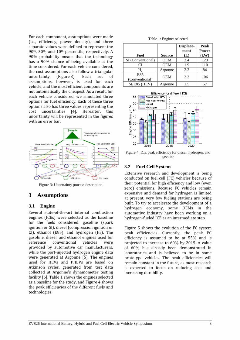
For each component, assumptions were made (i.e., efficiency, power density), and three separate values were defined to represent the 90th, 50th, and 10th percentile, respectively. A 90% probability means that the technology has a 90% chance of being available at the time considered. For each vehicle considered, the cost assumptions also follow a triangular uncertainty (Figure 3). Each set of assumptions, however, is used for each vehicle, and the most efficient components are not automatically the cheapest. As a result, for each vehicle considered, we simulated three options for fuel efficiency. Each of these three options also has three values representing the cost uncertainties [4]. Hereafter, this uncertainty will be represented in the figures with an error bar.

Figure 3: Uncertainty process description

3 Assumptions

3.1 Engine

Several state-of-the-art internal combustion engines (ICEs) were selected as the baseline for the fuels considered: gasoline (spark ignition or SI), diesel (compression ignition or CI), ethanol (E85), and hydrogen (H2). The gasoline, diesel, and ethanol engines used for reference conventional vehicles were provided by automotive car manufacturers, while the port-injected hydrogen engine data were generated at Argonne [5]. The engines used for HEVs and PHEVs are based on Atkinson cycles, generated from test data collected at Argonne’s dynamometer testing facility [6]. Table 1 shows the engines selected as a baseline for the study, and Figure 4 shows the peak efficiencies of the different fuels and technologies.

Table 1: Engines selected

Fuel Source

Displace-

ment

(L)

Peak

Power

(kW)

SI (Conventional) OEM 2.4 123

CI OEM 1.9 110

H2 Argonne 2.2 84

E85

(Conventional) OEM 2.2 106

SI/E85 (HEV) Argonne 1.5 57

Figure 4: ICE peak efficiency for diesel, hydrogen, and

gasoline

3.2 Fuel Cell System

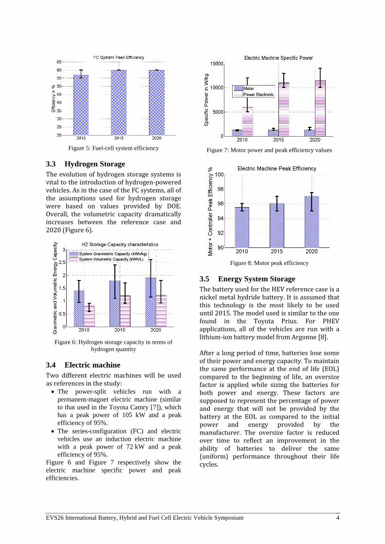
Extensive research and development is being conducted on fuel cell (FC) vehicles because of their potential for high efficiency and low (even zero) emissions. Because FC vehicles remain expensive and demand for hydrogen is limited at present, very few fueling stations are being built. To try to accelerate the development of a hydrogen economy, some OEMs in the automotive industry have been working on a hydrogen-fueled ICE as an intermediate step. Figure 5 shows the evolution of the FC system peak efficiencies. Currently, the peak FC efficiency is assumed to be at 55% and is projected to increase to 60% by 2015. A value of 60% has already been demonstrated in laboratories and is believed to be in some prototype vehicles. The peak efficiencies will remain constant in the future, as most research is expected to focus on reducing cost and increasing durability.


Figure 5: Fuel-cell system efficiency

3.3 Hydrogen Storage

The evolution of hydrogen storage systems is vital to the introduction of hydrogen-powered vehicles. As in the case of the FC systems, all of the assumptions used for hydrogen storage were based on values provided by DOE. Overall, the volumetric capacity dramatically increases between the reference case and 2020 (Figure 6).

Figure 6: Hydrogen storage capacity in terms of

hydrogen quantity

3.4 Electric machine

Two different electric machines will be used as references in the study: The power-split vehicles run with a

permanent-magnet electric machine (similar

to that used in the Toyota Camry [7]), which

has a peak power of 105 kW and a peak

efficiency of 95%.

The series-configuration (FC) and electric

vehicles use an induction electric machine

with a peak power of 72 kW and a peak

efficiency of 95%.

Figure 6 and Figure 7 respectively show the

electric machine specific power and peak

efficiencies.

Figure 7: Motor power and peak efficiency values

Figure 8: Motor peak efficiency

3.5 Energy System Storage

The battery used for the HEV reference case is a nickel metal hydride battery. It is assumed that this technology is the most likely to be used until 2015. The model used is similar to the one found in the Toyota Prius. For PHEV applications, all of the vehicles are run with a lithium-ion battery model from Argonne [8]. After a long period of time, batteries lose some of their power and energy capacity. To maintain the same performance at the end of life (EOL) compared to the beginning of life, an oversize factor is applied while sizing the batteries for both power and energy. These factors are supposed to represent the percentage of power and energy that will not be provided by the battery at the EOL as compared to the initial power and energy provided by the manufacturer. The oversize factor is reduced over time to reflect an improvement in the ability of batteries to deliver the same (uniform) performance throughout their life cycles.


Table 2: Battery Technologies

Figure 9res 9 and 10 show battery cost. The

battery cost for HEV applications will decrease

over time for all cases, but the reduction is more

aggressive for the high case between 2010 and

2015.

Figure 9: HEV battery cost

Figure 10: PHEV and EV battery cost

3.6 Vehicle

One of the main factors affecting fuel

consumption is vehicle weight. Lowering the

weight (“light-weighting”) reduces the forces

required to follow the vehicle speed trace. As a

result, the components can be downsized,

resulting in decreased fuel consumption. However, the impact of lightweighting is not the

same for all of the powertrain configurations;

studies have shown that the technology has greater

influence in lowering fuel consumption in

conventional vehicles than it does in their electric-

drive counterparts [9] (Figure 11).

Glider

Mass

(kg)

Frontal

Area

(m2)

Tire

Wheel

Radius

(m)

Midsize 996 2.24 P195/65/R15 0.317

Figure 11: Glider mass reduction

Reductions in rolling resistance, frontal area, and

drag coefficient also have the potential to improve

fuel consumption significantly, as these factors

also lead to a reduction in the force required at the

wheels.

4 Vehicle Technical Specifications

All of the vehicles have been sized to meet the same requirements: Initial vehicle movement to 60 mi/h in 9 sec

+/− 0.1 sec,

Maximum grade of 6% at 65 mi/h at gross

vehicle weight, and

Maximum vehicle speed >100 mi/h.

These requirements are a good representation of the current American automotive market as well as American drivers’ expectations.


Table 3 summarizes the travel distances with a full tank of fuel for the different powertrains. The vehicles using gasoline, diesel, or ethanol fuel have been sized for a distance of 500 miles on the combined driving cycle, based on unadjusted fuel consumption. All vehicles have a range of at least 320 miles except the battery electric vehicle (BEV) (100 miles) and the hydrogen vehicles.

Table 3: Travel distances in miles

Time frame

Vehicle

Type Ref 2010 2015 2020

Conv. H2 320 320 320 320

HEV H2,

FC 320 320 320 320

PHEV H2,

FC

320 +

AERa

320 +

AER

320 +

AER

320 +

AER

BEV 100 100 100 100

a AER = all-electric range.

Input mode power-split configurations, similar to

those used in the Toyota Camry, were selected

for all HEV and PHEV applications using

engines. The series FC configurations use a two-

gear transmission to be able to achieve the

maximum vehicle speed requirement. The

vehicle-level control strategies employed for

each configuration have been defined in previous

publications [10-15].

5 Vehicle Sizing Several automated sizing algorithms were

developed to provide a fair comparison between

technologies. These algorithms are specific to the

powertrain (i.e., conventional, power-split, series,

electric) and the application (i.e., HEV, PHEV).

As shown in Figure 12, the engine power for all

of the powertrains decreases over time. The

power-split HEV powertrain shows the highest

engine power reduction, ranging from 6% to

36%, whereas power for the conventional engine

decreases by only 3% to 27%. The engine power

is higher when the all-electric range increases

because the power is sized on the basis of

acceleration and grade and because the different

PHEVs (for the same fuel) vary from one another

only by having a successively larger battery

(which results in a heavier car).

Figure 12: Engine power for gasoline-fueled cars

Figure 13 shows the electric machine power for the

gasoline HEVs and PHEVs. The electric machines

used for the PHEV10 and PHEV20 cases are sized

to have the ability to follow the UDDS drive cycle

in EV mode, while those used for the PHEV30 and

PHEV40 cases allow the vehicles to follow the

US06 drive cycle. It is important to note that the

vehicles have the ability to drive the UDDS cycle

in electric mode—the control strategy employed

during fuel-efficiency simulation—which is based

on blended operation. However, the power does

not increase significantly compared to HEVs for

the power-split configuration.

Figure 13: Motor power for hybrid cars

6 Vehicle Simulation Results

The vehicles were simulated on both the UDDS and HWFET drive cycles. The cold-start penalties shown in Table 4 were defined for each powertrain technology option on the basis of available data collected at Argonne’s dynamometer facility and available in the literature. This percentage is the penalty applied after simulation to the fuel economy value, since all simulations run under hot conditions.


Table 4: Cold-start penalty values

Powertrain 2010 2015 2020

Conventional 12%

15

15

15

15

15

15

15

15

15

15

15

15

Power-Split HEV 8%

18

18

18

18

18

18

18

18

18

18

18

18

Power-Split PHEV 6%

14

14

14

14

14

14

14

14

14

14

14

14

FC HEV 0%

25

25

25

25

25

25

25

25

25

25

25

25

FC PHEV 0%

15

15

15

15

15

15

15

15

15

15

15

15

Electric 5%

10

10

10

10

10

10

10

10

10

10

10

10

Figure 14 shows fuel consumption results for a midsize car, focusing on different gasoline-fueled configurations.

Figure 14: Fuel consumption for midsize cars with

various gasoline-fueled configurations

As shown in Table 5 and Table 6, the comparisons between power-split HEVs and conventional gasoline engines show that the percentage improvement ranges around 15.9% for conventional, whereas it ranges from 4% to 23% for HEVs. This shows that HEV vehicles are more sensitive to the uncertainty. PHEVs range similarly to HEVs, with a large discrepancy shown (3%-29% for PHEV10, 3-20% for PHEV 30).

Table 5: Fuel consumption for vehicles with ICE (low

uncertainty)

Low uncertainty

2010 2020 Improvement

Conventional 5.16 4.34 15.9%

HEV 3.87 2.97 23.3%

Split PHEV10 3.24 2.29 29.3%

Split PHEV20 2.19 1.88 14.2%

EREV

PHEV30 2.05 1.62 21.0%

EREV

PHEV40 1.75 1.36 22.3%

Note that PHEV10 vehicles will benefit more from advances in the future for the low case scenario, whereas conventional vehicles show a 15% improvement in the high case scenario.

Table 6: Fuel consumption for vehicles with ICE (high

uncertainty)

High uncertainty


Conventional 7.21 6.06 15.95%

HEV 4.72 4.5 4.7%

Split PHEV10 3.54 3.42 3.4%

Split PHEV20 2.68 2.57 4.1%

EREV PHEV30 2.44 2.35 3.7%

EREV PHEV40 2.07 1.98 4.3%

Figure 15 shows fuel consumption results for midsize cars, focusing on FC vehicles.

Figure 15: Fuel consumption for midsize fuel-cell cars

As shown in Table 7 and table 8, the fuel cell (FC) PHEV10 consumes around 15% less in 2020 for both low and high cases. Other FC vehicles shows fuel consumption improvements ranging from 5% to 14%

Table 7: Fuel consumption for fuel cell vehicles (low

uncertainty)

Low uncertainty


FC PHEV10 2.18 1.87 14.2%

FC PHEV20 1.96 1.67 14.8%

FC PHEV30 1.37 1.3 5.1%

FC PHEV40 1.15 1.07 7.0%

Table 8: Fuel consumption for fuel cell vehicles (low

uncertainty)

High uncertainty


FC PHEV10 3.1 2.62 15.5%

FC PHEV20 2.52 2.36 6.3%

FC PHEV30 1.88 1.61 14.4%

FC PHEV40 1.58 1.35 14.6%


Note that fuel cell vehicle technology will

continue to provide less fuel efficiency

improvement than the technologies for the

gasoline HEVs as well as conventional gasoline

engines.

Figure 16 shows the electric consumption for a

BEV on the UDDS and HWFET cycles. No

significant difference in electrical consumption is

observed between the two cycles. The main

reason is that the electric machine operates at

high efficiency points at both low and high

speeds. Nevertheless, electric consumption

decreases slightly over time between 2010 and

2020. This decrease is due to the small

improvement in the electric machine efficiency

and lightweighting.

Figure 16: Electric consumption for midsize BEV

Figure 17 shows the incremental cost versus fuel

consumption for gasoline vehicles. Incremental

cost compares actual cost to the baseline (2010)

conventional gasoline engine. Note that vehicles

at the bottom right are the most cost-effective

(low cost, low fuel consumption). It is hard to

draw a conclusion, but it can be said that

PHEV40 vehicles are significantly cheaper and

more efficient in 2020 than in 2010, whereas

conventional-vehicle cost remains constant over

those years.

0.511.522.533.5

0

1

2

3

4x 10

4

Fuel Consumption (gallons/100mile)

Cost ($

)

2010

2010

2015

2020

2030

2045

Dark Blue = Conv

Green = Split HEV

Yellow = Split PHEV10

Red = Split PHEV20

Light Blue = Erev PHEV30

Black = Erev PHEV40

Figure 17: Incremental cost vs. fuel consumption for

gasoline-fueled midsize cars.

Figure 18 shows the incremental cost versus fuel

consumption for FC vehicles. The cost spread

between 2010 and 2020 is higher for the FC

PHEV40 than for the other FC vehicles; i.e., the

FC PHEV40 is more likely to show improvement

over those years. Note that in 2020 the cost

differential among FC PHEV vehicles is small,

especially for FC PHEV10 vs. FC PHEV20 and

FC PHEV30 vs. FC PHEV40.

00.511.520

1

2

3

4

5x 10

4

Fuel Consumption (gallons/100mile)

Cost ($

)

2010

2015

2020

Dark Blue = FC HEV

Green = FC PHEV10

Yellow = FC PHEV20

Red = FC PHEV30

Light Blue = FC PHEV40

Figure 18: Incremental cost vs. fuel consumption for

midsize fuel-cell cars

7 Market Penetration

Assessing the fuel displacement potential of

specific technology platforms on a national scale

requires an analysis of their market penetration

potential. One approach to do so is to compare the

lifecycle vehicle cost (the sum of initial vehicle

cost plus the net present value of fuel costs over

the vehicle’s lifetime, expressed as cents/mile)

across technology platforms to examine whether

incremental costs for advanced technology

vehicles are sufficiently counterbalanced by

reduced operating costs such that the market is

willing to accept those advanced vehicles. A

prerequisite step to summing vehicle and fuel costs

is a method for aligning the timing of payments: a

vehicle purchase payment is assumed to be made

only once at the beginning of a vehicle’s life (note

that financing the vehicle into a series of payments

over time would change this calculation) but fuel

purchases are made regularly over the life of the

vehicle. This analysis uses a net present value of

the sum of annual fuel expenditure (discounted at

7%) to estimate the value of the total expected


expenditure on fuel at the point of vehicle

purchase:

NPV =$

gal·VMT

mpg·

1

(1+d)tt=1

15

å (1)

The above equation calculates the net present

value (NPV) of fuel as the product of the price of

fuel ($/gal), the amount of fuel purchased

annually (10,000 average vehicle miles travelled

per year, VMT, divided by fuel economy, mpg,

which is a function of the vehicle architecture

modelled in Autonomie), and a coefficient to

reflect the discounted (at d = 7%) cash flow over

a vehicle lifetime of 15 years. For each

powertrain modelled, the net present value of

fuel is added directly to the estimated vehicle

purchase price to arrive at vehicle lifecycle costs,

which are presented for all advanced powertrains

as a percentage of the lifecycle cost of the

Reference SI vehicle described in the preceding

modelling sections in Figure 19. Specifically,

Figure 19 compares the lifecycle costs for

advanced powertrains in the Low- and High-

Tech scenarios in 2010 and 2020 to illustrate

how lifecycle costs for advanced vehicles are

expected to decline over time, and, to draw

attention to the extent to which a High-Tech

case, in which advanced technologies achieve

higher performances and lower costs, can lower

the lifecycle cost of advanced technology

vehicles to a level below that of a conventional

Reference vehicle by 2020. Note that in the

High-Tech scenario, all advanced powertrains

cost less than 100% of the Reference SI vehicle’s

lifecycle cost by 2020. In the Low-Tech

scenario, advanced powertrains still require

performance advances and/or cost reductions to

achieve Reference SI-comparable lifecycle costs.

Figure 19 - Lifecycle cost comparison in 2010 and

2020 in High- and Low-tech scenarios

An advanced vehicle achieving a vehicle lifecycle

cost less than that of a Reference SI vehicle is not

sufficiency to guarantee the market update of that

vehicle. The ratio of incremental vehicle cost and

annual fuel savings is a critical factor in

determining the period over which an advanced

technology vehicle’s fuel savings will offset initial

incremental price. Figure 20 depicts lifecycle

costs at the 50% level (with the 10% and 90%

shown as lower and upper bounds, respectively)

decomposed into vehicle component capital costs

and fuel costs to facilitates an examination of how

advanced component technologies (which

contribute to initial vehicle cost) and overall

vehicle efficiency (which reduce fuel cost)

contribute to total cost of ownership. Note that

higher levels of electrification are associated with

higher initial vehicle costs, lower fuel cost, and

higher technology uncertainty (the range of

possible lifecycle costs for each technology

platform). Note that, for example, the advanced SI

vehicle in 2010 costs slightly more than the

Reference vehicle, suggesting that the decrease in

fuel expenditure achieved by that powertrain does

not fully offset the incremental price of the

vehicle, and likewise for other advanced

powertrains. The PHEV40 and EV architectures

stand out as especially expensive, despite very low

fuel costs, which is not surprising given the high

present-day costs associated with relatively large

batteries these powertrains incur. By 2020, all

initial vehicle costs decline as a result of expected

technology improvement (as noted in preceding

modelling discussions). Fuel costs, conversely,

increase, despite an increase in efficiency for all

powertrains (also noted in preceding modelling

discussions), as a result of an increase in fuel

prices over time [16]. The very high efficiency of

electric-drive vehicles combined with a smaller

increase in electricity prices relative to the increase

in petroleum-product prices, results in a far smaller

change in fuel cost for the PHEV40 and EV. The

fuel cell vehicle fuel costs decrease as a result of

an assumption that DOE H2 fuel cost goals are met

by 2020 [17]. Note that Figure 20 is consistent

with Figure 19 with respect to which powertrains

achieve Reference SI-comparable lifecycle costs

by 2020 at the 10% levels (indicated by the lower

bound of the uncertainty bands).


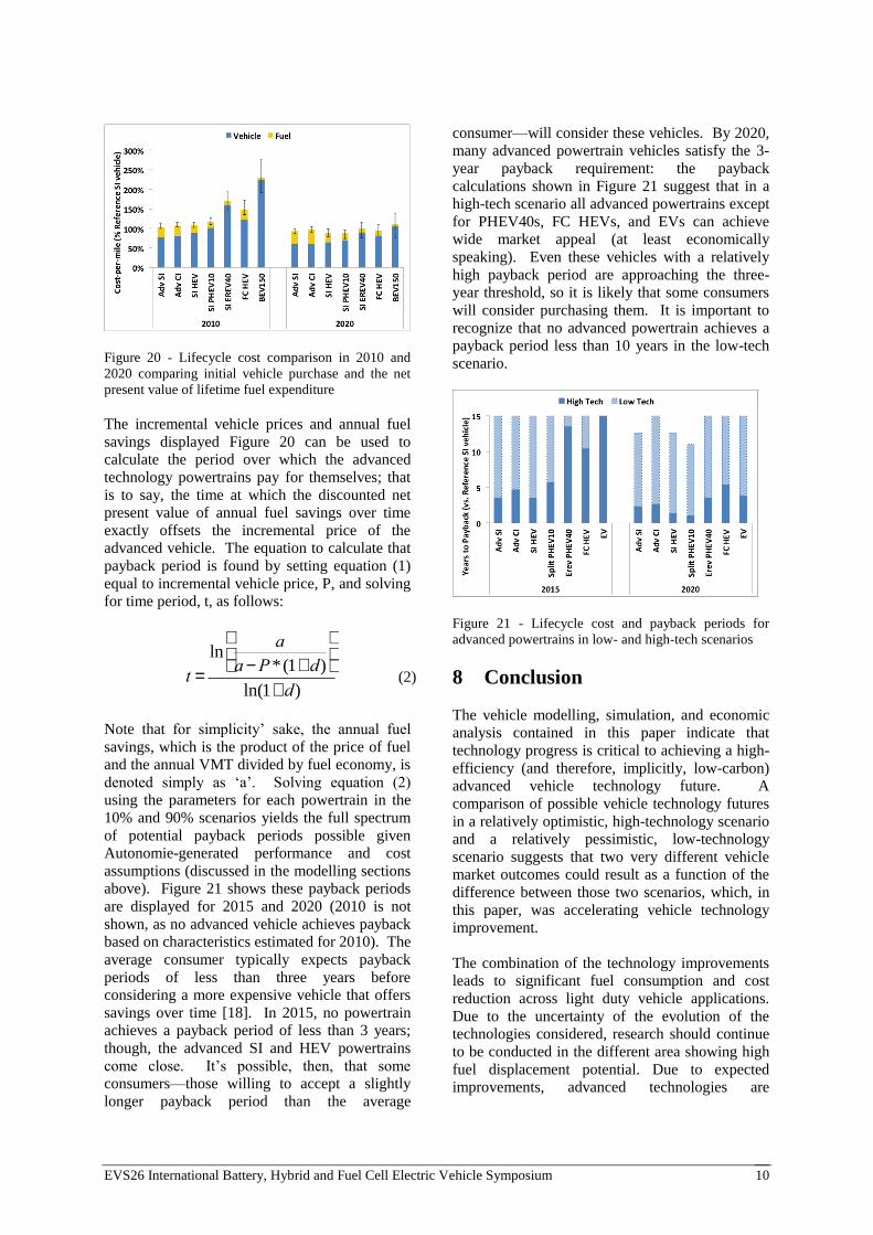
Figure 20 - Lifecycle cost comparison in 2010 and

2020 comparing initial vehicle purchase and the net

present value of lifetime fuel expenditure

The incremental vehicle prices and annual fuel

savings displayed Figure 20 can be used to

calculate the period over which the advanced

technology powertrains pay for themselves; that

is to say, the time at which the discounted net

present value of annual fuel savings over time

exactly offsets the incremental price of the

advanced vehicle. The equation to calculate that

payback period is found by setting equation (1)

equal to incremental vehicle price, P, and solving

for time period, t, as follows:

t =

lna

a-P*(1+ d)

æ

èç

ö

ø÷

ln(1+ d) (2)

Note that for simplicity’ sake, the annual fuel

savings, which is the product of the price of fuel

and the annual VMT divided by fuel economy, is

denoted simply as ‘a’. Solving equation (2)

using the parameters for each powertrain in the

10% and 90% scenarios yields the full spectrum

of potential payback periods possible given

Autonomie-generated performance and cost

assumptions (discussed in the modelling sections

above). Figure 21 shows these payback periods

are displayed for 2015 and 2020 (2010 is not

shown, as no advanced vehicle achieves payback

based on characteristics estimated for 2010). The

average consumer typically expects payback

periods of less than three years before

considering a more expensive vehicle that offers

savings over time [18]. In 2015, no powertrain

achieves a payback period of less than 3 years;

though, the advanced SI and HEV powertrains

come close. It’s possible, then, that some consumers—those willing to accept a slightly

longer payback period than the average

consumer—will consider these vehicles. By 2020,

many advanced powertrain vehicles satisfy the 3-

year payback requirement: the payback

calculations shown in Figure 21 suggest that in a

high-tech scenario all advanced powertrains except

for PHEV40s, FC HEVs, and EVs can achieve

wide market appeal (at least economically

speaking). Even these vehicles with a relatively

high payback period are approaching the three-

year threshold, so it is likely that some consumers

will consider purchasing them. It is important to

recognize that no advanced powertrain achieves a

payback period less than 10 years in the low-tech

scenario.

Figure 21 - Lifecycle cost and payback periods for

advanced powertrains in low- and high-tech scenarios

8 Conclusion

The vehicle modelling, simulation, and economic

analysis contained in this paper indicate that

technology progress is critical to achieving a high-

efficiency (and therefore, implicitly, low-carbon)

advanced vehicle technology future. A

comparison of possible vehicle technology futures

in a relatively optimistic, high-technology scenario

and a relatively pessimistic, low-technology

scenario suggests that two very different vehicle

market outcomes could result as a function of the

difference between those two scenarios, which, in

this paper, was accelerating vehicle technology

improvement.

The combination of the technology improvements

leads to significant fuel consumption and cost

reduction across light duty vehicle applications.

Due to the uncertainty of the evolution of the

technologies considered, research should continue

to be conducted in the different area showing high

fuel displacement potential. Due to expected improvements, advanced technologies are


expected to have significant market penetration

over the next decades. In the short term, both

engine HEVs and PHEVs allow for significant

fuel displacement with acceptable additional

cost. While electric vehicles do provide a

promising solution, they are likely to remain

expensive and range limited in the near future.

Acknowledgments This study was supported by the DOE Vehicle

Technologies Office. The submitted report has

been created by UChicago Argonne, LLC,

Operator of Argonne National Laboratory

(Argonne). Argonne, a DOE Office of Science

laboratory, is operated under Contract No. DE-

AC02-06CH11357. The U.S. Government retains

for itself, and others acting on its behalf, a paid-

up, nonexclusive, irrevocable worldwide license

in said article to reproduce, prepare derivative

works, distribute copies to the public, and

perform publicly and display publicly, by or on

behalf of the Government.

References [1] Available at

http://www1.eere.energy.gov/ba/

pba/program_benefits.html.

[2] Available at http://www.autonomie.net/

overview/papers_software.html.

[3] Moawad, A., P. Sharer, and A. Rousseau

(2011). Light-Duty Vehicle Fuel

Consumption Displacement Potential up to

2045. Available at

http://www.autonomie.net/publications/fuel

_economy_report.html

[4] Henrion, M. (2008). Guide to Estimating

Unbiased Probability Distributions for

Energy R&D Results. DOE Risk Analysis

Group.

[5] Wallner, T., and H. Lohse-Busch (2007).

Performance, Efficiency, and Emissions

Evaluation of a Supercharged, Hydrogen-

Powered, 4-Cylinder Engine. SAE paper

2007-01-0016, presented at the SAE Fuels

and Emissions Conference, Capetown,

South Africa, January. Available at

http://papers.sae.org/2007-01-0016.

[6] Bohn, T.A. (2005). Implementation of a

Non-Intrusive In-Vehicle Engine Torque

Sensor for Benchmarking the Toyota Prius

HEV. SAE paper 2005-01-1046, presented

at the SAE World Congress & Exhibition,

Detroit, Mich., April.

[7] Olszewski, M. (2008). Evaluation of the 2007

Toyota Camry Hybrid Synergy Drive System.

Report for the U.S. Department of Energy,

January. Available at

http://www.osti.gov/bridge/servlets/purl/9286

84-rRNS3c/928684.pdf

[8] Sharer, P., A. Rousseau, P. Nelson, and S.

Pagerit (2006). Vehicle Simulation Results for

PHEV Battery Requirements. 22nd

International Electric Vehicle Symposium

(EVS22), Yokohama, October.

[9] Pagerit, S., P. Sharer, and A. Rousseau

(2006). Fuel Economy Sensitivity to Vehicle

Mass for Advanced Vehicle Powertrains.

SAE paper 2006-01-0665, presented at the

SAE World Congress & Exhibition, Detroit,

Mich., April.

[10] Freyermuth, V., E. Fallas, and A. Rousseau

(2008). Comparison of Powertrain

Configuration for Plug-in HEVs from a Fuel

Economy Perspective. SAE paper 2008-01-

0461, SAE World Congress, Detroit, Mich.,

April.

[11] Rousseau, A., P. Sharer, S. Pagerit, and M.

Duoba (2006). Integrating Data, Performing

Quality Assurance, and Validating the

Vehicle Model for the 2004 Prius Using

PSAT. SAE paper 2006-01-0667, SAE World

Congress, Detroit, Mich., April.

[12] Pagerit, S., A. Rousseau, and P. Sharer

(2005). Global Optimization to Real Time

Control of HEV Power Flow: Example of a

Fuel Cell Hybrid Vehicle. 20th International

Electric Vehicle Symposium (EVS20),

Monaco, April.

[13] Sharer, P., A. Rousseau, D. Karbowski, and

S. Pagerit (2008). Plug-in Hybrid Electric

Vehicle Control Strategy: Comparison

between EV and Charge-Depleting Options.

SAE paper 2008-01-0460, SAE World

Congress, Detroit, Mich., April.

[14] Cao, Q., S. Pagerit, R. Carlson, and A.

Rousseau (2007). PHEV Hymotion Prius

Model Validation and Control Improvements.

23rd International Electric Vehicle

Symposium (EVS23), Anaheim, Calif.,

December.

[15] Karbowski, D., A. Rousseau, S. Pagerit, and

P. Sharer (2006). Plug-in Vehicle Control

Strategy: From Global Optimization to Real

Time Application. 22nd International Electric

Vehicle Symposium (EVS22), Yokohama,

Japan, October.

[16] Energy Information Administration, Annual

Energy Outlook 2011, at:

http://www.eia.gov/forecasts/archive/aeo11/

http://www.autonomie.net/publications/fuel


[17] U.S. Department of Energy Fuel Cell

Technologies Program, Hydrogen

Threshold Cost Calculation, at:

www.hydrogen.energy.gov/pdfs/11007_h2_

threshold_costs.pdf

[18] Greene, D. (2007), Testimony to the United

States Senate Committee on Environment

and Public Works, November 13.

Authors

Jacob Ward

Senior Analyst

U.S. Department of Energy,

1000 Independence Ave, SW,

Washington, DC 20585, USA

Tel: +1-202-586-7606

Email: [email protected]

Jacob Ward is the Lead Analyst for the

Vehicle Technologies Program at the

U.S. Department of Energy’s Office of

Energy Efficiency and Renewable

Energy. Jake joined the DOE in 2008

as a Presidential Management Fellow

after earning a Master of Public Policy

from Georgetown University; he also

holds a BS in Mechanical Engineering

and a BA in Latin American Studies

from the University of Texas at

Austin. He received the Secretary’s

Appreciation Award in 2010 for his

work interpreting the long-term

benefits of American Reinvestment

and Recovery Act projects.

Ayman Moawad

Research Engineer

Argonne National Laboratory,

9700 S. Cass Avenue,

Lemont, IL 60439, USA

Tel: +1-630-252-2849


Ayman Moawad is a research engineer

in the Vehicle Modeling and

Simulation Section at Argonne

National Laboratory. He graduated

from the Ecole des Mines de Nantes,

France, in 2009 with a Master’s

Degree in Science, majoring in

Automatics, Control Systems, and

Industrial Computer Science. He

focuses his research on light-duty

vehicle fuel-consumption analysis, as

well as powertrain costs, to support the

Government Performance and Results

Act.

Namdoo Kim

Research Engineer




Tel: +1-630-252-2843


Namdoo Kim graduated in 2007 from

the University of Sungkyunkwan,

Korea, with a Master’s degree in the

School of Mechanical Engineering. He

is currently working in Argonne

National Laboratory’s Vehicle

Modeling and Simulation Group.

Aymeric Rousseau

Program Manager




Tel: +1-630-252-7261


Aymeric Rousseau is the Manager of

the Vehicle Modeling and Simulation

Section at Argonne National

Laboratory. He received his

engineering diploma at the Industrial

System Engineering School in La

Rochelle, France, in 1997. After

working for PSA Peugeot Citroen in

the Hybrid Electric Vehicle research

department, he joined Argonne

National Laboratory in 1999, where he

is now responsible for the

development of Autonomie. He

received an R&D100 Award in 2004

and a 2010 Vehicle Technologies

Program R&D Award in 2010. He has

authored more than 40 technical

papers in the area of advanced vehicle

technologies.

mailto:[email protected]




Date post:	07-Feb-2018
Category:	Documents
Upload:	vutram
View:	218 times
Download:	3 times

Light-duty-vehicle fuel consumption, cost and market ... - Papers/Light duty/JW - EVS26.pdf ·...

Documents