Limited Arbitrage Analysis of CDS-Basis...

Limited Arbitrage Analysis of CDS-Basis Trading

Qi SHANG∗ [email protected]

First version: Dec 2009 This version: Nov 2011

Abstract

By modeling time-varying funding costs and demand pressure as the limits to arbitrage, thepaper shows that assets with identical cash-flows have not only different expected returns,but also different expected returns in excess of funding costs. I solve the model in closed-form to show that arbitrage on the CDS and corporate bond market is risky regardless ofthe degree of price discrepancy. The profitability and risk of this arbitrage, which is calledCDS-basis trading, are increasing in market friction levels and assets’ maturities. High levelsof market frictions also destruct the positive predictability of credit spread term structureon credit spread changes. Empirical results support model predictions. CDS-basis tradingis exposed to systematic risk factors, while TED spread squared times adjusted corporatebond trading volume predicts abnormal CDS-basis trading return in the latter half of 2008.

∗Webpage: http://personal.lse.ac.uk/shang I owe special thanks to Dimitri Vayanos and Kathy Yuan fortheir many comments and suggestions. Also, I am very grateful to Mikhail Chernov, Amil Dasgupta, DanielFerreira, Stephane Guibaud, Shiyang Huang, Dong Lou, Philippe Mueller, Christopher Polk, Zhigang Qiu,Michela Verardo, Jean-Pierre Zigrand and seminar participants at the LSE/FMG PhD Seminar for manyhelpful suggestions. All remaining errors are my own.

1

1 Introduction

As summarized in Gromb and Vayanos (2010), costs or demand shocks faced by arbitrageurscan prevent them from eliminating mis-pricings on the markets and therefore generate mar-ket anomalies. My model illustrate how the interaction of time-varying funding cost anddemand pressure faced by arbitrageurs results in two assets with identical payoffs havingdifferent expected excess return. This result imply taking opposite positions on these twoassets is a risky arbitrage that is expected to earn profit in excess of funding costs. I thenuse CDS basis trading, which is the arbitrage using CDS and corporate bonds, as an exam-ple to derive implications of the model and find supportive empirical evidence.

I explain the riskiness of arbitraging on two defaultable bonds with identical cash-flows asthe result of the interaction of funding illiquidity and market illiquidity. Under a continuous-time demand-based framework in which risk-averse arbitrageurs trade on two markets withidentical defaultable bonds to meet demand pressure posed by local investors, the pres-ence of demand pressure results in arbitrageurs requiring risk premium for the positionsthey take. Without other frictions, demand pressure alone doesn’t generate pricing dis-crepancies between assets with identical cash-flows. Arbitrageurs also face time-varyingfunding costs on the two markets, which under certain conditions result in the two assetshave different risk exposures and carry different levels of risk premium. The co-existence oftime-varying funding cost and demand pressure makes taking opposite positions on the twomarkets a risky arbitrage. As shown in the model, without any one of these two sources offriction, the arbitrage doesn’t generate expected excess profit.

I solve the model in closed-form under two cases. The first case assumes constant demandpressures from local investors while the second case assumes opposite stochastic demandpressures. In the latter case, even if the arbitrageurs can take the exact opposite positionson the two markets in equilibrium so that they are completely protected from the risk ofdefaults, they still have non-zero exposures to other risk factors. Applying the results to theCDS and corporate bond markets suggests CDS basis trading is in fact risky arbitrage andit is reasonable for the CDS basis to deviate from its theoretical frictionless value of zerounder severe market frictions. The profitability of the risky arbitrage depends on marketfrictions rather than the level of the price discrepancy. The model also shows the arbi-trageurs sometimes magnify rather than correct price distortion under market frictions andoffers a number of results on term structure properties.

Empirical results support the model predictions. Using Markit CDX and iBoxx Indicesdata and corporate bond data from TRACE, I show that basis trading is exposed to system-atic risk factors, while the interaction of funding cost and market liquidity have predictivepower on abnormal basis trading returns. As predicted by the model, the predictability ofcredit spread term structure slope on future credit spread change disappears when marketfrictions are high. I also find the size and volatility of realized basis trading excess return

2

is increasing in the degree of market frictions. Moreover, basis trading profit is increasingin underlying maturity and the size of CDS basis is increasing in corporate bond markettrading volume.

In early theoretical literature, Tuckman and Vila (1990) show that exogenous price dis-crepancies between two assets with identical cash-flows do not necessarily create arbitrageopportunities if there’s shorting-selling cost. As show in Gromb and Vayanos (2010), with-out other frictions, the discrepancies between the expected returns of the two assets shouldcompensate exactly for the funding costs so that an arbitrageur is still expected to earnzero excess return. In contrary, my model suggests arbitrageur can earn a risky profit evenafter adjusting for the funding costs if the funding costs are time-varying and arbitrageurfaces demand pressure.

The demand pressure faced by the arbitrageurs is another important source of market fric-tion that contributes to the rise of market anomalies. Investors other than arbitrageurs canhave endogenous demand shocks that arise via different channels,1 but a number of papershave focused on the pricing implications given exogenous demand shocks as I do. These the-oretical demand-based papers include Garleanu, et.al.(2009), Naranjo (2009) and Vayanosand Villa (2009). By assuming exogenous underlying asset prices, Garleanu, et.al.(2009)and Naranjo (2009) solve derivative prices endogenously to show that exogenous demandshocks and frictions in arbitrageurs’ trading can drive derivative prices away from conven-tional prices implied by the no-arbitrage conditions. Naranjo (2009) considers extra fundingcost faced by arbitrageurs as the friction limiting her ability to eliminate price discrepancieson the futures and underlying markets. However, he assumed the underlying asset’s price asexogenously given, so the market frictions only have impact on the futures price but not onthe underlying market, which is unrealistic as derivative markets’ trading do have impacton underlying price.

My paper is the closest to Vayanos and Vila (2009) in that prices on all markets are endoge-nized so frictions on one market affect all markets. Vayanos and Villa (2009) study arbitrageacross different Treasury bonds maturities, i.e. assets with different cash-flows, and there’sno other frictions than the demand shocks from other preferred habitat investors. However,my paper introduces an additional friction, which is the time-varying funding costs, to showthat two assets with identical cash-flows can earn different expected excess return, whichimplies profitability yet risk for a cross-market arbitrage trade. The two assets with iden-tical cash-flows are two defaultable bonds, one represents corporate bond, while the otherrepresents a synthetic corporate bond position created by writing a CDS protection anddefault-free lending.2 Trading corporate bonds through repo and reverse-repo generates ad-ditional funding costs that are sensitive to default intensity of the bonds. Therefore I model

1See Gromb and Vayanos (2010) for details.2The equivalence of synthetic corporate bond and writing CDS plus lending will be illustrated in the next

section.

3

the funding costs as functions of default intensity. Although the assumption on fundingcosts are not fully endogenized, a clear motivation in Appendix A along with empiricalfindings by Gorton and Metrick (2010) justify this assumption, which is further supportedby a recent paper by Mitchell and Pulvino (2011), which illustrates the consequence offunding liquidity failure on arbitrage activities from practitioners’ perspectives.

I apply the model’s implications on CDS basis trading, which turned out to be a riskyarbitrage activity in the 2007/08 crisis. Credit default swap (CDS) is an OTC contract inwhich one party pays the other party a periodical fee (the CDS premium) for the protectionagainst credit events of an underlying bond, in which case the protection seller pays theprotection buyer for the loss from the underlying bond. The CDS market offers hedgers andspeculators to trade credit risks in a relatively easy way. It is a fast growing market withvast market volume. The exact way to trade CDS has experienced some significant changesin the recent years following hot debates over the role it plays in the 2007/08 financial crisis.In the past, the two parties of a CDS trade agree on the CDS premium that makes theCDS contract having zero value at origination. Then as conditions change in the life of thiscontract, it has a marked-to-market value that is not zero. Following the implementationof the so-called CDS Big-Bang regulations on the North American markets in April 2009,the CDS premia are fixed at either 100bps or 500bps, and the two parties exchange anamount of cash at origination to reflect the true value of the contract. For instance, if thereasonable CDS premium should be 200bps, then the protection buyer pays the protectionwriter a certain amount of money at the beginning, and then pays CDS premium at 100bpseach period. This is certainly a change in order to make the market more standardized andmore liquid, however, the CDS market is still very opaque and illiquid.

Theoretical papers such as Duffie (1999) and Hull and White (2000) show the parity be-tween CDS price and credit spread under the no-arbitrage condition, i.e. investors who holda defaultable bond and short a CDS (buy protection) on this bond is effectively holding adefault-free bond and thus should earn the risk free return. In other words, the CDS basis,which is CDS premium minus the credit spread, should be zero if basis trading earns onlyrisk free return. Empirical works including Hull, et. al.(2004), Blanco, et. al.(2005) and Zhu(2006) using relatively early data support this zero basis hypothesis. However, practitionersobserve positive or negative basis at times and many investors engage in basis trading. Buy-ing a bond and CDS protection is known as negative basis trading, while shorting a bondand writing CDS protection is called positive basis trading. Meanwhile, recent work byGarleanu and Pedersen (2009) and Fontana (2010) document large negative basis persistedfrom the summer of 2007 to early 2009. Figure 1 shows that during the 2007/08 crisis theCDS basis become very negative for a long period, which contradicts text-book arbitrageargument, yet negative basis trading still lost money even at quite negative CDS basis level.In this paper, I reveal the risky arbitrage nature of CDS basis trading in closed-form andshow the profitability of basis trading depends on market frictions rather than the level ofCDS basis.

4

To justify the deviation from the law of one price on the CDS and corporate bond markets,Garleanu and Pedersen (2009) attributes two otherwise identical assets’ different exposuresto risk factors to the different level of exogenous margin requirement on the two markets.Empirical work by Fontana (2010) found that funding costs variables are important in ex-plaining CDS basis changes, while Bai and Collin-Dufresne (2010) explained cross-sectionalvariations in CDS basis with funding liquidity risk, counterparty risk and collateral quality.However, their results concerned only on the changes in CDS basis, which according to mymodel doesn’t determine the profitability of basis trading in the presence of funding costs.My paper is also related to a number of empirical works in explaining credit spread andCDS price movements such as: Collin-Dufresne, et. al.(2001), Elton, et. al.(2001), Huangand Huang (2003), Blanco, et. al.(2005), Tang and Yan (2007), and Ellul, et. al.(2009)among others. A recent work of Giglio (2011) proposed a novel way of inferring impliedjoint distribution of financial institution’s default risk from the CDS basis, which shows therole of counterparty risk in widening CDS basis.

The next section introduces model set-up while Section 3 solves the model under two casesand provides a number of results on the expected excess return of basis trading and the termstructure properties of credit spread and basis trading profits. I then carry out empiricalstudy in Section 4 to verify theoretical results. Finally, Section 5 concludes the paper.

2 The Model

2.1 The Markets

In a continuous time economy with a horizon from zero to infinity, there are two defaultablebond markets C and D, each with a continuum of zero-coupon3 defaultable bonds with facevalue of one and time to maturity τ , τ ∈ (0, T ]. Denote the time t prices of these bondsby P c

t (τ) and P dt (τ) respectively. Assume all bonds on the two markets are issued by the

same entity, so that a bond on market C has identical cash-flow as the bond on market Dwith the same time to maturity. Therefore, the model is in line with other limited-arbitragemodels in deriving price discrepancies between assets with identical cash-flows under mar-ket frictions. When applying equilibrium results to explain real world phenomenon, I referto bond market C as the cash market, which corresponds to the corporate bond market,and bond market D as the derivative market, which corresponds to the CDS market plusdefault-free lending. The linkage between synthetic defaultable bond position and CDS plusdefault-free lending is given at the end of this sub-section.

Upon the exogenous default of the underlying entity, the bond holder loses L fractionof the bond’s market value. To keep the model tractable, I assume L is constant. Nowsuppose Nt is the counting process for the underlying bond’s default time T ′, which is a

3The coupon rate is assumed to be zero so as to derive closed form solutions.

5

doubly-stochastic stopping time4. Nt = 0 if no default happens before time t and Nt = 1if default happens before time t. Here, I model Nt as a counting process with a intensityλ+ λt. In general:

Nt =∫ t

0(λ+ λs)ds+Mt (1)

where Mt is a jump martingale that jumps to one at the time of default. The stochastic λt

follows the Ornstein-Uhlenbeck process:

dλt = κλ(λ− λt)dt+ σλdBλ,t (2)

I also assume that the money invested into money market account generates instantaneousreturn at an exogenous short rate rt, which also follows an Ornstein-Uhlenbeck process:

drt = κr(r − rt)dt+ σrdBr,t (3)

In early literature such as Duffie (1999), the equivalence of defaultable bond and CDS plusdefault-free lending is best illustrated in the case of floating rate notes (FRN), i.e. the cashflow of a defaultable FRN is the same as the cash flow from writing CDS protection plusthe cash flow of a default-free FRN. Without using FRNs, the equivalence still hold in thefollowing way: assume the zero-coupon defaultable bond holder gets the face value of 1dollar at maturity in the absence of default, and gets the default-free present value of this1 dollar and loses L fraction of the bond’s pre-default market value in the case of default.As for the CDS, assume the CDS premium is paid up-front so that unless there’s a default,there’s no cash-flow between the two parties except at the origination of the contract. Thenassume the CDS protection writer also invests in the money market account an amount withfuture value of 1 dollar. Therefore, if there’s no default, the CDS writer’s total payoff atmaturity is the 1 dollar from the money market account. If there’s default, the CDS writerpays fraction L of the defaultable bond’s market value before default, and withdraws fromthe money market account to get the present value of the 1 dollar. So the CDS writer’stotal payoff is also default-free present value of 1 dollar minus L fraction of the bond’smarket value before default. Therefore, the cash-flow from CDS writing and default-freelending replicates that of a defaultable bond. Hence I regard one of the two defaultablebond markets in the model as the derivative market, which corresponds to the CDS market.

When applying model’s predictions to real world phenomenon, I define negative basis trad-ing as buying cash bond C and selling derivative bond D, which corresponds to buyingcorporate bond through borrowing and buying CDS protection. In the contrary, positivebasis trading is defined as buying derivative bond D and selling cash bond C, which corre-sponds to shorting corporate bond and writing CDS protection.

2.2 The Agents and Demand Pressure

There are two type of agents, arbitrageurs and local investors. The continuum of risk-averse arbitraguers can trade any amount on the two bond markets, and therefore renders

4Refer to Duffie (2004) for full explanation

6

the prices arbitrage free. At any time t, the continuum of arbitrageurs are born in time tand die in t + dt, so arbitrageur’s utility is to trade off instantaneous mean and variance.The arbitrageurs have zero wealth when they’re born, so an arbitrageur’s time t wealthWt = 0. Denote the arbitrageur’s amount invested on the cash market for maturity τ byxc

t(τ) and the amount invested on the derivative market for maturity τ by xdt (τ).

Local investors are segmented into the two markets. Denote the cash market investors’amount invested by zc

t (τ), and the derivative market investors’ amount invested by zdt (τ).

Assume both markets have zero supply. At equilibrium, the arbitrageurs and local investorsclear both markets, i.e. xc

t(τ) + zct (τ) = 0 and xd

t (τ) + zdt (τ) = 0.

A positive zit, i = c, d corresponds to local investors’ excess demand while a negative zi

t

corresponds to local investors’ excess supply. A negative zit means the arbitrageurs have a

pressure to buy and a positive zit means they have a pressure to short. In general, assume

the local investors’ demand are:

zit(τ) = θi(τ) + θi(τ)zt (4)dzt = κz((z)− zt)dt+ σzdBz,t (5)

where i = c, d. θi(τ) and θi(τ) are functions of τ . Assume the three Brownian Motions Br,t,Bλ,t and Bz,t are independent.

In reality, large excess demand/supply from local investors exist on both the CDS mar-ket and the corporate bond market. The excess supply of bond could come from regulationrestricted fire-sale of bonds by insurance companies or simply a flight to quality during crisiswhile the excess demand of bond can come from large inflows into bond market funds. Onthe other hand, excess demand or supply on the CDS markets can come from the hedgingdemand from banks who hold bonds/loans or those who gain exposure to default risk fromother credit derivative market positions. Sometimes the local investors’ demand on thetwo markets can be exactly the opposite. As documented by Mitchell and Pulvino (2011)and also in other practitioners’ articles, some banks that hold corporate bonds and CDSprotection on these underlying bonds unwound their positions after the Lehman Collapsein order to free up more cash. Their trades introduced negative zc

t and positive zdt with the

same absolute value. In this scenario, the arbitrageurs face exactly the opposite demandpressures from the two markets. A special case of my model investigates this scenario indetail in the following sections.

The presence of demand pressure has implications on asset pricing because the arbitra-guers, who provide liquidity by clearing the markets , need to be compensated for the riskexposure they get by doing so. As summarized by Gromb and Vayanos (2010), severalkinds of demand pressure effects on treasury bonds, futures and options markets have beenstudied.5 Without other frictions, demand pressure alone doesn’t generate pricing discrep-

5By Vayanos and Villa (2009), Naranjo (2008), and Garleanu, et.al. (2009) respectively

7

ancies between assets with identical cash-flows. My model of defaultable bonds differ fromthese models in the introduction of the time-varying funding costs, which work togetherwith demand pressure in causing pricing discrepancies.

2.3 Funding costs

In the real world, buying bonds through borrowing (repo) and short-selling through reverse-repo incurs funding costs in excess of the short rate. I assume that the exogenous fundingcosts are linear functions of λt:

hit(τ) = αi(τ)λt + δi(τ) i = c, d 0 < αi < L (6)

In Appendix A I provide motivations for this assumption by solving for the optimal hair-cuts applied in repo and reverse-repo. Given exogenous interest rates, the cost of borrowingusing the defaultable bond as collateral is shown to be increasing in the default intensityrisk λt. This is because the amount that can be borrowed using the bond as collateral isdecreasing in λt. Therefore, when λt is higher, the borrower has to borrow more at theun-collateralized rate, and therefore incur more borrowing costs. The short-selling cost isalso shown to be increasing in λt. The short-seller will be asked to put more cash collateralto borrow the bond for sale when λt is higher because the bond is more risky which makesthe short-seller more likely to default on the obligation to return the bond. As a result, theshort-seller lends more at collateralized rate, less at uncollateralized rate, therefore earns lessinterest from the proceeds of the short-selling(incurs more short-selling costs). The aboverationale is supported by empirical evidence found by Gorton and Metrick (2010) that therepo hair-cut is increasing in the riskiness of collaterals. Mitchell and Pulvino (2011) alsojustify the above assumption from a practitioner’s perspective. This funding cost modelsboth the borrowing cost and short-selling cost, so it reduces arbitrageur’s wealth regardlessof the direction of her trades.

If trading on the CDS market is frictionless, then αd(τ) and δd(τ) are both zeros. However,although the CDS market used to have extremely low funding costs due to its low marginrequirement, it is not frictionless. During the 2007/08 crisis, counterparty risk in CDS con-tract led to the raise in margin requirement on the CDS market. Counterparty risk refersto the possibility that protection writers may default on their obligation to pay the buyersupon the default of the underlying, or the possibility that protection buyers default ontheir obligation to pay the CDS premium. CDS protection writers were asked to put morecollaterals than before, while protection buyers were asked to pay CDS premium up-front.These changes made CDS having comparable funding costs as trading corporate bonds. Analternative way for CDS protection writers to provide collateral that was widely used inpractice is for them to buy a CDS on their own names for the protection buyer from a thirdparty. In this way, if the CDS writer defaults, the buyer can still get paid by the thirdparty. Therefore, the CDS protection writer incurs additional periodical cost that equalsto the CDS premium on themselves. If the CDS writer’s default can only be triggered by

8

the underlying’s default, then this additional cost should be increasing in the underlying’sdefault intensity. So it’s also reasonable to assume funding costs as an increasing functionof λt when making the analogy between derivative market D and the CDS market.

2.4 The Arbitrageurs’ Optimization Problem

The representative arbitrageur’s problem is:

maxxc

t ,xdt

[Et(dWt)−γ

2V art(dWt)] (7)

dWt = [Wt −∫ T

0xc

t(τ)dτ −∫ T

0xd

t (τ)dτ ]rtdt

+∫ T

0xc

t(τ)[dP c

t (τ)P c

t (τ)− LdNt]dτ +

∫ T

0xd

t (τ)[dP d

t (τ)P d

t (τ)− LdNt]dτ

−∫ T

0|xc

t(τ)|hct(τ)dτdt−

∫ T

0|xd

t (τ)|hdt (τ)dτdt (8)

In the above dynamic budget constraint, Wt is the representative arbitrageur’s wealth attime t and is assumed to be zero. γ is her risk aversion coefficient. Ignoring τ , xc

t is theamount she invests into cash bond C and xd

t is the amount she invests into derivative bondD. The first term on the right hand side of the dynamic budget constraint gives the amountearned by her money market account. The arbitrageur’s wealth is also affected by changesin the cash and derivative bond prices, as well as jumps upon default. Additionally, since thearbitrageur is born with zero wealth, she can only buy through borrowing or sell throughshort-selling. Therefore, trading on the cash and derivative markets incurs funding costat the rate of hc

t(τ) and hdt (τ). These costs reduce arbitrageur’s wealth regardless of the

direction of her trades, so the costs are multiplied by the absolute value of arbitrageur’strade.

3 Main Theoretical Results

3.1 Understanding the First Order Conditions

I first derive the arbitrageur’s F.O.C.s and provide intuition and definition that facilitatediscussions in later subsections. Ignoring τ where it doesn’t cause confusion, the F.O.C.sare derived as follows.

Lemma 1. The Arbitrageur’s F.O.C.s are:

µct − rt − hc

t

∂|xct |

∂xct

− L(λ+ λt) = LΦJ,t + Σσj(∂P c

t

∂j/P c

t )Φj,t (9)

µdt − rt − hd

t

∂|xdt |

∂xdt

− L(λ+ λt) = LΦJ,t + Σσj(∂P d

t

∂j/P d

t )Φj,t (10)

9

where µct and µd

t are the expected returns of bond C and D, conditional on no default, and

ΦJ,t = γL

∫ T

0[xc

t(τ) + xdt (τ)]dτ(λ+ λt) (11)

Φj,t = γσj

∫ T

0[xc

t(τ)(∂P c

t

∂j/P c

t ) + xdt (τ)(

∂P dt

∂j/P d

t )]dτ (12)

j = λ, r, z are the market prices of risks.

Proof. see Appendix B.

The left hand side of the F.O.C.s is the instantaneous expected excess return, hereafterEER, and the right hand side is the risk premium. The EER is the expected return of anasset in excess of the short rate and the funding cost. The EER is given by the risk pre-mium which equals exposure to risk times the market price of risk. By construction, bondC and bond D have the same exposure to the jump risk of default, which carries marketprice of risk ΦJ,t. Their exposures to other market prices of risks Φj,t, j = λ, r, z depend on

equilibrium terms ∂P it

∂j /Pit , i = c, d.

Subtracting the first F.O.C. from the second one gives the total expected excess returnof the so-called negative basis trade. In contrary, subtracting the second F.O.C. from thefirst one gives the expected excess return of positive basis trade. Formally, I make thefollowing definition.

Definition 1: Negative basis trading (nbt) is defined as buying bond C and selling bond Dfor the same time-to-maturity (which corresponds to buying corporate bond through borrow-ing and buying CDS protection); Positive basis trading (pbt) is defined as selling bond Cand buying bond D for the same time-to-maturity (which corresponds to shorting corporatebond and writing CDS protection plus lending).

EERnbt = Σσj(∂P c

t

∂j/P c

t −∂P d

t

∂j/P d

t )Φj,t (13)

EERpbt = Σσj(∂P d

t

∂j/P d

t − ∂P ct

∂j/P c

t )Φj,t (14)

The EER of basis trade measures the expected instantaneous profitability of taking oppositepositions on two assets with identical cash-flows in excess of the funding costs. Withoutdeducting the funding costs, the difference in the instantaneous expected returns of the twoassets equals funding cost difference plus the expected excess return of basis trading. Forinstance,

µct − µd

t = (hct − hd

t ) + EERnbt (15)

Based on the F.O.C.s, equilibrium results are solved using the market clearing conditionthat on each market, the optimally derived quantities of the arbitrageurs plus those from the

10

local investors equals zero. To solve the model in closed-form, I make further assumptionson the local investors demand and derive equilibrium results in the following two cases.

3.2 Equilibrium under Constant Demand Pressure

3.2.1 Solutions

In the first case, I assume that the local investors’ demand on the two markets are constants,i.e. θi(τ) = 0 and zi

t(τ) = θi(τ) = zi(τ), i = c, d. This assumption removes the demandshock factor zt from the model, I therefore conjecture that the bond prices to take thefollowing form:

P ct (τ) = e−[Ac

λ(τ)λt+Acr(τ)rt+Cc(τ)] (16)

P dt (τ) = e−[Ad

λ(τ)λt+Adr(τ)rt+Cd(τ)] (17)

where Aij(τ) and Ci(τ), i = c, d, j = λ, r are functions of τ .

Lemma 2: Aij(τ) are solved as:

Acλ(τ) = {−αc(τ)

|zc(τ)|zc(τ)

+ L− γL2∫ T

0[zc(τ) + zd(τ)]dτ}1− e−κλτ

κλ

Adλ(τ) = {−αd(τ)

|zd(τ)|zd(τ)

+ L− γL2∫ T

0[zc(τ) + zd(τ)]dτ}1− e−κλτ

κλ

Acr(τ) =

1− e−κrτ

κr

Adr(τ) =

1− e−κrτ

κr(18)


Prices on the two markets have the same coefficients for the short rate. When local investors’demand on the two markets are in the same direction, then prices on the two markets havethe different coefficients for the default intensity risk if funding costs on the two markets havedifferent sensitivity to the default intensity risk, i.e. αc(τ) 6= αd(τ); when local investors’demand on the two markets are in opposite directions, i.e. sign[zc(τ)] = −sign[zd(τ)], theprices on the two markets have different coefficients for λt even if the funding costs havethe same sensitivities to λt.

Proposition 1: The expected excess returns of basis trading are:

EERnbt = σλ[αc(τ)|zc(τ)|zc(τ)

− αd(τ)|zd(τ)|zd(τ)

]1− e−κλτ

κλΦλ,t (19)

EERpbt = −EERnbt (20)

Φλ,t = γσλ

∫ T

0[zc(τ)Ac

λ(τ) + zd(τ)Adλ(τ)]dτ (21)

11


Corollary 1: The expected excess return of basis trading

• In scenarios other than the following three, basis trading earns non-zero expected excessreturn: 1) αc(τ) = αd(τ) = 0; 2) αc(τ) = αd(τ) 6= 0 and sign[zc(τ)] = sign[zd(τ)];and 3) zc(τ) = zd(τ) = 0.

• When capital is flowing away from both markets, or only moderate amount of capital isflowing into both markets, basis trading is profitable by buying the asset whose fundingcost has higher sensitivity to default intensity risk and selling the other.

• When huge amount of capital is flowing into both markets such that prices have positivesensitivities to default intensity, basis trading is profitable by buying the asset whosefunding cost is less sensitive to default intensity and selling the other.

• When sign(zc) = sign(zd), risk exposure of basis trading is increasing in |αc − αd|.

• When sign(zc) = −sign(zd), risk exposure of basis trading is increasing in (αc +αd).

• Size of basis trading EER is increasing in the volatility of default intensity.

The first point suggests that basis trading is a risky arbitrage that earns non-zero EERonly when both funding cost friction and market liquidity friction are present. Under sce-nario 1) and 2), either funding costs on the two markets have no sensitivities to λt orthey have the same sensitivities while arbitrageur takes the same side of trade on the twomarkets, then the two assets carry the same exposures to the default intensity risk factor,which results in them carrying the same risk premium. Therefore, buying on one marketand selling on the other results in zero aggregate exposure to risk factors and basis tradingearns zero EER. In scenario 3), even if assets on the two markets may have different riskexposures to default intensity risk, the market prices of risks are all zeros because the arbi-trageur doesn’t have to provide liquidity in equilibrium and all EERs should be zero. Otherthan in the above mentioned three scenarios, basis trading is expected to earn non-zeroreturn in excess of the funding costs, i.e. earning non-zero EER.

The second and third points concern the sign of basis trading EERs. When local investorson the two markets are all selling, bonds on both markets carry positive risk premia whichcompensates the arbitrageurs who are buying to provide liquidity. The arbitageur is ex-posed to more default intensity risk on the market with higher funding cost sensitivity toλt, therefore earns more default intensity risk premium on this market. So buying bond onthis market and selling on the other generates positive expected excess return. For instance,if there’s funding cost on corporate bond market but not on CDS market, i.e. αc > 0 andαd = 0, then if local investors are selling on both markets, the model predicts negative basistrading to be profitable even after deducting the funding costs. In contrary, when localinvestors on the two markets are all buying moderate amount, bonds on both markets carry

12

negative risk premium. The market whose funding cost has higher sensitivity to λt haslower sensitivity to the default intensity risk, therefore earns less negative risk premium. Sobuying bond on this market and selling on the other is expected to be profitable.

However, if local investors are buying too much on both markets, bonds also carry nega-tive default intensity risk premium but the market whose funding cost has lower sensitivityto λt now has lower sensitivity to the default intensity risk, therefore earns less negativerisk premium. So buying bond on this market and selling on the other is expected to beprofitable. The difference here with the moderately positive local investor demand case isthat when local investors are buying too much, bond prices become increasing in defaultintensity. This is true because of the assumption that bond holders retain (1−L) fraction ofbond’s market value upon default. The compensation to arbitrageur for providing liquidityin this case is for price to be increasing in default intensity so that she’s expected to gainmore upon default when default intensity is higher.

As mentioned above, the net exposure to default intensity risk depends on the fundingcosts’ sensitivities to λt. When the local demands on the two markets are in the same di-rection, the net exposure is determined by the difference of αc and αd. But when the localinvestors’ demand are in opposite directions, the net exposure depends on the sum of αc

and αd. The size of EER of basis trading is also increasing in σλ, which is not surprising asσλ is positively priced in both the basis trading’s absolute net exposure to default intensityrisk and the market price of default intensity risk.

3.2.2 Implications on Credit Spread Term Structure and the Predictability ofCredit Spread

Earlier empirical works such as Bedendo et.al.(2007) found that the slope of the creditspread term structure positively predicts future changes in credit spread. Such a result stillhold under my model when friction is moderate, but may not hold when there’s high levelof market friction. To see this point in detail, I first make the following definitions.

Definition 2: Credit spread is the difference between the yield to maturity of a defaultablebond and the yield to maturity of a default-free bond of the same maturity. Denote yields tomaturity of the defaultable bond with time to maturity τ in by Y c

t (τ), and the credit spreadby CSc

t (τ).

Y ct (τ) = − logP

ct (τ)τ

(22)

There’s no default-free bond market in my model, but it is safe to conjecture that default-free bond prices are DFt(τ) = e−[Ar(τ)rt+Cdf (τ)],6 so that yield to maturity of default-freebond can be denoted by Y df

t (τ) = − logDFt(τ)/τ . Because the defaultable bond and6For example, this can be derived from Vayanos and Vila (2009) by assuming arbitrageurs in their model

are risk-neutral.

13

default-free bond have the same coefficient to short rate rt, therefore the credit spread termstructure CSt(τ) only has one time-varying risk factor λt.

CSt(τ) = Yt(τ)− Y dft (τ) =

Acλ(τ)τ

λt +Cc(τ)τ

− Cdf (τ)τ

(23)

Bedendo et.al.(2007) run the following regression for credit spread of a certain maturity τand found coefficient ψ to be significantly positive, which suggests the slope of credit spreadterm structure positively predicts future credit spread changes.

CSt+∆τ (τ −∆τ)− CSt(τ) = ψ0 + ψ[CSt(τ)− CSt(τ −∆τ)] + εt+∆τ (24)

Proposition 2: Denote F (τ) = −αc(τ) |zc(τ)|

zc(τ) +L−γL2∫ T0 [zc(τ)+zd(τ)]dτ , when ∆τ → 0,

the regression coefficient ψ(τ) = F (τ)1−F (τ)e−κλτ

• When there’s no friction, i.e. αc(τ) = 0 and zc(τ) = zd(τ) = 0, then ψ > 0 for sure.

• When local investors are selling large quantities and funding cost is very sensitive toλt, i.e. zc(τ) > 0 αc(τ) > 0 and both large, it is possible to have ψ < 0.

• ψ < 0 is more likely to happen to bonds with short time-to-maturity.


Under standard set-up without the funding cost and demand pressure frictions, the conditionfor ψ > 0 simplifies to L < eκλτ , which is always satisfied as L < 1 by assumption. There-fore, the credit spread slope should always positively predict future credit spread changes,which has been documented by Bedendo et.al.(2007) among others. But new features inthis model suggests market frictions can distort this predictability. The coefficient ψ canbe either positive or negative depending on market conditions, so the positive predictabilitymay disappear under market conditions described in the second point of Proposition 2. Inthe empirical section, this point is supported by data during the crisis in 2008.

3.3 Equilibrium under Opposite Stochastic Demand Pressure

3.3.1 Solutions

To add more dynamics to the model, I make an additional assumption that the demand fromlocal investors on the cash and derivative markets are exactly the opposite, i.e. −zd

t (τ) =zct (τ). This is equivalent to assuming:7

zct (τ) = θ(τ) + θ(τ)zt (25)zdt (τ) = −θ(τ)− θ(τ)zt (26)

7If I assume the two demand pressures to be exactly the opposite and price-elastic, the equilibrium pricescan still be solved in closed-form, but takes very complicated forms that makes discussions on assets returnsunclear, so results for that case are not presented.

14

For the two scenarios: 1) θ(τ) very positive and 2) θ(τ) very negative, the model hasclosed-form solution. I conjecture that prices are exponential affine in the risk factors:

P ct (τ) = e−[Ac

λ(τ)λt+Acr(τ)rt+Ac

z(τ)zt+Cc(τ)] (27)

P dt (τ) = e−[Ad

λ(τ)λt+Adr(τ)rt+Ad

z(τ)zt+Cd(τ)] (28)

and solve for the coefficients for the two scenarios separately in Lemma 3.

Lemma 3a: For very negative θ(τ) and negative θ(τ):

Acλ(τ) = [αc(τ) + L]

1− e−κλτ

κλ

Adλ(τ) = [−αd(τ) + L]

1− e−κλτ

κλ

Acr(τ) =

1− e−κrτ

κr

Adr(τ) =

1− e−κrτ

κr

Acz(τ) = −γσ2

λAcλ(τ)

∫ T

0θ(τ)[αc(τ) + αd(τ)]

1− e−κλτ

κλdτ

1− e−κ∗zτ

κ∗z

Adz(τ) = −γσ2

λAdλ(τ)

∫ T


1− e−κλτ

κλdτ

1− e−κ∗zτ

κ∗z

where κ∗z is the unique solution to:

κ∗z = κz + γσ2z

∫ T

0θ(τ)[Ac

z(τ)−Adz(τ)]dτ (29)

Lemma 3b: For very positive θ(τ), positive θ(τ) and very positive κz:

Acλ(τ) = [−αc(τ) + L]

1− e−κλτ

κλ

Adλ(τ) = [αd(τ) + L]

1− e−κλτ

κλ

Acr(τ) =

1− e−κrτ

κr

Adr(τ) =

1− e−κrτ

κr

Acz(τ) = γσ2

λAcλ(τ)

∫ T


1− e−κλτ

κλdτ

1− e−κ∗zτ

κ∗z

Adz(τ) = γσ2

λAdλ(τ)

∫ T


1− e−κλτ

κλdτ

1− e−κ∗zτ

κ∗z

15

where κ∗z is the unique solution to:

κ∗z = κz + γσ2z

∫ T

0θ(τ)[Ac

z(τ)−Adz(τ)]dτ (30)


Once again, prices on the two markets have the same coefficients for the short rate. Butunlike in the previous case with constant demand pressure, since local investors’ demandon the two markets are always in opposite directions, the prices on the two markets havedifferent coefficients for λt and zt even if the funding costs on the two markets have samesensitivities to λt. The calculation of expected excess return is now complicated by theinclusion of zt as the EER of basis trading has exposure to two sources of risk premium.

Proposition 3: The expected excess returns of basis trading are:

EERnbt = −γσ2λG

λ(τ)∫ T

0Gλ(τ)zc

t (τ)dτ − γσ2zG

z(τ)∫ T

0Gz(τ)zc

t (τ)dτ

EERpbt = −EERnbt (31)

Gλ(τ) = [αc(τ) + αd(τ)]1− e−κλτ

κλ

Gz(τ) = −γσ2λG

λ(τ)∫ T

0Gλ(τ)θ(τ)dτ

1− e−κ∗zτ

κ∗z(32)

• EER of basis trading is non-zero unless αc(τ) = αd(τ) = 0.

• sign(EERnbt) = −sign(EERpbt) = −sign(zct ) The market on which local investors

are selling has higher EER, taking long position on this market and short position onthe other market is expected to earn profit in excess of funding costs.

• The size of expected excess return of basis trading is increasing in αi, σj and |zct (τ)|.


Under the assumption about local investors’ demand in this case, the arbitrageur is al-ways taking opposite positions on the two markets. If the funding costs are constants thathave no sensitivities to risk factors such as λt, the two assets carry exactly the same ex-posure to risk factors. Then the arbitrageur is left with zero aggregate exposure to anyrisk factors, therefore all market prices of risk will be zero. In that case, bonds on bothmarkets and basis trading will all earn zero risk premia and hence zero EER. But as longas at least one funding cost has sensitivity to the default intensity risk factor λt, the twoassets carry different exposures to default intensity risk and also different exposures to thedemand shock risk. The arbitrageur captures non-zero aggregate exposures to these tworisks, hence market prices of risks for these two factors are non-zero. Therefore, the two

16

assets carry different level of risk premium and basis trading is expected to be profitable inexcess of funding costs.

Moreover, the sign of basis trading EER is completely determined by the sign of localinvestors’s demand on the cash market. Since the non-zero condition of basis tradingEER is completely determined by the funding costs’ sensitivities to default intensity risk,Proposition 3 suggests that the profitability of basis trading is completely determinedby the properties of the two sources of limits to arbitrage. In the real-world, practitionerstend to see positive CDS basis as signal to do positive CDS basis trading and vice versa,but results here suggests that the timing and directional signals of CDS basis trading arecurrent market frictions. The CDS basis which characterizes price discrepancy between thetwo markets is an endogenous term itself. Empirical proxies of the interaction of fundingcost friction and demand pressure friction should be more reliable in predicting CDS basistrading excess returns than the CDS basis.

Corollary 3: The expected excess return of bond is positive no matter if local investors arebuying or selling.

• When zct < 0: EERc > EERd > 0

• When zct > 0: EERd > EERc > 0

The result that if zit > 0 then sign(EERi) = sign(zi

t) is against conventional wisdom.The usual conclusion on the pricing implication of demand shocks is that when there’s excessdemand, those who provide the liquidity will only agree to sell at a high price in equilibriumso as to earn something extra, which is the compensation for providing liquidity. Therefore,the instantaneous expected excess return should have the opposite sign of the local investorsdemand. However, with the presence of the other market, the arbitrageur in this model iswilling to provide liquidity at a loss on the market she shorts because she can earn more onthe other market. By doing so, the arbitrageur doesn’t correct but instead magnifies theprice deviation and creates a bubble.

3.3.2 Implications on Basis

Definition 3: Basis is the difference between the yield to maturity of bond on market Dminus the yield to maturity of bond on market C with the same time to maturity.

Basis(τ) = [− logPdt (τ)τ

]− [− logPct (τ)τ

]

= [Ad

λ(τ)τ

− Acλ(τ)τ

]λt + [Ad

z(τ)τ

− Acz(τ)τ

]zt +Cd(τ)τ

− Cc(τ)τ

(33)

Under conventional wisdom, the negative Basis implies negative basis trading is profitablewhile positive Basis implies positive basis trading is profitable. But the value of Basis is notvery meaningful in the presence of funding costs. As shown in the previous subsection, in

17

the presence of market frictions in the model, the sign of basis trading EER is determinedjust by the sign of local investors’ demand. The value of Basis depends on the values of λt,zt and τ . The solution of Ci(τ) also makes the discussion very complicated. However, thesensitivities of Basis to the risk factors can be derived clearly:

Proposition 4: The sensitivities of Basis to risk factors are:

• When zct < 0: ∂Basis

∂λt< 0, and ∂Basis

∂zt> 0.

• When zct > 0: ∂Basis

∂λt> 0, and ∂Basis

∂zt> 0.


3.3.3 Implications on Term Structure

The coefficients of λt and zt in bond prices are increasing in the bond’s time to maturityτ . Assume the funding cost’s sensitivity to λt is the same across τ , then basis trading onunderlying of longer time to maturity has larger net exposure to the risk factors than basistrading on underlying of shorter time to maturity. Therefore, the size of basis trading EERis increasing in τ . Together with the property of the sign of basis trading EER, I derive thefollowing Proposition 5:

Proposition 5: Assume αc(τ) = αc and αd(τ) = αc for τ ∈ [0, T ], then the term structuresof expected excess returns are:

• When zct < 0: ∂EERnbt

∂τ > 0, and ∂EERpbt

∂τ < 0.

• When zct > 0: ∂EERnbt

∂τ < 0, and ∂EERpbt

∂τ > 0.

• The expected excess profit of basis trading |EERnbt| is increasing in the time to ma-turity of basis trading instruments.


As in the previous case, Yt(τ) denotes the time t yield to maturity of bond with timeto maturity τ . The collection of Yt(τ) gives the yield curve of corporate bonds. As shown inthe following Proposition 6, the slope of corporate bond yield curve ∂Yt(τ)/∂τ is decreas-ing in λt, but the degree of the decreasing relationship depends on local investors’ demand.

Proposition 6: The sensitivity of yield curve slope to default intensity risk is ∂2Yt(τ)/(∂τ∂λt) =[Ac

λ(τ)

τ ]′ < 0.

• The slope of corporate bond yield curve is decreasing in λt.

• The decreasing effect is stronger when zct < 0 than when zc

t > 0.


18

4 Empirical Study

The model suggests that the co-existence of frictions in funding cost and market liquidityturns basis trading into a risky arbitrage. To test this point, I run a set of regressionsto test whether basis trading is exposed to systematic factors. I also test whether certainparts of the EER formula from the model have any predictive power on abnormal basistrading returns after controlling for systematic factors. Besides, I test the comparativestatics results of the size/risk of basis trading profits, the term structure of basis tradingprofits and the CDS basis as predicted by the model. Moreover, I test the predictability ofcredit spread term structure on future credit spread changes to support the points made inProposition 2. I focus on data from 2007 to 2009, a period which has not only persistentlynegative CDS basis, but also high funding costs and poor market liquidity. In general, theempirical results are consistent with the model’s predictions.

4.1 Data and Key Variables

I collected various CDS and corporate bond indices data from Markit, individual CDS andcorporate bond data from Bloomberg and TRACE, various kinds of interest rates data fromthe Federal Reserve web-site and Fama-French three factor data from Kenneth French’s web-site. Daily observation starts as early as the beginning of 2007 and ends at the end of 2009.

I calculate the realized excess return (RER) of negative basis trading as:

RERnbtt,t+k = ReturnCBond

t,t+k −ReturnCDSt,t+k −NetFundingCostt,t+k (34)

Since my main results are on the instantaneous expected excess return or expected returns,I mainly focus on k =1 day and 1 week. By definition, the realized excess return of doingpositive basis trading is the opposite of that of negative basis trading. The realized excessreturn of doing negative basis trading between time t and t+ k is calculated as the returnfrom holding corporate bond index minus the return from holding CDS index, and finallysubtract net funding costs. The model implies that the return of positive basis trading isthe opposite of negative basis trading, therefore the absolute value of negative basis tradingRER is used as the profits of basis trading. For the corporate bond index, I first collectthe 1-10yrs Markit iBoxx USD Domestic Corporates AAA, AA, A and BBB indices8, andthen create a value-weighted corporate bond index by taking the average return of thesefour indices weighted by their market values. Holding period return of the corporate bondindex is calculated as change of the corporate bond index for each holding period dividedby the index value at the beginning of the holding period. The CDS index return is calcu-lated from the Markit CDX North America Investment Grade Excess Return Index, whosecomponents have maturities of 5-year.

8average maturity around 5-year

19

The net funding cost is the funding cost of corporate minus the funding cost of CDS. Iproxy the funding cost of corporate as:

BondFundingCostt,t+k = Σt+k−1s=t [(1− haircut) ∗ Tbills + haircut ∗ LIBORs] (35)

This assumption implies investors can fund the one minus hair-cut fraction of their corpo-rate bond purchase at the collateralized rate, and the hair-cut fraction at uncollateralizedrate. The funding cost is increasing in the hair-cut, the difference between collateralized anduncollateralized rate. Ideally, the hair-cut input should be time-varying as well, however,daily data on hair-cut is very difficult to get. Therefore, I applied different values of hair-cutfor different sub-periods in the sample based on the average hair-cut data described in Gor-ton and Metrick (2010). The empirical evidence is not very sensitive to different hair-cutassumptions. I calculate funding cost for each day and sum up to get funding cost over aperiod.

The funding cost of CDS is approximated by the average CDS premium on financial in-stitutions. During the crisis, the main friction on CDS market is the counterparty risk,especially from the protection writers’ side. A protection buyer would suffer from the jointdefault of the underlying entity and the protection writer. In order for the protection buyerto be willing to trade at the CDS premium without counterparty risk, the protection buyerrequires the protection seller to buy a CDS on the seller herself for the buyer, so that in theevent of joint default, the protection buyer can at least get paid from the CDS on the pro-tection seller. Therefore, I calculated the average CDS premium on financial institutions,and divide this premium according to the holding periods to reflect the funding cost. Thefunding cost of CDS is close to zero before the crisis, but becomes very large during thecrisis. After the Lehman collapse, the funding cost of CDS is even higher than the fundingcost of corporate bond, which is consistent with both empirical evidence found by othersand observation made by practitioners.

I also collect Markit iBoxx USD Domestic Corporate rating indices for 1-3 years, 3-5 years,1-5 years, 5-7 years, 7-10 years and 5-10 years of maturity and use the asset swap spread ofthese indices to build the credit spread term structure. To test the term structure propertyof basis trading profits, I further calculated RER of negative basis trading on underlyingwith approximately 2 years, 5 years and 9 years using individual CDS and corporate bonddata.

In the calculation of bond funding cost, the hair-cut is multiplied by LIBOR-Tbill. Compar-ing with the model assumption, if hair-cut is linear in default intensity risk λt, then α is amultiple of LIBOR-Tbill, which is the TED spread. Therefore, α in the model is empiricallyproxied by the TED spread. The sign of local investors’ demand is difficult to measure,but the absolute value of local investors’ demand on the cash market can be proxied bythe corporate bond market trading volume, hereafter TV, which is collected from TRACE.I also use the contemporaneous volatility of asset swap spread (hereafter ASW) of Liquid

20

Corporate Bond Index from Markit to proxy for the volatility of λt since this asset swaprate less affected by movements in interest rate and market liquidity.

4.2 Rolling Window Time-series Tests on Negative Basis Trading Returns

Hypothesis 1: Basis trading return in excess of arbitrage costs contains systematic riskpremium and the exposures to these risk premium are time-varying.

The model implies that the expected excess return of basis trading contains compensa-tion for the exposure to risk factors. Therefore, the realized excess return (or return) ofbasis trading might be explained by systematic risk factors. However, the model suggeststhat negative basis trading’s exposure to risk factors is time-varying. Depending on thesign of local investors demand and relative sensitivity of funding cost on λt, negative basistrading can have positive or negative loadings on the risk premia. In other words, the betasare time-varying depending on market conditions. Thus it is not appropriate to test thenegative basis trading return on systematic factors over the entire sample period.

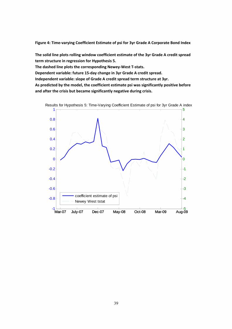
Instead, for each month commencing from March 2007, I run times-series regressions ondaily observations for the next quarter. For each type of regressions specified later, I thenobtain 30 sets of coefficient estimates and Newey-West t-stats. I report these estimatesand t-stats in Table 1-3 to see the time-varying patterns of realized negative basis tradingexcess return’s exposure to systematic risk factors and other factors. I also plot the coeffi-cient estimates for certain factors to highlight the time-varying patterns that are consistentwith the model’s predictions. If basis trading return in excess of funding costs representscompensation from taking systematic risk, then the regression results will have significantcoefficient estimates for systematic risk factors. I run the following two regressions to testthe above Hypothesis 1:

Regression A

RERnbtt,t+k = β0 + β1(LIBOR− FFR)t,t+k + β2FFRt,t+k + β3TEDt,t+k + β4(TED ∗ASW )t,t+k

+β5Basist + εA,t (36)

Regression B


+β5Basist + β6MKTRFt,t+k + β7DEFt,t+k + β8TERMt,t+k + εB,t (37)

Because the funding costs in the calculation of basis trading profits may not be accurateenough, I include 4 terms to control for potential mis-measurement of funding costs in Re-gression A to see if funding costs can explain the realized return of negative basis trading,which is given by the absolute value of RER of negative basis trading. The four controlterms are Libor-FFR, FFR, TED spread and TED*ASW, where FFR is the federal funds

21

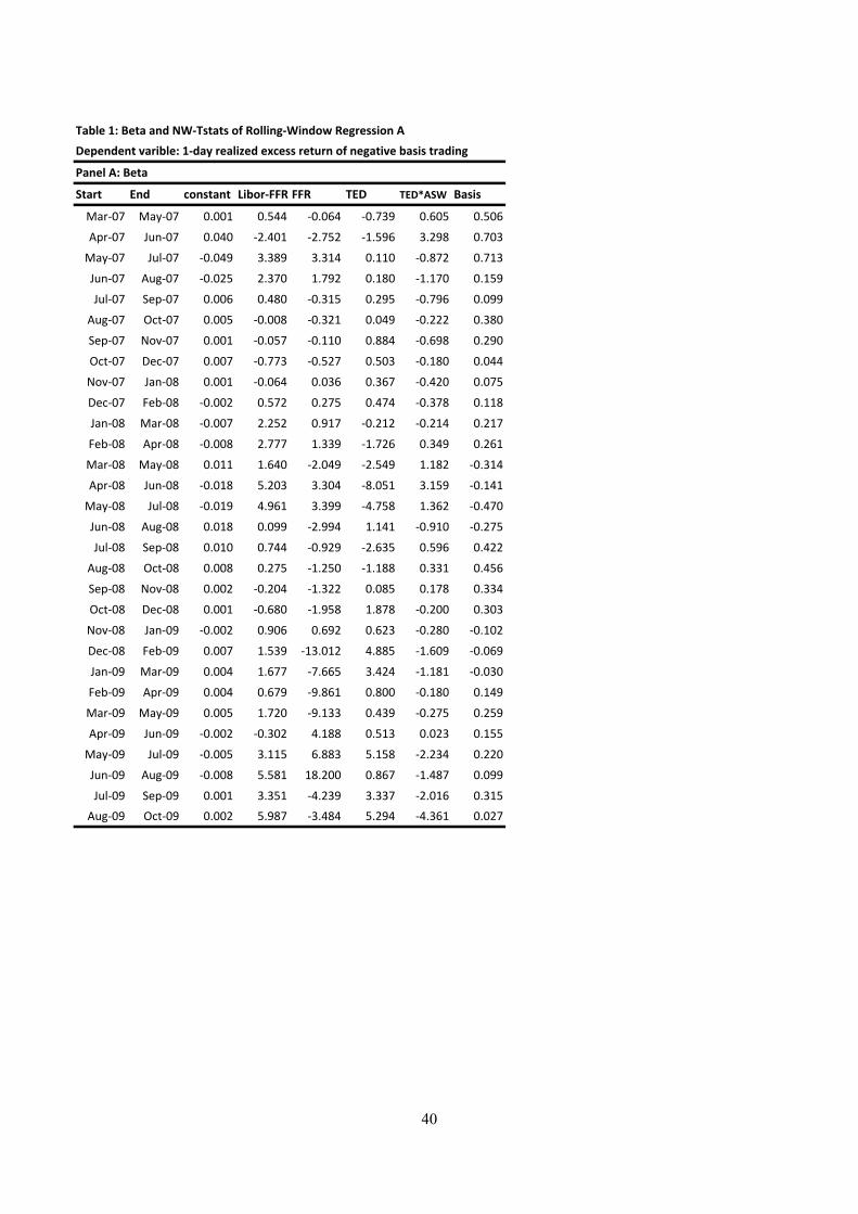
rate. The TED*ASW term accounts for the effect from the mis-measurement of the hair-cut. I also include Basis as an independent variable. Basis is calculated as the average CDSbasis of a number of individual entities. Conventional thinking regards negative basis assignal for profit in doing negative basis trading. But the model doesn’t suggest any relation-ship between the level of basis and basis trading returns. Therefore, I include this variableto test whether there’s any significance relationship. In Regression B, I added three of theFama-French five factors, the MKTRF factor is the excecss return of the market portfolio,the DEF factor is the liquid corporate bond index return minus the T-Note index return ofsimilar maturity9, and the TERM factor is the T-Note return minus the T-Bill return fromKenneth French’s website. I use factor value that are contemporaneous with dependentvariable.

As can be seen from Table 1, funding cost variables are significant during month 13-20,which correspond to the period from Bear Stearn’s crisis to the end of 2008. This suggeststhere may be some mis-measurement in the funding costs when calculating realized returns,but also suggests funding costs have important roles in justifying the return of basis tradingduring the crisis. The Basis factor is not significant for 27 out of 30 rolling windows. Thisis consistent with the model. It highlights the importance of not relying on observed pricediscrepancy when doing risky arbitrage because the signal given by price discrepancy isaffected by the existence of arbitrage cost such as funding costs.

However, funding costs variables along are not good enough to explain the return of negativebasis trading. Regression A has significant intercept estimates in most windows. AddingFama-French factors doesn’t reduce the significance of intercepts by much, but the Fama-French factors are indeed significant and the betas are indeed time-varying as predictedby the model. As shown in Table 2 and Figure 2, beta for DEF factor is significantlynegative for the early periods but not very significant in later periods, while beta for TERMfactor is not very significant for the early periods but is significantly positive in later peri-ods. Kim et.al.(2010) has shown that corporate bond returns during the same period hasnegative exposure to DEF factor and positive exposure to TERM factor. According to themodel, when corporate bond market investors are selling, corporate bond returns are moresensitive to risk factors than CDS, therefore negative basis trading return’s exposures torisk factors should have the same signs as that of the corporate bond return. This point iswell supported by the above findings.

Hypothesis 2: Interaction of funding liquidity and market liquidity predicts abnormalbasis trading return

According to the model, the expected excess profit of basis trading is driven by the in-teraction of funding costs and local investors’ demand. Therefore, I add two other terms toRegression B in order to better explain the abnormal returns of basis trading. The first term

9calculated based on Markit iBoxx 1-10yrs USD Domestic Treasury Index

22

SignedTV is the time t corporate bond market trading volume signed by price changes fromt − 1 to t. This term accounts for the momentum driven by market liquidity. The secondterm is TED spread squared times adjusted trading volume, where the adjusted tradingvolume is calculated as the corporate bond market trading volume minus its -45 days to+45 days median. This adjusted trading volume term is aimed to model the absolute valueof demand shocks in local investors demand, i.e. |zt|. This TED2

t ∗AdjTVt term is impliedby the formula for negative basis trading return in the model.

Regression C


+β5Basist + β6MKTRFt,t+k + β7DEFt,t+k + β8TERMt,t+k

+β9SignedTVt + β10TED2t ∗AdjTVt + εB,t (38)

As shown in Table 3, the SignedTV term is significantly positive for most windows. Thisis not surprising as negative basis trading consists of buying corporate bond, which ispositively affected by the momentum in corporate bond returns. The TED2

t ∗AdjTVt termis significantly negative during the latter half of 2008. This is highly consistent with themodel’s prediction. Proposition 3 suggests that negative basis trading return is increasingin α and −zt, which during the later half of 2008 are well proxied by TED spread andadjusted corporate bond trading volume respectively. More importantly, Regression Cresults in insignificant intercepts for most windows, and the Basis factor is not significantfor almost all windows.

4.3 Term Structure of Basis Trading Profit

Proposition 5 predicts that absolute value of basis trading return, which is also the profitof basis trading, is increasing in the time to maturity of the underlying bond. I comparedthe profits of basis trading on underlyings with 2 years, 5 years and 9 years time to maturity.I list the average 1-day, 1-week and 1-month holding period profits for these maturities inTable 4, which clearly shows that basis trading on longer maturities earn higher profits.

This result is also shown by the plot of cumulative 1-week profits of basis trading on thesematurities in Figure 3. Basis trading on longer maturities have higher cumulative profits,and the gaps between the lines are also increasing over time, which is consistent with theprediction that basis trading profit is increasing in the time to maturity of the underlyingbond.

4.4 Comparative Statics on Basis Trading and the CDS Basis

The model yields several testable comparative statics results. The purpose here is to showthat more severe market frictions make basis trading more risky, hence earning higher ex-pected return. To be specific, I tested the following predictions:

23

Hypothesis 3:

• The size of basis trading return is increasing in αc and σλ.

• Basis trading is risky, the size of basis trading return is increasing in the volatility ofbasis trading return.

• The volatility of basis trading return is increasing in αc, which is proxied by TEDspread.

The volatility of basis trading return is the next 90-day volatility of the negative basistrading RER. To test the comparative statics results, I sort the time-series of the absolutevalue and volatility of basis trading returns of different holding periods based on their cor-responding TED and default intensity volatility values. For instance, I assign each date inthe sample period into 5 groups according to the TED spread value at each date, the firstgroup contains dates with the lowest TED spread values, the 5th group contains dates withthe highest TED spread values. Then I calculate the median value of the absolute valueof negative basis trading return for each group, and report in a table to see if the groupwith higher TED spread also has larger basis trading return size. I also sort the sizes ofbasis trading return into negative basis trading volatility groups. Results are summarizedin Table 5, in which each panel provides result of each comparative statics. In general, theresults support Hypothesis 3 very well.

Using the similar approach, I test the prediction from Proposition 4 that CDS basisis increasing in the demand shock on corporate bond market. The results in Proposition4 are given conditional on the sign of local investors’ demand on cash market. Togetherwith the result on the sign of basis trading returns and the assumption that basis is morelikely to be negative when negative basis trading is profitable and vice versa, I conjecturethat the absolute value of CDS basis is increasing in the absolute value of local investors’demand on corporate bond market, which is proxied by the corporate bond market tradingvolume. Table 6 shows that those dates with larger corporate bond market trading volumehas larger absolute basis. Therefore, the following hypothesis is also supported by the data.

Hypothesis 4: The absolute value of CDS basis is increasing in corporate bond markettrading volume.

4.5 The Predictability of Credit Spread Term Structure Slope on FutureCredit Spread Changes

Hypothesis 5:

• Credit spread term structure slope positively predicts future credit spread changes whenfrictions are small.

24

• Credit spread term structure slope does not positively predict future credit spreadchanges when investors are selling corporate bonds and funding cost has high sensitiv-ity to default intensity. This poor predictability is more likely for shorter maturities.

I carry out the following regressions to test this hypothesis:

CSt+k − CSt = ψ0 + ψSlopet + εt (39)

I used 4 sets of dependent variables and independent variables. For instance, for Set 1,I use the 1-5 years grade A corporate bond index asset swap spread as the CS variable.For this dependent variable, I use the 3-5 years grade A corporate bond index asset swapspread minus the 1-3 years grade A corporate bond index asset swap spread as the Slopevariable. For this set, the dependent variable proxies the future change in credit spreadof a 3-year corporate bond, while the independent variable proxies the difference in creditspreads of a 4 year corporate bond and a 2 year corporate bond issued by the same entity asthe 3-year bond. The independent variable thus proxies the term structure of credit spreadat 3 year. A full list of variables for other sets are listed in Table 7, which also reportsregression results. I test for k =5 days and 15 days respectively and run the regressionson three sub-periods: sub-periods 1 (07/2007 to 02/2008), sub-period 2 (03/2008-03/2009)and sub-periods 3 (04/2009-09/2009) to characterize different levels of market frictions.

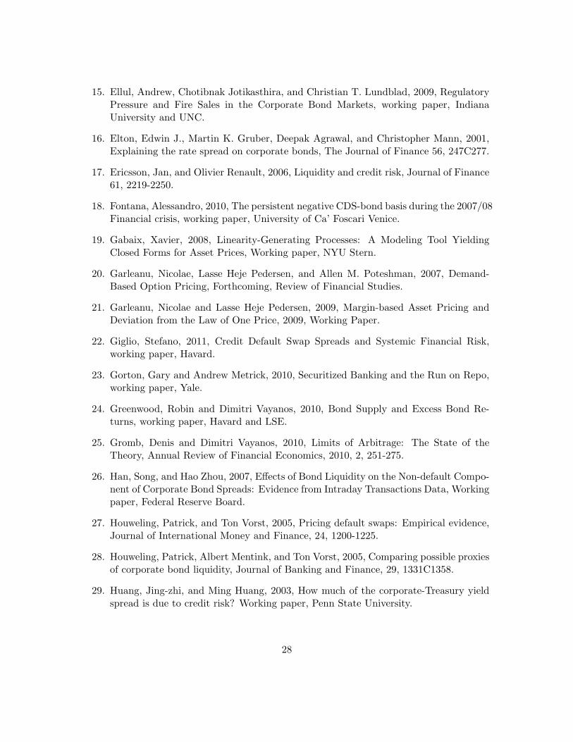
The results are in favor of Hypothesis 5. For sub-periods 1 (07/2007 to 02/2008) andsub-periods 3 (04/2009-09/2009) which corresponds to periods with less market frictions,the positive predictability of the independent variable on dependent variable is found inmost cases. These results are consistent with Bedendo et.al.(2007). But in sub-period 2(03/2008-03/2009) when market frictions are high after the Bear Stern and Lehman Col-lapse, the predictability is lost for Set 1 and Set 3, which correspond to credit spread termstructure at approximately 3 year, while the predictability is still significant for Set 2 andSet 4, which correspond to longer time to maturity at approximately 7.5 year. Such find-ings support the predictions from Proposition 2, which states the regression coefficient ψ ispositive when friction is low but can take negative values when friction is high. Therefore,it’s not surprising to find that the predictability is lost during sub-period 2, in which severefrictions can drive the coefficient negative at times. Using shorter sub-period windows, Ieven find negative coefficient ψ for the 3 year term structure as shown in Figure 4.

4.6 Robustness Checks

The main results are not affected when using alternative funding cost proxies. To test if theresults are sensitive to the construction of the Markit indices, I also construct alternativenegative basis trading returns using individual CDS and corporate bond data. Regressionresults using these returns as dependent variables are consistent with results in the previoussection. But individual CDS and corporate bond data are less reliable than the Markitindices, so I still report results using the Markit indices as the main results.

25

5 Conclusion

The theoretical part of this paper proposes a continuous-time limited arbitarge model toshow how time-varying funding costs and demand pressure jointly create risky arbitrageopportunities on markets with identical assets. The interaction of funding illiquidity andmarket illiquidity results in one assets being more sensitive to risk factors that have non-zero market prices of risk than another asset with identical cash-flow does. Taking oppositepositions on the two markets therefore has non-zero risk exposure and hence non-zero ex-pected excess return. The model is applied to analyze CDS basis trading in closed-form andgenerate a number of testable predictions. Empirically, I find evidence for the time-varyingexposure of basis trading to systematic risks as the Fama-French MKT, DEF and TERMfactors are significant in explaining realized basis trading returns. Factors in the form ofTED spread squared times adjusted corporate bond market trading volume has short-termpredictive power on abnormal basis trading returns. The size and volatility of realized basistrading return is increasing in the severity of market frictions, while basis trading profits areincreasing in the time to maturity of the underlying bond. As predicted by the model, underhigh levels of market frictions, the positive predictability of credit spread term structureslope on future changes in credit spread no longer exists.

26

References

1. Bai, Jennie, and Pierre Collin-Dufresne, The Determinants of the CDS-Bond BasisDuring the Financial Crisis of 2007-2009, 2010, Working Paper, Federal Reserve Bankof New York and Columbia.

2. Bedendo, Mascia, Lara Cathcart, and Lina El-Jahel, 2007, The Shape of the TermStructure of Credit Spreads: An Empirical Investigation, Journal of Financial Re-search, Vol. 30, No. 2.

3. Berndt, Antje, Rohan Douglas, Darrell Duffie, Mark Ferguson, and David Schranz,2009, Measuring default risk premia from default swap rates and EDFs, Workingpaper.

4. Bongaerts, Dion, Frank De Jong, and Joost Driessen, 2008, Liquidity and liquidityrisk premia in the CDS market, Working Paper, University of Amsterdam.

5. Blanco, Roberto, Simon Brennan, and Ian W. Marsh, 2005, An empirical analysis ofthe dynamic relationship between investment grade bonds and credit default swaps,Journal of Finance 60, 2255-2281.

6. Buhler, Wolfgang and Monika Trapp, 2009, Time-Varying Credit Risk and LiquidityPremia in Bond and CDS Markets, Working Paper.

7. Chen, Long, David A. Lesmond, and Jason Wei, 2007, Corporate yield spreads andbond liquidity, Journal of Finance 62, 119-149.

8. Choudhry, Moorad, 2006, Revisiting the Credit Default Swap Basis: Further Analysisof the Cash and Synthetic Credit Market Differential, Journal of Structured Finance,Winter 2006, 21-32.

9. Collin-Dufresne, Pierre, Robert S. Goldstein, and J. Spencer Martin, 2001, The de-terminants of credit spread changes, Journal of Finance 56, 2177C2207.

10. Das Sanjiv R. and Paul Hanouna, 2009, Hedging credit: Equity liquidity matters, J.Finan. Intermediation 18, 112C123.

11. Driessen, J. 2005, Is Default Event Risk Priced in Corporate Bonds? Review ofFinancial Studies 18, 165C195.

12. Duffie, Darrell, 1999, Credit swap valuation, Financial Analysts Journal, January/February,73-87.

13. Duffie, Darrell, 2004, Credit Risk Modeling with Affine Processes, Cattedra GalileanaLectures.

14. Duffie, Darrell, and Kenneth J. Singleton, 1999, Modeling term structures of default-able bonds, Review of Financial Studies 12, 687C720.

27

15. Ellul, Andrew, Chotibnak Jotikasthira, and Christian T. Lundblad, 2009, RegulatoryPressure and Fire Sales in the Corporate Bond Markets, working paper, IndianaUniversity and UNC.

16. Elton, Edwin J., Martin K. Gruber, Deepak Agrawal, and Christopher Mann, 2001,Explaining the rate spread on corporate bonds, The Journal of Finance 56, 247C277.

17. Ericsson, Jan, and Olivier Renault, 2006, Liquidity and credit risk, Journal of Finance61, 2219-2250.

18. Fontana, Alessandro, 2010, The persistent negative CDS-bond basis during the 2007/08Financial crisis, working paper, University of Ca’ Foscari Venice.

19. Gabaix, Xavier, 2008, Linearity-Generating Processes: A Modeling Tool YieldingClosed Forms for Asset Prices, Working paper, NYU Stern.

20. Garleanu, Nicolae, Lasse Heje Pedersen, and Allen M. Poteshman, 2007, Demand-Based Option Pricing, Forthcoming, Review of Financial Studies.

21. Garleanu, Nicolae and Lasse Heje Pedersen, 2009, Margin-based Asset Pricing andDeviation from the Law of One Price, 2009, Working Paper.

22. Giglio, Stefano, 2011, Credit Default Swap Spreads and Systemic Financial Risk,working paper, Havard.

23. Gorton, Gary and Andrew Metrick, 2010, Securitized Banking and the Run on Repo,working paper, Yale.

24. Greenwood, Robin and Dimitri Vayanos, 2010, Bond Supply and Excess Bond Re-turns, working paper, Havard and LSE.

25. Gromb, Denis and Dimitri Vayanos, 2010, Limits of Arbitrage: The State of theTheory, Annual Review of Financial Economics, 2010, 2, 251-275.

26. Han, Song, and Hao Zhou, 2007, Effects of Bond Liquidity on the Non-default Compo-nent of Corporate Bond Spreads: Evidence from Intraday Transactions Data, Workingpaper, Federal Reserve Board.

27. Houweling, Patrick, and Ton Vorst, 2005, Pricing default swaps: Empirical evidence,Journal of International Money and Finance, 24, 1200-1225.

28. Houweling, Patrick, Albert Mentink, and Ton Vorst, 2005, Comparing possible proxiesof corporate bond liquidity, Journal of Banking and Finance, 29, 1331C1358.

29. Huang, Jing-zhi, and Ming Huang, 2003, How much of the corporate-Treasury yieldspread is due to credit risk? Working paper, Penn State University.

28

30. Hull, John, Mirela Predescu, and Alan White, 2004, The relationship between creditdefault swap spreads, bond yields, and credit rating announcements, Journal of Bank-ing and Finance 28, 2789-2811.

31. Jarrow, Robert, 2004, Risky Coupon Bonds as a Portfolio of Zero-Coupon Bonds,Finance Research Letters 1 (2004) 100C105.

32. Jarrow, Robert, David Lando, and Fan YU, 2005, Default Risk and Diversification:Theory and Empirical Implications, Mathematical Finance 15(1), 1-26.

33. Jeanblanc, Monique, and Stoyan Valchev, 2007, Default-risky bond prices with jumps,liquidity risk and incomplete information. Decisions Econ Finan (2007) 30:109C136.

34. Jurek, Jakub W. and Erik Stafford, 2011, Crashes and Collateralized Lending, workingpaper, Princeton and Harvard.

35. Kim, Gi Hyun, Haitao Li, and Weina Zhang, 2010, The CDS/Bond Basis and theCross Section of Corporate Bond Returns, working paper, University of Michigan andNUS.

36. Longstaff, Francis A., Sanjay Mithal, and Eric Neis, 2005, Corporate yield spreads:Default risk or liquidity? New evidence from credit-default swap market, Journal ofFinance 60, 2213-2253.

37. Mitchell, Mark, and Todd Pulvino, 2011, Arbitrage Crashes and the Speed of Capital,Journal of Financial Economics, Forthcoming.

38. Naranjo, Lorenzo, 2008, Implied Interest Rates in a Market with Frictions, WorkingPaper. NYU Stern.

39. Nashikkar, Amrut, and Marti Subrahmanyam, 2006, Latent liquidity and corporatebond yield spreads, Working paper, NYU Stern.

40. Pan, Jun, and Kenneth J. Singleton, 2005, Default and recovery implicit in the termstructure of sovereign CDS spreads, Working paper, MIT and Stanford.

41. Tang, Dragon-Yongjun. and Hong Yan, 2007, Liquidity and Credit Default SwapSpreads. Working Paper. University of South Carolina and Kennesaw State Univer-sity.

42. Tuckman Bruce and Jean-Luc Vila, 1992, Arbitrage with funding costs: a utility-basedapproach. Journal of Finance 47:1283-1302.

43. Vayanos, Dimitri and Jean-Luc Vila, 2009, A Preferred-Habitat Model of the TermStructure of Interest Rates. Working Paper, London School of Economics and MerrillLynch.

29

44. Vayanos, Dimitri and Jiang Wang, 2009, Liquidity and Asset Prices: A Unified Frame-work, working paper, LSE and MIT.

45. Yu, Fan, 2003, Dependent Default in Intensity-Based Models, Working Paper, Clare-mont Mckenna College.

46. Zhu, Haibin, 2006, An Empirical Comparison of Credit Spreads between the BondMarket and the Credit Default Swap Market, Journal of Financial Services Research29, 211-235.

30

6 Appendix A: Motivation for the Funding Costs Function

6.1 Borrowing Costs

Assume there’s a continuum of competitive cash lenders lends yt cash for 1-dollar worth ofbond.

maxyt

[Et(dwt)−γ

2V art(dwt)] (40)

dwt = (wt − yt)rtdt+ yt(rt + s)dt+ [(1− L)− yt]dNt (41)

where Nt is counting process for the borrower’s default, the intensity of Nt is f(λt) whichis increasing in λt. s > 0 is the exogenous rate above short-rate asked by the lender forlending using the risky bond as collateral.

y∗t = s/[γf(λt)]− 1/γ + (1− L) (42)

Therefore y∗t is decreasing in f(λt), thus decreasing in λt. The borrower borrows y∗t fractionof her bond purchase at rt+s and 1−y∗t fraction at rt+u, where u > 0 reflects the differencebetween un-collateralized rate and risk-free short rate. So the borrow cost in excess of rt is:

ht = y∗t (rt + s) + (1− y∗t )(rt + u)− rt = u− (u− s)y∗t (43)

which is a decreasing function of y∗t . Since y∗t is decreasing in λt, the borrow cost ht isincreasing in λt. With careful choice of the exogenous f(λt), the borrow cost has the linearfunctional form of αλt + δ as in the model.

6.2 Short-selling Costs

Assume there’s a continuum of competitive bond lenders requires yt cash for 1-dollar worthof bond.

maxyt

[Et(dwt)−γ

2V art(dwt)] (44)

dwt = (wt + yt)rtdt+ yt(rt − s)dt+ (yt − 1)dNt (45)

where Nt is counting process for the short-seller’s default, the intensity of Nt is g(λt) whichis decreasing in λt. s > 0 is the exogenous special repo rate offered by the bond lender onthe cash collateral.

y∗t = s/[γg(λt)] + 1/γ + 1 (46)

Therefore y∗t is decreasing in g(λt), thus increasing in λt. The short-seller lends y∗t fractionof her bond sales at rt − s and 1− y∗t fraction at rt. So her short selling cost is:

ht = rt − [y∗t (rt − s) + (1− y∗t )rt] = sy∗t (47)

which is a increasing function of y∗t . Since y∗t is also increasing in λt, the short-selling costht is increasing in λt. With careful choice of the exogenous g(λt), the short-selling cost hasthe linear functional form of αλt + δ as in the model.

31

7 Appendix B: Proofs of Lemma and Proposition

7.1 Proof of Lemma 1

In the most general set-up, there’re 4 sources of uncertainties, one is the jump at default,characterized by Nt, and three others as the Brownian Motions in the default intensity λt,short rate rt and local investors’ demand shock zt, i.e. Bλ,t, Br,t and Bz,t. The dynamicof Nt only enters into play through λt, so I can rewrite P d

t (τ) as P dt (τ, λ, r, z) and P c

t (τ) asP c

t (τ, λ, r, z). Assuming all three Brownian Motions Bλ,t, Br,t and Bz,t are independent, Iapply Ito’s lemma to write dP c

t (τ, λ, z) and dP dt (τ, λ, z) as:

dP ct (τ, λ, r, z) = µc

t(τ)Pct dt+ σλ

∂P

∂λdBλ,t + σr

∂P

∂rdBr,t + σz

∂P

∂zdBz,t (48)

dP dt (τ, λ, r, z) = µd

t (τ)Pdt dt+ σλ

∂V

∂λdBλ,t + σr

∂V

∂rdBr,t + σz

∂V

∂zdBz,t (49)

where µct and µd

t are the expected returns of the bond C and bond D, conditional onno default. Entering the above dynamic into the arbitrageur’s optimization problem anddropping τ , I derive the F.O.C. as in Lemma 1.


Applying Ito’s lemma, the dP dt /P

dt and dP c

t /Pct terms can be re-written as:

dP ct (τ)

P ct (τ)

= µct(τ)dt−Ac

λσλdBλ,t −AcrσrdBr,t (50)

dP dt (τ)

P dt (τ)

= µdt (τ)dt−Ad

λσλdBλ,t −AdrσrdBr,t (51)

where, omitting τ , the instantaneous expected returns conditional on no default are:

µct = −Ac

λκλ(λ− λt)−Aczκr(r − rt) +Ac

λ′λt +Ac

r′rt + Cc′ +

12Ac

λ2σ2

λ +12Ac

r2σ2

r (52)

µdt = −Ad

λκλ(λ− λt)−Adrκr(r − rt) +Ad

λ′λt +Ad

r′rt + Cd′ +

12Ad

λ2σ2

λ +12Ad

r2σ2

r (53)

Substitute the above into the dynamic budget constraint, the arbitrageur’s F.O.C.s are:

µct(τ)− rt − hc

t(τ)|xc

t(τ)|xc

t(τ)− Lλt = LΦJ,t − σλA

cλ(τ)Φλ,t − σrA

cr(τ)Φr,t (54)

µdt (τ)− rt − hd

t (τ)|xd

t (τ)|xd

t (τ)− Lλt = LΦJ,t − σλA

dλ(τ)Φλ,t − σrA

dr(τ)Φr,t (55)

where

ΦJ,t = γL

∫ T

0[xd

t (τ) + xct(τ)]dτλt (56)

32

Φλ,t = γσλ

∫ T

0[−xd

t (τ)Adλ(τ)− xc

t(τ)Acλ(τ)]dτ (57)

Φr,t = γσr

∫ T

0[−xd

t (τ)Adr(τ)− xc

t(τ)Acr(τ)]dτ (58)

are the market prices of risks to the default jump, default intensity and short rate factors.

In equilibrium, markets clear. So xit + zi = 0, i = c, d. Replace xi

t(τ) by −zi(τ), andreplace hi

t by the functions defined in previous sections, then the F.O.C.s are affine equa-tions in the risk factors λt and rt. Setting the linear terms in λt and rt to zero implies thatAi

j(τ) are the solutions to the a system of ODEs with initial conditions Aij(0) = 0, i = v, p

and j = λ, r:

Acλ′(τ) + κλA

cλ(τ)− [−αc(τ)

|zc(τ)|zc(τ)

+ L] = −γL2∫ T

0[zd(τ) + zc(τ)]dτ (59)

Adλ′(τ) + κλA

dλ(τ)− [−αd(τ)

|zd(τ)|zd(τ)

+ L] = −γL2∫ T

0[zd(τ) + zc(τ)]dτ (60)

Acr′(τ) + κrA

cr(τ)− 1 = 0 (61)

Adr′(τ) + κrA

dr(τ)− 1 = 0 (62)

7.3 Proof of Proposition 1

Replace ∂P ct

∂λ /Pct with −Ac

λ(τ) and replace ∂P dt

∂λ /Pdt with −Ad

λ(τ) in Definition 1, ∂P ct

∂r /Pct

and ∂P ct

∂r /Pct are the same.


The time-varying component in the dependent variable is: Acλ(τ−∆τ)

τ−∆τ λt+∆τ −Ac

λ(τ)

τ λt, the

time-varying componet in the independent variable is: Acλ(τ)

τ λt−Ac

λ(τ−∆τ)

τ−∆τ λt. So the regres-sion coefficient is:

ψ =cov[Ac

λ(τ−∆τ)

τ−∆τ λt+∆τ −Ac

λ(τ)

τ λt,Ac

λ(τ)

τ λt −Ac

λ(τ−∆τ)

τ−∆τ λt]

var[Acλ(τ)

τ λt −Ac

λ(τ−∆τ)

τ−∆τ λt](63)

=τAc

λ(τ −∆τ)e−κλ∆τ − (τ −∆τ)Acλ(τ)

(τ −∆τ)Acλ(τ)− τAc

λ(τ −∆τ)(64)

when ∆τ → 0,

ψ = −τ [Acλ(τ)′ + κλA

cλ(τ)]

τ [Acλ(τ)′ − 1]

(65)

=F (τ)

1− F (τ)e−κλτ(66)

33

where F (τ) = −αc(τ) |zc(τ)|

zc(τ) + L− γL2∫ T0 [zc(τ) + zd(τ)]dτ .

ψ > 0 if F (τ) < eκλτ , and ψ < 0 if F (τ) > eκλτ .


Lemma 3a: For very negative θ(τ) and negative θ(τ), the Arbitrageur’s F.O.C.s are:

µct(τ)− rt − hc

t(τ)− Lλt = LΦJ,t − σλAcλ(τ)Φλ,t − σrA

cr(τ)Φr,t − σzA

cz(τ)Φz,t (67)

µdt (τ)− rt + hd

t (τ)− Lλt = LΦJ,t − σλAdλ(τ)Φλ,t − σrA

dr(τ)Φr,t − σzA

dz(τ)Φz,t (68)

where

ΦJ,t = γL

∫ T

0[xd

t (τ) + xct(τ)]dτλt (69)

Φλ,t = γσλ

∫ T

0[−xd

t (τ)Adλ(τ)− xc

t(τ)Acλ(τ)]dτ (70)

Φr,t = γσr

∫ T

0[−xd

t (τ)Adr(τ)− xc

t(τ)Acr(τ)]dτ (71)

Φz,t = γσz

∫ T

0[−xd

t (τ)Adz(τ)− xc

t(τ)Acz(τ)]dτ (72)

are the market prices of risks to the default jump, default intensity, short rate and demandshock factors.

In equilibrium, markets clear. So xit + zi

t = 0. Then the F.O.C.s are affine equationsin the risk factors λt, rt and zt.10 Setting the linear terms in λt, rt and zt to zero impliesthat Ai

j(τ) are the solutions to the a system of ODEs with initial conditions Aij(0) = 0,

i = v, p and j = λ, r, z:

Acλ′(τ) + κλA

cλ(τ)− [αc(τ) + L] = 0 (73)

Adλ′(τ) + κλA

dλ(τ)− [−αd(τ) + L] = 0 (74)

Acr′(τ) + κrA

cr(τ)− 1 = 0 (75)

Adr′(τ) + κrA

dr(τ)− 1 = 0 (76)

Acz′(τ) + κzA

cz(τ) = −γσ2

λAcλ(τ)

∫ T

0θ(τ)[Ac

λ(τ)−Adλ(τ)]dτ − γσ2

zAcz(τ)

∫ T

0θ(τ)[Ac

z(τ)−Adz(τ)]dτ

(77)

Adz′(τ) + κzA

dz(τ) = −γσ2

λAdλ(τ)

∫ T

0θ(τ)[Ac

λ(τ)−Adλ(τ)]dτ − γσ2

zAdz(τ)

∫ T

0θ(τ)[Ac

z(τ)−Adz(τ)]dτ

(78)

Lemma 3b: similar to Lemma 3a, but the unique positive solution of κ∗z is guaranteed onlywhen κz is large enough.

10By assuming that the two markets have exact opposite demand pressure, the market price of risk forthe default jump factor becomes zero as the arbitrageur’s aggregate positions are free of default jump risk.

34


Replace ∂P ct

∂λ /Pct with −Ac

λ(τ), replace ∂P dt

∂λ /Pdt with −Ad

λ(τ), replace ∂P ct

∂z /Pct with −Ac

z(τ),

replace ∂P dt

∂z /Pdt with −Ad

z(τ) in Definition 1, ∂P ct

∂r /Pct and ∂P c

t∂r /P

ct are the same.


∂Basis

∂λt=

Adλ(τ)τ

− Acλ(τ)τ

(79)

∂Basis

∂zt=

Adz(τ)τ

− Acz(τ)τ

(80)

so sign(∂Basis∂λt

) = sign(Adλ −Ac

λ) and sign(∂Basis∂zt

) = sign(Adz −Ac

z).


Easily proved by taking the derivatives of Gλ(τ) and Gz(τ) on τ , then summarize resultsfor different signs of zc

t (τ).


∂2Yt(τ)/∂τ = [Acλ(τ)

τ ]′λt + constants, where Acλ(τ)

τ = [αc + L]1−e−κλτ

κλτ when zct < 0 and

Acλ(τ)

τ = [−αc + L]1−e−κλτ

κλτ when zct > 0. 1−e−κλτ

κλτ is a decreasing function of τ , therefore

∂2Yt(τ)/(∂τ∂λt) = [Acλ(τ)

τ ]′ < 0. When zct < 0, [Ac

λ(τ)

τ ]′ = [αc+L](1−e−κλτ

κλτ )′ is more negative

than [Acλ(τ)

τ ]′ = [−αc + L](1−e−κλτ

κλτ )′ when zct > 0.

35

Appendix C: Figures and Tables

Figure 1: CDS Basis and 1‐week Negative Basis Trading Returns

Dashed line plots CDS basis from April 2007 to December 2009.

Values in the left vertical axis are in basis points.

Solid line plots 1‐week realized excess return of negative basis trading.

04/07 08/07 03/08 10/08 12/08 04/09 12/09-500

0

500Basis vs Negative Basis Trading Return (1-week holding period)

04/07 08/07 03/08 10/08 12/08 04/09 12/09-5%

0%

5%

Basis (cds price - credit spread)

Negative Basis Trading Return

36

Figure 2: Negative Basis Trading Return’s Time‐varying Exposure to Systematic Factors

The solid line plots rolling window beta of the DEF factor in Regression B.

The dashed line plots rolling window beta of the TERM factor in Regression B.

Dependent variable: 1‐day realized excess return of negative basis trading.

As predicted by the model, betas are highly time‐varying.

Mar-07 July-07 Dec-07 May-08 Oct-08 Mar-09 Aug-09-1.5

-1

-0.5

0

0.5

1

1.5 Basis Trading Return's Time-varying Beta on Systematic Factors

beta of DEF in regression B

beta of TERM in regression B

37

Figure 3: Cumulative Profit of Basis Trading on Underlying of Different Maturities

The three lines plot the cumulative sum of the absolute value of negative CDS basis trading

returns on underlying bonds of three different maturities.

Size of basis trading return is larger for underlying bond with longer time to maturity.

01/01/2007 01/01/2008 01/01/2009 01/01/20100

0.5

1

1.5

2

2.5

3

3.5

4Cumulative Profit of Basis Trading on Underlyings of Different Maturities

cumulative basis trading profit on 2yr underlying

cumulative basis trading profit on 5yr underlyingcumulative basis trading profit on 10yr underlying

38

Figure 4: Time‐varying Coefficient Estimate of psi for 3yr Grade A Corporate Bond Index

The solid line plots rolling window coefficient estimate of the 3yr Grade A credit spread

term structure in regression for Hypothesis 5.

The dashed line plots the corresponding Newey‐West T‐stats.

Dependent variable: future 15‐day change in 3yr Grade A credit spread.

Independent variable: slope of Grade A credit spread term structure at 3yr.

As predicted by the model, the coefficient estimate psi was significantly positive before

and after the crisis but became significantly negative during crisis.

Mar-07 July-07 Dec-07 May-08 Oct-08 Mar-09 Aug-09-1

-0.8

-0.6

-0.4

-0.2

0

0.2

0.4

0.6

0.8

1Results for Hypothesis 5: Time-Varying Coefficient Estimate of psi for 3yr Grade A index

Mar-07 July-07 Dec-07 May-08 Oct-08 Mar-09 Aug-09-5

-4

-3

-2

-1

0

1

2

3

4

5

coefficient estimate of psi

Newey West tstat

39

Table 1: Beta and NW‐Tstats of Rolling‐Window Regression A

Dependent varible: 1‐day realized excess return of negative basis trading

Panel A: Beta

Start End constant Libor‐FFR FFR TED TED*ASW Basis

Mar‐07 May‐07 0.001 0.544 ‐0.064 ‐0.739 0.605 0.506

Apr‐07 Jun‐07 0.040 ‐2.401 ‐2.752 ‐1.596 3.298 0.703

May‐07 Jul‐07 ‐0.049 3.389 3.314 0.110 ‐0.872 0.713

Jun‐07 Aug‐07 ‐0.025 2.370 1.792 0.180 ‐1.170 0.159

Jul‐07 Sep‐07 0.006 0.480 ‐0.315 0.295 ‐0.796 0.099

Aug‐07 Oct‐07 0.005 ‐0.008 ‐0.321 0.049 ‐0.222 0.380

Sep‐07 Nov‐07 0.001 ‐0.057 ‐0.110 0.884 ‐0.698 0.290

Oct‐07 Dec‐07 0.007 ‐0.773 ‐0.527 0.503 ‐0.180 0.044

Nov‐07 Jan‐08 0.001 ‐0.064 0.036 0.367 ‐0.420 0.075

Dec‐07 Feb‐08 ‐0.002 0.572 0.275 0.474 ‐0.378 0.118

Jan‐08 Mar‐08 ‐0.007 2.252 0.917 ‐0.212 ‐0.214 0.217

Feb‐08 Apr‐08 ‐0.008 2.777 1.339 ‐1.726 0.349 0.261

Mar‐08 May‐08 0.011 1.640 ‐2.049 ‐2.549 1.182 ‐0.314

Apr‐08 Jun‐08 ‐0.018 5.203 3.304 ‐8.051 3.159 ‐0.141

May‐08 Jul‐08 ‐0.019 4.961 3.399 ‐4.758 1.362 ‐0.470

Jun‐08 Aug‐08 0.018 0.099 ‐2.994 1.141 ‐0.910 ‐0.275

Jul‐08 Sep‐08 0.010 0.744 ‐0.929 ‐2.635 0.596 0.422

Aug‐08 Oct‐08 0.008 0.275 ‐1.250 ‐1.188 0.331 0.456

Sep‐08 Nov‐08 0.002 ‐0.204 ‐1.322 0.085 0.178 0.334

Oct‐08 Dec‐08 0.001 ‐0.680 ‐1.958 1.878 ‐0.200 0.303

Nov‐08 Jan‐09 ‐0.002 0.906 0.692 0.623 ‐0.280 ‐0.102

Dec‐08 Feb‐09 0.007 1.539 ‐13.012 4.885 ‐1.609 ‐0.069

Jan‐09 Mar‐09 0.004 1.677 ‐7.665 3.424 ‐1.181 ‐0.030

Feb‐09 Apr‐09 0.004 0.679 ‐9.861 0.800 ‐0.180 0.149

Mar‐09 May‐09 0.005 1.720 ‐9.133 0.439 ‐0.275 0.259

Apr‐09 Jun‐09 ‐0.002 ‐0.302 4.188 0.513 0.023 0.155

May‐09 Jul‐09 ‐0.005 3.115 6.883 5.158 ‐2.234 0.220

Jun‐09 Aug‐09 ‐0.008 5.581 18.200 0.867 ‐1.487 0.099

Jul‐09 Sep‐09 0.001 3.351 ‐4.239 3.337 ‐2.016 0.315

Aug‐09 Oct‐09 0.002 5.987 ‐3.484 5.294 ‐4.361 0.027

40

Table 1 Continued: Beta and NW‐Tstats of Rolling‐Window Regression A


Panel B: Newey West Tstat

Start End constant Libor‐FFR FFR TED TED*ASW Basis

Mar‐07 May‐07 0.022 0.153 ‐0.018 ‐1.338 1.210 1.503

Apr‐07 Jun‐07 0.504 ‐0.501 ‐0.505 ‐1.581 1.750 1.965

May‐07 Jul‐07 ‐1.755 2.169 1.765 0.111 ‐0.684 1.224

Jun‐07 Aug‐07 ‐2.641 3.988 2.655 0.192 ‐1.332 0.385

Jul‐07 Sep‐07 0.550 0.779 ‐0.429 0.302 ‐0.773 0.248

Aug‐07 Oct‐07 0.879 ‐0.012 ‐0.650 0.050 ‐0.247 1.647

Sep‐07 Nov‐07 0.126 ‐0.084 ‐0.132 1.846 ‐1.640 1.367

Oct‐07 Dec‐07 1.616 ‐1.891 ‐1.407 0.985 ‐0.561 0.251

Nov‐07 Jan‐08 0.334 ‐0.127 0.128 0.308 ‐0.501 0.274

Dec‐07 Feb‐08 ‐0.590 0.941 0.763 0.398 ‐0.612 0.392

Jan‐08 Mar‐08 ‐0.993 1.849 0.974 ‐0.082 ‐0.167 0.698

Feb‐08 Apr‐08 ‐0.838 1.833 0.799 ‐0.715 0.359 0.597

Mar‐08 May‐08 0.373 0.454 ‐0.388 ‐0.878 1.870 ‐1.066

Apr‐08 Jun‐08 ‐1.985 3.651 2.078 ‐2.765 2.139 ‐0.515

May‐08 Jul‐08 ‐2.055 3.395 1.991 ‐2.464 1.538 ‐2.239

Jun‐08 Aug‐08 1.370 0.089 ‐1.186 0.758 ‐1.798 ‐1.524

Jul‐08 Sep‐08 2.900 1.581 ‐1.585 ‐2.629 2.225 1.802

Aug‐08 Oct‐08 2.884 0.430 ‐2.405 ‐0.868 1.004 2.506

Sep‐08 Nov‐08 1.298 ‐0.254 ‐2.975 0.059 0.590 1.835

Oct‐08 Dec‐08 0.845 ‐0.671 ‐1.512 1.021 ‐0.507 1.704

Nov‐08 Jan‐09 ‐1.115 0.883 0.337 0.297 ‐0.514 ‐0.575

Dec‐08 Feb‐09 3.081 1.067 ‐3.909 2.042 ‐2.520 ‐0.456

Jan‐09 Mar‐09 1.153 1.635 ‐1.315 1.345 ‐1.682 ‐0.218

Feb‐09 Apr‐09 1.258 0.519 ‐1.319 0.855 ‐1.218 0.892

Mar‐09 May‐09 2.264 1.288 ‐1.807 0.462 ‐1.004 1.675

Apr‐09 Jun‐09 ‐0.695 ‐0.084 0.620 0.232 0.085 0.763

May‐09 Jul‐09 ‐1.641 1.009 0.914 1.370 ‐1.897 0.725

Jun‐09 Aug‐09 ‐1.957 1.735 1.855 0.310 ‐1.699 0.420

Jul‐09 Sep‐09 0.601 1.069 ‐0.722 0.514 ‐0.532 1.200

Aug‐09 Oct‐09 0.976 1.535 ‐0.676 0.973 ‐1.239 0.126

41

Table 2: Beta and NW‐Tstats of Rolling‐Window Regression B


Panel A: Beta

Start End constant Libor‐FFR FFR TED TED*ASW Basis MKTRF DEF TERM

Mar‐07 May‐07 0.068 ‐3.273 ‐4.633 ‐0.484 0.709 0.270 0.016 ‐0.282 0.020

Apr‐07 Jun‐07 0.021 ‐2.775 ‐1.433 ‐3.512 8.881 0.696 ‐0.030 ‐0.436 0.079

May‐07 Jul‐07 ‐0.057 3.635 3.935 0.505 ‐1.418 0.798 ‐0.029 ‐0.607 0.104

Jun‐07 Aug‐07 ‐0.013 1.515 1.024 ‐0.960 0.273 0.237 ‐0.051 ‐0.745 0.056

Jul‐07 Sep‐07 0.018 0.051 ‐1.145 ‐2.355 2.169 0.376 ‐0.067 ‐1.007 0.040

Aug‐07 Oct‐07 0.002 0.360 ‐0.063 ‐0.565 0.367 0.272 ‐0.032 ‐0.757 0.030

Sep‐07 Nov‐07 ‐0.006 0.110 0.494 0.401 ‐0.276 0.369 ‐0.019 ‐0.466 0.062

Oct‐07 Dec‐07 0.001 ‐0.543 ‐0.055 0.599 ‐0.167 0.027 ‐0.041 ‐0.424 0.132

Nov‐07 Jan‐08 0.000 ‐0.258 0.040 0.448 0.009 ‐0.208 ‐0.059 ‐0.330 0.209

Dec‐07 Feb‐08 0.000 0.646 0.048 0.587 ‐0.413 ‐0.213 ‐0.048 ‐0.603 0.056

Jan‐08 Mar‐08 ‐0.011 2.635 1.402 ‐1.024 0.253 ‐0.034 ‐0.057 ‐0.605 0.060

Feb‐08 Apr‐08 ‐0.013 4.292 2.066 ‐3.766 1.316 0.328 ‐0.103 ‐0.650 0.166

Mar‐08 May‐08 0.010 1.730 ‐1.818 ‐3.473 1.722 ‐0.248 ‐0.142 ‐0.502 0.106

Apr‐08 Jun‐08 ‐0.019 5.671 3.676 ‐9.383 3.915 0.111 ‐0.036 ‐0.413 0.187

May‐08 Jul‐08 ‐0.023 5.239 4.147 ‐5.518 1.835 ‐0.218 ‐0.046 ‐0.413 0.209

Jun‐08 Aug‐08 0.006 1.868 ‐0.575 1.885 ‐1.786 ‐0.679 ‐0.065 ‐0.161 0.319

Jul‐08 Sep‐08 0.008 1.558 ‐0.061 ‐3.650 0.676 0.341 ‐0.041 ‐0.088 0.251

Aug‐08 Oct‐08 0.006 0.479 ‐0.642 ‐1.354 0.338 0.403 ‐0.033 0.110 0.395

Sep‐08 Nov‐08 0.002 0.141 ‐0.666 ‐0.647 0.317 0.368 ‐0.039 0.041 0.410

Oct‐08 Dec‐08 0.001 ‐0.168 ‐1.424 0.875 ‐0.048 0.214 ‐0.042 0.213 1.172

Nov‐08 Jan‐09 0.000 1.597 ‐0.474 1.450 ‐0.518 0.003 ‐0.035 0.106 0.980

Dec‐08 Feb‐09 0.006 0.531 ‐11.117 5.893 ‐1.694 ‐0.009 0.002 0.140 0.691

Jan‐09 Mar‐09 0.002 1.948 ‐4.978 4.822 ‐1.629 ‐0.050 ‐0.010 0.072 0.628

Feb‐09 Apr‐09 0.004 0.151 ‐9.468 0.844 ‐0.139 0.124 0.000 0.079 0.328

Mar‐09 May‐09 0.004 1.066 ‐7.447 0.398 ‐0.141 0.245 ‐0.032 0.009 0.492

Apr‐09 Jun‐09 ‐0.001 ‐4.554 1.482 2.018 0.222 0.229 ‐0.020 ‐0.015 0.941

May‐09 Jul‐09 ‐0.003 ‐2.891 1.308 7.599 ‐2.122 0.175 ‐0.046 ‐0.003 1.195

Jun‐09 Aug‐09 ‐0.006 2.394 11.082 2.999 ‐1.610 ‐0.078 ‐0.029 ‐0.011 1.199

Jul‐09 Sep‐09 0.001 2.117 ‐4.418 11.093 ‐5.735 ‐0.020 0.011 0.042 0.996

Aug‐09 Oct‐09 0.002 8.331 ‐4.068 10.783 ‐8.135 ‐0.186 0.005 ‐0.003 0.858

42

Table 2 Continued: Beta and NW‐Tstats of Rolling‐Window Regression B



Start End constant Libor‐FFR FFR TED TED*ASW Basis MKTRF DEF TERM

Mar‐07 May‐07 1.040 ‐0.878 ‐1.038 ‐0.867 1.006 0.939 0.640 ‐4.756 1.105

Apr‐07 Jun‐07 0.276 ‐0.554 ‐0.276 ‐3.322 4.422 3.065 ‐1.079 ‐6.020 1.787

May‐07 Jul‐07 ‐2.823 3.272 2.884 0.511 ‐1.250 1.658 ‐1.323 ‐3.341 1.856

Jun‐07 Aug‐07 ‐0.790 1.982 0.918 ‐0.945 0.274 0.692 ‐2.478 ‐4.520 0.925

Jul‐07 Sep‐07 1.831 0.105 ‐1.637 ‐2.130 2.075 1.046 ‐3.405 ‐5.428 1.080

Aug‐07 Oct‐07 0.394 0.894 ‐0.143 ‐0.678 0.490 1.019 ‐1.571 ‐7.699 0.686

Sep‐07 Nov‐07 ‐0.466 0.143 0.520 0.510 ‐0.586 1.378 ‐0.980 ‐3.154 0.805

Oct‐07 Dec‐07 0.365 ‐1.281 ‐0.151 0.575 ‐0.258 0.126 ‐2.083 ‐3.228 1.277

Nov‐07 Jan‐08 ‐0.080 ‐0.548 0.154 0.279 0.008 ‐0.849 ‐2.813 ‐4.444 2.364

Dec‐07 Feb‐08 ‐0.029 1.009 0.174 0.471 ‐0.677 ‐0.884 ‐1.798 ‐5.866 0.509

Jan‐08 Mar‐08 ‐1.420 1.870 1.446 ‐0.423 0.220 ‐0.127 ‐1.457 ‐5.918 0.610

Feb‐08 Apr‐08 ‐1.545 2.860 1.471 ‐1.833 1.600 0.883 ‐2.289 ‐5.915 1.490

Mar‐08 May‐08 0.456 0.602 ‐0.467 ‐1.419 2.244 ‐0.827 ‐2.325 ‐5.526 1.342

Apr‐08 Jun‐08 ‐1.835 3.613 1.940 ‐3.137 2.736 0.547 ‐1.647 ‐6.488 1.875

May‐08 Jul‐08 ‐2.048 3.145 2.058 ‐2.823 2.264 ‐1.131 ‐3.010 ‐4.561 1.986

Jun‐08 Aug‐08 0.587 1.928 ‐0.322 1.661 ‐4.954 ‐3.058 ‐4.014 ‐1.619 3.000

Jul‐08 Sep‐08 2.688 2.015 ‐0.095 ‐2.680 2.000 1.220 ‐1.717 ‐0.906 1.595

Aug‐08 Oct‐08 2.557 0.674 ‐1.304 ‐0.933 1.035 2.076 ‐1.658 0.925 1.948

Sep‐08 Nov‐08 1.541 0.181 ‐1.316 ‐0.489 1.167 2.164 ‐1.969 0.294 1.657

Oct‐08 Dec‐08 0.945 ‐0.192 ‐1.444 0.553 ‐0.142 1.399 ‐2.082 1.915 3.010

Nov‐08 Jan‐09 ‐0.519 1.748 ‐0.331 0.748 ‐1.031 0.016 ‐1.575 1.076 3.834

Dec‐08 Feb‐09 3.582 0.325 ‐4.750 3.427 ‐2.968 ‐0.063 0.158 1.622 4.773

Jan‐09 Mar‐09 0.814 1.660 ‐0.868 2.556 ‐3.002 ‐0.318 ‐0.620 0.802 4.131

Feb‐09 Apr‐09 1.328 0.094 ‐1.369 0.844 ‐0.864 0.736 ‐0.002 0.979 1.576

Mar‐09 May‐09 1.575 0.749 ‐1.374 0.424 ‐0.505 1.801 ‐1.401 0.201 1.909

Apr‐09 Jun‐09 ‐0.350 ‐1.476 0.304 1.140 0.954 1.699 ‐0.717 ‐0.390 3.744

May‐09 Jul‐09 ‐0.783 ‐0.908 0.203 2.546 ‐2.413 1.120 ‐2.092 ‐0.128 8.719

Jun‐09 Aug‐09 ‐2.505 0.964 1.977 1.467 ‐2.317 ‐0.527 ‐1.384 ‐0.289 8.388

Jul‐09 Sep‐09 0.590 0.727 ‐1.016 1.676 ‐1.478 ‐0.133 0.426 0.518 5.990

Aug‐09 Oct‐09 1.235 2.794 ‐0.980 2.005 ‐2.431 ‐1.166 0.267 ‐0.031 4.087

43

Table 3: Beta and NW‐Tstats of Rolling‐Window Regression C


Panel A: Beta

Start End constant Libor‐FFR FFR TED TED*ASW Basis MKTRF DEF TERM SignedTV TED2*TV

Mar‐07 May‐07 ‐0.007 1.140 0.446 ‐1.035 1.043 0.216 0.002 ‐0.420 ‐0.009 0.033 0.412

Apr‐07 Jun‐07 ‐0.011 ‐0.243 0.790 ‐1.874 5.106 0.460 ‐0.014 ‐0.503 0.065 0.046 ‐0.110

May‐07 Jul‐07 ‐0.067 4.641 4.663 0.115 ‐2.412 0.631 ‐0.016 ‐0.704 0.025 0.057 0.275

Jun‐07 Aug‐07 ‐0.020 1.906 1.511 ‐1.508 0.659 0.178 ‐0.024 ‐0.900 0.035 0.066 0.016

Jul‐07 Sep‐07 0.011 0.423 ‐0.580 ‐2.578 2.301 0.254 ‐0.041 ‐1.131 0.050 0.064 ‐0.010

Aug‐07 Oct‐07 ‐0.001 0.777 0.202 ‐1.127 0.778 0.276 ‐0.018 ‐1.026 0.016 0.090 ‐0.018

Sep‐07 Nov‐07 0.007 ‐0.503 ‐0.464 0.095 ‐0.185 ‐0.059 0.002 ‐0.666 0.015 0.100 0.070

Oct‐07 Dec‐07 0.001 ‐0.382 ‐0.050 ‐0.039 ‐0.002 ‐0.003 ‐0.029 ‐0.663 0.028 0.088 0.059

Nov‐07 Jan‐08 0.000 ‐0.257 ‐0.037 ‐0.483 0.485 ‐0.195 ‐0.042 ‐0.528 0.139 0.075 0.075

Dec‐07 Feb‐08 ‐0.001 1.386 0.112 1.501 ‐0.863 ‐0.224 ‐0.015 ‐0.744 ‐0.003 0.090 ‐0.126

Jan‐08 Mar‐08 ‐0.010 2.310 1.278 ‐0.559 0.099 ‐0.111 ‐0.035 ‐0.781 0.011 0.113 ‐0.103

Feb‐08 Apr‐08 ‐0.012 3.895 1.667 ‐2.581 0.933 0.322 ‐0.072 ‐0.784 0.081 0.108 ‐0.120

Mar‐08 May‐08 0.008 1.496 ‐1.569 ‐2.732 1.444 ‐0.129 ‐0.117 ‐0.623 0.092 0.068 ‐0.030

Apr‐08 Jun‐08 ‐0.012 4.305 2.255 ‐6.985 3.087 0.256 ‐0.020 ‐0.533 0.210 0.059 ‐0.116

May‐08 Jul‐08 ‐0.020 4.501 3.625 ‐5.248 2.066 ‐0.050 ‐0.026 ‐0.571 0.255 0.064 ‐0.125

Jun‐08 Aug‐08 0.001 2.238 0.303 1.509 ‐1.660 ‐0.663 ‐0.043 ‐0.131 0.320 0.016 ‐0.033

Jul‐08 Sep‐08 0.005 1.422 0.139 ‐3.258 0.674 0.368 ‐0.011 ‐0.089 0.234 0.094 ‐0.023

Aug‐08 Oct‐08 0.004 0.535 ‐0.241 ‐1.031 0.321 0.343 0.007 0.072 0.337 0.156 ‐0.051

Sep‐08 Nov‐08 0.001 0.230 ‐0.530 ‐0.706 0.298 0.333 ‐0.025 ‐0.082 0.263 0.099 0.002

Oct‐08 Dec‐08 0.001 0.002 ‐1.290 1.019 ‐0.153 0.217 ‐0.034 0.126 0.938 0.067 0.032

Nov‐08 Jan‐09 0.000 1.937 ‐0.720 1.098 ‐0.633 ‐0.089 ‐0.030 ‐0.058 0.611 0.086 0.083

Dec‐08 Feb‐09 0.004 0.596 ‐8.394 5.413 ‐1.574 0.008 0.003 0.061 0.648 0.049 0.023

Jan‐09 Mar‐09 0.002 1.355 ‐4.665 5.818 ‐1.725 ‐0.060 ‐0.006 ‐0.008 0.525 0.055 ‐0.273

Feb‐09 Apr‐09 0.005 ‐0.431 ‐11.309 1.872 ‐0.245 0.133 ‐0.001 ‐0.009 0.207 0.033 ‐0.177

Mar‐09 May‐09 0.005 0.379 ‐9.181 1.407 ‐0.243 0.219 ‐0.029 0.009 0.394 0.003 ‐0.143

Apr‐09 Jun‐09 ‐0.001 ‐4.500 2.013 1.850 0.225 0.234 ‐0.022 ‐0.002 0.990 ‐0.014 0.031

May‐09 Jul‐09 ‐0.003 ‐2.506 1.751 7.430 ‐2.176 0.181 ‐0.051 0.004 1.220 ‐0.012 0.048

Jun‐09 Aug‐09 ‐0.006 2.327 10.628 2.993 ‐1.576 ‐0.046 ‐0.022 ‐0.037 1.159 0.020 0.011

Jul‐09 Sep‐09 0.001 1.944 ‐4.402 10.927 ‐5.568 ‐0.040 0.011 0.038 0.994 0.001 ‐0.094

Aug‐09 Oct‐09 0.002 8.687 ‐4.225 11.403 ‐8.536 ‐0.210 0.008 ‐0.044 0.826 0.009 ‐0.122

44

Table 3 Continued: Beta and NW‐Tstats of Rolling‐Window Regression C



Start End constant Libor‐FFR FFR TED TED*ASW Basis MKTRF DEF TERM SignedTV TED2*TV

Mar‐07 May‐07 ‐0.102 0.289 0.100 ‐1.681 1.631 0.857 0.079 ‐5.302 ‐0.483 3.762 1.693

Apr‐07 Jun‐07 ‐0.216 ‐0.073 0.216 ‐1.741 2.487 2.045 ‐0.639 ‐6.056 1.864 3.362 ‐0.518

May‐07 Jul‐07 ‐2.720 2.971 2.743 0.142 ‐2.003 1.510 ‐0.726 ‐4.053 0.442 2.510 1.268

Jun‐07 Aug‐07 ‐1.612 3.229 1.757 ‐1.431 0.722 0.587 ‐1.110 ‐5.878 0.640 2.461 0.305

Jul‐07 Sep‐07 0.851 0.862 ‐0.674 ‐2.028 2.088 0.798 ‐1.654 ‐6.825 1.565 2.301 ‐0.216

Aug‐07 Oct‐07 ‐0.346 2.235 0.636 ‐1.445 1.260 1.403 ‐1.214 ‐11.036 0.397 6.066 ‐0.517

Sep‐07 Nov‐07 0.711 ‐0.757 ‐0.650 0.143 ‐0.429 ‐0.191 0.118 ‐4.593 0.223 4.106 1.646

Oct‐07 Dec‐07 0.312 ‐0.944 ‐0.184 ‐0.040 ‐0.004 ‐0.010 ‐1.485 ‐3.904 0.268 3.143 1.572

Nov‐07 Jan‐08 0.136 ‐0.623 ‐0.176 ‐0.339 0.485 ‐0.919 ‐1.850 ‐5.728 1.714 2.949 2.247

Dec‐07 Feb‐08 ‐0.531 1.780 0.394 1.450 ‐1.640 ‐0.943 ‐0.430 ‐6.909 ‐0.031 2.552 ‐1.608

Jan‐08 Mar‐08 ‐1.537 1.705 1.588 ‐0.297 0.115 ‐0.432 ‐0.839 ‐7.537 0.132 3.733 ‐0.895

Feb‐08 Apr‐08 ‐1.639 2.907 1.357 ‐1.406 1.329 0.926 ‐1.326 ‐7.163 0.784 3.103 ‐0.998

Mar‐08 May‐08 0.394 0.566 ‐0.432 ‐1.246 2.260 ‐0.432 ‐1.571 ‐5.666 1.143 2.003 ‐0.246

Apr‐08 Jun‐08 ‐1.134 2.644 1.159 ‐2.350 2.263 1.406 ‐0.740 ‐5.942 2.294 1.535 ‐1.873

May‐08 Jul‐08 ‐1.932 2.712 1.952 ‐3.131 3.193 ‐0.239 ‐1.646 ‐4.980 2.457 1.908 ‐2.405

Jun‐08 Aug‐08 0.092 2.194 0.164 1.446 ‐5.559 ‐3.368 ‐2.540 ‐1.073 3.158 0.425 ‐2.218

Jul‐08 Sep‐08 2.078 2.118 0.239 ‐2.950 2.120 1.296 ‐0.612 ‐0.822 1.589 1.901 ‐1.233

Aug‐08 Oct‐08 1.989 0.964 ‐0.615 ‐0.963 1.096 1.635 0.408 0.683 1.724 3.411 ‐2.614

Sep‐08 Nov‐08 1.034 0.290 ‐1.391 ‐0.545 1.182 1.927 ‐1.062 ‐0.647 0.872 1.670 0.075

Oct‐08 Dec‐08 0.943 0.002 ‐1.459 0.668 ‐0.464 1.379 ‐1.471 1.096 2.168 1.864 0.725

Nov‐08 Jan‐09 0.101 2.771 ‐0.587 0.708 ‐1.573 ‐0.463 ‐1.519 ‐0.506 3.498 2.488 3.802

Dec‐08 Feb‐09 2.708 0.368 ‐3.036 3.129 ‐2.665 0.054 0.196 0.670 4.773 1.803 0.835

Jan‐09 Mar‐09 0.821 1.268 ‐0.815 2.899 ‐2.912 ‐0.383 ‐0.383 ‐0.089 3.560 2.724 ‐2.442

Feb‐09 Apr‐09 1.508 ‐0.278 ‐1.587 1.557 ‐1.200 0.816 ‐0.055 ‐0.079 1.047 1.177 ‐1.512

Mar‐09 May‐09 1.903 0.234 ‐1.793 1.131 ‐0.877 1.623 ‐1.322 0.172 1.380 0.121 ‐1.295

Apr‐09 Jun‐09 ‐0.321 ‐1.248 0.365 0.808 0.921 1.720 ‐0.770 ‐0.055 4.691 ‐0.833 0.285

May‐09 Jul‐09 ‐0.780 ‐0.695 0.271 2.571 ‐2.293 1.285 ‐2.135 0.167 9.519 ‐0.785 0.357

Jun‐09 Aug‐09 ‐2.505 0.943 1.906 1.371 ‐1.932 ‐0.333 ‐0.985 ‐0.745 6.681 1.191 0.040

Jul‐09 Sep‐09 0.592 0.633 ‐1.025 1.649 ‐1.414 ‐0.263 0.419 0.371 5.147 0.066 ‐0.212

Aug‐09 Oct‐09 1.331 2.888 ‐1.051 2.096 ‐2.530 ‐1.438 0.379 ‐0.308 3.559 0.574 ‐0.267

45

Table 4 Term Structure of Basis Trading Profits

Average Profit of Basis Trading on Underlyings of Different Maturity

2year 5year 9year

1day 0.08% 0.19% 2.90%

|RER_nbt| 1week 0.22% 0.46% 3.12%

1month 0.79% 1.24% 4.21%

Table 5 Comparative Statics Results on Basis Trading

5A

Relationship between Size of Basis Trading Return and TED

TED

low medium high

1day 0.172 0.110 0.173 0.204 0.281

|RER_nbt| 1week 0.362 0.271 0.450 0.463 0.707

1month 1.181 0.693 1.221 1.326 1.487

2month 1.951 1.657 1.860 2.813 2.317

5B

Relationship between Size of Basis Trading Return and Vol of Default Intensity

Vol of Lambda

low medium high

1day 0.192 0.186 0.158 0.224 0.259

|RER_nbt| 1week 0.537 0.384 0.397 0.472 0.707

1month 0.764 0.929 1.275 1.061 1.979

2month 1.413 1.673 1.623 3.247 3.813

5C

Relationship between Size and Volatility of Basis Trading Return

Vol_nbt

low medium high

|RER_nbt| 1day 0.117 0.167 0.181 0.262 0.255

1week 0.191 0.464 0.433 0.524 0.608

5D

Relationship between Volatility of Basis Trading Return and TED

TED

low medium high

Vol_nbt 1day 0.072 0.138 0.177 0.243 0.263

1week 0.179 0.271 0.338 0.495 0.539

Table 6 Size of CDS Basis and Corporate Bond Trading Volume

Relationship between Size of Basis and Corporate Bond Trading Volume

TV

low medium high

|Basis| 10/07‐08/09 0.072 0.138 0.177 0.243 0.263

03/08‐03/09 0.179 0.271 0.338 0.495 0.539

46

Table 7 Predictability of Credit Spread Term Structure Slope on Future Credit Spread Changes

Set 1 Y variable: changes in 1‐5yr Grade A ASW spread

Set 1 X variable: 3‐5yr Grade A ASW spread minus 1‐5yr Grade A ASW spread

Set 2 Y variable: changes in 1‐5yr Grade AA ASW spread

Set 2 X variable: 3‐5yr Grade AA ASW spread minus 1‐5yr Grade AA ASW spread

Set 3 Y variable: changes in 5‐10yr Grade A ASW spread

Set 3 X variable: 7‐10yr Grade A ASW spread minus 5‐7yr Grade A ASW spread

Set 4 Y variable: changes in 5‐10yr Grade AA ASW spread

Set 4 X variable: 7‐10yr Grade AA ASW spread minus 5‐7yr Grade AA ASW spread

7A

Regression Results of 15‐day Credit Spread Change on Slope of Credit Spread Term Structure

Set 1 Set 2 Set 3 Set 4

Period 1: 07/2007‐02/2008

estimate Nwtstat estimate Nwtstat estimate Nwtstat estimate Nwtstat

constant 0.09 (2.27) 0.39 (3.82) ‐0.14 (‐1.83) ‐0.04 (‐0.62)

slope 0.00 (1.75) ‐0.01 (‐1.05) 0.00 (0.05) 0.02 (2.86)

adj.R^2 0.03 0.01 ‐0.01 0.09

Period 2: 03/2008‐03/2009


constant 0.13 (1.42) 0.01 (0.17) ‐0.92 (‐7.91) ‐1.01 (‐11.92)

slope 0.00 (‐0.04) 0.01 (2.30) 0.00 (0.99) 0.02 (6.98)

adj.R^2 0.00 0.09 0.02 0.39

Period 3: 04/2009‐09/2009


constant 0.02 (0.76) 0.05 (1.24) ‐0.98 (‐14.16) ‐1.25 (‐5.53)

slope 0.00 (7.07) 0.02 (10.81) 0.03 (6.55) 0.03 (4.29)

adj.R^2 0.60 0.60 0.38 0.46

7B

Regression Results of 5‐day Credit Spread Change on Slope of Credit Spread Term Structure

Set 1 Set 2 Set 3 Set 4

Period 1: 07/2007‐02/2008


constant 0.00 (0.29) 0.17 (2.13) ‐0.22 (‐3.20) ‐0.01 (‐0.11)

slope 0.00 (2.87) 0.00 (0.37) 0.00 (0.37) 0.00 (0.39)

adj.R^2 0.14 0.00 0.00 0.00

Period 2: 03/2008‐03/2009


constant 0.03 (0.84) ‐0.05 (‐1.03) ‐0.91 (‐8.63) ‐0.94 (‐17.79)

slope 0.00 (‐0.55) 0.01 (3.40) 0.00 (0.44) 0.01 (7.89)

adj.R^2 0.00 0.24 0.00 0.32

Period 3: 04/2009‐09/2009


constant 0.00 (‐0.24) 0.20 (9.91) ‐0.88 (‐16.29) ‐1.05 (‐7.20)

slope 0.00 (3.16) 0.01 (14.11) 0.02 (5.61) 0.02 (5.89)

adj.R^2 0.22 0.72 0.29 0.54

47

Date post:	25-Apr-2018
Category:	Documents
Upload:	vohanh
View:	246 times
Download:	1 times

Limited Arbitrage Analysis of CDS-Basis...

Documents