28
Limited Dependent Variable Models III Fall 2008 Environmental Econometrics (GR03) LDV Fall 2008 1 / 14
Limited Dependent Variable Models III
Fall 2008
Environmental Econometrics (GR03) LDV Fall 2008 1 / 14

Models for Count Data
Another kind of limited dependent variable model is a count variable,which can take on nonnegative integer values, Yi 2 f0, 1, 2, ...g.
Examples:
the number of children ever born to a woman;the number of times a person is arrested in a year.
Environmental Econometrics (GR03) LDV Fall 2008 2 / 14

Models for Count Data
Another kind of limited dependent variable model is a count variable,which can take on nonnegative integer values, Yi 2 f0, 1, 2, ...g.Examples:
the number of children ever born to a woman;
the number of times a person is arrested in a year.
Environmental Econometrics (GR03) LDV Fall 2008 2 / 14

Models for Count Data
Another kind of limited dependent variable model is a count variable,which can take on nonnegative integer values, Yi 2 f0, 1, 2, ...g.Examples:
the number of children ever born to a woman;the number of times a person is arrested in a year.
Environmental Econometrics (GR03) LDV Fall 2008 2 / 14
Poisson Distribution
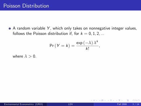
A random variable Y , which only takes on nonnegative integer values,follows the Poisson distribution if, for k = 0, 1, 2, ...
Pr (Y = k) =exp (�λ) λk
k !,
where λ > 0.
The mean and the variance of Poisson random variable is λ:
E (Y ) = Var (Y ) = λ.
Environmental Econometrics (GR03) LDV Fall 2008 3 / 14
Poisson Distribution
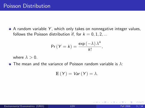
A random variable Y , which only takes on nonnegative integer values,follows the Poisson distribution if, for k = 0, 1, 2, ...
Pr (Y = k) =exp (�λ) λk
k !,
where λ > 0.
The mean and the variance of Poisson random variable is λ:
E (Y ) = Var (Y ) = λ.
Environmental Econometrics (GR03) LDV Fall 2008 3 / 14
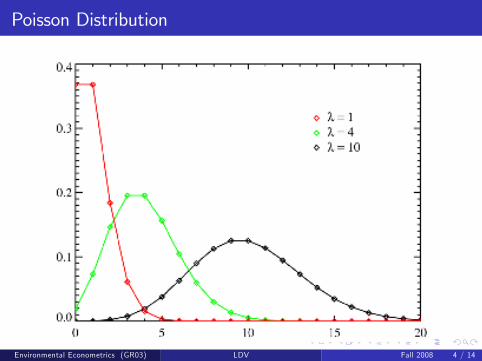
Poisson Distribution
Environmental Econometrics (GR03) LDV Fall 2008 4 / 14
Poisson Regression Model
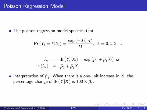
The poisson regression model speci�es that
Pr (Yi = k jXi ) =exp (�λi ) λki
k !, k = 0, 1, 2, ...
λi = E (Yi jXi ) = exp (β0 + β1Xi ) or
ln (λi ) = β0 + β1Xi
Interpretation of β1: When there is a one-unit increase in X , thepercentage change of E (Y jX ) is 100� β1.
Environmental Econometrics (GR03) LDV Fall 2008 5 / 14

Estimation
In principle, the Poisson model is simply a nonlinear regression. It ismuch easier to estimate the parameter with maximum likelihoodmethod.
The log-likelihood function is
ln L�
β0, β1; fYi ,XigNi=1
�=
N
∑i=1ln Pr (Yi = yi jXi )
=N
∑i=1[� exp (β0 + β1Xi ) + Yi (β0 + β1Xi )� ln(Yi !)]
Note that the Poisson model could be too restrictive since thevariance is equal to the mean.
Environmental Econometrics (GR03) LDV Fall 2008 6 / 14

Example: Number of Arrests
We apply the Poisson regression model for the number of arrestsduring 1986 in a group of men in California, USA.
The dependent variable is the number of times a man is arrested. Thefrequency of this variable is
# of times arrested0 1 2 3 4 5 � 6 Total
Freq 1970 559 121 42 12 13 8 2,725(%) (72.3) (20.5) (4.4) (1.5) (0.4) (0.5) (0.3) (100)
Environmental Econometrics (GR03) LDV Fall 2008 7 / 14
Example: Number of Arrests
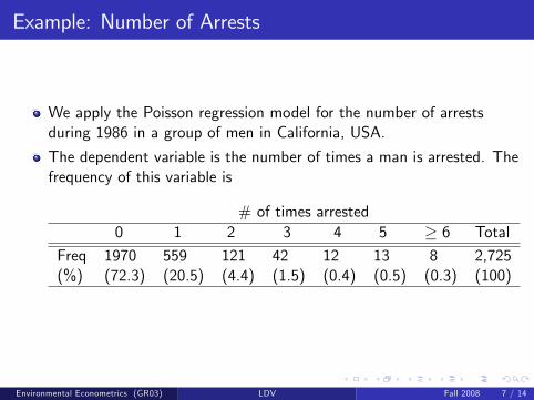
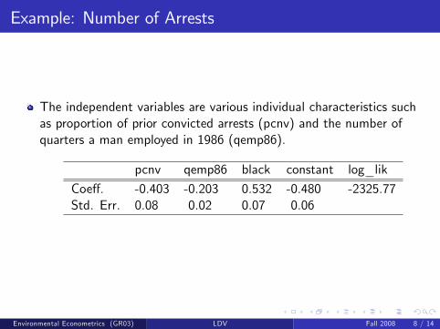
The independent variables are various individual characteristics suchas proportion of prior convicted arrests (pcnv) and the number ofquarters a man employed in 1986 (qemp86).
pcnv qemp86 black constant log_lik
Coe¤. -0.403 -0.203 0.532 -0.480 -2325.77Std. Err. 0.08 0.02 0.07 0.06
Environmental Econometrics (GR03) LDV Fall 2008 8 / 14
Models for Censored Data
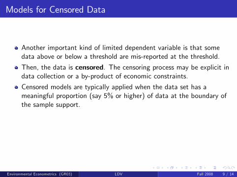
Another important kind of limited dependent variable is that somedata above or below a threshold are mis-reported at the threshold.
Then, the data is censored. The censoring process may be explicit indata collection or a by-product of economic constraints.
Censored models are typically applied when the data set has ameaningful proportion (say 5% or higher) of data at the boundary ofthe sample support.
Examples:
(corner solution) consumption of a good (smoking/alcohol);(data collection censoring) top-coding of income.
Environmental Econometrics (GR03) LDV Fall 2008 9 / 14

Models for Censored Data
Another important kind of limited dependent variable is that somedata above or below a threshold are mis-reported at the threshold.
Then, the data is censored. The censoring process may be explicit indata collection or a by-product of economic constraints.
Censored models are typically applied when the data set has ameaningful proportion (say 5% or higher) of data at the boundary ofthe sample support.
Examples:
(corner solution) consumption of a good (smoking/alcohol);(data collection censoring) top-coding of income.
Environmental Econometrics (GR03) LDV Fall 2008 9 / 14
Models for Censored Data
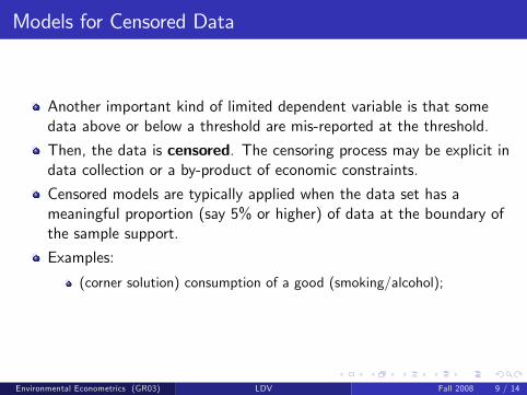
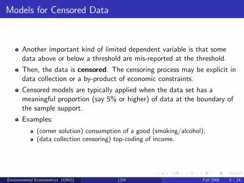
Another important kind of limited dependent variable is that somedata above or below a threshold are mis-reported at the threshold.
Then, the data is censored. The censoring process may be explicit indata collection or a by-product of economic constraints.
Censored models are typically applied when the data set has ameaningful proportion (say 5% or higher) of data at the boundary ofthe sample support.
Examples:
(corner solution) consumption of a good (smoking/alcohol);
(data collection censoring) top-coding of income.
Environmental Econometrics (GR03) LDV Fall 2008 9 / 14
Models for Censored Data
Another important kind of limited dependent variable is that somedata above or below a threshold are mis-reported at the threshold.
Then, the data is censored. The censoring process may be explicit indata collection or a by-product of economic constraints.
Censored models are typically applied when the data set has ameaningful proportion (say 5% or higher) of data at the boundary ofthe sample support.
Examples:
(corner solution) consumption of a good (smoking/alcohol);(data collection censoring) top-coding of income.
Environmental Econometrics (GR03) LDV Fall 2008 9 / 14

Structure of the Model
An underlying latent variable has the following relationship:
Y �i = β0 + β1Xi + ui , ui jX � N�0, σ2
�Yi =
�Y �i0
if Y �i > 0otherwise
The model is called Tobit. Then, the probability of censoring is given
Pr (Y = 0jX ) = Pr (Y � � 0jX )
= 1�Φ�
β0 + β1Xσ
�
Environmental Econometrics (GR03) LDV Fall 2008 10 / 14
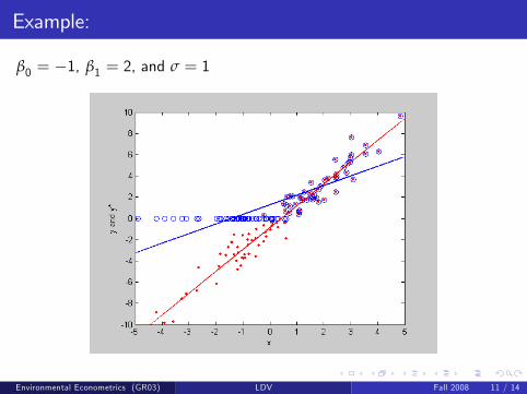
Example:
β0 = �1, β1 = 2, and σ = 1
Environmental Econometrics (GR03) LDV Fall 2008 11 / 14

Marginal E¤ects
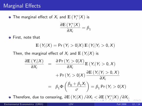
The marginal e¤ect of Xi and E (Y �i jX ) is∂E (Y �i jX )
∂Xi= β1
First, note that
E (Yi jX ) = Pr (Yi > 0jX )E (Yi jYi > 0,X )
Then, the marginal e¤ect of Xi and E (Yi jX ) is∂E (Yi jX )
∂Xi=
∂Pr (Yi > 0jX )∂Xi
E (Yi jYi > 0,X )
+Pr (Yi > 0jX )∂E (Yi jYi > 0,X )
∂Xi
= β1Φ�
β0 + β1Xiσ
�= β1 Pr (Yi > 0jX )
Therefore, due to censoring, ∂E (Yi jX ) /∂Xi < ∂E (Y �i jX ) /∂Xi .
Environmental Econometrics (GR03) LDV Fall 2008 12 / 14

Marginal E¤ects
The marginal e¤ect of Xi and E (Y �i jX ) is∂E (Y �i jX )
∂Xi= β1
First, note that
E (Yi jX ) = Pr (Yi > 0jX )E (Yi jYi > 0,X )
Then, the marginal e¤ect of Xi and E (Yi jX ) is∂E (Yi jX )
∂Xi=
∂Pr (Yi > 0jX )∂Xi
E (Yi jYi > 0,X )
+Pr (Yi > 0jX )∂E (Yi jYi > 0,X )
∂Xi
= β1Φ�
β0 + β1Xiσ
�= β1 Pr (Yi > 0jX )
Therefore, due to censoring, ∂E (Yi jX ) /∂Xi < ∂E (Y �i jX ) /∂Xi .
Environmental Econometrics (GR03) LDV Fall 2008 12 / 14

Estimation of Tobit Model
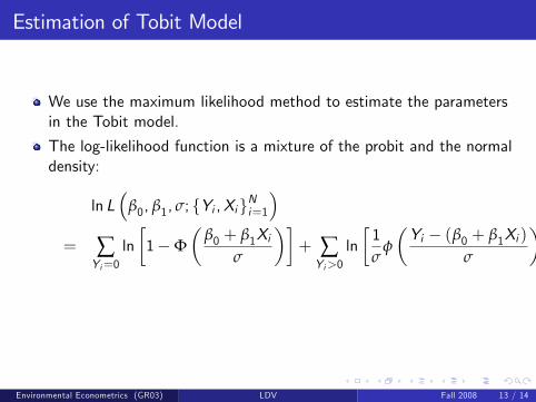
We use the maximum likelihood method to estimate the parametersin the Tobit model.
The log-likelihood function is a mixture of the probit and the normaldensity:
ln L�
β0, β1, σ; fYi ,XigNi=1
�= ∑
Yi=0
ln�1�Φ
�β0 + β1Xi
σ
��+ ∑Yi>0
ln�1σ
φ
�Yi � (β0 + β1Xi )
σ
��The ML estimators maximize the log-likelihood function with respectto the parameters.
Environmental Econometrics (GR03) LDV Fall 2008 13 / 14
Estimation of Tobit Model
We use the maximum likelihood method to estimate the parametersin the Tobit model.
The log-likelihood function is a mixture of the probit and the normaldensity:
ln L�
β0, β1, σ; fYi ,XigNi=1
�= ∑
Yi=0
ln�1�Φ
�β0 + β1Xi
σ
��+ ∑Yi>0
ln�1σ
φ
�Yi � (β0 + β1Xi )
σ
��
The ML estimators maximize the log-likelihood function with respectto the parameters.
Environmental Econometrics (GR03) LDV Fall 2008 13 / 14

Estimation of Tobit Model
We use the maximum likelihood method to estimate the parametersin the Tobit model.
The log-likelihood function is a mixture of the probit and the normaldensity:
ln L�
β0, β1, σ; fYi ,XigNi=1
�= ∑
Yi=0
ln�1�Φ
�β0 + β1Xi
σ
��+ ∑Yi>0
ln�1σ
φ
�Yi � (β0 + β1Xi )
σ
��The ML estimators maximize the log-likelihood function with respectto the parameters.
Environmental Econometrics (GR03) LDV Fall 2008 13 / 14
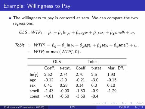
Example: Willingness to Pay
The willingness to pay is censored at zero. We can compare the tworegressions:
OLS : WTPi = β0 + β1 ln yi + β2agei + β3sexi + β4smelli + ui ,
Tobit : WTP�i = β0 + β1 ln yi + β2agei + β3sexi + β4smelli + ui ,
: WTPi = max (WTP�i , 0) .
OLS Tobit
Coe¤. t-stat. Coe¤. t-stat. Mar. E¤.
ln(y) 2.52 2.74 2.70 2.5 1.93age -0.12 -2.0 -0.21 -3.0 -0.15sex 0.41 0.28 0.14 0.0 0.10smell -1.43 -0.90 -1.80 -0.9 -1.29const -4.01 -0.50 -3.68 -0.4
Environmental Econometrics (GR03) LDV Fall 2008 14 / 14


