All rights reserved. No parts of this work may be reproduced in any form without the written permissionof LimitState Ltd.
While every precaution has been taken in the preparation of this document, LimitState Ltd assumes noresponsibility for errors or omissions. LimitState Ltd will not be liable for any loss or damage of anykind, including, without limitation, indirect or consequential loss (including loss of profits) arising out ofthe use of or inability to use this document and/or accompanying software for any reason.This document is provided as a guide to the use of the software. It is not a substitute for standardreferences or engineering knowledge. The user is assumed to be conversant with standardengineering terminology and codes of practice. It is the responsibility of the user to validate thesoftware for the applications for which it is to be used.
LimitState Ltd was spun out from the University of Sheffield in 2006 to develop and market cut-ting edge ultimate analysis and design software for engineering professionals. LimitState:SLABis one of a number of LimitState products, with applications in the structural, geotechnical andmechanical engineering sectors. We aim to be a world leading supplier of computational limitanalysis and design software. LimitState maintains close links with the University of Sheffield,enabling us to draw on and rapidly implement the latest innovations in numerical and theoreticallimit state analysis.
1.2 General Overview
1.2.1 LimitState:SLAB
LimitState:SLAB is a software program designed to rapidly evaluate the load carrying capacityof existing and proposed concrete slab structures using the yield-line analysis method.
Unlike many other analysis methods and tools, LimitState:SLAB uses modern optimizationtechniques to identify the most critical layout of yield-lines for the defined problem, removing theneed to propose a potential failure mechanism at the outset or manually refine the mechanismuntil an acceptable (and arbitrary) degree of accuracy is achieved.
LimitState:SLAB can be used to model problems of any geometry specified by the user, includ-ing those containing columns, walls and holes.
The software directly determines the ultimate limit state (ULS) collapse conditions using Dis-continuity Layout Optimization (DLO) (see Chapter II), and is designed to work with modernengineering design codes by providing full support for partial factors and the ability to solvemultiple load cases.
The yield-line method is a robust and powerful technique for estimating the ultimate capacity ofconcrete slabs. It is simple to understand, but also possesses the versatility to address a widerange of problem types. The method traditionally involves postulating a failure mechanism (oryield-line pattern) and then using work or equilibrium equations to calculate the loading requiredto cause collapse.
The method has a number of benefits, both when designing and assessing slab structures. Forcases of designing slabs, Kennedy & Goodchild (2004) identified the following when reviewingthe technique for a Concrete Centre design guide:
”Yield Line Design has the advantages of:
1. Economy
2. Simplicity
3. Versatility
Yield Line Design leads to slabs that are quick and easy to design, and are quickand easy to construct. [...]
The resulting slabs are thin and have very low amounts of reinforcement in veryregular arrangements. The reinforcement is therefore easy to detail and easy to fixand the slabs are very quick to construct.
Above all, Yield Line Design generates very economic concrete slabs, because itconsiders features at the ultimate limit state. [...]”
It naturally follows that, for the assessment of existing slab structures, the Yield-Line methodwill be able to highlight inherent strength in slabs that may not have been considered duringthe design stage. This makes it an ideal tool when repurposing a building with contents thatsurpass the initial design loading.
However, Kennedy & Goodchild (2004) note that:
”...a traditional and legitimate concern has been that an overestimate of the true ca-pacity will be obtained unless the correct collapse mechanism has been identified.”
An automated method capable of reliably and systematically identifying critical yield-line pat-terns, as highlighted above, has long been sought and various methods have previously beenput forward (e.g. Munro & Da Fonseca 1978, Johnson 1994, etc.). However, none of thesemethods have been sufficiently capable enough to find widespread application in engineeringpractice.
LimitState:SLAB solves these problems by using state-of-the-art optimization techniques (DLO)to identify, for any particular problem, the critical layout of yield-lines and therefore provide avery close upper bound on the true solution.
The Discontinuity Layout Optimization (DLO) procedure (originally introduced in Smith & Gilbert2007) provides a simple yet systematic and completely general means of identifying criticalcollapse mechanisms in plastic analysis problems. LimitState:SLAB harnesses the power ofthis procedure in a simple-to-use yet powerful software product. The application of DLO toyield-line analysis is outlined in Gilbert et al. 2014.
More information about the DLO procedure is also given in Chapter II
1.3 Program Features
LimitState:SLAB is designed to be general, fast and easy to use. The main features of Limit-State:SLAB are summarized below:
• LimitState:SLAB utilizes Discontinuity Layout Optimization (DLO) to directly identify thecritical yield-line collapse mechanism. The DLO procedure effectively relies on the fa-miliar ‘mechanism’ method of analysis originally pioneered for slabs by workers such asJohansen (1962), but posed in a modified form to allow modern-day computational powerto be applied to the problem of finding the critical solution from billions of possibilities.
• The solution is presented as an ‘adequacy factor’ (applied to one or more loads in theproblem) and also displayed visually as a failure mechanism involving a number of solidelements which will rotate relative to one another. To facilitate rapid interpretation of themode of response the failure mechanism can be animated.
• Many types of problems can be solved, including those involving walls, columns, holesand areas of differing thickness. The problem geometry can be specified using Wizardsfor common problems or alternatively by:
– drawing the geometry on-screen using the mouse,
– importing from a CAD (DXF) file.
The geometry can subsequently be edited using the mouse or by editing coordinates.
• All Materials and reinforcement patterns are available by applying specified Mp values,(the user inputs pre-calculated moment capacity values for hogging and sagging in twodirections). Orthotropic and skew reinforcement can be easily incorporated.
• LimitState:SLAB provides extensive support to users wishing to use Partial Factors:
– user specified partial factor sets can be defined,
– different partial factors can be defined for permanent, variable, accidental and favourableor unfavourable loads,
• LimitState:SLAB provides a comprehensive and easy to use GUI interface with fully se-lectable geometry objects, a Property Editor, Materials Explorer, Loads Explorer and dragand drop facilities. It also provides users with full Undo/Redo facilities and ability to re-cover lost work via an auto-saved recovery file.
• A comprehensive Report can be generated, with user control over what is included, andthe unique ability to output free body diagrams for all solid elements which define thecritical failure mechanism, with equilibrium equations to permit easy hand validation.
• Comprehensive guidance within the program in the form of messages, warnings and textdescriptions. Where appropriate these are hyperlinked direct to relevant sections withinthe online help file.
• Choice of working in Metric or Imperial units.
1.4 LimitState:SLAB Terminology
LimitState:SLAB is designed to rapidly identify the critical failure mechanism in any concreteslab analysis problem. The following annotated image highlights the most important on-screenentities the user will encounter when using LimitState:SLAB:
Figure 1.1: The main user interface objects in LimitState:SLAB
1.5 Using Help
Pressing F1 at any time gives users access to the online help facility, providing users with aconvenient means of accessing material contained within the manual whilst using the software.The software also includes hyperlinks which link directly to relevant parts of the online help
material (e.g. from within messages, dialogs and text descriptions), to provide users with rapidaccess to relevant explanatory material.
1.6 System Requirements
LimitState:SLAB runs on the Windows XP, Windows Vista and Windows 7 operating systems(support for Mac OSX and Linux operating systems is available on request, subject to demand).Recommended minimum system specifications are as follows (ideal values are given in paren-thesis):
The program uses a ‘Single Document Interface’ which means that one project file can be openin LimitState:SLAB at any given time. However, several instances of LimitState:SLAB can beopened simultaneously if required and each of these may contain a separate project file.
When using LimitState:SLAB with a ‘full’ license, problem size is limited only by available com-puter power.
1.8 Platform Limitations
1.8.1 Macintosh
The following are known limitations, or differences in behaviour, when being run on a Macintoshcomputer:
• Licenses tied to a USB dongle are not available (no supporting drivers).
• Animations cannot be exported to AVI.
• The colour palette does not contain a range of pre-defined colours.
• The layout of buttons is in Windows format (i.e. ‘OK - Cancel’ rather than ‘Cancel - OK’).
• Full screen mode is not supported.
• Hiding toolbars may cause white ‘shadows’ to be rendered at the top of the screen.
To request information on pricing, a formal quotation, or to purchase the software please contactLimitState Ltd, at [email protected].
1.9.2 Software Support
Software support for LimitState:SLAB is available to all users with a valid support and mainte-nance contract. Additionally we are happy to help users with time-limited ‘trial’ or ‘evaluation’licenses. All queries should be directed to [email protected].
1.9.3 Website
For the most up-to-date news about LimitState:SLAB, please visit the LimitState:SLAB website:www.limitstate.com/slab.
Details relating to the installation and licensing of LimitState software are provided in the sepa-rate ‘Installation and Licensing Guide’.
2.1.1 Thumbnails, Tags and File Search
For users running Windows 7 or above, the ability to include thumbnails and tags with the savedproject is available1. Careful use of these features allows different LimitState:SLAB files to becategorized and later searched for on a computer, without the need to open and inspect eachone individually. Additionally, other properties from the Project details dialog can be searchedif the system properties are set appropriately.
2.1.1.1 Enabling Thumbnails
To allow a system to take advantage of the thumbnail feature it may be necessary to set it todisplay these instead of the program icon. To do this:
1. Open Control Panel on the PC.
2. Select Folder Options.
3. Select the View tab.
4. Ensure that Always show icons, never thumbnails is NOT selected.
5. Click OK.
For further information see Chapter 10. Note that uninstalling LimitState:SLAB may require areboot to remove the thumbnails feature from Windows registry.
1For Windows Vista users, thumbnails may be available depending on the system configuration.
19
20 CHAPTER 2. GETTING STARTED
2.1.1.2 Enabling File Property Searching
To allow a system to search within the Project details it may be necessary to change thedefault search settings. To do this:
1. Open Control Panel on the PC.
2. Select Folder Options.
3. Select the Search tab.
4. Ensure that Always search file names and contents... IS selected.
5. Click OK.
For further information see Chapter 10. Note that searching for file properties in a folder thatis included in the Windows ”Index” may not work at first. This is because the system requirestime to register the file properties in the index and, during this period, will not return matches.The expected behaviour will return once indexing has occurred.
2.2 Starting LimitState:SLAB
To start LimitState:SLAB, on the Start menu, point to All Programs, then click on Limit-State:SLAB. On starting LimitState:SLAB the following welcome screen should appear (Figure2.1).
Figure 2.1: LimitState:SLAB welcome screen
Users then have three options:
1. Create a new project - select this option and click OK to bring up the New Project Dia-log. You may then select either an ‘Empty project’ (which provides you with full flexibility
to define the geometry of your problem), or one of the application-specific predefinedprojects, each of which will activate a wizard to guide you through the process of specify-ing your problem.
2. Open an existing project - select this option and click OK to display the open file dialog.
3. Open a recently accessed project - select this option, choose a file from the list andclick OK to return to a recent project.
2.3 The Adequacy Factor
In order to drive a problem to failure, LimitState:SLAB must increase one or more loads to sucha magnitude that the moment resistance provided by the slab is surpassed in enough locationsto form a mechanism (i.e. a collapse state). The user determines which loads are increased inthe analysis by setting the Adequacy property to True. Upon solve, the optimization processdetermines the lowest multiplier on these loads required to cause collapse. This multiplier iscalled the Adequacy factor.
The Adequacy factor can be interpreted in two different ways, depending upon the PartialFactors that have been set:
1. Unit Partial Factors
When all Partial Factors are set to 1.0 (Unity), the Adequacy factor reported is a ba-sic multiplier on the applied loading.
For example, if a pressure load of 1kN/m2 is applied and the Adequacy factor re-ported is 3.1, a total pressure load of 3.1kN/m2 is required to cause collapse.
2. Non-Unit Partial Factors
When any Partial Factors are non-unit (i.e. not 1.0), the loads and / or material prop-erties are factored in advance of the analysis. Therefore, the Adequacy factor reported mustbe greater than, or equal to, 1.0 in order for the system to be deemed ‘safe’.
More about the Adequacy factor is given in Section 6.2.
2.4 Guidance Available in this Manual
Guidance is available as follows:
1. For a Quick Start introduction to LimitState:SLAB refer to Chapter 3.
2. For a description of the theory underlying the solutions generated by LimitState:SLABrefer to the Theory chapters in Part II.
This chapter is designed to provide users with an overview of the capabilities of LimitState:SLAB.It is recommended reading for new users and will prepare them to subsequently make use ofsome of the more sophisticated features of the program.
For the sake of brevity some topics are not discussed in depth in this chapter. For furtherinformation on all topics, the reader is referred to the Modelling Guide (Part III) and User Guide(Part IV).
3.2 Overview of the Modelling and Analysis Process
When starting to model a problem using LimitState:SLAB the option is either:
1. To use a built-in ‘Wizard’ to quickly define a basic problem, or
2. To build a model from scratch, using a geometry imported from a DXF file or drawn byhand.
The process involved in either case follows the outline below:
i) Define geometry.
ii) Assign support conditions.
iii) Assign material properties.
iv) Define loading.
v) Set up load cases and partial factor sets.
vi) Analyse.
vii) Query post-solve information.
23
24 CHAPTER 3. QUICK START TUTORIAL
3.3 Getting Started
The following section describes how to set up and solve a problem in LimitState:SLAB. Usersshould follow instructions marked with a � symbol. Note that the values assume that the useris working in metric units. Results may differ if using Imperial units.
It is assumed that the user is starting from the Welcome to LimitState:SLAB dialog.
Create a New Project:
� Select Create a new project and click OK to bring up the New Project dialog, (see Figure3.1).
Figure 3.1: The LimitState:SLAB New Project dialog
If Cancel is selected, the user is free to define their own problem geometry. Alternatively, use ofa wizard permits rapid definition of common problem geometries. The geometry can be easilyamended subsequently.
3.3.1 Slab Geometry
� Select Empty and click OK.
The Empty Project Wizard then appears. Project data is entered in two stages as follows (theicons in the navigation bar on the left hand side of the wizard will be highlighted during eachstage of the problem definition):
Project Background details to the project may be entered here.
Figure 3.3: A square slab, specified using the ‘Draw Rectangle’ functionality.
Modify the Slab:
� Draw another rectangle, this time from (2, 3) to (3, 4).
� Click in the smaller square zone that is created (it will turn pink when selected).
� Press DELETE on the keyboard (alternatively, click the icon in the top toolbar). Thesmall square will now be removed from the problem as shown in Figure 3.4.
Figure 3.4: Remove a section of the slab, also using the ‘Draw Rectangle’ functionality.
3.3.2 Boundary Conditions
3.3.2.1 External Boundaries
External boundaries in LimitState:SLAB can take one of the following forms:
Free The boundary is free to displace and / or rotate in any direction.
Simple The boundary is fixed against displacements in all directions. Rotations of the slabaround the axis of the boundary are permitted without yield-line formation.
Fixed The boundary is fixed against displacements in all directions. Rotations of the slabaround the axis of the boundary are only permitted as a result of yield-line formation.
Partially Fixed The boundary is fixed against displacements in all directions. Rotations of theslab around the axis of the boundary are only permitted as a result of yield-line formationat a moment equal to the specified ratio multiplied by the strength of the adjacent slab.
Symmetry The boundary represents a line of symmetry in the model.
3.3.2.2 Internal Boundaries
Internal boundaries in LimitState:SLAB can take one of the following forms:
Free The boundary is free to displace and / or rotate in any direction.
Knife-edge The boundary is fixed against displacements in all directions. Rotations of the slabaround the axis of the boundary are permitted without yield-line formation.
3.3.2.3 Lift-off
In certain circumstances it may be desirable to allow a slab to be supported from vertical down-wards displacement, but for it to be able to move vertically upwards. By setting the Supportlift-off field to true, LimitState:SLAB will permit this to occur.
Note that lift-off can only be specified for the following boundary types:
• Simple (external boundary)
• Knife-edge (internal boundary)
Set the Boundary Conditions:
� Ensure that Click Select is active (select the and icons).
� Hold down CTRL on the keyboard and click the left, bottom and right Boundaries (thesewill be highlighted pink once selected).
� In the Property Editor (at the right of the screen), the dropdown will read ‘External Bound-aries (3)’. Double-click the Value field corresponding to the Support Type and select Fixedfrom the dropdown menu that appears.
� Click in the Viewer Window. The previously selected boundaries will now be fixed. Thisis denoted by cross-hatching (Figure 3.5).
Figure 3.5: Cross-hatching along a boundary signifies a fixed boundary condition. Rotationsalong the axis of the boundary are only permitted as a result of yield-line formation.
3.3.3 Slab Definitions
Slab Definitions define the unit weight, thickness and moment resistance of a slab and can beassigned on a per-zone basis:
Name / ID A unique identifier / name
Color The color as displayed on screen
Unit Weight The unit weight of the slab in any area where this definition is applied
Thickness The thickness of the slab in any area where this definition is applied
Mp The plastic moment of resistance per unit length. To allow for the presence of skewed andorthotropic reinforcement, this is split into two directions named First and Second . Thefollowing may then be defined for each:
• Mp+, The sagging plastic moment of resistance in the direction specified by theAngle.
• Mp−, The hogging plastic moment of resistance in the direction specified by theAngle.
• Angle (o), The angle (anticlockwise) described between the global x axis and thedirection in which Mp is acting. Note that this is NOT the angle of the reinforcing bars(α in Figure 3.6), rather it is the angle NORMAL to them (β in Figure 3.6).
By default, newly generated solid zones are not assigned any Slab Definition.
Built-in Slab Definitions are identified by the presence of a lock on their icon. The values ofthe attributes in a locked structural property cannot be changed. However, new slab definitionscan be generated and assigned to zones in place of the default.
Add a New Slab Definition:
� Right-click in the Slab Definitions Explorer and select New slab definition from the contextmenu that is displayed.
� Ensure Flexural is selected in the Type dropdown.
� Name the slab definition ”Example Material” and provide a color
� Set the slab properties to be:
• Unit weight = 0.0 (i.e. assume it is weightless)
• Thickess = 1.0 (default value)
• First direction:
– Mp+ = 1.0
– Mp− = 0.5
– Angle = 0 degrees
• Second direction:
– Mp+ = 2.0
– Mp− = 1.0
– Angle = 90 degrees
� Click OK .
Assign the New Slab Definition:
� In the Slab Definition Explorer, click and hold on the newly generated slab property.
� Drag the newly generated Slab Definition over to the slab in the Viewer Window and re-lease the mouse button.
� The zone will now be assigned the new Slab Definition (the color will change).
Note that you can also change the Slab Definition assigned to a zone via the Property Editor.
3.3.4 Loading
Loading in LimitState:SLAB can take the form of:
Point Loads A single load applied at a specified location.
Line Loads A uniform load (i.e. load per unit length) applied between two specified locations.
Pressure Loads A uniform pressure load (i.e. load per unit area) applied to one or more spec-ified solid zones within the problem.
Self-weight Loads Pressure loads resulting from the unit-weight and thickness of the slab.These can be applied on a per-zone basis.
3.3.4.1 Load Types
Loads (or actions) in LimitState:SLAB are assumed to take one of three Types, to which partialfactors can be applied. These relate to the amount of time that the load is anticipated to be incontact with the structure and correspond to classifications common to many codes of practice,such as the Eurocodes:
Permanent A load or action that is expected to remain on the structure indefinitely (i.e. bepersistent).
Variable A load that is expected to exist temporarily at the specified location on the structure.
Accidental A load that is expected to occur only in rare or exceptional circumstances.
3.3.4.2 Adding a Load
Adding loads to a problem requires two things:
1. Loads must be defined (in terms of magnitude and type) and added to the Loads Database.
2. Load Cases must be defined. This is done by selecting predefined loads from the LoadsDatabase and applying them at specified locations in the model along with specifiedpartial factors and other case-specific options.
LimitState:SLAB allows the user to define and copy loads across load cases using the LoadCase Manager. Alternatively, a quicker option (for instances where the loading is relativelysimple) is to use one of the loading icons in the user interface:
Point Load Add a point load at a specified location.
Line Load Add a line load between two specified points.
Pressure Load Add a pressure load to one or more zones.
Using this method, a load can be defined and added to both the Loads Database and thecurrent Load Case in a single action.
Add a Point Load:
� Click the Point Load icon, .
� Hover the pointer over the slab at position (3, 2) and click. This will bring up the Add NewLoad dialog (Figure 3.7).
� Choose Use existing Unit point (load) and confirm that the load position is correct. Leave theAction Type and Adequacy as their default values.
� Click OK . A point load will now be created and displayed at location (3,2) (Figure 3.8). Notethat, by default, all partial factors on load and material strengths are set to unity. To change this,open the Load Case Manager (via the menu item Loads). Here, existing or new partial factorsets can be assigned as necessary. For the purposes of this example the default settings willbe used.
Figure 3.7: Adding a new (unit) point load to the model.
Figure 3.8: A point load displayed on the model at location (3,2).
3.3.5 Solving the Problem
The problem is now ready to be solved.
In order to analyse the ultimate limit state, at least one load in the problem must be increaseduntil the collapse state is reached. In order to indicate to LimitState:SLAB which load this isto be, the Adequacy property must be set for at least one load. In this case the wizard hasautomatically set the Adequacy property for the point load applied to the slab. The returnedAdequacy Factor is the factor by which that load must be increased in order to cause collapse.For further information on the Adequacy factor and its usage, see Section 6.2.
When the load was added (Section 3.3.4.2), the Adequacy variable was set to True. Thismeans that the point load is subject to factoring during the analysis. (Note that any otherloading with Adequacy=True would also be factored during solve).
There are three methods by which the analysis can be triggered:
1. Go to the Analysis menu and select Solve.
2. Press F5.
3. Click the icon.
Solve:
� Using one of the methods described, solve the problem.
The program will first display a series of nodes, superimposed on the geometry objects in theproblem, and will then rapidly try out all possible combinations of yield-lines interconnecting thenodes to find the optimum solution. The program will gradually refine the failure mechanism untilan optimal yield-line mechanism is found (Figure 3.9), together with an associated Adequacyfactor (margin of safety) on the specified load.
Figure 3.9: Slab problem displayed in the main viewer (after analysis and before animation).
In the solution, red yield-lines denote failure by hogging and blue yield-lines represent failurein sagging. The thickness of the lines indicates the magnitude of the rotation, allowing thedominant failure mechanism to be clearly identified.
With the specified parameters, an Adequacy factor of 13.03 should be obtained (displayedin the Output window at the bottom of the screen). This means that the slab is safe againstcollapse until the point load has increased by a factor of approximately 13.03. As the probleminvolves unit partial factors, the Adequacy factor is a direct multiplier on the applied load.
In general, when non-unit partial safety factors are applied in the problem:
• Adequacy factor > 1.0, the problem is safe against collapse
• Adequacy factor < 1.0, the problem is unsafe against collapse.
3.4 Viewing Mechanism Deformation
By default the software will automatically animate the solution after solve (Figure 3.10), by mag-nifying the instantaneous displacements at failure. Note that although the solution is strictly only
valid for infinitesimal displacements, large displacements are displayed to assist visualizationof the collapse mode. For direct control over magnification of the mechanism displacements,
the slider bar can also be used. The Play Animation button can be clicked toreplay the animation.
Figure 3.10: 3D Deformation of the Quick Start Slab problem.
3.5 Viewing Post-Solve Information
Following analysis, a number of post-solve information becomes available to the user:
3.5.1 Yield-Lines
By clicking on an individual yield-line, the following information is shown in the Property Editor:
ID The name of the yield-line.
Start node Coordinates of the start of the yield-line.
End node Coordinates of the end of the yield-line.
Length The length of the yield-line.
Moment The moment experienced at the yield-line.
Rotation The instantaneous relative rotation along the yield-line.
� Click on any yield-line in the solved problem - inspect the available data in the PropertyEditor.
After the software has solved a problem, the user is able to select any of the solids defining thefailure mechanism (by clicking with the mouse). This will display a diagram of the bending mo-ments acting around the edges of the selected object. Hovering over each part of the diagramwill display the magnitude of the moment next to the mouse cursor.
3.6 Zooming In and Out
To zoom in and out, use the magnifying glass toolbar buttons (Zoom In , Zoom Out ,
Zoom All ), or, if a scroll wheel mouse is being used, use the wheel to zoom in and out. Notethat with the mouse, zooming takes place centred on the current position of the mouse pointer
(the Select button must be on for this feature to work). Zoom All resizes the image to displayoptimally in the viewer. This is useful if the image has become too large or small.
3.7 Pan, Rotate and 3D Views
To pan, select the cross arrows toolbar button ( ) and hold the left mouse button while drag-ging inside the Viewer Pane. Alternatively, if a scroll wheel / 3 button mouse is being used,click and hold the central button. The arrow keys on the keyboard will also change the view.Note that panning takes place centred on the current position of the mouse pointer.
To rotate the view in 3D, select the rotate toolbar button ( ) and hold the left mouse buttonwhilst moving the cursor in the Viewer Pane. To return the view back to the default, right-clickin the Viewer Pane to bring up the context menu. From here, select View >Front to return thedisplay to the default viewing angle. Using the context menu, or the View 3D toolbar (AppendixB.3.2), it is also possible to snap the viewer to a number of pre-defined 3D viewing angles.These can be particularly effective when examining the solved problem.
3.8 Trying Different Problems and Parameter Sets
Modifications can be made to an existing project via the Property Editor and the solution canthen be recalculated to reflect the changes.
Note that if there is a previously solved problem, the Unlock icon must be clicked to allowmodification of any of the parameters; this is to prevent inadvertent alterations being madeonce a solution has been obtained.
To generate a new problem, click File>New or and select a wizard or Empty project.
The Property Editor (PE), displayed on the right hand side of the display, allows the user toquickly read and / or modify the attributes of one or more objects within the current project.Figure 3.11 shows the typical parameters displayed in the Property Editor when a Solid Objectis selected.
Figure 3.11: Parameters displayed in the LimitState:SLAB Property Editor when a Solid Objectis selected.
Some of the functions in LimitState:SLAB are only accessible via the Property Editor. Theseare described in more detail in this section. Other functions and attributes can be accessedand modified elsewhere, but are shown for convenience in the PE.
Generally, when an object is selected, it will be highlighted and its properties will be displayedin the PE. Single clicking on any item in the Property column gives an expanded explanation
of the parameter in the window at the base of the PE. A sign next to an item indicates that
there are additional sub-parameters relating to that item that may be viewed. Click on thesign to access these. Clicking on a value in the PE allows it to be modified by typing or selectingthe required choice, unless it is a read only value or the project is Locked.
By default the Slab Definition Explorer is located on the left hand side of the screen. Thiscontains a list of available slab definitions.
Note that any system defined slab definitions (indicated by a padlock symbol: ) are readonly and may not be changed. User-editable copies may however be made or new definitionscreated as follows:
� Right-click on the ”Unit MP Weightless” icon and select Duplicate slab definition. Click thenewly created definition (named ”Copy of Unit MP Weightless”) to view the properties in theProperty Editor.
� Change the name of the definition and the color of the material.
� Change the values of one or more moment capacities. To do this, click on the field containingthe value, enter a new value then press Enter or click elsewhere in the Property Editor toaccept the value).
3.9.2 Changing the Slab Definition(s) Used in a Solid Object
� Unlock the problem and click anywhere in the slab solid in the viewer (to use single selection,
ensure that toolbar buttons and are set to On).
Figure 3.12: Problem geometry with slab solid highlighted following selection.
Once selected, the Solid Object representing the slab will be highlighted in pink (as shown inFigure 3.12), and its properties displayed in the Property Editor. To change the allocated slabdefinition, three options are available:
1. If a Slab Definition defined by the user (manually or in a wizard) has been selected,its properties may be freely edited directly in the PE in the same way as described in
Section 3.9.1. (It is necessary to click the sign next to the Slab Definition caption inthe Property column of the PE to access the properties.)
2. If it is necessary to allocate an existing Slab Definition to the Solid Object representingthe slab, ‘drag and drop’ may be used. Using the mouse, drag a structural object fromthe Slab Definition Explorer onto the Solid Object representing the slab. A dialog boxwill be displayed and the user asked whether the Slab Definition is to be replaced. ClickReplace and the new structural object will be used in place of the previous one. Thecolour of the solid object should change to reflect the change in structural object (this willnot be seen while the slab is still selected).
� Replace the default slab definition with the new slab definition made previously.After solving, the computed Adequacy Factor should have changed.
3. The third option, which is an alternative to drag and drop, is to click on the Value cellin the Slab Definition row in the PE (this should say ‘1 slab definition assigned...’). AChange button will appear. Click this and the Edit Slab Definitions(s) dialog will allowthe selection of a slab definition (or set of slab definitions) that can be used in the slabsolid.
3.9.3 Resizing a Solid
Changing the geometry of a problem is straightforward. Simply click on a Vertex of the slaband, with the left hand mouse button held down, drag this Vertex to a new location.
Figure 3.13: Moving a vertex by clicking and dragging in the viewer
3.9.4 Changing the Slab Definition Used on a Boundary
The Slab definition used on a boundary can be changed in one of two ways:
1. Click on a Slab definition from the Slab Definitions Explorer. With the left mousebutton held down, drag the chosen definition over the boundary that you wish to modify.The boundary will turn pink. At this point, release the mouse button. The definition will beapplied or, if a definition is already present on the boundary, a prompt will be displayed,asking if you wish to replace the existing definition.
2. Select one or more boundaries using the mouse (hold CTRL or use the Rectangle selectfor multi-selection). In the Property Editor, click the right-hand field next to the SlabDefinition and select the Change... button that appears. A dialog will be shown (asdepicted in Figure 3.14) which allows you to change the definition.
Figure 3.14: Changing the Slab Definition used on a Boundary
3.9.5 Modifying Loads
Loads in LimitState:SLAB are defined via the Loads Database and the Load Case Manager.Refer to Chapter 17 for more information on how to work with loads.
3.10 Solution Accuracy
As with most numerical methods, solution accuracy is governed by the numerical discretizationused in the underlying model.
With DLO the numerical discretization is controlled by the distribution of nodes within Solid andBoundary objects. Using the DLO procedure, the most critical mechanism that can be identi-fied from the set of all potential yield-lines which interconnect these nodes is identified. In many
cases a sufficiently accurate solution will be generated when a relatively coarse distribution ofnodes is employed.
The number of nodes to be used can be controlled via the Nodal Density setting, accessiblevia the Property Editor under ‘Project’. The basic settings are Coarse, Medium, Fine andVery Fine. To investigate the effect of nodal distribution on the problem in Section 3.3.5, set upa new problem. Solve and note the solution then click anywhere in an empty part of the Viewerpane (the part of the screen where the problem geometry is displayed). This will display theproject level properties in the Property Editor. Change the value in the Nodal Density entryto Fine, and then solve the problem again. This time a similar but more detailed collapsemechanism is found and the associated adequacy factor is slightly lower.
Figure 3.15: Simple Slab critical yield-line pattern (after analysis with a Fine nodal resolution)
3.11 Conclusion
This brief quick start tutorial has been designed to familiarize users with the basic functionalityof LimitState:SLAB. It is recommended that users experiment with the various wizards, andmodify the parameters involved, before constructing problems from scratch.
LimitState:SLAB provides a number of Wizards which allow the user to rapidly create modelsof commonly encountered problems. Variants on these geometries are easily generated bymodifying the basic geometry created by the Wizard (see Section 14.6). To use a Wizard,select Create a new project in the Welcome to LimitState:SLABdialog and click OK , or, if
the software is already running then click File>New or . The New Project dialog (Figure4.1) will then start.
A number of different project types are available, all of which initiate a Wizard.
Figure 4.1: The New Project dialog
Empty Creates an empty project for the user to draw their own model. This includes optionsfor specifying an underlying grid. It solves for the factor on applied loads.
Rectangular Slab Creates a model of a basic (skewed) rectangular slab. The default loadingis set to vertical with a unit pressure.
43
44 CHAPTER 4. WIZARDS
Rectangular Slab With Hole Creates a model of a basic (skewed) rectangular slab with ahole. The default loading is set to vertical with a unit pressure.
Select the required Project Wizard and click OK .
4.2 Using a New Project Wizard
4.2.1 Introduction
The Wizards in LimitState:SLAB are designed to help the user quickly generate a model of theirproblem.
Each Wizard guides the user through the process of defining the model:
• Project description (Section 4.2.2)
• Geometry (Section 4.2.3)
• Slab Definitions (Section 4.2.4),
• Loads (Section 4.2.5)
• Analysis (Section 4.2.6)
It should be noted that, at any point whilst running a Wizard, it is possible to click Finish.LimitState:SLAB will automatically fill in any information that has not been explicitly supplied(by using default values together with information already provided by the user up until thatpoint).
In most cases, information is entered in a sequential manner, the user clicking Next after eachstep. However, it is possible to move backwards through the various steps by using the Backbutton. The left-hand pane of the Wizard dialog serves as a reference point, with the currentsection being highlighted in blue as shown for the Project description stage in Figure 4.2.
All parameters with dimensions should be entered in either Metric or Imperial units dependingon the program preferences set by the user (see Section 13.1). When a data entry box is
selected, data entry via a calculator is also available by clicking on the calculator button .The Calculator (see Section 8.10) also incorporates a unit converter for many commonly usedunits, including Metric and Imperial units.
4.2.2 General Project Settings
This dialog allows entry of the Project name, Reference number , Location, Engineer name,Organization, general Comments and Tags. This information may be included in the Reportoutput (Section 20). For further details on the Tags functionality, see Chapter 10.
4.2.3 Geometry
The next stage is to describe the geometry of the problem. Figures in the dialog clearly indicatethe meaning of the parameters to be entered, e.g. as shown in Figure 4.3.
The geometry data entry is normally designed to prevent unrealistic/impossible geometriesbeing entered. However this is not feasible in all cases. If a combination of parameters isentered that would result in an unrealistic geometry being generated, a warning message willbe displayed on pressing Finish and the software will adjust the geometry to produce a fea-sible result. The user may then either edit the final geometry directly (see Section 14.6), or,alternatively re-run the wizard.
4.2.4 Slab Definitions
Each tab in this dialog allows the user to specify the basic properties of the materials used inthe problem or to select a material from a predefined list as shown in Figure 4.4.
In order to keep the Wizards straightforward to use, only basic material properties are entered,and default values are used for the other properties. To edit other available properties it isnecessary to use the Property Editor once the Wizard has been exited.
4.2.5 Loads
Specify the required loads here as shown in Figure 4.5. Loads will generally by default have amargin of safety or Adequacy factor computed for them. For such loads, you may either enterthe actual applied load and a margin of safety will be computed. Alternatively a value of 1.0may be entered and the Adequacy factor will equal the collapse load. For further discussionof the Adequacy factor see Chapter 17.
This stage displays the Analysis tab, as shown in Figure 4.6. Here the user can alter the nodaldensity of the problem.
By default the Nodal Density is set to Medium (500 nodes). The Target Number field willdisplay the number of nodes associated with the selected density and, when a custom densityis specified, the value can be set manually.
Figure 4.6: A typical Wizard analysis options dialog
The yield-line method is a long established, highly effective and widely used means of estimat-ing the ultimate load carrying capacity of concrete slabs. The method was originally developedby Ingerslev (1923) and subsequently significantly enhanced by Johansen (1962). The upperbound status of the method within the context of the then emerging plastic theories of structuralanalysis was later confirmed by others (e.g. see Save et al. 1997). The method traditionallyinvolves postulating a collapse mechanism which is compatible with the boundary conditionsand then using equilibrium or the principle of virtual work to compute the ultimate load, or ‘loadfactor’.
For certain special cases it has been possible to calculate provably exact failure load factors(e.g. by Fox 1974 for a uniformly loaded fixed square slab). However, in the case of mostreal-world geometrical configurations (for example slabs containing columns, holes etc), exactload factors are not available. In such cases unless the critical yield-line pattern is found,the computed load factor will over-estimate the true load factor. Whilst lower-bound methodscan be used to bound the load factor from below, the gap between a yield-line solution and asolution obtained using common lower bound analysis methods (e.g. the strip method proposedby Hillerborg (1975), which simplifies the problem by allowing analyst/designer to select loadpaths whilst ignoring twisting moments) will typically be found to be quite wide. This situationis clearly unsatisfactory and has undoubtedly limited the extent to which hand-based yield-lineanalysis has been used in practice.
Consequently various computational methods have been applied to the problem over the pastfew decades. For example, rigid-plastic finite-elements were investigated in the context of re-inforced concrete (RC) slab analysis by Anderheggen & Knopfel (1972). Their lower-boundmethod involved linearizing the yield function. More recently Krabbenhoft & Damkilde (2003)demonstrated that by using appropriate element formulations, and harnessing modern compu-tational resources, that good lower bound approximations could be obtained using rigid-plasticfinite elements. However, such rigid-plastic methods have not found their way into routine en-gineering practice and engineers typically instead have to rely on potentially cumbersome iter-ative elasto-plastic analysis methods. Furthermore, since finite element analysis is concernedwith treatment of an underlying continuum mechanics problem, such methods do not explicitlyidentify patterns of yield-lines (though in many cases these may subsequently be inferred from
51
52 CHAPTER 5. COMPUTATIONAL YIELD-LINE ANALYSIS
the output).
To address this, computational methods which explicitly identify yield-lines have also been de-veloped in parallel. For example, Chan (1972), and later workers such as Munro & Da Fonseca(1978) and Balasubramanyam & Kalyanaraman (1988), proposed methods in which potentialyield-lines were placed at the boundaries of rigid elements in a finite element mesh. This per-mits LP to then be used to identify the most critical arrangement of yield-lines. Whilst availablecomputing resources of the time meant that only relatively coarse meshes could be treated,the more significant problem with such methods is sensitivity of the results to the chosen meshlayout, with the consequence that refining the mesh alone does not necessarily lead to closerestimates of the collapse load factor being obtained. Despite numerous attempts to overcomethis fundamental problem, using geometry optimization and other techniques (e.g. Johnson1995, Thavalingam et al. 1999, Jochen & Wagner 2008), and claims of partial success, thereality is that none was entirely satisfactory. For example, after many years work in the fieldJohnson (2007) recently asserted that the upper bound problem was essentially ‘too difficult’ tosolve computationally.
With Discontinuity Layout Optimization, the method used by LimitState:SLAB (see Section 5.2),a ‘discontinuous’ rather than continuum analysis approach is adopted, on the surface similar tothe methods proposed by Chan (1972), Munro & Da Fonseca (1978) and others. However, thesignificant difference here is that by formulating the problem in terms of discontinuities ratherthan elements, a very much wider range of failure modes can be identified, thereby overcomingthe element mesh layout sensitivity problems previously encountered.
5.2 Discontinuity Layout Optimization
5.2.1 Introduction
At the heart of LimitState:SLAB is a solution engine which uses the Discontinuity Layout Opti-mization (DLO) numerical analysis procedure to find a solution. The procedure was developedat the University of Sheffield and was first described for plane plasticity problems in a paperpublished in the Proceedings of the Royal Society (Smith & Gilbert 2007). In essence DLO canbe used to identify critical yield-line failure mechanisms, output in a form which will be familiarto most structural engineers. However while traditional methods (e.g. Munro & Da Fonseca(1978)) can typically only work with mechanisms involving simple layouts (or patterns) of yield-lines, DLO has no such limitations. It can identify the critical failure mechanism for any problem,to a user specified geometrical resolution.
Unlike the method of Munro and Da Fonseca, in the DLO procedure the problem is formulated interms of potential discontinuities rather than in terms of ‘elements’. The potential discontinuitiesare free to crossover one another, giving a far wider search space and allowing complex yield-line patterns (e.g. involving ‘fan’ mechanisms etc.) to be identified without difficulty, and withoutthe need to use tailored meshes etc. Also, the problem posed can be solved using simple linearoptimization techniques, ensuring that a globally optimal solution is obtainable. When the workmethod is used, the objective of the optimization is to minimize the internal energy dissipatedalong yield-lines, subject to nodal compatibility constraints.
Discontinuity Layout Optimization (DLO), as its name suggests, involves the use of rigorousmathematical optimization techniques to identify a critical layout of lines of discontinuitywhich form at failure. When the technique is applied to structural stability problems involvingreinforced concrete slabs, these lines of discontinuity are ‘yield-lines’ and define the boundariesbetween the moving rigid solid elements which together define the mechanism of collapse.Associated with this mechanism is a collapse load factor, which will be an upper bound onthe ‘exact’ load factor according to formal plasticity theory. Thus in essence the procedurereplicates and automates the traditional upper bound hand limit analysis procedure which hasbeen used by structural engineers for many years.
In order to allow a wide range of different failure mechanisms to be identified, a large numberof potential lines of discontinuity must be considered. In order to achieve this, closely spacednodes are distributed across the problem domain and potential lines of discontinuity are cre-ated to connect each node to every other node, thereby providing a very large search space. Innumerical terms, in a problem containing n nodes, there are approximately n(n− 1)/2 possibleyield-lines and approximately 2n(n−1)/2 possible yield-line mechanism topologies. Thus, for ex-ample, 500 nodes give rise to ≈125,000 possible yield-lines and of the order of 2125000 possiblemechanism topologies (including mechanisms which are not kinematically admissible).
A simple example of the DLO procedure involving a simply supported rectangular slab is givenin Figure 5.1. Various steps are involved: (a) the problem geometry and boundary conditionsare prescribed; (b) the slab is then discretized using a set of nodes; (c) the nodes are theninterconnected with potential discontinuities; (d) the critical subset of these is identified usingoptimization. Whilst there is no restriction on the form of nodal distribution utilized, uniformsquare grids are generally most convenient and hence are used in LimitState:SLAB, with nodesbeing aligned along lines parallel to the global x and y axes. Although the solution will beinfluenced somewhat by the starting positions of the nodes, when fine nodal refinement isused, the exact positions of individual nodes will have relatively little influence on the solutiongenerated.
Figure 5.1: Stages in DLO procedure: (a) starting problem, e.g. here with simply supportededges; (b) discretization of slab using nodes; (c) interconnection of nodes with potential discon-tinuities; (d) identification of critical subset of potential discontinuities using optimization (givingthe critical yield-line pattern)
In the DLO procedure the problem is formulated in entirely in terms of the relative displace-ments along discontinuities, e.g. each potential line of discontinuity can be assigned one ormore variables that define the relative movement along that discontinuity. Compatibility canthen be straightforwardly checked at each node by a simple linear equation involving these
variables. Finally an objective function may be defined in terms of the total energy dissipateddue to rotation along all discontinuities, a linear function of the displacement variables. A lin-ear optimization problem is thus defined, the solution of which identifies the optimal subset ofdiscontinuities that produce a compatible mechanism with the lowest energy dissipation (thicklines in Figure 5.1d). Details of the mathematical formulation are provided in Appendix C.
The accuracy of the solution obtained depends on the prescribed nodal spacing. A key benefitof the procedure, compared with comparable ‘element based’ procedures, is that singularitiescan be identified without difficulty (e.g. potential fan zones centred on a given node can beidentified by linking multiple lines of discontinuity to that node). Finally, while the fact thatdiscontinuities are clearly free to ‘cross over’ one another might appear problematic, it can beshown that compatibility is implicitly enforced at ‘cross over’ points, and their presence is verybeneficial as the search space is dramatically increased. Further discussion of this issue anda detailed description of the DLO procedure is given in Smith & Gilbert (2007).
5.3 Limit Analysis: Advantages and Limitations
5.3.1 Introduction
The following subsections discuss some of the advantages and disadvantages of limit analysis.(Note that this is not intended to be an exhaustive discussion.)
5.3.2 Simplicity
Unlike elasto-plastic finite element analysis procedures, which typically require many iterationsin order to arrive at a solution, numerical limit analysis identifies the solution directly by com-bining optimization techniques with rigorous plasticity theory. Limit analysis thus has the ad-vantage that a solution can normally be determined rapidly and robustly, without suffering fromnumerical instability problems. Formulated as a linear programming problem, the procedurecan also be guaranteed to find the global optimum solution, for a given nodal discretization.
Limit analysis also has the advantage that it typically only requires one strength parameter forany material modelled, e.g. the plastic moment of resistance (Mp). However more complexyield surfaces may alternatively be specified in principle.
5.3.3 Stress States in Yielding and Non-Yielding Zones
In the context of DLO the aim is to find a mechanism that results in collapse under the lowestload. The corollary of this is to find a network of discontinuities where the stress state is onthe point of yielding. Solutions can thus be used to correctly represent moment distributionsin yielding (failing areas). Outside these areas the solver needs only to find a set of momentsthat are in equilibrium and do not cause yield, no other conditions being stipulated. If stressesin these areas are examined, then erratic distributions may be observed. This is not an error,but an inherent result of the application of plasticity theory which is only concerned with thecollapse state.
Thus LimitState:SLAB will generate suitable moment distributions that can be used to check theultimate limit state in a structural element, but it should not be used (or expected) to generateforce distributions for determining deflections in structural members that are not yielding or areadjacent to yielding areas.
Problem geometries are built up using Geometry objects. The three key geometry objectsrelevant to model definition are:
Solid This is a 2D polygon defining an area of slab, column, drop panel etc. Its extent isdefined by the surrounding Boundary objects.
Boundary This is a straight line that defines the edge or boundary of a Solid, or an interfacebetween two Solids.
Vertex This is a 1D point that defines the end of a boundary.
Generally the problem will be defined in terms of Solid objects. Boundary objects are au-tomatically generated around Solid objects. Single Solid objects should be used for bodiesof one structural object type. A simply-supported slab problem may thus consist of one solid,while a problem involving a supporting column might consist of two or more solids, the slab, thecolumn and potentially a drop panel.
Boundary objects can be used to define boundary conditions (e.g. simple support, fully fixed,symmetrical or free). They may also be used to define lines of support within the problemdomain (i.e. between two Solid objects). All Boundary objects must exist as part of a Solid.
Vertex objects can be used to define point supports; they can only exist, however, as part of aBoundary object.
6.1.2 Solver Specification
The specification of the LimitState:SLAB solver is as follows:
59
60 CHAPTER 6. GENERAL PRINCIPLES
1. The software is designed to generate the optimal layout of yield-lines that make up thecritical or failure mechanism for a specified problem.
2. The yield-lines are restricted to those that connect any two nodes within a pre-definedgrid.
3. Yield-lines are restricted to those that connect nodes within a single Solid object, orbetween a node within a Solid object, and a node lying on an adjacent Boundary object.
4. The solution is given in the form of an Adequacy factor. This is the factor by which aspecified load or material self weight (or combinations thereof) must be multiplied by tocause collapse.
Solutions are generated using the upper bound theory of plasticity. Plasticity theory is a com-mon technique utilized in structural engineering. It is assumed that the user is fully familiar withthe advantages and limitations of plasticity theory. Discussion of some of the advantages andlimitations may be found in Section 5.3.
6.2 Adequacy Factor and Factors of Safety
6.2.1 Introduction
Various different definitions of factors of safety (FoS) are used in structural engineering; e.g.two alternatives are listed below:
1. Factor on load.
2. Factor on material strength.
The calculation process used to determine each of these factors for any given problem will ingeneral result in a different failure mechanism, and a different numerical factor. Each FoS musttherefore be interpreted according to its definition.
In general any given design is inherently stable and will be well away from its ultimate limit state.Therefore, in order to undertake a ULS analysis it is necessary to drive the system to collapseby some means. There are two general ways to drive a system to ULS corresponding to thetwo FoS definitions previously mentioned:
1. Increasing an existing load in the system
2. Reducing the material strengths
LimitState:SLAB solves problems using Method 1 by application of the Adequacy factor todesignated loads. However it can be straightforwardly used to find the other type of Factor ofSafety.
Note that partial factor based design codes such as Eurocode 1 do not explicitly compute afactor of safety, but pre-apply factors to problem parameters. Application of this approach inLimitState:SLAB is described in more detail in Section 6.3.
The question that is posed by Method 1 is as follows:
How much bigger does a particular load (or set of loads) on the slab need to be to causecollapse, or, by what factor a does the load need to be increased to cause collapse?
The factor a is the same as the Adequacy factor as reported by LimitState:SLAB.
6.2.3 Method 2 - Factor on Strength
The question that is posed by Method 2 is as follows:
How much weaker does the slab need to be under the design load to cause collapse, or, bywhat factor F does the slab strength need need to be reduced to cause collapse?
The factor F is the factor of safety on strength.
If it is required to determine the Factor of Safety on the slab strength in LimitState:SLAB, thenthe recommended approach is to set up a series of Load Cases with partial factors on materialproperties across a suitable range according to problem type. The solution that produces anAdequacy factor of 1.0 is the Factor of Safety on slab strength. It may be necessary tointerpolate results to determine the Factor of Safety.
6.2.4 Application of the Adequacy Factor
The Adequacy factor may be applied to one or more of the following parameters that result ina force within a problem:
1. an applied load (pressure, line or point),
2. a self weight.
In many problems, the Adequacy factor will be applied to a load. For problems where there isno externally applied load, then the Adequacy factor may be applied to a self weight.
Where the Adequacy factor is applied to more than one parameter, then it is applied equally toeach.
6.2.5 Adequacy Factor Sensitivity
As has been previously mentioned, LimitState:SLAB provides solutions in terms of AdequacyFactor. An Adequacy Factor may be applied to any load or to the self weight of any body ofmaterial. The Adequacy Factor that is returned by LimitState:SLAB when it has completedsolving is the factor by which all the specified loads/self weights must be multiplied to causecollapse. The Adequacy Factor is similar to a Factor of Safety on load.
It is important to note that if there are several actions driving collapse, but an Adequacy Factoris applied only to one of them, then the Adequacy Factor may seem to have a misleadinglyhigh sensitivity to parameter changes.
6.2.6 Adequacy Factor Direction
Occasionally, LimitState:SLAB may generate a failure mechanism that is unexpected by theuser. This can sometimes relate to how the Adequacy factor is used.
When an Adequacy factor is applied to a load or self weight, then associated with the factor isan Adequacy Direction (AD) . This direction is defined as follows:
Load The AD is in the direction of application of the load and relates to the area of applicationof the load only. Essentially this will be downwards (z direction) for positive loads andupwards for negative loads.
Material Self Weight The AD is directed vertically downwards (z direction) and relates to theentire zone or zones to which the Adequacy factor is applied.
The mathematical formulation of DLO utilised in LimitState:SLAB requires that the identifiedcritical failure mechanism must result in net positive work being done by the parameter(s) towhich the Adequacy factor is applied. In simple terms it means that the failure mechanismmust result in collapse that involves net movement in the AD.
In slab problems this is almost always in a downward direction and the issue of AD is not im-portant. However a challenge may arise for example if it is required to determine the magnitudeof an upward supporting force that is required to prevent overall downward collapse. It is notpossible to simply reverse the direction of the supporting force to which the Adequacy factoris applied. In this case LimitState:SLAB will return the Adequacy factor required to generateoverall upwards collapse (since only positive values of Adequacy factor can be found).
A solution to this challenge is to duplicate the supporting force, set this to a large value anddo not apply an Adequacy factor to this duplicate force. Then apply a unit (downward) valueto the supporting force and apply the Adequacy factor to this quantity. This will ensure thatthe AD is downwards. The difference between the large, fixed value and the Adequacy factorobtained is then the solution sought. Note that ‘Adequacy = true’ should not be set for any otherload in the model.
Finally it should be noted that where an Adequacy factor is applied to more than one parameter,then the identified collapse mechanism must involve movement in at least one of the specifiedAdequacy directions.
LimitState:SLAB is designed to work closely with the Eurocode approach to Ultimate Limit Statedesign. It has therefore adopted the Eurocode definitions of actions and partial factors, whichmay be used if required in any analysis. These are sufficiently broad based to cover the needsof most other design codes.
While definitions may be taken from the Eurocode, the use of partial factors is common amongmany major international codes, hence LimitState:SLAB can be used in compliance with almostany design codes, some of which are pre-set into the software for convenience.
In the Eurocodes, partial factors are pre-applied to loads and/or material properties prior toanalysis. Assessment of safety is then undertaken by testing whether in the subsequentanalysis, the available resistance to collapse exceeds the actions causing collapse. In Lim-itState:SLAB this is equivalent to checking whether the Adequacy Factor (applied to any un-favourable load or self weight), is greater than 1.0.
The setting of Partial Factor values is carried out using the Load Case Manager (this can befound under the Loads menu item).
The general principles implemented in LimitState:SLAB are described below. However withrespect to Eurocode 2: Design of Concrete Structures (Standard 1991) the following is notto be taken as a definitive guide. The engineer is expected to apply their own understandingof the Eurocodes, especially with regard to some of the subtleties that can arise in certainsituations. i.e. if there appear to be inconsistencies between what is described below and whatis documented Eurocode 2, then the Eurocode should be followed.
6.3.2 Factoring of Actions (Loads)
Eurocode 2 specifies three different types of actions (load types). These are all available withinLimitState:SLAB:
1. Permanent
2. Variable
3. Accidental
The relevance of each action is the nature of the partial factor to be applied to it, with thecorresponding values taken from the Load Case Manager. A Variable action will typically havea higher partial factor applied to it in comparison to a Permanent action.
Actions may be point, line or pressure loads or may arise from the self weight of a block ofmaterial. Self weights are regarded as Permanent actions in LimitState:SLAB.
Eurocode 2 also requires that each action is assessed as to its effect on the overall stabilitycalculation. If it contributes to stability then it is Favourable, if it contributes to collapse then
it is Unfavourable. Its Action Type affects the value of partial factor to be applied to it. Thefollowing Action Types may be applied to any Loads:
Favourable: Apply the favourable partial factors to any loads or to the self weight of the mate-rials within a solid.
Unfavourable: Apply the unfavourable partial factors to any loads or to the self weight of thematerials within a solid.
Neutral: Do not apply any factors to the loads or to the self weight of the materials within asolid. (N.B. the type of action, permanent, variable or accidental has no relevance in thiscase.)
By default, loading on all Loads are set to Neutral when they are first created. It is up to theuser to explicitly set them to Favourable or Unfavourable if required.
The purpose of the Neutral setting is to:
1. ensure that settings for any new problems that do not require analysis with partial factors,remain unambiguous and unaffected by partial factors.
2. ensure that for any problem that is to be analysed using partial factors (such as when us-ing Eurocode), that the user must make explicit decisions about the nature of the actionsi.e. change the setting to either Favourable or Unfavourable.
Automatic factoring of source actions only (rather than action effects) is implemented in Limit-State:SLAB.
Note that in the Wizards, external and self weight loads are preset to be Unfavourable. How-ever, for certain problems it can be unclear at the start whether a particular load or self weight isFavourable or Unfavourable. LimitState:SLAB provides additional assistance in these cases.Following determination of the collapse load, LimitState:SLAB performs a check on all externalactions to determine whether they acted favourably or unfavourably. If these are inconsistentwith the original specifications, then the user is alerted to this and may alter the specificationand re-solve.
In a very small number of cases it is possible that the amended Favourable / Unfavourable set-tings may result in a different collapse mechanism and another set of inconsistent Favourable/ Unfavourable settings. This is not a inherent problem with LimitState:SLAB but simply a con-sequence of the Partial factor values. As always in these cases it is up to the engineer to applytheir own judgement consistent with the principles underpinning the design code.
6.3.3 Factoring of Material Properties
Partial factors may also be applied to material properties i.e. the plastic moment of resistanceMp.
This section discusses solution accuracy within the context of the DLO numerical method itself.
As with any numerical method, solution accuracy is dependent on the resolution of the under-lying model. With DLO this relates to the distribution of nodes within Solid and Boundaryobjects. The method will provide the most critical failure mechanism that can be generatedusing yield-lines interconnecting pairs of nodes. In many cases a sufficiently accurate solutionwill be generated using a coarse distribution of nodes. To assess solution accuracy, it is rec-ommended that the nodal resolution be progressively refined, thereby allowing an assessmentof the convergence characteristics to be made (towards the ‘exact’ solution).
6.4.2 Benchmarking Results
LimitState:SLAB is benchmarked against a set of known limit analysis solutions from the litera-ture. Reference to these results can provide useful guidance as to the expected accuracy of thesoftware over a range of problem types. For more information see www.limitstate.com/slab/verification.
6.4.3 Interfaces
To maximize computational efficiency, the solver does not model yield-lines that cross the in-terface (Boundary object) between one solid and another. The smoothness of the solution inthe vicinity of the boundary is thus dependent on the nodal density on that boundary. Limit-State:SLAB automatically assigns a higher nodal density on boundaries and the net effect onthe solution is usually very small. However for coarse nodal resolutions, the effect can be no-ticeable. Thus if a Solid object is split in half by a new Boundary object, then the value of thesolution may increase slightly. The user may individually set the nodal density on boundaries.
6.4.4 Small Solid Areas
As with all numerical software, numerical tolerance issues can cause the generation of unex-pected results. This can occur when the software attempts to compute solutions based onnumerically very small problem sizes. LimitState:SLAB has been designed to calculate failuresfor typical slab and, to assist users, LimitState:SLAB undertakes a pre-solve check and issuesa warning when the total area of the problem is less than 0.25 m2. If the total area is less than0.00025 m2, then a warning is issued.
6.4.5 Singularities
The DLO procedure is particularly suited to identifying solutions containing singularities, e.g.fan zones. However it must be noted that stress levels can increase greatly around the fan. This
means that solutions with singularities may be particularly sensitive to the number of yield-linesand thus nodal resolution in these areas. To improve the accuracy of a solution, increasing thenumber of nodes within Solid objects which contain such singularities may be beneficial.
6.5 Troubleshooting
6.5.1 Problems Giving Solutions That Appear Incorrect
On occasion LimitState:SLAB can find a solution, with an accompanying adequacy factorand/or collapse mechanism, that does not lie within the range of anticipated values. This canoccur if the adequacy factor is inadvertently applied to parts of the problem that were not ini-tially intended. Commonly this occurs with the adequacy factor applied to Solids. It is worthchecking that the adequacy factor is applied as required by examining the Diagnostics or byinterrogating each solid and checking the setting in the PE (see Section 3.9). The settings forall solids can be checked by selecting them all and then selecting Solids in the PE.
In some circumstances the problem may relate to the issue of adequacy direction (see Section6.2.6).
The Title bar (as shown in Figure 8.1) runs across the top of the application window. On theleft are the application icon, Project name and application name. On the right, the buttonsMinimize, Maximise / Restore Down and Close may be accessed by left-clicking the relevanticons. These functions may also be accessed via the Title bar context menu by right clickinganywhere on the bar.
An asterisk (*) next to the project name signifies that the current project differs from the lastsaved version in some way.
Figure 8.1: The Title Bar in LimitState:SLAB
8.2 Menu Bar
The Menu bar (Figure 8.2) is positioned below the Title bar and provides the user with accessto the menu system and associated functions. Menu items may be selected by left-clicking.Further information about the individual menu entries is available in Appendix B.
Figure 8.2: The Menu Bar in LimitState:SLAB
71
72 CHAPTER 8. THE GRAPHICAL USER INTERFACE
8.3 Toolbars
Toolbars (such as the Show toolbar shown in Figure 8.3) contain buttons grouped according toa common general purpose (e.g. file actions, draw actions).
Figure 8.3: The Show toolbar in LimitState:SLAB
The action associated with a toolbar button may be activated by left-clicking with the mouse.Right clicking on any part of a toolbar brings up the explorer and toolbar selection context menu(as depicted in Figure 8.4).
Tooltips, explaining the function associated with a button, are available by hovering the mouseover a button for a short period.
Figure 8.4: Explorer and toolbar selector
Toolbars can be added or removed from the user interface by selecting the View menu item,then Toolbars. Currently active (displayed) toolbars are marked with a tick. Highlighting andleft-clicking on any of the named toolbars will toggle its status in the software (off or on).
Toolbars may also be moved around the viewer window to suit the individual preferences of theuser. To do this, hover over the end of the toolbar in the viewer (usually signified by a seriesof dots). The cursor will change to become a four-pointed arrow (the move cursor). Click and
hold with the left mouse button, then drag the toolbar to the required position. Releasing themouse button will drop the toolbar in the current position.
8.4 Viewer Pane
The viewer pane (as depicted in Figure 8.5) displays the current problem geometry. It is fullyinteractive, providing the user with access to editable geometry objects, allowing quick andeasy modification of both their shape and constituent properties.
Figure 8.5: The Viewer pane in LimitState:SLAB
The geometry of each object can generally be modified by selecting and dragging a vertex,boundary or solid. Alternatively, the Geometry Editor provides the means to define an ob-ject’s geometry in a more precise fashion (see Section 8.6).
After selection by left-clicking with the mouse; the main object properties are displayed in theProperty Editor (Section 8.5).
The viewer pane also includes information on the problem size and cursor position in the topleft corner.
8.5 Property Editor
The Property Editor provides core access to problem parameters in a direct and intuitiveway. In general the properties of any material or geometry object may be displayed simply by
selecting it in an Explorer or the Viewer pane. In addition, global project level parameters maybe displayed at any time by left-clicking on an empty part of the Viewer pane with the mouse.The Property Editor is shown in Figure 8.6.
Clicking any item in the Property column of the Property Editor gives an expanded explanationof the parameter in the window at the base of the Property Editor. In turn this expandedexplanation may contain one or more hyperlinks to the manual to take the user to a more
comprehensive source of information. A symbol next to an item in the Property Editorindicates that there are additional sub-parameters relating to that item, that may be viewed.
Click on the symbol to access these. Left-clicking on a value in the Property Editor allowsyou to modify it by typing or selecting your choice (unless it is read only, in which case the textwill be gray rather than black). For specific parameters, a clickable button may also appearwhich gives access to a further dialog to provide additional functionality.
The calculator (see Section 8.10) may be used in any numeric data entry cell.
Right clicking on selected items brings up a context menu relevant to that item.
Figure 8.6: Project properties displayed in the Property Editor
8.6 Geometry Editor
The Geometry Editor provides direct access to the co-ordinates of any geometry object. Whena geometry object is selected for example by left-clicking on it, the Geometry Editor displaysthe coordinate of each vertex associated with that object. Any value may be altered by clicking
on the value, typing in a new value and pressing enter. The arrow keys may also be used tonavigate through the coordinates.
When all new parameters have been entered to the user’s satisfaction, the Apply button shouldbe clicked to apply the new coordinates to the selected geometry object.
Right clicking on items that have been selected brings up a context menu relevant to that item.
Any or all values may be selected and copied and pasted to another application (e.g. a spread-sheet). Conversely a table of coordinates may be copied and pasted from another applicationto the geometry table. To copy, select any rectangular block of data (i.e. single cell, column,row or block of cells) and then right-click with the mouse to display the context menu. Thenselect Copy.
To paste data, copy one or more cells from another application and Paste to a cell in thegeometry editor. The data will be pasted relative to this cell. Any data extending beyond thebounds of the geometry editor table will be ignored.
Figure 8.7: Polygon properties displayed in the Geometry Editor
8.7 Output Pane
The Output pane (as shown in Figure 8.8) is used to display messages concerning the modeland solution information to the user.
Figure 8.8: The LimitState:SLAB Output Pane
Any portion of text may be copied and pasted to another window / text box or other application.To select text, perform the following steps:
• left-click on the text and drag with the mouse to select a specific block of text,
To copy, press CTRL-C or right click and select Copy from the context menu.
Right clicking anywhere on the window, brings up the context menu.
8.8 Status Bar
The Status Bar (as shown in Figure 8.8) is located at the bottom of the window and is used toprovide:
• Short term progress messages to the user.
• Drawing settings (described further in Section 14.5, and Section 14.6 ):
– TRACK
– DRAG
– ORTHO
– SNAP
• display of the coordinates of the current mouse position, when the mouse pointer is withinthe Viewer pane.
Figure 8.9: The LimitState:SLAB Status bar
8.9 Explorers
8.9.1 Slab Definition Explorer
The Slab Definitions Explorer pane (Figure 8.10) displays the slab definitions currently avail-able to the user and provides the facility to generate more definitions or delete as required.
Figure 8.10: The LimitState:SLAB Structural Objects Explorer
Two styles of object are available: pre-defined (read only) and user defined (editable). Theuser defined slab definitions are displayed at the top of the explorer window and the pre-definedobjects are signified with a padlock at the bottom right corner of the corresponding icon.
The following actions are possible:
• Slab definitions may be selected by clicking on their icon with the left mouse button. Whenselected, the properties of the structural object appear in the Property Editor (Section8.5).
• Slab definitions may be dragged and dropped on to objects in the Viewer pane by clickingon them with the left mouse button and then, with this button held down, dragging themwith the mouse to the required location. For further information see Section 15.4.
• Right-clicking on a pre-selected slab definition brings up a context menu, which enablesthe user to:
– Delete user defined slab definition... (only available for user-defined objects)
– Export slab definitions... (for use in other projects)
– Import slab definitions...
• Right-clicking elsewhere in the explorer window brings up the general context menu.
8.9.2 Loads Explorer
The Loads Explorer (Figure 8.11) is a read-only dialog that lists the different loads present inthe Loads Database (i.e. those that are available for use within the project). It is displayed bydefault as a tab alongside the Output Pane , Boundaries and Solids explorers.
Information available in the Loads Explorer consists of:
Name The name of the load
Pattern The type of load (i.e. Pressure, Line or Point)
Value The magnitude of the load
Units The units of the load (displayed as metric or imperial, depending upon the units systemin force)
Load Type Either Permanent, Variable or Accidental (Section 6.3.2)
8.9.3 Vertex Explorer
The Vertex Explorer (Figure 8.12) lists the Vertices present in the problem. If the TRACKsetting is active (see Section 8.8), clicking on a row in the explorer will select that vertex andcause the viewer to zoom in on it. Additionally, the Geometry Editor will display the coordinatesof the selected object.
The Vertex Explorer is not displayed by default, but may be activated using the View>Explorers>Vertex Explorer menu function.
The Boundary Explorer (see Figure 8.13) is displayed by default as a tab alongside the OutputPane , Solids and Loads explorers. It lists all the Boundaries present in the problem and canbe used to quickly determine or modify the following properties:
Support Type Free, Fixed , Simple or Symmetry (see Chapter 16).
If the TRACK setting is active (see Section 8.8), clicking on a row in the explorer will selectthat boundary and cause the viewer to zoom in on it.
Figure 8.13: The LimitState:SLAB Boundary Explorer
8.9.5 Solids Explorer
The Solids explorer (see Figure 8.14) is displayed by default as a tab alongside the OutputPane and Boundaries and Loads explorers. It lists the Solids present in the problem and canbe used to quickly determine or modify the following properties
Adequacy True or False (see Section 6.2). This is applied to the self-weight of the materialcontained within the solid
Loading Type Favourable, Unfavourable or Neutral (see Section 6.3.2).
If the TRACK setting is active (see Section 8.8), clicking on a row in the explorer will selectthat solid and cause the viewer to zoom in on it.
The calculator is used to facilitate entry of data into the Property Editor and the Wizards in thefollowing circumstances:
• When the parameter needs computing from several source parameters.
• When the parameter needs to be converted from different units.
If the mouse is clicked on any wizard or Property Editor numeric data entry cell, the calculator
button appears in the right hand end of the cell. Click on this to display the calculator. Thecalculator (Figure 8.15) has all the normal functionality of a standard calculator plus the abilityto convert units. The units conversions are displayed according to the parameter type in thecell. The value appearing the results window of the calculator automatically appears in the dataentry cell. There is no need to copy and paste to the cell in question.
The standard load and save functions are available under the File menu:
Save This saves the file in the default directory using the current name. If a name has not beenspecified by the user then a default name: ‘Projectn’ is used where n is set to 1 unlessthis name already exists in which case it is set to 1 more than the largest existing value.
The Save function may also be accessed using the toolbar button.
Save as... The user is prompted for a filename and may also change the directory if required.
Open... The user is prompted to select a file from the default directory. This directory may
be changed if required. The Open function may also be accessed using the toolbarbutton.
9.2 Auto-Recovery Files
LimitState:SLAB saves auto-recovery files every five minutes, and also when certain actionsare performed by the user. If the software does not close down properly, for example due toa power outage or a crash in LimitState:SLAB, an auto-recovery file will be available. On nextstartup, LimitState:SLAB will inform the user that a recovery file is available, and ask whetherto load it. If the user does not recover the file, it will be deleted.
While generating auto-recovery files, a message appears in the status bar and the user istemporarily blocked from making changes to the current project.
LimitState:SLAB will take a snapshot of the model geometry when saving the file and displaythis instead of the icon when navigating folders (note that this functionality may need to beenabled - see Section 2.1.1.1 for instructions on how to do this)1. Figure 10.1 shows an exampleof a folder containing three LimitState:SLAB files:
Figure 10.1: Thumbnails and tags are saved with the LimitState:SLAB project file.
1Windows Vista and newer operating systems only
83
84 CHAPTER 10. THUMBNAILS, TAGS AND SEARCHING
10.2 Tags and Searching
10.2.1 Tags
Tags (or keywords) allow the user to categorize a file and search for it on their Windows system2
at a later date without necessarily having to open it and inspect the properties.
Tags can be edited within LimitState:SLAB either within the Project Details dialog or within theProperty Editor at Project level (Figure 10.2).
Figure 10.2: Tags specified within the LimitState:SLAB Project Details dialog and PropertyEditor
Each tag in the Tags field should be separated by a semi-colon (automatically generated). Forexample, in Figure 10.2 the tags ”floor slab; Eurocode 2; patch load;” are specified. These aresaved with the file and the individual words will register in a search of the system.
The tags for a project can also be edited outside LimitState:SLAB by either:
• Selecting a file and clicking in the ”Tags” field at the base of an Explorer window (selectingto Save once editing is complete), or
• Right-clicking the project file, selecting Properties and clicking the Tags field on the De-tails Tab.
10.2.2 Searching
To search for a LimitState:SLAB file by name, simply type some or all of the name into theWindows search box (ensuring you are in an appropriate directory). Remember to suffix the”.slab” file extension.
To search for a tag within a LimitState:SLAB file, append the ”tags:” prefix to any term in thesearch box (e.g. search for ”tags:drained”).
To search for a file with specific project details (e.g. Location, Engineer or Organization) it maybe necessary to first configure your system to allow file content to be searched. Details on howto do this are given in Section 2.1.1.2. Once this has been done, simply enter the appropriateterms in the search box.
The Preferences dialog, available from the Tools menu, allows a number of LimitState:SLABparameters to be set and saved for each time it is re-started.
11.1 General
The General Preferences tab (Figure 11.1) provides the ability to modify the language and lookof the program. It also allows the user to define how the software checks for updates.
Figure 11.1: The General preferences tab
Language Change the language used by the software.
Window style Change the appearance of the software interface.
87
88 CHAPTER 11. PREFERENCES
Default display render resolution Set the quality of the on-screen rendering.
Check for updates Uncheck this to prevent the software from periodically checking for newerversions.
Automatically check for newer versions every X days Use the up and down arrows to setthe length of time between checks.
Inform me if attempts to connect to the internet fail Check this to be alerted if update checksare not successful.
Use Proxy Server Check this option to use a proxy server as the gateway for update checks(server name and port number required).
Show additional Property Editor attributes Check this option to display the unique object‘key’ for each object in the Property Editor.
Viewpoint Select Standard to allow the camera position to shift when switching between an-imated solutions for different Load Cases. Alternatively, select Bridge to keep the samecamera viewpoint. This may e.g. prevent ‘jumping’ when viewing different mechanismscaused by a vehicle load traversing across a bridge slab.
11.2 Units
The Units tab (Figure 11.2) provides the ability to toggle between Metric and Imperial unitssystems. If Imperial units are selected, the user has a further option to use default values thathave been rounded appropriately for ease of use.
The Startup Preferences tab (Figure 11.3) provides the ability to modify the features presentedto the user each time the program is started.
Figure 11.3: The Startup preferences tab
Show ‘Welcome’ dialog next time Display the welcome screen at startup. If this is dese-lected, the software will start without offering a choice of Wizard to the user.
Show ‘Quick Tips’ after wizards completed Check this to be provided with a dialog of usefulinformation after completing a Wizard.
Clear Recent Files List Click this button to clear the recent files list (found under the Filemenu).
11.4 Report
The Report Preferences tab (Figure 11.4) allows the user to set the default header and footerimages used in the report.
Header image Click the Change... button to select a new PNG image to use at the head ofthe report.
Footer image Click the Change... button to select a new PNG image to use at the foot of thereport
11.5 Solve
The Solve Preferences tab (Figure 11.5) allows the user to set when the pre-solve Diagnosticsdialog is displayed and alter the solution information that is presented in the Output Pane.
Display diagnostic information Use the drop-down list to set whether the Diagnostic dialogis displayed at Solve time a) Always, b) when there are Warnings or Errors or c) whenthere are Errors Only.
Default number of significant figures to display the solution Change this to alter the num-ber of significant figures to which the Adequacy factor is reported in the Output Paneand Report.
Display detailed information in output window Check this box to add extra columns to thesolution table in the Output Pane. Columns added include:
• Iteration - the iteration number.
• Variables - the number of variables in the linear programming matrix at this iteration.
• Constraints - the number of constraints in the linear programming matrix at thisiteration.
• Violation % - the maximum percentage violation of the yield-line adding criterionencountered at this iteration.
• Vars added - the number of variables added to the linear programming matrix onthis iteration.
• Cons added - the number of constraints added to the linear programming matrix onthis iteration.
• Time(secs) - the time taken to solve the problem at this iteration.
Animate if no more than X target nodes If the target number of nodes for the project isfewer than the value of X, the solution will automatically animate on completion of thesolve step.
Do not animate after solve Do not animate on completion of the solve step, irrespective ofthe complexity of the problem.
Animation camera angle Click Use Current View to use the view camera angle currentlyselected by the user. Click Reset View to revert to the default settings. The currentsetting is displayed in the Setting textbox.
11.6 Export
The Export Preferences tab (Figure 11.6) allows the user to set the default size of images andanimations when exported to file.
Figure 11.6: The Export preferences tab
Width (pixels) Controls the width of the image / animation (to a maximum width of 1200 px).
The License Information dialog (Figure 12.1) is accessed from the Help menu and providesinformation on the license currently being used as well as the ability to swap to using a differentlicense (e.g. as the result of an upgrade or renewal).
Figure 12.1: The License Information dialog
Type Describes the type of license being used (full, trial, etc.). This determines the level offunctionality available.
Expires The date on which the license will cease to work.
License location The path to the license file being used.
Details The contents of the license file. This can be used to determine, amongst other things,the product, the highest version number that can be licensed, the hostid (computer iden-tifier) and the license expiry date.
Use Different License... Click this button to disassociate from the currently used license andcause LimitState:SLAB to request a new one. This is generally used when upgrading orreplacing a license file and will require the software to restart. It is advised that all work issaved before using this.
The LimitState:SLAB interface can display either Metric (kN, m) or Imperial (lb, ft) units.
To set the units used, open the Preferences... dialog in the Tools menu. Go to the Unitstab and select the units that you wish to use (see Figure 13.1). Changes will take effect whenLimitState:SLAB is next restarted.
Figure 13.1: Changing units in LimitState:SLAB
The default units used in each setting are given in Table 13.1.
Imperial conversions of Metric measurements can result in values with many significant figures,which can be difficult to work with. The option to use ‘tailored’ default Imperial values in theWizards and built-in materials is therefore also provided. By selecting this option, the pre-defined values for problem geometries and material properties are rounded to an appropriatenumber of significant figures.
95
96 CHAPTER 13. STARTING OUT
Measurement Metric Imperial
Length m ft
Area m2 ft2
Volume m3 ft3
Force kN lb
Weight kN lb
Force per unit width kN/m lb/ft
Unit weight (weight density) kN/m3 lb/ft3 (pcf)
Pressure kN/m2 (kPa) lb/ft2 (psf)
Angle degrees degrees
Bending moment kNm lb.ft (pf)
Bending moment per unit width kNm/m lb.ft/ft
Table 13.1: Default units used in Metric and Imperial modes
13.2 Starting with an Empty Project
To start with an empty project, select Create a new project in the Welcome to LimitState:SLAB
dialog and click OK, or if the software is already running, click File>New or . The NewProject dialog will then start. Select the Empty project and click OK to display the EmptyProject dialog shown in Figure 13.2.
13.2.1 Project Details
The first tab on the Empty Project dialog shown in Figure 13.2 is for the input of project data.None of the fields are mandatory, but a default name of New Project will be displayed and usedunless changed by the user. Once all the necessary fields have been filled in, clicking Next willadvance on to the next stage of problem definition.
13.2.2 Draw Settings
The second tab in the Empty Project dialog displays the options for setting up the drawingenvironment. It is concerned with establishing suitable snap settings to enable a model to beproduced in a quick and efficient manner, especially when used in conjunction with the gridsystem, which is a useful aid to modelling and, when set up correctly in conjunction with thesnaps, can save the user much time and effort.
Figure 13.2: The Empty Project dialog (Project Details tab)
13.2.2.1 Snap Settings
Object snap in LimitState:SLAB is very similar to that found in many CAD and drawing packages- it causes the cursor to become attracted to certain features of the model, such as points orintersections between lines.
Figure 13.3: The Empty Project dialog (Draw Settings tab)
To use the snap functionality from the start of modelling, simply ensure that the Snap checkbox is ticked in the Draw Settings tab (this is done by default). You can then fine-tune the sizeof the snap markers and select the type of snaps that you wish to use:
• Snap marker size - Use the slider to make the snap marker larger (+) or smaller (-).
• Snap sensitivity - This determines how close the cursor needs to be to a particularfeature in order to snap to it. Use the slider to make the distance smaller (+) or larger (-).
• Point - Causes the cursor to snap to points (Vertices).
• Perpendicular - When drawing a line or polygon, this will cause the cursor to snap to apoint on an existing line that forms a right angle between that and the line being drawn.
• Line - Causes the cursor to snap to line objects (Boundaries).
• Grid - Causes the cursor to snap to grid points and points of intersection between grid-lines.
• Intersection - Causes the cursor to snap to points of intersection between the gridlinesand the Line Objects of the model.
Clicking Finish will end the setup process and display the modelling environment. The grid cansubsequently be adjusted and toggled on or off at any time during modelling via the Settings
(see Section 14.5) dialog of the Draw menu and the icon respectively. Similarly, the snapfunctionality can be quickly toggled by clicking the SNAP button on the status bar.
13.3 Starting with a DXF Imported Geometry
The user may often find it useful to import a problem geometry that has already been pre-defined using a CAD package. This can be accomplished in LimitState:SLAB by using theImport... Geometry... function, found under the File menu.
Figure 13.4: The Import... command in the File menu (6th command down).
13.3.1 Importing a DXF
To start a new project with a DXF defined geometry, simply begin with the Empty Project (seeSection 13.2) wizard, click Finish then navigate to Import... Geometry... . Clicking this willbring up a dialog that allows you to browse for a pre-saved DXF file.
Once a DXF file has been selected, the DXF Import dialog will appear. This presents the userwith a number of pieces of information as well as options:
UNITS This alerts the user to the units in which the DXF file has been saved. If the file is setas ’Unitless’ or does not have a setting, the software will assume that it is the same asthe default measurement setting of the interface.
BOUNDING BOX This provides the maximum and minimum x and y coordinates for a bound-ing box enclosing all the objects in the DXF. If the model appears to be excessively large,or if it is a long way from the origin, a warning will be displayed alerting the user to checkthe origin or scaling of the file.
HOW TO INTERPRET CLOSED LOOPS LimitState:SLAB deals with solid bodies and the in-terfaces between them; therefore, by default when Import as solid geometry objects isselected, the DXF import function recognizes lines that form a closed loop and interpretsthem as being a solid object (Figure 13.6). Lines that do not form a closed loop will beimported as construction lines so that the user is able to still use them when definingthe model geometry. Alternatively, there is the option to interpret all lines within the DXFfile as being construction lines. If the option Import as construction lines is selected,LimitState:SLAB solids and boundaries will not be generated and the user must drawthem.
In all cases, imported DXF construction lines appear as solid grey lines in order to easilydifferentiate them from those defined within the program.
Where a closed loop exists within another closed loop (i.e. an ‘island’), LimitState:SLABwill attempt to generate joining lines to turn both into solid objects. Where this is not pos-sible, a warning message (Figure 13.7) will be displayed prompting the user to manuallyrectify the problem and attempt import once more.
THE CHOICE OF LAYERS TO IMPORT DXF files can sometimes be composed of several lay-ers and the user may not always wish to import all of them into their LimitState:SLABmodel. All layers present in a file are listed in the DXF Import dialog; to prevent one ormore from being imported, simply un-check the box next to the name of the appropriatelayer (N.B. where a layer has not been given a name, ‘Unnamed Layer’ or a blank spacewill appear in the import dialog).
Figure 13.6: Solid object identification using DXF import: (a) Original DXF file contents, (b)Solid object, boundaries, construction lines and vertices as imported with closed loops inter-preted as solid objects and (c) construction lines as imported with closed loops interpreted asconstruction lines.
Figure 13.7: Warning message shown when the DXF file being imported contains islands thatthe software is unable to process.
13.3.2 Permitted DXF Commands
The following commands can be used to create a DXF file that is readable by LimitState:SLAB(other commands, including those used to generate 3D objects, will not be recognized):
Closed loops of lines forming ‘islands’ within other closed loops will be recognized and im-ported without difficulty. However, additional lines will be automatically generated to connectthese ‘islands’ to the surrounding geometry (to allow LimitState:SLAB to analyse the problemproperly).
13.3.3 Tips for Modifying a DXF in an External CAD Package
Whilst working on a DXF file for import into LimitState:SLAB it is useful to bear in mind thefollowing points:
1. ENSURE LOOPS ARE PROPERLY CLOSED
In most CAD packages it is possible to work to a very fine precision. This can sometimeslead to situations where lines that appear to intersect do not actually meet in reality. Whilstnot necessarily causing a problem in the CAD model, if two lines of a loop do not intersectwhen importing a DXF into LimitState:SLAB, a solid object will not be formed. Care shouldtherefore be taken to ensure that, where objects are expected to be converted to solids,these are properly drawn in the CAD model before exporting to DXF (working with a gridor object snap turned on can help with this).
2. REMOVE UNNECESSARY OBJECTS
Only those types of drawing object listed in Section 13.3.2 will be recognized and im-ported into LimitState:SLAB. If a CAD file is being worked on specifically for import intoLimitState:SLAB then text, hatching and other similar objects should be removed beforethe DXF file is generated. Failure to do this may lead to unwanted objects being createdor to a loss of program efficiency as LimitState:SLAB processes the superfluous data.
3. KEEP THE DRAWING AS SIMPLE AS POSSIBLE
When importing from a DXF file, every intersection of two or more lines will be convertedto a LimitState:SLAB vertex. These vertices are, in turn, regarded as nodes along theboundaries of solid elements at the time of analysis. As LimitState:SLAB normally workswith a fixed number of nodes, excessive detail (leading to large numbers of boundarynodes) will reduce the number of nodes inside solid elements and potentially reduce theaccuracy of the solution obtained. Wherever possible, the user is advised to appropriatelysimplify the profile of any problem before importing and try to achieve a suitable balanceof boundary and internal nodes in the LimitState:SLAB model. This advice is particularlyrelevant when working with DXF files containing multiple layers.
4. WORK AT THE CORRECT SCALE
LimitState:SLAB is set to work in either metres or feet (dependent upon the choice of unitsin the Preferences menu). It should therefore be ensured that all imported DXF files aredrawn to an appropriate scale.
5. BE AWARE THAT LAYERS ARE FLATTENED
Since LimitState:SLAB works with planar models, when multi-layered DXF files are im-ported, all layers are first flattened. Any overlapping lines that were distinct in the originalfile will no longer be separate, which may result in undesired problem geometries. It isrecommended that such DXF files are simplified to a single layer representing the problemthe user wishes to model.
Care should be taken to ensure that the correct viewpoint is being used when preparinga DXF file for import. LimitState:SLAB works in the xy plane, which corresponds to the‘Plan’ or ‘Top’ 3D viewpoint in most CAD packages. Objects that lie predominantly in thexz or yz planes may be imported in a way that is not desirable. It is recommended thatDXF files containing 3D components are simplified to a single (2D) layer representing theproblem the user wishes to model.
13.3.4 Permitted DXF Types
DXF files can be produced in either ASCII or binary format. LimitState:SLAB will only recognizethose files that have ASCII encoding. It is therefore recommended that the user checks the typeof any DXF file before attempting an import.
13.3.5 Following DXF Import
Following a successful DXF import, it will be necessary to apply the requisite material proper-ties, loading and support conditions to the model before an analysis can be attempted.
13.3.6 Export to DXF
The Export... Geometry... command (also found in the File menu) will save the geometry ofany LimitState:SLAB project to a suitably formatted DXF file (if the DXF filetype is selected).If the project is in a solved state, it is possible also to save the entities generated during thesolution process, such as nodes and yield-lines.
13.4 Project Details
To edit the project details, on the Tools menu click Project details.... Alternatively the detailscan be accessed in the Property Editor by clicking in whitespace within the Viewer Pane.
The following details are available to be edited, none are compulsory:
Problem geometries are built up using Geometry objects. There are three types of geometryobject:
Solid This is a 2D polygon defining a slab or portion of a slab. Its extent is defined by thesurrounding Boundary objects.
Boundary This is a straight line that links two vertices and defines the edge or boundary of aSolid. If a Boundary object separates two Solids then it is shared by those solids andforms an interface.
Vertex This is a point where two or more Boundary objects meet. A vertex may lie on astraight line. A Vertex is shared by the Boundary objects that meet at that vertex.
In LimitState:SLAB all geometry is defined in terms of straight lines. Curves may be repre-sented by a series of short straight line segments. Boundary and Solid objects can both beassigned material properties.
In general most geometry will be built up using the Draw Rectangle and Draw Polygon func-tions, as found on the Draw Toolbar. If a polygon is added adjacent to an existing polygon,LimitState:SLAB automatically ensures that each polygon shares the interface Boundary ob-ject.
14.2 Construction Lines
In addition to Grids, construction lines can provide a useful tool when setting up a problemgeometry. These lines appear as grey lines in the viewer pane and possess the same snapfunctionality as the standard geometry objects but, like the grid, construction lines are notcounted as part of the problem during analysis.
105
106 CHAPTER 14. SPECIFYING THE PROBLEM GEOMETRY
Construction lines can be dragged and deleted, just like standard drawing objects. In addition,to clear all of the construction lines at the same time, simply choose Clear All ConstructionLines from the Construction Line section of the Draw menu shown in Figure 14.1.
Figure 14.1: Clearing construction lines
There are three types of construction line available: Horizontal, Vertical and Custom (angled):
14.2.1 Horizontal Construction Lines
To draw a horizontal construction line, click the button in the toolbar. When hovering overthe Viewer Pane, the cursor will be accompanied by a solid, horizontal black line that denotesthe current position of the construction line; to place this in an approximate position, simply usethe cursor position to choose an appropriate y coordinate and left-click the mouse. For a moreaccurate positioning, right-click the mouse and choose the Set y coordinate option. A dialogwill then appear that allows a precise y coordinate to be entered (see Figure 14.2). The optionto continue placing construction lines will remain until the user presses the ESC button on thekeyboard or right-clicks the mouse and chooses the Cancel option.
Figure 14.2: Setting the y position of a horizontal construction line
14.2.2 Vertical Construction Lines
To draw a vertical construction line, click the button in the toolbar. The procedures for addingvertical construction lines are the same as for adding horizontal construction lines except thatthe x coordinate is now set instead of the y.
To draw a custom (angled) construction line, click the button in the toolbar. The next leftclick of the mouse will then set the first point of the construction line - this will be taken as theorigin of rotation. Alternately, right-click the mouse and choose Add point to set the originmore precisely.
A solid black line will now appear that rotates around the origin point with any movement of thecursor. To set the angle by specifying a second point, simply left-click the mouse in the ViewingPane or right-click and choose Add point to set the destination more precisely. Should it benecessary to enter an angle of rotation instead of a second point, right-click the mouse andchoose the Set angle option. A dialog will then appear that allows an angle (in degrees) to beentered. This is measured around the origin point, from the horizontal axis in an anti-clockwisedirection.
Note: Custom construction lines are a useful tool when extending geometries that includeangled Boundaries that you do not wish to move in the direction of the extension:
1. Draw an angled Custom Construction Line along the boundary that you wish to retain.
2. Adjust the boundaries / geometry of the project as required.
3. Select and hold the Vertex at one end of the displaced Boundary you wish to retain.Move it to an appropriate position on the Custom Construction Line (e.g. an intersectionwith another Boundary). Repeat as necessary.
14.2.4 Deleting Construction Lines
Construction lines can be selected individually or as a group and then deleted (as with most
objects). To do this, use either the Click, or Rectangle select tools to select the relevant
construction lines then press DEL or click the Delete button .
14.3 Drawing Functions
14.3.1 Rectangle
Click on the toolbar button , or from the menu select Draw, Rectangle. Left click with themouse anywhere on the geometry window and then with the mouse button held down, drag arectangle as shown in Figure 14.3.
Click on the toolbar button , or from the menu, select Draw, Polygon. Left click with themouse anywhere on the geometry window to draw the first vertex of the polygon. Then movethe mouse to the position of the next vertex and left click to draw this. Continue clicking untilall vertices of the polygon have been drawn. To complete the polygon, click again on the firstvertex, or right-click to display the context menu and select Finish. This will connect the lastvertex drawn to the first vertex.
Figure 14.4: Drawing a polygon
To exit from drawing the polygon and clear the currently drawn vertices, press ESC.
When drawing a Polygon, it is permissible to utilize existing Vertex objects (or even Bound-aries) as part of the polygon. LimitState:SLAB can be set to snap to existing geometry objectsto facilitate this (see Section 14.5). This is the normal way in which polygons are added adja-cent to existing polygons.
Lines (Boundary objects) are not allowed to exist in isolation in LimitState:SLAB and are used
to split existing Solid objects. To draw a line, click on the toolbar button , or from the menu,select Draw, Line. Now left-click on any existing Line or Vertex and then using the mouseconnect it to another Line or Vertex by clicking on it. The Line so drawn must pass across anexisting Solid object as shown in Figure 14.5. If this is not the case then a warning messageis displayed. If the line is legitimate then a message appears in the output pane stating that theSolid object has been split.
When a Line is drawn from a point on one Line to a point on another across an existing Solidobject, additional Vertices will automatically be created where required.
Figure 14.5: Drawing a line
14.3.4 Vertex
Vertex objects may be used to split existing Boundaries. To add a Vertex, click on the toolbar
button , or from the menu, select Draw, Vertex and left-click on any existing Boundary. Ifthe vertex is legitimate then a message appears in the output pane stating that the boundaryhas been split.
14.4 Selecting Objects
14.4.1 Single Click Selection
Single selection mode may be activated by using the toolbar buttons ‘Select’ and ‘Click’
. In this mode any object may be selected by clicking on it with the mouse. As soon as itis selected it will be highlighted and its properties will appear in the Property Editor. If it is aGeometry Object, then its coordinates will also appear in the Geometry Editor.
Rectangle selection mode may be activated by activating the toolbar buttons ‘Select’ and
‘Rectangle’ . In this mode any object or set of objects may be selected by dragging arectangle around them with the mouse. When dragging from left to right, the rectangle is redand must fully enclose the required items. When dragging from right to left, the rectangle isgreen and any objects that the rectangle encloses or touches will be selected. As soon asthey are selected, objects will be highlighted and common properties shared by all the selecteditems will appear in the Property Editor. To select only specific types of objects, use theSelection Filter dialog (Figure 14.7) from the main menu (Select - Filter...).
Figure 14.6: The Selection Filter dialog
Alternatively when multiple objects have been selected, the filter located at the top of the Prop-erty Editor (see Figure 14.7) can be used. Use the drop down box to select the specific objecttype required. Then only properties relevant to that type will be displayed in the Property Ed-itor. These properties may then be changed collectively. Note however that this filter modecannot be used to select specific object types for e.g. deletion or moving. For this it is neces-sary to use the Selection Filter described above.
Once a selection has been made using ‘Rectangle’ or ‘Click’, additional objects may be addedto the selection by holding the CTRL key down while making additional selections using either‘Rectangle’ or ‘Click’. Already selected objects may also be removed from the selection byre-selecting them using either ‘Rectangle’ or ‘Click’.
14.5 Snapping to Other Objects
It is possible to snap to most other geometrical objects on the screen. Extensive control isprovided by the Draw >Settings menu as shown in Figure 14.8.
Figure 14.8: The Draw Settings dialog in the Draw menu
Global control over snap is also provided by the SNAP button on the Status bar.
14.6 Modifying the Geometry
14.6.1 Using the Mouse
Any geometry object (Solid, Boundary, Vertex) may be selected and then dragged using themouse (hold down the left button while moving the mouse). This provides a quick and flexibleway to modify the geometry. If the modification should distort the geometry into an invalid form(e.g. turn a polygon inside out) then a warning message is displayed and the original geometryis restored.
The following actions are possible:
• Dragging a Solid object will drag the solid and its adjacent Boundary and Vertex ob-jects.
• Dragging a Boundary object will drag the boundary and its end point Vertex objects.
• Dragging a Vertex object will drag the vertex and the ends of the adjacent Boundaryobjects.
Dragging is enabled by clicking on the DRAG button on the Status bar. Dragging may beconstrained to orthogonal directions only by clicking the ORTHO button on the Status bar orby pressing F8.
To Delete, the following methods are recommended for the listed object types:
Vertex and Boundary drag the Vertex at one end point of the Boundary onto the Vertex at theother end point of the Boundary. The Vertex objects will be merged and the Boundaryobject deleted.
Vertex Select the Vertex and click Delete . The Vertex and one of the adjacent Boundaryobjects will be deleted. It is not defined which of the two Boundary Objects will be deleted.If this would result in an ambiguous or illegal geometry this action is not permitted. Toensure a specific Boundary Object is deleted, use the method for deleting a Vertex andBoundary.
Boundary Select the Boundary and click Delete . The outcome for this action depends onthe location of the Boundary:
• If the Boundary object is an internal interface between two Solids, then the Boundaryobject is deleted and the Solids are merged.
• If the Boundary object is an external Boundary, it will be deleted together with itsadjacent Vertex objects and one of the adjacent Boundary objects. The Vertex ob-jects at the other end points of these deleted Boundary objects will be linked by theremaining Boundary. It is not defined which of the two Boundary Objects will bedeleted. If this action would result in an ambiguous or illegal geometry this action isnot permitted.
Solid Select the Solid and click Delete . The Solid is then deleted together with all adjacentBoundary and Vertex objects that are not shared with other Solids.
It is usually preferable to delete objects by dragging and merging so that the properties of theremaining amended objects are retained.
14.6.2 Connecting Geometry Objects
To connect a Solid object to another Solid object, it is best to work with the relevant vertices.Ensuring that Snap to Point is activated (see Section 14.5) will make certain that the objectsshare common vertices rather than simply having vertices in very close proximity to each other.
For the example in Figure 14.9, two initially unconnected square solid zones are to be modifiedso that, after the process is completed, they share a common boundary:
a) The first vertex is selected. It is then clicked and the left mouse button held down.
bi) The selected vertex is dragged over the target vertex (a red rectangle signifies that thetwo will be merged upon release the left mouse button). The left mouse button is thenreleased.
bii and c) The above steps are repeated for the second vertex.
Figure 14.9: Connecting two solids by merging their vertices
14.6.3 Overlapping Geometry Objects
To overlap one Solid object with another, drag the former over the latter. This process will thensplit the original two Solid objects into three new Solid objects. If a Solid object is draggedover more than one other Solid object then a multiple split will be carried out.
For the example in Figure 14.10, two initially unconnected square solid zones are to be modifiedso that, after the process is completed, they overlap one another:
1. The first solid is selected. It is then clicked and the left mouse button held down.
2. The selected solid is dragged over the target solid and the left mouse button is thenreleased.
3. A new zone is created by the overlapping areas of the two solids. Should the two originalsolids have different associated Slab Definitions and properties (as in this case), the newzone will contain the properties and structural objects of one of the original solids. It isundefined as to which solid the properties will be duplicated from.
Figure 14.10: Overlapping two solids using drag and drop: a) selection of the first solid; b)dragging the solid and c) dropping the solid and creation of a new zone.
There are several ways in which the end vertex of a line can be changed. However, in situationswhere the geometry is perhaps rather complex, the following method may be used (Figure14.11):
1. Using the Line function (see Section 14.5) draw a new boundary line in the desired posi-tion.
2. Use the mouse pointer to select the original boundary line then press the Delete buttonto remove it.
3. The properties and Slab Definitions in the Solid created in step 2 now will be duplicatedfrom one of the original zones. It is undefined as to which solid the properties will beduplicated from.
4. If desired / appropriate, the original vertex may now be deleted.
Figure 14.11: Moving a Boundary
Easier methods in the above case would have been to edit the coordinates of the vertex in theGeometry Editor or drag and drop the original endpoint of the line using the mouse (possiblywith ORTHO enabled). However, these shortcut approaches are not always suitable in practice,for example where the vertex also defined the geometry of another Solid which was to be leftunchanged.
14.6.5 Creating One Object Inside Another
It is often useful to create a zone that lies entirely within another solid (for example to model adrop panel or void). To achieve this, simply draw the new zone in the required position using
the rectangle ( ) or polygon ( ) draw functions. Additional boundary lines will be createdin order to link the new zone to the rest of the model and the new zone will automatically beassigned the structural object properties of the surrounding solid.
To create a void, select the new zone with the mouse and press the Delete button (Figure14.12).
Figure 14.12: Creating Voids Within a Solid: (a) the solid; (b) creation of a new zone; (c)selection of the new zone and (d) deletion to create a void.
14.6.6 Using the Geometry Editor
Instead of utilizing the mouse, the coordinates of points making up any geometry object maybe directly edited within the Geometry Editor.
Select the required object and its coordinates will appear in the Geometry Editor. When allchanges have been made, click the Apply button in the Editor to commit the changes.
14.7 Undo/Redo
Many specific modifications may be undone utilising the Undo button or the menu Edit,
Undo. Any undone actions may be redone using the Redo button or the menu Edit, Redo.If Undo or Redo are not available then the toolbar buttons and menu items are disabled (appearin grey). Hovering the mouse over the Redo or Undo button will display a tooltip describing thelast action.
14.8 Editing Geometry Object Properties
In addition to displaying the coordinates of a Geometry Object in the Geometry Editor, se-lecting any object displays its properties in the Property Editor and these may be edited. Theproperties available for a Vertex, Boundary and Solid are depicted in Figure 14.13, Figure 14.14and Figure 14.15.
Before analysis can take place, and generally following definition of the problem geometry (seeChapter 14), structural properties must be assigned to each solid object.
Structural properties in LimitState:SLAB are contained within Slab definitions. These areeffectively materials that can be applied to different areas of the model.
15.2 Slab Definitions
The properties that constitute a Slab definition are as follows:
Type Defines the type (and therefore behaviour) of the definition:
• Rigid - does not permit yield lines to pass through it at any magnitude of load. Useof this material type on solids where it is known that they will not deform shouldenhance the solver efficiency, since it reduces the number of nodes and yield-linesthat need to be considered.
• Flexural - the ‘standard’ structural definition type.
Name / ID A unique identifier / name
Color The color as displayed on screen
Unit Weight The unit weight of the slab in any area where this definition is applied
Thickness The thickness of the slab in any area where this definition is applied
Mp (Flexural only) The plastic moment of resistance per unit length. To allow for the presenceof skewed and orthotropic reinforcement, this is split into two directions named First andSecond . The following may then be defined for each:
117
118 CHAPTER 15. DEFINING AND ASSIGNING STRUCTURAL PROPERTIES
Figure 15.1: Direction of the moment capacity Mp
• Mp+, The sagging plastic moment of resistance in the direction specified by theAngle.
• Mp−, The hogging plastic moment of resistance in the direction specified by theAngle.
• Angle (o), The angle (anticlockwise) described between the global x axis and thedirection in which Mp is acting. Note that this is NOT the angle of the reinforcing bars(α in Figure 15.1), rather it is the angle NORMAL to them (β in Figure 15.1).
15.2.1 Predefined Slab Definitions
A number of predefined Slab definitions are available at all times. These are identified by apadlock in the corner of the icon. These are provided to allow an easy introduction to Limit-State:SLAB and may be used as templates for user defined definitions. The properties are notintended to correspond to those in any specific standard (these could be defined by the userif required). It is not anticipated that these slab definitions will be used for any ‘real’ design oranalysis calculations.
Note that the set of predefined slab definitions provided is determined by the chosen system ofunits to be used in the software. If the software has been set to work in Imperial units, then aseparate set of predefined ‘Imperial’ slab definitions are provided. The reason for this is simplyconvenience in terms of providing structural properties with typical properties with roundedvalues. Thus ‘Unit Mp Concrete [Imperial]’ will not have quite the same properties as ‘Unit MpConcrete’.
15.2.2 User Defined Slab Definitions
It is also possible to define bespoke anisotropic slab materials. Here, the user specifies appro-priate, pre-determined plastic moments of resistance in two directions.
By default, LimitState:SLAB assumes that the reinforcement bars are placed perpendicular toeach other along the Cartesian x and y axes, however this may be overridden.
CHAPTER 15. DEFINING AND ASSIGNING STRUCTURAL PROPERTIES 119
15.2.3 Creating a New Slab Definition
Select ‘New slab definition...’ in the context menu (or from the main menu, select Tools - CreateNew Slab Definition...) to display the Create New Slab Definition dialog as shown in Figure15.2.
Figure 15.2: Create New Slab Definition Dialog
Enter the required parameters and click OK.
15.2.4 Creating a Duplicate Slab Definition
Select Duplicate Slab Definition in the context menu. A new material will be created with thename Copy of X where ‘X’ was the parent Slab Definition.
15.2.5 Deleting a Slab Definition
To delete a slab definition, select Delete Slab Definition in the context menu. This will deletethe selected item.
15.3 Exporting and Importing Slab Definitions
To export or import the properties listed in the Slab Definition Explorer to a .csv (commaseparated values) file, select Export Slab Definitions... or Import Slab Definitions... inthe context menu. The file format allows the data to be easily edited within a text editor orspreadsheet if required.
120 CHAPTER 15. DEFINING AND ASSIGNING STRUCTURAL PROPERTIES
15.4 Assigning a Slab Definition
Slab definitions may be assigned to a Solid, Boundary or Vertex object by the followingmethods:
Drag and drop Select a slab definition in the Slab Property Explorer and drag it onto the re-quired Geometry Object
Change dialog Select the required Geometry Object. In the Property Editor click on theright hand box in the row Slab definitions(s) to display the Change button (see Figure15.3). Click this to display the Edit Object Structural Properties dialog (see Figure15.4). Check or uncheck the relevant boxes to include or remove slab definitions from theobject.
Figure 15.3: Displaying the ‘Change’ button in the Property Editor
Figure 15.4: Edit Structural Object(s) dialog box
If a slab definition is assigned to an object that already has one or more definitions assigned toit, a warning message appears asking if the new property is to replace the existing one.
The current boundary conditions for the problem are displayed graphically (Figure 16). Theymay also be viewed in the Property Editor by selecting any boundary. In the Property Editorit is also possible to set the boundary type.
16.1 External Boundaries
External boundaries in LimitState:SLAB can take one of the following forms:
Free The boundary is free to displace and / or rotate in any direction.
Simple The boundary is fixed against displacements in all directions. Rotations of the slabaround the axis of the boundary are permitted without yield-line formation.
Fixed The boundary is fixed against displacements in all directions. Rotations of the slabaround the axis of the boundary are only permitted as a result of yield-line formation.
Partially Fixed The boundary is fixed against displacements in all directions. Rotations of theslab around the axis of the boundary are only permitted as a result of yield-line formationat a moment equal to the specified Support Strength Ratio multiplied by the strength ofthe adjacent slab.
Symmetry The boundary represents a line of symmetry in the model.
16.2 Internal Boundaries
Internal boundaries in LimitState:SLAB can take one of the following forms:
Free The boundary is free to displace and / or rotate in any direction.
Knife-edge The boundary is fixed against displacements in all directions. with moments overthe support and rotation around the line of the axis being permitted. A yield-line will
121
122 CHAPTER 16. SETTING BOUNDARY CONDITIONS
form if the hogging moment over the support reaches or surpasses the limiting momentresistance of the slab.
16.3 Lift-off
In certain circumstances it may be desirable to allow a slab to be supported from vertical down-wards displacement, but for it to be able to move vertically upwards. By setting the SupportLift-Off field to true, LimitState:SLAB will permit this to occur.
Note that lift-off can only be specified for the following boundary types:
• Simple (external boundary)
• Knife-edge (internal boundary)
Figure 16.1: Boundary conditions in LimitState:SLAB
16.4 Modifying boundary conditions
16.4.1 General
To change a boundary condition:
• Select one or more boundaries.
• In the Property Editor, select the appropriate boundary type (External boundaries orInternal boundaries) in the top drop-down.
• Click the field next to the Support Type. A drop-down menu will be shown (Figure 16.2).
• Select the type of support (boundary condition) that you wish to apply to the boundaries.
• Click away from the drop-down to apply the chosen boundary condition.
Figure 16.2: Boundary conditions in the Property Editor
16.4.2 Lift-off
Support lift-off occurs when a Knife-edge or Simple support is permitted to move in the up-wards (vertical) direction while still being supported against downwards movement.
To allow a boundary to undergo lift-off:
• Select one or more Knife-edge or Simple supports
• In the Property Editor, Set Support lift-off to True
Loading in LimitState:SLAB is managed in the following way:
1. Loads are defined in terms of their type and magnitude - either on screen (using theshortcut icons) or in the Loads Database.
2. Partial Factor sets are defined within the Load Case Manager.
3. Load Cases are then generated using combinations of the Loads and Partial Factors.
Four types of load can be set:
1. Self-weight loads
2. Pressure loads
3. Line loads
4. Point loads
In line with Eurocode 1, loads are specified as being either Permanent, Variable, and Acci-dental. The purpose of these labels is purely to permit correct application of Partial Factors(see Load Case Manager, Chapter 17.3). No additional meaning is given to these labels. Eachload is assumed to act only along the z axis (negative downwards).
17.1 Adequacy Factors
In order that the solver can find a solution that causes collapse, it is necessary to apply anAdequacy factor to one or more of the loads or self weights. An adequacy factor > 1.0 meansthat the slab is safe against collapse (within the scope of the analysis technique), an adequacyfactor < 1.0 means that the slab is unsafe. This is discussed further in Section 6.2.
125
126 CHAPTER 17. APPLYING LOADING
17.2 Defining a Load
17.2.1 Defining a Point Load
17.2.1.1 On Screen
Defining a point load on screen will simultaneously add the load ‘definition’ to the LoadsDatabase and in to an active Load Case.
To define a point load on screen:
• Click the Point Load icon
• Using the crosshair cursor (+), select a location on the slab to load.
• The Add New Load dialog will appear (see Figure 17.1). Here you can change themagnitude and fine-tune the location of the load.
• If you wish to use an existing load definition, ensure the Use existing radio button isselected and choose the appropriate load from the drop-down menu.
• If you wish to create a new load definition, ensure the Create new radio button is selected.It is then possible to specify:
– Load name
– Magnitude (can be positive or negative)
– Load type (affects the partial factors that are applied to this load)
• In the Load Case section, it is possible to specify:
– Position (x and y)
– Action type (can be Neutral, Favourable or Unfavourable - see Section 6.2.4)
– Adequacy (determines whether this load is scaled during the search for a solution -(see Section 6.2). Set to ‘True’ by default)
• Once you are happy with the settings, click the OK button. The point load will appear asa purple circle containing a cross when viewed from above, or as a purple arrow whenviewed in 3D.
• Point loads generated in this way will automatically be added to Load Case 1 if there isonly a single load case. Where a problem contains more than one load case, the newpoint load will be added to the active case (which is displayed in the Load Case ScrollBox and also denoted by the active tab at the bottom of the Viewer Pane).
Figure 17.1: The Add New Load dialog for Point loading
17.2.1.2 Using the Load Database
Defining a Point Load in the Load Database will allow it to be used in the project, but will notadd it to a Load Case. This must be done separately.
To define a point load using the load database:
• Open the Load Case Manager. This can be done by:
– Clicking on the Load Case Manager icon , or
– Going to the Loads menu and selecting Load Case Manager
• Click on the Loads Database button.
• In the Loads Database (see Figure 17.2), scroll to the Point Loads section and select theAdd option (+).
• Enter the details for the new load by highlighting the relevant field and entering the nec-essary data:
– Load name
– Value (i.e. Magnitude - can be positive or negative)
– Load type (affects the partial factors that are applied to this load)
• It is also possible to delete the load (provided it is not used in an active Load Case byclicking the Delete button.
• Once you are happy with the settings, click the OK button. The point load will now beavailable for selection when defining a new Point Load within a Load Case.
Figure 17.2: Adding a new point load in the Loads Database
17.2.2 Defining a Line Load
Line loads are displayed in green on screen.
17.2.2.1 On Screen
As with the point load, defining a line load on screen will simultaneously add the load ‘definition’to the Loads Database and in to an active Load Case.
To define a line load on screen, click the Add Line Load icon, , then follow the same generalprocess as for a point load (Section 17.2.1.1). The Magnitude is defined as force per unitlength.
17.2.2.2 Using the Load Database
Defining a Line Load in the Load Database will allow it to be used in the project, but will notadd it to a Load Case. This must be done separately.
To define a line load using the load database, follow the same general process as for a pointload (Section 17.2.1.2). The Value is defined as force per unit length.
17.2.3 Defining a Pressure Load
17.2.3.1 On Screen
Defining a pressure load on screen will simultaneously add the load ‘definition’ to the LoadsDatabase and in to an active Load Case.
• Using the mouse cursor, select the solid zones on the slab to load (see Figure 17.3).To select multiple zones, hold down the CTRL button on the keyboard while clicking.Selected solids will turn pink and their ID will be displayed in the dialog. To select all thesolids in the model, click the Select All button.
• Click OK .
• The Add New Load dialog will appear (see Figure 17.4). Here you can change themagnitude and fine-tune the positioning of the load.
• If you wish to use an exising load definition, ensure the Use existing radio button isselected and choose the appropriate load from the drop-down menu.
• If you wish to create a new load definition, ensure the Create new radio button is selected.It is then possible to specify:
– Load name
– Magnitude (can be positive or negative)
– Load type (affects the partial factors that are applied to this load)
• In the Load Case section, it is possible to specify:
– Position (the ID of each loaded solid, click Change to alter these)
– Action type (can be Neutral, Favourable or Unfavourable - (Section 17.2.1.2))
– Adequacy (determines whether this load is scaled during the search for a solution -see Section 6.2. Set to ‘True’ by default)
• Once you are happy with the settings, click the OK button. The pressure load will appearas a deep red line around the edge of each loaded solid. A triangle near the top-rightcorner of each solid is selectable and allows the user to query the properties of the loadin the Property Editor.
When viewed in 3D, a pressure load is represented as a series of joined 2D arrows aroundthe edge of the loaded solid.
• Point loads generated in this way will automatically be added to the active case (which isdisplayed in the Load Case Scroll Box and also denoted by the active tab at the bottomof the Viewer Pane).
Figure 17.3: Adding a pressure load to multiple solids on screen
Figure 17.4: Adding a new Pressure Load in the Loads Database
17.2.4 Defining Self-Weight Loads
Self-weight loading is calculated individually for each solid based upon the Slab Definition thathas been applied to it. By default it is not applied to any solids in the problem. However, it canbe set via the Load Case Manager (see Section 17.3).
The Load Case Manager (depicted in Figure 17.5) is a powerful facility that permits severaldifferent combinations of loads and partial factors to be solved in a single analysis. This isuseful where several design combinations of partial factors may need to be checked for thesame geometry. It is also used to specify partial factors for solution of single problems.
There must be at least one active Load Case in the problem in order for the software to carryout an analysis. A Load Case is generated by assigning a Partial Factor set to a defined setof loads (a Load Case).
Load Cases are identified by a series of tabs at the top of the Load Case Manager. EachLoad Case will, by definition, contain different loads and / or partial factor sets.
The Load Case Manager) (Figure 17.5) takes existing loads from the Loads Database andcombines them with Partial Factor sets in one or more distinct ‘Cases’.
Figure 17.5: The Load Case Manager
17.3.1 Partial Factors
17.3.1.1 Definition
By default, the partial factor set chosen for all LimitState:SLAB analyses is Unity . That is,the Adequacy factor determined on solve is a straight multiplier on any applied load to whichAdequacy = true has been set.
New partial factor sets are defined from within the Load Case Manager (see Figure 17.6). Tocreate one:
• Open the Load Case Manager and select New... The Partial Safety Factors dialog willthen be shown (Figure 17.7). Alternatively, to modify a Partial Factor Set that alreadyexists, select it from the drop-down list then click the Details... button.
• If you wish to vary the partial factors according to the Action Type (see Section 6.3)then ensure that the Vary unfavourable/favourable actions checkbox is selected. This willexpand the number of Partial Factor fields available.
• In the Loads section, enter appropriate MULTIPLIERS on the applied loading.
• In the Materials section, enter appropriate MULTIPLIERS on the properties defining theslab strength (i.e. moment resistances Mp+ and Mp−). For example, if the slab defi-nitions are anticipated to be twice as weak as their moment resistance suggests, enter‘0.5’.
Figure 17.6: Partial Factors section in the Load Case Manager
Figure 17.7: New Partial Factors in the Load Case Manager
17.3.1.2 Deletion
To delete a Partial Factor set, simply select Delete... from the drop-down list. A warning willappear if the set will be removed from a Load Case that it is used in. If you choose to acceptthis, the ‘Unity’ set will be used in its place. Only user-defined Partial Factor sets may bedeleted.
17.3.1.3 Exporting and Importing Partial Factor Sets
All partial factor sets listed in the drop down box may be exported to a .csv file by selectingExport...
Similarly, to import previously exported sets of partial factors from a .csv, select Import... (setswith the same name are not overwritten)
Note that all partial factors are saved with the main .slab file.
17.3.2 Defining a New Load Case
To create a single new Load Case, click on the New.. tab at the top of the Load Case Managerdialog. A blank Load Case will then be created and displayed, as shown in Figure 17.8:
Figure 17.8: The LimitState:SLAB New Load Case dialog
To add partial factors to the Load Case:
• Select the appropriate partial factor set from the Partial safety factors drop-down list.Alternatively, define a new partial factor set (see Section 17.3.1).
To add loads to the Load Case:
• Select a load from the appropriate drop-down list on the left-hand side (Pressure Load,Point Load etc.). If the required load is not yet present, the Loads Database can beopened by selecting Add New... in the appropriate drop-down or by clicking on the LoadsDatabase button (see Section 17.2).
• Decide on an Action Type (see Section 6.3.2).
• Decide whether the load is to be varied when determining the Adequacy factor (seeSection 6.2).
• Select where the load is to be applied by clicking the Change... button and either selectingthe appropriate solids (for a pressure load) or by drawing on screen (point or line loads).
• Repeat as necessary.
17.3.3 Copying Load Cases
Aside from an empty load case, the Load Case Manager dialog provides the option to copysome or all of the data from an existing ‘target’ load case to one or more new cases. Thisprovides the capability to ‘move’ a load across a slab.
To do this:
• Navigate to a load case containing the load(s) that you wish to copy.
• Select the load(s) to copy by checking the appropriate boxes in the column at the right ofthe table.
• In the Action drop-down list at the base of the table, select Copy . The Copy Loadsdialog will be shown Figure 17.9.
• Input the number of copies of the Load Case that are required and the distance to movethe load(s) between each one.
• By default, the software will begin adding new Load Cases after the last in the existinglist. However, by selecting Copy to existing load case(s) and entering a starting LoadCase number, new cases can be superimposed over existing ones (i.e. copied loads willbe added to any load that already existed).
• Click OK twice to exit the dialog.
Note: pressure loads may be transferred to new load cases. However, they will not be offsetdue to being assigned to specific solids.
Note 2: The software will automatically display the first Load Case when exiting the dialog.Loads that exist in other Load Cases will not be shown until the appropriate tab is selected.
Figure 17.9: The LimitState:SLAB Copy Load Case dialog
To perform an analysis, on the Analysis menu click Solve. Alternatively this command can be
accessed via the button on the toolbar; the keyboard shortcut for the command is F5.
The analysis procedure first allocates nodes to all zones and generates a list of potential yield-lines.
An initial analysis is then undertaken and the solver iterates towards the optimal solution byprogressively adding yield-lines at critical positions (see Chapter II). Stages in the solution aredisplayed on the Status bar.
By default, the output displayed in the Output pane from an analysis is restricted to the criticalload case and failure adequacy factor only. To enable the display of all iteration data, go to thePreferences dialog in the Tools menu, select the Solve tab and check the option to Displaydetailed information in output window.
18.2 The Solver
A solver is required to find the critical collapse load factor and associated collapse mechanism.The internal forces in the structure must satisfy all specified yield constraints; these are set upfor a particular problem by LimitState:SLAB.
The solver used by LimitState:SLAB is Mosek, a powerful interior point linear programmingsolver. In LimitState:SLAB, Mosek is called as a subroutine and, to maximize efficiency, theproblem data is passed via memory.
Prior to solving, LimitState:SLAB runs a number of pre-solve checks. These are:
Check WarningCheck if a license was held then lost The connection to the network license
server or hardware dongle was lost. Youneed to restart the application to be ableto solve again.
Check if license does not have permis-sion to solve for certain features
Cannot solve as the following feature(s)in this project are not supported by this<LICENSE TYPE> license:
Check if project cannot be solved for oneof the following reasons: 1) No slab defi-nitions applied, 2) No support applied, or3) No adequacy factor applied
The project cannot be solved yet be-cause: 1) no materials have been ap-plied, drag and drop a material onto a ge-ometry object. 2) no support has beenapplied. or 3) no adequacy factor hasbeen applied (to a load or solid object).
Table 18.1: Pre-solve checks carried out by LimitState:SLAB and their associated warnings.
18.3 Analysis Settings
18.3.1 Overview
The project Property Editor parameters (as shown in Figure 18.1) provide key control over thetype and accuracy of the solution to be obtained.
Figure 18.1: Project properties
Nodal Density The nodal density controls the resolution and accuracy of the solution obtained(Section 18.3.2).
Solution accuracy is determined by the number of nodes utilised in the solution as describedin Section II. The number of nodes to be used may be set using the Nodal Density settingin the Project level parameters (accessible via the Property Editor). The settings are Coarse(250 nodes), Medium (500 nodes), Fine (1000 nodes) and Very Fine (2000 nodes). It isrecommended that initial scoping calculations are carried out in Coarse mode, which typicallygenerates solutions within a few seconds. For determination of the solution for final accuracy,the setting should be changed to Fine or higher using the Custom setting described below.
At any time, it is possible to view the arrangement of nodes prior to solve to check that these
are as required. To do this click on the Preview Nodes button . This function may also beaccessed via the Preview Nodes menu item on the Analysis menu. It is necessary to clickUnlock afterwards to edit the problem parameters.
For advanced use, the Nodal Density may be set to Custom. The user has two options onhow to control the Nodal density:
Target Number Set this to the total number of nodes that the software will attempt to use whensolving the problem. The software will normally be able to meet this target within a fewpercent. Altering this value will cause the Scale Factor on the Baseline Nodal Spacing tochange, thus altering the Actual Nodal Spacing:
Actual Nodal Spacing = Baseline Nodal Spacing / Scale Factor
Note: The Actual Nodal Spacing is calculated by the software to determine the spacingrequired to achieve the Target Number of nodes and cannot be directly modified by theuser. Modifying the Target Number will automatically cause the Scale Factor to change.
Scale Factor A global factor used to scale the Baseline Nodal Spacing to achieve (or alter) theTarget Number of nodes.
Actual Nodal Spacing = Baseline Nodal Spacing / Scale Factor
i.e. doubling the Scale Factor causes the number of nodes used along boundaries todouble and the number of nodes used in solids to quadruple.
Note: Modifying the Scale Factor will automatically cause the Target Number to change.
Setting the Baseline Nodal Spacing is described in Section 18.3.3.
18.3.3 Setting Nodal Distribution within Solids
The baseline nodal spacing within Geometry objects may be set by selecting the requiredobject and modifying the following parameter(s) in the Property Editor:
Boundary object Nodal spacing: this is the baseline spacing along the Boundary object.
Solid object Linear nodal spacing: Click the to view the x-spacing and y-spacing. Thesespecify the baseline spacing on a rectangular grid within the solid object. The softwarewill position the grid within the solid appropriately.
If it is expected that failure will not occur in certain geometry objects then setting a large nodalspacing in these objects will ensure computational resources are not wasted.
18.4 Pre-Solve Diagnostics
During model generation and prior to solving, LimitState:SLAB runs a number of checks toensure the integrity and rationality of the model.
Some checks are carried out continuously and result in singular warning or error messagesbeing displayed to the user. These pertain to issues such as invalid licenses and geometriesand are provided in Table 18.2.
Check Warning
Check if a license was held then lost The connection to the network licenseserver or hardware dongle was lost. Youneed to restart the application to be ableto solve again.
Check if license does not have permis-sion to solve for certain features
Cannot solve as the following feature(s)in this project are not supported by this<LICENSE TYPE> license:’
Check for two coincident vertices Two coincident points encountered
Check for a zero length line Zero length boundary encountered
Check for two coincident boundaries Two coincident boundaries encountered
Check for two intersecting lines without avertex at the crossover point
Vertex missing at boundary object inter-section.
Check for an ‘invalid’ polygon Illegal solid geometry.
Check for a zero area polygon Zero area solid.
Check for a problem where the overallarea is too small
Total area of problem is too small, whichmay lead to numerical tolerance problems- for more details, see here.
Check for solids overlapping without ver-tices on their coincident points
Solids are overlapping (see output win-dow for details.)
Table 18.2: Continuous checks carried out by LimitState:SLAB and their associated warnings.
Other messages are collated and shown at solve-time, or when the user opens the Diagnosticstool dialog (as shown in Figure 18.2) by going to the Analysis menu and selecting Diagnos-tics... These messages are categorized according to severity as follows:
Information Useful reminders about the problem set-up that require no user action prior tosolve.
Warning Messages regarding the problem set-up that may require user action prior to solve,but which do not prevent solving.
Error Messages regarding the problem set-up that must be resolved by the user prior to solve.
Figure 18.2: The LimitState:SLAB Diagnostics Tool
The Display this dialog drop-down menu at the base of the Diagnostics tool allows the userto specify the circumstances under which the dialog is displayed:
Always Displays the dialog before every Solve, irrespective of whether there are any warningsor errors to report.
Warnings & Errors only Displays the dialog before Solve only when there are warnings orerrors to report.
Errors only Displays the dialog before Solve only when there are errors to report.
If the setting is changed to Errors only then any warnings encountered will instead be high-lighted in the Output Pane by a hyperlink. Clicking the hyperlink will open the Diagnosticsdialog with the warnings present.
A list of the messages provided by the Diagnostics tool and their interpretation is provided inTable 18.3.
Severity Check Warning
Information Check if self-weight loading is specified,but all structural definitions are ‘Unit MPWeightless’.
Problem uses ‘Unit MP Weightless’ definition throughout, how-ever self-weight loading is also specified. In order to have anyeffect, one or more solids will require a definition with non-zeroself-weight properties.
Warning Check that the problem size is sufficientto avoid numerical tolerance issues.
Defective geometry encountered - the total area of problem issmall, which may lead to numerical tolerance issues.
Warning Check for a single Vertex joining two ormore Solids.
Found only single vertex connection(s) between solids at VER-TEX. This may make the problem unstable.
Warning Check for Solids without any set mate-rial type.
#NUM Solid(s) with no material applied (LIST). A Solid with nomaterial applied will be modelled as rigid with zero self-weight.
Warning Check that Boundaries do not have sig-nificantly higher nodal spacing than thesolids to either side
One or more zone boundaries have significantly higher nodalspacings than their adjacent solids: LIST. This can lead to poorresults.
Warning Check for self-weight load cases ap-plied to solid zones without self-weightproperties
[<SOLID> <LOAD CASE>] - Self-weight loading, NO self-weight properties.
Warning Check for self-weight properties appliedto solid zones without self-weight load-ing
[<SOLID> <LOAD CASE>] - NO self-weight loading, self-weight properties.
Error Check that the problem size is greaterthan 0.25x10⁻⁴ m2.
Defective geometry encountered - the total area of problem is toosmall.
Error Check that at least one Solid has an ap-plied Material.
No materials have been applied, drag and drop a material onto ageometry object.
Error Check that at least one Boundary isacting as a Support.
No support has been applied.
Error Check that a geometry has been de-fined.
No geometry objects have been defined.
Error Check that Adequacy has been definedas True for at least one load or weight.
An adequacy factor needs to be applied to either a load or to asolid object with non-zero self weight.
Table 18.3: Checks carried out by the LimitState:SLAB Diagnostics Tool.
18.5 Analysis Results
18.5.1 Collapse Load Factor Found
Following an analysis, the critical collapse load factor or ‘adequacy factor’, will be displayed inthe Output pane. This is the factor that when applied to all ‘live’ loads (i.e. loads that have hadAdequacy applied to them) causes collapse. This load factor may also be called a margin ofsafety.
When assessing a design using a design code analysis with partial factors applied to loads, avalue of this factor of greater than or equal to 1.0 indicates that the design is safe. A value lessthan 1.0 indicates that it is unsafe.
18.5.2 No Solution Found
‘Locked’ result
It is possible that the applied load can be increased without limit. In this case the problem canbe described as being geometrically ‘locked’.
It is possible that no solution can be found because the problem is ‘unstable’ under its ownself weight and/or other applied forces. In this case, the calculation will fail because no viableequilibrium state can be identified. This result will typically occur if a body is loaded, but hasno viable means of resisting the load. For example, the ‘unstable’ result will occur in a slabproblem involving a single, simply supported edge. The slab here is free to rotate around thesupported edge, providing no effective resistance to loading (either self-weight or applied).
‘Terminated’ result
If the user aborts the analysis (see below for details on how to do this) then a ‘terminated’status message will be reported. Note also that the software will internally abort an analysis ifthe number of iterations required is excessive (though this should very rarely happen).
‘Unknown’ result
The solver used by the software is very robust but can occasionally encounter numerical dif-ficulties, leading to failure to find a solution of definite status (i.e. it will fail to find a value forthe ‘adequacy factor’ or the ‘locked’, ‘unstable’ or ‘terminated’ results). If this occurs then an‘unknown’ status will be reported.
In such cases, it is often beneficial to try to solve the problem again, initially in completelyunchanged form, and subsequently after very minor changes have been made to one or moreof the following:
• nodal density
• material properties
• loading regime
However, in the rare instance that a solution is still not found, please contact LimitState supportfor assistance.
‘Scaling’ result
Scaling reduces the possibility of obtaining a solution of uncertain status due to numericalreasons. If the scaling fails to rectify the situation, the analysis will terminate and a solutionstatus will be reported.
‘Slow Progress’ Result
The solver is encountering difficulties in converging to an optimum solution. The solution re-turned in the current iteration may or may not be of acceptable quality. Therefore a subsequentiteration is undertaken in order to attempt to fix the problem and return a good solution. If two”Slow Progress” messages are returned by the solver then the solve is terminated.
‘Out of Space’ Result
The solver has exhausted all the available memory without achieving a converged solution. Insuch cases, it may be necessary to reduce the complexity of the problem or, more generally,increase the amount of RAM in the PC or switch to an operating system that provides a higherlimit on the amount of memory that a process can utilize.
After the Mosek solver is started, LimitState:SLAB then waits for a solution to be found. To abortthis process, the user should click on the red stop button on the toolbar or press the Esckey to abort the analysis and return control to the user, which will occur at the next availabletime in the solution process.
18.5.4 Lock and Unlock
After a solution is found, the yield-line mechanism is displayed in the viewer window, and thesolution is ‘locked’. A ‘locked’ solution prevents any modification to the problem geometry orproperties, but allows access to the properties of individual yield-lines, pressure distributionson individual blocks and animation of the mechanism. It is possible to animate the mechanism(see Section 3.5), or click on individual yield-lines to determine normal and shear forces orstresses (see Section 3.6.2).
To allow editing of the problem parameters, click the unlock button or select Unlock on theAnalysis menu.
Following a successful solve, the collapse mechanism for the critical load case will be automat-ically displayed by the software (see Figure 19.1).
• Positive (sagging) yield-lines are displayed in blue.
• Negative (hogging) yield-lines are displayed in red.
The thickness of the yield-line denotes the amount of rotation that it is undergoing, relative tothe other yield-lines in the solution. This allows the user to clearly isolate the primary failuremechanism and gain a deeper understanding of the way in which the slab is working.
Figure 19.1: Yield-lines in a solved model - red denotes hogging while blue denotes sagging
145
146 CHAPTER 19. POST-ANALYSIS FUNCTIONS
19.2 Animation
LimitState:SLAB provides a useful facility to animate any failure mechanism to facilitate inter-pretation. To animate the mechanism following solve, use one of two options:
• Use the slider bar
• Click on the animate button
The animation may also be saved as an AVI or GIF file (Chapter 21). The preferences control-ling the size and content of the file may be accessed via the Tools > Preferences menu underthe Export tab (see Section 21.4).
Figure 19.2: An animated LimitState:SLAB failure mechanism.
Following Solve and display of the solution, individual yield-lines and solid objects may be inter-rogated by selecting them with the mouse. The Property Editor will then display the followinginformation:
ID - the name of the yield-line (internal)
Start node - x, y and z coordinates.
End node - x, y and z coordinates.
Length - the length of the yield-line.
Moment - the moment experienced along this section of yield-line.
Rotation - the instantaneous relative rotation along the yield-line.
Following an analysis a customizable report can easily be generated. LimitState:SLAB canoutput a report in Microsoft Rich Text (.rtf) format which can then be edited if required by theuser using a word processor. It is also possible to save the report in HTML format, e.g. forcompany intranet usage. To generate the report, on the Analysis menu click Report...: Thefollowing Report options dialog (Figure 20.1) allows full control over what is displayed in thereport.
The report output from LimitState:SLAB can be saved to one of the following formats:
149
150 CHAPTER 20. REPORT OUTPUT
PDF Portable Document Format (.pdf)
RTF Rich Text Format (.rtf) - editable in most word processing software
HTML Hypertext Markup Language (.html)
To save the report, select File > Save As... in the report dialog.
20.3 Customizing the Header or Footer
Custom header and footer images can be included in the report by selecting the Tools menu,clicking Preferences and selecting the Report tab as shown in Figure 20.2.
LimitState:SLAB provides a number of options for exporting graphical output of the problem andthe identified collapse mechanism. These may all be accessed from the main File/Export...menu as follows:
Geometry... This allows the geometry of the problem to can be saved as a Drawing Ex-change Format (DXF) file for use in an external CAD package or import into a newLimitState:SLAB project. Alternatively the geometry can be saved as an EncapsulatedPostScript (EPS) or Asymptote (ASY) file.
Image... This allows the image displayed in the Viewer pane to be saved as either a PortableNetworks Graphics (PNG), Joint Photographic Experts Group (JPG), Tagged Image FileFormat (TIFF), Encapsulated PostScript (EPS) or Postscript (PS) file.
Animation... This allows an animation of the solved problem to be saved in either GraphicsInterchange Format (GIF) or Audio Video Interleave (AVI) file formats.
21.2 Geometry Export
The original (unsolved) problem geometry may be saved as a DXF file for subsequent modifica-tion in a CAD package or for re-importing to LimitState:SLAB. This process is further describedin Section 13.3.6.
The mechanism generated following solve may also be exported, along with the original ge-ometry, as a line only vector graphics image (rather than a full color image) in either DXF -AutoCAD (.dxf), EPS - Encapsulated Postscript (.eps) or ASY - Asymptote (.asy) formats. Ex-ample output is shown in Figure 21.1 and may be contrasted with the Image output as shownin Figure 21.2. Where allowable, the different entities (nodes, geometry, failure mechanism etc.will be output to separate layers).
151
152 CHAPTER 21. EXPORTING GRAPHICAL OUTPUT
The Asymptote format is a script based graphical programming language. The output file pro-vides a number of options for customising the image which can then be converted by Asymptoteto a wide range of graphical output formats (e.g. EPS). The Asymptote file format can be viewedin any text editor and includes comments that may be consulted for further information.
Figure 21.1: Example of line only vector graphics output for an example slab with columns.
21.3 Image Export
This function allows the image displayed in the Viewer pane (including displaced solutions) tobe saved in one of the following formats:
PNG Portable Network Graphics raster image (.png)
JPG Joint Photographic Experts Group raster image (.jpg)
TIFF Tagged Image File Format (.tiff)
EPS Encapsulated Postscript vector image (.eps)
PS Postscript vector image (.ps)
An example raster image (.png) is shown in Figure 21.2.
Figure 21.2: Example of image graphics output for an example slab with columns.
For raster images, the image width in pixels may be controlled using the Export tab in thePreferences dialog (accessed from the Tools menu) (see Figure 21.3).
21.4 Animation Export
An animation of the failure mechanism (as seen in the Viewer pane) can be exported to either:
AVI Audio Video Interleave (.avi)
GIF Graphics Interchange Format (.gif)
Both formats are readily incorporated into most modern Presentation packages.
To export an animation, go to the File menu and select Export... >Animation... Here you canselect the format of the file and save location.
The image width in pixels may be controlled using the Export tab in the Preferences dialog(accessed from the Tools menu) (see Figure 21.3).
Figure 21.3: Export settings for image and animation output.
An example animation (.avi) is shown in Figure 21.4.
Figure 21.4: Animated failure mechanism from LimitState:SLAB
21.5 Animations and Multiple Load Case Problems
Where a problem involves more than one load case, the critical case is selected by default aftersolving and the image or animation relating to this will be exported. However, in some situationsit may be desirable to export data relating to a non-critical case. To do this, simply select thetab at the bottom of the Viewer pane that relates to the case in question before exporting.
A list of tests carried out using LimitState:SLAB to verify its accuracy against known limit analy-sis solutions may be found at the following web page: http://www.limitstate.com/slab/validation.
These tests are run every time the software code is updated, and cover a broad range ofgeometries.
Generally, coarse numerical discretizations have been used, which enables solutions to beobtained relatively quickly on a desktop PC; the accuracy obtained is generally sufficient for en-gineering purposes, though improved (lower) load factors can generally be obtained if desiredby using a finer numerical discretization.
In some cases it can be observed that LimitState:SLAB finds a failure mechanism and asso-ciated load factor which is lower than the compared benchmark (i.e. an improved solution isfound). This is particularly noticeable when complex yield patterns are critical, which would bevery difficult to find by hand.
Further details of each test including the source of the benchmark can be obtained by clickingon a hyperlink on the web page. The input file used to generate the test result may also bedownloaded.
A.2 Academic Papers
The paper Smith & Gilbert 2007 includes a comparison of DLO solutions with known solutions.
Vertical and horizontal scrollbars allow elements of the display area (e.g. the Output Pane tobe shifted in the vertical and / or horizontal sense respectively dialog (Figure B.1).
Figure B.1: Vertical scroll bar in the Output Pane
B.1.2 Cursor Position
The coordinates of the mouse are shown in the top left hand corner of the Viewer Panen thebottom right and also in the lower right corner of the screen on the Status Bar dialog (FigureB.2).
159
160 APPENDIX B. MENU AND TOOLBAR REFERENCE
Figure B.2: Cursor position
B.1.3 Scrolling Wheels
The third mouse button (where present) allows the user to pan and zoom the display:
• To pan, simply press and hold the third button whilst in the display window. The cursorwill change to a cross and moving the mouse will pan the image around the screen.
• To zoom, simply roll the wheel up to zoom in and down to zoom out.
The pan and zoom functions are also accessible via the menu system described in SectionB.3.1 and via keyboard shortcuts (see Section 3.6 and Section 3.7).
Rectangle Select objects within a rectangular area (Section 14.4.2).
Filter... Brings up the Selection Filter dialog (Section 14.4.2), allow-ing the user to select only Vertices, Boundaries, Solids, Yield-lines or a combination of these.
License Information... Open the License Information dialog, which displays detailsof the license being used and allows the user to change to analternative license (Chapter 12).
About Display LimitState:SLAB version details.
Table B.9: Help menu functions
B.3 Toolbars
B.3.1 Default Toolbars
By default, the following toolbars are displayed when LimitState:SLAB is opened:
Zoom / Pan / Rotate 3D (Section 3.6 / Section 3.7).
Draw Rectangle / Polygon / Line / Vertex (Section 14.3).
Horizontal Construction Line / Vertical Construction Line / Custom Con-struction Line (Section 14.2).
Loads Open Load Case Manager (Section 17.3).
Add Point Load (Section 17.2.1) / Add Line Load (Section 17.2.2) / AddPressure Load (Section 17.2.3).
Analysis Solve / Unlock (Chapter 18).
Analysis Type (Section 6.2).
Animation Magnify Displacements / Play Animation (Section 19.2).
Zoom Zoom All / Zoom In / Zoom Out (Section 3.6).
Show Show Construction Lines / Show Grid (Section 14.2).
Show Nodes / Show Supports / Show Boundaries (Chapter 16 / Section14.1).
Show Solids (Section 14.1) / Show Loads (Chapter 17) / Show Yield-lines(Section 19.1).
View 3D View the problem from different angles: Top / Bottom / Left / Right / Front /Back
Table B.10: Default LimitState:SLAB toolbars
B.3.2 Optional Toolbars
To access some of the less commonly utilized features of LimitState:SLAB, it may be necessaryto open a separate toolbar. To do this, click View and select Toolbars. The option to open thefollowing is now available:
Select Switch between Click and Rectangle object selection (Section 14.4).
Pan Pan the model in the Viewer Pane (Section 3.7).
Rotate Rotate the view - either freely or about Cartesian axes (Appendix B.3.2).
Zoom Activate Zoom mode or access the Zoom functions (Section 3.6).
View Select a pre-defined 3D viewpoint, toggle 3D mode or toggle the GlobalAxis markers.
Render Switch the quality of the rendering between Normal, Low and High resolu-tion and Rendered or Wireframe modes. High Render resolution providesa crisper view but may slow the editing process on older or less powerfulmachines.
Save Image Save the current view in raster or vector format (Section 21.3).
Table B.12: Viewer Pane context menu
B.4.2 Toolbar / Property Editor Context Menu
Right-clicking within any toolbar or Property Editor will display the menu shown in Figure B.13:
From here, you can toggle the display of the Property Editor (Section 8.5), Output Pane(Section 8.7), Explorers (Section 8.9) and Toolbars (Section 8.3).
B.4.3 Geometry Object Explorer Context Menu
Right-clicking within any geometry object Explorer (e.g. Boundaries Explorer, Solids Ex-plorer or Vertices Explorer) will display the menu shown in Figure B.14:
Figure B.14: Object Explorer context menu
From here, the functions described in Table B.13 are available:
The general discretized kinematic DLO problem formulation may be stated as follows (afterSmith & Gilbert (2007), Gilbert et al. (2014)):
min λfTL d = −fTDd+ gTp (C.1a)
subject to:Bd = 0 (C.1b)
Np− d = 0 (C.1c)
fTL d = 1 (C.1d)
p ≥ 0 (C.1e)
Or alternatively as an equivalent ‘equilibrium’ formulation (derived using duality principles) as:
max λ (C.2a)
subject to:
BT t+ λfL − q = −fD (C.2b)
NTq ≤ g (C.2c)
where λ is a dimensionless load factor, fD and fL are vectors respectively prescribing specifieddead and live load effects, d contains displacements along the discontinuities, B is a suitable
175
176 APPENDIX C. THEORETICAL BASIS
compatibility matrix and N is a suitable flow matrix. Finally, p and g are vectors of plastic multi-pliers and their corresponding work equation coefficients and t and q are vectors of equivalentnodal forces and forces along discontinuities respectively.
In the kinematic formulation the discontinuity displacements in d and the plastic multipliers in pare the linear programming (LP) variables, whereas in the corresponding equilibrium formula-tion the equivalent nodal forces in t, the forces along discontinuities in q, and the load factor λare the LP variables.
Given that (C.1) and (C.2) only express general relations, it is now necessary to identify appro-priate variables for the slab problem now being studied, starting by considering the kinematicformulation.
C.1.2 Kinematic Formulation for Slabs
Considering the kinematic problem formulation for slabs, the contributions of a given yield-linei to the global compatibility constraint equation (C.1b) can be written as:
Bidi =
αi −βi 0βi αi 0
0 li2 1
−αi βi 0−βi −αi 0
0 li2 −1
θniθtiδi
(C.3)
where θni, θti and δi are respectively the normal rotation along a potential yield-line, the twistingrotation, and the out-of-plane displacement, and where αi and βi are x-axis and y-axis directioncosines. Note that the signs of the displacement variables in di are unrestricted since additionalnon-negative plastic multiplier variables will ensure positive energy dissipation.
Suppose that there exists no coupling between normal and twisting rotations, and between theshear displacement along a yield-line. In this case the contributions of a given yield-line i to theglobal flow rule constraint (C.1c) can be written as:
Nipi − di =
1 −1 0 0 0 00 0 1 −1 0 00 0 0 0 1 −1
p1ip2ip3ip4ip5ip6i
− θniθtiδi
(C.4)
However, at a typical yield-line it can generally be assumed that the torsional (twisting) and out-of-plane displacements, θti and δi respectively, will be zero, and hence these variable can beomitted from the formulation, along with their corresponding plastic multiplier variables, p3i , p
4i , p
5i
and p6i . This situation does not apply at free boundaries however, where θti and δi should befree to take on arbitrary values. i.e. such variables should be added to signal the presence ofsuch a boundary. Similarly at a line of symmetry, δi should be free to take on an arbitrary value.
Considering the equilibrium problem formulation for slabs, the required equilibrium constraintcan be written for a potential yield-line discontinuity i as follows:
BTi ti + λfLi − qi = −fDi (C.5)
or, in expanded form as:
αi βi 0 −αi −βi 0
−βi αili2 βi −αi li
20 0 1 0 0 −1
mxA
myA
tzAmxB
myB
tzB
+ λ
mLni
mLti
fLi
− Mni
Mti
Si
= −
mDni
mDti
fDi
(C.6)
where mxj , my
j and tzj can be interpreted respectively as x and y direction equivalent nodalmoments and an out-of-plane nodal force, all acting at a given node j, and where Mni,Mti andSi represent respectively the yield-line moment, torque and shear force acting on discontinuityi (see Figure C.1). Finally, mDti,mDti, fDi and mLti,mLti, fLi represent the dead and live loadeffects as applied to discontinuity i.
Figure C.1: Nodal moments at the ends of yield-line i (AB)
Now considering the contribution of a given yield-line i to the global yield constraint (C.2c),initially assuming that Ni is as defined in equation (C.4):
NTi qi =
1 0 0−1 0 00 1 00 −1 00 0 10 0 −1
Mni
Mti
Si
≤
mp+i
mp−i
mp+ti
mp−ti
sp+isp−i
(C.7)
Although at a typical yield-line the inequality equation (C.7) reduces simply to mp−i ≤ Mni ≤
mp+i , by inspection it is clear that more complex yield functions could be introduced if required,
for example involving interaction between the normal and torsional moments (though in doingso the traditional ‘yield-line’ character of the solution is likely to be lost, e.g. a twisting failure islikely to lead to loss of contact between the two ends of the slab adjoining a given yield-line).
C.1.4 Adaptive Solution Procedure
While LimitState:SLAB utilizes the core methodology described above, it also makes use of anadaptive solution procedure described by Gilbert & Tyas (2003) in order to significantly reducememory requirements and also reduce the time needed to obtain a solution. The proceduremakes use of the fact that the solution identified by the linear programming solver can be usedto determine the moment, torque and shear force acting on any yield-line connecting any pairof nodes, even if the solver did not explicitly consider that yield-line in determining its solution.In essence the procedure operates as follows:
1. Set up an initial ‘ground state’ in which nodes are connected by yield-lines only to nearestneighbour nodes vertically, horizontally and diagonally.
2. Solve this problem utilising the DLO procedure. This will give a valid upper bound solution,but of relatively low accuracy, utilising only these short yield-lines.
3. Utilizing this solution, search through all potential yield-lines connecting every node toevery other node and determine whether yield is violated on any potential yield-line.
4. If yield is violated on a potential yield-line, add this yield-line to the linear optimizationproblem set and re-solve. Repeat from Stage 3.
5. If yield is not violated on any yield-line then the correct solution has been arrived at, as ifall possible yield-lines had been included in the original linear programming problem.
C.2 Extensions to the Basic DLO procedure
C.2.1 Treating Non-Convex Problem Domains
Real-world slab-geometries will often more complex, e.g. comprising complex non-convex prob-lem domains. Although such geometries present no particular difficulties for conventionalelement-based formulations, various issues arise when the DLO procedure is applied. Thesewill now be explored.
C.2.1.1 Inter-nodal Connections in Non-Convex Problem Domains
Consider the non-convex slab (ABCDEFGHIJ) shown on Figure C.2. If it is assumed that eachnode is connected to every other node by potential yield-lines, it is evident that some potentialyield-lines (e.g. the highlighted yield-line BH on C.2(a)) cross ‘free space’. Perhaps the mostobvious way of dealing with this situation is to simply compute a mean moment of resistanceper unit length for this (notional) potential yield-line; however this approach leads to certain
Figure C.2: Slab with non-convex ‘C’ shaped geometry: (a) potential yield-lines, with criticalyield-line BH which crosses domain boundaries highlighted; (b) reduced set of potential yield-lines with alternatives to BH highlighted; (c) as (b) but with finer nodal spacing along edges; (d)area to consider when formulating fL term for potential yield-line BJ
complications and it has been found to be more convenient to simply disallow such potentialyield-lines. However, this does mean that a good representation of previously well representedpotential yield-lines may not be achievable (e.g. see C.2(b)). To help compensate for this it hasbeen found to be beneficial to use a finer nodal discretization along all boundaries, C.2(c).
Since there are large numbers of potential yield-lines to consider (e.g. for a problem involving10, 000 nodes there will be 10,000(10,000−1)
2 = 49,995,000 potential yield-lines), it is vitally impor-tant that checks whether a potential yield-line passes through ‘free space’ or not are carried outin computationally efficient manner; various ways of doing this are possible - in the softwarethis is achieved by allocating appropriate ‘bit fields’ to each node, with a potential connectionbetween a pair of nodes then being introduced according to the outcome of a simple logicalbitwise operation.
C.2.1.2 Computing Load Effects in Non-Convex Problem Domains
It is also necessary to consider how the load terms in fL and fD should be computed when anon-convex slab is involved. Thus referring to C.2, suppose that the slab has material proper-ties, support and loading conditions which mean that at failure part of the slab (BCDEFGHIJ)rotates as a rigid element about a single yield-line BJ, i.e. as indicated in C.2(d). Assumingboth dead and live loads are involved, it is instructive to consider how the components in fLiand fDi can be calculated for i = BJ. In this case, as only the area shaded will be directly in-fluenced by rotation along BJ, only loading within this shaded area need be accounted for inthe calculations. The remaining unshaded area lying ‘above’ potential yield-line BJ will clearlyalso move in the mechanism postulated, but the work associated with this movement will beaccounted for through displacement along edge EF (combined translation and rotation), withthe relative displacements at the edge of the slab in effect being absolute displacements.
C.2.2 Definition of Mp Directions
For reinforcement at an angle α to the global X axis, the moment resistance it contributes istaken normal to the reinforcement, as shown in Figure C.3.
In LimitState:SLAB, users must specify the angle of the moment resistance (i.e. β) in addition
Figure C.3: Direction of the moment capacity regarding reinforcement angle
⇒
Figure C.4: Transforming skew reinforcement to an equivalent orthogonal layout
to the Mp values.
C.2.3 Orthotropic Reinforcement
For orthotropic reinforcement, the formula described in Johansen (1962, p.52) is used. Assumean orthogonal reinforcement layout ξ − η, the moment resistance at an angle θ to ξ axis isderived using:
mθp = mξ cos
2 θ +mη sin2 θ (C.8)
C.2.4 Skew Reinforcement
In case of skew reinforcement, the method described in Johansen (1962, p.55-56) and Nielsen& Hoang (2011, p.67-69) is adopted. Assume the moment resistance in direction 1 is at angleβ1 and in direction 2 at angle β2. Denote β1 − β2 the skew layout. An equivalent orthogonalreinforcement layout ξ − η is derived so the problem is tackled as an orthotropic slab. FigureC.4 describes such transformation.
The orthogonal layout ξ − η is at an angle ϕ that can be derived from:
Anderheggen, A. & Knopfel, H. 1972 Finite element limit analysis using linear programming.International Journal of Solids and Structures 8, 1413–1431.
Balasubramanyam, K. V. & Kalyanaraman, V. 1988 Yield line analysis by linear programming.ASCE Journal of Structural Engineering 114, 1431–1437.
Chan, H. 1972 The collapse load of reinforced concrete plates. Int. J. Numer. Meth. Engng5(2), 57–64.
Fox, E. N. 1974 Limit analysis for plates: the exact solution for a clamped square plate ofisotropic homogeneous material obeying the square yield criterion and loaded by uniformpressure. Philosophical Transactions of The Royal Society of London, Series A, Mathematicaland Physical Sciences 227, 121–155.
Gilbert, M., He, L., Smith, C. C. & Le, C. V. 2014 Automatic yield-line analysis of slabs using dis-continuity layout optimization. Proceedings of the Royal Society of London A: Mathematical,Physical and Engineering Sciences 470(2168).
Gilbert, M. & Tyas, A. 2003 Layout optimisation of large-scale pin-jointed frames. EngineeringComputations 20(8), 1044–1064.
Hillerborg, A. 1975 Strip method of design. Cement and Concrete Association of Great Britain.
Ingerslev, A. 1923 The strength of rectangular slabs. The Structural Engineer 1(1), 3–14.
Jochen, W. & Wagner, W. 2008 Systematic prediction of yield-line configurations for arbitrarypolygonal plates. Engineering Structures 30, 2081–2093.
Johansen, K. W. 1962 Yield-line Theory. Cement and Concrete Association, London, UnitedKingdom.
Johnson, D. 1994 Mechanism determination by automated yield-line analysis. The StructuralEngineer 72, 323–327.
Johnson, D. 1995 Yield-line analysis by sequential linear programming. Int. J. Solids Struct.32, 1395–1404.
Johnson, D. 2007 Collapse analysis of reinforced concrete slabs: Are the up and down roadsone and the same?, Solid Mechanics and its Applications: Advances in Engineering Struc-tures, Mechanics and Construction, Vol. 140, Springer, pp. 823–831.
Kennedy, G. & Goodchild, C. 2004 Practical Yield line Design. The Concrete Centre,Crowthorne, United Kingdom.
185
186 BIBLIOGRAPHY
Krabbenhoft, K. & Damkilde, L. 2003 A general non-linear optimization algorithm for lowerbound limit analysis. Int. J. Numer. Meth. Engng 56, 165184.
Munro, J. & Da Fonseca, A. 1978 Yield line method by finite elements and linear programming.The Structural Engineer 56B(2), 37–44.
Nielsen, M. P. & Hoang, L. C. 2011 Limit analysis and concrete plasticity, third edition edn.Taylor and Francis Group.
Save, M. A., Massonnet, C. & Saxce, G. d. 1997 Plastic limit analysis of plates, shell and disks.North-Holland Series in Applied Mathematics and Mechanics, 43, Elsevier.
Smith, C. & Gilbert, M. 2007 Application of discontinuity layout optimization to plane plasticityproblems. Proc. Royal Society A 463(2086), 2461–2484.
Standard, E. 1991, Eurocode 1: Actions on structures. BS EN 1991.
Thavalingam, A., Jennings, A., Sloan, D. & McKeown, J. 1999 Computer-assisted generationof yield-line patterns for uniformly loaded isotropic slabs using an optimisation strategy. En-gineering Structures 21, 488–496.


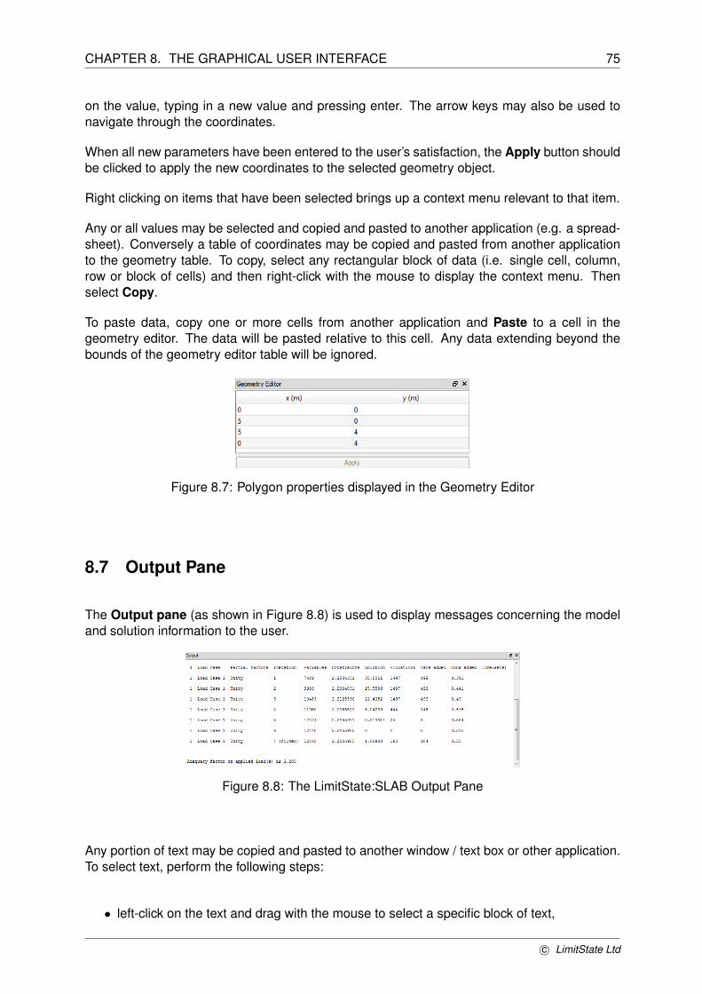


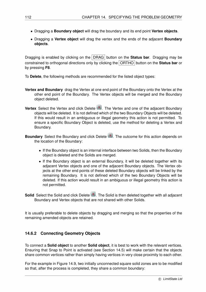


![Moodle Presentation [Version 2.0]](https://static.documents.pub/doc/80x56/559c40dd1a28abf3508b4650/moodle-presentation-version-20.jpg)


