Zonation, the clustering of organisms into distinct horizon-tal belts, is a common phenomenon of intertidal habitatsworldwide (Stephenson and Stephenson 1972, Ricketts et al.1985). The position of the upper and lower edges of these inter-tidal zones have long intrigued ecologists (Connell 1961, Paine1966, Stephenson and Stephenson 1972), and intertidal zonesare frequently used in ecological studies as indicators of com-parable environmental conditions across locations or over time(e.g., Johannesson et al. 1995, Gilman 2005). Zonation is thought
to reflect changes in patterns of emersion and immersion withvertical position on the shore. The timing and duration ofemersion modulate the degrees of desiccation, temperature,and salinity stress an organism experiences (Wolcott 1973,Stillman and Somero 1996, Wethey 2002, Dahlhoff 2004);conversely, the duration of immersion regulates feeding time,photosynthesis, and in some cases susceptibility to predation(Connell 1961, Paine 1966, Bell 1993). Thus zonation isthought to reflect species-specific physiological and ecologicaltolerance of immersion and emersion patterns. Many schemeshave been proposed over the years to associate intertidal zona-tion patterns in particular locations with fixed tidal elevationsor tidal regime statistics (Doty 1946, Ricketts et al. 1985). Yetattempts to generalize such local zonation schemes to largerregions are frequently unsuccessful (Stephenson and Stephen-son 1972). There is often great disparity in zonation patternsamong locations or within a location over time (Lawson 1957,Paine 1966, Leigh et al. 1987, Foster 1990).
Wave action alters patterns of zonation (Evans 1947, Lewis1964, Stephenson and Stephenson 1972, Lindegarth and Gam-
Evaluation of effective shore level as a method of characterizingintertidal wave exposure regimesSarah E. Gilman,1,2 Christopher D.G. Harley,3 Denise C. Strickland,1 Olivier Vanderstraeten,1 Michael J. O’Donnell,4,5
and Brian Helmuth1
1University of South Carolina, Department of Biological Sciences, Columbia, SC, USA2Present Address: Friday Harbor Laboratories, University of Washington, 620 University Road, Friday Harbor, WA, USA3University of British Columbia, Department of Zoology, Vancouver, BC, Canada4Stanford University, Hopkins Marine Station, Pacific Grove, CA, USA5Marine Science Institute, University of California, Santa Barbara, CA, USA
AbstractWave splash modifies the duration and timing of aerial exposure of intertidal organisms, influencing patterns of
vertical zonation, thermal stress, and the consequences of climate change. Harley and Helmuth (Limnol. Oceanogr.48:1498-1508, 2003) described a method for measuring effective shore level (ESL), a metric that combines the influ-ence of wave splash and tidal regime on patterns of emersion and immersion. They identified immersion events assharp drops in temperature recorded by submersible dataloggers and compared the tide height at the time of thetemperature drop to the wave height recorded by an offshore buoy. Here we explore the generality of this methodat 10 sites along the Pacific coast of North America spanning 14° of latitude. We deployed miniature temperatureloggers at fixed intertidal heights at each site and recorded temperatures at intervals of 5 to 15 min for periods ofup to 5 years. We use these data to explore the effects of different approaches to calculating temperature drops andwave heights, as well as variation in the buoy location, on ESL calculations. We present a software program(SiteParser) that can be used to identify temperature drops in a datalogger time series and also calculate daily andmonthly summary statistics of temperature. We show that ESL parameters provide a useful metric for comparingthe effects of wave action on immersion patterns within sites. We also introduce a metric of average wave run-upthat can be used to compare the effect of wave action on immersion patterns among more distant locations.
AcknowledgmentsThis study was funded by NSF award OCE-0323364 and NASA
NNG04GE43G to B.H. and by OCE-9985946 to Dr. Mark Denny, StanfordUniversity. Access to Tatoosh Island was kindly provided by the MakahTribal Nation and the United States Coast Guard. The Partnership forInterdisciplinary Studies of Coastal Oceans (PISCO) provided logisticalsupport at several field sites, and we are grateful to the many techniciansand students who assisted in the collection of field data.
feldt 2005). In some cases, lack of tolerance to high wave forcesmay limit local species composition in wave-exposed areas(Menge and Sutherland 1976). Waves may also increase theheight of water on the shore, effectively decreasing the fre-quency and duration of emersion and concomitant thermal anddesiccation stresses (Stephenson and Stephenson 1972, Rickettset al. 1985). Specifically, high wave action will cause a point onthe shore to behave as if it is effectively lower than its actual still-water tide height (Figure 1a). By comparing the observed timingof immersion for a point at a known tide height to its predictedimmersion pattern, based on a tide table, it is possible to esti-mate the point’s effective shore level. Such calculations havebeen made only occasionally (e.g., Glynn 1965, Druehl andGreen 1970), presumably because they are tedious and difficultto conduct comparatively for multiple locations.
Harley and Helmuth (2003) described a method for identi-fying immersion events from time series of intertidal temper-ature. Their method relied on miniature submersible tempera-ture dataloggers that store high-frequency (twice an hour orfaster) time series of temperature data for periods of 1 to 6months. Harley and Helmuth (2003) used a sudden sharp dropin temperature (3°C over 20 min) on a rising tide to identifyimmersion events during the daytime, when cooler seawaterengulfs a temperature logger that has previously been warm-ing from exposure to terrestrial climate. Once the tide heightand wave height at the time of the immersion event are iden-tified for many such events, regression can be used to calcu-late the effect of wave action on the tidal height of immersion(Figure 1b). The effective shore level (ESL) of a given point inthe intertidal zone is equal to the absolute shore level (ASL),the vertical distance above still-water chart datum, with equiv-alent emersion characteristics (timing and duration) in theabsence of waves (Figure 1a; see also Harley and Helmuth2003). This method should apply similarly to regions with lit-tle or no tidal fluctuation, although we have not tested it inthese situations.
The mean of all observed ESLs for a location describes theaverage tide height at which the location will transition fromemersed to immersed. The difference between the location’smean ESL and its ASL can be used as a measure of its averagewave run-up (AWR), literally an estimate of how far the location’seffective shore level is depressed by wave action (Figure 1b). AWRdepends on both wave height and local shoreline topographyand is a very different measure of wave exposure than wave force.Although both wave splash and wave force should increase withincreasing wave height, they need not be strongly correlated.For example, a site with a gently sloping shoreline may experi-ence a fairly low AWR because of the large distance that thewaves need to travel in the horizontal plane before moving veryfar in the vertical direction. In contrast, a steeply-sloped site mayexperience high AWR at even fairly low wave heights becauseall points on the shore are never far from the still-water tideline. Thus spatial patterns of AWR (and ESL), may not be cor-related with patterns of wave force.
In their introduction of the ESL technique, Harley andHelmuth (2003) conducted only a modest examination of therobustness of the ESL metric to changes in the temperaturethreshold used to identify drops. Here we examine more fullythe uses and limitations of the ESL approach. We first presenta software program (SiteParser) that automates the process ofidentifying temperature drops of a user-specified threshold.The program also calculates daily and monthly temperaturesummary statistics. We use data sets of rapid temperaturedrops generated by SiteParser to explore the ESL methodologyin more detail. Specifically, we compare the effect of changesin the magnitude of temperature drop threshold, in the mea-surement of wave height, and in the source of wave data onthe number and reliability of calculated temperature dropsand on the robustness of the wave height—immersion rela-
Gilman et al. Quantifying intertidal wave run-up
449
Fig. 1. (a) Schematic showing the effect of wave action on ESL. On acalm day, a point on the shore (circle) would not be immersed until thestill tide height exceeded its absolute shore level (ASL). The run-up ofwaves onshore lifts the effective water level, causing immersion at a lowertide height, and depressing the point’s effective shore level (ESL).(b) Sample ESL regression illustrating terminology used in this paper. Inthe main plot, the observed tidal height at the time of each temperaturedrop (ESL) is plotted against the significant wave height (h), and a linearregression is calculated. The left and lower plots show the frequency dis-tribution of ESL and h, respectively. The ASL is calculated by surveying thelocation relative to a known benchmark or estimated from the interceptof the ESL regression line (β0). The average wave run-up (AWR) is calcu-lated as the difference between ASL and the mean observed ESL, orbetween β0 and the ESL predicted from the regression equation for anaverage-sized wave. In this example, ASL and β0 differ by less than 5 cm,but larger differences are more common (e.g., Figure 4).
tionship. We introduce a modification to the calculation ofAWR for locations where ASL is not available. Finally, we applythe technique to quantitatively describe the wave splashregimes of multiple sites along the Pacific coast of the conti-nental United States. We show that ESL is a useful techniquefor comparing the effect of waves on immersion patternswithin a site, and that AWR can be used to make comparisonsamong more distant locations.
Materials and proceduresMaterials—Three time series are necessary to calculate a
wave height–immersion relationship: a temperature time seriesfor the specific location of interest, an observed or predictedtide height time series, and a concomitant time series of sig-nificant wave height. The temperature and tidal height timeseries must be of fairly high temporal resolution (< 30 minbetween samples); the temporal resolution of the wave heightdata set should be at least every 6 hours. Temperature timeseries may be collected using miniature, submersible tempera-ture dataloggers with a reasonably fast (< 5 min) thermal equi-libration time, such as TidbiTs (Onset Computer, Pocahassett,MA, USA) or iButtons (Maxim Integrated Products, Sunnyvale,CA, USA). Fitzhenry et al. (2004) and Helmuth (2002) discusssuch loggers in the context of intertidal thermal physiologicalstudies. Computer programs such as Tides and Currents(Nobeltec, Portland, OR, USA) or Xtide (www.flaterco.com)can be used to generate detailed tidal predictions for locationsworldwide. The U.S. National Ocean Service’s Center for Oper-ational Oceanographic Products and Services (NOS, tidesand-currents.noaa.gov) also collects tidal observations and con-structs predictions for many coastal locations in the UnitedStates. The U.S. National Data Buoy Center (NDBC, www.ndbc.noaa.gov) reports wave data from many U.S. and internationallocations. In this article, we also use wave height data frombuoys maintained by the Scripps Institution of Oceanography’sCoastal Data Information Program (CDIP, cdip.ucsd.edu).
SiteParser—Temperature drop events may be calculated byany of a number of mathematical or spreadsheet computerprograms (e.g., Excel, Matlab, SAS). Calculations require oneor more temperature time series for locations of interest and apredicted or observed time series of still-water tide height. Adrop is identified as a decrease in temperature greater than orequal to a specified threshold, within a fixed time interval(usually 20 min), and during an incoming tide (Harley andHelmuth 2003).
To facilitate such drop calculations, we developed theSiteParser program (Appendix 1), a stand-alone applicationthat runs on Windows systems. SiteParser requires a text fileas input, each line of which consists of the date and time,the predicted or observed tidal height, and the observedtemperature of one or more loggers. An unlimited numberof temperature time series may be included in the sameinput file. Once the user specifies the minimum magnitudeof temperature drop to count, the program will output as
separate files the time and tide height of all such tempera-ture drops observed on an incoming tide. In addition toidentifying temperature drops, SiteParser also automaticallycalculates daily and monthly temperature averages, maxima,minima, 97.9th percentile and 2.08th percentile (the maxi-mum and minimum temperature that loggers are exposed tofor at least half an hour; Fitzhenry et al. 2004), and per-centile ranges. SiteParser will also calculate average tempera-ture when the still-water tide height is above a user-specifiedlevel; this can be used to estimate water temperature duringperiods of logger immersion.
ESL regression calculation—The ESL regression equation iscalculated by regressing the tide height at the time of the tem-perature drop onto a measure of significant wave height forthe same time interval. The wave metric is usually the maxi-mum significant wave height observed over a period of 1 to 24 hpreceding the temperature drop event. Longer time windowsare necessary when wave data are collected from a distantbuoy because there may be a time lag before the wave heightrecorded by the offshore buoy reaches the temperature loggeronshore. We discuss more fully in the assessment section theeffect of buoy distance and wave time interval on the ESLregression function.
Standard least-squares linear regression is used to calcu-late the relationship between wave height and the tide at thetime of the drop. Any number of statistical software packages(e.g., SAS, JMP, R, Statview, but not Microsoft Excel, cfMcCullough and Wilson 2002) can be used to calculate theregression function. The regression equation is of the form:ESL = β0 + β1h, where ESL is the tide height at immersionand h is a measure of significant wave height preceding theimmersion. The slope of this equation (β1) usually has unitsof centimeters of tidal height per meter of wave height andrepresents the reduction effective in tidal height to the log-ger location of a 1-m increase in wave height. In other words,it estimates the number of centimeters below a point’s ASLthat the threshold for submergence will occur for each 1-mincrease in wave height. The intercept (β0) could be inter-preted as an estimate of the absolute shore level (ASL); wetest this assumption below. Harley and Helmuth (2003) useda log transformation of both dependent and independentvariables prior to regression; however, we have not found thatsuch a transformation improves either the regression fit or thenormality of errors.
Harley and Helmuth (2003) define the average wave run-upas the difference between a location’s ASL and the meanobserved ESL. We suggest a slight modification: replacing themean ESL with the predicted ESL from the regression equationevaluated at the mean wave height of the buoy. AWR can beused to compare the relative effect of wave action among dif-ferent locations within a site or among different sites. Wherethe ASL of a location is unknown, it can be estimated by β0
(see discussion below). We refer to both calculations inter-changeably as average wave run-up (AWR).
Data collection—All assessments were conducted from multi-year intertidal temperature time series collected from 10 sitesalong the Pacific Coast of the United States (Table 1) as part ofa long-term study of intertidal mussel temperatures (Helmuthand Hofmann 2001, Helmuth et al. 2002, Fitzhenry et al.2004). Each instrument recorded average temperatures at 10- to 15-min intervals. Three to seven instruments weredeployed at each site. Most instruments were placed at theapproximate vertical center (mid) of the mussel bed at eachsite. At some sites, instruments were placed in up to four addi-tional positions within the mussel bed: the upper (upper) orlower (low) edge of the bed, or halfway between the centerand either the upper limit (midupper) or lower limit (midlow).
For most sites, we used tidal prediction time series gener-ated at 10-min intervals from the Xtide Program. For someanalyses at Monterey, California, we used observed tidalheights reported by the NOS tide station in Monterey Bay(NOS9413450). Offshore wave height data were obtainedfrom the nearest NDBC or CDIP buoys (Table 1). At Mon-terey, nearshore wave data were also collected from aSeabird pressure transducer (Sea-Bird 26-03 Seagauge)located approximately 125 m offshore of the site (Helmuthand Denny 2003).
Accuracy testing of the SiteParser program—We compared the sta-tistics calculated by SiteParser for data from two sites in southernCalifornia (Alegria and Jalama, 34.47°N,120.28°W and 34.50°N,120.50°W) to calculations done by hand for each site using theMicrosoft Excel spreadsheet program. These summaries were inagreement. Additional testing was performed on other rockyintertidal data sets and from other types of environments,including salt marsh and shallow coral reef habitats (B. Helmuth,K. Schneider, J. Jost, and K. Castillo, unpublished data).
Effect of temperature threshold on the number and accuracy ofdrops—Fluctuations in terrestrial climate, such as sunset,clouds, or fog, may also produce sudden drops in temperaturewhen loggers are exposed at low tide. Such fluctuations maybe excluded by increasing the magnitude of the temperaturedrop threshold; however, increasing the drop magnitude mayalso exclude valid immersion events and reduce the totalnumber of events available for regression. Figure 2 shows thetotal number of drops and reliability, over 1 year, at multiple
Gilman et al. Quantifying intertidal wave run-up
451
Table 1. Study sites and summary of ESL regression results.
Alegria, CA 34.50 N,120.50 W cdip107 46.45 3 9 5 0.193–0.367 19–59 27.588–36.686
Lompoc, CA 34.72 N,120.61 W cdip076 58.85 4 12 4 0.033–0.221 24–164 16.588–58.193
Piedras, CA 35.67 N,121.29 W ndbc46028 54.69 4 3 5 0.350–0.410 37–60 62.534–81.843
Monterey, CA 36.62 N,121.90 W ndbc46042 48.54 4 6 5 0.300–0.424 12–171 53.056–94.332
(exposed)
Monterey, CA 36.62 N,121.90 W ndbc46042 48.54 2 6 6 0.377–0.582 199–229 28.408–44.260
(protected)
Strawberry Hill, 44.25 N,124.12 W ndbc46050 52.46 5 3 5 0.124–0.547 32–97 22.739–47.394
OR (exposed)
Strawberry Hill, 44.25 N,124.12 W ndbc46050 52.46 5 3 5 0.070–0.226 83–378 24.206–27.497
OR (protected)
Boiler Bay, OR 44.83 N,124.05 W ndbc46050 44.51 7 1 6 0.226–0.434 89–209 28.493–66.100
Colin’s Cove, WA 48.55 N,123.00 W ndbc46088 27.47 3 12 7 0.023–0.054 19–27 3.201–6.156
Tatoosh, WA 48.39 N,124.74 W ndbc46041 116.68 6 1 6 0.056–0.503 27–78 10.069–67.924
Fig. 2. (a-c) Drop reliability (proportion of temperature drops not coin-cident with a temperature drop in a terrestrial datalogger). (d-f) Totalnumber of drops identified over a year for a range of temperature dropthresholds at three sites. See Table 1 for site information. Loggers wereplaced at one of five vertical positions within mussel beds, ordered fromhighest to lowest as upper, midupper, mid, midlow, low. Logger locationsused in more than one figure retain the same symbol throughout.
datalogger locations at three of the sites listed in Table 1. Mon-terey is the only site with data for all five vertical positionswithin the mussel bed. To assess reliability we used a “terres-trial” datalogger, placed well above the highest tide line ateach location. An observed temperature drop at an intertidallogger was considered to be false if it occurred within 30 minof an observed drop at the terrestrial logger. This provides anestimate of the frequency of false temperature drops in thedata set, but may not identify all such drops.
The three sites show slight differences in the fraction ofdrops considered reliable (i.e., not coincident with an event inthe terrestrial logger) as a function of temperature threshold(Figure 2a-c), presumably reflecting local differences in thetemporal dynamics of terrestrial climate. Greater temperaturethresholds generally increased reliability and decreased thetotal number of drops. Low and midlow vertical positions alsoshowed greater reliability and fewer drops than higher loca-tions (Figure 2). Loggers at lower-shore positions spend lesstime overall exposed to air and experience lower maximumtemperatures, which reduces the likelihood of experiencing
spurious temperature drops relative to loggers higher in theintertidal zone. At all sites, temperature thresholds of around4° to 5°C were usually associated with ≥ 90% reliability and ≥ 100drops/year for mid and upper sites. Because of the overallfewer number of drops and higher reliability, a lower temper-ature threshold may be preferred for lower intertidal locations.
Effect of temperature threshold on the estimation of ESL parameters—Increasing the temperature threshold generally increases theR2 value of the ESL regression (Figure 3a-c), with one clearexception. At lower intertidal positions, particularly at Alegria,CA (Figure 3a), and Boiler Bay, OR (Figure 3b), R2 decreases atthe highest threshold levels. This presumably reflects a loss ofinformation from the exclusion of reliable data points by thehigh temperature threshold. Except for the lower intertidalloggers, the ESL slopes estimated for Alegria, CA (Figure 3d),and Boiler Bay, OR (Figure 3e), were relatively insensitive tochanges in the temperature threshold, with variation of lessthan 10 cm height/m wave common. Standard errors of theslope estimates were relatively small (< 10 cm) at the two sites(Figure 3g-h). In contrast, all logger locations at Monterey(Figure 3f) showed consistent declines in slope, even when R2
values were relatively constant. The standard errors of theMonterey slopes (Figure 3i) were also higher than at the othertwo sites. We cannot explain these observations.
The intercept of the ESL regression equation (β0) predictsthe effective shore level under a wave height of zero, and maybe useful as an estimate of a location’s surveyed, or absolute,tidal height (ASL). To test this hypothesis, we compared esti-mates of β0 to ASL values for 10 logger locations within theMonterey site. Surveyed tidal heights were measured with anAshtech Z-extreme GPS system (Thales Navigation, SantaClara, CA, USA). The difference between ASL and β0 rangedfrom less than 5 cm in the best case to more than 50 cm in theworst (Figure 4a). β0 tended to underestimate the actual ASL ofthe logger locations at Monterey, but improved at higher dropthresholds. The difference was generally greatest for highintertidal locations and probably reflects the lower reliabilityof drops (Figure 2a-c) at these locations. Standard errors of β0
were generally less than 25 cm (Figure 4b). This seems high,but may reflect idiosyncrasies of the Monterey site that arealso apparent in the high standard errors of β1 (Figure 3i).Unfortunately, ASL values were not available for any of theother study sites. Heights estimated by β0 were positively cor-related with observed ASL (r = 0.6972–0.9004, P < 0.05 for allthresholds), suggesting that β0 may be a useful measure of rel-ative tidal height even where it underestimates ASL. Morestringent drop threshold may improve the accuracy of β0 as anestimate of ASL, but will require a longer temperature timeseries to generate enough data points.
Effect of wave time interval—Generally, the more distant anoffshore buoy is from the intertidal shore, the longer time itwill take for a wave recorded at the buoy to reach the shoreand the greater the difference in wave environments betweenthe two. Increasing the time window over which the wave
Gilman et al. Quantifying intertidal wave run-up
452
Fig. 3. (a-c) R 2; (d-f) slope; and (g-i) standard error of the slope calcu-lated for the same range of drop thresholds and sites examined in Figure 2.Regressions for Alegria and Boiler Bay used a 1-h wave window; for Mon-terey, a 6-h window. Any regression with less than 10 data points wasexcluded. Data for Alegria and Boiler Bay are from a slightly different timeinterval than those presented in Figure 2, but all regressions used a singleyear of data. Logger locations used in more than one figure retain thesame symbol throughout.
metric is calculated may mitigate at least the first of these twoproblems. Harley and Helmuth (2003) only used the maxi-mum wave for the calendar day. We compared the maximumwave calculated for windows of 1, 3, 6, 12, and 24 h before theobserved temperature drop for seven logger locations at theBoiler Bay site (Figure 5). The R2 of the ESL regression showedonly moderate variation in response to the wave time window,but there was a clear decline in R2 at the longest time window(24 h). Slopes also tended to flatten at longer time windows.This probably reflects the overall decline in the regression fit,as maximum wave heights at the buoy become a progressivelypoorer metric of onshore wave action at the time of a temper-ature drop at the longer time intervals. Longer time intervalsshould be associated with larger maximum waves, because ofthe larger number of wave heights sampled, and this may alsoexplain some of the slope change. Average wave run-up tendedto decrease slightly at higher time windows, but run-up wasgenerally less sensitive to time window than slope. Overallthere was little effect of the time window on ESL parameters,particularly in comparison to the effect of changing the drop
Gilman et al. Quantifying intertidal wave run-up
453
Fig. 4. (a) Difference between the predicted ESL intercept and measuredASL as a function of temperature drop threshold for 10 logger locations atMonterey. (b) Standard error of the ESL intercept. All regressions weredone using wave data from NDBC46042 with a 6-h time window. Symbolsthat match those used in Figures 1 and 2 indicate the same logger loca-tions. ASL values (in cm): upper1 = 195.1, mid3 = 185.02, mid2 = 181.24,mid4 = 172.83, midupper1 = 171.05, mid1 = 162.10, mid5 = 138.98,mid6 = 130.33, midlow1 = 110.98, low1 = 71.02.
Fig. 5. (a) R2; (b) average wave run-up; (c) slope; and (d) standard errorof the slope calculated for ESL regressions under varying time windows ofwave data for logger locations at Boiler Bay. A 4°C temperature drop wasused in all calculations.
threshold (Figure 5 vs. Figure 3). Because both ESL parametersand the run-up statistic appear robust to changes in the wavemetric, we recommend using the wave-time interval that max-imizes the R2 of the ESL regression.
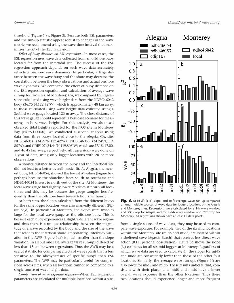
Effect of buoy distance on ESL regression—In most cases, theESL regression uses wave data collected from an offshore buoylocated far from the intertidal site. The success of the ESLregression approach depends on such wave data accuratelyreflecting onshore wave dynamics. In particular, a large dis-tance between the wave buoy and the shore may decrease thecorrelation between the buoy observations and actual onshorewave dynamics. We compared the effect of buoy distance onthe ESL regression equation and calculation of average waverun-up for two sites. At Monterey, CA, we compared ESL regres-sions calculated using wave height data from the NDBC46042buoy (36.75°N,122.42°W), which is approximately 48 km away,to those calculated using wave height data collected using aSeabird wave gauge located 125 m away. The close distance ofthis wave gauge should represent a best-case scenario for meas-uring onshore wave height. For this analysis, we also usedobserved tidal heights reported for the NOS site in MontereyBay (NOS9413450). We conducted a second analysis usingdata from three buoys located close to the Alegria, CA, site:NDBC46054 (34.27°N,122.42°W), NDBC46053 (34.24°N,119.85°W), and CDIP107 (34.44°N,119.803°W) which are 27.15, 47.00,and 46.45 km away, respectively. All regressions were done on1 year of data, using only logger locations with 20 or moreobservations.
A shorter distance between the buoy and the intertidal sitedid not lead to a better overall model fit. At Alegria, the near-est buoy, NDBC46054, showed the lowest R2 values (Figure 6a),perhaps because the shoreline faces south to southeast andNDBC46054 is west to northwest of the site. At Monterey, thelocal wave gauge had slightly lower R2 values at nearly all loca-tions, and this may be because the gauge samples less fre-quently than the offshore buoy (every 6 hours vs. hourly).
At both sites, the slopes calculated from the different buoysfor the same logger location were also markedly different (Fig-ure 6c,d). In particular at Monterey, the slopes were twice aslarge for the local wave gauge as the offshore buoy. This isbecause each buoy experiences a slightly different wave regimeand thus there is a unique relationship between the magni-tude of a wave recorded by the buoy and the size of the wavethat reaches the intertidal shore. Importantly, interbuoy vari-ation in the AWR (Figure 6e,f) is much smaller than the slopevariation. In all but one case, average wave run-ups differed byless than 15 cm between regressions. Thus the AWR may be auseful statistic for comparing effects of wave splash that is lesssensitive to the idiosyncrasies of specific buoys than ESLparameters. The AWR may be particularly useful for compar-isons across sites, when all locations cannot be compared to asingle source of wave height data.
Comparison of wave exposure regimes—When ESL regressionparameters are calculated for multiple locations within a site,
from a single source of wave data, they may be used to com-pare wave exposure. For example, two of the six mid locationswithin the Monterey site (mid5 and mid6) are located withina sheltered cove (Agassiz Beach) that receives less direct waveaction (B.H., personal observation). Figure 6d shows the slope(β1) estimates for all six mid loggers at Monterey. Regardless ofwhich wave data are used to calculate β1, the slopes for mid5and mid6 are consistently lower than those of the other fourlocations. Similarly, the average wave run-ups (Figure 6f) arealso lower for mid5 and mid6. These results indicate that, con-sistent with their placement, mid5 and mid6 have a loweroverall wave exposure than the other locations. Thus thesetwo locations should experience longer and more frequent
Gilman et al. Quantifying intertidal wave run-up
454
Fig. 6. (a-b) R2; (c-d) slope; and (e-f) average wave run-up comparedamong multiple sources of wave data for loggers locations at the Alegriaand Monterey sites. Regressions were calculated for a 1-h wave windowand 5°C drop for Alegria and for a 6-h wave window and 5°C drop forMonterey. All regressions shown have at least 10 data points.
periods of aerial exposure than locations of equivalent ASLnear the other four loggers.
To compare overall patterns of wave exposure across thePacific coast of the United States, we calculated ESL regressionsand average wave run-ups for 10 sites using a range of dropthresholds (3° to 7°C per 20 min) and wave time lag intervals(from 1 to 24 h). ESL regressions were calculated separately forup to seven replicate logger locations within the center of themussel bed at each site, and the best overall combination ofwave time window and temperature drop threshold was cho-sen from the resulting R2 values (Table 1). The regression fit (R2)varied markedly among sites, and was particularly poor at themost wave-protected sites (Table 1). For example, R2 values atColin’s Cove, WA, were always below 0.1. This is likely bothbecause the site occurs in a highly wave-sheltered portion ofthe coast (inside the Strait of Juan de Fuca), and because thenearest available buoy is west of the island whereas Colin’sCove is on the eastern shore. A low R2 implies there is little rela-tionship between offshore wave and data and onshore immer-sion patterns, and should be expected for a wave-sheltered site.In contrast, at three sites (Monterey, CA; Strawberry Hill, OR;and Tatoosh, WA) R2 values exceeded 0.5.
Differences in AWR among sites (Figure 7) reflect knowndifferences in wave exposure, indicating that AWR is a reason-able method of quantifying large-scale variation in wave expo-sure. For example, two of the 10 sites, Alegria, CA, and Colin’sCove, WA, are highly wave sheltered, occurring within theSouthern California Bight and Strait of Juan de Fuca, respec-tively. As expected, these two sites showed the lowest overallAWR values, indicating that wave action has little effect on
immersion patterns. Similarly, when wave-exposed and wave-protected locations were identified a priori within both theMonterey, CA, and Strawberry Hill, OR, sites, the AWR valueswere generally lower at the wave-protected locations.
Average wave run-up varies considerably both among andwithin sites. Among the four California sites, there is a trendof increasing AWR with latitude. But no such trend is appar-ent in Oregon or Washington. This may be due in part to thespecific locations selected for logger deployment within eachsite. For instance, the Tatoosh Island loggers were deployed ina south-facing cove that was moderately protected from thepredominantly west to northwesterly swell (see map in Harleyand Helmuth 2003). Indeed, our calculations of AWR revealedsizeable variation in wave exposure within locations. Forexample, the range of AWR values exceeds 50 cm within theMonterey, CA, wave-exposed location, the Strawberry Hill,OR, wave-exposed location, and the Tatoosh Island, WA, loca-tion. This variation is not correlated with the length of shore-line sampled, which ranges from 25 to 500 m, depending onthe site. This suggests that wave exposure can be quite variablewithin sites, even among locations that appear superficiallyquite similar. Similarly, Denny et al. (2004) and Helmuth andDenny (2003) found greater than 5-fold variation in waveforces along a 300-m transect within the Monterey site.
Discussion and recommendations Understanding the processes that control the distribution and
abundance of species is a fundamental goal of ecology. Few pat-terns of distribution and abundance are as striking as the bandsof intertidal zonation common to shores worldwide (Evans 1947,Lawson 1957, Connell 1961, Lewis 1964, Paine 1966, Stephensonand Stephenson 1972, Leonard et al. 1999). Wave exposure,through both wave force and changes in immersion patterns, haslong been known to alter patterns of abundance and zonation(Stephenson and Stephenson 1972, Druehl and Green 1982,Ricketts et al. 1985, Denny and Paine 1998, Lindegarth andGamfeldt 2005), yet few studies have quantitatively describedspatial differences in wave action or the consequences for speciesdistributions (Lindegarth and Gamfeldt 2005). Our analysis of theESL regression method, originally presented by Harley andHelmuth (2003), demonstrates the usefulness of ESL regressionparameters for characterizing differences in both tidal height andwave splash among neighboring points along a shore. Our analy-ses also suggest that average wave run-up is a useful metric forcomparing wave exposure among more distant locations.
When ESL parameters for all locations can be calculatedfrom a single source of wave data, such as when all measuredpoints lie along a single shoreline, the parameters of the ESLregression equation can be used to estimate differences inboth wave exposure and absolute shore level. The ESL inter-cept (β0) may be used as an estimate of absolute shore level(ASL), although we found that β0 frequently underestimatedthe true ASL. We recommend that β0 be considered primarilya relative index of ASL, suitable for comparisons within loca-
Gilman et al. Quantifying intertidal wave run-up
455
Fig. 7. Average wave run-up (AWR) for the center of the mussel bed at11 sites along the U.S. Pacific coast. AWR was calculated for all availablemid temperature loggers, for the combination of temperature thresholdand wave time window that maximized R2 values within each site (Table 1).The total length of shoreline sampled at each site ranged from 25 to 500 m.Sites are arranged from south to north along the x-axis; exact latitude andlongitude are listed in Table 1.
tions. The slope of the ESL regression (β1) is an estimate of thedecrease in effective shore level as wave height increases. Itmay be used for direct comparison of wave splash among loca-tions. Greater values of β1 indicate greater relative wave splashand a reduction in the frequency and duration of immersion.However, because the magnitude of β1 depends on the rela-tionship between onshore and offshore wave heights, valuesof β1 have no literal meaning outside a single study area.
All calculations for within-location comparisons must alsobe done using identical temperature thresholds, tidal data,and wave height metrics. Care must be taken in choosing atemperature threshold that will exclude false temperaturedrops during aerial exposure, while minimizing the loss ofvalid data. False drops occur during low tide under suddenchanges in terrestrial climate such as fog, rain, or sunset. Theyare most common at locations with long aerial exposures,mainly high intertidal or highly wave-protected sites. Becausethe mussel beds used for analyses in this article occur rela-tively high in the intertidal zone (approximately the top quar-tile of tidal range at most locations) our sites should have alarge frequency of false drops relative to other parts of theintertidal zone and thus present a conservative test of the ESLapproach. At lower intertidal locations, we found that hightemperature drop thresholds may decrease R2 by excludingvalid data points. Thus we recommend screening a large rangeof temperature drop thresholds and wave time windows tofind one that maximizes R2 values across all sites of interest.Appendix 2 contains sample SAS code for conducting suchscreenings; other statistical programs can also be used.
Because ESL regression parameters are highly sensitive tothe choice of wave height data, they are not directly compa-rable among locations that differ in their source of waveheight measurements. Instead, we propose the average waverun-up (AWR) as a metric for comparing wave exposure amongdistant locations. The AWR is the average change in tidalheight of immersion due to wave action. If a site’s ASL isknown or can be measured against a surveyed benchmark, theAWR can be calculated as the difference between ASL and themean tide height of observed temperature drops. When ASL isunknown, AWR may be calculated from the ESL regression asthe mean wave height multiplied by the absolute value of β1.Our analyses suggest that AWR calculated in this way is rela-tively robust to variation in the source of wave height data. Inparticular, we found that estimates of AWR calculated fromdifferent sources of wave data usually differed by less than 15cm, and we suggest a threshold of 25 to 30 cm be used beforeconsidering two AWR values to be different. Comparison ofAWR values among 11 sites spanning ~1400 km demonstratedthat AWR successfully predicted relative rankings of waveexposure based on a priori knowledge of wave action orcoastal morphology.
Overall our analyses suggest that effective shore levelregression is a useful and robust method for local estimates oftidal height and wave exposure regime and for calculating
average wave run-ups, which may be used to compare waveexposures at larger spatial scales. A number of other tech-niques exist for quantifying wave exposure as discrete or con-tinuous values. Categorical definitions based on a location’sbiological or physical properties are frequently used in thepublished literature, but may be subject to idiosyncrasies ofthe researcher (Lindegarth and Gamfeldt 2005). One commonquantitative approach is based on the measurement of disso-lution of plaster, but its interpretation is complicated by dif-ferences in temperature and other conditions among sites(Muus 1968, Doty 1971, Porter et al. 2000). A number of tech-niques for quantifying maximum wave force exist (Denny 1985,Bell and Denny 1994); however, the relationship betweenwave force and changes to immersion/emersion patterns isunknown. Local wave height can be measured directly by sen-sors (e.g., Helmuth and Denny 2003), but such sensors may becostly. A number of schemes also exist to estimate local waveheight from coastal morphology and wind data (Ruuskanen etal. 1999, Lindegarth and Gamfeldt 2005). The ESL regressionmethod relies on relatively low-cost temperature dataloggersthat may already be in place for other reasons. Our analysessuggest that ESL and AWR provide an accurate, quantitativemeasurement of the thermal aspects of wave exposure thatcan be compared both locally and among geographically dis-tant sites. Such measurements should prove useful to intertidalecology for studies of the effects of wave splash on speciesinteractions, intraspecific variation in growth and morphol-ogy, patterns of intertidal zonation, and spatial variation inthermal stress.
ReferencesBell, E. C. 1993. Photosynthetic response to temperature and
desiccation of the intertidal alga Mastocarpus papillatus.Mar. Biol. 117:337-346.
——— and M. W. Denny. 1994. Quantifying “wave exposure”:a simple device for recording maximum velocity and resultsof its use at several field sites. J. Exp. Mar. Biol. Ecol. 181:9-29.
Connell, J. H. 1961. The influence of interspecific competitionand other factors on the distribution of the barnacleChthamalus stellatus. Ecology 42:710-723.
Dahlhoff, E. P. 2004. Biochemical indicators of stress andmetabolism: applications for marine ecological studies. Annu.Rev. Physiol. 66:183-207.
Denny, M. W. 1985. Water motion. In M. M. Littler, D. S. Litter[eds.] Ecological Field Methods: Macroalgae. Handbook of Phy-cological Methods. New York, Cambridge Univ. Press, p. 7-32.
———, B. Helmuth, G. H. Leonard, C. D. G. Harley, L. J. Hunt,and E. K. Nelson. 2004. Quantifying scale in ecology: les-sons from a wave-swept shore. Ecol. Monogr. 74:513-522.
——— and R. T. Paine. 1998. Celestial mechanics, sea-levelchanges, and intertidal ecology. Biol. Bull. 194:108-115.
Doty, M. S. 1946. Critical tide factors that are correlated withthe vertical distribution of marine algae and other organ-isms along the Pacific Coast. Ecology 27:315-328.
———. 1971. Measurement of water movement in reference tobenthic algal growth. Botanica marina 14:32-35.
Druehl, L. D., and J. M. Green. 1970. A submersion-emersionsensor, for intertidal biological studies. J. Fish. Res. Board Can.27:401.
———. 1982. Vertical distribution of intertidal seaweeds asrelated to patterns of submersion and emersion. Mar. Ecol.Prog. Ser. 9:163-170.
Evans, R. G. 1947. The intertidal ecology of selected localitiesin the Plymouth neighbourhood. J. Mar. Biol. Assoc. U.K.27:173-218.
Fitzhenry, T., P. M. Halpin, and B. Helmuth. 2004. Testing theeffects of wave exposure, site, and behavior on intertidalmussel body temperatures: applications and limits of tem-perature logger design. Mar. Biol. 145:339-349.
Foster, M. S. 1990. Organization of macroalgal assemblages inthe northeast Pacific: the assumption of homogeneity andthe illusion of generality. Hydrobiologia 192:21-33.
Gilman, S. E. 2005. A test of Brown’s principle in the intertidallimpet Collisella scabra (Gould, 1846). J. Biogeogr. 32:1583-1589.
Glynn, P. W. 1965. Community composition, structure, and inter-relationships in the marine intertidal Endocladia muricata–Balanus glandula association in Monterey Bay, California.Beaufortia 12:1-98.
Harley, C. D. G., and B. S. T. Helmuth. 2003. Local andregional scale effects of wave exposure, thermal stress, andabsolute vs. effective shore level on patterns of intertidalzonation. Limnol. Oceanogr. 48:1498-1508.
Helmuth, B. 2002. How do we measure the environment?Linking intertidal thermal physiology and ecology throughbiophysics. Integr. Comp. Biol. 42:837-845.
——— and M. W. Denny. 2003. Predicting wave exposure inthe rocky intertidal zone: do bigger waves always lead tolarger forces? Limnol. Oceanogr. 48:1338-1345.
———, C. D. G. Harley, P. Halpin, M. O’Donnell, G. E. Hofmann, and C. Blanchette. 2002. Climate changeand latitudinal patterns of intertidal thermal stress. Science298:1015-1017.
——— and G. E. Hofmann. 2001. Microhabitats, thermal het-erogeneity, and patterns of physiological stress in the rockyintertidal zone. Biol. Bull. 201:374-384.
Johannesson, K., E. Rolan-Alvarez, and A. Ekendahl. 1995.Incipient reproductive isolation between two sympatricmorphs of the intertidal snail Littorina saxatilis. Evolution 49:1180-1190.
Lawson, G. W. 1957. Seasonal variation of intertidal zonationon the coast of Ghana in relation to tidal factors. J. Ecol. 45:831-860.
Leigh, E. G., R. T. Paine, J. F. Quinn, and T. H. Suchanek. 1987.Wave energy and intertidal productivity. Proc. Nat. Acad.Sci. U. S. A. 84:1314-1318.
Leonard, G. H., P. J. Ewanchuk, and M. D. Bertness. 1999. Howrecruitment, intraspecific interactions, and predation controlspecies borders in a tidal estuary. Oecologia 118:492-502.
Lewis, J. R. 1964. The Ecology of Rocky Shores. English Univ.Press, UK.
Lindegarth, M., and L. Gamfeldt. 2005. Comparing categoricaland continuous ecological analyses: effects of “wave expo-sure” on rocky shores. Ecology 86:1346-1357.
McCullough, B. D., and B. Wilson. 2002. On the accuracy ofstatistical procedures in Microsoft Excel 2000 and Excel XP.Comput. Stat. Data Anal. 40:713-721.
Menge, B. A., and J. P. Sutherland. 1976. Species diversity gra-dients synthesis of the roles of predation competition andtemporal heterogeneity. Am. Nat. 110:351-369.
Muus, B. J. 1968. A field method for measuring “exposure”by means of plaster balls: a preliminary account. Sarsia 34:61-68.
Paine, R. T. 1966. Food web complexity and species diversity.Am. Nat. 100:65-75.
Porter, E. T., L. P. Sanford, and S. E. Suttles. 2000. Gypsum dis-solution is not a universal integrator of water motion. Lim-nol. Oceanogr. 45:145-158.
Ricketts, E. F., J. Calvin, J. W. Hedgpeth, and D. W. Phillips.1985. Between Pacific Tides. Stanford, CA, Stanford Univer-sity Press.
Ruuskanen, A., S. Back, and T. Reitalu. 1999. A comparison oftwo cartographic exposure methods using Fucus vesiculo-sus as an indicator. Mar. Biol. 134:139-145.
Stephenson, T. A., and A. Stephenson. 1972. Life BetweenTidemarks on Rocky Shores. San Francisco, CA, W. H.Freeman.
Stillman, J. H., and G. N. Somero. 1996. Adaptation to tem-perature stress and aerial exposure in congeneric species inintertidal porcelain crabs (genus Petrolisthes): correlation ofphysiology, biochemistry and morphology with verticaldistribution. J. Exp. Biol. 199:1845-1855.
Wethey, D. S. 2002. Biogeography, competition, and microcli-mate: the barnacle Chthamalus fragilis in New England.Integr. Comp. Biol. 42:872-880.
Wolcott, T. G. 1973. Physiological ecology and intertidal zona-tion in limpets (Acmaea): a critical look at “limiting fac-tors.” Biol. Bull. 145:389-422.