ISSN 2042-2695

CEP Discussion Paper No 1075

September 2011

Rising Wage Inequality and Postgraduate Education

Joanne Lindley and Stephen Machin

Abstract This paper considers what has hitherto been a relatively neglected subject in the wage

inequality literature, albeit one that has been becoming more important over time, namely the

role played by increases in postgraduate education. We document increases in the number of

workers with a postgraduate qualification in the United States and Great Britain. We also

show their relative wages have risen over time as compared to all workers and more

specifically to graduates with only a college degree. Consideration of shifts in demand and

supply shows postgraduates and college only workers to be imperfect substitutes in

production and that there have been trend increases over time in the relative demand for

postgraduate vis-à-vis college only workers. These relative demand shifts are significantly

correlated with technical change as measured by changes in industry computer usage and

investment. Moreover, the skills sets possessed by postgraduates and the occupations in

which they are employed are significantly different to those of college only graduates. Over

the longer term period when computers have massively diffused into workplaces, it turns out

that the principal beneficiaries of this computer revolution has not been all graduates, but

those more skilled workers who have a postgraduate qualification. This has been an important

driver of rising wage inequality amongst graduates over time.

JEL Keywords: Wage inequality; postgraduate education; computers.

JEL Classifications: J24; J31

This paper was produced as part of the Centre’s Labour Markets Programme. The Centre for

Economic Performance is financed by the Economic and Social Research Council.

Acknowledgements We would like to thank Sarah Turner, our discussant at the 2011 CESifo

Economics of Education workshop, and participants in the 2011 CEP annual conference, the

IWAEE workshop and the WPEG conference for a number of helpful comments and

suggestions.

Joanne Lindley is a Senior Lecturer in Economics at the University of Surrey. Stephen

Machin is Research Director at the Centre for Economic Performance, London School of

Economics and Professor of Economics at University College London.

Published by

Centre for Economic Performance

London School of Economics and Political Science

Houghton Street

London WC2A 2AE

All rights reserved. No part of this publication may be reproduced, stored in a retrieval

system or transmitted in any form or by any means without the prior permission in writing of

the publisher nor be issued to the public or circulated in any form other than that in which it

is published.

Requests for permission to reproduce any article or part of the Working Paper should be sent

to the editor at the above address.

J. Lindley and S. Machin , submitted 2011

1

1. Introduction

Rising wage differentials between education groups have been identified as a key

feature of rising wage inequality in a number of countries (most notably the US and

UK, but also elsewhere).1 Rising relative wages for college educated workers, despite

their increased numbers, and the increased relative demand for workers that are more

educated (and the drivers of these increases) have featured prominently in discussions

of why overall wage inequality has risen.

One feature of the increased supply of college educated workers is that over

time more and more individuals have not stopped their education once graduating

with a first degree. Rather, they have gone on to acquire postgraduate qualifications.

In fact, in 2009 in both the countries we study in this paper (the United States and

Great Britain) just over 10 percent of the workforce (or just over 35 percent of all

college graduates) have a postgraduate qualification. It seems natural therefore to ask

whether this rise in postgraduate education has been connected to increased wage

inequality.

To our knowledge, this question has not yet received much attention from the

contributors to the rising wage inequality literature. Part of the reason may be that the

move to a significant share of the workforce possessing a postgraduate qualification is

a relatively recent phenomenon. Postgraduate education does feature as a focus of one

US paper (by Eckstein and Nagypal, 2004) which studies trends in overall wage

inequality in the US from 1961 to 2002 and, unlike others in the literature, does

highlight rising wage differentials for workers with postgraduate degrees. Also,

whilst not their main focus, there are also several references to rising postcollege

wages in the US in Autor, Katz and Kearney (2008) where they argue this feature of

1 See Acemoglu and Autor (2010) for an up to date review of this literature.

2

wage trends is difficult to rationalise in the standard two skill CES production

approach they favour.2

In terms of the potential importance of the issue, it is noteworthy that when

Lemieux (2006a) looks at all postsecondary education, rather than just college only

graduates, in a decomposition of inequality changes between the mid-1970s and mid-

2000s he concludes that ‘Understanding why postsecondary education, as opposed to

other observed or unobserved measures of skills, plays such a dominant role in

changes in wage inequality should be an important priority for future research'

[Lemieux, 2006a, p.199].

To date in the wage inequality research area, the main focus has been on the

temporal evolution of particular wage differentials and measures of education supply.

For example, the influential US papers of Katz and Murphy (1992), Card and

Lemieux (2001) and Autor, Katz and Kearney (2008) all consider the evolution

through time of one specific educational wage differential, the college only (i.e. 16

years of US education) to high school graduate wage gap (i.e. 12 years of education).

Similarly, in what has become known as the canonical supply-demand model of the

labour market (introduced by Katz and Murphy, 1992, but originating from

Tinbergen’s, 1974, model of the race between demand and supply) is modelled for

just two (aggregated) education groups: ‘college equivalent’ workers and ‘high school

equivalent’ workers.3

2 Acemoglu and Autor (2010) also present charts showing faster wage growth amongst the postgraduate group and the 'convexification' of the wage returns to education over time that has resulted from this. 3 In their estimation of relative supply-demand models in the US labour market, these authors make assumptions on the labour supply of the following five groups of workers: workers with a high school degree supply one ‘high school equivalent’, whilst workers with less than a high school degree supply a (relative wage weighted) proportion of this; workers with a college degree supply one ‘college equivalent’, whilst workers with a postgraduate degree supply a (relative wage weighted) mark up of this; and, finally, the intermediate group with some college are split between the two groups (Katz and

3

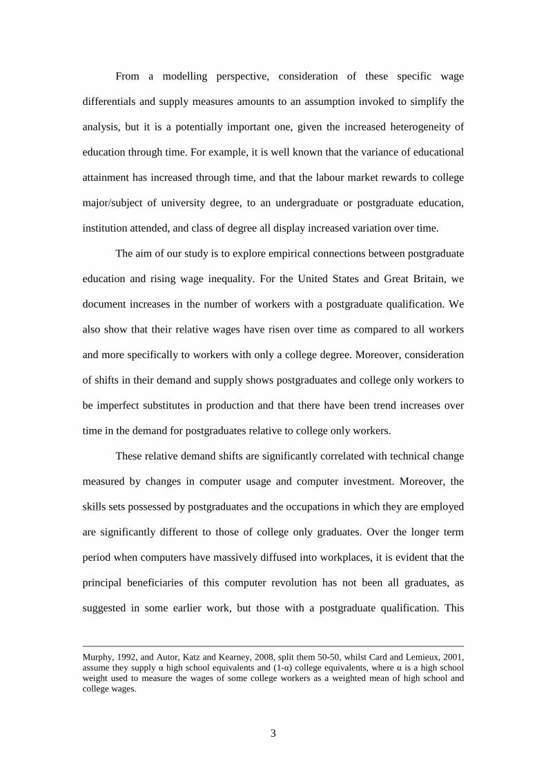
From a modelling perspective, consideration of these specific wage

differentials and supply measures amounts to an assumption invoked to simplify the

analysis, but it is a potentially important one, given the increased heterogeneity of

education through time. For example, it is well known that the variance of educational

attainment has increased through time, and that the labour market rewards to college

major/subject of university degree, to an undergraduate or postgraduate education,

institution attended, and class of degree all display increased variation over time.

The aim of our study is to explore empirical connections between postgraduate

education and rising wage inequality. For the United States and Great Britain, we

document increases in the number of workers with a postgraduate qualification. We

also show that their relative wages have risen over time as compared to all workers

and more specifically to workers with only a college degree. Moreover, consideration

of shifts in their demand and supply shows postgraduates and college only workers to

be imperfect substitutes in production and that there have been trend increases over

time in the demand for postgraduates relative to college only workers.

These relative demand shifts are significantly correlated with technical change

measured by changes in computer usage and computer investment. Moreover, the

skills sets possessed by postgraduates and the occupations in which they are employed

are significantly different to those of college only graduates. Over the longer term

period when computers have massively diffused into workplaces, it is evident that the

principal beneficiaries of this computer revolution has not been all graduates, as

suggested in some earlier work, but those with a postgraduate qualification. This

Murphy, 1992, and Autor, Katz and Kearney, 2008, split them 50-50, whilst Card and Lemieux, 2001, assume they supply α high school equivalents and (1-α) college equivalents, where α is a high school weight used to measure the wages of some college workers as a weighted mean of high school and college wages.

4

appears to have been a feature of the changing labour market as wage inequality has

risen in both the United States and Great Britain. This has been an important driver of

rising wage inequality amongst graduates over time.

The remainder of the paper is structured as follows. In Section 2, we document

changes in postgraduate education in the United States and Great Britain. We also

present initial descriptive evidence on changes in the relative wages of postgraduates

compared to other workers. In Section 3, we show results from estimating models of

the relative demand and supply of workers with different levels of education, placing

a specific focus on whether one can identify differential supply effects and trend shifts

for postgraduate workers. Section 4 considers the role that technology change,

especially the computer revolution, has played in explaining the observed shifts in

wage inequality and relative demand connected to the rise in postgraduate education.

We also consider differences in skills and job tasks of postgraduate and college only

workers. In Section 5, we address a relevant aspect of postgraduate heterogeneity

when, albeit for a shorter time period than we were able to use earlier in the paper, we

study whether there are notable differences for different postgraduate qualifications

(Master's degrees and doctorates). This includes analysis of wage and employment

trends, and study of differences in occupations of these groups of workers. Finally,

Section 6 concludes.

2. Changes in Postgraduate Employment and Wages

Rising Wage Inequality and Education

The broad motivation underpinning this paper comes from the observation that wage

inequality has risen rapidly in the United States and Great Britain over the last thirty

to forty years. To see this, consider Figure 1 that shows the 90-10 ratio of log (weekly

5

wages) for full-time workers (and in the case of the US, full year workers) from the

March Current Population Survey (CPS) for the United States and New Earnings

Survey/Annual Survey of Hours and Earnings (NES/ASHE) for Great Britain.4 The

Figure shows the evolution of the 90-10 ratio for men and women in the US between

1963 and 2009 and for GB between 1970 and 2009. In both countries, for both sexes,

overall wage inequality measured by the 90-10 stands at a substantially higher level in

the final year, and there is a strong trend upwards in both countries starting from

somewhere around mid 1960s in the US and the late 1970s in Britain.

As noted in the introduction, a focus in the literature on understanding rising

wage inequality has been to study between-group and within-group changes in

inequality. By far the most attention in the former category has been on studying wage

gaps between workers with different education levels, as rising wage gaps between

high and low education workers have been shown to be important determinants of

rises in overall wage inequality (see the reviews of Katz and Autor, 1999, and

Acemoglu and Autor, 2010, for more details).

In the existing work, however, the emphasis has to date almost always been

placed on studying the evolution through time of rather narrowly defined wage

differentials. In the US literature, the usual differential of focus is the college

only/high school graduate wage gap (i.e. the wage gap between workers with exactly

16 and 12 years of education). This fixed four year gap in schooling between college

only and high school graduates has the advantage that is should yield a good measure

of the college wage premium. However, it does select a specific group of graduates,

4 The March CPS is used for the US as it has a time series with wage and education data running as far back as 1963. The NES/ASHE data is used for GB as it has wage data back to 1970. However, it does not contain an education variable and so we cannot go as far back in our analysis that requires education data for GB - for this we use a combination of General Household Survey data (from 1977 to 1992) and the much larger sample sizes from the Labour Force Survey (from 1993 onwards when it first recorded earnings information).

6

eliminating those with more advanced postgraduate qualifications. Authors in this

literature are certainly aware of this and sometimes report additional estimates looking

at the wage gap between workers with 16 or more years of education (i.e. college only

and postgraduates, or college plus) as compared to workers with a high school degree.

In Card and Lemieux’s (2001) analysis, for example, they state that, based on data

running up to 1995, it makes little difference.

We believe there is good reason to revisit this question. First, wage inequality

has risen within the college plus group. Consider Figure 2, which shows the 90-10

ratio for all male and female graduates in the US and GB samples, again running from

1963 to 2009 in the US and now (because of requiring a consistent education variable)

from 1977 to 2009 in GB using the General Household Survey (1977 to 1992) and

Labour Force Survey (1993 to 2009). The Figure shows significant rises in graduate

wage inequality, a feature we investigate further in this paper to see if there are

differences between graduate workers with and without postgraduate qualifications.

Second, the relative employment and wages of postgraduate versus college only

workers has shifted through time. This is especially the case in the time periods after

the data used in existing work that does consider both college only and college plus

measures. We show this in the next sub-section.

Trends in Postgraduate Employment and Wages

Table 1 shows the employment shares of all graduates (college degree or

higher), postgraduates and college only employment shares and the postgraduate share

amongst graduates for the United States and Great Britain over time. The upper panel

of the Table shows that the overall graduate proportion is higher in the US, and has

risen from 0.14 in 1963 through to 0.36 by 2009. The decade by decade changes

reveal a well known pattern, where the employment share of graduates rose rapidly in

7

the 1970s, and continued to rise at a slower rate in the decades that followed.

Considering the postgraduate and college only proportions, they broadly show the

same decade by decade pattern of change, although the overall change is faster for

postgraduates whose graduate share rises to 35 percent of graduates by 2009 (up from

27 percent in 1963).

The GB numbers are in the lower panel of the Table. These are taken from the

Labour Force Survey (LFS) and are reported from 1996 to 2009, since the definition

of postgraduate qualifications is only consistent from 1996 onwards. There is a rapid

increase in the share of all graduates in employment (from 0.15 in 1996 to 0.29 by

2009). This reflects a longer run rapid increase in the graduate share, which has which

speeded up through time.5

In the 1996 to 2009 period, there is also a sharper increase in the postgraduate

share, from 0.044 in 1996, rising to 0.107 of the workforce in 2009. In terms of

changing shares within the graduate group, in 1996 30 percent of graduates had a

postgraduate qualification and this rises to 37 percent (interestingly, a number

comparable with the US share) by 2009.

It is natural to next consider what has happened to the relative wages of these

education groups and this is considered in Table 2 for the US in the upper panel and

for GB in the lower panel. The first three rows of the Table show wage differentials

over time for the different graduate groups (college degree or higher, postgraduates,

college only) measured relative to intermediate groups of workers (in the US high

5 See Machin (2011) and Walker and Zhu (2008). The graduate share was around 6 percent in 1977 and therefore graduate supply has increased very rapidly through time, in part reflecting the expansion of higher education that occurred in the early 1990s (see Devereux and Fan, 2011, or Machin and Vignoles, 2005).

8

school graduates, in GB workers with intermediate qualifications6). The fourth row

shows estimated differentials between postgraduates and college only workers (i.e. the

gap between rows 2 and 3). The differentials are reported for full-time workers aged

26 to 60 with 0 to 39 years of potential experience in both countries.

As is well known in the wage inequality literature, the wage differential

between all college graduates and the relevant intermediate groups has risen

significantly in both countries through time, ending up at higher levels at the end of

the period under consideration. The pattern by decade has, however, been different. In

the US, where we can study a longer time series, it is clear that there was a fall in the

1970s followed by sharp rises thereafter. The first row shows that the college degree

or higher group had 0.68 higher log weekly wages in 2009 (up from 0.34 in 1963 and

0.38 in 1980) in the US. For the shorter time series in Britain, the comparable gap

relative to intermediate qualification workers rose from 0.47 in 1996 to 0.50 by 2009.7

Turning to possible differences between the postgraduates and college only

workers, it is evident that postgraduates have significantly strengthened their relative

wage position in both countries. In the US the postgraduate/high school graduate

premium reaches 0.86 log points by 2009 (up by 0.52 log points from 0.34 in 1963).

However, the college only/high school premium also rises, but by less (going up by

0.24 log points from 0.34 to 0.58). Hence, considering the evolution of wage gaps

within the graduate group, the final row of the upper panel of the Table shows that the

postgraduate/college only wage differential rises sharply through time, from zero in

1963, but trending up continuously since, reaching a 0.28 log gap by 2009.

6 Intermediate qualifications in GB are A level and O level/GCSE qualifications. See the Data Appendix for more detail. 7 The longer run evolution of the college plus premium in GB is not our main focus here but, like the US, this also rose sharply in the 1980s (see Machin, 2011).

9

Postgraduates do better in Britain as well. Relative to workers with

intermediate qualifications, the postgraduate wage gap increases through time (going

from 0.50 to 0.57 for postgraduates). The college only gap stays constant, however, at

0.45. Thus the postgraduate/college only gap increases over time: it was 0.05 in 1996

and reached 0.12 by 2009.

Overall, Tables 1 and 2 show that the relative labour market fortunes of

postgraduate and college only workers have been different through time. The clear

pattern that emerges in the two countries is of an increase in both the employment

shares and wage differentials for postgraduates vis-à-vis college only workers. The

wage inequality literature has noted coincident increases in relative supply and

relative wages of the college only group before and has developed empirical supply-

demand models to consider their evolution through time. The within college graduates

variation we have identified has been discussed less in the context of these models

and so we turn to this in the next section of the paper.

3. Supply-Demand Models of Postgraduate and College Only Education

In this section we consider how the relative wage and employment patterns

documented in the previous section of the paper, map into shifts in the relative

demand and supply of workers with postgraduate and college only education. To do

so, we present estimates of what has become known as the canonical model of relative

supply and demand where relative wage differentials of workers with different

education levels are empirically related to measures of the relative supply of the

different groups and proxies for demand (usually trends assumed to be driven by

technical change). The relative wage differentials between more and less educated

workers rise through time if demand outstrips supply. This was formalised in a

10

general way by Katz and Murphy (1992) and has been empirically estimated by a

number of authors since (see Acemoglu and Autor, 2010).

The Katz-Murphy approach begins with a Constant Elasticity of Substitution

production function where output in period t (Yt) is produced by two education groups

(E1t and E2t) with associated technical efficiency parameters (θ1t and θ2t) as follows:

1/ρρ

2t2tρ

1t1tt )EθE(θY += (1)

where ρ = 1 – 1/σE, where σE is the elasticity of substitution between the two

education groups.

Equating wages to marginal products for each education group, taking logs

and expressing as a ratio leads to the relative wage equation

=

2t

1t

E2

1

2t

1t

E

Elog

1- log

W

Wlog

σθθ

t

t that can be transformed into the following estimating

equation by parameterising the demand shifts term as t102

1 e t l ++=

αα

θθ

t

tog , where t is a

time trend, to give

t2t

1t210

2t

1t eE

Elog t

W

Wlog +

++=

ααα

(2)

where α2 = –1/σE.

Thus, the relative wage is a function of a linear trend and the relative supply

variables. The typical approach for estimating (2) assumes a narrowly define wage

differential (usually the college only/high school gap) and models supply in terms of

college equivalent and high school equivalents. To define equivalents within the

college and high school groups, individuals with different education are assumed to be

perfect substitutes but are given different efficiency weights. So, for example, in terms

of defining college equivalents, postgraduates are assumed to be perfect substitutes

11

for college only graduates but they are given a higher relative efficiency (e.g. in some

work of around 125% which is assumed constant over time).

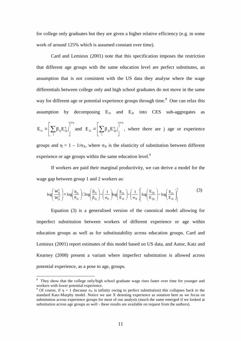
Card and Lemieux (2001) note that this specification imposes the restriction

that different age groups with the same education level are perfect substitutes, an

assumption that is not consistent with the US data they analyse where the wage

differentials between college only and high school graduates do not move in the same

way for different age or potential experience groups through time.8 One can relax this

assumption by decomposing E1t and E2t into CES sub-aggregates as

1/η

j

η

1jt1j1t EβE

= ∑ and

1/η

j

η

2jt2j2t EβE

= ∑ , where there are j age or experience

groups and η = 1 – 1/σX, where σX is the elasticity of substitution between different

experience or age groups within the same education level.9

If workers are paid their marginal productivity, we can derive a model for the

wage gap between group 1 and 2 workers as:

−

−

−

+

=

2t

1t

2jt

1jt

X2t

1t

E2j

1j

2t

1t2jt

1jt

E

Elog

E

Elog

σ

1

E

Elog

σ

1

β

βlog

θ

θlog

W

Wlog

(3)

Equation (3) is a generalised version of the canonical model allowing for

imperfect substitution between workers of different experience or age within

education groups as well as for substitutability across education groups. Card and

Lemieux (2001) report estimates of this model based on US data, and Autor, Katz and

Kearney (2008) present a variant where imperfect substitution is allowed across

potential experience, as a pose to age, groups.

8 They show that the college only/high school graduate wage rises faster over time for younger and workers with lower potential experience. 9 Of course, if η = 1 (because σX is infinity owing to perfect substitution) this collapses back to the standard Katz-Murphy model. Notice we use X denoting experience as notation here as we focus on substitution across experience groups for most of our analysis (much the same emerged if we looked at substitution across age groups as well - these results are available on request from the authors).

12

As with the Katz-Murphy model, we can again make the technological

parameters a function of the linear time trend so that the estimating equation becomes

the following:

jt2t

1t

2jt

1jt3

2t

1t210

2jt

1jt

E

Elog

E

Elog

E

Elog t

W

Wlog v+

−

+

++=

δδδδ

(4)

where the coefficient on the trend δ1 indicates the relative demand shift over and

above supply changes, δ2 = -1/σE, δ3 = -1/σX and v is an error term.10

Estimates of Supply-Demand Models

We present estimates of the Katz-Murphy (KM) and Card-Lemieux (CL)

specifications (respectively equations (2) and (4) above) in Table 3. Our time series is

too short to undertake a rigorous analysis for the GB data, so this part of the analysis

only considers the US. The dependent variable (as in other papers in the literature) is

a composition-adjusted relative wage11, with the relevant relative wage under

consideration in different models defined in the Table. The relative supply variables

also follow the literature showing supply in terms of the relative group of equivalents

(see the Data Appendix for more detail).

We begin by discussing estimates of equation (2) and (4) for the wage

differential considered in the vast majority of work - the college only/high school

relative wage - and for college equivalent versus high school equivalent supply. The

10 In practice, the equation from the two-level nested CES model is estimated as a two step procedure. First, the coefficient δ3 can be estimated from regressions of the relative wages of different experience/age groups to their relative supplies to derive a first estimate of σX and a set of efficiency parameters (the β1's and β2's in the CES sub-aggregates) can be obtained for each education group from a regression of wages on supply including experience/age fixed effects and time dummies. Given these, one can then compute E1t and E2t to obtain a model based estimate of aggregate supply. See Card and Lemieux (2001) for more detail. 11 The composition adjustment is described in the Data Appendix. Essentially we take a similar approach to Autor, Katz and Kearney (2008) and estimate predicted fixed weight wage differentials from annual wage regressions disaggregated by gender and the four potential experience groups (i.e. eight separate regressions for each year) controlling for a linear experience variable (and for broad region and race). These wages are then weighted by the hours shares of each group for the whole time period.

13

KM model is specification [1] in the upper panel of the Table and the CL model

(allowing substitutability across age groups within the two skills groups) is

specification [4] in the lower panel of the Table. For the 1963 to 2009 time period

under consideration, the estimates we obtain are similar to those in other work.

First, consider the KM specification [1]. The model uncovers a significant

negative coefficient of -0.347 on the relative supply variable, suggesting an elasticity

of substitution of about 2.9. This is in the same ballpark as Autor, Katz and Kearney's

(2008) estimate of 2.4 for the same data running from 1963 to 2005. Similarly, there

is a significant positive coefficient on the trend variable of 0.014 showing a trend

increase in the college only/high school gap of 1.4 percentage points a year.

Second, consider the CL specification [4]. This specification shows a negative

impact of aggregate supply (with an implied elasticity of substitution of 2.1) and a

significant trend increase of 1.8 percentage points per year. These are different to the

KM model because of the salient feature of the CL model, namely the significant

estimate of σX of 3.7.

As noted above, some authors have remarked that if the same exercise is

carried out for a wage differential defined between college plus (i.e. postgraduates and

college only workers) and high school graduates and the same supply measure that

much the same results follow. One can, of course, test whether that remains the case

for data extended up to 2009. We do so in specifications [2] and [5] in the Table

where we now consider a relative wage as the postgraduate to high school graduate

wage. If the college plus group is homogenous (and the postgraduates and college

only workers can be thought of as perfect substitutes) then one should see the same

estimates as in specifications [1] and [4].

14

Whilst qualitatively similar (i.e. supply depresses wage differentials and there

is a significant trend increase in relative wages over and above supply) the magnitudes

of the estimated effects are rather different. In the KM model, the implied elasticity of

substitution is now 2.3 (as compared to the 2.9 above for college only). Moreover, the

trend coefficient is 50 percent higher at 0.021 compared to 0.014. Both these

postgraduate/college only gaps are statistically significant. The same is true of the CL

model. In specification [5], the estimated impact of aggregate relative supply on

relative wages is more marked than in specification [4], suggesting a slightly lower

substitution elasticity of 1.8 (as compared to 2.1). In addition, the trend coefficient is

larger (at 0.025 vis-à-vis 0.018).

We probe the postgraduate/college only differences more in specifications [3]

and [6]. The specifications here define relative wages as the postgraduate/college only

wage and split the college equivalent supply into postgraduates and college only

equivalents. These estimates are in the spirit of the tests introduced by Ottaviani and

Peri (2011) on whether skill groups can be grouped together or not. They argue that

supply should have no impact if they can be grouped together (implying an infinite

elasticity for perfect substitution).12

In both the KM and CL models, we reject the hypothesis of a zero supply

effect and therefore perfect substitutability. The estimated coefficient on the aggregate

supply variable is negative and significant in both cases, implying an elasticity of

substitution of 7.4 for both the KM and CL models. Interestingly, in the latter case

there is no evidence at all of substitution across experience groups, hence the reason

12 There are other papers in the immigration literature taking a similar approach of testing for substitution of different worker types in relative wage equations derived from nested CES production functions. For the US see Aydemir and Borjas (2007) and for Britain see Manacorda, Manning and Wadsworth (2011).

15

why the KM and CL models yield the same substitution elasticities. This is also borne

out by the significant coefficient on the trend variable, showing an annual increase in

relative wages over and above supply of 0.5 percentage points per year or

cumulatively around a 24 percentage points increase over the full 47 years.

Thus, we decisively reject the null hypothesis of adding together postgraduate

and college only workers. Below we consider some reasons for this, looking in more

detail at differences in the skills and occupations of the two groups of graduates. In

addition, it is worth noting that the similarity of the KM and CL estimates emerges

since relative wages do not show strongly different patterns for low versus high

experience (or younger versus older) workers. This is shown in Figure 3 where there

are similar trends in the composition adjusted postgraduate/college only relative wage

across higher and lower experience groups.

Modelling Aggregate Demand Shifts in the KM and CL Models

So far, we have proxied demand shifts in the KM and CL supply and demand

models via a linear trend. This has been standard practice in existing work. However,

various authors have noted that it has proven harder over time for the model to

produce a good fit. Some authors (Autor, Katz and Kearney, 2008; Goldin and Katz,

2008) have therefore generalised the model, looking at trend non-linearities or trend

breaks. The CL approach also speaks to this, by emphasising the need to consider

changing college only/high school graduate wage differentials across age or

experience cohorts.13

13 Carneiro and Lee (2011) argue that changes in the average quality of college graduates needs to be factored in - when they do so, they argue that the composition (i.e. quality) adjusted college only/high school premium rises by more over time. For more discussion of compositional changes and changing wage inequality see also Lemieux (2006b).

16

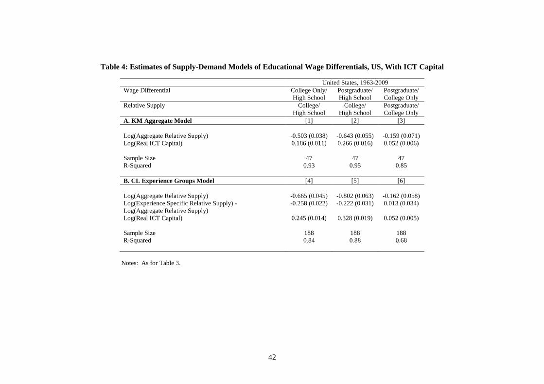
Table 4 takes a different approach, replacing the trend with a technology

proxy, the log of the real ICT capital stock. Interestingly, this produces results more

like the original work, with more negative aggregate supply effects than for the trend

models in Table 3. In the Katz and Murphy (1992) paper based upon data from 1963

to 1987, (1/σE) was estimated at 0.7, leading to the much quoted estimate of σE = 1.4.

In specification [4], now based on the longer time period from 1963 to 2009, the CL

model augmented by the real ICT capital variable estimates (1/σE) for the college

only/high school graduate wage as 0.67, producing an estimate of σE = 1.5, which is

very close to the original Katz-Murphy elasticity.

For our interest in postgraduates, both the KM and CL models incorporating

the real ICT capital variable corroborate the findings from before and, if anything, are

stronger. The Ottaviani-Peri (2011) type test in specifications [3] and [6] strongly

rejects the hypothesis of constant wage evolutions for postgraduates and college only

graduates. Moreover, the strong and significant coefficient on the real ICT measure

suggests that, over time, demand has been shifting strongly in favour of postgraduate

relative to college only workers.

Thus, over the last five decades in the US, relative demand seems to have

shifted over time in favour of postgraduate workers as compared to college only

workers. Moreover, the two groups of workers appear to be imperfect substitutes in

production so that rising wage gaps between postgraduate and college only workers

have been an important aspect of rising within-group inequality amongst graduates

that has, to date, been rather under-studied by the literature.

17

4. Connections to Changes in Industry Computerization

A large body of existing research connects the relative demand shifts underpinning

increased wage inequality to observable measures of technology, usually relating the

two through industry-level regressions.14 This work reports that technology measures

like R&D, innovation, computer usage and investment in computers have been

strongly correlated with the increased demand for more educated workers, therefore

being important drivers of the long run secular demand increases we have already

described earlier in the paper.

In this section, we report results where within-industry changes in relative

labour demand for five education groups are related to changes in computerization,

with a particular focus on looking what has happened in the 2000s as the earlier

studies do not extend into this decade and continuing the focus on what is going on

within the graduate group with respect to postgraduates and college only workers.15

Industry Computerization and Skill Demand

We begin by estimating the following long run within-industry relationship

between changes in relative labour demand, S, and changes in computer use, C, as:

1ejtωj∆C1eγ1eλejt∆S ++= (5)

where ejτSejtSejt∆S −= is change in the employment share for education group e in

industry j between years τ and t (in the US between 1989 and 2008, and for GB

14 The seminal article is Berman, Bound and Griliches (1994) which related changes in the demand for skilled labour in US manufacturing industries to measures of R&D and computer investment. Autor, Katz and Krueger (1998) study connections with industry computerization in detail, and Berman, Bound and Machin (1998) and Machin and Van Reenen (1998) offer cross-country comparisons based on the same industries across countries. The literature, including reference to more studies, is reviewed in Katz and Autor (1999). 15 In their US study, Autor, Katz and Krueger (1998) look at four education groups: college, some college, high school graduates and less than high school. Given our focus on heterogeneity in the college group, we split that into postgraduates and college only, so as to look at five groups. We also study five (broadly comparable groups) in the GB data: postgraduates, college only, intermediate 1, intermediate 2 and no qualifications (see the Data Appendix for definitions).

18

between 1996 and 2008) and ∆Cj is the change in the proportion of workers in

industry j using a computer at work between 1984 and 2003 for the US (from the

October Current Population Survey Supplements) and between 1992 and 2006 for GB

(from the 1992 Employment in Britain and the 2006 Skills Survey).

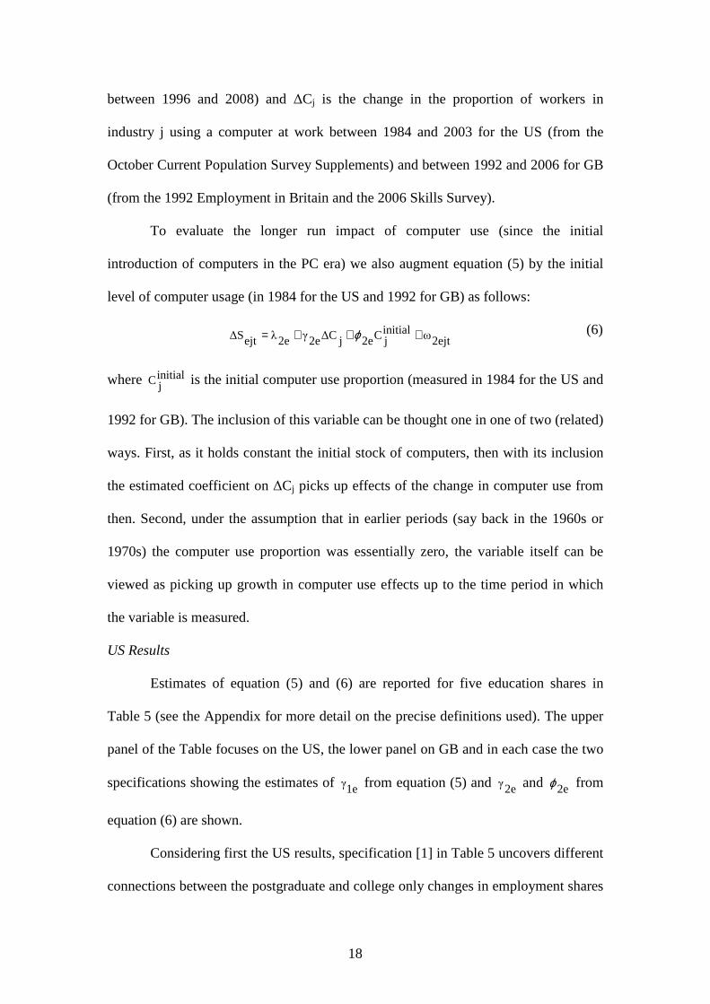
To evaluate the longer run impact of computer use (since the initial

introduction of computers in the PC era) we also augment equation (5) by the initial

level of computer usage (in 1984 for the US and 1992 for GB) as follows:

2ejtωinitialjC2ej∆C2eγ2eλejt∆S +++= ϕ (6)

where initialjC is the initial computer use proportion (measured in 1984 for the US and

1992 for GB). The inclusion of this variable can be thought one in one of two (related)

ways. First, as it holds constant the initial stock of computers, then with its inclusion

the estimated coefficient on ∆Cj picks up effects of the change in computer use from

then. Second, under the assumption that in earlier periods (say back in the 1960s or

1970s) the computer use proportion was essentially zero, the variable itself can be

viewed as picking up growth in computer use effects up to the time period in which

the variable is measured.

US Results

Estimates of equation (5) and (6) are reported for five education shares in

Table 5 (see the Appendix for more detail on the precise definitions used). The upper

panel of the Table focuses on the US, the lower panel on GB and in each case the two

specifications showing the estimates of 1eγ from equation (5) and 2eγ and 2eϕ from

equation (6) are shown.

Considering first the US results, specification [1] in Table 5 uncovers different

connections between the postgraduate and college only changes in employment shares

19

and changes in computer use. Indeed, the positive connection reported in earlier work

(e.g. Autor, Katz and Krueger, 1998) is only present for the postgraduate group. It

seems that the connections between industry changes in skill demand and changes in

computerization are not neutral across the two groups of college graduates.

Considering the three other education groups (some college, high school

graduates and high school drop outs), we uncover the same pattern as seen in the

earlier work, namely that the main losers from increased computerization are the high

school graduates (not the dropouts). This, of course, is consistent with

computerization playing a significant role in the polarization of skill demand (where

jobs were hollowed out and/or relative wages deteriorated in the middle part of the

education distribution).16

The second US specification [2] in Table 5 shows estimates of equation (6)

which additionally include the 1984 computer use proportion. This sheds more light

on what has been going on within the graduate group. The change in the postgraduate

wage bill share is significantly related to both the 1984 to 2003 increases in industry

computerization and to the 1984 level. On the other hand, the change in the college

only wage bill share is insignificantly related to the 1984 to 2003 change and

positively and significantly only to the initial 1984 level. Thus, the initial influx of

computers to industries benefited both groups, but thereafter the group of graduates

who benefited was confined to those with a postgraduate qualification. This paints a

rather different picture as to who benefited most from the computer revolution. It

seems initially that labour demand shifted in favour of all graduates, but as time

16 For evidence on labour market polarization in the US see Autor, Katz and Kearney (2008), in the UK see Goos and Manning (2008) and for Germany see Spitz-Oener (2006) or Dustmann et al. (2009). Goos, Manning and Solomons (2009) and Michaels, Natraj and Van Reenen (2010) present evidence that polarization connected to computerization is pervasive across a number of countries.

20

progressed labour demand tilted more in favour of postgraduates. This suggests that

more recently postgraduates possess skills that make them more complementary to

computers, a point we return to towards the end of this section where we look directly

at differences in the skills of postgraduate and college only workers.

It is worth benchmarking the within-college group differences for

postgraduates and college only with the earlier work where the overall college share

(i.e. the sum of the two shares) was used as dependent variable. If we put them

together in one college plus group as in the earlier work, we obtain a coefficient (and

associated standard error) of 0.131 (0.031) on the 1984 to 2003 ∆Cj variable and of

0.010 (0.001) on the 1984 initialjC variable. Thus, like the earlier work, there is indeed a

strong connection between changes in college plus employment shares and computers,

but our findings highlight that it is one characterised by non-neutrality of technology-

skill complementarity across the postgraduate and college only groups.

GB Results

The lower panel of Table 5 gives the GB results. Consider specification [3]

first. As with the US findings, we find non-neutrality amongst the two groups of

graduates. We obtain a significant positive coefficient on the postgraduate variable

and an insignificant (positive) one on the college only variable. The same is true in

specification [4] when the initial computer usage variable (measured in 1992) is

included. Here though, it is evident that there are strong and significant connections

between changes in the postgraduate employment share and both changes in industry

computerization and the 1992 level of computer usage. On the other hand,

connections with the college only share are not statistically significant.

21

For the other three education groups, the results also confirm that the British

labour market was also characterised by polarization connected to industry

computerization and its associations with changes in the relative wages and

employment of workers with different education levels. The hollowing out of the

middle is seen in the results reported in the Table where the intermediate qualification

groups fare worst, whilst those at each end of the education spectrum (the

postgraduates at the top and the no qualifications group at the bottom) have the best

outcomes in relative terms.

Sub-Period Analysis and Complex/Basic Computer Use

The notion that increased computer usage acts as a measure of new technology

over the whole time period we consider also requires some discussion (see Beaudry,

Doms and Lewis, 2010, who critically appraise the extent to which the widespread use

of personal computers reflects a technological revolution). This is a potentially

important aspect of our analysis in that we look at changes in computer usage between

1984 and 2003 as, by 2003, in some industries the percentage of workers using a

computer is high. This possible near reaching of a ceiling, of course, shows the need

to control for initial levels of computer usage in the regressions. It also raises the

question of whether changes in a simple headcount measure of any computer use at

work adequately reflect technological change.

We consider this question in two ways for the US analysis (sample size issues

precluded a similar analysis being undertaken for GB). First, we break down the

analysis into two sub-periods. These are dictated by the availability of computer usage

data in the CPS in the October supplements of 1984, 1993 and 2003. We thus look at

changes in employment shares between 1998 and 2008 and how they relate to changes

in computer usage between 1993 and 2003, and perform the same sub-period split for

22

changes in employment shares between 1989 and 1998 with computer use changes

measured from 1984 to 1993.17

Estimates of equation (6) are reported in specifications [1] and [2] of Table 6

for these two sub-periods. The analysis essentially corroborates the earlier findings

where there is a stronger computerization effect for postgraduates than for college

only workers. A closer inspection of the results does, however, reveal that this more

true of the first sub-period (in specification [1]). In the second sub-period

(specification [2]) the postgraduate and college only computerization effects are more

similar.

To further probe this question, the second way we consider the usefulness of

the computer usage data to measure technological change is by breaking down the

computerization measure into whether the computer is used for complex or basic

tasks. For the second period of data we can do this since the 1993 and 2003 computer

use supplements in the CPS report whether computers are used for more complex

tasks like programming as well as for a variety of other more basic purposes (see the

Data Appendix for more detail). We therefore define complex use as computer

programming and basic use as all other computer use.

Specification [3] of Table 6 reports the results. It is evident that the changes in

complex computer usage are strongly associated with the increased demand for

postgraduates. Both the change and the initial level of complex computer usage have

17 The second period closely approximates the time period studied by Autor, Katz and Krueger (1998). Autor, Katz and Krueger report an estimated coefficient (standard error) of 0.152 (0.025) on the computer use variable in a regression of changes in college plus employment shares between 1979 and 1993 on the 1984 to 1993 change in computer usage for 191 US industries. Running the same regression (i.e. not including the initial level of computer usage) on our 215 industries for the change in college plus employment shares between 1989 and 1998 we obtain a very similar estimate of 0.144 (0.026) on the 1984 to 1993 change in computer use variable. For this specification, considering postgraduate and college only shares separately produces a coefficient (standard error) of 0.087 (0.015) on the change in computer use variable in a change in postgraduate share equation and of 0.057 (0.023) in a change in college only share equation.

23

a positive and significant impact on the change in the postgraduate share of

employment. The same is not true of the college only group, where it is changes in

basic computer usage that are significantly related to increased employment of this

group of workers.

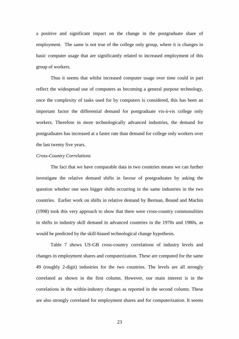
Thus it seems that whilst increased computer usage over time could in part

reflect the widespread use of computers as becoming a general purpose technology,

once the complexity of tasks used for by computers is considered, this has been an

important factor the differential demand for postgraduate vis-à-vis college only

workers. Therefore in more technologically advanced industries, the demand for

postgraduates has increased at a faster rate than demand for college only workers over

the last twenty five years.

Cross-Country Correlations

The fact that we have comparable data in two countries means we can further

investigate the relative demand shifts in favour of postgraduates by asking the

question whether one sees bigger shifts occurring in the same industries in the two

countries. Earlier work on shifts in relative demand by Berman, Bound and Machin

(1998) took this very approach to show that there were cross-country commonalities

in shifts in industry skill demand in advanced countries in the 1970s and 1980s, as

would be predicted by the skill-biased technological change hypothesis.

Table 7 shows US-GB cross-country correlations of industry levels and

changes in employment shares and computerization. These are computed for the same

49 (roughly 2-digit) industries for the two countries. The levels are all strongly

correlated as shown in the first column. However, our main interest is in the

correlations in the within-industry changes as reported in the second column. These

are also strongly correlated for employment shares and for computerization. It seems

24

that it is the same industries in the two countries that had faster increases in computer

usage and, at the same time, shifts in relative demand towards postgraduates. The

correlations are strong (with p-values showing statistical significance levels of better

than 1 percent in all cases). Figure 4 plots US versus GB changes in postgraduate

employment shares and changes in computer usage and fits a regression line through

them, showing these strong cross-country correlations.

Cost Share Equations

So far, we have considered shifts in relative labour demand by education

group and how they have been related to changes in computerization across industries

over time. The advantage of our analysis so far was that we were able to do this for

around 215 US industries and 51 GB industries covering the whole economy.

A common approach adopted in some of the literature has been to estimate

more detailed cost share equations derived directly from a translog cost function.

These relate changes in cost shares by education group to technology indicators and

also to industry capital and output. Thus, one can explore the extent of capital-skill

complementarity/substitution and of technology-skill complementarity/substitution.

We have also considered this approach, albeit implementing for a more aggregated set

of industries owing to the need for capital and output data.18

The cost share equation we estimate takes the form

3ejtω∆logYπ∆logKφj(CI/Y)3eγ3eλejt∆WB jtejte ++++= (7)

where ejt∆WB is the within-industry change in the wage bill share of education group

e, CI/Y is the share of ICT investment in value added, K is the net capital stock and Y

18 The need for capital stock data in service sector industries (which we obtain from the US National Income and Product Accounts, NIPA and for GB from the EU KLEMS data) also means we have to lose some industries from our analysis where capital data is not well measured for public sector industries (as in Autor, Katz and Krueger, 1998, we are forced to omit education and health from this analysis).

25

is value added. Variants of equation (7) have been estimated in the literature exploring

capital-skill complementarities (dating back to Griliches, 1969) and more recently in

the wage inequality work exploring technology-skill complementarities.

Estimates of equation (7) are given in Table 8 for 52 US industries and 28 GB

industries. Differences in the postgraduate/college only coefficients on the technology

variable are more muted, but they are supportive of the pattern seen earlier in the

relative labour demand equations. Industries with more ICT investment saw faster

increases in wage bill shares for postgraduates than for college only workers, which is

indicative of non-neutrality between the two groups of college graduates. There is also

significant hollowing out in the middle part of the distribution with some college and

high school graduates in the US (intermediate 1 and intermediate 2 in GB) faring

worst.

What Are The Skills That Make Postgraduates More in Demand Than College Only

Graduates?

An obvious question that emerges from our analysis to date asks what are the

skills possessed by postgraduates that make them imperfect substitutes for college

only workers? We can shed more light on this by looking at the British 2006 Skills

Survey that contains information on education levels of workers, but also on their

specific skills in terms of the job tasks done by workers.

Table 9 shows postgraduate/college only differences in cognitive skills,

problem solving skills, people skills, firm-specific skills, the tasks they use computers

for and the routineness of their job. Most of the numbers in the Table (with the

exception of the proportions using computers) are based on a scale of 1-5 (5 being

highest) from questions on task performance asking 'How important is this task in

26

your current job?', with 1 denoting 'not at all important', 2 'not very important', 3

'fairly important', 4 'very important' and 5 'essential'.

It is clear that both sets of graduates do jobs with high skill and job task

requirements. However, in almost all cases the levels are higher (and significantly so)

for postgraduates. For example, postgraduates have higher numeracy levels

(especially advanced numeracy), higher levels of analysing complex problems and

specialist knowledge or understanding. The computer usage breakdowns are also

interesting, showing clearly that postgraduates and college only workers have high

levels of computer usage, but that using computers to perform complex tasks is

markedly higher amongst the postgraduate group.

We view the Table 9 material as clearly confirming that postgraduates do

possess different skills and do jobs involving different (usually more complex) tasks

than college only workers. This is in line with the earlier analyses showing them to be

imperfect substitutes and with the notion that relative demand has shifted faster in

favour of the postgraduate group within the group of all college graduates. As such,

this appears to be an important aspect of rising wage inequality amongst college

graduates.

5. Postgraduate Heterogeneity

The analysis so far has considered whether workers have any postgraduate

qualifications. This is the only measure available for the longer time periods we

consider. However, from 1992 onwards in the US, and from 1996 onwards in Britain,

we do have consistent data on what type of broad postgraduate qualification people

hold. We can thus consider the evolution of employment shares and relative wages

27

within the postgraduate group for people with Master’s degrees, doctorates and other

postgraduate qualifications.

Employment Changes by Type of Postgraduate Qualification

Table 10 shows the employment share and share amongst postgraduates of

these three qualification groups, from 1992 to 2009 in the upper panel for the US, and

from 1996 to 2009 in the lower panel for GB. In both countries, the biggest share is

for Master’s degrees, and this is the group seeing the larger increase in relative

supply. In the US, the share of Master’s rises, whilst the share of professional

qualifications falls, and the share of doctorates remains relatively constant. In Britain,

the Master’s share goes up, with the professional degree group staying constant and

the share of postgraduates with a PhD falling.

Wage Changes by Qualification

Table 11 considers the evolution of wage differentials for those with Master’s

degrees and doctorates as compared to workers with just a college degree.19 The

wage differentials rise over the period considered for Master’s and doctorates in both

countries, but by more in the latter case as shown in the final rows of the two panels

which shows the relative Doctoral/Master's degree gaps over the three years.

Using similar methods to those used earlier in the paper, Figure 5 graphs the

trends in the composition-adjusted postgraduate wage differentials for those with

Master’s degrees and doctorates again relative to those with college only

qualifications. For both countries, these clearly fan out through time. The doctorates

are pulling away from the Master's qualifications in terms of pay, showing within

post-graduate qualification increasing inequality.

19 The composition of the professional degree group differs substantially across the two countries since they consist largely of professionals in the US whereas in Britain a substantial number are those with post-graduate teaching qualifications.

28

Which Occupations do Postgraduates and College Only Workers do?

The final aspect of the extent to which postgraduate and college only workers

differ that we consider is to look in which occupations they are employed. Table 12

shows the top five occupations in terms of their share in employment for college only,

Master's and doctorate degrees for 2010 for the US (in the upper panel) and for GB (in

the lower panel).

There are several interesting features of the top five occupations of these three

groups of workers. First, the top five tend to be different occupations in both

countries. Second, whilst the occupational categories are not quite the same across

countries, there are some clear similarities. Third, the postgraduate occupations are

more segregated than the college only. For postgraduates, in the US the top five (out

of 497 occupations) account for almost half of employment (49 percent) and in GB

(out of 353 occupations) for around 45 percent. The college only distribution is a lot

more dispersed, with the top 5 accounting for 16 percent of employment in the US

and for 20 percent in GB.20

Table 13 considers how the extent of occupational clustering differs across the

different types of graduates. It shows the number of occupations that respectively

have college only, Master's and doctorate degree workers, and a Gini coefficient

measuring how concentrated into occupations are these groups of graduates. The

numbers in the Table make it clear that the extent of occupational clustering is

different for the three groups. College only workers are spread more widely across the

occupational structure and the occupational distribution of postgraduates is more

20 Benson (2011) considers the spatial distribution of occupations in the US by education group. Whilst not the main focus of his analysis, he shows the occupational structure of postgraduates to be more segregated than for college only workers (and indeed for the rest of the labour force).

29

segregated. Within the two groups of postgraduates, the doctorate holders are

occupationally more segregated than are those individuals with a Master's degree.

Thus, we see differences in the occupational structure of employment for the

postgraduate group vis-à-vis college only graduates. This is consistent with and offers

additional corroborative evidence relevant to our earlier findings of less than perfect

substitution and in trend differences in relative wages that have differed between the

postgraduate and college only group.

6. Conclusions

In this paper, we focus on what has to date been a rather neglected, but what is

becoming an increasingly important, development of the education structure of the

workforce that has been occurring in many countries. We offer new evidence on how

the changing education structure has contributed to rising wage inequality in the

United States and Great Britain. Our main focus is on increasing divergences within

the group of workers who go to university. We document that there have been

increases through time in the number of workers with a postgraduate qualification.

We show that, at the same time as this increase in their relative supply, their relative

wages have strongly risen as compared to workers with only a college degree.

Consideration of shifts in their demand and supply uncovers trend increases in

relative demand for postgraduates that are a key driver of increasing within-graduate

inequality and of overall rises in inequality. In line with these shifts in relative

demand, we report various pieces of evidence in line with the notion that postgraduate

workers and college only workers are different, in that they are not perfect substitutes,

as they possess skills that have a higher value in the labour market and that they work

in different occupations.

30

The relative demand shifts in favour of workers with postgraduate

qualifications are strongly correlated with technical change as measured by computer

usage and investment. In fact, it turns out that, over the years when computers have

massively diffused into workplaces, the principal beneficiaries of this computer

revolution has not been all graduates, but those with postgraduate qualifications. As

such, there has been a strong connection between the increased presence of

postgraduate workers in the labour force and rising graduate wage inequality over

time.

31

References

Acemoglu, D. and D. Autor (2010) Skills, Tasks and Technologies: Implications for Employment and Earnings, in Ashenfelter, O. and D. Card (eds.) Handbook of Labor Economics Volume 4, Amsterdam: Elsevier.

Autor, D., L. Katz and A. Krueger (1998) Computing Inequality, Quarterly Journal of

Economics, 113, 1169-1213. Autor, D., L. Katz, and M. Kearney (2008) Trends in U.S. Wage Inequality: Re-

Assessing the Revisionists, Review of Economics and Statistics, 90 300-323. Aydemir, A. and G. Borjas (2007) Cross-Country Variation in the Impact of

International Migration: Canada, Mexico, and the United States, Journal of the European Economic Association, 5, 663-708.

Beaudry, P., M. Doms and E. Lewis (2010) Should the Personal Computer Be

Considered a Technological Revolution? Evidence from U.S. Metropolitan Areas, Journal of Political Economy, 118, 988-1036.

Berman, E., J. Bound and Z. Griliches (1994) Changes in the Demand for Skilled

Labor Within U.S. Manufacturing Industries: Evidence from the Annual Survey of Manufacturing, Quarterly Journal of Economics, 109, 367–98.

Berman, E., J. Bound and S. Machin (1998) Implications of Skill-Biased

Technological Change: International Evidence, Quarterly Journal of Economics, 113, 1245-1280.

Benson, A. (2011) A Theory of Dual Job Search and Sex-Based Occupational

Clustering, MIT mimeo. Card, D. and T. Lemieux (2001) Can Falling Supply Explain the Rising Return to

College for Younger Men? A Cohort-Based Analysis, Quarterly Journal of Economics, 116, 705-46.

Carneiro, P. and S. Lee (2011) Trends in Quality-Adjusted Skill Premia in the United

States, 1960-2000, American Economic Review, forthcoming. Devereux, P. and W. Fan (2011) Earnings Returns to the British Education

Expansion, Economics of Education Review, forthcoming. Dustmann, C., J. Ludsteck and U. Schoenberg (2009) Revisiting the German Wage

Structure, Quarterly Journal of Economics, 124, 843-81. Eckstein, Z. and E. Nagypal (2004) The Evolution of US Earnings Inequality: 1961-

2002, Federal Reserve Bank of Minneapolis Quarterly Review, 28, 10–29 Goldin, C. and L. Katz (2008) The Race Between Education and Technology,

Harvard University Press.

32

Goos, M. and A. Manning (2007) Lousy and Lovely Jobs: The Rising Polarization of Work in Britain, Review of Economics and Statistics, 89, 118-33.

Goos, M., A. Manning and A. Salomons (2009) The Polarization of the European

Labor Market, American Economic Review, Papers and Proceedings, 99, 58-63.

Griliches, Z. (1969) Capital-Skill Complementarity, Review of Economics and

Statistics, 51, 465-8. Katz, L. and D. Autor (1999) Changes in the Wage Structure and Earnings Inequality,

in O. Ashenfelter and D. Card (eds.) Handbook of Labor Economics, Volume 3, North Holland.

Katz, L. and K. Murphy (1992) Changes in Relative Wages, 1963-87: Supply and

Demand Factors, Quarterly Journal of Economics, 107, 35-78. Lemieux, T. (2006a) Postsecondary Education and Increasing Wage Inequality,

American Economic Review, Papers and Proceedings, 96, 195-99. Lemieux, T. (2006b) Increased Residual Wage Inequality: Composition Effects,

Noisy Data or Rising Demand for Skill, American Economic Review, 96, 461-98.

Machin, S. (2011) Changes in UK Wage Inequality Over the Last Forty Years, in P.

Gregg and J. Wadsworth (eds.) The Labour Market in Winter - The State of Working Britain 2010, Oxford University Press.

Machin, S. and J. Van Reenen (1998) Technology and Changes in Skill Structure:

Evidence From Seven OECD countries, Quarterly Journal of Economics, 113, 1215-44.

Machin, S. and A. Vignoles (2005) What's the Good of Education?, Princeton

University Press. Manacorda, M., A. Manning and J. Wadsworth (2011) The Impact of Immigration on

the Structure of Male Wages: Theory and Evidence From Britain, Journal of the European Economic Association, forthcoming.

Michaels, G. A. Natraj and J. Van Reenen (2010) Has ICT Polarized Skill Demand?

Evidence from Eleven Countries over 25 years, National Bureau of Economic Research Working Paper 16138.

Ottaviani, G. and G. Peri (2011) Rethinking the Effects of Immigration on Wages,

Journal of the European Economic Association, forthcoming. Spitz-Oener, A. (2006) Technical Change, Job Tasks and Rising Educational

Demands: Looking Outside the Wage Structure, Journal of Labor Economics, 24, 235-70.

33

Timmer, M., T. Van Moergastel, E. Stuivenwold, G.Ypma, M. O’Mahony and M. Kangasniemi (2007) EU KLEMS Growth and Productivity Accounts Version 1.0, University of Groningen Mimeo.

Tinbergen, J. (1974) Substitution of Graduate by Other Labour, Kyklos, 27, 217-26. Walker, I. and Y. Zhu (2008) The College Wage Premium and the Expansion of

Higher Education in the UK, Scandinavian Journal of Economics, 110, 695-709.

34

Figure 1: Trends in Overall 90-10 Wage Ratio

United States, 1963 to 2009

11.

21.

41.

6F

T L

og 9

0/10

Ra

tio

1963 1970 1975 1980 1985 1990 1995 2000 2005 2009Year

Men Women

Great Britain, 1970 to 2009

.8.9

11.

11.

21.

3F

T L

og 9

0/10

Rat

io

1970 1975 1980 1985 1990 1995 2000 2005 2009Year

Men Women

Notes: US 90-10 Log(Earnings) ratios from March Current Population Surveys for income years 1963 to 2009. Weekly earnings for full-time full year workers. GB 90-10 Log(Earnings) ratios from 1970 to 2010 from the New Earnings Survey/Annual Survey of Hours and Earnings. Weekly earnings for full time workers.

35

Figure 2: Trends in 90-10 Wage Ratio For Graduates

United States, 1963 to 2009

.91.

11.

31.

5Lo

g E

arni

ngs

Rat

io

1963 1970 1975 1980 1985 1990 1995 2000 2005 2009Year

Men Graduates Women Graduates

Great Britain, 1977 to 2009

.81

1.2

1.4

Log

Ear

ning

s R

atio

1977 1980 1985 1990 1995 2000 2005 2009Year

Men Graduates Women Graduates

Notes: US 90-10 Log(Earnings) ratios from March Current Population Surveys for income years 1963 to 2009. Weekly earnings for full-time full year workers. GB 90-10 Log(Earnings) ratios from 1977 to 2009 from splicing together the General Household Survey (1977-1992) to the Labour Force Survey (1993 to 2009). Weekly earnings for full time workers (those working 30 or more hours).

36

Figure 3: Trends in Composition Adjusted Postgraduate

Wage Differentials by Experience Group

Postgraduate/College Only - United States, 1963 to 2009

0.1

.2.3

Tre

nds

in W

age

Diff

eren

tials

1963 1970 1975 1980 1985 1990 1995 2000 2005 2009Year

PG/College, 0-9 PG/College, 10-19PG/College, 20-29 PG/College, 30-39

Notes: Composition adjusted log relative wage differentials by experience group computed from March CPS data for full-time full-year workers aged 26-60.

37

Figure 4: Cross-Country Correlations in Within-Industry Changes in

Postgraduate Shares and Computer Usage (49 Industries)

Postgraduate Employment Shares

0.0

02.0

04.0

06A

nnua

lised

Cha

nge

in P

G S

hare

in E

mpl

oym

ent,

US

0 .0025 .005 .0075 .01 .0125Annualised Change in PG Share in Employment, GB

Correlation = 0.65, P-Value = 0.00

Computer Usage

.005

.01

.015

.02

.025

.03

Ann

ualis

ed C

hang

e in

Com

pute

r U

se, U

S

0 .005 .01 .015 .02 .025 .03 .035 .04 .045Annualised Change in Computer Use, GB

Correlation = 0.58, P-Value = 0.00

Notes; Based on the same 49 industries across the two countries.

38

Figure 5: Composition Adjusted Wage Differentials by Postgraduate Qualification

United States, 1992 to 2009

.1.2

.3.4

Tre

nds

in P

ostg

radu

ate

Wag

e D

iffer

entia

ls

1992 1995 2000 2005 2009Year

Master's/College Doctorate/College

Great Britain, 1996 to 2009

.05

.1.1

5.2

.25

Tre

nds

in P

ostg

radu

ate

Wag

e D

iffer

entia

ls

1996 2000 2005 2009Year

Master's/College Doctorate/College

Notes: Composition adjusted log relative wage differentials computed from March CPS (US) and Labour Force Survey (GB) data for full-time full-year workers aged 26-60.

39

Table 1: Employment Shares by Education

United States

1963 1970 1980 1990 2000 2009

College Degree or Higher 0.137 0.158 0.238 0.277 0.316 0.359 Postgraduate Degree 0.037 0.046 0.075 0.089 0.106 0.127 College Degree Only 0.100 0.112 0.164 0.189 0.209 0.232 Postgraduate Share 0.268 0.290 0.313 0.320 0.337 0.354

Great Britain

1996 2000 2009 College Degree or Higher 0.145 0.180 0.289 Postgraduate Degree 0.044 0.057 0.107 College Degree Only 0.101 0.123 0.182 Postgraduate Share 0.301 0.315 0.370

Notes: Source for United States is March Current Population Surveys. Source for Great Britain is Labour Force Surveys. Employment shares are defined for people in work with 0 to 39 years of potential experience and aged 26 to 60.

40

Table 2: Wage Differentials by Education

United States 1963 1970 1980 1990 2000 2009

College Degree or Higher 0.337

(0.011) 0.416

(0.008) 0.384

(0.007) 0.529

(0.006) 0.628

(0.008) 0.680

(0.006) Postgraduate Degree 0.338

(0.020) 0.455

(0.013) 0.470

(0.010) 0.641

(0.009) 0.768

(0.010) 0.858

(0.008) College Degree Only 0.337

(0.012) 0.402

(0.009) 0.344

(0.007) 0.476

(0.007) 0.555

(0.008) 0.581

(0.007) Postgraduate Degree Versus College Degree Only 0.001

(0.021) 0.053

(0.014) 0.125

(0.010) 0.165

(0.010) 0.214

(0.011) 0.277

(0.008) Sample Size 12100 23217 29546 34944 29436 43394 Great Britain 1996 2000 2009 College Degree or Higher 0.468

(0.007) 0.470

(0.007) 0.498

(0.007) Postgraduate Degree 0.504

(0.015) 0.540

(0.010) 0.574

(0.011) College Degree Only 0.451

(0.011) 0.435

(0.008) 0.451

(0.008) Postgraduate Degree Versus College Degree Only 0.052

(0.017) 0.104

(0.011) 0.123

(0.011) Sample Size 20072 36590 27280

Notes: Source for United States is March Current Population Survey. Source for Great Britain is 1996, 2000 and 2009 Labour Force Surveys. Full time full-year workers with 0 to 39 years of potential experience and aged 26 to 60 in the US; full time workers with 0 to 39 years of potential experience and aged 26 to 60 in GB. Wage differentials relative to high school graduates in the US and intermediate qualifications in GB. Control variables included are: gender, experience, experience squared, broad region and race (US); gender, experience, experience squared, London and white. Standard errors in parentheses.

41

Table 3: Estimates of Supply-Demand Models of Educational Wage Differentials, US

United States, 1963-2009 Wage Differential College Only/

High School Postgraduate/ High School

Postgraduate/ College Only

Relative Supply College/ High School

College/ High School

Postgraduate/ College Only

A. KM Aggregate Model [1] [2] [3] Log(Aggregate Relative Supply) -0.347 (0.034) -0.441 (0.040) -0.135 (0.061) Trend 0.014 (0.001) 0.021 (0.001) 0.005 (0.001) Sample Size 47 47 47 R-Squared 0.91 0.96 0.87 B. CL Experience Groups Model [4] [5] [6] Log(Aggregate Relative Supply) -0.466 (0.032) -0.555 (0.043) -0.135 (0.053) Log(Experience Specific Relative Supply) - Log(Aggregate Relative Supply)

-0.271 (0.023) -0.243 (0.029) 0.007 (0.033)

Trend 0.018 (0.001) 0.025 (0.001) 0.005 (0.001) Sample Size 188 188 188 R-Squared 0.86 0.90 0.70

Notes: The dependent variable is the log of the relevant fixed weighted (composition adjusted) wage differentials. Standard errors in parentheses. Four experience specific groups (0-9, 10-19, 20-29, 30-39). The CL models include dummies for experience groups and are estimated using the two step process discussed in footnote 7 of the paper and in Card and Lemieux (2001).

42

Table 4: Estimates of Supply-Demand Models of Educational Wage Differentials, US, With ICT Capital

United States, 1963-2009 Wage Differential College Only/

High School Postgraduate/ High School

Postgraduate/ College Only

Relative Supply College/ High School

College/ High School

Postgraduate/ College Only

A. KM Aggregate Model [1] [2] [3] Log(Aggregate Relative Supply) -0.503 (0.038) -0.643 (0.055) -0.159 (0.071) Log(Real ICT Capital) 0.186 (0.011) 0.266 (0.016) 0.052 (0.006) Sample Size 47 47 47 R-Squared 0.93 0.95 0.85 B. CL Experience Groups Model [4] [5] [6] Log(Aggregate Relative Supply) -0.665 (0.045) -0.802 (0.063) -0.162 (0.058) Log(Experience Specific Relative Supply) - Log(Aggregate Relative Supply)

-0.258 (0.022) -0.222 (0.031) 0.013 (0.034)

Log(Real ICT Capital) 0.245 (0.014) 0.328 (0.019) 0.052 (0.005) Sample Size 188 188 188 R-Squared 0.84 0.88 0.68

Notes: As for Table 3.

43

Table 5: Estimates of the Relationship Between Changes in Employment Shares and Changes in Computer Usage Across Industries

United States, 215 Industries [1] [2] Change in Employment Shares, 1989-2008

Post-Graduates

College Only

Some College

High School Graduates

High School Dropouts

Post-Graduates

College Only

Some College

High School Graduates

High School Dropouts

Change in Computer Use, 1984-2003

0.080 (0.022)

0.005 (0.026)

-0.046 (0.028)

-0.096 (0.036)

0.057 (0.025)

0.105 (0.019)

0.026 (0.025)

-0.080 (0.024)

-0.142 (0.029)

0.090 (0.020)

Computer Use, 1984 0.005 (0.001)

0.004 (0.001)

-0.007 (0.001)

-0.009 (0.001)

0.007 (0.001)

R-Squared 0.06 0.06 0.01 0.02 0.02 0.30 0.12 0.29 0.34 0.36 Great Britain, 51 Industries [3] [4] Change in Employment Shares, 1996-2008

Post-Graduates

College Only

Interm-ediate 1

Interm-ediate 2

No Qualifications

Post-Graduates

College Only

Interm-ediate 1

Interm-ediate 2

No Qualifications

Change in Computer Use, 1992-2006

0.094 (0.039)

0.037 (0.052)

-0.234 (0.057)

0.181 (0.093)

-0.078 (0.043)

0.133 (0.033)

0.055 (0.053)

-0.238 (0.058)

0.088 (0.079)

-0.037 (0.038)

Computer Use, 1992 0.009 (0.002)

0.004 (0.003)

-0.001 (0.003)

-0.021 (0.004)

0.009 (0.002)

R-Squared 0.11 0.01 0.26 0.07 0.06 0.39 0.05 0.26 0.37 0.33

Notes: Standard errors in parentheses. All changes are annualised. US employment shares are from the 1989 and 2008 Merged Outgoing Rotation Groups of the CPS; US computer usage from the 1984 and 2003 October CPS. GB employment shares from the 1986and 2008 LFS; GB computer usage is from the 2006 Skills Survey and the 1992 Employment in Britain.. All regressions weighted by the average employment share in total industry averaged across the two years.

44

Table 6: Sub-Period Analysis and Complex/Basic Computer Use in US Industries

United States, 215 Industries [1] Change in Employment Shares, 1989-1998 Post-Graduates College Only Some College High School Graduates High School Dropouts Change in Computer Use, 1984-1993 0.073

(0.016) 0.029

(0.023) -0.011 (0.025)

-0.144 (0.028)

0.048 (0.018)

Computer Use, 1984 0.003 (0.001)

0.006 (0.001)

-0.005 (0.001)

-0.012 (0.002)

0.007 (0.001)

R-Squared 0.17 0.11 0.07 0.34 0.26 [2] Change in Employment Shares, 1998-2008 Post-Graduates College Only Some College High School Graduates High School Dropouts Change in Computer Use, 1993-2003 0.062

(0.019) 0.053

(0.026) -0.050 (0.028)

-0.084 (0.030)

0.019 (0.021)

Computer Use, 1993 0.005 (0.001)

0.003 (0.001)

-0.007 (0.001)

-0.005 (0.001)

0.004 (0.001)

R-Squared 0.20 0.04 0.20 0.09 0.09 [3] Change in Employment Shares, 1998-2008 Post-Graduates College Only Some College High School Graduates High School Dropouts Change in Complex Computer Use, 1993-2003 0.100

(0.044) 0.040

(0.062) -0.087 (0.065)

-0.083 (0.071)

0.030 (0.050)

Change in Basic Computer Use, 1993-2003 0.065 (0.020)

0.055 (0.028)

-0.052 (0.029)

-0.082 (0.032)

0.014 (0.022)

Complex Computer Use, 1993 0.012 (0.002)

0.004 (0.003)

-0.014 (0.003)

-0.003 (0.003)

0.001 (0.002)

Basic Computer Use, 1993 0.003 (0.001)

0.003 (0.001)

-0.005 (0.001)

-0.005 (0.001)

0.005 (0.001)

R-Squared 0.25 0.05 0.22 0.09 0.13

Notes: Standard errors in parentheses. All changes are annualised. US employment shares are from the 1999 and 2008 Merged Outgoing Rotation Groups of the CPS; US computer usage from the 1993 and 2003 October CPS. Complex computer usage is for programming. Basic computer usage is all other computer use. All regressions weighted by the average employment share in total industry averaged across the two years.

45

Table 7: US-GB Cross-Country Industry Correlations

Levels Within-Industry Changes Employment Shares Postgraduates 0.93 (p = 0.00) 0.65 (p = 0.00) College Only 0.87 (p = 0.00) 0.64 (p = 0.00) Less Than College 0.92 (p = 0.00) 0.59 (p = 0.00) Computerization Computer Use 0.86 (p = 0.00) 0.58 (p = 0.00)

Notes: Pearson correlation coefficients with p-values in parentheses. Based on the same 49 industries across the two countries. Less than college is some college, high school graduates and high school drop outs in the US and intermediate 1, intermediate 2 and no qualifications in GB.

46

Table 8: Estimates of Cost Share Equations

US, NIPA ICT Investment, 52 Industries [1] [2] Change in Wage Bill Shares, 1989-2008

Post-Graduates

College Only

Some College

High School Graduates

High School Dropouts

Post-Graduates

College Only

Some College

High School Graduates

High School Dropouts

CI/Y 0.033

(0.008) 0.028

(0.009) -0.053 (0.009)

-0.041 (0.012)

0.033 (0.009)

0.038 (0.010)

0.023 (0.010)

-0.038 (0.009)

-0.049 (0.013)

0.026 (0.010)

Change in log(K), 1989-2008

0.009 (0.017)

0.030 (0.018)

-0.006 (0.017)

-0.036 (0.024)

0.003 (0.018)

Change in log(Y), 1989-2008

-0.010 (0.009)

0.000 (0.009)

-0.024 (0.008)

0.023 (0.012)

0.011 (0.009)

R-Squared 0.24 0.16 0.41 0.19 0.21 0.26 0.22 0.52 0.26 0.24 GB, KLEMS ICT Fixed Capital Compensation, 28 Industries [3] [4] Change in Wage Bill Shares, 1996-2008

Post-Graduates

College Only

Interm-ediate 1

Interm-ediate 2

No Qualifications

Post-Graduates

College Only

Interm-ediate 1

Interm-ediate 2

No Qualifications

CI/Y 0.041

(0.016) 0.005

(0.012) -0.017 (0.013)

-0.047 (0.022)

0.016 (0.010)

0.052 (0.022)

0.040 (0.014)

-0.016 (0.018)

-0.104 (0.027)

0.028 (0.010)

Change in log(K), 1996-2008

0.006 (0.013)

0.009 (0.008)

-0.012 (0.011)

-0.031 (0.015)

0.028 (0.006)

Change in log(Y), 1996-2008

-0.030 (0.044)

-0.094 (0.028)

0.003 (0.036)

0.160 (0.053)

-0.040 (0.021)

R-Squared 0.21 0.01 0.06 0.15 0.09 0.23 0.35 0.13 0.39 0.54

Notes: Standard errors in parentheses. All regressions weighted by the average wage bill share in total industry averaged across the two years. All changes are annualised. US wage bill shares are from the 1989 and 2008 Merged Outgoing Rotation Groups of the CPS; US computer usage from the 1984 and 2003 October CPS. CI/Y is the share of IT investment in value added. NIPA real IT investment (CI), real non-ICT capital stock (K) and real gross value added (Y) data are for non-residential private fixed assets measured in millions of US dollars in 2005 prices. Real IT investment, real non-ICT capital stock and real gross value added data measured as 5 year averages. The NIPA data are for the private sector only so industries with high government employment (education and health services) are excluded. GB wage bill shares are from the 1996 and 2008 Labour Force Survey; CI/Y is the share of ICT capital formation in value added. Real ICT fixed capital formation (CI), real non-ICT fixed capital compensation (K) and real gross value added (Y) data are from the EU KLEMS data and measured in millions of pounds in 1995 prices. Real capital formation, real non-ICT fixed capital compensation and real gross value added data measured as 5 year averages.

47

Table 9: What Are The Skills and Job Tasks Implying Postgraduates Are More in Demand Than College Only Graduates?

Skill/Job Task Postgraduates College Only Gap (Standard Error) Regression Corrected Gap

(Standard Error) Cognitive Skills Literacy 4.067 3.763 0.304 (0.079) 0.299 (0.079) Simple Numeracy (Basic Arithmetic) 3.606 3.583 0.026 (0.094) 0.023 (0.093) Advanced Numeracy (Maths and Statistics) 3.004 2.715 0.289 (0.104) 0.285 (0.103) Problem Solving Skills Thinking of Solutions to Problems 4.311 4.277 0.035 (0.064) 0.037 (0.064) Analysing Complex Problems 4.179 3.880 0.299 (0.083) 0.291 (0.083) People Skills Making Speeches/Presentations 3.658 3.148 0.510 (0.095) 0.496 (0.095) Teaching People 4.023 3.843 0.180 (0.086) 0.187 (0.085) Dealing With People 4.658 4.684 -0.026 (0.047) -0.017 (0.047) Firm Specific Skills Knowledge of Products/Services 3.817 3.831 0.014 (0.091) -0.002 (0.091) Specialist Knowledge or Understanding 4.704 4.548 0.156 (0.055) 0.158 (0.055) Computer Usage Using a Computer or Computerised Equipment 4.607 4.384 0.223 (0.068) 0.234 (0.068) Proportion That Do Not Use a Computer 0.019 0.045 -0.025 (0.014) -0.027 (0.014) Simple (General Purpose) Computer Users 0.074 0.109 -0.035 (0.021) -0.044 (0.021) Moderate Computer Users 0.428 0.486 -0.058 (0.035) -0.047 (0.034) Complex Computer Users 0.479 0.361 0.118 (0.034) 0.118 (0.033) Routineness of Job Performing Short Repetitive Tasks 2.689 2.890 -0.202 (0.073) -0.204 (0.073) Variety in Job 4.315 4.195 0.119 (0.061) 0.129 (0.061) Sample Size 257 1095

Notes: From 2006 Skills Survey. The questions on task performance is `How important is this task in performing your current job’ which are 1 `not at all important’, 2 `not very important’, 3 `fairly important’, 4 `very important’, 5 `essential’. The regression corrected gap standardises for age, age squared, gender, region and ethnicity.

48

Table 10: Employment Shares by Postgraduate Education

United States

1992 2000 2009 Share of Employment Master’s Degree 0.070 0.074 0.091 Doctoral Degree 0.012 0.014 0.017 Professional Degree 0.019 0.018 0.018 Share of Postgraduates Master’s Degree 0.693 0.697 0.719 Doctoral Degree 0.117 0.132 0.137 Professional Degree 0.190 0.172 0.144

Great Britain

1996 2000 2009 Share of Employment Master’s Degree 0.020 0.027 0.055 Doctoral Degree 0.008 0.009 0.015 Professional/Other Degree 0.016 0.020 0.036 Share of Postgraduates Master’s Degree 0.449 0.477 0.505 Doctoral Degree 0.181 0.173 0.142 Professional/Other Degree 0.363 0.349 0.353

Notes: As for Table 1.

49

Table 11: Wage Differentials by Postgraduate Education

United States

1992 2000 2009

Master’s Degree 0.134

(0.011) 0.162

(0.012) 0.209

(0.009) Doctoral Degree 0.263

(0.023) 0.262

(0.025) 0.394

(0.019) Doctoral/Master's Degree 0.130

(0.024) 0.100

(0.026) 0.185

(0.020)

Great Britain

1996 2000 2009 Master’s Degree 0.080

(0.023) 0.133

(0.015) 0.125

(0.013) Doctoral Degree 0.170

(0.034) 0.191

(0.023) 0.245

(0.022) Doctoral/Master's Degree 0.090

(0.039) 0.058

(0.026) 0.120

(0.024)

Notes: As for Table 2. Wage differentials relative to college only.

50

Table 12: Top Five Occupations - College Only, Masters and Doctorates

US, March 2010, 497 Detailed Occupations College Only Master's Degree Doctoral Degree

Top 5 Occupations Employment Share (%)

Top 5 Occupations Employment Share (%)

Top 5 Occupations Employment Share (%)

1. Elementary and middle school teachers 4.6 1. Elementary and middle school teachers 11.0 1. Postsecondary teachers 21.0 2. Managers, all other 3.6 2. Secondary school teachers 4.7 2. Physicians and surgeons 10.7 3. Accountants and auditors 3.3 3. Managers, all other 4.3 3. Lawyers, judges,

magistrates and other judicial 10.2

4. Chief executives 2.3 4. Postsecondary teachers 3.6 4. Psychologists 3.7 5. First-line supervisors/managers of retail sales workers

2.2 5. Education administrators 3.1 5. Pharmacists 3.6

GB, 2010, 353 Detailed Occupations

College Only Master's Degree Doctoral Degree Top 5 Occupations Employment

Share (%) Top 5 Occupations Employment

Share (%) Top 5 Occupations Employment

Share (%) 1. Primary and nursery education teaching professionals

5.1 1. Secondary education teaching professionals

4.8 1. Higher education teaching professionals

20.7

2. Marketing and sales managers 4.5 2. Software professionals 3.6 2. Medical practitioners 11.0 3. Nurses 3.6 3. Marketing and sales managers 3.5 3. Bioscientists and

biochemists 7.1

4. Software professionals 3.2 4. Management consultants, actuaries, economists and statisticians

3.2 4. Researchers, nec 3.2

5. Information and communications technology managers

3.1 5. Information and communications technology managers

3.1 5. Software professionals 3.1

Notes: US source March 2010 Current Population Survey; GB source 2010 Labour Force Survey. For workers aged 26-60 with 0-39 years of potential experience.

51

Table 13: Occupational Clustering - College Only, Masters and Doctorates

US, March 2010, 497 Detailed Occupations College Only Master's Degree Doctoral Degree

Number of occupations where workers present 419 294 134 Gini coefficient 0.76 0.85 0.94

GB, 2010, 353 Detailed Occupations

Number of occupations where workers present 307 222 126 Gini coefficient 0.73 0.77 0.90

Notes: As for Table 12.

52

Data Appendix

1. Basic Processing of the March CPS Data

We use the March Current Population Survey from 1964 to 2010 (corresponding to earnings years 1963 to 2009 as earnings data refer to the previous year). Our basic sample consists of workers with 0 to 39 years of potential experience. Hours are measured using usual hours worked in the previous year. Full-time weekly earnings are calculated as the logarithm of annual earnings over weeks worked for full-time, full-year workers. Allocated earnings observations are excluded after (sample year) 1966 using family earnings allocation flags (1964 to 1975) or individual earnings allocation flags (1976 onwards).Weights are used in all calculations. Full-time earnings are weighted by the product of the CPS sampling weight and weeks worked. All wage and salary income before March 1988 was reported in a single variable, which was top-coded at values between $50,000 and $99,999 in years 1964 to 1987. Following Katz and Murphy (1992), we multiply the top-coded earnings value by 1.5. From 1989 onwards, wage and salary incomes were collected in two separate earnings variables, corresponding to primary and secondary labour earnings. After adjusting for top-coding, we sum these values to calculate total wage and salary earnings. Following Autor, Katz and Kearney (2008), top-codes are handled as follows. For the primary earnings variable, top-coded values are reported at the top-code maximum up to 1995. We multiply these values by 1.5. Starting in 1996, top-coded primary earnings values are assigned the mean of all top-coded earners. In these cases, we reassign the top-coded value and multiply by 1.5. For the secondary earnings value, the top-coded maximum is set at 99,999 from 1988 to 1995, falls to 25,000 for 1996 through 2002, and rises to 35,000 in 2003 through 2006. Again, we use the top-coded value multiplied by 1.5. Earnings numbers are deflated using the PCE deflator.

2. Basic Processing of the LFS Data

We mainly use the 1996 to 2009 Quarterly Labour Force Surveys (although earlier data back to 1993 is used in Figure 2 and combined with General Household Survey data back to 1977). We also use the 2010 LFS in Tables 11 and 12, but the main analysis excludes this year to be consistent with the end year in the CPS analysis. The reason for starting in 1996 is that prior to that the LFS does not include Post-Graduate Certificates in Education (PGCEs) in the higher degree qualification category (see the education variable definitions below). Our main sample consists of workers with 0 to 39 years of potential experience. We exclude all respondents from Northern Ireland. Full-time weekly earnings are calculated as the logarithm of weekly earnings for all full-time workers. Hours are measured using total hours worked in main job plus usual hours of paid overtime. Weights are used in all calculations. Full-time earnings are weighted by LFS person weights. Earnings numbers are deflated using the RPI deflator.

3. Coding of Education and Potential Experience in the CPS and LFS Data

For the CPS data, we construct consistent educational categories using the method proposed by Jaeger (1997). For the pre 1992 education question, we defined high school dropouts as those with fewer than twelve years of completed schooling; high school graduates as those having twelve years of completed schooling; some college attendees as those with any schooling beyond twelve years (completed or not) and less than sixteen completed years; college-only graduates as those with sixteen or seventeen years of

53

completed schooling and postgraduates with eighteen or more years of completed schooling. In samples coded with the post Census 1992 revised education question, we define high school dropouts as those with fewer than twelve years of completed schooling; high school graduates as those with either twelve completed years of schooling and/or a high school diploma or G.E.D.; some college as those attending some college or holding an associate’s degree; college only as those with a bachelor degree; and postgraduate as a masters, professional or doctorate degree.

For the LFS, we use the highest qualification variable to construct consistent education categories over time. For postgraduates this consists of those with a higher degree; for college only it is those with an NVQ level 5 or a first degree; for intermediate 1 this consists of those with other degree, an NVQ level 4, a diploma in higher education or a teaching qualification; for intermediate 2 it is everything else except those with no qualifications. To ensure we have enough postgraduates in the analysis, we further restrict our analysis to cover individuals aged 26 and higher. For the wage regressions, we consider ages 26 to 60 and for our relative supply measures, we consider ages 26 to 65.

To calculate potential experience in the CPS data for the years coded with the 1992 revised education question, we use figures from Park (1994) to assign years of completed education to each worker based upon race, gender, and highest degree held. For the other CPS years, years of potential experience were calculated as age minus assigned years of education minus 6, rounded down to the nearest integer value. For GB years of potential experience were calculated as age minus age left full time education.

4. Construction of the Relative Wage Series

We calculate composition-adjusted relative wages overall and by age and experience using the CPS and LFS samples described above, excluding the self-employed. The data are sorted into gender-education-experience groups based on a breakdown of the data by gender, the five education categories described above, and four potential experience categories (0–9, 10–19, 20–29, and 30 plus). We predict wages separately by sex and experience groups. Hence, we estimate eight separate regressions for each year including education and a linear experience variable (as well as for broad region and race). The (composition-adjusted) mean log wage for each of the forty groups in a given year is the predicted log wage from these regressions for each relevant education group. These wages are then weighted by the hours shares of each group for the whole time period.

5. Construction of the Relative Supply Measures

We calculate relative supply measures using the CPS sample above. We form a labour quantity sample equal to total hours worked by all employed workers (including those in self-employment) age 26 to 65 with 0 to 39 years of potential experience in 400 gender, education and potential experience cells: experience groups are single-year categories of 0 to 39 years; education groups are high school dropout, high school graduate, some college, college graduate, and postgraduate. The quantity data are merged to a corresponding price sample containing real mean full-time weekly wages by year, gender, potential experience, and education. (Wage data used for the price sample correspond to the earnings samples described above.) Following Autor, Katz and Kearny (2008), wages in each of the 400 earnings cells in each year are normalized to a relative wage measure

54

by dividing each by the wage of high school graduate males with ten years of potential experience in the contemporaneous year. We compute an “efficiency unit” measure for each gender experience-education cell as the arithmetic mean of the relative wage measure in that cell over 1963 through 2009. The quantity and price samples are combined to calculate relative log education supplies. We define the efficiency units of labour supply of a gender by education by potential experience group in year t as the efficiency unit wage measure multiplied by the group’s quantity of labour supply in year t.

We calculate aggregate postgraduate equivalent labour supply as the total efficiency units of labour supplied by postgraduate workers. Following Katz and Murphy (1992) and Card and Lemieux (2001) we calculate the college-only equivalent labour supply as the total efficiency units of labour supplied by college only workers plus half of the efficiency units of labour supplied by workers with some college. Similarly, aggregate high school equivalent labour supply is the sum of efficiency units supplied by high school or lower workers, plus half of the efficiency units supplied by workers with some college. Hence, the college-only/high school log relative supply index is the natural logarithm of the ratio of college-only equivalent to non-college equivalent labour supply (in efficiency units) in each year. This measure is calculated overall for each year and by ten-year potential experience groupings.

6. The Industry Level MORG CPS Data and the LFS Data

For the US industry level analysis, we use the Merged Outgoing Rotation Groups for 1989 and 2008 for all employed workers. An industry level crosswalk was generated between the 1980 Census and the 2002 NAICS industry codes to generate 215 common industrial categories. This is available from the authors on request. Education groups are coded based on the method described above and wage bill shares are measured by summing worker gross weekly wages by education group, industry and year. Top coded weekly wage observations are multiplied by 1.5. Similarly, employment shares are constructed by summing all workers by education group, industry and year. For GB we use the Quarterly Labour Force Survey for 1996 and 2008 for all employed workers. The Labour Force Survey data uses the two-digit 1992 Standard Industrial Classification throughout the period but changes to the 2007 Standard Industrial Classification in 2009. Education categories are coded based on the method described above. Wage bill shares are measured by summing worker gross weekly wages in the main job by group, industry and year. Again, employment shares are constructed in an analogous way to the wage bill shares.

7. The Computer Use Data

The US computer use data are taken from the October 1984 and 2003 CPS supplements, whilst the GB computer use data are taken from the 1992 Employment in Britain Survey and the 2006 Skills Survey. All samples consist of all employees. CPS computer use is derived from the question `Do you use a computer at work?’ whilst in the EIB and the SS this question is `Does your job involve the use of computerised or automated equipment?’. The GB data here require the generation of a 1980 SIC to 1996 SIC industry crosswalk to generate 51 consistent industries. This is available from the authors on request. The CPS complex computer use variable is derived from the 1993 and 2003 CPS computer use supplements from the question `Is the computer at work used for

55

computer programming?’ The basic computer use variable is for all other computer use other than programming. Other questions for work computer use that are comparable across the 1993 and 2003 CPS are for word processing/desktop publishing, internet/email, calendar/scheduling, graphics/design spread sheets/databases and other computer use.

8. The Investment, Capital Stock and Value Added Data

The US data for investment, capital stock and value added are taken from the National Income and Product Accounts made available through the Bureau of Economic Analysis. NIPA real investment, capital stock and gross value added data are for non-residential private fixed assets measured in millions of US dollars in 2005 prices. The investment and capital stock data are taken from the fixed assets accounts. IT investment is investment in mainframe computers, personal computers, direct access storages devices, printers, terminals, tape drives, storage devices, system integrators and software. Total investment is investment in all total equipment (excluding structures). Non-ICT capital stock is the capital stock of structures. Real value added is taken from the gross-domestic-product by industry accounts. Real investment, real non-ICT capital stock and real gross value added data are measured as 5 year averages.

The GB investment, capital stock and value added data are taken from the EU KLEMS Growth and Productivity Accounts: November 2009 Release. Non-ICT capital compensation is the stock of Non-ICT capital (built from the perpetual inventory method based on nominal investment flows divided by a quality adjusted price deflator) multiplied by its user cost. ICT capital formation and compensation is for computers, telecommunications and software. Details of the methodology used to compile these industry level data and precise definitions are provided in Timmer et al. (2007). Real fixed capital formation, real non-ICT fixed capital compensation and real gross value added data are measured in millions of pounds in 1995 prices. Real capital formation, real non-ICT fixed capital compensation and real gross value added data are measured as 5 year averages. Industries with high government employment (education and health services) are excluded.

9. The Skills Survey Job Tasks Data

The 2006 Skills Survey contains questions on task performance and educational qualifications for over 2,467 working men and women. Respondents are asked the question `How important is this task in performing your current job’ which are 1 `not at all important’, 2 `not very important’, 3 `fairly important’, 4 `very important’, 5 `essential’. We define postgraduate workers as having a Masters or PhD and college only workers as having a university or CNAA degree. Unfortunately it is not possible to disaggregate the postgraduate group further into those with a Masters and those with a PhD.

CENTRE FOR ECONOMIC PERFORMANCE

Recent Discussion Papers

1074 Stephen Hansen

Michael McMahon

First Impressions Matter: Signalling as a

Source of Policy Dynamics

1073 Ferdinand Rauch Advertising Expenditure and Consumer

Prices

1072 Alberto Galasso

Mark Schankerman

Carlos J. Serrano

Trading and Enforcing Patent Rights

1071 Daniel Hale

John Coleman

Richard Layard

A Model for the Delivery of Evidence-Based

PSHE (Personal Wellbeing) in Secondary

Schools

1070 David Marsden Individual Voice in Employment

Relationships: A Comparison Under Different

Forms of Workplace Representation

1069 Ross Levine

Alexey Levkov

Yona Rubinstein

Racial Discrimination and Competition

1068 Klaus Adam

Albert Marcet

Internal Rationality, Imperfect Market

Knowledge and Asset Prices

1067 Yanhui Wu A Simple Theory of Managerial Talent, Pay

Contracts and Wage Distribution

1066 Yanhui Wu Managerial Incentives and Compensation in a

Global Market

1065 Nicholas Bloom

Helena Schweiger

John Van Reenen

The Land that Lean Manufacturing Forgot?

Management Practices in Transition

Countries

1064 Klaus Adam

Pei Kuang

Albert Marcet

House Price Booms and the Current Account

1063 Stephen Hansen

Michael McMahon

How Experts Decide: Identifying Preferences

versus Signals from Policy Decisions

1062 Paul Dolan

Daniel Fujiwara

Robert Metcalfe

A Step towards Valuing Utility the Marginal

and Cardinal Way

1061 Marek Jarocinski

Albert Marcet

Autoregressions in Small Samples, Priors

about Observables and Initial Conditions

1060 Christos Genakos

Kai Uwe Kühn

John Van Reenen

Leveraging Monopoly Power by Degrading

Interoperability: Theory and Evidence from

Computer Markets

1059 Klaus Adam

Albert Marcet

Booms and Busts in Asset Prices

1058 Michael W. L. Elsby

Jennifer C. Smith

Jonathan Wadsworth

The Role of Worker Flows in the Dynamics

and Distribution of UK Unemployment

1057 Fabrice Defever Incomplete Contracts and the Impact of

Globalization on Consumer Welfare

1056 Fadi Hassan The Penn-Belassa-Samuelson Effect in

Developing Countries: Price and Income

Revisited

1055 Albert Marcet

Ramon Marimon

Recursive Contracts

1054 Olivier Cadot

Leonardo Iacovone

Denisse Pierola

Ferdinand Rauch

Success and Failure of African Exporters

1053 Björn Eriksson

Tobias Karlsson

Tim Leunig

Maria Stanfors

Gender, Productivity and the Nature of Work

and Pay: Evidence from the Late Nineteenth-

Century Tobacco Industry

1052 Hartmut Lehmann

Jonathan Wadsworth

The Impact of Chernobyl on Health and

Labour Market Performance

1051 Jörn-Steffen Pischke Money and Happiness: Evidence from the

Industry Wage Structure

1050 Tim Leunig

Joachim Voth

Spinning Welfare: the Gains from Process

Innovation in Cotton and Car Production

1049 Francesca Cornaglia

Andrew Leigh

Crime and Mental Wellbeing

1048 Gianluca Benigno

Hande Küçük-Tuger

Portfolio Allocation and International Risk

Sharing

1047 Guy Mayraz Priors and Desires: A Model of Payoff-

Dependent Beliefs

1046 Petri Böckerman

Alex Bryson

Pekka Ilmakunnas

Does High Involement Management Lead to

Higher Pay?

The Centre for Economic Performance Publications Unit

Tel 020 7955 7673 Fax 020 7955 7595

Email info@cep.lse.ac.uk Web site http://cep.lse.ac.uk