Page 1
INTERNATIONAL JOURNAL OF OPTIMIZATION IN CIVIL ENGINEERING
Int. J. Optim. Civil Eng., 2017; 7(4): 579-596
LINE-SEGMENTS CRITICAL SLIP SURFACE IN EARTH
SLOPES USING AN OPTIMIZATION METHOD
M. Hajiazizi1,* †, F. Heydari and M. Shahlaei
Department of Civil Engineering, Razi University, Taq-e Bostan, Kermanshah, Iran
ABSTRACT
In this paper the factor of safety (FS) and critical line-segments slip surface obtained by the
Alternating Variable Local Gradient (AVLG) optimization method was presented as a new
topic in 2D. Results revealed that the percentage of reduction in the FS obtained by
switching from a circular shape to line segments was higher with the AVLG method than
other methods. The 2D-AVLG optimization method is a new topic for finding critical line-
segments slip surface which has been addressed in this paper. In fact, the line-segments slip
surface is a flexible slip surface. Examples proves the efficiency and precision of the 2D-
AVLG method for obtaining the line-segments critical slip surface compared to the circular
and circular-line slip surfaces.
Keywords: line-segments; critical slip surface; optimization method; earth slope; 2D
analysis.
Received: 20 February 2017; Accepted: 19 April 2017
1. INTRODUCTION
In slope stability analysis the slip surface is assumed to be a circular shape in many methods.
Although in homogeneous soils the slip surface of line-segments is more realistic than
circular slip surfaces, application of the slip surface of line-segments is necessary with non-
homogeneous multilayer soils as the circular slip surface is not satisfactorily reliable.
However, the shape of the slip surface has shown that might be a non-circular shape using
numerical methods. It should be noted that numerical methods unable to locate the slip
surface, exactly. It is worth mentioning that the slip surface of line-segments is more likely
to comply with natural slip surfaces.
Bolton et al. [1] described the use of a global optimization algorithm for determining the
critical failure surface in slope stability analyses. They concluded that the solution was
*Corresponding author: Department of Civil Engineering, Razi University, Taq-e Bostan, Kermanshah,
Iran †E-mail address: [email protected] (M. Hajiazizi)
Dow
nloa
ded
from
ijoc
e.iu
st.a
c.ir
at 1
3:12
IRD
T o
n S
atur
day
July
28t
h 20
18
Page 2
M. Hajiazizi, F. Heydari and M. Shahlaei
580
completely general. Jade and Shanker [2] proposed a modelling of slope failure of natural
slopes using the RST-2 algorithm, a random search global optimization technique.
Optimization techniques have been shown to be the most efficient means, for locating non-
circular slip surfaces [3-7]. AVLG method is an approach in optimization process and it is
based on the Univariate method [8]. It is a new approach to the optimization of line-
segments slip surface in slope stability analysis. Factor of safety is a non-linear programing
type, non-convex, and non-smooth objective function [9]. Li and White [10] and Celestino
and Duncan [11] described Alternating Variable method for determining of critical slip
surface. Baker [12] presented the Dynamic Programming method for determining of critical
slip surface. Also, the critical slip surface determined by Arai and Tagyo [3] using the
Conjugate- Gradient method, Malkawi et al. [5] using the Monte Carlo method, Chun and
Chameau [13] using the Simplex method and Chen and Shao [14] and Chen [15] using the
Random Generation method. Liu et al. [16] presented a comparison between the factor of
safety resulted from the limit equilibrium method (LEM) for circular and circle-line slip
surfaces and the factor of safety resulted from the enhanced limit slope stability (ELS) and
shear strength reduction (SR) methods for non-circular slip surfaces. It is worth mentioning
that the geometrical positions of slip surfaces resulted from ELS and SR methods can’t be
determined precisely. Hajiazizi and Tavana [17] used an optimization method for 3D slope
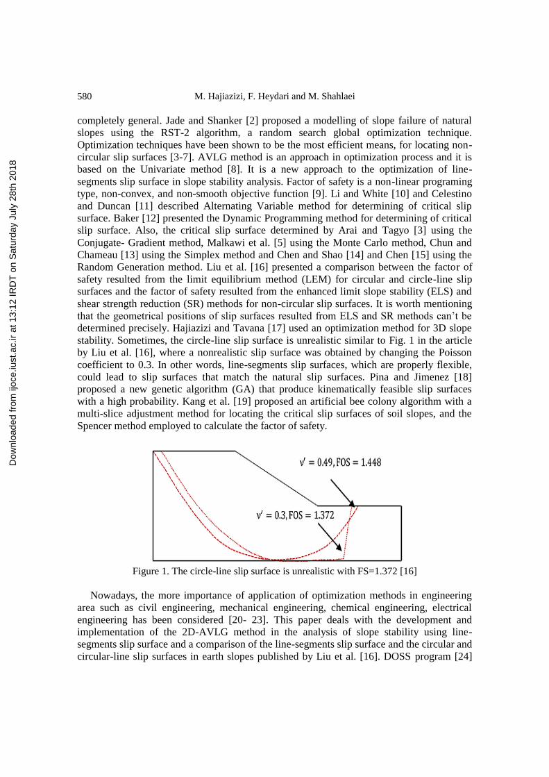
stability. Sometimes, the circle-line slip surface is unrealistic similar to Fig. 1 in the article
by Liu et al. [16], where a nonrealistic slip surface was obtained by changing the Poisson
coefficient to 0.3. In other words, line-segments slip surfaces, which are properly flexible,
could lead to slip surfaces that match the natural slip surfaces. Pina and Jimenez [18]
proposed a new genetic algorithm (GA) that produce kinematically feasible slip surfaces
with a high probability. Kang et al. [19] proposed an artificial bee colony algorithm with a
multi-slice adjustment method for locating the critical slip surfaces of soil slopes, and the
Spencer method employed to calculate the factor of safety.
Figure 1. The circle-line slip surface is unrealistic with FS=1.372 [16]
Nowadays, the more importance of application of optimization methods in engineering
area such as civil engineering, mechanical engineering, chemical engineering, electrical
engineering has been considered [20- 23]. This paper deals with the development and
implementation of the 2D-AVLG method in the analysis of slope stability using line-
segments slip surface and a comparison of the line-segments slip surface and the circular and
circular-line slip surfaces in earth slopes published by Liu et al. [16]. DOSS program [24]
Dow
nloa
ded
from
ijoc
e.iu
st.a
c.ir
at 1
3:12
IRD
T o
n S
atur
day
July
28t
h 20
18
Page 3
LINE-SEGMENTS CRITICAL SLIP SURFACE IN EARTH SLOPES USING AN … 581
was written by authors for obtaining the circular critical slip surfaces and line-segments
critical slip surface that is more consistent with the actual slip surface in the nature. Finally,
the results of this program will be compared with those obtained from LEM and two finite
element methods (ELSM and SRM) published by Liu et al. [16].
2. 2D ALTERNATING VARIABLE LOCAL GRADIENT METHOD
The AVLG method is based on the theory of the Univariate method. The Univariate method
is described as follows [8]:
1. Select an arbitrary starting point 𝑿𝑖 and set 𝑖 = 1
2. Find the search direction 𝑺𝑖
𝑺𝑖𝑇 =
{
(1,0,0,… ,0) for 𝑖 = 1, 𝑛 + 1, 2𝑛 + 1,…
(0,1,0,… ,0) for 𝑖 = 2, 𝑛 + 2, 2𝑛 + 2,…(0,0,1,… ,0) for 𝑖 = 3, 𝑛 + 3, 2𝑛 + 3,…
.
.
..
(0,0,0,… ,1) for 𝑖 = 𝑛 , 2𝑛 , 3𝑛 , …
(1)
3. Find the optimal step length λi∗ that
𝑓(𝑿𝑖 ± 𝜆𝑖∗𝑺𝑖) = 𝑚𝑖𝑛(𝑿𝑖 ± 𝜆𝑖𝑺𝑖) (2)
4. Consider Xi+1 = Xi ± λi∗Si , depending on the direction for decreasing the value f, and
fi+1=f(Xi+1)
5. Consider the new value of i = i + 1 and repeat from step 2.
For finding the most critical line-segments slip surface the AVLG method in 2D can be
described as follows:
1. Set i=1
2. Finding the circular critical slip surface and taking it as the initial slip surface.
3. Selecting the suitable nodes on the circular critical slip surface and connecting them to
each other. Zi denotes the coordinates of the initial nodes.
𝒁𝑖 = (𝑥1, 𝑦1, 𝑥2, 𝑦2, … , 𝑥𝑛, 𝑦𝑛) (3)
4. The best location for the first node on the slope boundary.
The new coordinates of slip surface are:
𝒁𝒊∗ = (𝑥1
∗, 𝑦1∗, 𝑥2, 𝑦2, … , 𝑥𝑛, 𝑦𝑛) (4)
5. The best location for the next node while also keeping the other nodes fixed results in a
lower factor of safety. The best location for each internal node is obtained by its moving
in the negative direction of the local gradient vector. The equation for the negative
direction of the local gradient vector is:
Dow
nloa
ded
from
ijoc
e.iu
st.a
c.ir
at 1
3:12
IRD
T o
n S
atur
day
July
28t
h 20
18
Page 4
M. Hajiazizi, F. Heydari and M. Shahlaei
582
𝑺𝑘 = −𝑮𝑘 = −{𝜕𝐹𝑠
𝜕𝑥𝑘,𝜕𝐹𝑠
𝜕𝑦𝑘}𝑇
(5)
where, the new coordinates of the slip surface are:
𝒁𝑖∗ = (𝑥1
∗, 𝑦1∗, 𝑥2
∗, 𝑦2∗, 𝑥3, 𝑦3, … , 𝑥𝑛, 𝑦𝑛) (6)
6. Find the best location for the subsequent internal node while other nodes remain fixed.
This process is iterated for the rest of the internal nodes. The new coordinates of the slip
surface are as follows:
𝒁𝑖∗ = (𝑥1
∗, 𝑦1∗, 𝑥2
∗, 𝑦2∗, … , 𝑥𝑘
∗ , 𝑦𝑘∗ , … , 𝑥𝑛, 𝑦𝑛) (7)
7. Finding the best location for the last node which the first optimization cycle is
terminated. The new coordinates of the slip surface are:
𝒁𝑖+1∗ = (𝑥1
∗, 𝑦1∗, 𝑥2
∗, 𝑦2∗, … , 𝑥𝑛−1
∗ , 𝑦𝑛−1∗ , 𝑥𝑛
∗ , 𝑦𝑛∗) (8)
8. Set i=i+1
9. Steps 4 to 7 are repeated for several cycles and new coordinates are obtained until the
difference between the safety factors of the last two cycles is less than ε=1×10⁻⁵. Or
|𝐹𝑆(𝐙i+1∗ ) − 𝐹𝑆(𝐙i
∗)| < ε (9)
FS (Z*i+1) = for the last optimization cycle,
FS (Z*i) = for the penultimate optimization cycle.
FS (Z*i+1) is taken as the most critical slip surface.
3. SLOPE STABILITY ANALYSIS METHODS
The slope stability analysis is a statically indeterminate problem, and there are different
methods of analysis available to the designer. Slope stability analysis can be carried out by
using the limit equilibrium method (LEM), the limit analysis method (LAM) and numerical
methods (NMs). The factor of safety for slope stability analysis is usually defined from the
shear strength to the shear stress ratio at a given failure. There are several ways in
formulating the factor of safety.
3.1 Limit equilibrium method
The limit equilibrium method is an approach in slope stability analysis. This method,
statically is an indeterminate problem, and assumptions on the inter-slice shear forces are
required to change to statically a determinate problem. Based on the assumptions there are
more than ten methods developed for slope stability analysis, such as the Fellenius method,
the Bishop simplified, Spencer, and Morgenstern-Price methods [7].
Dow
nloa
ded
from
ijoc
e.iu
st.a
c.ir
at 1
3:12
IRD
T o
n S
atur
day
July
28t
h 20
18
Page 5
LINE-SEGMENTS CRITICAL SLIP SURFACE IN EARTH SLOPES USING AN … 583
In the conventional limiting equilibrium method, the shear stress 𝜏𝑚 which can be
mobilized along the failure surface is given by:
𝜏𝑚 = 𝜏𝑓 𝐹𝑆⁄ (10)
where FS is the factor of safety, 𝜏𝑓 is shear strength as follows,
𝜏𝑓 = 𝑐′ + 𝜎�́� tan �́� (11)
where 𝑐′ is the effective cohesion, 𝜎′𝑛 is the effective normal stress, 𝜑′ is the angle of
effective internal friction.
In briefly the LEM formulation is written as follows:
𝐹𝑆 =𝑠ℎ𝑒𝑎𝑟 𝑠𝑡𝑟𝑒𝑔𝑡ℎ 𝑜𝑛 𝑎 𝑔𝑖𝑣𝑒𝑛 𝑠𝑙𝑖𝑝 𝑠𝑢𝑟𝑓𝑎𝑐𝑒
𝑠ℎ𝑒𝑎𝑟 𝑠𝑡𝑟𝑒𝑠𝑠 𝑜𝑛 𝑎 𝑔𝑖𝑣𝑒𝑛 𝑠𝑙𝑖𝑝 𝑠𝑢𝑟𝑓𝑎𝑐𝑒 (12)
Eq. (12) can also be written as follows:
𝜏𝑖 =𝜏𝑓𝑖𝐹𝑆
=𝑐′ + 𝜎′𝑖 tan �́�
𝐹𝑆=𝑐′
𝐹𝑆+ 𝜎′𝑖
tan𝜑′
𝐹𝑆 (13)
Conventionally, the critical slip surface for a given slope is estimated by comparing
safety factors of several trial slip surfaces. Among all trial slip surfaces, the slip surface that
has the lowest factor of safety is selected as the critical failure surface. Several optimization
approaches by using LEM have been employed to automate the search for the critical failure
surface [3-6].
3.1.1 The objective function for optimization
The objective function of the factor of safety is nonlinear non-smooth. Then the search for
global critical slip surface of soil slope is difficult as the objective function of the safety
factor. The objective function for optimization is,
n
i ii
iiiiiin
i
ii
xxf1
2
1
0
FS
tan tan 1
sec tan ) u - W( C
tan W
1 FS
(14)
Or
iGf /F FS i0 (15)
where
Dow
nloa
ded
from
ijoc
e.iu
st.a
c.ir
at 1
3:12
IRD
T o
n S
atur
day
July
28t
h 20
18
Page 6
M. Hajiazizi, F. Heydari and M. Shahlaei
584
)tan1(tantan
1
tan)( F 2
i iii
iiii
FS
xuwxC
(16)
iiw tanG i
(17)
2
)( 111
iiiiiii xxyfyfw
(18)
iiiii xxyy 11 /tan
(20)
This optimization problem cannot be solved directly, because the right-hand side of Eq.
14 includes FS. Here the following numerical graphical method is employed. In the
numerical graphical solution scheme, the optimization problem is solved provisionally for
an assumed value of FS in the right-hand side Eq. 14 and a plot is made in a way shown in
Fig. 2. Repetition of this operation yields curves, which specify the relation between two FS.
The point of intersection between the curve and the straight line with unit gradient such as in
Fig. 2 gives a solution of this problem.
Figure 2. Numerical graphical solution scheme
The gradient of the objective function FS on xi and yi are calculated as,
n
j
j
n
j
n
j
n
j
n
j
ijjjij
i
xxx 1
2
1 1 1 1
)G/()/G(F - G) /F( FS
(20)
and
n
j
j
n
j
n
j
n
j
n
j
ijjjij
i
yyy 1
2
1 1 1 1
)G/()/G(F - G) /F( FS
(21)
where,
Dow
nloa
ded
from
ijoc
e.iu
st.a
c.ir
at 1
3:12
IRD
T o
n S
atur
day
July
28t
h 20
18
Page 7
LINE-SEGMENTS CRITICAL SLIP SURFACE IN EARTH SLOPES USING AN … 585
n
j
iiiiij xxx1
1 /F /F /F (22)
n
j
iiiiij yyy1
1 /F /F /F
(23)
n
j
iiiiij xxx1
1 /G /G /G
(24)
n
j
iiiiij yyy1
1 /G /G /G
(25)
i
i
iiiii
i
i
xx
y
2tan FS)
tan WC()tanFS(1 tan 0.5[-
Fi
2
] tan )tanFS(1) tan W
C() tan tan (FS 2
ii
i
iiiii
x
(26)
2) tan tan FS/( ii
(26)
1
1
11i1
2
11 2tan FS)
tan WC()tanFS(1 tan 0.5[-
Fi
i
iiiii
i
i
xx
y
] tan )tanFS(1) tan W
C() tan tan (FS 1
2
1
111 ii
i
iiiii
x
2
1 ) tan tan FS/( ii
(27)
0 /G ii x
(28)
)2( 0.5 /G 1 iiiii ffyy
(29)
0 /G 1 ii x
(30)
)2( 0.5 /G 11 iiiii yffy
(31)
The partial derivatives of a function FS, with respect to each of the 2n variables are
collectively called the gradient of the function and is denoted by FS,
n
n
n
y
x
y
x
FS/
FS/
FS/
FS/
FS
1
1
12 (32)
3.2 Shear strength reduction method (SRM)
In the SRM, the gravity load vector for a material with unit weight 𝛾𝑠 is determined from Eq.
(33) as follows [25]:
Dow
nloa
ded
from
ijoc
e.iu
st.a
c.ir
at 1
3:12
IRD
T o
n S
atur
day
July
28t
h 20
18
Page 8
M. Hajiazizi, F. Heydari and M. Shahlaei
586
{𝑓} = 𝛾𝑠∫[𝑁]𝑇𝑑𝑣 (33)
where {f} is the equivalent body force vector and [𝑁] is the shape factor matrix. The
material parameters 𝑐′ and 𝜑′ are reduced according to
𝑐′𝑓 =𝑐′
𝐹𝑆; 𝜑′𝑓 = 𝑎𝑟𝑐 tan{tan(𝜑′ 𝐹𝑆⁄ )} (34)
The factor of safety FS keeps on changing until the ultimate state of the system is
attained, and the corresponding factor of safety will be the factor of safety of the slope [25].
The location of the critical failure surface is usually determined from the contour of the
maximum shear strain or the maximum shear strain rate. SRM can give, movements and
pore pressures which are not possible with the LEM. However, the SRM unable to locate the
slip surface, exactly.
3.3 Enhanced limit slope stability (ELS) method
In the ELS method, the FS can be obtained as:
𝐹𝑆 =∑ 𝜏𝑓𝑖∆𝐿𝑖𝑛𝑖=1
∑ 𝜏𝑖∆𝐿𝑖𝑛𝑖=1
=∫ 𝜏𝑓𝑑𝑙
∫ 𝜏𝑑𝑙 (35)
where n=the number of discrete segments along L, ∆Li=the length of segment i. The
primary task of the ELS method is to locate the critical slip surface using mathematical
optimization [16].
4. EXAMPLES
To investigate the differences and compare the results of the AVLG method (line-segments
slip surface), LEM, SRM and ELSM (circular and line-circular slip surface), four examples
were selected from [16]. These examples have been widely used in the engineering
literature. In this article, the values of factor of safety and slip surfaces were calculated and
compared using the four aforementioned methods.
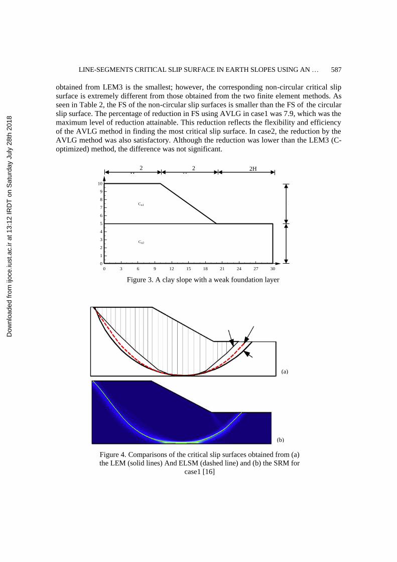
4.1 Example 1
The inclined surface studied in this example is depicted in Fig. 3. The embankment height is
equal to 5m and 𝐶𝑢1/𝛾𝐻 = 0.25. Table 1 shows the soil characteristics for two layers in Fig.
3. Fig. 4 compares the critical slip surfaces resulted from the limit equilibrium, the strength
reduction, and ELS methods. This figure was prepared by [16]. Fig. 5 shows the circular and
line-segment critical slip surfaces resulted from the AVLG method for case1 and case2. [16]
indicated that the FS resulted from ELS method was close to the FS resulted from SRM. In
Table 2, the FS obtained from LEM1 is larger than those obtained from the two finite
element methods, which could be explained by the assumed circular arc slip surface. The FS
Dow
nloa
ded
from
ijoc
e.iu
st.a
c.ir
at 1
3:12
IRD
T o
n S
atur
day
July
28t
h 20
18
Page 9
LINE-SEGMENTS CRITICAL SLIP SURFACE IN EARTH SLOPES USING AN … 587
obtained from LEM3 is the smallest; however, the corresponding non-circular critical slip
surface is extremely different from those obtained from the two finite element methods. As
seen in Table 2, the FS of the non-circular slip surfaces is smaller than the FS of the circular
slip surface. The percentage of reduction in FS using AVLG in case1 was 7.9, which was the
maximum level of reduction attainable. This reduction reflects the flexibility and efficiency
of the AVLG method in finding the most critical slip surface. In case2, the reduction by the
AVLG method was also satisfactory. Although the reduction was lower than the LEM3 (C-
optimized) method, the difference was not significant.
(b)
Figure 4. Comparisons of the critical slip surfaces obtained from (a)
the LEM (solid lines) And ELSM (dashed line) and (b) the SRM for
case1 [16]
(a)
A
B C
0 3 6 9 12 15 18 21 24 27 30
0
1
2
3
4
5
6
7
8
9
10
Cu1
Cu2
Figure 3. A clay slope with a weak foundation layer
H
H
2H 2
H
2
H
Dow
nloa
ded
from
ijoc
e.iu
st.a
c.ir
at 1
3:12
IRD
T o
n S
atur
day
July
28t
h 20
18
Page 10
M. Hajiazizi, F. Heydari and M. Shahlaei
588
Table 1: Geotechnical parameters for example 1
Case 𝛾(𝑘𝑁 𝑚3)⁄ 𝑐𝑢2 𝑐𝑢1 (−)⁄ 𝐸(𝑘𝑁 𝑚2)⁄ 𝜗(−)
1 20.0 1.0 105 0.49
2 20.0 0.8 105 0.49
Table 2: Factors of safety for example1
Method Case1
FS difference
with Circular slip
surface Case2
FS difference
with Circular
slip surface
LEM1(A-circular) [16] 1.474 1.235
LEM2(B-fully specified) [16] 1.455 1.3 1.202 2.7
LEM3(C-optimized) [16] 1.362 7.6 1.120 9.3
SRM(Coarse mesh) [16] 1.460 0.95 1.210 2
SRM(fine mesh) [16] 1.451 1.6 1.215 1.6
ELSM [16] 1.448 1.7 1.211 1.9
AVLG(LEM-critical circular slip
surface)[this study] 1.440 1.230
AVLG(critical line-segments slip
surface)[this study] 1.326 7.9 1.116 9.2
Figure 5. Comparison between initial and optimization slip surfaces
with DOSS software (a) case1, (b) case2 (this study)
0 3 6 9 12 15 18 21 24 27 30
0
1
2
3
4
5
6
7
8
9
10Circular Critical Slip Surface
Non-Circular Critical Slip Surface
0 3 6 9 12 15 18 21 24 27 30
0
1
2
3
4
5
6
7
8
9
10Circular Slip Surface
Non-Circular Slip Surface
(
a)
(
b)
Dow
nloa
ded
from
ijoc
e.iu
st.a
c.ir
at 1
3:12
IRD
T o
n S
atur
day
July
28t
h 20
18
Page 11
LINE-SEGMENTS CRITICAL SLIP SURFACE IN EARTH SLOPES USING AN … 589
4.2 Example 2
In this example, a homogeneous soil slope with a slope height equal to H=5 m, slope
angle equal to 25.67° and 𝑐 ́ /𝛾𝐻 = 0.05 is considered (Fig. 6). The soil characteristics
show in Table 3. The critical slip surfaces from the two finite element methods and the
limit equilibrium method (Fig. 7) and AVLG method (Fig. 8) are in good agreement. As
seen in Table 4, the non-circular slip surfaces of SRM and ELS method resulted in larger
factors of safety as compared to the circular slip surfaces obtained by [16]. The values of
critical line-segments and circular FS resulted from the AVLG method were 1.166 and
1.35, respectively. The 13.6% reduction in FS values reflected the effectiveness of the
line-segment slip surface to find smaller factors of safety.
0 2 4 6 8 10 12 14 16
0
0.5
1
1.5
2
2.5
3
3.5
4
4.5
5
Figure 6. A homogeneous slope with a
slope angle of 25.67° (2: 1), 𝑐 𝛾𝐻⁄ = 0.05
H
2
H
1.
2H
Dow
nloa
ded
from
ijoc
e.iu
st.a
c.ir
at 1
3:12
IRD
T o
n S
atur
day
July
28t
h 20
18
Page 12
M. Hajiazizi, F. Heydari and M. Shahlaei
590
Table 3: Geotechnical parameters for example 2
𝛾(𝑘𝑁 𝑚3)⁄ 𝜑 (°) 𝐸(𝑘𝑁 𝑚2)⁄ 𝜗(−)
20.0 20.0 105 0.40
Table 4: Summary of factors of safety for example 2
Method Safety FS difference with
Figure 8. Comparison of initial and optimization slip
surfaces with DOSS software for example 2 (this study)
0 2 4 6 8 10 12 14 16
0
0.5
1
1.5
2
2.5
3
3.5
4
4.5
5
Non-Circular Slip Surface
Circular Slip Surface
Figure 7. Comparisons of the critical slip
surfaces obtained from (a) the LEM (solid line)
and ELSM (dashed line) (b) the SRM [16]
(b
)
(a
)
Dow
nloa
ded
from
ijoc
e.iu
st.a
c.ir
at 1
3:12
IRD
T o
n S
atur
day
July
28t
h 20
18
Page 13
LINE-SEGMENTS CRITICAL SLIP SURFACE IN EARTH SLOPES USING AN … 591
Factor Circular slip surface
LEM (Bishop/Geo-slope, Circular) [16] 1.376
SRM [16] 1.387 -0.8
ELSM [16] 1.384 -0.6
AVLG(LEM-critical circular slip surface) [this study] 1.350
AVLG(critical line-segments slip surface) [this study] 1.166 +13.6
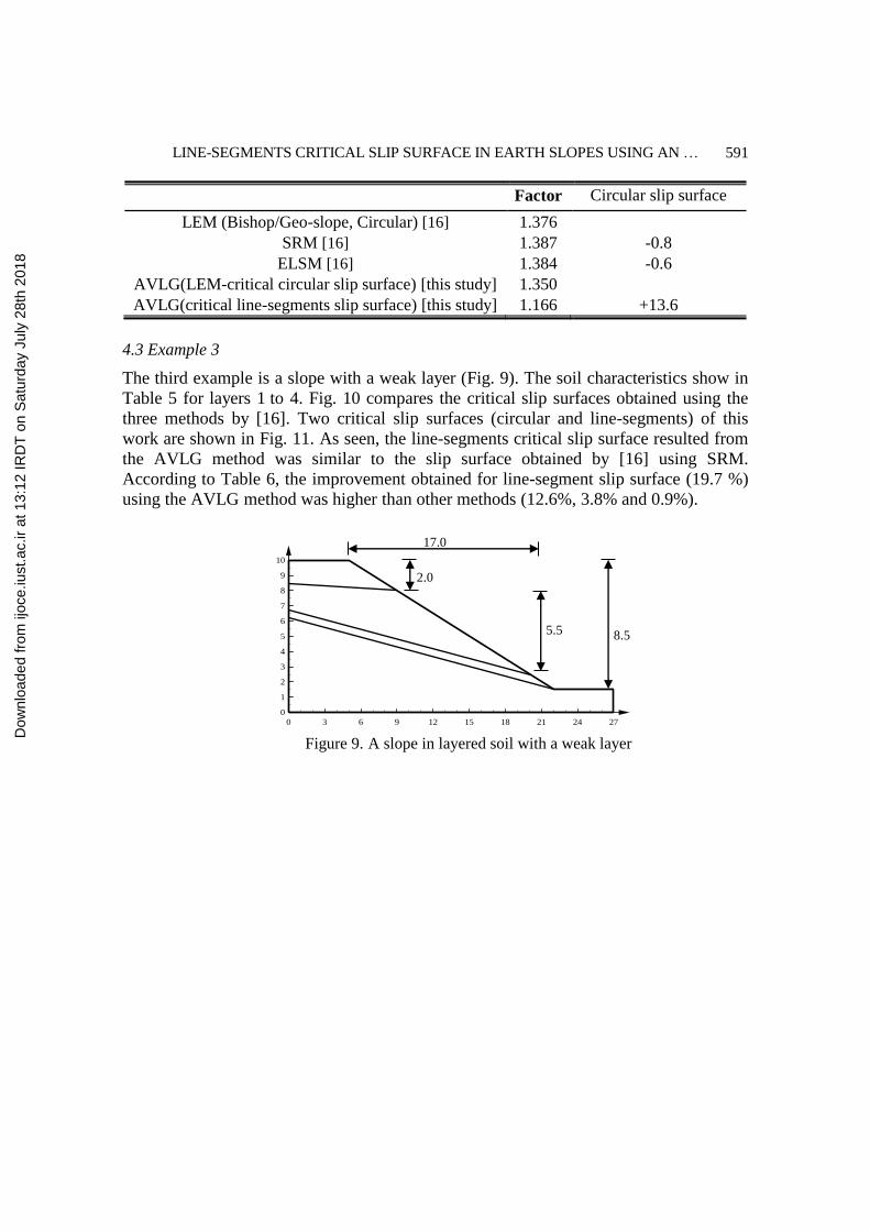
4.3 Example 3
The third example is a slope with a weak layer (Fig. 9). The soil characteristics show in
Table 5 for layers 1 to 4. Fig. 10 compares the critical slip surfaces obtained using the
three methods by [16]. Two critical slip surfaces (circular and line-segments) of this
work are shown in Fig. 11. As seen, the line-segments critical slip surface resulted from
the AVLG method was similar to the slip surface obtained by [16] using SRM.
According to Table 6, the improvement obtained for line-segment slip surface (19.7 %)
using the AVLG method was higher than other methods (12.6%, 3.8% and 0.9%).
Figure 9. A slope in layered soil with a weak layer
0 3 6 9 12 15 18 21 24 27
0
1
2
3
4
5
6
7
8
9
10
8.5
0
5.5
5
2.0
0
17.0
0
Dow
nloa
ded
from
ijoc
e.iu
st.a
c.ir
at 1
3:12
IRD
T o
n S
atur
day
July
28t
h 20
18
Page 14
M. Hajiazizi, F. Heydari and M. Shahlaei
592
Table 5: Geotechnical parameters for example 3
Layer 𝛾(𝑘𝑁 𝑚3)⁄ 𝑐 (𝑘𝑃𝑎) 𝜑 (°) 𝐸(𝑘𝑁 𝑚2)⁄ 𝜗(−)
1 18.62 15.0 20.0 105 0.35
2 18.62 17.0 21.0 105 0.35
3 18.62 5.0 10.0 105 0.35
4 18.62 35.0 28.0 105 0.35
Table 6: Summary of factors of safety for example 3
Method Safety
Factor
FS difference with
Circular slip surface
LEM1 (M-P, Non-circular) [7] 1.240 12.6
0 3 6 9 12 15 18 21 24 27
0
1
2
3
4
5
6
7
8
9
10
Circular Slip Surface
Non-Circular Slip Surface
Figure 11. Comparison between initial and optimization slip
surfaces using AVLG method for example 3 (this study)
Figure 10. Comparisons of the critical slip surfaces obtained
from (a) the LEM (solid line and dotted line) and ELSM
(dashed line) and (b) the SRM [16]
(a)
(b)
Dow
nloa
ded
from
ijoc
e.iu
st.a
c.ir
at 1
3:12
IRD
T o
n S
atur
day
July
28t
h 20
18
Page 15
LINE-SEGMENTS CRITICAL SLIP SURFACE IN EARTH SLOPES USING AN … 593
LEM2 (Spencer, Non-circular) [7] 1.101
SRM [16] 1.143 3.8
ELSM [16] 1.111 0.9
AVLG(LEM-critical circular slip surface)[this study] 1.424
AVLG(critical line-segments slip surface)[this study] 1.143 19.7
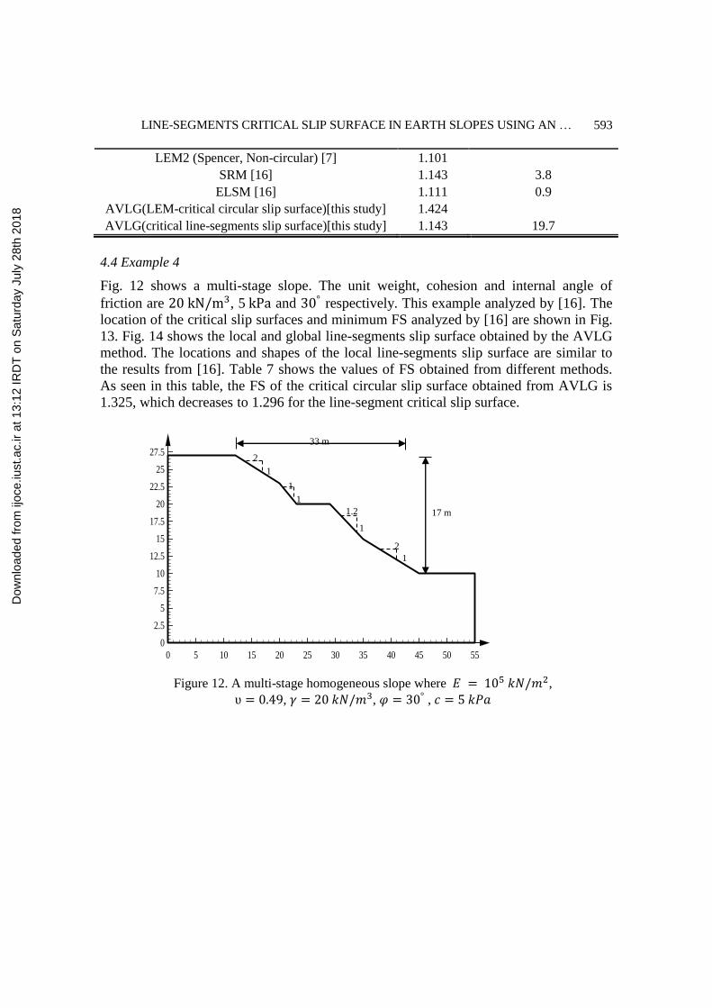
4.4 Example 4
Fig. 12 shows a multi-stage slope. The unit weight, cohesion and internal angle of
friction are 20 kN/m3, 5 kPa and 30° respectively. This example analyzed by [16]. The
location of the critical slip surfaces and minimum FS analyzed by [16] are shown in Fig.
13. Fig. 14 shows the local and global line-segments slip surface obtained by the AVLG
method. The locations and shapes of the local line-segments slip surface are similar to
the results from [16]. Table 7 shows the values of FS obtained from different methods.
As seen in this table, the FS of the critical circular slip surface obtained from AVLG is
1.325, which decreases to 1.296 for the line-segment critical slip surface.
2
1.2
2
0 5 10 15 20 25 30 35 40 45 50 55
0
2.5
5
7.5
10
12.5
15
17.5
20
22.5
25
27.5
1
1
1
1
1
Figure 12. A multi-stage homogeneous slope where 𝐸 = 105 𝑘𝑁/𝑚2,
ʋ = 0.49, 𝛾 = 20 𝑘𝑁/𝑚3, 𝜑 = 30° , 𝑐 = 5 𝑘𝑃𝑎
17 m
33 m
Dow
nloa
ded
from
ijoc
e.iu
st.a
c.ir
at 1
3:12
IRD
T o
n S
atur
day
July
28t
h 20
18
Page 16
M. Hajiazizi, F. Heydari and M. Shahlaei
594
Figure 14. Line-segments critical slip surface and FS
obtained from the AVLG method (this study)
0 5 10 15 20 25 30 35 40 45 50 55
0
2.5
5
7.5
10
12.5
15
17.5
20
22.5
25
27.5
FOS=1.427
FOS=1.331
FOS=1.310
FOS=1.296
FOS=1.360
Figure 13. Comparisons of the slip surface: (a) critical slip
surfaces obtained from the SRM and (b) critical failure surface
from the ELSM [16]
(a)
(b)
Dow
nloa
ded
from
ijoc
e.iu
st.a
c.ir
at 1
3:12
IRD
T o
n S
atur
day
July
28t
h 20
18
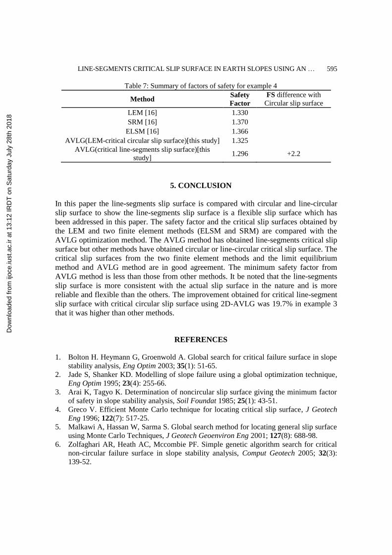
Page 17
LINE-SEGMENTS CRITICAL SLIP SURFACE IN EARTH SLOPES USING AN … 595
Table 7: Summary of factors of safety for example 4
Method Safety
Factor
FS difference with
Circular slip surface
LEM [16] 1.330
SRM [16] 1.370
ELSM [16] 1.366
AVLG(LEM-critical circular slip surface)[this study] 1.325
AVLG(critical line-segments slip surface)[this
study] 1.296 +2.2
5. CONCLUSION
In this paper the line-segments slip surface is compared with circular and line-circular
slip surface to show the line-segments slip surface is a flexible slip surface which has
been addressed in this paper. The safety factor and the critical slip surfaces obtained by
the LEM and two finite element methods (ELSM and SRM) are compared with the
AVLG optimization method. The AVLG method has obtained line-segments critical slip
surface but other methods have obtained circular or line-circular critical slip surface. The
critical slip surfaces from the two finite element methods and the limit equilibrium
method and AVLG method are in good agreement. The minimum safety factor from
AVLG method is less than those from other methods. It be noted that the line-segments
slip surface is more consistent with the actual slip surface in the nature and is more
reliable and flexible than the others. The improvement obtained for critical line-segment
slip surface with critical circular slip surface using 2D-AVLG was 19.7% in example 3
that it was higher than other methods.
REFERENCES
1. Bolton H. Heymann G, Groenwold A. Global search for critical failure surface in slope
stability analysis, Eng Optim 2003; 35(1): 51-65.
2. Jade S, Shanker KD. Modelling of slope failure using a global optimization technique,
Eng Optim 1995; 23(4): 255-66.
3. Arai K, Tagyo K. Determination of noncircular slip surface giving the minimum factor
of safety in slope stability analysis, Soil Foundat 1985; 25(1): 43-51.
4. Greco V. Efficient Monte Carlo technique for locating critical slip surface, J Geotech
Eng 1996; 122(7): 517-25.
5. Malkawi A, Hassan W, Sarma S. Global search method for locating general slip surface
using Monte Carlo Techniques, J Geotech Geoenviron Eng 2001; 127(8): 688-98.
6. Zolfaghari AR, Heath AC, Mccombie PF. Simple genetic algorithm search for critical
non-circular failure surface in slope stability analysis, Comput Geotech 2005; 32(3):
139-52.
Dow
nloa
ded
from
ijoc
e.iu
st.a
c.ir
at 1
3:12
IRD
T o
n S
atur
day
July
28t
h 20
18
Page 18
M. Hajiazizi, F. Heydari and M. Shahlaei
596
7. Cheng YM, Li L, Chi SC, Wei WB. Particle swarm optimization algorithm for the
location of the critical non-circular failure surface in two-dimensional slope stability
analysis, Comput Geotech 2007; 34(2): 92-103.
8. Rao SS. Optimization Theory and Applications, 2nd, Chapter 5, Wiley Eastern Limited,
1984.
9. Cheng YM. Locations of critical failure surface and some further studies on slope
stability analysis, Comput Geotech 2003; 30: 255-67.
10. Li KS, White W. Rapid evaluation of the critical slip surface in slope stability problems,
Int J Numer Analyt Method Geomech 1987; 11: 449-73.
11. Celestino, T.B. and Duncan, J.M. Simplified search for non-circular slip surfaces,
Proceedings of the 10th International Conference on Soil Mechanics and Foundation
Engineering 1981, International Society for Soil Mechanics and Foundation
Engineering, Stockholm, 3. A.A. Balkema, Rotterdam, Holland, pp. 391-394.
12. Baker R. Determination of the critical slip surface in slope stability computations, Int J
Numer Analyt Method Geomech 1980; 4(4): 333-59.
13. Chun RH, Chameau JL. Three-dimensional limit equilibrium analysis of slopes,
Geotech 1982; 32(1): 31-40.
14. Chen Z, Shao C. Evaluation of minimum factor of safety in slope stability analysis,
Canadian Geotech J 1983; 25(4): 735-48.
15. Chen Z. Random trials used in determining global minimum factors of safety of slopes,
Canadian Geotech J 1992; 29(2): 225-33.
16. Liu SY, Shao LT, Li HJ. Slope stability analysis using the limit equilibrium method and
two finite element methods, Comput Geotech 2015; 63: 291-8.
17. Hajiazizi M, Tavana H. Determining three-dimensional non-spherical critical slip
surface in earth slopes using an optimization method, Eng Geology 2013; 153: 114-24.
18. Piña RJ, Jimenez R. Genetic algorithm for slope stability analyses with concave slip
surfaces using custom operators, Eng Optim 2015; 47(4): 453-72.
19. Kang F, Li J, Ma Z. An artificial bee colony algorithm for locating the critical slip
surface in slope stability analysis, Eng Optim 2013, 45(2): 207-23.
20. García-Palacios J, Castro C, Samartín, A. Optimal design in elasticity: a systematic
adjoint approach to boundary cost functionals, Optim Eng 2015; 16(4): 811-29.
21. Herzog R, Riedel I. Sequentially optimal sensor placement in thermoelastic models for
real time applications, Optim Eng 2015; 16(4): 736-66.
22. Gheribi AE, Harvey JP, Bélisle E, Robelin C, Chartrand P, Pelton AD, Balel CW,
Digabe SL. Use of a biobjective direct search algorithm in the process design of
material science applications, Optim Eng 2016; 17(1): 1-19.
23. Diouane Y, Gratton S, Vasseur X, Vicente LN, Calandra H. A parallel evolution
strategy for an earth imaging problem in geophysics, Optim Eng 2016; 17(1): 1-24.
24. DOSS program, Software of Determination of Optimal Slip Surface, Razi University,
Iran, 2010.
25. Griffiths DV, Lane PA. Slope stability analysis by finite elements, Géotech 1999; 49(3):
387-403.
Dow
nloa
ded
from
ijoc
e.iu
st.a
c.ir
at 1
3:12
IRD
T o
n S
atur
day
July
28t
h 20
18


![Estimating Road Segments Using Natural Point ...segments”-contest [6] was organized with the task of averaging segments of GPS trajectories to predict road segments while including](https://static.documents.pub/doc/80x56/60cfe59c42219c07ae1490d1/estimating-road-segments-using-natural-point-segmentsa-contest-6-was-organized.jpg)


![1 Regularised non-uniform segments and efficient no-slip ...arXiv:2008.12339v1 [physics.flu-dyn] 27 Aug 2020 1 Regularised non-uniform segments and efficient no-slip elastohydrodynamics](https://static.documents.pub/doc/80x56/6149a8e812c9616cbc68e7b6/1-regularised-non-uniform-segments-and-eifcient-no-slip-arxiv200812339v1-.jpg)
