JOURNAL OF THE OPTICAL SOCIETY OF AMERICA

Line Spread Function and Cumulative Line Spread Function forSystems with Rotational Symmetry

RICHARD BARAXAT AND AG:NES HOUSTON

Optics Department, Research Division, Itek Corporation, Lexington, Massachusetts 02173(Received 11 December 1963)

The line spread function and the cumulative line spread function for a circular aperture having rotationallysymmetric aberrations are determined by integrals involving the transfer function of the system. Asymptoticexpansions of the line spread function and the cumulative line spread function are obtained from a knowledgeof the transfer function and its derivatives evaluated at zero spatial frequency. The moments of the transferfunction determine the behavior of the line spread function and the cumulative line spread function forsmall values of the argument. Typical numerical results are also presented.

1. INTRODUCTION

IN the present paper we consider the images formedby circular apertures for incohlerent line sources,

the circular apertures being allowed to possess sphericalaberration. In addition to studying the line spreadfunction we also consider the cumulative line spreadfunction. Although the point spread function and linespread function are related via a rather complicatedAbel integral equation, we have found it most useful toemploy the transfer function in deriving the propertiesof the line and cumulative line spread functions. Typicalnumerical results are also presented.

Let 1(v) be the rotationally symmetric point spreadfunction of a circular aperture where V2= vi+vj. Thedimensionless parameter v is given by the relation

v = (ir/XF)z,

where A is measured in microns, F is the f number ofthe system, and z is the lateral distance in microns fromthe center of the optical axis. The function obtained byintegrating 1(v) over an infinite line in the image planeis termed the line spread function. Clearly no generalityis lost by integrating over the v1, axis, consequently:

Equation (1.2) is a Volterra integral equation of thefirst kind if we consider the line spread function as theknown function and the point spread function as theunknown. To put (1.2) into the standard form of anAbel integral equation, we make the substitutions

and obtain

r° 1(aedae r t(atjdaT - `1 =: - I2o-_-- = 012 1 (

Finally upon letting

4j2] =/2131Q); rc[ra ]= aS2l(a),

we havej S2(a)da

S() =( O Co a)§

(1.4)

(1.5)

(1.6)

(1.7)

which is Abel's integral equation.4 The inversion of thisintegral equation is shown by Tricomi to be

SI(0) 1S2 (A)= +-

TQ wr

J Sl'(a)da

(-ad-) 1(1.8)

Tr(v) = I [(V A+V,) I]dv,. (1.1)

This equation can be brought into somewhat morefamiliar form by letting v itself become the independentvariable, then (1.2) reads

A= f (v)vdvTr(v,,) = 21-

J . (v2-a ~2)1.(1.2)

In the case of a perfect system in the Fraunhofer re-ceiving plane, (1.2) becomes

fX J 12 (v)v-ldv

r(V2 ) = 8 I v - ). (V (2-V,2) i

(1.3)

It is in this form that the line spread function wasstudied by Struve,' Andre,2 and Rayleigh.3

'IH. Struve, Ann. Physik 17, 1008 (1882).2 Ch. Andre, Ann. Ecole Normale Suppl. No. 5 (1876).' Lord Rayleigh, in "Wave Theory of Light," Scientific Papers

(Cambridge University Press, Cambridge, England, 1902), Vol. 3.

provided that the line spread function be differentiable(which it is).

We now go back to the original variables

S = (1) 1 dr('-1)2,(3- fl dubs

=- (v./2)Tr(v)- (vA4/2)r'(vl) (1.9)

upon employing (1.4). The term involving S,(0)vanishes, leaving

I -l E7(V)+v-r (v)]zlduVz"3t Vz) =- __ -

Hr i 0 3 ( vy 2

-r-2) i

: I -T(v)+V77(V)]dV= ,

(1.10)

(1.11)

IF. G. Tricomi, Integral Equations (Interscience PublishersInc., New York, 1958), p. 39,

768

VOLUME 54, NUMBER 6 JUNE 1964

V2=a-1; V, 2 = 0-1,

LINE SPREAD FUNCTION

(1.12)

where we have let co= 2 cosx. This integral can be ex-pressed as a zero-order Struve functions

Finally we interchange the two variables for the finalanswer

1 C00

7rV2 J

EVX-r(vx2)+vX27(V)]dvx

(VX 2 - V2) j-(1.13)

which yields the point spread function in terms of theline spread function. Compare (1.13) with the formuladerived in Jones.5

We circumvent the necessity of dealing with (1.2) or(1.13) by dealing with the transfer function of thesystem. The transfer function is the two-dimensionalFourier transform of 1(v) which by reason of rotationalsymmetry becomes the Hankel transform

T(co) = t(v)Jo(vco)vdv,

also

T(c)= j r(vx)eivxwdvx= 21 r(v7 ) cosvxwdvx.

By inversion (1.15) becomes

2

Tr(v,) = N T(co) coscovxdc.

(1.14)

J 2r/2

0~l sin(2vx cosx)dx=-H,(2vx),2

consequently J2 , Ho(2vx)Tjl(x)= Zcos

1 - cosvvwdw =7rJ0 2 (2ho)

Upon making the substitution Cl= 2 cosx inwe have

/2

r2(Vx) = 21 cos(2vx cosx) cosx sin2xdx

1 r/1 2 cos(2vx cosx) cosxdx

2 / c1 rT/2

--T cos(2vx cosx) cos3xdx.2

(2.4)

(2.5)

(2.6)

(1.15) These integrals can be evaluated in terms of theLommel-Weber functions6 En.(z), in fact

(1.16)

Remember that T(o) 0 for w> 2 and N is a constantsuch that T(0) = 1. Consequently a knowledge of thetransfer function enables one to compute the line spreadfunction.

2. LINE SPREAD FUNCTION

We first derive the line spread function of a perfectsystem directly from the Fourier cosine transform.Recall that the transfer function of a perfect system is

T(ct)=- cos-l---0 ) 2 (2.1)

so that the line spread function reads

7r C2 CO 2/ @2\-T( 2,r =v cos-_ cosvdcod- -(1 V cosvwcodo,2 J6 2 2\ 4)

2 nor / 1r

E (2vx)= - sin- | cos(2vx cosx) cosnxdx,wr 2 ie

where n is a positive integer. Consequently

,,,(v) = (7r/4)[EI(2vx)+ E3(2vx)]

(2.7)

= 7r[E,(2v.)/(2v,)], (2.8)

where we have employed a reduction formula listed inWatson. Thus T(vS) reads

(v.)= [2/(2v.)][H,(2v7) - E2(2v,)]= [-2/(2v.)][Eo(2v,)+ E2(2v,)]. (2.9)

Since E2(z) is now a tabulated function, 7 we can considereither expression as the final formula. To put (2.9) intothe more usual form we employ the reduction formulagiven in Watson 6

Eo(2v,)+ E2 (2vz) = [2/(2v,)][E2 (2v7 ))- (2/r)]= -[H,(2v.)/vj,(2.10)

where HI is the Struve function of order unity. Finally (! !)

Integrate i-i(v,) by parts

1 (D2 1r1(v,)=-sinvZw cos-1- + _

V, 2 0 2vZ

== r(v,)- (r2V,)

2 sinvzwdwo

Jo(4&-2)1

1 T/ 2sin(2v, cosx)dx,

I R. C. Jones, J. Opt. Soc. Am. 48, 934 (1958).

(2.2) (2.11)

which is the usual expression for the line spread function.'

6 G. N. Watson, A Treatise on Bessel Functions (CambridgeUniversity Press, Cambridge, England, 1944).

7 G. D. Bernard and A. Ishimaru, Tables of the Anger andLommel Weber Functions (University of Washington Press, Seattle,1962).

(2 3) 8 One must be very careful in reading the literature because(2.11) masquerades in many forms due to various definitions of theStruve functions. We have employed the now standard notationof Watson.

769June 1964

t(Vx) = - I - EVT(V)+V2T'(V)]dv

7rvx2 . (V 2- VX 2) ��

,r(v,,) = 4EHI(2v�)/(2vj)1],

R. BARAKAT AND A. HOUSTON

TABLE I. Normalized line spread function r(v,,) of aberration-free system for various amounts of defocusing.

v 1Y 2 =0 IV2=0.2 W 2 =0.4 W2 =0.6 W 2 =0.8 W2 = 1.0 W 2 = 1.2

0 1.0 0.90831 0.68224 0.43289 0.25627 0.17863 0.162560.5 0.93520 0.85198 0.64633 0.41824 0.25456 0.17990 0.161601.0 0.76193 0.70165 0.55125 0.38046 0.25135 0.18421 0.159471.5 0.53410 0.50473 0.42863 0.33440 0.25067 0.19228 0.157772.0 0.31505 0.31644 0.31400 0.29505 0.25486 0.20332 0.157682.5 0.15228 0.17726 0.23120 0.29644 0.26163 0.21413 0.158993.0 0.06261 0.10027 0.18463 0.25412 0.26459 0.22018 0.160443.5 0.03331 0.07283 0.16237 0.23911 0.25696 0.21805 0.160914.0 0.03592 0.06958 0.14677 0.21544 0.23603 0.20775 0.160524.5 0.04352 0.06793 0.12556 0.18111 0.20529 0.19287 0.160525.0 0.04201 0.05759 0.09698 0.14180 0.17253 0.17845 0.162065.5 0.03137 0.04066 0.06756 0.10666 0.14538 0.16780 0.164726.0 0.01911 0.02497 0.04533 0.08229 0.12715 0.16055 0.166166.5 0.01196 0.01643 0.03391 0.06928 0.11570 0.15328 0.163367.0 0.01128 0.01524 0.03085 0.06291 0.10587 0.14220 0.154627.5 0.01370 0.01719 0.03042 0.05708 0.09333 0.12598 0.140938.0 0.01492 0.01771 0.02792 0.04835 0.07736 0.10671 0.12554

For small valuesapproximation'

of vZ, we have the series however T'(0) =- 2/7r for all systems irrespective of theamount of aberration. Consequently

,r(v) = (8/37r)-(32v,1/45r)+

while for large v,

Tr(v) > (2/7rvx2) +*-.

The asymptotic behavior of the line spread fucan be computed from a knowledge of the behathe transfer function at zero spatial frequency. Nlarge v, we have9

/W2 T'(0) T(3)(0)| T(cw) cosvt.wdcwy-' - + +0 v-)

vx2 Vj4

TABLE II. Values of transfer function of aberration-free systemfor various amounts of defocusing W2 in wavelength units.

1W2 =0.2 W2 =0.4 W2 =0.6 IV2 =0.8 W2 = 1.0 IV2 = 1.2

0 1.0 1.0 1.0 1.0 1.0 1.00.1 0.92975 0.91008 0.87793 0.83419 0.78008 0.717110.2 0.85100 0.78756 0.68887 0.56463 0.42662 0.287380.3 0.76956 0.65704 0.49419 0.31159 0.14110 0.008550.4 0.68957 0.53483 0.32922 0.13021 -0.01411 -0.082010.5 0.61373 0.42950 0.20605 0.02374 -0.06831 -0.070170.6 0.54353 0.34393 0.12248 0.02769 -0.06951 -0.032860.7 0.47957 0.27741 0.07029 0.04624 -0.05331 -0.003820.8 0.42175 0.33745 0.04046 0.04870 -0.03688 0.011330.9 0.36958 0.19088 0.02558 0.04463 -0.02571 0.016531.0 0.32228 0.16449 0.02038 0.03853 -0.02006 0.016151.1 0.27898 0.14535 0.02141 0.03181 -0.01847 0.012591.2 0.23878 0.13082 0.02642 0.02425 -0.01903 0.006791.3 0.20090 0.11855 0.03366 0.01503 -0.01950 -0.000661.4 0.16473 0.10643 0.04134 0.00355 -0.01730 -0.008081.5 0.12991 0.09266 0.04722 0.00963 -0.01014 -0.011861.6 0.09649 0.07599 0.04861 0.02186 0.00203 -0.007841.7 0.06497 0.05605 0.04310 0.02850 0.01472 0.003821.8 0.03651 0.03398 0.03003 0.02505 0.01949 0.013841,9 0,01323 0.01297 0.01255 0.01198 0.01126 0.010432.0 0 0 0 0 0 0

9 H. F. Willis, Phil. Mag. 39, 455 (1948).

(2.12) Tr(vx)- (217,vx2)+ ET(') (0)1vx4]+0(v -6), (2.15)

and T(vx) behaves as

,r(vx) 217rvxl (2.16)

for all systems provided vx be large enough. Comparewith (2.13).

For small values of vx expand the cosine term in apower series and integrate termwise, then

(2-14) r(vx)=f T(co)dwf-- T(w)c22dco

VX4 r2+-X T(o)o4dco+*-. (2.17)4!

The first term is nothing but the Struve criterion r(0)1I;in fact, the higher moments are also equal to thederivatives of -r(v) evaluated at the origin. In order toappreciate the usefulness of (2.17), we leave it to thereader to derive (2.12) directly from it.

We now pass to some typical numerical results. Thefirst concerns that of an aberration-free defocused sys-tem. The final results are collected in Table I. The linespread function has been normalized such that for aperfect system in the Fraunhofer plane (W2=0), wehave r(0) equal to unity. We have listed in Table II thecorresponding transfer functions as computed by themethod of Barakat and Morello.11 1 2 The transfer

10 Recall that the Strehl criterion is 1(0). We have decided tocall T(0) the Struve criterion in honor of Struve's pioneering workon line spread functions.

1" R. Barakat, J. Opt. Soc. Am. 52, 985 (1962).12 R. Barakat and M. V. Morello, J. Opt. Soc. Am. 52, 992

(1962).

*770 Vol. 54

LINE SPREAD FUNCTION

TABLE III. Values of cumulative line spread function Li(vo) of aberration-free system forof defocusing W2 in wavelength units.

various amounts

vO W2 =0 W2=0.2 TIV2=0.4 W2 =0.6 W 2 =0.8 W2=1.0 W2= 1.2

0 0 0 0 0 0 0 00.5 0.2643 0.2403 0.1811 0.1156 0.0691 0.0484 0.04381.0 0.4955 0.4518 0.3439 0.2239 0.1374 0.0975 0.08721.5 0.6711 0.6152 0.4765 0.3205 0.2051 0.1483 0.13002.0 0.7849 0.7254 0.5763 0.4052 0.2733 0.2017 0.17262.5 0.8465 0.7907 0.6491 0.4812 0.3431 0.2581 0.21543.0 0.8739 0.8269 0.7045 0.5518 0.4144 0.3169 0.25853.5 0.8858 0.8494 0.7511 0.6185 0.4851 0.3763 0.30204.0 0.8948 0.8684 0.7928 0.6802 0.5520 0.4340 0.34544.5 0.9056 0.8871 0.8298 0.7340 0.6118 0.4882 0.38885.0 0.9174 0.9043 0.8600 0.7776 0.6628 0.5383 0.43235.5 0.9275 0.9176 0.8821 0.8110 0.7055 0.5850 0.47656.0 0.9342 0.9264 0.8972 0.8362 0.7421 0.6293 0.52126.5 0.9383 0.9318 0.9076 0.8565 0.7748 0.6717 0.56597.0 0.9413 0.9359 0.9162 0.8743 0.8048 0.7118 0.60897.5 0.9447 0.9403 0.9245 0.8905 0.8313 0.7481 0.64908.0 0.9486 0.9451 0.9325 0.9048 0.8549 0.7796 0.68499.0 0.9555 0.9531 0.9445 0.9251 0.8880 0.8278 0.7458

10.0 0.9591 0.9572 0.9508 0.9366 0.9094 0.8636 0.797311.0 0.9625 0.9611 0.9563 0.9462 0.9267 0.8929 0.840212.0 0.9661 0.9650 0.9614 0.9539 0.9395 0.9136 0.8713

functions were computed at 21 points and then fed intoa program which evaluated -r(v) by 21-point Simpsonrule.

Next we present line spread-function shapes foroptimum balanced fifth-order spherical aberration"

W = W6( - 2!P'+ tP2) (2.18)The curves are shown in Fig. 1 for two typical values.Note the absence of any pronounced secondary maxima

0

ALj=0W0.

aId_N

Toz

.9

..8

.7"X

S " W.i w= 3.0.5 - ---- %= 5.0

A -

.3 -

.2

0 1 2 3 4 5 6 7 8VI

FIG. 1. Line spread function in the plane of best focus foroptimum-balanced fifth-order spherical aberration of amount:W6=3.0, W6=5.0.

13 M. Born and E. Wolf, Principles of Optics (Pergamon Press,Ltd. London, 1959), Chap. 9.

as in the corresponding point spread function curves.These two curves are typical data from an extensivecollection we have obtained; we hope to make the re-maining data available in the near future.

The influence of defocusing on the Struve criterionfor systems with optimum balanced fifth-order sphericalaberration is illustrated in Fig. 2.

3. CUMULATIVE LINE SPREAD FUNCTION

The cumulative line spread function Li(vo) is definedby the equation

Li(vo)= NJ r(v,)dvz, (3.1)

where N is a normalizing constant such that Li(oo ) = 1.Now substituting into (3.1) the expression (1.1), we

1.0

Ie

.9AB

zz CNXUNT

.6

00 W. W.V) A 30 -4.5

83 4.0 -6.0C 5.0 -7.5

.2~ D 6.0 9.90

1.2 1.4 1.6 1.8 2.0 2.I. . .8.3 3.2 3.4 3.6 38 40 4.2

W, INXUNITS

FIG. 2. Struve criterion as a function of defocusing for fifth-order spherical aberration. The arrows correspond to the planesof best focus.

June 1964 771

R. BARAKAT AND A. HOUSTON

z0

0

a:"3a

w2:

:2

m-

integrate termwise

2v rLi(vo)- j T(w)do,

2v 3 r2 2vO5 p2

- o T(Wo)co2 do+ X T(o)W 4 dco+67r o 1207ro

2vo 2vO3 2vol

__7T(0)+_7T(2)(0)+--T(4)(0)+--. (3.3)r 6r 120r

The cumulative line spread function Li(vo) is linearly

have upon integration

Li(vo) = N J T(o.)dcJ cosvwdv2

f2 sini,o)w=VJT(w)--dw.

o c2.6 2.8 3.0 3.2 3.4

W, IN X UNITS

FIG. 6. Curves ofconstant cumulativeline spread functionfor W6=5.0, W 4=-7.5 and variousamounts of de-focusing.

FIG. 4. Curves ofconstant cumulativeline spread functionfor W6=3.0, W4=-4.5 and variousamounts of de-focusing.

proportional to vo and also to r(0), the Struve criterion,provided that vo is small enough.

The asymptotic behavior of Li(vo) is given by

Li(vo) 1- (1/w7rvo)-E[2T(3 ) (0)/2rvo3]+.... (3.4)

The derivation of (3.4) is exactly the same as L(vo) fora slit aperture." 5

W2 IN X UNITS

Application of Dirichlet's theorem'4 yields NT= 2/7r.Hence, given T(co), one can obtain Li(vo) by an integra-tion. Note that Li(vo) has the same structure as L(vo),the total illuminance, for a slit aperture.'

For small values of vo expand the sine term and

W "4- \ / W= 4.0

S a v W=-6.0

FIG. 5. Curves ofC'), 6 / v constant cumulative

. 6 line spread function4 for W6=4.0, W4

.6 / =-6.0 and variousLL amounts of de-

2 .3 focusing.

2.2 2.4 2.8 3.0

W2 IN X UNITS

14 H. S. Carslaw, Introduction to the Theory of Fourier's Seriesand Integrals (Dover Publications, Inc., New York, 1956), 3rded., p. 219.

15 R. Barakat and A. Houston, J. Opt. Soc. Am. 53, 1244 (1963).

_C-

U,0

C-

FIG. 7. Curves ofconstant cumulativeline spread functionfor W6 =6.0, W 4=-9.0 and variousamounts of de-focusing.

3.0 3.2 3.4 3.6 3.8

W2 INXUNITS4.2

The values for the cumulative line spread functionfor an aberration-free defocused system are listed inTable III. The procedure employed to obtain thesevalues follows that described in the previous section.

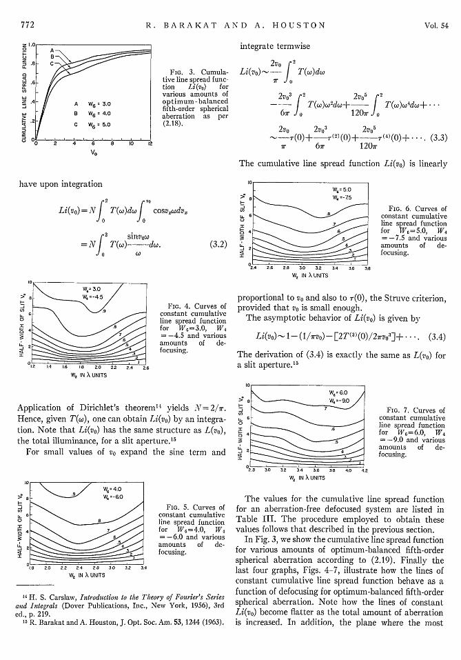
In Fig. 3, we show the cumulative line spread functionfor various amounts of optimum-balanced fifth-orderspherical aberration according to (2.19). Finally thelast four graphs, Figs. 4-7, illustrate how the lines ofconstant cumulative line spread function behave as afunction of defocusing for optimum-balanced fifth-orderspherical aberration. Note how the lines of constantLi(vo) become flatter as the total amount of aberrationis increased. In addition, the plane where the most

FIG. 3. Cumula-tive line spread func-tion Li(vo) forvarious amounts ofoptimum -balancedfifth-order sphericalaberration as per(2.18).

V0

I-

0

(3.2) U.2:

-J

*I.In0

'IFE

Vol. 54

LINE SPREAD FUNCTION

light is concentrated is not in the plane W2 determinedby (2.19), namely

W 2 = 53W6 , (3.5)

but in some other plane. For example if W6 =4.0 then,according to (3.5), the plane of best focus is W 2= 2.4.An examination of Fig. 4 indicates that the maximumconcentration of light varies according to the curveswe choose. If we choose Li(vo)=0.7, then W 2 =2.4 isthe plane of maximum energy concentration. However,

JOURNAL OF THE OPTICAL SOCIETY OF AMERICA

if we take Li(vo) = 0.9, then W2= 2.2 becomes the planeof maximum energy concentration. The situation is evenmore pronounced for W 6= 5.0, 6.0 (see Figs. 6 and 7).The same situation occurs for the total illuminancedue to a point source."

ACKNOWLEDGMENT

We wish to thank Elena Kitrosser for her help duringthe course of this investigation.

16 R. Barakat, J. Opt. Soc. Am. 51, 152 (1961).

VOLUME 54. NUMBER 6 JUNE 1964

Characteristic Functions for Special Image Formations and for a General Thick LensMAX HERZBERGER AND DONALD R. WILDER

Research Laboratories, Eastman Kodak Company, Rochester, New York 14650(Received 15 January 1964)

This paper is introductory to a study concerned with replacing the trial-and-error methods of opticaldesigning by analytical procedures. The aim is to give Hamilton's characteristic function up to any orderfor a single general lens as well as for systems that have suitable image-forming qualities. This paper laysthe groundwork for expressing various characteristic functions in terms of the optical data of the system(radii, thicknesses, indices of refraction). The theory is made practical by a technique that leads to linearequations for the system data. The characteristic functions (or, what is equivalent, their first derivatives) arederived for systems imaging one or two surfaces sharply as well as for concentric systems, to the fifth andin some cases to the seventh order. This development agrees with results previously published in closed formby Herzberger. Moreover, the characteristic function is given to the fifth order for a thick singlet withaspheric surfaces surrounded by media of arbitrary refractive index. The methods can easily be extendedto any order desired.

THE over-all objective of the work leading to thispaper has been to replace the trial-and-error

methods of lens designing by analytical procedures.Difficulties arise from the fact that the characteristicfunction of an optical system is usually not simple.Nevertheless, the basic mathematical problems arenow solved for the case of a single thick lens withaspheric surfaces immersed in media of differing re-fractive indices. The only task left is to solve certainlinear equations with algebraic coefficients, an ele-mentary, though admittedly tedious, job.

The difficulty of presenting the work lies not so muchin analyzing the problem as in reducing the formulas toa form that can be easily printed.

The method described comprises (1) finding theoptical distance between the surfaces of a thick lensand the optical distance between its vertex planes,(2) finding the optical distance between two planes foran arbitrary rotationally symmetric optical system withcertain desirable image-forming properties, and (3)equating that distance to the optical distance for thelens, for the same pair of reference planes. These opticaldistances are calculated as functions of the same vari-ables, and the coefficients of their expansions in Taylorseries are equated to each other, term by term. Thus all

possible thick lenses with the desired image-formingproperties can be obtained. The most important resultis that the problem can be reduced to a set of linearequations.

In the first section formulas are given for specialcharacteristic functions needed later in the paper, asfollows. ¶We consider the characteristic for a systemthat images one surface sharply and without distortiononto another surface and also the special case in whichtwo different surfaces are so imaged. In addition, thegeneral concentric system and the concentric systemwith special imaging qualities are discussed. ¶We makeuse of the diapoint characteristic' as a convenient tool.¶From the optical distance between two aspheric sur-faces we compute the optical distance between thevertex planes and then apply this method to the singlelens. ¶Formulas are developed for transforming thepoint characteristic into the angle characteristic, andvice versa.

Results from an earlier paper2 will simplify the de-velopment of the transformations; a still furthersimplification will be described in this paper, based on

1 M. Herzberger, Modern Geometrical Optics (Interscience Pub-lishers, Inc., New York, 1958), p. 232.

2 M. Herzberger, J. Opt. Soc. Am. 51, 135 (1961).

773June 1964