Linear Algebra Notes 1 Linear Equations 1.1 Introduction to Linear Systems Definition 1. A system of linear equations is consistent if it has at least one solution. If it has no solutions it is inconsistent. 1.2 Matrices, Vectors, and Gauss-Jordan Elimination Definition 2. Given a system of linear equations x - 3y =8 4x +9y = -2, the coefficient matrix of the system contains the coefficients of the system: 1 -3 4 9 , while the augmented matrix of the system contains the numbers to the right of the equals sign as well: 1 -3 4 9 8 -2 . Definition 3. A matrix is in reduced row-echelon form (RREF) if it satisfies all of the following conditions: a) If a row has nonzero entries, then the first nonzero entry is a 1, called a leading 1. b) If a column contains a leading 1, then all the other entries in that column are 0. c) If a row contains a leading 1, then each row above it contains a leading 1 further to the left. Definition 4. An elementary row operation (ERO) is one of the following types of operations: a) Row swap: swap two rows. b) Row division: divide a row by a (nonzero) scalar. c) Row addition: add a multiple of a row to another row. Theorem 5. For any matrix A, there is a unique matrix rref(A) in RREF which can be obtained by applying a sequence of ERO’s to A. Procedure 6. Gauss-Jordan elimination (GJE) is a procedure for putting a matrix A in RREF by applying a sequence of ERO’s. It can be applied to the augmented matrix of a system of linear equations to solve the system. Imagine a cursor moving through the entries of the augmented matrix, starting in the upper-left corner. The procedure ends when the cursor leaves the matrix. Note that steps 2, 3, and 4 consist of elementary row operations. 1
Transcript
Linear Algebra Notes
1 Linear Equations
1.1 Introduction to Linear Systems
Definition 1. A system of linear equations is consistent if it has at least one solution. If it has no solutionsit is inconsistent.
1.2 Matrices, Vectors, and Gauss-Jordan Elimination
Definition 2. Given a system of linear equations
x− 3y = 8
4x+ 9y = −2,
the coefficient matrix of the system contains the coefficients of the system:[1 −34 9
],
while the augmented matrix of the system contains the numbers to the right of the equals sign as well:[1 −34 9
∣∣∣∣ 8−2
].
Definition 3. A matrix is in reduced row-echelon form (RREF) if it satisfies all of the followingconditions:
a) If a row has nonzero entries, then the first nonzero entry is a 1, called a leading 1.
b) If a column contains a leading 1, then all the other entries in that column are 0.
c) If a row contains a leading 1, then each row above it contains a leading 1 further to the left.
Definition 4. An elementary row operation (ERO) is one of the following types of operations:
a) Row swap: swap two rows.
b) Row division: divide a row by a (nonzero) scalar.
c) Row addition: add a multiple of a row to another row.
Theorem 5. For any matrix A, there is a unique matrix rref(A) in RREF which can be obtained by applyinga sequence of ERO’s to A.
Procedure 6. Gauss-Jordan elimination (GJE) is a procedure for putting a matrix A in RREF byapplying a sequence of ERO’s. It can be applied to the augmented matrix of a system of linear equations tosolve the system.
Imagine a cursor moving through the entries of the augmented matrix, starting in the upper-left corner.The procedure ends when the cursor leaves the matrix. Note that steps 2, 3, and 4 consist of elementaryrow operations.
1
1. If the cursor column contains all 0’s, move the cursor to the right and repeat step 1.
2. If the cursor entry is 0, swap the cursor row with a lower row so that the cursor entry becomes nonzero.
3. If the cursor entry is not 1, divide the cursor row by it to make it 1.
4. If the other entries in the cursor column are nonzero, make them 0 by adding the appropriate multiplesof the cursor row to the other rows.
5. Move the cursor down and to the right and go to step 1.
1.3 On the Solutions of Linear Systems; Matrix Algebra
Definition 7. If a column of the RREF of a coefficient matrix contains a leading 1, the correspondingvariable of the linear system is called a leading variable. If a column does not contain a leading 1, thecorresponding variable is called a free variable.
Definition 8. A row of the form[0 0 · · · 0 | 1
]in the RREF of an augmented matrix is called an
inconsistent row, since it signifies the inconsistent equation 0 = 1.
Theorem 9. The number of solutions of a linear system with augmented matrix[A | b
]can be read from
rref[A | b
]:
rref[A | b
]no free variables free variable
no inconsistent rows 1 ∞inconsistent row 0 0
Definition 10 (1.3.2). The rank of a matrix A, written rank(A), is the number of leading 1’s in rref(A).
Theorem 11. For an n×m matrix A, we have rank(A) ≤ n and rank(A) ≤ m.
Proof. Each of the n rows contains at most one leading 1, as does each of the m columns.
Theorem 12 (1.3.4, uniqueness of solution with n equations and n variables). A linear system ofn equations in n variables has a unique solution if and only if the rank of its coefficient matrix A is n, inwhich case
rref(A) =
1 0 0 · · · 00 1 0 · · · 00 0 1 · · · 0...
......
. . ....
0 0 0 · · · 1
.
Proof. A system Ax = b has a unique solution if and only if it has no free variables and rref[A | b
]has
no inconsistent rows. This happens exactly when each row and each column of rref(A) contain leading 1’s,which is equivalent to rank(A) = n. The matrix above is the only n× n matrix in RREF with rank n.
Notation 13. We denote the ijth entry of a matrix A by either aij or Aij or [A]ij . (The final notation isconvenient when working with a compound matrix such as A+B.)
2
Definition 14 (1.3.5). If A and B are n×m matrices, then their sum A+B is defined entry-by-entry:
[A+B]ij = Aij +Bij .
If k is a scalar, then the scalar multiple kA of A is also defined entry-by-entry:
[kA]ij = kAij .
Definition 15 (1.3.7, Row definition of matrix-vector multiplication). The product Ax of an n×mmatrix A and a vector x ∈ Rm is given by
Ax =
− w1 −...
− wn −
x =
w1 · x...
wn · x
.
Notation 16. We denote the ith component of a vector x by either xi or [x]i. (The latter notation isconvenient when working with a compound vector such as Ax.)
Theorem 17 (1.3.8, Column definition of matrix-vector multiplication). The product Ax of an n×mmatrix A and a vector x ∈ Rm is given by
Ax =
| |v1 · · · vm| |
x1...xm
= x1v1 + · · ·+ xmvm.
Proof. According to the row definition of matrix-vector multiplication, the ith component of Ax is
[Ax]i = wi · x= ai1x1 + · · ·+ aimxm
= x1[v1]i + · · ·+ xm[vm]i
= [x1v1]i + · · ·+ [xmvm]i
= [x1v1 + · · ·+ xmvm]i.
Since Ax and x1v1 + · · ·+ xmvm have equal ith components for all i, they are equal vectors.
Definition 18 (1.3.9). A vector b ∈ Rn is called a linear combination of the vectors v1, . . . ,vm in Rn ifthere exist scalars x1, . . . , xm such that
b = x1v1 + · · ·+ xmvm.
Note that Ax is a linear combination of the columns of A. By convention, 0 is considered to be the uniquelinear combination of the empty set of vectors.
Theorem 19 (1.3.10, properties of matrix-vector multiplication). If A,B are n×m matrices, x,y ∈Rm, and k is a scalar, then
a) A(x + y) = Ax +Ay,
b) (A+B)x = Ax +Bx,
c) A(kx) = k(Ax).
3
Proof. Let wi and ui be the ith rows of A and B, respectively. We show that the ith components of eachside are equal.
[A(x + y)]i = wi · (x + y) = wi · x + wi · y = [Ax]i + [Ay]i = [Ax +Ay]i,
[(A+B)x]i = (ith row of A+B) · x = (wi + ui) · x = wi · x + ui · x = [Ax]i + [Bx]i = [Ax +Bx]i,
Definition 20 (1.3.11). A linear system with augmented matrix[A | b
]can be written in matrix form as
Ax = b.
4
2 Linear Transformations
2.1 Introduction to Linear Transformations and Their Inverses
Definition 21 (2.1.1). A function T : Rm → Rn is called a linear transformation if there exists an n×mmatrix A such that
T (x) = Ax
for all vectors x in Rm.
Note 22. If T : R2 → R2, T (x) = y =
[y1y2
], A =
[a11 a12a21 a22
], and x =
[x1x2
], then the linear transformation
above can be written as [y1y2
]=
[a11 a12a21 a22
] [x1x2
],
or y1 = a11x1 + a12x2
y2 = a21x1 + a22x2.
Definition 23. The identity matrix of size n is
In =
1 0 0 · · · 00 1 0 · · · 00 0 1 · · · 0...
......
. . ....
0 0 0 · · · 1
,
and T (x) = Inx = x is the identity transformation from Rn to Rn. If the value of n is understood,then we often write just I for In.
Definition 24. The standard (basis) vectors e1, e2, . . . , em in Rm are the vectors ei =
00...1...0
, with a 1 in
the ith place and 0’s elsewhere. Note that for a matrix A with m columns, Aei is the ith column of A.
Theorem 25 (2.1.2, matrix of a linear transformation). For a linear transformation T : Rm → Rn,there is a unique matrix A such that T (x) = Ax, obtained by applying T to the standard basis vectors:
A =
| | |T (e1) T (e2) · · · T (em)| | |
.It follows that if two n×m matrices A and B satisfy Ax = Bx for all x ∈ Rm, then A = B.
Proof. By the definition of matrix-vector multiplication, the ith column of A is Aei = T (ei). For the secondstatement, note that if Ax = Bx for all x ∈ Rm, then A and B define the same linear transformation T , sothey must be the same matrix by the first part of the theorem.
5
Theorem 26 (2.1.3, linearity criterion). A function T : Rm → Rn is a linear transformation if andonly if
a) T (v + w) = T (v) + T (w), for all vectors v and w in Rm, and
b) T (kv) = kT (v), for all vectors v in Rm and all scalars k.
Proof. Suppose T is a linear transformation, and let A be a matrix such that T (x) = Ax for all x ∈ Rm.Then
T (v + w) = A(v + w) = Av +Aw = T (v) + T (w),
T (kv) = A(kv) = k(Av) = kT (v).
To prove the converse, suppose that a function T : Rm → Rn satisfies (a) and (b). Then for all x ∈ Rm,
T (x) = T
x1x2...xm
= T (x1e1 + x2e2 + · · ·+ xmem)
= T (x1e1) + T (x2e2) + · · ·+ T (xmem)
= x1T (e1) + x2T (e2) + · · ·+ xmT (em)
=
| | |T (e1) T (e2) · · · T (em)| | |
x1x2...xm
,so T is a linear transformation.
2.2 Linear Transformations in Geometry
Definition 27. The linear transformation from R2 to R2 represented by a matrix of the form A =
[k 00 k
]is called scaling by (a factor of) k.
Definition 28 (2.2.1). Given a line L through the origin in R2 parallel to the vector w, the orthogonalprojection onto L is the linear transformation
projL(x) =( x ·w
w ·w
)w,
with matrix1
w21 + w2
2
[w2
1 w1w2
w1w2 w22
].
The projections onto the x- and y-axes are represented by the matrices
[1 00 0
]and
[0 00 1
], respectively.
Definition 29 (2.2.2). Given a line L through the origin in R2 parallel to the vector w, the reflectionabout L is the linear transformation
refL(x) = 2 projL(x)− x = 2( x ·w
w ·w
)w − x,
6
with matrix1
w21 + w2
2
[2w2
1 − 1 2w1w2
2w1w2 2w22 − 1
].
The reflections about the x- and y-axes are represented by the matrices
[1 00 −1
]and
[−1 00 1
], respectively.
Definition 30 (2.2.3). The linear transformation from R2 to R2 represented by a matrix of the form
A =
[cos θ − sin θsin θ cos θ
]is called counterclockwise rotation through an angle θ (about the origin).
Definition 31 (2.2.5). The linear transformation from R2 to R2 represented by a matrix of the form
A =
[1 k0 1
]or A =
[1 0k 1
]is called a horizontal shear or a vertical shear, respectively.
2.3 Matrix Products
Theorem 32. If T : Rm → Rp and S : Rp → Rn are linear transformations, then their compositionS T : Rm → Rn given by
(S T )(x) = S(T (x))
is also a linear transformation.
Proof. We show that if T and S satisfy the linearity criteria, then so does S T . Let v, w ∈ Rm and k ∈ R.Then
(S T )(v + w) = S(T (v + w)) = S(T (v) + T (w)) = S(T (v)) + S(T (w)) = (S T )(v) + (S T )(w),
(S T )(kv) = S(T (kv)) = S(kT (v)) = k(S(T (v)) = k(S T )(v).
Definition 33 (2.3.1, matrix multiplication from composition of linear transformations). If B isan n× p matrix and A is a q ×m matrix, then the product matrix BA is defined if and only if p = q, inwhich case it is the matrix of the linear transformation T (x) = B(A(x)). As a result, (BA)x = B(A(x)).
Theorem 34 (2.3.2, matrix multiplication using columns of matrix on the right). If B is an n× pmatrix and A is a p×m matrix with columns v1, . . . ,vm, then
BA = B
| | |v1 v2 · · · vm| | |
=
| | |Bv1 Bv2 · · · Bvm| | |
.Proof. The ith column of BA is (BA)ei = B(Aei) = Bvi.
7
Theorem 35 (2.3.4, matrix multiplication entry-by-entry). If B is an n× p matrix and A is a p×mmatrix with columns v1, . . . ,vm, then the ijth entry of
BA =
− w1 −...
− wi −...
− wn −
| | |
v1 · · · vj · · · vm| | |
is the dot product of the ith row of B with the jth column of A:
Proof. The ijth entry of BA is the ith component of Bvj , by Theorem 34, which equals wi ·vj , by Definition15.
Theorem 36 (2.3.5, identity matrix). For any n×m matrix A,
AIm = A and InA = A.
Proof. Since (AIm)x = A(Imx) = Ax for all x ∈ Rm, we have AIm = A. The proof for InA = A isanalogous.
Theorem 37 (2.3.6, multiplication is associative). If AB and BC are defined, then (AB)C = A(BC).We can simply write ABC to indicate this single matrix.
for any x of appropriate dimension, so (AB)C = A(BC).
Theorem 38 (2.3.7, multiplication distributes over addition). If A and B are n× p matrices and Cand D are p×m matrices, then
A(C +D) = AC +AD,
(A+B)C = AC +BC.
Proof. We show that the two sides of the first equation give the same linear transformation, using parts aand b of Theorem 19. Because of Theorem 37, we can suppress some parentheses:
A(C +D)x = A(Cx +Dx) = ACx +ADx = (AC +AD)x.
Similarly,(A+B)Cx = ACx +BCx = (AC +BC)x.
Theorem 39 (2.3.8, scalar multiplication). If A is an n × p matrix, B is a p ×m matrix, and k is ascalar, then
k(AB) = (kA)B and k(AB) = A(kB).
Note 40 (2.3.3, multiplication is not commutative). When A and B are both n×m matrices, AB andBA are both defined, but they are usually not equal. In fact, they do not even have the same dimensionsunless n = m.
8
2.4 The Inverse of a Linear Transformation
Definition 41. For a function T : X → Y , X is called the domain and Y is called the target.
• A function T : X → Y is called one-to-one if for any y ∈ Y there is at most one input x ∈ X suchthat T (x) = y (different inputs give different outputs).
• A function T : X → Y is called onto if for any y ∈ Y there is at least one input x ∈ X such thatT (x) = y (every target element is an output).
• A function T : X → Y is called invertible if for any y ∈ Y there is exactly one x ∈ X such thatT (x) = y. Note that a function is invertible if and only if it is both one-to-one and onto.
Definition 42 (2.4.1). If T : X → Y is invertible, we can define a unique inverse function T−1 : Y → Xby setting T−1(y) to be the unique x ∈ X such that T (x) = y. It follows that
T−1(T (x)) = x and T (T−1(y)) = y,
so T−1 T and T T−1 are identity functions. For any invertible function T , (T−1)−1 = T , so T−1 is alsoinvertible, with inverse function T .
Note 43. A linear transformation T : Rm → Rn given by T (x) = Ax is invertible if for any y ∈ Rn, thereis a unique x ∈ Rm such that Ax = y.
Theorem 44 (2.4.2, linearity of the inverse). If a linear transformation T : Rm → Rn is invertible, thenits inverse T−1 is also a linear transformation.
Proof. We show that if T satisfies the linearity criteria (Theorem 26), then T−1 : Rn → Rm does also. Letv,w ∈ Rn and k ∈ R. Then
v + w = T (T−1(v)) + T (T−1(w)) = T (T−1(v) + T−1(w)),
and applying T−1 to each side gives
T−1(v + w) = T−1(v) + T−1(w).
Similarly,kv = kT (T−1(v)) = T (kT−1(v)),
and soT−1(kv) = kT−1(v).
Definition 45 (2.4.2). If T (x) = Ax is invertible, then A is said to be an invertible matrix, and thematrix of T−1 is called the inverse matrix of A, written A−1.
Theorem 46 (2.4.8, the inverse matrix as multiplicative inverse). A is invertible if and only if thereexists a matrix B such that BA = I and AB = I. In this case, B = A−1.
9
Proof. If A is invertible, then, taking B to be A−1,
(BA)x = (A−1A)x = A−1(Ax) = T−1(T (x)) = x = Ix
(AB)y = (AA−1)y = A(A−1y) = T (T−1(y)) = y = Iy
for all x,y of correct dimension, so BA = I and AB = I.Conversely, if we have a matrix B such that BA = I and AB = I, then T (x) = Ax and S(y) = By
satisfy
S(T (x)) = B(Ax) = (BA)x = Ix = x,
T (S(y)) = A(By) = (AB)y = Iy = y,
for any x,y of correct dimension, so S T and T S are identity transformations. Thus S is the inversetransformation of T , A is invertible, and B = A−1.
Theorem 47 (2.4.3, invertibility criteria). If a matrix is not square, then it is not invertible. For ann× n matrix A, the following are equivalent:
1. A is invertible,
2. Ax = b has a unique solution x for any b,
3. rref(A) = In,
4. rank(A) = n.
Proof. Let A be an n × m matrix with inverse A−1. Since T (x) = Ax maps Rm → Rn, the inversetransformation T−1 maps Rn → Rm, so A−1 is an m× n matrix. If m > n, then the linear system Ax = 0has at least one free variable, so it cannot have a unique solution, contradicting the invertibility of A. Ifn > m, then A−1y = 0 has at least one free variable, so it cannot have a unique solution, contradicting theinvertibility of A−1. It follows that n = m.
The equivalence of the first two statements is a restatement of Note 43. Statements 3 and 4 are equivalentto the second one by Theorem 12.
Procedure 48 (2.4.5, computing the inverse of a matrix). To find the inverse of a matrix A (if itexists), compute rref
[A | In
], which is equal to
[rref(A) | B
]for some B.
• If rref(A) 6= In, then A is not invertible.
• If rref(A) = In, then A is invertible and A−1 = B.
Theorem 49 (2.4.9, inverse of a 2 × 2 matrix). A 2 × 2 matrix A =
[a bc d
]is invertible if and only if
ad− bc 6= 0. The scalar ad− bc is called the determinant of A, written det(A). If A =
[a bc d
]is invertible,
then
A−1 =1
det(A)
[d −b−c a
].
Theorem 50 (2.4.7, inverse of a product of matrices). If A and B are invertible n × n matrices,then AB is invertible as well, and
(AB)−1 = B−1A−1.
10
Proof. To show that B−1A−1 is the inverse of AB, we check that their product in either order is the identitymatrix:
(AB)(B−1A−1) = A(BB−1)A−1 = AInA−1 = AA−1 = In,
(B−1A−1)(AB) = B−1(A−1A)B = B−1InB = B−1B = In.
11
3 Subspaces of Rn and Their Dimensions
3.1 Image and Kernel of a Linear Transformation
Definition 51 (3.1.1). The image of a function T : X → Y is its set of outputs:
im(T ) = T (x) : x ∈ X,
a subset of the target Y . Note that T is onto if and only if im(T ) = Y .For a linear transformation T : Rm → Rn, the image is
im(T ) = T (x) : x ∈ Rm,
a subset of the target Rn.
Definition 52 (3.1.2). The set of all linear combinations of the vectors v1, . . . ,vm in Rn is called theirspan:
If span(v1,v2, . . . ,vm) = W for some subset W of Rn, we say that the vectors v1, . . . ,vm span W . Thusspan can be used as a noun or as a verb.
Theorem 53 (3.1.3). The image of a linear transformation T (x) = Ax is the span of the column vectors ofA. We denote the image of T by im(T ) or im(A).
Proof. By the column definition of matrix multiplication,
T (x) = Ax =
| |v1 · · · vm| |
x1...xm
= x1v1 + · · ·+ xmvm.
Thus the image of T consists of all linear combinations of the column vectors v1, . . . ,vm of A.
Note 54. By the preceding theorem, the column vectors v1, . . . ,vm ∈ Rn of an n×m matrix A span Rn ifand only if im(A) = Rn, which is equivalent to T (x) = Ax being onto.
Theorem 55 (3.1.4, the image is a subspace). The image of a linear transformation T : Rm → Rnhas the following properties:
a) contains zero vector: 0 ∈ im(T ).
b) closed under addition: If y1,y2 ∈ im(T ), then y1 + y2 ∈ im(T ).
c) closed under scalar multiplication: If y ∈ im(T ) and k ∈ R, then ky ∈ im(T ).
As we will see in the next section, these three properties mean that im(T ) is a subspace.
Proof.
a) 0 = A0 = T (0) ∈ im(T ).
b) There exist vectors x1,x2 ∈ Rm such that T (x1) = y1, T (x2) = y2. Since T is linear, y1 + y2 =T (x1) + T (x2) = T (x1 + x2) ∈ im(T ).
c) There exists a vector x ∈ Rm such that T (x) = y. Since T is linear, ky = kT (x) = T (kx) ∈ im(T ).
12
Definition 56 (3.1.1). The kernel of a linear transformation T : Rm → Rn is its set of zeros:
ker(T ) = x ∈ Rm : T (x) = 0,
a subset of the domain Rm.
Theorem 57 (kernel criterion for one-to-one). A linear transformation T : Rm → Rn is one-to-one ifand only if ker(T ) = 0.
Proof. Since T (x) = Ax for some A, we have T (0) = A0 = 0. If T is one-to-one, it follows immediately that0 is the only solution of T (x) = 0, so ker(T ) = 0.
Conversely, suppose ker(T ) = 0, and let x1,x2 ∈ Rm satisfy T (x1) = y and T (x2) = y. By thelinearity of T ,
T (x1 − x2) = T (x1)− T (x2) = y − y = 0,
so x1 − x2 = 0 and x1 = x2, proving that T is one-to-one.
Definition 58 (3.2.6). A linear relation among the vectors v1, . . . ,vm ∈ Rn is an equation of the form
c1v1 + · · ·+ cmvm = 0
for scalars c1, . . . , cm ∈ R. If c1 = · · · = cm = 0, the relation is called trivial, while if at least one of the ciin nonzero, the relation is nontrivial.
Theorem 59. The kernel of a linear transformation T (x) = Ax is the set of solutions x of the equationAx = 0, i.e. | |
v1 · · · vm| |
x1...xm
= 0,
which corresponds to the set of linear relations x1v1 + · · ·+ xmvm among the column vectors v1, . . . ,vm ofA. We denote the kernel of T by ker(T ) or ker(A).
Proof. The first statement is immediate from the definition of kernel, while the correspondence with linearrelations follows from the column definition of the product Ax.
Theorem 60 (3.1.4, the kernel is a subspace). The kernel of a linear transformation T : Rm → Rnhas the following properties:
a) contains zero vector: 0 ∈ ker(T ).
b) closed under addition: If x1,x2 ∈ ker(T ), then x1 + x2 ∈ ker(T ).
c) closed under scalar multiplication: If x ∈ ker(T ) and k ∈ R, then kx ∈ ker(T ).
As we will see in the next section, these three properties mean that ker(T ) is a subspace.
Proof.
a) T (0) = A0 = 0.
b) Since T is linear, T (x1 + x2) = T (x1) + T (x2) = 0 + 0 = 0.
c) Since T is linear, T (kx) = kT (x) = k0 = 0.
13
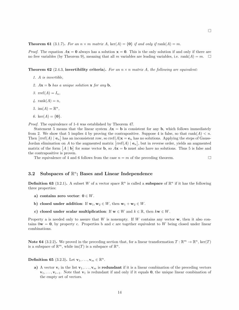
Theorem 61 (3.1.7). For an n×m matrix A, ker(A) = 0 if and only if rank(A) = m.
Proof. The equation Ax = 0 always has a solution x = 0. This is the only solution if and only if there areno free variables (by Theorem 9), meaning that all m variables are leading variables, i.e. rank(A) = m.
Theorem 62 (2.4.3, invertibility criteria). For an n× n matrix A, the following are equivalent:
1. A is invertible,
2. Ax = b has a unique solution x for any b,
3. rref(A) = In,
4. rank(A) = n,
5. im(A) = Rn,
6. ker(A) = 0.
Proof. The equivalence of 1-4 was established by Theorem 47.Statement 5 means that the linear system Ax = b is consistent for any b, which follows immediately
from 2. We show that 5 implies 4 by proving the contrapositive. Suppose 4 is false, so that rank(A) < n.Then
[rref(A) | en
]has an inconsistent row, so rref(A)x = en has no solutions. Applying the steps of Gauss-
Jordan elimination on A to the augmented matrix[rref(A) | en
], but in reverse order, yields an augmented
matrix of the form[A | b
]for some vector b, so Ax = b must also have no solutions. Thus 5 is false and
the contrapositive is proven.The equivalence of 4 and 6 follows from the case n = m of the preceding theorem.
3.2 Subspaces of Rn; Bases and Linear Independence
Definition 63 (3.2.1). A subset W of a vector space Rn is called a subspace of Rn if it has the followingthree properties:
a) contains zero vector: 0 ∈W .
b) closed under addition: If w1,w2 ∈W , then w1 + w2 ∈W .
c) closed under scalar multiplication: If w ∈W and k ∈ R, then kw ∈W .
Property a is needed only to assure that W is nonempty. If W contains any vector w, then it also con-tains 0w = 0, by property c. Properties b and c are together equivalent to W being closed under linearcombinations.
Note 64 (3.2.2). We proved in the preceding section that, for a linear transformation T : Rm → Rn, ker(T )is a subspace of Rm, while im(T ) is a subspace of Rn.
Definition 65 (3.2.3). Let v1, . . . ,vm ∈ Rn.
a) A vector vi in the list v1, . . . ,vm is redundant if it is a linear combination of the preceding vectorsv1, . . . ,vi−1. Note that v1 is redundant if and only if it equals 0, the unique linear combination ofthe empty set of vectors.
14
b) The vectors v1, . . . ,vm are called linearly independent (LI) if none of them are redundant. Oth-erwise, they are linearly dependent (LD).
c) The vectors v1, . . . ,vm form a basis of a subspace V of Rn if they span V and are linearly independent.
Theorem 66 (3.2.7, linear dependence criterion). The vectors v1, . . . ,vm ∈ Rn are linearly dependentif and only if there exists an nontrivial (linear) relation among them.
Proof. Suppose v1, . . . ,vm are linearly dependent and let vi = c1v1 + · · ·+ ci−1vi−1 be a redundant vectorin this list. Then we obtain a nontrivial relation by subtracting vi from both sides:
c1v1 + · · ·+ ci−1vi−1 + (−1)vi = 0.
Conversely, if there is a nontrivial relation c1v1 + · · · + civi + · · · + cmvm = 0, where i is the highestindex such that ci 6= 0, then we can solve for vi to show that vi is redundant:
vi = −c1ci
v1 − · · · −ci−1ci
vi−1.
Thus the vectors v1, . . . ,vm are linearly dependent.
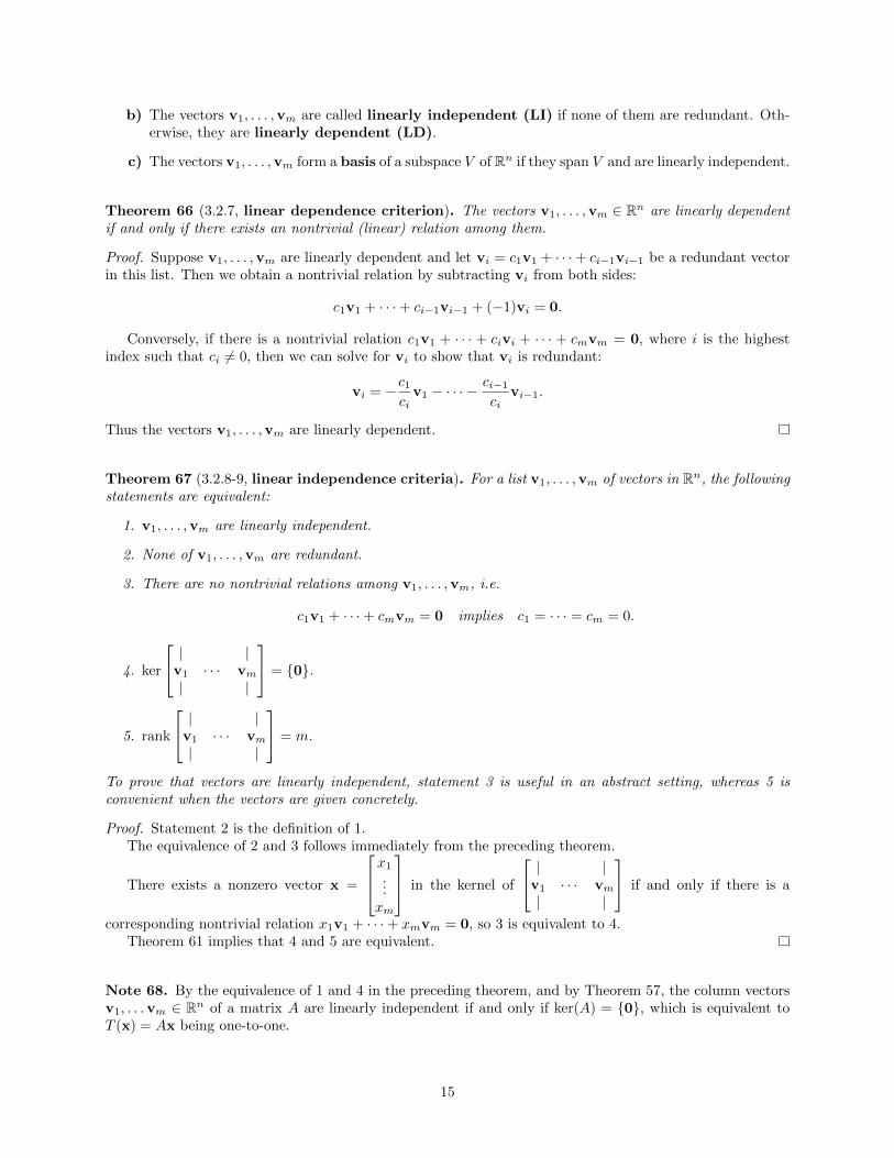
Theorem 67 (3.2.8-9, linear independence criteria). For a list v1, . . . ,vm of vectors in Rn, the followingstatements are equivalent:
1. v1, . . . ,vm are linearly independent.
2. None of v1, . . . ,vm are redundant.
3. There are no nontrivial relations among v1, . . . ,vm, i.e.
To prove that vectors are linearly independent, statement 3 is useful in an abstract setting, whereas 5 isconvenient when the vectors are given concretely.
Proof. Statement 2 is the definition of 1.The equivalence of 2 and 3 follows immediately from the preceding theorem.
There exists a nonzero vector x =
x1...xm
in the kernel of
| |v1 · · · vm| |
if and only if there is a
corresponding nontrivial relation x1v1 + · · ·+ xmvm = 0, so 3 is equivalent to 4.Theorem 61 implies that 4 and 5 are equivalent.
Note 68. By the equivalence of 1 and 4 in the preceding theorem, and by Theorem 57, the column vectorsv1, . . .vm ∈ Rn of a matrix A are linearly independent if and only if ker(A) = 0, which is equivalent toT (x) = Ax being one-to-one.
15
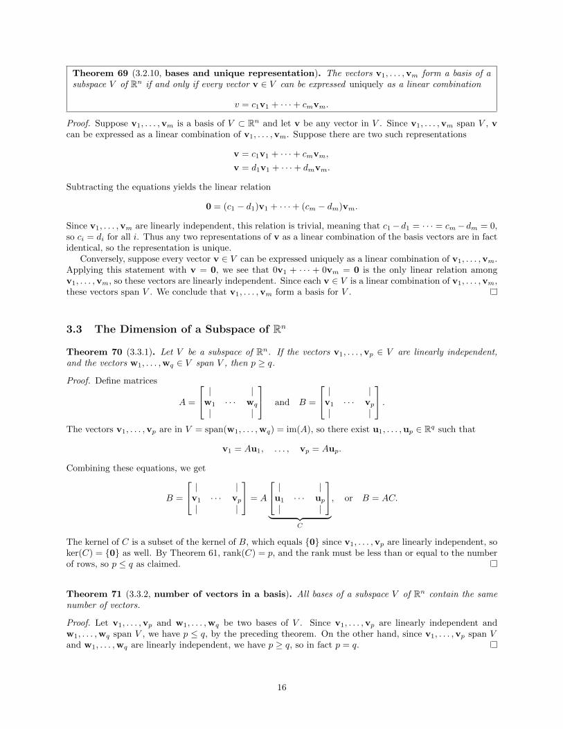
Theorem 69 (3.2.10, bases and unique representation). The vectors v1, . . . ,vm form a basis of asubspace V of Rn if and only if every vector v ∈ V can be expressed uniquely as a linear combination
v = c1v1 + · · ·+ cmvm.
Proof. Suppose v1, . . . ,vm is a basis of V ⊂ Rn and let v be any vector in V . Since v1, . . . ,vm span V , vcan be expressed as a linear combination of v1, . . . ,vm. Suppose there are two such representations
v = c1v1 + · · ·+ cmvm,
v = d1v1 + · · ·+ dmvm.
Subtracting the equations yields the linear relation
0 = (c1 − d1)v1 + · · ·+ (cm − dm)vm.
Since v1, . . . ,vm are linearly independent, this relation is trivial, meaning that c1− d1 = · · · = cm− dm = 0,so ci = di for all i. Thus any two representations of v as a linear combination of the basis vectors are in factidentical, so the representation is unique.
Conversely, suppose every vector v ∈ V can be expressed uniquely as a linear combination of v1, . . . ,vm.Applying this statement with v = 0, we see that 0v1 + · · · + 0vm = 0 is the only linear relation amongv1, . . . ,vm, so these vectors are linearly independent. Since each v ∈ V is a linear combination of v1, . . . ,vm,these vectors span V . We conclude that v1, . . . ,vm form a basis for V .
3.3 The Dimension of a Subspace of Rn
Theorem 70 (3.3.1). Let V be a subspace of Rn. If the vectors v1, . . . ,vp ∈ V are linearly independent,and the vectors w1, . . . ,wq ∈ V span V , then p ≥ q.
Proof. Define matrices
A =
| |w1 · · · wq
| |
and B =
| |v1 · · · vp| |
.The vectors v1, . . . ,vp are in V = span(w1, . . . ,wq) = im(A), so there exist u1, . . . ,up ∈ Rq such that
v1 = Au1, . . . , vp = Aup.
Combining these equations, we get
B =
| |v1 · · · vp| |
= A
| |u1 · · · up| |
︸ ︷︷ ︸
C
, or B = AC.
The kernel of C is a subset of the kernel of B, which equals 0 since v1, . . . ,vp are linearly independent, soker(C) = 0 as well. By Theorem 61, rank(C) = p, and the rank must be less than or equal to the numberof rows, so p ≤ q as claimed.
Theorem 71 (3.3.2, number of vectors in a basis). All bases of a subspace V of Rn contain the samenumber of vectors.
Proof. Let v1, . . . ,vp and w1, . . . ,wq be two bases of V . Since v1, . . . ,vp are linearly independent andw1, . . . ,wq span V , we have p ≤ q, by the preceding theorem. On the other hand, since v1, . . . ,vp span Vand w1, . . . ,wq are linearly independent, we have p ≥ q, so in fact p = q.
16
Definition 72 (3.3.3). The number of vectors in a basis of a subspace V of Rn is called the dimension ofV , denoted dim(V ).
Note 73. It can easily be shown that the standard basis vectors e1, . . . , en of Rn do in fact form a basis ofRn, so that, as would be expected, dim(Rn) = n.
Theorem 74 (3.3.4, size of linearly independent and spanning sets). Let V be a subspace of Rn withdim(V ) = m.
a) Any linearly independent set of vectors in V contains at most m vectors. If it contains exactly mvectors, then it forms a basis of V .
b) Any spanning set of vectors in V contains at least m vectors. If it contains exactly m vectors, then itforms a basis of V .
Proof.
a) Suppose v1, . . . ,vp are linearly independent vectors in V and w1, . . . ,wm form a basis of V . Thenw1, . . . ,wm span V , so p ≤ m by Theorem 70.
Now let v1, . . . ,vm be linearly independent vectors in V . To prove that v1, . . . ,vm form a basis of V ,we must show that any vector v ∈ V is contained the span of v1, . . . ,vm. By what we have alreadyshown, the m+ 1 vectors v1, . . . ,vm,v must be linearly dependent. Since no vi is redundant in thislist, v must be redundant, meaning that v is a linear combination of v1, . . . ,vm, as needed.
b) Suppose v1, . . . ,vq span V and w1, . . . ,wm form a basis of V . Then w1, . . . ,wm are linearly inde-pendent, so q ≥ m by Theorem 70.
Now let v1, . . . ,vm be vectors which span V . To prove that v1, . . . ,vm form a basis of V , we mustshow that they are linearly independent. We use proof by contradiction. Suppose that v1, . . . ,vmare linearly dependent, with some redundant vi, so that vi = c1v1 + · · ·+ ci−1vi−1 for some scalarsc1, . . . , ci−1. In any linear combination v = d1v1 + · · ·+ dmvm, we can substitute for vi to rewrite vas a linear combination of the other vectors:
We conclude that the subspace V = span(v1, . . . ,vm) of dimension m is in fact spanned by just m−1vectors, a contradiction.
Procedure 75 (finding a basis of the kernel). The kernel of a matrix A consists of all solutions x tothe equation Ax = 0. To find a basis of the kernel of A, solve Ax = 0, using Gauss-Jordan eliminationto compute rref
[A | 0
]=[rref(A) | 0
], solving the resulting system of linear equations for the leading
variables, and substituting parameters r, s, t, etc. for the free variables. Then write the general solution asa linear combination of constant vectors with the parameters as coefficients. These constant vectors form abasis for ker(A).
Procedure 76 (3.3.5, finding a basis of the image). To obtain a basis of the image of A, take thecolumns of A corresponding to the columns of rref(A) containing leading 1’s.
Definition 77. The nullity of a matrix A, written nullity(A), is the dimension of the kernel of A.
17
Theorem 78. For any matrix A, rank(A) = dim(imA).
Proof. By Procedure 76, a basis of im(A) contains as many vectors as the number of leading 1’s in rref(A),which is the definition of rank(A).
Theorem 79 (3.3.7, Rank-Nullity Theorem). For any n×m matrix A,
dim(kerA) + dim(imA) = m.
In terms of the linear transformation T : Rm → Rn given by T (x) = Ax, this can be written as
dim(kerT ) + dim(imT ) = dim(Rm).
In terms of nullity and rank, we have
nullity(A) + rank(A) = m.
Proof. From Procedure 75, we know that a basis of ker(A) contains a vector for each free variable of A.From Procedure 76, we know that a basis of im(A) contains a vector for each leading variable of A. Sincethe number of free variables plus the number of leading variables equals the total number of variables m, thefirst equation holds. The final two equations then follow from the definitions and the preceding theorem.
Theorem 80 (3.3.10, invertibility criteria). For an n× n matrix A =
| |v1 · · · vn| |
, the following are
equivalent:
1. A is invertible,
2. Ax = b has a unique solution x for any b,
3. rref(A) = In,
4. rank(A) = n,
5. im(A) = Rn,
6. ker(A) = 0,
7. v1, . . . ,vn span Rn,
8. v1, . . . ,vn are linearly independent,
9. v1, . . . ,vn form a basis of Rn.
Proof. Statements 1-6 are equivalent by Theorem 62. Statements 5 and 7 are equivalent by Note 54. State-ments 6 and 8 are equivalent by Note 68. Statements 7, 8, and 9 are equivalent by Theorem 74.
18
3.4 Coordinates
Definition 81 (3.4.1). Consider a basis B = (v1,v2, . . . ,vm) of a subspace V of Rn. By Theorem 69, anyvector x ∈ V can be written uniquely as
x = c1v1 + c2v2 + · · ·+ cmvm.
The scalars c1, c2, . . . , cm are called the B-coordinates of x, and
[x]B =
c1c2...cm
is the B-coordinate vector of x.
Note 82. If we let S = SB =
| |v1 · · · vm| |
, then the relationship between x and [x]B is given by
x = c1v1 + · · ·+ cmvm =
| |v1 · · · vm| |
c1...cm
= S[x]B.
Note 83. For the standard basis E = (e1, . . . , en) of Rn, the E-coordinate vector of a vector x ∈ Rn is justx itself, since
x =
x1...xn
= x1e1 + · · ·+ xnen.
In terms of the preceding note, SE =
| |e1 · · · en| |
= I, so that x = I[x]E = [x]E .
Theorem 84 (3.4.2, linearity of coordinates). If B is a basis of a subspace V of Rn, then for all x,y ∈ Vand k ∈ R:
a) [x + y]B = [x]B + [y]B,
b) [kx]B = k[x]B.
Proof. Let B = (v1, . . . ,vm).
a) If x = c1v1 + · · ·+ cmvm and y = d1v1 + · · ·+ dmvm, then x + y = (c1 + d1)v1 + · · ·+ (cm + dm)vm,so that
[x + y]B =
c1 + d1...
cm + dm
=
c1...cm
+
d1...dm
= [x]B + [y]B.
b) If x = c1v1 + · · ·+ cmvm, then kx = kc1v1 + · · ·+ kcmvm, so that
[kx]B =
kc1...kcm
= k
c1...cm
= k[x]B.
19
Theorem 85 (3.4.3, B-matrix of a linear transformation). Consider a linear transformation T : Rn →Rn and a basis B = (v1, . . . ,vn) of Rn. Then for any x ∈ Rn, the B-coordinate vectors of x and of T (x) arerelated by the equation
[T (x)]B = B[x]B,
where
B =
| |[T (v1)]B · · · [T (vn)]B| |
,the B-matrix of T . In other words, taking either path in the following diagram yields the same result (wesay that the diagram commutes):
x = c1v1 + · · ·+ cnvnT−−−−−−−−−→ T (x)y y
[x]B =
c1...cm
B−−−−−−−−−→ [T (x)]B
Proof. Write x as a linear combination x = c1v1 + · · · + cnvn of the vectors in the basis B. We use thelinearity of T to compute
T (x) = T (c1v1 + · · ·+ cnvn) = c1T (v1) + · · ·+ cnT (vn).
Taking the B-coordinate vector of each side and using the linearity of coordinates, we get
[T (x)]B = [c1T (v1) + · · ·+ cnT (vn)]B
= c1[T (v1)]B + · · ·+ cn[T (vn)]B
=
| |[T (v1)]B · · · [T (vn)]B| |
c1...cn
= B[x]B.
Note 86. For the standard basis E = (e1, . . . , en) of Rn, the E-matrix of a linear transformation T : Rn → Rngiven by T (x) = Ax is just A, the standard matrix of T . In terms of the preceding theorem, | |
[T (v1)]E · · · [T (vn)]E| |
=
| |T (v1) · · · T (vn)| |
= A.
In this case, the diagram above becomes:
x = x1e1 + · · ·+ xnenT−−−−−−−−−→ T (x)∥∥∥ ∥∥∥
[x]E =
x1...xm
A−−−−−−−−−→ [T (x)]E
20
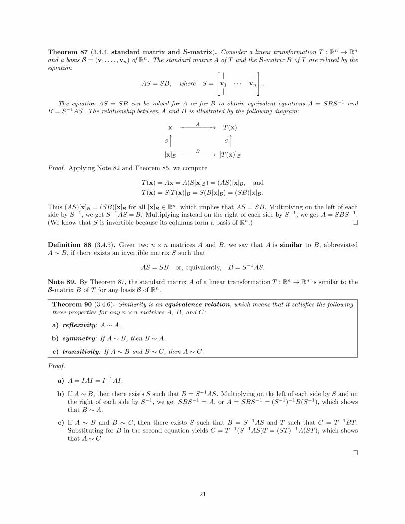
Theorem 87 (3.4.4, standard matrix and B-matrix). Consider a linear transformation T : Rn → Rnand a basis B = (v1, . . . ,vn) of Rn. The standard matrix A of T and the B-matrix B of T are related by theequation
AS = SB, where S =
| |v1 · · · vn| |
.The equation AS = SB can be solved for A or for B to obtain equivalent equations A = SBS−1 and
B = S−1AS. The relationship between A and B is illustrated by the following diagram:
xA−−−−−−−−−→ T (x)
S
x S
x[x]B
B−−−−−−−−−→ [T (x)]B
Proof. Applying Note 82 and Theorem 85, we compute
T (x) = Ax = A(S[x]B) = (AS)[x]B, and
T (x) = S[T (x)]B = S(B[x]B) = (SB)[x]B.
Thus (AS)[x]B = (SB)[x]B for all [x]B ∈ Rn, which implies that AS = SB. Multiplying on the left of eachside by S−1, we get S−1AS = B. Multiplying instead on the right of each side by S−1, we get A = SBS−1.(We know that S is invertible because its columns form a basis of Rn.)
Definition 88 (3.4.5). Given two n × n matrices A and B, we say that A is similar to B, abbreviatedA ∼ B, if there exists an invertible matrix S such that
AS = SB or, equivalently, B = S−1AS.
Note 89. By Theorem 87, the standard matrix A of a linear transformation T : Rn → Rn is similar to theB-matrix B of T for any basis B of Rn.
Theorem 90 (3.4.6). Similarity is an equivalence relation, which means that it satisfies the followingthree properties for any n× n matrices A, B, and C:
a) reflexivity: A ∼ A.
b) symmetry: If A ∼ B, then B ∼ A.
c) transitivity: If A ∼ B and B ∼ C, then A ∼ C.
Proof.
a) A = IAI = I−1AI.
b) If A ∼ B, then there exists S such that B = S−1AS. Multiplying on the left of each side by S and onthe right of each side by S−1, we get SBS−1 = A, or A = SBS−1 = (S−1)−1B(S−1), which showsthat B ∼ A.
c) If A ∼ B and B ∼ C, then there exists S such that B = S−1AS and T such that C = T−1BT .Substituting for B in the second equation yields C = T−1(S−1AS)T = (ST )−1A(ST ), which showsthat A ∼ C.
21
4 Linear Spaces
4.1 Introduction to Linear Spaces
Definition 91 (4.1.1). A linear space V (more commonly known as a vector space) is a set V togetherwith an addition rule and a scalar multiplication rule:
• For f, g ∈ V , there is an element f + g ∈ V .
• For f ∈ V and k ∈ R, there is an element kf ∈ V .
which satisfy the following eight properties (for all f, g, h ∈ V and c, k ∈ R):
1. addition is associative: (f + g) + h = f + (g + h).
2. addition is commutative: f + g = g + f .
3. an additive identity exists (a neutral element): There is an element n ∈ V such that f + n = ffor all f ∈ V . This n is unique and is denoted by 0.
4. additive inverses exist: For each f ∈ V , there exists a g ∈ V such that f + g = 0. This g is uniqueand is denoted by (−f).
5. s.m. distributes over addition in V : k(f + g) = kf + kg.
6. s.m. distributes over addition in R: (c+ k)f = cf + kf .
7. s.m. is “associative”: c(kf) = (ck)f .
8. an “identity” exists for s.m.: 1f = f .
Note 92. Vector spaces Rn and their subspaces W ⊂ Rn are examples of linear spaces. Linear spacesare generalizations of Rn. Using the addition and scalar multiplication operations, we can construct linearcombinations, which then enable us to define the basic notions of linear algebra (which we have alreadydefined for Rn): subspace, span, linear independence, basis, dimension, coordinates, linear transformation,image, kernel, matrix of a transformation, etc.
Note 93. Typically, both Rn and the linear spaces defined above are referred to as vector spaces. If it isnecessary to draw a distinction, then the latter are called abstract vector spaces. When one is first learninglinear algebra, this terminology is potentially confusing because the elements of most “abstract vector spaces”are not vectors in the traditional sense, but functions, or polynomials, or sequences, etc. Thus we will followthe text in speaking of vector spaces Rn and linear spaces V .
Definition 94.
• The set F (R,R) of all functions f : R→ R (real-valued functions of the real numbers) is a linear space.
• The set C∞ of all functions f : R → R which can be differentiated any number of times (smoothfunctions) is a linear space. It includes all polynomials, exponential functions, sin(x), cos(x), etc.
• The set P of all polynomials (with real coefficients) is a linear space.
• The set Pn of all polynomials of degree ≤ n is a linear space.
• The set Rn×m of n×m matrices with real coefficients is a linear space.
Definition 95 (4.1.2). A subset W of a linear space V is called a subspace of V if it satisfies the followingthree properties:
22
a) contains neutral element: 0 ∈W .
b) closed under addition: If f, g ∈W , then f + g ∈W .
c) closed under scalar multiplication: If f ∈W and k ∈ R, then kf ∈W .
Theorem 96. A subspace W of a linear space V is itself a linear space.
Proof. Property a guarantees that W contains the neutral element from V , which is property 3 of a linearspace.
For property 4 of a linear space, first note that for any f ∈ V , 0f = (0+0)f = 0f +0f , and so 0 = 0f . Itfollows that we can write the additive inverse as −f = (−1)f , since f+(−1)f = 1f+(−1)f = (1+(−1))f =0f = 0. Thus if f ∈W , we have that the element −f = (−1)f ∈ V is also in W , by property c above.
Properties b and c imply that addition and scalar multiplication are well defined as operations withinW .
For properties 1-2 and 5-8 of a linear space, we simply note that all elements of W are also elements ofV , so the properties hold automatically.
Definition 97 (4.1.3). The terms span, redundant, linearly independent, basis, coordinates, and dimensionare defined for linear spaces V just as for vector spaces Rn. In particular, for a basis B = (f1, . . . , fn) of alinear space V , any element f ∈ V can be written uniquely as a linear combination f = c1f1 + · · ·+ cnfn ofthe vectors in B. The coefficients c1, . . . , cn are called the coordinates of f and the vector
[f ]B =
c1...cn
is the B-coordinate vector of f .
We define the B-coordinate transformation LB : V → Rn by
LB(f) = [f ]B =
c1...cn
.If the basis B is understood, then we sometimes write just L for LB.
The B-coordinate transformation is invertible, with inverse
L−1B
c1...cn
= c1f1 + · · ·+ cnfn.
It is easy to check that in fact L−1B LB is the identity on V , and LB L−1B is the identity on Rn.Note that the basis vectors f1, . . . , fn for V and the standard basis vectors e1, . . . , en for Rn are related
by
fi ∈ VLB //
ei ∈ Rn,L−1B
oo
since
LB(fi) = L(0f1 + · · ·+ 1fi + · · ·+ 0fn) =
0...1...0
= ei.
23
Theorem 98 (4.1.4, linearity of the coordinate transformation LB). If B is a basis of a linear spaceV with dim(V ) = n, then the B-coordinate transformation LB : V → Rn is linear. In other words, for allf, g ∈ V and k ∈ R,
a) [f + g]B = [f ]B + [g]B,
b) [kf ]B = k[f ]B.
Proof. The proof is analogous to that of Theorem 84.
Note 99. If V = Rn and B = (v1, . . . ,vn), then L−1B : Rn → V = Rn has standard matrix SB = | |v1 · · · vn| |
(encountered in the preceding section), so that
LB(x) = S−1B x = [x]B.
Theorem 100 (4.1.5, dimension). If a linear space V has a basis with n elements, then all bases of Vconsist of n elements, and we say that the dimension of V is n:
dim(V ) = n.
Proof. Consider two bases B = (f1, . . . , fn) and C = (g1, . . . , gm) of V .We first show that [g1]B, . . . , [gm]B ∈ Rn are linearly independent, which will imply m ≤ n by Theorem
74. Supposec1[g1]B + · · ·+ cm[gm]B = 0.
By the preceding theorem,
[c1g1 + · · ·+ cmgm]B = 0, so that c1g1 + · · ·+ cmgm = 0.
Since g1, . . . , gm are linearly independent, c1 = · · · = cm = 0, as claimed.Similarly, we can show that [f1]C , . . . , [fn]C are linearly independent, so that n ≤ m.We conclude that n = m.
Definition 101 (4.1.8). Not every linear space has a (finite) basis. If we allow infinite bases, then everylinear space does have a basis, but we will not define infinite bases in this course. A linear space with a (finite)basis is called finite dimensional. A linear space without a (finite) basis is called infinite dimensional.
Procedure 102 (4.1.6, finding a basis of a linear space V ).
1. Write down a typical element of V in terms of some arbitrary constants (parameters).
2. Express the typical element as a linear combination of some elements of V , using the arbitrary constantsas coefficients; these elements then span V .
3. Verify that the elements of V in this linear combination are linearly independent; if so, they form abasis of V .
Theorem 103 (4.1.7, linear differential equations). The solutions of the differential equation
f (n)(x) + an−1f(n−1)(x) + · · ·+ a1f
′(x) + a0f(x) = 0,
with a0, . . . , an−1 ∈ R, form an n-dimensional subspace of C∞. A differential equation of this form is calledan nth-order linear differential equation with constant coefficients.
Proof. This theorem is proven in section 9.3 of the text, which we will not cover in this course.
24
4.2 Linear transformations and isomorphisms
Definition 104 (4.2.1). Let V and W be linear spaces. A function f : V → W is called a linear trans-formation if, for all f, g ∈ V and k ∈ R,
T (f + g) = T (f) + T (g) and T (kf) = kT (f).
For a linear transformation T : V →W , we let
im(T ) = T (f) : f ∈ V
andker(T ) = f ∈ V : T (f) = 0.
Then im(T ) is a subspace of the target W and ker(T ) is a subspace of the domain V , so im(T ) and ker(T )are each linear spaces.
If the image of T is finite dimensional, then dim(imT ) is called the rank of T , and if the kernel of T isfinite dimensional, then dim(kerT ) is called the nullity of T .
Theorem 105 (Rank-nullity Theorem). If V is finite dimensional, then the Rank-Nullity Theorem holds:
dim(V ) = dim(imT ) + dim(kerT )
= rank(T ) + nullity(T ).
Proof. The proof is a series of exercises in the text.
Definition 106 (4.2.2). An invertible linear transformation T is called an isomorphism (from the Greekfor “same structure”). The linear space V is said to be isomorphic to the linear space W , written V 'W ,if there exists an isomorphism T : V →W .
Theorem 107 (4.2.3, coordinate transformations are isomorphisms). If B = (f1, f2, . . . , fn) is a basisof a linear space V , then the B-coordinate transformation LB(f) = [f ]B from V to Rn is an isomorphism.Thus V is isomorphic to Rn.
Proof. We showed in the preceding section that LB : V → Rn is an invertible linear transformation:
f = c1f1 + · · ·+ cnfn in VLB //
[f ]B =
c1...cn
in Rn.(LB)
−1
oo
Note 108. It follows from the preceding theorem that any n-dimensional vector space is isomorphic to Rn.From this perspective, finite dimensional linear spaces are just vector spaces in disguise. An n-dimensionallinear space is really just Rn written in another “language.”
Theorem 109 (4.2.4, properties of isomorphisms). Let T : V →W be a linear transformation.
a) T is an isomorphism if and only if ker(T ) = 0 and im(T ) = W . (study only this part for the quiz)
b) Assume V and W are finite dimensional. If any two of the following statements are true, then T isan isomorphism. If T is an isomorphism, then all three statements are true.
i. ker(T ) = 0ii. im(T ) = W
iii. dim(V ) = dim(W )
25
Proof.
a) Suppose T is an isomorphism. If T (f) = 0 for an element f ∈ V , then we can apply T−1 to each sideto obtain T−1(T (f)) = T−1(0), or f = 0, so ker(T ) = 0. To see that im(T ) = W , note that any gin W can be written as g = T (T−1(g)) ∈ im(T ).
Now suppose ker(T ) = 0 and im(T ) = W . To show that T is invertible, we must show that T (f) = ghas a unique solution f for each g. Since im(T ) = W , there is at least one solution. If f1 and f2 aretwo solutions, with T (f1) = g and T (f2) = g, then
T (f1 − f2) = T (f1)− T (f2) = g − g = 0,
so that f1 − f2 is in the kernel of T . Since ker(T ) = 0, we have f1 − f2 = 0 and thus f1 = f2.
b) If i. and ii. hold, then we have shown in part (a) that T is an isomorphism.
We prove that im(T ) = W by contradiction. Suppose that there is some element g ∈W which is notcontained in im(T ). If g1, . . . , gn form a basis of im(T ), then g /∈ span(g1, . . . , gn) = im(T ), and sog is not redundant in the list of vectors g1, . . . , gn, g, which are therefore linearly independent. Thusdim(W ) ≥ n+ 1 > n = dim(imT ), contradicting our result dim(imT ) = dim(W ) from above.
The only subspace with dimension 0 is 0, so ker(T ) = 0.If T is an isomorphism, then i. and ii. hold by part (a). Statement iii. holds by the Rank-NullityTheorem and part (a):
Theorem 110. If W is a subspace of a finite dimensional linear space V and dim(W ) = dim(V ), thenW = V .
Proof. Define a linear transformation T : W → V by T (x) = x. Then ker(T ) = 0, which together withthe hypothesis dim(W ) = dim(V ) implies, by the preceding theorem, that im(T ) = V . It follows that everyelement of V is also an element of W .
Theorem 111 (isomorphism is an equivalence relation). Isomorphism of linear spaces is an equiv-alence relation, which means that it satisfies the following three properties for any linear spaces V , W ,and U :
a) reflexivity: V ' V .
b) symmetry: If V 'W , then W ' V .
c) transitivity: If V 'W and W ' U , then V ' U .
Proof.
a) Any linear space V is isomorphic to itself via the identity transformation I : V → V defined byI(f) = f , which is its own inverse.
26
b) If V 'W , then there exists an invertible linear transformation T : V →W . The inverse transforma-tion T−1 : W → V is then an isomorphism from W to V , so W ' V .
c) If V 'W and W ' U , then there exist invertible linear transformations T : V →W and S : W → U .Composing these transformations, we obtain (ST ) : V → U , with inverse transformation (ST )−1 =T−1S−1. Thus S T is an isomorphism and V ' U .
4.3 The Matrix of a Linear Transformation
Definition 112 (4.3.1). Let V be an n-dimensional linear space with basis B, and let T : V → V be a lineartransformation. The B-matrix B of T is defined to be the standard matrix of the linear transformationLB T L−1B : Rn → Rn, so that
Bx = LB(T (L−1B (x)))
for all x ∈ Rn:
VT−−−−−−−−−→ V
L−1B
x LB
yRn B−−−−−−−−−→ Rn
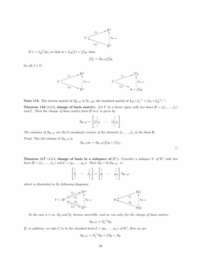
If f = L−1B (x), so that x = LB(f) = [f ]B, then
[T (f)]B = B[f ]B
for all f ∈ V :
VT−−−−−−−−−→ V
LB
y LB
yRn B−−−−−−−−−→ Rn
fT−−−−−−−−−→ T (f)
LB
y LB
yx = [f ]B
B−−−−−−−−−→ [T (f)]B
Theorem 113 (4.3.2, B-matrix of a linear transformation). Let V be a linear space with basis B =(f1, . . . , fn), and let T : V → V be a linear transformation. Then the B-matrix of T is given by
B =
| |[T (f1)]B · · · [T (fn)]B| |
.The columns of B are the B-coordinate vectors of the transforms of the elements f1, . . . , fn in the basis B.
Proof. The ith column of B isBei = B[fi]B = [T (fi)]B.
Definition 114 (4.3.3). Let V be an n-dimensional linear space with bases B and C, and let T : V → V bea linear transformation. The change of basis matrix from B to C, denoted by SB→C , is defined to be thestandard matrix of the linear transformation LC L−1B : Rn → Rn, so that
SB→Cx = LC(L−1B (x))
for all x ∈ Rn:
27
Rn
V
LC44jjjjjjjjjjjj
Rn
SB→C
OO
L−1B
jjTTTTTTTTTTTT
If f = L−1B (x), so that x = LB(f) = [f ]B, then
[f ]C = SB→C [f ]B
for all f ∈ V :
Rn
V
LC44jjjjjjjjjjjj
LB **TTTTTTTTTTTT
Rn
SB→C
OO
[f ]C
f
LC44jjjjjjjjjjjj
LB **TTTTTTTTTT
x = [f ]B
SB→C
OO
Note 115. The inverse matrix of SB→C is SC→B, the standard matrix of LB L−1C = (LC L−1B )−1.
Theorem 116 (4.3.3, change of basis matrix). Let V be a linear space with two bases B = (f1, . . . , fn)and C. Then the change of basis matrix from B to C is given by
SB→C =
| |[f1]C · · · [fn]C| |
.The columns of SB→C are the C-coordinate vectors of the elements f1, . . . , fn in the basis B.
Proof. The ith column of SB→C isSB→Cei = SB→C [fi]B = [fi]C .
Theorem 117 (4.3.4, change of basis in a subspace of Rn). Consider a subspace V of Rn with twobases B = (f1, . . . , fm) and C = (g1, . . . , gm). Then SB = SCSB→C, or | |
f1 · · · fm| |
=
| |g1 · · · gm| |
SB→C ,which is illustrated in the following diagrams:
Rm
SCttjjjjjjjjj
V ⊂ Rn
LC44jjjjjjjjj
LB **TTTTTTTTT
Rm
SB→C
OOSB
jjTTTTTTTTT
[x]C
SCttjjjjjjjjjjjj
x
[x]B
SB→C
OOSB
jjTTTTTTTTTTTT
In the case n = m, SB and SC become invertible, and we can solve for the change of basis matrix:
SB→C = S−1C SB.
If, in addition, we take C to be the standard basis E = (e1, . . . , en) of Rn, then we get
SB→E = S−1E SB = ISB = SB.
28
Proof. By definition, SB→Cx = LC(L−1B (x)) for any x ∈ Rm, and we can apply L−1C to both sides to obtain
L−1C (SB→Cx) = L−1B (x).
By Note 99, we can rewrite this as SCSB→Cx = SBx. Since this holds for any x ∈ Rm, we conclude thatSCSB→C = SB.
When n = m, SB and SC are n× n matrices whose columns form bases, so they are invertible.
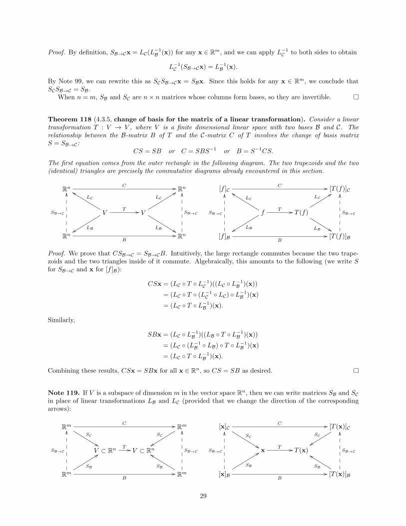
Theorem 118 (4.3.5, change of basis for the matrix of a linear transformation). Consider a lineartransformation T : V → V , where V is a finite dimensional linear space with two bases B and C. Therelationship between the B-matrix B of T and the C-matrix C of T involves the change of basis matrixS = SB→C:
CS = SB or C = SBS−1 or B = S−1CS.
The first equation comes from the outer rectangle in the following diagram. The two trapezoids and the two(identical) triangles are precisely the commutative diagrams already encountered in this section.
Rn C // Rn
VT //
LC
eeKKKKKKKKKK
LByyssssssssss V
LC
99ssssssssss
LB %%KKKKKKKKKK
Rn
SB→C
OO
B// Rn
SB→C
OO
[f ]CC // [T (f)]C
fT //
LC
eeKKKKKKKKKK
LByyssssssssss T (f)
LC99ssssssss
LB %%KKKKKKKK
[f ]B
SB→C
OO
B// [T (f)]B
SB→C
OO
Proof. We prove that CSB→C = SB→CB. Intuitively, the large rectangle commutes because the two trape-zoids and the two triangles inside of it commute. Algebraically, this amounts to the following (we write Sfor SB→C and x for [f ]B):
CSx = (LC T L−1C )((LC L−1B )(x))
= (LC T (L−1C LC) L−1B )(x)
= (LC T L−1B )(x).
Similarly,
SBx = (LC L−1B )((LB T L−1B )(x))
= (LC (L−1B LB) T L−1B )(x)
= (LC T L−1B )(x).
Combining these results, CSx = SBx for all x ∈ Rn, so CS = SB as desired.
Note 119. If V is a subspace of dimension m in the vector space Rn, then we can write matrices SB and SCin place of linear transformations LB and LC (provided that we change the direction of the correspondingarrows):
Rm C //
SC
%%KKKKKKKKK RmSC
yysssssssss
V ⊂ Rn T // V ⊂ Rn
Rm
SB→C
OO
B//
SB
99sssssssssRm
SB→C
OOSB
eeKKKKKKKKK
[x]CC //
SC
%%KKKKKKKKKK [T (x)]CSC
yyssssssss
xT // T (x)
[x]B
SB→C
OO
B//
SB
99ssssssssss[T (x)]B
SB→C
OOSB
eeKKKKKKKK
29
Finally, if V = Rn and we take C to be the standard basis E = (e1, . . . , en) of Rn, then the E-matrix of Tequals the standard matrix A of T , SE = I, SB→E = SB, and the picture simplifies to the following, wherethe outer rectangle gives the familiar formula ASB = SBB from Theorem 87:
Rn A // Rn
V = Rn T //
KKKKKKKKKK
KKKKKKKKKK
V = Rn
ssssssssss
ssssssssss
Rn
SB
OO
B//
SB
99ssssssssssRn
SB
OOSB
eeKKKKKKKKKK
[x]EA // [T (x)]E
xT //
KKKKKKKKKK
KKKKKKKKKKT (x)
ssssssss
ssssssss
[x]B
SB
OO
B//
SB
99ssssssssss[T (x)]B
SB
OOSB
eeKKKKKKKK
30
5 Orthogonality and Least Squares
5.1 Orthogonal Projections and Orthonormal Bases
Definition 120 (5.1.1).
• Two vectors v,w ∈ Rn are called perpendicular or orthogonal if v ·w = 0.
• A vector x ∈ Rn is orthogonal to a subspace V ⊂ Rn if x is orthogonal to all vectors v ∈ V .
Theorem 121. A vector x ∈ Rn is orthogonal to a subspace V ⊂ Rn with basis v1, . . . ,vm if and onlyif x is orthogonal to all of the basis vectors v1, . . . ,vm.
Proof. If x is orthogonal to V , then x is orthogonal to v1, . . . ,vm by definition.Conversely, if x is orthogonal to v1, . . . ,vm, then any v ∈ V can be written as a linear combination
v = c1v1 + · · ·+ cmvm of basis vectors, from which it follows that
x · v = x · (c1v1 + · · ·+ cmvm)
= x · (c1v1) + · · ·+ x · (cmvm)
= c1(x · v1) + · · ·+ cm(x · vm)
= c1(0) + · · ·+ cm(0)
= 0,
so x is orthogonal to v.
Definition 122 (5.1.1).
• The length (or magnitude or norm) of a vector v ∈ Rn is ||v|| =√
v · v.
• A vector u ∈ Rn is called a unit vector if its length is 1 (i.e., ||u|| = 1 or u · u = 1).
Theorem 123.
• For any vectors v,w ∈ Rn and scalar k ∈ R,
k(v ·w) = (kv) ·w = v · (kw) and ||kv|| = |k| ||v|| .
• If v 6= 0, then the vector u = 1||v||v is a unit vector in the same direction as v, called the normalization
of v.
Proof.
• We compute
(kv) ·w =
n∑i=1
(kv)iwi =
n∑i=1
kviwi = k
n∑i=1
viwi = k(v ·w),
v · (kw) =
n∑i=1
vi(kw)i =
n∑i=1
vikwi = k
n∑i=1
viwi = k(v ·w),
which proves the first claim. We then use the definition of length to obtain
||kv|| =√
(kv) · (kv) =√k2(v · v) =
√k2√
v · v = |k| ||v|| .
31
• To prove that the normalization u is a unit vector, we compute its length:
||u|| =∣∣∣∣∣∣∣∣ 1
||v||v
∣∣∣∣∣∣∣∣ =
∣∣∣∣ 1
||v||
∣∣∣∣ ||v|| = 1
||v||||v|| = 1.
Definition 124 (5.1.2). The vectors u1, . . . ,um ∈ Rn are called orthonormal if they are all unit vectorsand all orthogonal to each other:
ui · uj =
1 if i = j
0 if i 6= j.
Note 125. The standard basis vectors e1, . . . , en of Rn are orthonormal.
Since all of the dot products are 0 except for ui · ui = 1, we have ci = 0. This is true for all i = 1, 2, . . . ,m,so u1, . . . ,um are linearly independent.
Theorem 127 (5.1.4, orthogonal projection). For any vector x ∈ Rn and any subspace V ⊂ Rn, we canwrite
x = x‖ + x⊥
for some x‖ in V and x⊥ perpendicular to V , and this representation is unique. The vector projV (x) = x‖
is called the orthogonal projection of x onto V and is given by the formula
projV (x) = x‖ = (u1 · x)u1 + · · ·+ (um · x)um
for all x ∈ Rn, where (u1, . . . ,um) is any orthonormal basis of V . The resulting orthogonal projectiontransformation projV : Rn → Rn is linear.
Proof. Any potential projV (x) = x‖ ∈ V can be written as a linear combination
Thus the unique solution has ci = ui · x for i = 1, . . . ,m, which means that
x‖ = (u1 · x)u1 + · · ·+ (um · x)um
andx⊥ = x− (u1 · x)u1 − · · · − (um · x)um.
For linearity, take x,y ∈ Rn and k ∈ R. Then
x + y = (x‖ + x⊥) + (y‖ + y⊥) = (x‖ + y‖) + (x⊥ + y⊥),
with x‖ + y‖ in V and x⊥ + y⊥ orthogonal to V , so
projV (x + y) = x‖ + y‖ = projV (x) + projV (y).
Similarly,kx = k(x‖ + x⊥) = kx‖ + kx⊥,
with kx‖ in V and kx⊥ orthogonal to V , so
projV (kx) = kx‖ = k projV (x).
Note 128. The orthogonal projection of x onto a subspace V ⊂ Rn is obtained by summing the orthogonalprojections (ui · x)ui of x onto the lines spanned by the orthonormal basis vectors u1, . . . ,um of V .
Theorem 129 (5.1.6, coordinates via orthogonal projection). For any orthonormal basis B =(u1, . . . ,un) of Rn,
x = (u1 · x)u1 + · · ·+ (un · x)un
for all x ∈ Rn, so the B-coordinate vector of x is given by
[x]B =
u1 · x...
un · x
.Proof. If V = Rn in Theorem 127, then clearly x = x + 0 is a decomposition of x with x in V and 0orthogonal to V . Thus
x = x‖ = projV (x) = (u1 · x)u1 + · · ·+ (un · x)un.
Definition 130 (5.1.7). The orthogonal complement V ⊥ of a subspace V ⊂ Rn is the set of all vectorsx ∈ Rn which are orthogonal to all vectors in v ∈ V :
V ⊥ = x ∈ Rn : v · x = 0 for all v ∈ V .
Theorem 131. For a subspace V ⊂ Rn, the orthogonal complement V ⊥ is the kernel of projV . The imageof projV is V itself.
Proof. Note that x ∈ V ⊥ if and only if x⊥ = x, i.e. projV (x) = x‖ = 0.Any vector in the image of projV is contained in V by definition. Conversely, for any v ∈ V , projV (v) = v,
so v is in the image of projV .
33
Theorem 132 (5.1.8, properties of the orthogonal complement). Let V be a subspace of Rn.
a) V ⊥ is a subspace of Rn.
b) V ∩ V ⊥ = 0
c) dim(V ) + dim(V ⊥) = n
d) (V ⊥)⊥ = V
Proof.
a) By the preceding theorem, V ⊥ is the kernel of the linear transformation projV : Rn → Rn and istherefore a subspace of the domain Rn.
b) Clearly 0 is contained in both V and V ⊥. Any vector x in both V and V ⊥ is orthogonal to itself, so
that x · x = ||x||2 = 0 and thus x = 0.
c) Applying the Rank-Nullity Theorem to the linear transformation projV : Rn → Rn, we have
Multiplying each side by ||y||, we get||x|| ||y|| ≥ |x · y| .
Definition 136 (5.1.12). By the Cauchy-Schwarz inequality,∣∣∣ x·y||x||||y||
∣∣∣ = |x·y|||x||||y|| ≤ 1, so we may define the
angle between two nonzero vectors x,y ∈ Rn to be
θ = arccosx · y||x|| ||y||
.
With this definition, we have the formula
x · y = ||x|| ||y|| cos θ
for the dot product in terms of the lengths of two vectors and the angle between them.
5.2 Gram-Schmidt Process and QR Factorization
Theorem 137 (5.2.1). For a basis v1, . . . ,vm of a subspace V ⊂ Rn, define subspaces
Vj = span(v1, . . . ,vj) ⊂ V
for j = 0, 1, . . . ,m. Note that V0 = span ∅ = 0 and Vm = V .Let v⊥j be the component of vj perpendicular to the span Vj−1 of the preceding basis vectors:
v⊥j = vj − v‖j = vj − projVj−1
(vj).
We can normalize the v⊥j to obtain unit vectors:
uj =1∣∣∣∣v⊥j ∣∣∣∣v⊥j .
Then u1, . . . ,um form an orthonormal basis of V .
Proof. In order to define uj , we must ensure that v⊥j 6= 0. This holds because vj is not redundant in thelist v1, . . . ,vj , and thus is not contained in Vj−1.
By definition, the vj are all orthogonal to each other. Thus the uj are too, since
ui · uj =
(1∣∣∣∣v⊥i ∣∣∣∣v⊥i
)·
(1∣∣∣∣v⊥j ∣∣∣∣v⊥j
)=
1∣∣∣∣v⊥i ∣∣∣∣ ∣∣∣∣v⊥j ∣∣∣∣ (vi · vj) = 0.
Since u1, . . . ,um ∈ V are orthogonal unit vectors, they are linearly independent. Since dim(V ) = m, thesevectors form an (orthonormal) basis for V .
35
Procedure 138 (5.2.1, Gram-Schmidt orthogonalization). We compute the orthonormal basis u1, . . . ,umof the preceding theorem by performing the following steps for j = 0, 1, . . . ,m.
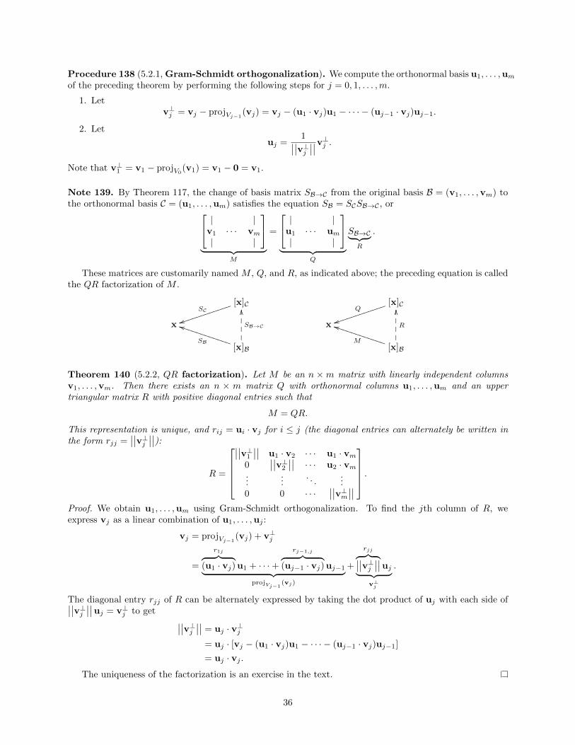
Note 139. By Theorem 117, the change of basis matrix SB→C from the original basis B = (v1, . . . ,vm) tothe orthonormal basis C = (u1, . . . ,um) satisfies the equation SB = SCSB→C , or | |
v1 · · · vm| |
︸ ︷︷ ︸
M
=
| |u1 · · · um| |
︸ ︷︷ ︸
Q
SB→C︸ ︷︷ ︸R
.
These matrices are customarily named M , Q, and R, as indicated above; the preceding equation is calledthe QR factorization of M .
[x]CSC
ttjjjjjjjjjjjj
x
[x]B
SB→C
OO
SB
jjTTTTTTTTTTTT
[x]CQ
ttjjjjjjjjjjjj
x
[x]B
R
OO
M
jjTTTTTTTTTTTT
Theorem 140 (5.2.2, QR factorization). Let M be an n ×m matrix with linearly independent columnsv1, . . . ,vm. Then there exists an n × m matrix Q with orthonormal columns u1, . . . ,um and an uppertriangular matrix R with positive diagonal entries such that
M = QR.
This representation is unique, and rij = ui · vj for i ≤ j (the diagonal entries can alternately be written inthe form rjj =
∣∣∣∣v⊥j ∣∣∣∣):
R =
∣∣∣∣v⊥1 ∣∣∣∣ u1 · v2 · · · u1 · vm
0∣∣∣∣v⊥2 ∣∣∣∣ · · · u2 · vm
......
. . ....
0 0 · · ·∣∣∣∣v⊥m∣∣∣∣
.Proof. We obtain u1, . . . ,um using Gram-Schmidt orthogonalization. To find the jth column of R, weexpress vj as a linear combination of u1, . . . ,uj :
vj = projVj−1(vj) + v⊥j
=
r1j︷ ︸︸ ︷(u1 · vj) u1 + · · ·+
rj−1,j︷ ︸︸ ︷(uj−1 · vj) uj−1︸ ︷︷ ︸
projVj−1(vj)
+
rjj︷ ︸︸ ︷∣∣∣∣v⊥j ∣∣∣∣uj︸ ︷︷ ︸v⊥j
.
The diagonal entry rjj of R can be alternately expressed by taking the dot product of uj with each side of∣∣∣∣v⊥j ∣∣∣∣uj = v⊥j to get ∣∣∣∣v⊥j ∣∣∣∣ = uj · v⊥j= uj · [vj − (u1 · vj)u1 − · · · − (uj−1 · vj)uj−1]
= uj · vj .
The uniqueness of the factorization is an exercise in the text.
36
5.3 Orthogonal Transformations and Orthogonal Matrices
Definition 141 (5.3.1). A linear transformation T : Rn → Rn is called orthogonal if it preserves thelength of vectors:
||T (x)|| = ||x|| , for all x ∈ Rn.
If T (x) = Ax is an orthogonal transformation, we say that A is an orthogonal matrix.
Theorem 142 (5.3.2, orthogonal transformations preserve orthogonality). Let T : Rn → Rn be anorthogonal linear transformation. If v,w ∈ Rn are orthogonal, then so are T (v), T (w).
Proof. We compute:
||T (v) + T (w)||2 = ||T (v + w)||2
= ||v + w||2
= ||v||2 + ||w||2
= ||T (v)||2 + ||T (w)||2 ,
so T (v) is orthogonal to T (w) by the Pythagorean Theorem.
Note 143. In fact, orthogonal transformations preserve all angles, not just right angles: the angle betweentwo nonzero vectors v,w ∈ Rn equals the angle between T (v), T (w). This is a homework problem.
Theorem 144 (orthogonal transformations preserve the dot product). A linear transformationT : Rn → Rn is orthogonal if and only if T preserves the dot product:
v ·w = T (v) · T (w) for all v,w ∈ Rn.
Proof. Suppose T is orthogonal. Then T preserves the length of v + w, so
||T (v + w)||2 = ||v + w||2
(T (v) + T (w)) · (T (v) + T (w)) = (v + w) · (v + w)
T (v) · T (v) + 2T (v) · T (w) + T (w) · T (w) = v · v + 2v ·w + w ·w
where we have used that ||T (v)|| = ||v|| and ||T (w)|| = ||w||.Conversely, suppose T preserves the dot product. Then
||T (v)||2 = T (v) · T (v) = v · v = ||v||2 ,
so ||T (v)|| = ||v||, and T is orthogonal.
Theorem 145 (5.3.3, orthogonal matrices and orthonormal bases). An n×n matrix A is orthogonalif and only if its columns form an orthonormal basis of Rn.
Proof. Define T (x) = Ax and recall that
A =
| |T (e1) · · · T (en)| |
.37
SupposeA, and hence T , are orthogonal. Because e1, . . . , en are orthonormal, their images T (e1), . . . , T (en)are also orthonormal, since T preserves length and orthogonality. By Theorem 126, T (e1), . . . , T (en) arelinearly independent. Since dim(Rn) = n, the columns T (e1), . . . , T (en) of A form an (orthonormal) basisof Rn.
Conversely, suppose T (e1), . . . , T (en) form an orthonormal basis of Rn. Then for any x = x1e1 + · · · +xnen ∈ Rn,
where the second equals sign follows from the Pythagorean Theorem. Then ||T (x)|| = ||x|| and T and A areorthogonal.
Theorem 146 (5.3.4, products and inverses of orthogonal matrices).
a) The product AB of two orthogonal n× n matrices A and B is orthogonal.
b) The inverse A−1 of an orthogonal n× n matrix A is orthogonal.
Proof.
a) The linear transformation T (x) = (AB)x is orthogonal because
||T (x)|| = ||A(Bx)|| = ||Bx|| = ||x|| .
b) The linear transformation T (x) = A−1x is orthogonal because
||T (x)|| =∣∣∣∣A−1x∣∣∣∣ =
∣∣∣∣A(A−1x)∣∣∣∣ = ||Ix|| = ||x|| .
Definition 147 (5.3.5). For an m × n matrix A, the transpose AT of A is the n ×m matrix whose ijthentry is the jith entry of A:
[AT ]ij = Aji.
The rows of A become the columns of AT , and the columns of A become the rows of AT .A square matrix A is symmetric if AT = A and skew-symmetric if AT = −A.
Note 148 (5.3.6). If v and w are two (column) vectors in Rn, then
v ·w = vTw.
(Here we choose to ignore the difference between a scalar a and the 1× 1 matrix[a]).
Theorem 149 (5.3.7, transpose criterion for orthogonal matrices). An n× n matrix A is orthogonalif and only if ATA = In or, equivalently, if A has inverse A−1 = AT .
.This product equals In if and only if the columns of A are orthonormal, which is equivalent to A being anorthogonal matrix.
If A is orthogonal, it is also invertible, since its columns form an (orthonormal) basis of Rn. ThusATA = In is equivalent to A−1 = AT by simple matrix algebra.
Theorem 150 (5.3.8, summary: orthogonal matrices). For an n×n matrix A, the following statementsare equivalent:
1. A is an orthogonal matrix.
2. ||Ax|| = ||x|| for all x ∈ Rn.
3. The columns of A form an orthonormal basis of Rn.
4. ATA = In.
5. A−1 = AT .
Proof. See Definition 141 and Theorems 145 and 149.
Theorem 151 (5.3.9, properties of the transpose).
a) If A is an n× p matrix and B a p×m matrix (so that AB is defined), then
(AB)T = BTAT .
b) If an n× n matrix A is invertible, then so is AT , and
(AT )−1 = (A−1)T .
c) For any matrix A,rank(A) = rank(AT ).
Proof.
a) We check that the ijth entries of the two matrices are equal:
[(AB)T ]ij = [AB]ji = (jth row of A) · (ith column of B),
[BTAT ]ij = (ith row of BT ) · (jth column of AT ) = (ith column of B) · (jth row of A).
b) Taking the transpose of both sides of AA−1 = I and using part (a), we get
(AA−1)T = (A−1)TAT = I.
Similarly, A−1A = I implies(A−1A)T = AT (A−1)T = I.
We conclude that the inverse of AT is (A−1)T .
39
c) Suppose A has n columns. Since the vectors in the kernel of A are precisely those vectors in Rn whichare orthogonal to all of the rows of A, and hence to the span of the rows of A,
span(rows of A) = (kerA)⊥.
By the Rank-Nullity Theorem, together with its corollary in Theorem 132 part (c),
rank(AT ) = dim(imAT )
= dim(span(columns of AT ))
= dim(span(rows of A))
= dim((kerA)⊥)
= n− dim(kerA)
= dim(imA)
= rank(A).
Theorem 152 (invertibility criteria involving rows). For an n × n matrix A =
− w1 −...
− wn −
, the
following are equivalent:
1. A is invertible,
2. w1, . . . ,wn span Rn,
3. w1, . . . ,wn are linearly independent,
4. w1, . . . ,wn form a basis of Rn.
Proof. By the preceding theorem, A is invertible if and only if AT is invertible. Statements 2-4 are just thelast three invertibility criteria in Theorem 80 applied to AT , since the columns of AT are the rows of A.
Theorem 153 (column-row definition of matrix multiplication). Given matrices
A =
| |v1 · · · vm| |
and B =
− w1 −...
− wm −
,with v1, . . . ,vm,w1, . . . ,wm ∈ Rn, think of the vi as n× 1 matrices and the wi as 1×n matrices. Then theproduct of A and B can be computed as a sum of m n× n matrices:
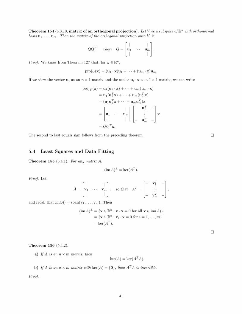
Theorem 154 (5.3.10, matrix of an orthogonal projection). Let V be a subspace of Rn with orthonormalbasis u1, . . . ,um. Then the matrix of the orthogonal projection onto V is
QQT , where Q =
| |u1 · · · um| |
.Proof. We know from Theorem 127 that, for x ∈ Rn,
projV (x) = (u1 · x)u1 + · · ·+ (um · x)um.
If we view the vector ui as an n× 1 matrix and the scalar ui · x as a 1× 1 matrix, we can write
projV (x) = u1(u1 · x) + · · ·+ um(um · x)
= u1(uT1 x) + · · ·+ um(uTmx)
= (u1uT1 x + · · ·+ umuTm)x
=
| |u1 · · · um| |
− uT1 −
...− uTm −
x
= QQTx.
The second to last equals sign follows from the preceding theorem.
5.4 Least Squares and Data Fitting
Theorem 155 (5.4.1). For any matrix A,
(imA)⊥ = ker(AT ).
Proof. Let
A =
| |v1 · · · vm| |
, so that AT =
− vT1 −...
− vTm −
,and recall that im(A) = span(v1, . . . ,vm). Then
(imA)⊥ = x ∈ Rn : v · x = 0 for all v ∈ im(A)= x ∈ Rn : vi · x = 0 for i = 1, . . . ,m= ker(AT ).
Theorem 156 (5.4.2).
a) If A is an n×m matrix, thenker(A) = ker(ATA).
b) If A is an n×m matrix with ker(A) = 0, then ATA is invertible.
Proof.
41
a) If Ax = 0, then ATAx = 0, so ker(A) ⊂ ker(ATA).
Conversely, if ATAx = 0, then Ax ∈ ker(A) and Ax ∈ im(AT ) = (kerA)⊥, so Ax = 0 by Theorem132 part (b). Thus ker(ATA) ⊂ ker(A).
b) Since ATA is an m×m matrix and, by part (a), ker(ATA) = 0, ATA is invertible by Theorem 47.
Theorem 157 (5.4.3, alternative characterization of orthogonal projection). Given a vector x ∈ Rnand a subspace V ⊂ Rn, the orthogonal projection projV (x) is the vector in V closest to x, i.e.,
||x− projV (x)|| < ||x− v||
for all v ∈ V not equal to projV (x).
Proof. Note that x− projV (x) = x⊥ ∈ V ⊥, while projV (x)− v ∈ V , so the two vectors are orthogonal. Wecan therefore apply the Pythagorean Theorem:
This implies that ||x− projV (x)||2 < ||x− v||2 unless ||projV (x)− v||2 = 0, i.e. projV (x) = v.
Definition 158 (5.4.4). Let A be an n × m matrix. Then a vector x∗ ∈ Rm is called a least-squaressolution of the system Ax = b if the distance between Ax∗ and b is as small as possible:
||b−Ax∗|| ≤ ||b−Ax|| for all x ∈ Rm.
Note 159. The vector x∗ is called a “least-squares solution” because it minimizes the sum of the squaresof the components of the “error” vector b− Ax. If the system Ax = b is consistent, then the least-squaressolutions x∗ are just the exact solutions, so that the error b−Ax∗ = 0.
Theorem 160 (5.4.5, the normal equation). The least-squares solutions of the system
Ax = b
are the exact solutions of the (consistent) system
ATAx = ATb,
which is called the normal equation of Ax = b.
Proof. We have the following chain of equivalent statements:
The vector x∗ is a least-squares solution of the system Ax = b
⇐⇒ ||b−Ax∗|| ≤ ||b−Ax|| for all x ∈ Rm
⇐⇒ Ax∗ = proj(imA)(b)
⇐⇒ b−Ax∗ ∈ (imA)⊥ = ker(AT )
⇐⇒ AT (b−Ax∗) = 0
⇐⇒ ATAx∗ = ATb.
42
Theorem 161 (5.4.6, unique least-squares solution). If ker(A) = 0, then the linear system Ax = b hasthe unique least-squares solution
x∗ = (ATA)−1ATb.
Proof. By Theorem 156 part (b), the matrix ATA is invertible. Multiplying each side of the normal equationon the left by (ATA)−1, we obtain the result.
Theorem 162 (5.4.7, matrix of an orthogonal projection). Let v1, . . . ,vm be any basis of a subspaceV ⊂ Rn, and set
A =
| |v1 · · · vm| |
.Then the matrix of the orthogonal projection onto V is
A(ATA)−1AT .
Proof. Let b be any vector in Rn. If x∗ is a least-squares solution of Ax = b, then Ax∗ is the projectiononto V = im(A) of b. Since the columns of A are linearly independent, ker(A) = 0, so we have the uniqueleast-squares solution
x∗ = (ATA)−1ATb.
Multiplying each side by A on the left, we get
projV (b) = Ax∗ = A(ATA)−1ATb.
Note 163. If v1, . . . ,vm form an orthonormal basis, then ATA = Im and the formula for the matrix of anorthogonal projection simplifies to AAT , as in Theorem 154.
5.5 Inner Product Spaces
Definition 164 (5.5.1). An inner product on a linear space V is a rule that assigns a scalar, denoted〈f, g〉, to any pair f, g of elements of V , such that the following properties hold for all f, g, h ∈ V and allc ∈ R:
3. preserves scalar multiplication: 〈cf, g〉 = c 〈f, g〉
4. positive definiteness: 〈f, f〉 > 0 for all nonzero f ∈ V .
A linear space endowed with an inner product is called an inner product space.
Note 165. Properties 2 and 3 state that, for a fixed g ∈ V , the transformation T : V → R given byT (f) = 〈f, g〉 is linear.
Definition 166. We list some examples of inner product spaces:
43
• Let C[a, b] be the linear space of continuous functions from the interval [a, b] to R. Then
〈f, g〉 =
∫ b
a
f(t)g(t) dt
defines an inner product on C[a, b].
• Let `2 be the linear space of all “square-summable” infinite sequences, i.e., sequences
x = (x0, x1, x2, . . . , xn, . . .),
such that∑∞i=0 x
2i = x20 + x21 + · · · converges. Then
〈x,y〉 =
∞∑i=0
xiyi = x0y0 + x1y1 + · · ·
defines an inner product on `2.
• The trace of a square matrix A, denoted tr(A), is the sum of its diagonal entries. An inner producton the linear space Rn×m of all n×m matrices is given by
〈A,B〉 = tr(ATB).
Definition 167 (5.5.2).
• The norm (or magnitude) of an element f of an inner product space is
||f || =√〈f, f〉.
• Two elements f, g of an inner product space are called orthogonal (or perpendicular) if
〈f, g〉 = 0.
• The distance between two elements of an inner product space is defined to be the norm of theirdifference:
dist(f, g) = ||f − g|| .
• The angle θ between two elements f, g of an inner product space is defined by the formula
θ = cos−1(〈f, g〉||f || ||g||
).
Theorem 168 (5.5.3, orthogonal projection). If V is an inner product space with finite dimensionalsubspace W , then the orthogonal projection projW (f) of an element f ∈ V onto W is defined to be theunique element of W such that f − projW (f) is orthogonal to W . Alternately, projW (f) is the element ofW which minimizes
dist(f, projW (f)) = ||f − projW (F )|| .
If g1, . . . , gm is an orthonormal basis of W , then
projW (f) = 〈g1, f〉 g1 + · · ·+ 〈gm, f〉 gm
for all f ∈ V .
44
Definition 169. Consider the inner product
〈f, g〉 =1
π
∫ π
−πf(t)g(t) dt
on the linear space C[−π, π] of continuous functions on the interval [−π, π]. For each positive integer n,define the subspace Tn of C[−π, π] to be
−πsin(pt) sin(mt) dt = 0, for distinct integers p,m,
〈cos(pt), cos(mt)〉 =1
π
∫ π
−πcos(pt) cos(mt) dt = 0, for distinct integers p,m.
(Note that 1 = cos(0t).) Thus the functions 1, sin(t), cos(t), sin(2t), cos(2t), . . . , sin(nt), cos(nt) are orthogo-nal to each other, and hence linearly independent. Since they clearly span Tn, they form a basis for Tn.
To obtain an orthonormal basis for Tn, we normalize the vectors. Since
||1|| =
√1
π
∫ π
−π1 dt =
√2,
||sin(mt)|| =
√1
π
∫ π
−πsin2(mt) dt = 1,
||cos(mt)|| =
√1
π
∫ π
−πcos2(mt) dt = 1,
we need only replace the function 1 by 1/ ||1|| = 1/√
2.
Theorem 171 (5.5.5, Fourier coefficients). The best approximation (in the “continuous least-squares”sense) of f ∈ C[−π, π] by function in the subspace Tn is
Proof. The first equality is proven using advanced calculus. The second one follows from the first, since
||f − fn||2 + ||fn||2 = ||f ||2
by the Pythagorean Theorem. For the final equality, we use the preceding note to substitute for ||fn||2 in
limn→∞
||fn||2 = ||f ||2 .
Note 174. Applying the final equation of Theorem 173 to the function f(t) = t in C[−π, π], we obtain
4 +4
4+
4
9+ · · ·+ 4
n2+ · · · = ||t||2 =
1
π
∫ π
−πt2 dt =
2
3π2,
or,∞∑n=1
1
n2= 1 +
4
4+
4
9+
4
16+ · · · = π2
6, i.e., π =
√√√√6
∞∑n=1
1
n2.
46
6 Determinants
6.1 Introduction to Determinants
Note 175. A 2× 2 matrix
A =
[a bc d
]is invertible if and only if det(A) = ad − bc 6= 0. The geometric reason for this is that (the absolute valueof) the determinant measures the area of the parallelogram spanned by the columns of A. In particular,(
area of parallelogram spanned by
[ac
]and
[bd
])=
∣∣∣∣∣∣∣∣∣∣∣∣ac
0
×bd
0
∣∣∣∣∣∣∣∣∣∣∣∣ =
∣∣∣∣∣∣∣∣∣∣∣∣ 0
0ad− bc
∣∣∣∣∣∣∣∣∣∣∣∣ = |ad− bc| = |det(A)| .
Thus, we have the following chain of equivalent statements:
A is invertible ⇐⇒ the columns
[ac
]and
[bd
]of A are linearly independent
⇐⇒ the area of the parallelogram spanned by
[ac
]and
[bd
]is nonzero
⇐⇒ det(A) = ad− bc 6= 0.
Definition 176 (6.1.1). Consider the 3× 3 matrix
A =
| | |u v w| | |
=
u1 v1 w1
u2 v2 w2
u3 v3 w3
.We define the determinant of A to be the volume of the parallelepiped spanned by the column vectorsu,v,w of A, namely
det(A) = u · (v ×w),
also known as the “triple product” of u,v,w. Then, as in the 2× 2 case,
A is invertible ⇐⇒ the columns u,v,w of A are linearly independent
⇐⇒ the volume of the parallelepiped spanned by u,v,w is nonzero
Note 177. In the final expression above for det(A), note that each term contains exactly one entry fromeach row and each column of A. We have written the terms so that u, v, w always occur in the same order;only the indices change. In fact, the indices occur once in each of the 3! = 6 possible permutations.
The sign on each term in the determinant formula is determined by how many pairs of indices are “out oforder,” or “inverted,” in the corresponding permutation of the numbers 1, 2, 3. If the number of “inversions”is even, then the sign of the term is positive, and if odd, then negative.
For example, in the permutation 3, 1, 2, the pair of numbers 1, 3 is inverted, as is the pair 2, 3. In termof the entries of the matrix A, this can be visualized by noting that v1 and w2 are both above and to theright of u3. Since the number of inversions is even, the term u3v1w2 occurs with a positive sign.
Armed with this insight, we can define the determinant of a general n× n matrix.
47
Definition 178 (6.1.3).
• A pattern in an n × n matrix A is a choice of n entries of the matrix so that one entry is chosen ineach row and in each column of A. The product of the entries in a pattern P is denoted prodP .
• Two entries in a pattern are said to be inverted if one of them is above and to the right of the otherin the matrix.
• The signature of a pattern P is
sgnP = (−1)number of inversions in P .
• The determinant of A is then defined to be
detA =∑
(sgnP )(prodP ),
where the sum is taken over all n! patterns P in the matrix.
Note 179. If we separate the positive terms from the negative terms, we can write:
detA =
∑patterns P with aneven # of inversions
prodP
− ∑
patterns P with anodd # of inversions
prodP
.
Note 180. For a 2× 2 matrix
A =
[a bc d
],
there are two patterns, with products ad and bc. They have 0 and 1 inversions, respectively, so detA =(1−)0ad+ (−1)1bc = ad− bc, as expected.
Theorem 181 (6.1.4, determinant of a triangular matrix). The determinant of an upper or lowertriangular matrix is the product of the diagonal entries of the matrix. In particular, the determinant of adiagonal matrix is the product of its diagonal entries.
Proof. For an upper triangular n× n matrix A, a pattern with nonzero product must contain a11, and thusa22, . . . , and finally ann, so there is only one pattern with potentially nonzero product. This diagonalpattern has no inversions, so its product is equal to detA.
The proof for a lower triangular matrix is analogous, and a diagonal matrix is a special case.
6.2 Properties of the Determinant
Theorem 182 (6.2.1, determinant of the transpose). For any square matrix A,
det(AT ) = detA.
Proof. Every pattern in A corresponds to a (transposed) pattern in AT with the same product and numberof inversions. Thus the determinants are equal.
48
Theorem 183 (6.2.2, linearity of the determinant in each row and column). Let w1, . . . ,wi−1,wi+1, . . . ,wn ∈ Rn be fixed row vectors. Then the function T : R1×n → R given by
T (x) = det
− w1 −...
− vi−1 −− x −− vi+1 −
...− vn −
is a linear transformation. We say that the determinant is linear in the ith row.
Similarly, let v1, . . . ,vi−1, vi+1, . . . ,vn ∈ Rn be fixed column vectors. Then the function T : Rn×1 → Rgiven by
T (x) = det
| | | | |v1 · · · vi−1 x vi+1 · · · vn| | | | |
is a linear transformation. We say that the determinant is linear in the ith column.
Proof. The product prodP of a pattern P is linear in each row and column because it contains exactly onefactor from each row and one from each column. Since the determinant is a linear combination of patternproducts, it is linear in each row and column as well.
Note 184. The preceding theorem states that T (x+y) = T (x) +T (y) and T (kx) = kT (x), or, for linearityin a row,
det
− v1 −...
− x + y −...
− vn −
= det
− v1 −...
− x −...
− vn −
+
− v1 −...
− x −...
− vn −
and
det
− v1 −...
− kx −...
− vn −
= k det
− v1 −...
− x −...
− vn −
.
Theorem 185 (6.2.3, elementary row operations and determinants). The elementary row operationshave the following effects on the determinant of a matrix.
a) If B is obtained from A by a row swap, then
detB = −detA.
b) If B is obtained from A by dividing a row of A by a scalar k, then
detB =1
kdetA.
c) If B is obtained from A by adding a multiple of a row of A to another row, then
detB = detA.
49
Proof.
a) Row swap: Each pattern P in A corresponds to a pattern Pswap in B involving the same numbers.If adjacent rows are swapped, then the number of inversions changes by exactly 1. Swapping anytwo rows amounts to an odd number of swaps of adjacent rows, so the total change in the number ofinversions is odd. Thus sgnPswap = − sgnP for each pattern P of A, which implies
detB =∑P
(sgnPswap)(prodPswap) =∑P
(− sgnP )(prodP ) = −∑P
(sgnP )(prodP ) = −detA.
b) Row division: This follows immediately from linearity of the determinant in each row.
c) Row addition: Suppose B is obtained by adding k times the ith row of A to the jth row of A. Then
detB = det
...− vi −
...− vj + kvi −
...
= det
...− vi −
...− vj −
...
+ k det
...− vi −
...− vi −
...
,
by linearity of the determinant in the jth row. Note that the final matrix C has two equal rows. Ifwe swap the two rows, the result is again C, so that detC = −detC (by part (a)) and detC = 0.Thus detB = detA.
Procedure 186 (6.2.4, using ERO’s to compute the determinant). Use ERO’s to reduce the matrixA to a matrix B for which the determinant is known (for example, use GJE to obtain B = rref(A)). If youhave swapped rows s times and divided rows by the scalars k1, k2, . . . , kr to get from A to B, then
detA = (−1)sk1k2 · · · kr(detB).
Note 187. Since det(A) = det(AT ), elementary column operations (ECO’s) may also be used tocompute the determinant. This is because performing an ECO on A is equivalent to first applying thecorresponding ERO to AT , and then taking the transpose once again.
Theorem 188 (6.2.6, determinant of a product). If A and B are n× n matrices, then
det(AB) = (detA)(detB).
Proof.
• Suppose first that A is not invertible. Then im(AB) ⊂ im(A) 6= Rn, so AB is also not invertible. Thus
(detA)(detB) = 0(detB) = 0 = det(AB).
• If A is invertible, we begin by showing that
rref[A | AB
]=[In | B
].
It is clear that rref[A | AB
]=[rref(A) | C
]=[In | C
]for some matrix C. We can associate to[
A | AB]
a matrix equation AX = AB, where X is a variable n × n matrix. Multiplying each sideby A−1, we see that the unique solution is X = B. When we apply elementary row operations to
50
[A | AB
], the set of solutions of the corresponding matrix equation does not change. Thus the matrix
equation InX = C also has unique solution X = B, and B = C as needed.
Suppose we swap rows s times and divide rows by k1, k2, . . . , kr in computing rref[A | AB
]. Consid-
ering the left and right halves of[A | AB
]separately, and using Procedure 186, we conclude that
Theorem 189 (6.2.7, determinants of similar matrices). If A is similar to B, then
detA = detB.
Proof. By definition, there exists an invertible matrix S such that AS = SB. By the preceding theorem,
(detA)(detS) = det(AS) = det(SB) = (detS)(detB).
Since S is invertible, detS 6= 0, so we can divide each side by it to obtain detA = detB.
Theorem 190 (6.2.8, determinant of an inverse). If A is an invertible matrix, then
det(A−1) =1
detA= (detA)−1.
Proof. Taking the determinant of both sides of AA−1 = In, we get
det(A) det(A−1) = det(AA−1) = det(In) = 1.
We divide both sides by detA 6= 0 to obtain the result.
Theorem 191 (6.2.10, Laplace expansion). For an n × n matrix A, let Aij be the matrix obtained byomitting the ith row and the jth column of A. The determinant of the (n− 1)× (n− 1) matrix Aij is calledthe ijth minor of A.
The determinant of A can be computed by Laplace expansion (or cofactor expansion)
• along the ith row:
detA =
n∑j=1
(−1)i+jaij det(Aij), or
• along the jth column:
detA =
n∑i=1
(−1)i+jaij det(Aij).
Definition 192 (6.2.11, determinant of a linear transformation).
• Let T : Rn → Rn be a linear transformation given by T (x) = Ax. Then the determinant of T isdefined to be equal to the determinant of A:
detT = detA.
51
• If V is a finite-dimensional vector space with basis B and T : V → V is a linear transformation, thenwe define the determinant of T to be equal to the determinant of the B-matrix of T :
detT = detB.
If we pick a different basis C of V , then the C-matrix C of T is similar to B, so detC = detB, andthere is no ambiguity in the definition.
Note that if V = Rn, then A is the E-matrix of T , where E = e1, . . . , en is the standard basis of Rn,so our two definitions agree.
6.3 Geometrical Interpretations of the Determinant; Cramer’s Rule
Theorem 193 (6.3.1, determinant of an orthogonal matrix). The determinant of an orthogonal matrixis either 1 or −1.
Proof. If A is orthogonal, then ATA = I. Taking the determinant of both sides, we see that
Definition 194 (6.3.2). An orthogonal matrix A with detA = 1 is called a rotation matrix, and thelinear transformation T (x) = Ax is called a rotation.
Theorem 195 (6.3.3, the determinant and Gram-Schmidt orthogonalization). If A is an n × nmatrix with columns v1,v2, . . . ,vn, then
where∣∣∣∣v⊥k ∣∣∣∣ is the component of vk perpendicular to span(v1, . . . ,vk−1).
Proof. If A is invertible, then by Theorem 140 we can write A = QR, where Q is an orthogonal matrix andR is an upper triangular matrix with diagonal entries rjj =
If A is not invertible, then some vk is redundant in the list v1, . . . ,vn, so v⊥k = 0 and∣∣∣∣v⊥1 ∣∣∣∣ ∣∣∣∣v⊥2 ∣∣∣∣ · · · ∣∣∣∣v⊥n ∣∣∣∣ = 0 = |det a| .
Note 196. In the special case where A has orthogonal columns, the theorem says that
|detA| = ||v1|| ||v2|| · · · ||vn|| .
Definition 197.
• The m-parallelepiped defined by the vectors v1, . . . ,vm ∈ Rn is the set of all vectors in Rn of theform
c1v1 + · · ·+ cmvm, where 0 ≤ ci ≤ 1.
A 2-parallelepiped is also called a parallelogram.
52
• The m-volume V (v1, . . . ,vm) of this m-parallelepiped is defined to be
Note 199. If m = n in the preceding theorem, then the m-volume is√det(ATA) =
√det(AT ) det(A) =
√det(A) det(A) = |det(A)| ,
as noted above.
Theorem 200 (6.3.7, expansion factor). Let T : Rn → Rn be a linear transformation. The image of then-parallelepiped Ω defined by vectors v1, . . . ,vn is equal to the n-parallelepiped T (Ω) defined by the vectorsT (v1), . . . , T (vn).
The ratio between the n-volumes of T (Ω) and Ω, called the expansion factor of T , is just |detT |:
V (T (v1), . . . , T (vn)) = |detT |V (v1, . . . ,vn).
Proof. The first statement follows from the linearity of T :
Theorem 202 (6.3.9, adjoint and inverse of a matrix). Let A be an invertible n×n matrix. Define theclassical adjoint adj(A) of A to be the n× n matrix whose ijth entry is (−1)i+j det(Aji). Then
A−1 =1
detAadj(A).
Note 203. In the 2× 2 case, if A =
[a bc d
], then we get the familiar formula
A−1 =1
ad− bc
[d −b−c a
].
54
7 Eigenvalues and Eigenvectors
7.1 Dynamical Systems and Eigenvectors: An Introductory Example
7.2 Finding the Eigenvalues of a Matrix
Definition 204 (7.1.1). Let A be an n × n matrix. A nonzero vector v ∈ Rn is called an eigenvector ofA if Av is a scalar multiple of v, i.e.,
Av = λv for some scalar λ.
The scalar λ is called the eigenvalue of A associated with the eigenvector v. We sometimes call v aλ-eigenvector.
Note 205. Eigenvalues may be 0, but eigenvectors may not be 0. Eigen is German for “proper” or“characteristic.”
Theorem 206 (geometric interpretation). A vector v ∈ Rn is an eigenvector of an n×n matrix A if andonly if the line span(v) through the origin in Rn is mapped to itself by the linear transformation T (x) = Ax,i.e.,
x ∈ span(v) =⇒ Ax ∈ span(v).
Proof. Suppose v is a λ-eigenvector of A. Any element of span(v) is equal to kv for some scalar k. We checkthat A(kv) ∈ span(v):
A(kv) = k(Av) = k(λv) = (kλ)v.
Conversely, suppose the line span(v) is mapped to itself by T (x) = Ax. Since v ∈ span(v), we must haveAv ∈ span(v), so Av = λv for some scalar λ, which means that v is an eigenvector of A.
Theorem 207 (7.2.1, finding eigenvalues). A scalar λ is an eigenvalue of an n × n matrix A if andonly if
det(A− λIn) = 0.
The expression fA(λ) = det(A− λIn) is called the characteristic polynomial of A.
Proof. Note that
Av = λv ⇐⇒ Av − λv = 0
⇐⇒ Av − λ(Inv) = 0
⇐⇒ (A− λIn)v = 0,
so that we have the following chain of equivalent statements:
λ is an eigenvalue of A ⇐⇒ There exists v 6= 0 such that Av = λv
⇐⇒ There exists v 6= 0 such that (A− λIn)v = 0
⇐⇒ ker(A− λIn) 6= 0⇐⇒ A− λIn is not invertible
⇐⇒ det(A− λIn) = 0.
55
Theorem 208 (7.2.2, eigenvalues of a triangular matrix). The eigenvalues of a triangular matrix areits diagonal entries.
Proof. If A is an n× n triangular matrix, then so is A− λIn. The characteristic polynomial is therefore
det(A− λIn) = (a11 − λ)(a22 − λ) · · · (ann − λ),
with roots a11, a22, . . . , ann.
Theorem 209 (7.2.5, characteristic polynomial). The characteristic polynomial fA(λ) = det(A − λIn)is a polynomial of degree n in the variable λ, of the form
fA(λ) = (−λ)n + (trA)(−λ)n−1 + · · ·+ detA.
Proof. We have
fA(λ) = det(A− λIn) =
a11 − λ a12 · · · a1na21 a22 − λ · · · a2n...
.... . .
...an1 an2 · · · ann − λ
.The product of each pattern is a product of scalars aij and entries of the form aii−λ, which is a polynomialin λ with degree equal to the number of diagonal entries in the pattern. The determinant, as a sum of theseproducts (or their opposites) is a sum of polynomials, and hence a polynomial.
Any other pattern involves at least two entries off the diagonal, so its product is of degree ≤ n − 2. Thusthe degree of fA(λ) is n, with the leading two terms as claimed.
The constant term is fA(0) = det(A).
Definition 210 (7.2.6). An eigenvalue λ0 of a square matrix A has algebraic multiplicity k if λ0 is aroot of multiplicity k of the characteristic polynomial fA(λ), meaning that we can write
fA(λ) = (λ0 − λ)kg(λ)
for some polynomial g(λ) with g(λ0) 6= 0. We write AM(λ0) = k.
Theorem 211 (7.2.7, number of eigenvalues). An n× n matrix A has at most n real eigenvalues, evenif they are counted with their algebraic multiplicities. If n is odd, then A has at least one real eigenvalue. Insummary,
1 ≤∑
eigenvaluesλ of A
AM(λ) ≤ n.
Proof. The sum of the algebraic multiplicities of the eigenvalues of A is just the number of linear factors inthe complete factorization of the characteristic polynomial fA(λ) (over the real numbers), which is clearly≤ n.
If n is odd, thenlim
λ→−∞fA(λ) =∞ and lim
λ→∞fA(λ) = −∞.
Thus there is some negative number a with fA(a) > 0 and some positive number b with fA(b) < 0. By theIntermediate Value Theorem, there exists a real number c between a and b such that fA(c) = 0, so that c isan eigenvalue of A.
56
Theorem 212 (7.2.8, determinant and trace in terms of eigenvalues). If an n × n matrix factorscompletely into linear factors, so that it has n eigenvalues λ1, λ2, . . . , λn (counted with their algebraic mul-tiplicities), then
detA = λ1λ2 · · ·λnand
trA = λ1 + λ2 + · · ·+ λn.
Proof. Since the characteristic polynomial factors completely, it can be written
Substituting 0 for λ, we getfA(0) = det(A) = λ1λ2 · · ·λn.
The trace result is an exercise.
7.3 Finding the Eigenvectors of a Matrix
Definition 213 (7.3.1). Let λ be an eigenvalue of an n × n matrix A. The λ-eigenspace of A, denotedEλ, is defined to be
Eλ = ker(A− λIn)
= v ∈ Rn : Av = λv= λ-eigenvectors of A ∪ 0.
Note 214. An eigenspace is a subspace, since it is the kernel of the matrix A − λIn. All of the nonzerovectors in Eλ are λ-eigenvectors.
Definition 215 (7.3.2). The dimension of the λ-eigenspace Eλ = ker(A − λIn) is called the geometricmultiplicity of λ, written GM(λ). We have
GM(λ) = dim(Eλ)
= dim(ker(A− λIn))
= nullity(A− λIn)
= n− rank(A− λIn).
Definition 216 (7.3.3). Let A be an n × n matrix. A basis of Rn consisting of eigenvectors of A is calledan eigenbasis for A.
Theorem 217 (eigenvectors with distinct eigenvalues are linearly independent).
Let A be a square matrix. If v1,v2, . . . ,vs are eigenvectors of A with distinct eigenvalues, thenv1,v2, . . . ,vs are linearly independent.
Proof. We use proof by contradiction. Suppose v1, . . . ,vs are linearly dependent, and let vm be the firstredundant vector in this list, with
vm = c1v1 + · · ·+ cm−1vm−1.
57
Suppose Avi = λivi. Since the eigenvector vm is not 0, there must be some nonzero coefficient ck. Multi-plying the equation vm = c1v1 + · · ·+ ckvk + · · ·+ cm−1vm−1 by A, we get
Since ck and λk − λm are nonzero, we have a nontrivial linear relation among the vectors v1, . . . ,vm−1,contradicting the minimality of m.
Note 218. Part (a) of the following theorem is a generalization of the preceding theorem, allowing multiple(linearly independent) eigenvectors with a single eigenvalue.
Theorem 219 (7.3.4, eigenbases and geometric multiplicities).
a) Let A be an n× n matrix. If we concatenate bases for each eigenspace of A, then the resulting eigen-vectors v1, . . . ,vs will be linearly independent. (Note that s is the sum of the geometric multiplicitiesof the eigenvalues of A.)
b) There exists an eigenbasis for an n×n matrix A if and only if the sum of the geometric multiplicitiesof its eigenvalues equals n: ∑
eigenvaluesλ of A
GM(λ) = n.
Proof.
a) We use proof by contradiction. Suppose v1, . . . ,vs are linearly dependent, and let vm be the firstredundant vector in this list, with
vm = c1v1 + · · ·+ cm−1vm−1.
Suppose Avi = λivi. There must be at least one nonzero coefficient ck such that λk 6= λm, sincevm and the other vectors vi with the same eigenvalue have been chosen to be linearly independent.Multiplying the equation vm = c1v1 + · · ·+ ckvk + · · ·+ cm−1vm−1 by A, we get
Since ck and λk−λm are nonzero, we have a nontrivial linear relation among the vectors v1, . . . ,vm−1,contradicting the minimality of m.
58
b) Any linearly independent set of eigenvectors can contain at most GM(λ) vectors from Eλ, so thesum s of the geometric multiplicities is an upper bound on the size of a linearly independent set ofeigenvectors. By part (a), there does always exists a linearly independent set of s eigenvectors. Theses linearly independent vectors form a basis of Rn if and only s = dim(Rn) = n.
Theorem 220 (7.3.5, n distinct eigenvalues). If an n × n matrix has n distinct eigenvalues, then thereexists an eigenbasis for A.
Proof. For each of the n eigenvalues, the geometric multiplicity is at least 1 (in fact they must all equal 1 inthis case), so the sum of the geometric multiplicities is n. The preceding theorem implies that an eigenbasisexists.
Theorem 221 (7.3.6, eigenvalues of similar matrices). Suppose A is similar to B. Then
a) fA(λ) = fB(λ). (study only this part for the quiz)
b) nullity(A) = nullity(B) and rank(A) = rank(B).
c) A and B have the same eigenvalues, with the same algebraic and geometric multiplicities.
d) detA = detB and trA = trB.
Proof.
a) If B = S−1AS and A,B are n× n matrices, then
fB(λ) = det(B − λIn)
= det(S−1AS − λS−1InS)
= det(S−1(A− λI − n)S)
= (detS−1)(det(A− λIn))(detS)
= (detS)−1(detS)(det(A− λIn))
= det(A− λIn)
= fA(λ).
b) Suppose SB = AS. Let p = nullity(B) and consider a basis v1, . . . ,vp of ker(B). Then
A(Svi) = S(Bvi) = S(0) = 0,
so Sv1, . . . , Svp ∈ ker(A). Furthermore, we show that Sv1, . . . , Svp are linearly independent. Anylinear relation c1Sv1 + · · · + cpSvp = 0 can be rewritten S(c1v1 + · · · + cpvp) = 0. Multiplying byS−1 yields a linear relation c1v1 + · · ·+ cpvp = S−10 = 0, which must be trivial, so c1 = · · · = cp = 0.We have found p = nullity(B) linearly independent vectors in ker(A), which implies that nullity(A) ≥nullity(B). A similar argument shows that nullity(A) ≤ nullity(B), so the nullities are equal. For theranks, we use the Rank-Nullity Theorem:
c) A and B have the same eigenvalues and algebraic multiplicities by part (a). Since A− λIn is similarto B − λIn (see the proof of part (a)), the geometric multiplicities of an eigenvalue λ are equal bypart (b):
nullity(A− λIn) = nullity(B − λIn).
59
d) This follows from part (a), since determinant and trace are coefficients of the characteristic polynomial(up to a fixed sign).
Note 222. Similar matrices generally do not have the same eigenvectors.
Theorem 223 (7.3.7, algebraic and geometric multiplicity). If λ is an eigenvalue of A, then
GM(λ) ≤ AM(λ).
Combining this with earlier results, we get∑eigenvaluesλ of A
GM(λ) ≤∑
eigenvaluesλ of A
AM(λ) ≤ n.
7.4 Diagonalization
Theorem 224 (7.4.1, matrix of a linear transformation with respect to an eigenbasis). Let T :Rn → Rn be a linear transformation given by T (x) = Ax. A basis D of Rn is an eigenbasis for A if andonly if the D-matrix of T is diagonal.
Proof. Let D = (v1,v2, . . . ,vn). The D-matrix of T is diagonal if and only if its ith column, [T (vi)]D =[Avi]D, is equal to λiei, for some λi, i = 1, 2, . . . , n:
| | |λ1e1 λ2e2 · · · λnen| | |
=
λ1 0 · · · 00 λ2 · · · 0...
.... . .
...0 0 · · · λn
.But [Avi]D = λiei if and only if Avi = λivi, which is the definition of D being an eigenbasis.
Definition 225 (7.4.2). Consider a linear transformation T : Rn → Rn given by T (x) = Ax.
• T is called diagonalizable if there exists a basis D of Rn such that the D-matrix of T is diagonal.
• A is called diagonalizable if A is similar to some diagonal matrix D, i.e., if there exists an invertiblematrix S such that S−1AS is diagonal.
Theorem 226 (7.4.3, eigenbases and diagonalizability). For a linear transformation T : Rn → Rngiven by T (x) = Ax, the following statements are equivalent:
1. T is diagonalizable.
2. A is diagonalizable.
3. There exists an eigenbasis for A.
Proof. 1 and 2 are equivalent because the D-matrix for T is equal to D = S−1AS, where the columns of Sare the basis vectors in D.
1 and 3 are equivalent by Theorem 224.
60
Procedure 227 (7.4.4, diagonalizing a matrix). To diagonalize an n× n matrix A (if possible):
1. Find the eigenvalues of A, i.e., the roots of the characteristic polynomial fA(λ) = det(A− λIn).
2. For each eigenvalue λ, find a basis of the eigenspace Eλ = ker(A− λIn).
3. A is diagonalizable if and only if the dimensions of the eigenspaces add up to n. In this case, concatenatethe bases of the eigenspaces found in step 2 to obtain an eigenbasis D = (v1,v2, . . . ,vn) for A. Thenthe matrix D = S−1AS is diagonal, and the ith diagonal entry of D is the eigenvalue λi associatedwith vi:
λ1 0 · · · 00 λ2 · · · 0...
.... . .
...0 0 · · · λn
︸ ︷︷ ︸
D
=
| | |v1 v2 · · · vn| | |
−1︸ ︷︷ ︸
S−1
A
| | |v1 v2 · · · vn| | |
︸ ︷︷ ︸
S
.
Theorem 228 (7.4.5, powers of a diagonalizable matrix). Suppose a matrix A is diagonalizable, with
S−1AS = D =
λ1 0 · · · 00 λ2 · · · 0...
.... . .
...0 0 · · · λn
.Then, for any positive integer t,
At = SDtS−1 = S
λt1 0 · · · 00 λt2 · · · 0...
.... . .
...0 0 · · · λtn
S−1.Proof. Solving for A in S−1AS = D, we obtain A = SDS−1. Thus
At = (SDS−1)t =
t times︷ ︸︸ ︷(SDS−1)(SDS−1) · · · (SDS−1) = S
t times︷ ︸︸ ︷DD · · ·DS−1 = SDtS−1,
so that
At = S
λ1 0 · · · 00 λ2 · · · 0...
.... . .
...0 0 · · · λn
t
S−1 = S
λt1 0 · · · 00 λt2 · · · 0...
.... . .
...0 0 · · · λtn
S−1.
Definition 229 (7.4.6, eigenvalues of a linear transformation).
• Let V be a linear space and T : V → V a linear transformation. A nonzero element f ∈ V is calledan eigenvector (or an eigenfunction, eigenmatrix, etc., depending on the nature of V ) if T (f) isa scalar multiple of f , i.e.,
T (f) = λf for some scalar λ.
The scalar λ is called the eigenvalue associated with the eigenvector f .
• If V is finite dimensional, then a basis D of V consisting of eigenvectors of T is called an eigenbasisfor T .
61
• The transformation T is called diagonalizable if there exists some basis D of V such that the D-matrixof T is diagonal.
Theorem 230 (eigenbases and diagonalization). A linear transformation T : V → V is diagonalizableif and only if there exists an eigenbasis for T .
Proof. Let D = (f1, f2, . . . , fn) be a basis of V . Then the D-matrix of T is diagonal if and only if its ithcolumn [T (fi)]D is equal to λiei for some λi, i = 1, 2, . . . , n. This condition is equivalent to T (fi) = λivi,which is the definition of D being an eigenbasis for T .
Procedure 231 (diagonalizing a linear transformation). Let V be a finite dimensional linear space.To diagonalize a linear transformation T : V → V (if possible):
1. Sometimes you can find an eigenbasis D directly, in which case you are done. If not, then choose anybasis B = (f1, . . . , fn) of V .
2. Compute the B-matrix of V :
B =
| |[T (f1)]B · · · [T (fn)]B| |
.3. Find the eigenvalues of B, i.e., the roots of the characteristic polynomial fB(λ) = det(B − λIn).
4. For each eigenvalue λ, find a basis of the eigenspace Eλ = ker(B − λIn).
5. B (and hence T ) is diagonalizable if and only if the dimensions of the eigenspaces add up to n. Inthis case, concatenate the bases of the eigenspaces found in step 4 to obtain an eigenbasis D0 =(v1,v2, . . . ,vn) for B.
6. The vi are the B-coordinate vectors of an eigenbasis D = (g1, . . . , gn) for T , that is,
[gi]B = vi, or gi = L−1B (vi).
This procedure is illustrated in the diagrams below:
Rn
LD0
B // Rn
LD0
VT //
LB
eeKKKKKKKKKK
LDyyssssssssss V
LB
99ssssssssss
LD %%KKKKKKKKKK
RnD
// Rn
vi
LD0
B // λivi
LD0
giT //
LB
eeKKKKKKKKKKK
LDyysssssssssss λigi
LB99sssssssss
LD %%KKKKKKKKK
eiD
// λiei
7.5 Complex Eigenvalues
Definition 232. A field F is a set F together with an addition rule and a multiplication rule:
• For a, b ∈ F, there is an element a+ b ∈ F.
• For a, b ∈ F, there is an element ab ∈ F.
which satisfy the following ten properties for all a, b, c ∈ F:
1. addition is associative: (a+ b) + c = a+ (b+ c).
2. addition is commutative: a+ b = b+ a.
62
3. an additive identity exists: There is an element n ∈ F such that a+ n = a for all a ∈ F. This n isunique and is denoted by 0.
4. additive inverses exist: For each a ∈ F, there exists a b ∈ F such that a + b = 0. This b is uniqueand is denoted by (−a).
5. multiplication is associative: a(bc) = (ab)c.
6. multiplication is commutative: ab = ba.
7. a multiplicative identity exists: There is an element e ∈ F such that ae = a for all a ∈ F. This eis unique and is denoted by 1.
8. multiplicative inverses exist: For each nonzero a ∈ F, there exists a b ∈ F such that ab = 1. Thisb is unique and is denoted by a−1.
9. multiplication distributes over addition: a(b+ c) = ab+ ac.
10. the identities are distinct: 0 6= 1.
Note 233.
• The existence of additive inverses allows us to subtract, while the existence of multiplicative inversesallows us to divide (by nonzero elements).
• In this course, we have studied linear algebra over the field R of real numbers. Other common fieldsinclude the complex numbers C and the rational numbers Q. Many other fields exist, such as the fieldF2 = 0, 1 of two elements, for which 1 + 1 = 0.
• The linear algebraic concepts we have studied in this course make sense over any field of scalars, withthe exception of the material in Chapter 5 involving dot products.
Theorem 234 (7.5.2, fundamental theorem of algebra). Any polynomial p(λ) with complex coefficientssplits, meaning that it can be written as a product of linear factors
p(λ) = k(λ− λ1)(λ− λ2) · · · (λ− λn)
for some complex numbers k, λ1, λ2, · · · , λn.
Proof. This is a result in complex analysis.
Theorem 235 (7.5.4, number of complex eigenvalues). A complex n×n matrix A has exactly n complexeigenvalues, if they are counted with their algebraic multiplicities. In other words,∑
eigenvaluesλ of A
AM(λ) = n.
Proof. The sum of the algebraic multiplicities is the number of linear factors in the complete factorizationof fA(λ), which equals n by the fundamental theorem of algebra.
63
Theorem 236 (7.5.3, real 2× 2 matrices with complex eigenvalues). If A is a real 2× 2 matrix witheigenvalues a± ib (where b 6= 0), and if v + iw is an eigenvector of A with eigenvalue a+ ib, then
S−1AS =
[a −bb a
], where S =
[w v
].
Thus A is similar, over the real numbers, to a rotation-scaling matrix[a −bb a
]=√a2 + b2
[cos θ − sin θsin θ cos θ
],
where cos θ = a/√a2 + b2 and sin θ = b/
√a2 + b2.
Proof. By Theorem 226,
P−1AP =
[a+ ib 0
0 a− ib
], where P =
[v + iw v − iw
].
Similarly, we can diagonalize the rotation-scaling matrix above to obtain
R−1[a −bb a
]R =
[a+ ib 0
0 a− ib
], where R =
[i −i1 1
].
Thus
P−1AP = R−1[a −bb a
]R,
and [a −bb a
]= R(P−1AP )R−1 = S−1AS,
where S = PR−1 and S−1 = (PR−1)−1 = RP−1. We check that
S = PR−1 =1
2i
[v + iw v − iw
] [ 1 i−1 i
]=[w v
].
Theorem 237 (7.5.5, determinant and trace in terms of eigenvalues). For any n×n complex matrixA with complex eigenvalues λ1, λ2, . . . , λn, listed with their algebraic multiplicities,