Linear Algebrayi/Courses/LinearAlgebra...LA Eigenvalues Section 1 Eigenvalues and Eigenvectors How...

LA

Linear Algebra

Chih-Wei Yi

Dept. of Computer ScienceNational Chiao Tung University

January 6, 2010

LA

Eigenvalues

Section 1 Eigenvalues and Eigenvectors


LA

Eigenvalues


Eigenvalues and Eigenvectors

De�nition

Let A be an n� n matrix. A scalar λ is called an eigenvalues of Aif there exist a nonzero vector x such that Ax = λx. The vector xis called an eigenvector belonging to λ. The eigenspacecorresponding to λ is the collection of all eigenvectors belonging toλ and the zero vector 0.

Theorem

If λ is an eigenvalues of a matrix A, the eigenspace correspondingto λ is a vector subspace.

LA

Eigenvalues


How to Find Eigenvalues and Eigenvectors

If Ax = λx, we have (A� λI) x = 0. Here x is a nonzerovector, so det (A� λI) = 0. Thus,

The n-degree polynomial pA (λ) = det (A� λI) is called thecharacteristic polynomial for the matrix A, and the equationdet (A� λI) = 0 is called the characteristic equation for thematrix A.λ is an eigenvalue of A if and only if λ is a root of thecharacteristic equation.If λ is an eigenvalue of A, the eigenspace corresponding to λ isthe solution of an n� n homogeneous system (A� λI) x = 0.

LA

Eigenvalues


Example

Let A =

24 3 �1 �22 0 �22 �1 �1

35. Find the eigenvalues of A and thecorresponding eigenvspaces.

Solution

First, �nd the characteristic polynomial.

pA (λ) = det (A� λI) =

��3� λ �1 �22 �λ �22 �1 �1� λ

��=

0@ (3� λ) (�λ) (�1� λ) + (�1) (�2) (2)+ (�2) (2) (�1)� (�2) (�λ) (2)

� (�1) (2) (�1� λ)� (3� λ) (�2) (�1)

1A= �λ (λ� 1)2 .

LA

Eigenvalues


(Cont.)

Let λ1 = 1. Then, A� λ1I =

24 2 �1 �22 �1 �22 �1 �2

35. Solve(A� λ1I) x = 0.24 2 �1 �2

2 �1 �22 �1 �2

��000

35!24 1 � 1

2 �10 0 00 0 0

��000

35 .Let x2 = s and x3 = t. We have

N (A� λ1I) =

8<:24 1

2 s + tst

35 : s, t 2 R

9=; .So, for λ = 1, the eigenspace is span

�(1, 2, 0)T , (1, 0, 1)T

�.

LA

Eigenvalues


(Cont.)

Let λ2 = 0. Then, A� λ2I =

24 3 �1 �22 0 �22 �1 �1

35. Solve(A� λ2I) x = 0.24 3 �1 �2

2 0 �22 �1 �1

��000

35!24 1 0 �10 1 �10 0 0

��000

35 .Let x3 = s. We have

N (A� λ2I) =

8<:24 sss

35 : s, t 2 R

9=; .So, for λ = 0, the eigenspace is span

�(1, 1, 1)T

�.

LA

Eigenvalues


Example

Let A =

24 2 �3 11 �2 11 �3 2

35. Find the eigenvalues of A and thecorresponding eigenvspaces.

Solution

The characteristic polynomial of A is


��3� λ �1 �22 �λ �22 �1 �1� λ

��= �λ (λ� 1)2 .

1 Let λ1 = 0. The eigenspace is span�(1, 1, 1)T

�.

2 Let λ2 = 1. The eigenspace is span�(3, 1, 0)T , (�1, 0, 1)T

�.

LA

Eigenvalues


Some Properties

Theorem

Let A be an n� n matrix, and λ is a scalar. The followingstatements are equivalent:

1 λ is an eigenvalue of A.2 (A� λI) x = 0 has a nontrivial solution.3 N (A� λI) 6= f0g.4 A� λI is singular.5 det (A� λI) = 0.

LA

Eigenvalues


Independency of Eigenvectors

Theorem

If λ1,λ2, � � � ,λk are distinct eigenvalues of an n� n matrix Awith corresponding eigenvectors x1, x2, � � � , xk , then x1, x2, � � � , xkare linearly independent.

Proof.

First, show fx1, x2g is linearly independent. Then, assumefx1, x2, � � � , xlg is linearly independent, and provefx1, x2, � � � , xl+1g is also linear independent.

LA

Eigenvalues


Determinant and Trace

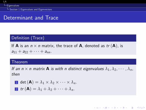
De�nition (Trace)

If A is an n� n matrix, the trace of A, denoted as tr (A), isa11 + a22 + � � �+ ann.

Theorem

If an n� n matrix A is with n distinct eigenvalues λ1,λ2, � � � ,λn,then

1 det (A) = λ1 � λ2 � � � � � λn.

2 tr (A) = λ1 + λ2 + � � �+ λn.

LA

Eigenvalues


Proof.


��a11 � λ a12 � � � a1na21 a22 � λ � � � a21...

.... . .

...an1 an2 � � � ann � λ

��= (a11 � λ) det (M11) +

n

∑i=2ai1 (�1)i+1 det (Mi1)

= (�1)n (λ� λ1) (λ� λ2) � � � (λ� λn) .

LA

Eigenvalues


Similar Matrices

Theorem

Let A and B be n� n matrices. If B is similar to A, then the twomatrices both have the same characteristic polynomial andconsequently both have the same eigenvalues.

Proof.

It is easy to verify.

pB (λ) = det (B� λI)= det

�S�1AS� λI

�= det

�S�1 (A� λI)S

�= det

�S�1

�det (A� λI) det (S)

= det (A� λI)= pA (λ) .

LA

Eigenvalues

Section 2 Systems of Linear Di¤erential Equations

Section 2 Systems of Linear Di¤erentialEquations

NOT COVERED IN THIS CLASS

LA

Eigenvalues

Section 3 Diagonalization


LA

Eigenvalues


Diagonalization

De�nition

An n� n matrix A is said to be diagonalizable if there exist anonsigular matrix X and a diagonal matrix D such thatX�1AX = D. We say that X diagonalized A.

Theorem

An n� n matrix A is diagonalizable if and only if A has n linearlyindependent eigenvectors.

LA

Eigenvalues


Example

Assume A =

24 3 �1 �22 0 �22 �1 �1

35. We havepA (λ) = det (A� λI) = �λ (λ� 1)2.For λ1 = 0, we have a eigenvector (1, 1, 2)

T .For λ2 = 1, we have eigenvectors (1, 2, 0)

T and (1, 0, 1)T .

Let X =

24 1 1 11 2 01 0 1

35. We have X�1 =24 �2 1 2

1 0 �12 �1 �1

35 andD = X�1AX.

LA

Eigenvalues


Defective Matrices

De�nition

An n� n matrix A has fewer than n linearly independenteigenvectors, we say that A is defective. An defective matrix is notdiagonalizable.

Examples

A =

24 2 0 00 4 01 0 2

35 and B =24 2 0 0�1 4 0�3 6 2

35.

LA

Eigenvalues


Polynomials of Matrices

If p (x) = amxm + am�1xm�1 + � � �+ a0 is a m-degreepolynomial and A is an n� n matrix, then

p (A) = amAm + am�1Am�1 + . . .+ a0I.

If A is diagonalizable by X, i.e. D = X�1AX or A = XDX�1,then

p (A) = amAm + am�1Am�1 + . . .+ a0I= X(amDm + am�1Dm�1 + . . .+ a0I)X�1

= Xp (D)X�1.

LA

Eigenvalues


Polynomials of Matrices (Cont.)

In addition, if D =

26664λ1 0 � � � 00 λ2 � � � 0...

.... . .

...0 0 � � � λn

37775, then

p (D) =

26664p (λ1) 0 � � � 00 p (λ2) � � � 0...

.... . .

...0 0 � � � p (λn)

37775.

LA

Eigenvalues


Example

Assume p (x) = x2 + 3x � 2. Compute p (A) for

A =��2 �61 3

�.

LA

Eigenvalues


Solution

The eigenvectors are x1 = (�2, 1)T for λ1 = 1 and x2 = (�3, 1)T

for λ2 = 0. Let X =��2 �31 1

�. Then,

A = XDX�1 =��2 �31 1

� �1 00 0

� �1 31 1

�,

and

p (A) = Xp (D)X�1 =��2 �31 1

� �p (1) 00 p (0)

� �1 31 1

�=

��2 �31 1

� �2 00 �2

� �1 31 1

�=

�2 �60 4

�.

LA

Eigenvalues


Exponentials of Matrices

According to Taylor�s series, we have

ex = 1+ x +12!x2 + � � � .

For any n� n matrix A , eA is given by

eA = I+A+12!A2 + � � � .

If A is diagonalizable by X, i.e. D = X�1AX or A = XDX�1,then eA = XeDX�1.

LA

Eigenvalues


Exponentials of Matrices (Cont.)

In addition, if D =

26664λ1 0 � � � 00 λ2 � � � 0...

.... . .

...0 0 � � � λn

37775, then

eD =

26664eλ1 0 � � � 00 eλ2 � � � 0...

.... . .

...0 0 � � � eλn

37775.

LA

Eigenvalues


Example

Compute eA for A =��2 �61 3

�.

Solution

The eigenvectors are x1 = (�2, 1)T for λ1 = 1 and x2 = (�3, 1)T

for λ2 = 0. Let X =��2 �31 1

�. Then,

eA =

��2 �31 1

� �e1 00 e0

� �1 31 1

�=

�3� 2e 6� 6ee � 1 3e � 2

�.

LA

Eigenvalues


Markov Chains

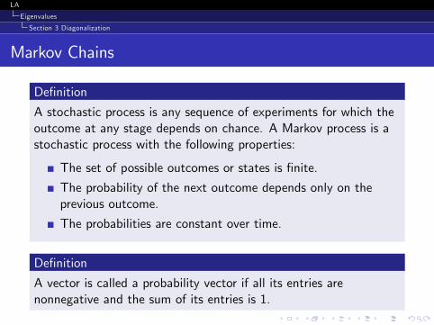
De�nition

A stochastic process is any sequence of experiments for which theoutcome at any stage depends on chance. A Markov process is astochastic process with the following properties:

The set of possible outcomes or states is �nite.

The probability of the next outcome depends only on theprevious outcome.

The probabilities are constant over time.

De�nition

A vector is called a probability vector if all its entries arenonnegative and the sum of its entries is 1.

LA

Eigenvalues


Blue-Green Color Blindness (Sex-Linked Genes)

Let x (i )1 be the proportion of genes for color blindness in the male

population, and x (i )2 be the proportion of genes for color blindnessin the female population. Then,(

x (1)1 = x (0)2x (1)2 = 1

2x(0)1 + 1

2x(0)2

=)�0 112

12

� "x (0)1x (0)2

#=

"x (1)1x (1)2

#.

Let A =�0 112

12

�. We have

A =�1 �21 1

� �1 00 � 1

2

� � 13

23

� 13

13

�.

LA

Eigenvalues


(Cont.)

limn!∞

x(n) = limn!∞

Anx(0)

= limn!∞

�1 �21 1

� �1 00 � 1

2

�n � 13

23

� 13

13

�x(0)

= limn!∞

�1 �21 1

� �1n 00

�� 12

�n �n � 13

23

� 13

13

�x(0)

=

24 x (0)1 +2x (0)23

x (0)1 +2x (0)23

35 .

LA

Eigenvalues


Theorems of Markov Chains

Theorem

If a Markov chain with an n� n transition matrix A converges to asteady-state vector x, then

1 x is a probability vector.2 λ1 = 1 is an eigenvalue of A and x is an eigenvectorbelonging to λ1 = 1.

Theorem

If λ1 = 1 is a dominant eigenvalue1 of a stochastic matrix A, thenthe Markov chain with transition A will converge to a steady-statevector.

1An eigenvalue λ of a matrix A is called a dominant eigenvalue if��λ0�� < jλj

for all other eigenvalues λ0 of A.

LA

Eigenvalues

Section 4 Hermitian Matrices


LA

Eigenvalues


Complex Inner Products

De�nition

Let V be a vector space over the complex numbers. An innerproduct on V is an operation that assigns to each pair of vectors zand w in V a complex number hz,wi satisfying the followingconditions.

hz, zi � 0. hz, zi = 0 if and only if z = 0.hz,wi = hw, zi for all z and w in V.hαz+ βw,ui = α hz,ui+ β hw,ui.

Problem

Prove that hu, αz+ βwi = α hu, zi+ β hu,wi.

LA

Eigenvalues


Lengths of Complex Numbers and Complex Vectors

If α = a+ bi is a complex scalar, the length of α is given by

jαj =p

αα =pa2 + b2.

If z = (z1, z2, . . . , zn)T is a vector in Cn, the length of z is

given by

kzk =�jz1j2 + jz2j2 + � � �+ jzn j2

�1/2

= (z1z1 + z2z2 + � � �+ znzn)1/2

=�zT z

�1/2

Let zH = zT . Then, kzk =�zHz

�1/2.

LA

Eigenvalues


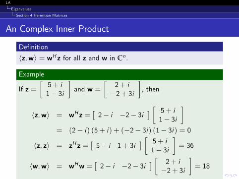
An Complex Inner Product

De�nition

hz,wi = wHz for all z and w in Cn.

Example

If z =�5+ i1� 3i

�and w =

�2+ i�2+ 3i

�, then

hz,wi = wHz =�2� i �2� 3i

� � 5+ i1� 3i

�= (2� i) (5+ i) + (�2� 3i) (1� 3i) = 0

hz, zi = zHz =�5� i 1+ 3i

� � 5+ i1� 3i

�= 36

hw,wi = wHw =�2� i �2� 3i

� � 2+ i�2+ 3i

�= 18

LA

Eigenvalues


Conjugate and Hermitian

De�nition

M is a m� n matrix with mij = aij + ibij for each i and j . IfA = (aij ) and B = (bij ), then

M = A+ iB.The conjugate of M, denoted by M, is A� iB.MH is the transport of M.

Theorem

If A,B 2 Cm�n and C 2 Cn�r , then�AH�H= A.

(αA+ βB)H = αAH + βBH .

(AC)H = CHAH .

LA

Eigenvalues


Hermitian Matrices

De�nition

A matrix M is said to be Hermitian if M =MH .

Example

M =

�3 2� i

2+ i 4

�.

Theorem

The eigenvalues of a Hermitian matrix are all real. Furthermore,eigenvectors belonging to distinct eigenvalues are orthogonal.

LA

Eigenvalues


Proof.

Let A be a Hermitian matrix, λ be an eigenvalue of A, and x bean eigenvectors belonging to λ.

Let α = xHAx. α is real sinceα = αH =

�xHAx

�H= xHAx = α.

In addition, since we have α = xHAx = xHλx = λ kxk2, wehave λ = α

kxk2 is real.

If x1 and x2 are eigenvectors belonging to distinct eigenvalues λ1and λ2,respectively.

(Ax1)H x2 = xH1 A

Hx2 = xH1 Ax2 = λ2xH1 x2.

(Ax1)H x2 =

�xH2 Ax1

�H=�λ1xH2 x1

�H= λ1xH1 x2.

It follows that hx2, x1i = xH1 x2 = 0.

LA

Eigenvalues


Unitary

De�nition

An n� n matrix U is said to be unitary if its column vectors forman orthonormal set in Cn, i.e. UHU = I and U�1 = UH .

PS. A real unitary matrix is an orthogonal matrix.

Corollary

If the eigenvalues of a Hermitian matrix A are distrinct, then thereexists a unitary matrix U that diagonalizes A.

LA

Eigenvalues


Example

Assume A =�

2 1� i1+ i 1

�. Then,

pA (λ) =

�� 2� λ 1� i1+ i 1� λ

�� = λ (λ� 3).

λ1 = 3) x1 =�1� i1

�; λ2 = 0) x2 =

��11+ i

�.

u1 = 1kx1k =

1p3

�1� i1

�; u2 = 1

kx2k =1p3

��11+ i

�.

Let U = 1p3

�1� i �11 1+ i

�. Then,

UHAU =1p3

�1+ i 1�1 1� i

� �2 1� i

1+ i 1

� �1� i �11 1+ i

�=

�3 00 0

�.

LA

Eigenvalues


Schur�s Theorem

Theorem

For each n� n matrix A, there exists a unitary matrix U such thatUHAU is upper triangular.

The factorization A = UTUH is referred to as the Schurdecomposition of A.If A is Hermitian, the matrix T will be diagonal. (SpectralTheorem)

LA

Eigenvalues


Proof of Schur�s Theorem

Proof.

This theorem can be proved by induction on n.If n = 1, obviously the result is correct.Assume the hypothesis holds for k � k matrices, and let A be a(k + 1)� (k + 1) matrix.

Let λ1 be an eigenvalue of A, and let w1 be a uniteigenvector belonging to λ1. Using the Gram-Schmidtprocess, construct an orthonormal basis fw1,w2, � � � ,wk+1g.

WHAW is a matrix of the form

26664λ1 � � � � �0... Mk�k0

37775.

LA

Eigenvalues


(Cont.)

Since M is a k � k matrix, there exist a k � k unitary matrix V1such that VH1 MV1 = T1, where T1 is triangular. Let

V =

266641 0 � � � 00... V10

37775 .Here V is unitary and

VHWHAWV

=

26664λ1 � � � � �0... VH1 MV10

37775 =26664

λ1 � � � � �0... T10

37775 = T.

LA

Eigenvalues


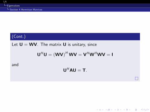
(Cont.)

Let U =WV. The matrix U is unitary, since

UHU = (WV)HWV = VHWHWV = I

andUHAU = T.

LA

Eigenvalues


Example

Let A =

24 4625 �1 28

250 3 0325 2 29

25

35. Find the Schur decomposition of A.Solution

First, �nd an eigenvalue and an eigenvector for the eigenvalue.

pA (λ) = det (A� λI)

= det

0@24 4625 � λ �1 28

250 3� λ 0325 2 29

25 � λ

351A= �λ3 + 6λ2 � 11λ+ 6

= � (λ� 1) (λ� 2) (λ� 3) .

LA

Eigenvalues


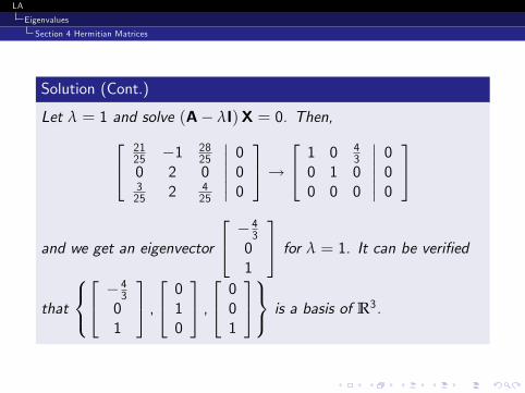
Solution (Cont.)

Let λ = 1 and solve (A� λI)X = 0. Then,24 2125 �1 28

250 2 0325 2 4

25

��000

35!24 1 0 4

30 1 00 0 0

��000

35

and we get an eigenvector

24 � 4301

35 for λ = 1. It can be veri�ed

that

8<:24 � 4

301

35 ,24 010

35 ,24 001

359=; is a basis of R3.

LA

Eigenvalues


Solution (Cont.)

Applying Gram-Schmidt process, we have w1 =

24 � 45035

35,w2 =

24 010

35, and w3 =24 3

5045

35. Let W =

24 � 45 0 3

50 1 035 0 4

5

35. Then,

WHAW =

24 � 45 0 3

50 1 035 0 4

5

35H 24 4625 �1 28

250 3 0325 2 29

25

3524 � 45 0 3

50 1 035 0 4

5

35=

24 1 2 �10 3 00 1 2

35 .

LA

Eigenvalues


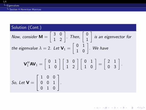
Solution (Cont.)

Now, consider M =

�3 01 2

�. Then,

�01

�is an eigenvector for

the eigenvalue λ = 2. Let V1 =�0 11 0

�. We have

VH1 AV1 =�0 11 0

� �3 01 2

� �0 11 0

�=

�2 10 3

�.

So, Let V =

24 1 0 00 0 10 1 0

35.

LA

Eigenvalues


Solution (Cont.)

We have

VH�WHAW

�V =

24 1 0 00 0 10 1 0

3524 1 2 �10 3 00 1 2

3524 1 0 00 0 10 1 0

35=

24 1 �1 20 2 10 0 3

35 .Let

U =WV =

24 � 45 0 3

50 1 035 0 4

5

3524 1 0 00 0 10 1 0

35 =24 � 4

535 0

0 0 135

45 0

35 .

LA

Eigenvalues


Solution (Cont.)

We have

UHAU =

24 � 45 0 3

535 0 4

50 1 0

3524 4625 �1 28

250 3 0325 2 29

25

3524 � 45

35 0

0 0 135

45 0

35=

24 1 �1 20 2 10 0 3

35and

A =

24 � 45

35 0

0 0 135

45 0

3524 1 �1 20 2 10 0 3

3524 � 45 0 3

535 0 4

50 1 0

35 .

LA

Eigenvalues


Spectral Theorem

Theorem

If A is Hermitian, then there exists a unitary matrix U thatdiagonalizes A.

Proof.

There is a unitary matrix U such that T = UHAU, where T isupper triangular. TH = (UHAU)H = UHAHU = UHAU = T.Therefore, T is Hermitian and diagonal.

Corollary

If A is a real symmetric matrix, then there exists an orthogonalmatrix U that diagonalizes A.

LA

Eigenvalues


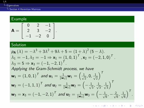
Example

A =

24 0 2 �12 3 �2�1 �2 0

35.Solution

pA (λ) = �λ3 + 3λ2 + 9λ+ 5 = (1+ λ)2 (5� λ).λ1 = �1,λ2 = �1) x1 = (1, 0, 1)

T , x2 = (�2, 1, 0)T .λ3 = 5) x3 = (�1,�2, 1)T .Applying the Gram-Schmidt process, we have

w1 = (1, 0, 1)T and u1 = 1

kw1kw1 =�1p2, 0, 1p

2

�Tw2 = (�1, 1, 1)T and u2 = 1

kw2kw2 =�� 1p

3, 1p

3, 1p

3

�Tw3 = x3 = (�1,�2, 1)T and u2 = 1

kw3kw3 =�� 1p

6,� 2p

6, 1p

6

�T.

LA

Eigenvalues


Solution (Cont.)

Let U =

2641p2� 1p

3� 1p

60 1p

3� 2p

61p2

1p3

1p6

375.Then, UHAU =

24 �1 0 00 �1 00 0 5

35.

LA

Eigenvalues


Normal Matrices

Some non-Hermitian matrices possess complete orthonormalsets of eigenvectors.

e.g. skew symmetric and skew Hermitian matrices. (A is skewHermitian if AH = �A).

If A is a matrix with a complete orthonormal set ofeigenvectors, A = UDUH , where U is unitary and D is adiagonal matrix.

In general, DH 6= D.AAH = AHA.

AAH = UDUHUDHUH = UDDHUH .AHA = UDHUHUDUH = UDDHUH .

LA

Eigenvalues


Normal Matrices

De�nition

A matrix A is said to be normal if AAH = AHA.

Theorem

A matrix A is normal if and only if A possesses a completeorthonormal set of eigenvectors.

LA

Eigenvalues


Proof.

There exists a unitary matrix U and a triangular matrix T suchthat T = UHAU.We have TTH = UHAAHU and THT = UHAHAU. SinceAAH = AHA, T is also normal.Comparing the diagonal elements of TTH and THT, we have

jt11j2 + jt12j2 + � � �+ jt1n j2 = jt11j2

jt22j2 + � � �+ jt2n j2 = jt12j2 + jt22j2...

jtnn j2 = jt1n j2 + jt2n j2 + � � �+ jtnn j2

It follows that tij = 0 whenever i 6= j . Thus, U diagonalize A andthe column vectors of U are eigenvectors of A.

LA

Eigenvalues

Section 5 The Singular Value Decomposition


LA

Eigenvalues


SUV Decomposition

A = UΣVT

A: an m� n matrix. (Assume m � n.)U: an m�m orthogonal matrix.

V: an n� n orthogonal matrix.

Σ =

266666664

σ1 0 0 0

0 σ2 0...

0 0. . . 0

...... σn

0 0 � � �

377777775: an m� n matrix whose o¤

diagonal entries are all 0�s and whose diagonal elementssatisfy σ1 � σ2 � � � � � σn � 0.

LA

Eigenvalues


The SVD Theorem

Objectives

The σi�s determined by this factorization are unique and calledthe singular value decomposition.The rank of A equals the number of nonzero singular values.

Theorem

If A is an m� n matrix, then A has a singular value decomposition.

LA

Eigenvalues


Proof.

If A = UΣVT , then ATA = VΣTΣVT is diagonalized by V.

Let λ1,λ2, � � � ,λn be eigenvectors of ATA sorted indescending order, i.e. λ1 � λ2 � � � � � λn � 0, andv1, v2, � � � , vn are corresponding eigenvectors. (Actually, it istrue that ATA can be diagonalized by a unitary matrix.)We have λ1 � 0 for all i = 1, 2, � � � , n. (Hint:kAvik2 = λi kvik2.)Then, V = (v1, � � � , vn) and σi = λ1/2

i .

LA

Eigenvalues


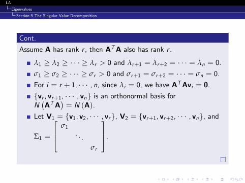
Cont.

Assume A has rank r , then ATA also has rank r .

λ1 � λ2 � � � � � λr > 0 and λr+1 = λr+2 = � � � = λn = 0.

σ1 � σ2 � � � � � σr > 0 and σr+1 = σr+2 = � � � = σn = 0.

For i = r + 1, � � � , n, since λi = 0, we have ATAvi = 0.fvr , vr+1, � � � , vng is an orthonormal basis forN�ATA

�= N (A).

Let V1 = fv1, v2, � � � , vrg, V2 = fvr+1, vr+2, � � � , vng, and

Σ1 =

264 σ1. . .

σr

375.

LA

Eigenvalues


Cont.

Assume A = UΣVT . Then, AV = UΣ.

Comparing the �rst r column of each side, we see thatAvj = σjuj for j = 1, � � � , r .Let uj = 1

jσj jAvj for j = 1, � � � , r , and U1 = (u1, � � � ,ur ).We have AV1 = U1Σ1.The column vector of U1 form an orthonormal set. (why?)

Since rank (A) = r , the column vector of U1 form anorthonormal set of R (A).

LA

Eigenvalues


Cont.

The vector space R (A)? = N�AT�has dimension m� r .

Let fur+1,ur+2, � � � ,ung be an orthonormal basis forN�AT�, and set U2 = (ur+1,ur+2, � � � ,un) and

U = (U1 U2).Then,

UΣVT = (U1 U2)�

Σ1 00 0

��VT1VT2

�= U1Σ1VT1 = AV1V

T1 = A.

LA

Eigenvalues


Observations

The singular value σ1, σ2, � � � , σn of A are unique; however,the matrices U and V are not unique.Since V diagonalizes ATA, vj�s are eigenvectors of ATA.Since AAT = UΣΣTU, it follows that U diagonalizes AAT

and that the uj�s are eigenvectors of AAT .Comparing the jth columns of each side of the equationAV = UΣ, we get Avj = σjuj for j = 1, � � � , n. Similarly,from ATU = VΣT , we have Auj = σjvj for j = 1, � � � , n andAT uj = 0 for j = n+ 1, � � � ,m.

The vj�s are called the right singular vectors of A.The uj�s are called the left singular vectors of A.

LA

Eigenvalues


Observations (cont.)

If A has rank r , then

v1, v2, � � � , vr form an orthonormal basis for R�AT�.

vr+1, vr+2, � � � , vn form an orthonormal basis for N (A).u1, � � � ,ur form an orthonormal basis for R (A).ur+1,ur+2, � � � ,un form an orthonormal basis for N

�AT�.

The rank of the matrix A is equal to the number of itsnonzero singular values (where singular values are countedaccording to multiplicity).

In the case that A has rank r < n, if we setU1 = (u1, � � � ,ur ),V1 = fv1, v2, � � � , vrg, and Σ1 as inequation (1), then A = U1Σ1VT1 . The factorization is calledthe compact form of the SVD of A.

LA

Eigenvalues


Example

Compute the SVD of A =

24 1 11 10 0

35.Solution

First, ATA =�2 22 2

�has an eigenvector (1, 1)T for eigenvalue

λ1 = 4, and an eigenvector (1,�1)T for eigenvalue λ2 = 0. So thesingular values of A are σ1 =

p4 = 2 and σ2 = 0. So, the singular

values of A are σ1 = 2 and σ2 = 0, and V = 1p2

�1 11 �1

�.

LA

Eigenvalues


Solution ((Cont.))

From observation 4,

u1 =1

σ1Av1 =

12

24 1 11 10 0

35 " 1p21p2

#=

2641p21p20

375 .The remaining column vectors of U must from an orthonormalbasis for N

�AT�.nw2 = (1,�1, 0)T ,w3 = (0, 0, 1)T

ois a basis of N

�AT�.

LA

Eigenvalues


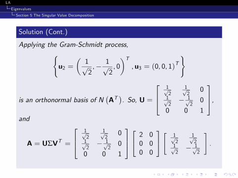
Solution (Cont.)

Applying the Gram-Schmidt process,(u2 =

�1p2,� 1p

2, 0�T

,u3 = (0, 0, 1)T

)

is an orthonormal basis of N�AT�. So, U =

2641p2

1p2

01p2� 1p

20

0 0 1

375,and

A = UΣVT =

2641p2

1p2

01p2� 1p

20

0 0 1

37524 2 00 00 0

35 " 1p2

1p2

1p2� 1p

2

#.

LA

Eigenvalues


The Closest Matrix

If A is an m� n matrix of rank r and 0 < k < r , we wouldlike to �nd a matrix in Rm�n of rank k that is closest to Aw.r.t. the Frobenius norm.

In other words, letM be the set of all m� n matrices of rankk or less. I would like to �nd a matrix X inM such that

kA�XkF = minS2M

kA� SkF .

Lemma

If A is an m� n matrix and Q is an m�m orthogormal matrix,then

kQAkF = kAkF .

LA

Eigenvalues


Theorem

Let A = UΣVT be an m� n matrix, and letM denote the set ofall m� n matrices of rank k or less, where 0 < k < rank (A). If Xis a matrix inM satisfying kA�XkF = minS2M kA� SkF , then

kA�XkF =�σ2k+1 + σ2k+2 + � � �+ σ2r

�1/2.

In particular, if A0= UΣ0VT , where

Σ0 =

26664σ1

. . . 0σk

0 0

37775 =�

Σk 00 0

�

then A�A0 F = �σ2k+1 + σ2k+2 + � � �+ σ2r�1/2

= minS2M

kA� SkF .

LA

Eigenvalues

Section 6 Quadratic Forms


LA

Eigenvalues


LA

Eigenvalues


LA

Eigenvalues


LA

Eigenvalues


LA

Eigenvalues


LA

Eigenvalues


LA

Eigenvalues


LA

Eigenvalues


LA

Eigenvalues


LA

Eigenvalues


LA

Eigenvalues

Section 7 Positive De�nite Matrices


LA

Eigenvalues


LA

Eigenvalues


LA

Eigenvalues


LA

Eigenvalues


LA

Eigenvalues


LA

Eigenvalues


LA

Eigenvalues

Section 8 Nonnegative Matrices

Section 8 Nonnegative Matrices

NOT COVERED IN THIS CLASS

Date post:	29-Mar-2020
Category:	Documents
Upload:	others
View:	20 times
Download:	3 times

Linear Algebrayi/Courses/LinearAlgebra...LA Eigenvalues Section 1 Eigenvalues and Eigenvectors How...

Documents