Linear and Nonlinear Analysis of High Dynamic Impact ... · PDF fileLinear and Nonlinear...

Linear and Nonlinear Analysis of High Dynamic Impact Events with Creo Simulate and Abaqus/Explicit

SAXSIM 2015, TU Chemnitz

Rev. 1.1 | 31.03.2015

Dr.-Ing. Roland Jakel

At a glance: Altran, a global leader

€ 1,756m

2014 Revenues

AMERICA

EUROPE

ASIA

23,000+

Innovation Makers

5

Industries

20+

Countries

2

Our Customers

3

AUTOMOTIVE, INFRASTRUCTURE

& TRANSPORTATION

AEROSPACE,

DEFENCE & RAILWAYS

ENERGY, INDUSTRY

& LIFE SCIENCES

FINANCIAL SERVICES

& PUBLIC SECTOR

TELECOMS & MEDIA

Rev. 1.1 | 31.03.2015

1. Description of the Example Problem

2. Analysis of the Problem in Creo Simulate 2.1 Solution method coded in Creo Simulate 2.2 Model setup 2.3 Modal analysis 2.4 Dynamic time analysis with impulse function applied 2.5 Dynamic time analysis with half sine wave applied 2.6 Conclusions

3. Solution of the Problem in Abaqus/Explicit 3.1 The explicit solver for dynamic analysis 3.2 Framework for modeling damage and failure in Abaqus 3.3 Damage initiation criteria for ductile materials 3.4 Damage evolution 3.5 Definition of the ideal material response curve 3.6 Iterative procedure for defining a rough material response curve with only very limited tensile test data available 3.7 Transfer to the example problem

4. References

4

Table of Contents

Slide:

5

6-15 6

8

9

11

13

15

16-31 16 17 18 20 21 24

29

32

Rev. 1.1 | 31.03.2015

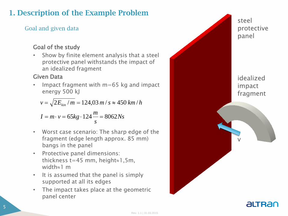
Goal and given data

Goal of the study

• Show by finite element analysis that a steel protective panel withstands the impact of an idealized fragment

Given Data

• Impact fragment with m=65 kg and impact energy 500 kJ

• Worst case scenario: The sharp edge of the fragment (edge length approx. 85 mm) bangs in the panel

• Protective panel dimensions: thickness t=45 mm, height1,5m, width1 m

• It is assumed that the panel is simply supported at all its edges

• The impact takes place at the geometric panel center

5

1. Description of the Example Problem steel protective panel

idealized impact fragment

v

Nss

mkgvmI

hkmsmmEv kin

806212465

/450/03,124/2

Rev. 1.1 | 31.03.2015

2.1 Solution method coded in Creo Simulate

Basic Equation for Dynamic Systems

• Creo Simulate can only solve for dynamic problems which can be described with the following linear differential equation of second order:

• Herein, we have [M]=mass matrix, [C]=damping matrix, [K]=stiffness matrix, {F}=force vector, {u}=displacement vector and its derivatives

Solution Sequence:

• Before a dynamic analysis is performed in Simulate, a damping-free modal analysis, , is carried out to obtain the modal base for the modal transformation

• The system is then transformed from physical to modal space by replacing the physical coordinates

• Herein, is the eigenvector matrix, and modal coordinates; has a number of rows equal to the DOF in the model, and columns equal to the number of modes; has one column and rows equal to the number of modes

• In a subsequent dynamic analysis, in which modal damping C=2M and a forcing function is added, we have M, C and K as diagonal matrices now in modal coordinates

• After the solution is performed, the solution is transformed back into physical space for post-processing

Remark: This solution method is used in many FEM codes for linear, small damped dynamic systems because of its computational efficiency!

6

2. Analysis of the Problem in Creo Simulate

0 uKuM

u

)(tFuKuCuM

Rev. 1.1 | 31.03.2015

2.1 Solution method coded in Creo Simulate

Limitations of the solution method

• We have only a linear system (all matrices are constant), that means no nonlinearities can be taken into account like

contact

change of constraints (boundary conditions)

nonlinear material

• Only modal damping can be applied (max. 50 % of critical damping, =1) to keep the damping matrix diagonal and therefore run times short

Special challenge when solving the described problem

• Contact between panel and idealized fragment cannot be modelled, therefore the unknown impact force-vs-time curve cannot be computed

• The impact force must therefore be applied as external force, using some assumptions

• Most conservative approach is to model the impact as impulse function (Dirac impulse), that means the impulse of 8062 Ns is applied in an infinite short time span

• Later, conservatism may be removed by assuming the force-vs.-time curve to be a half sine function

7


Rev. 1.1 | 31.03.2015

2.2 Model setup

• Plate is meshed with p-bricks (mapped mesh)

• To “reduce” the singularity of the edge constraint (simple support), an Isolate for Exclusion AutoGEM Control (IEAC) is used (exclusion of stresses > p-level of 3)

• Linear steel material applied with yield limit 405 MPa

• We analyze the failure index for the distortion energy criterion

8


Rev. 1.1 | 31.03.2015

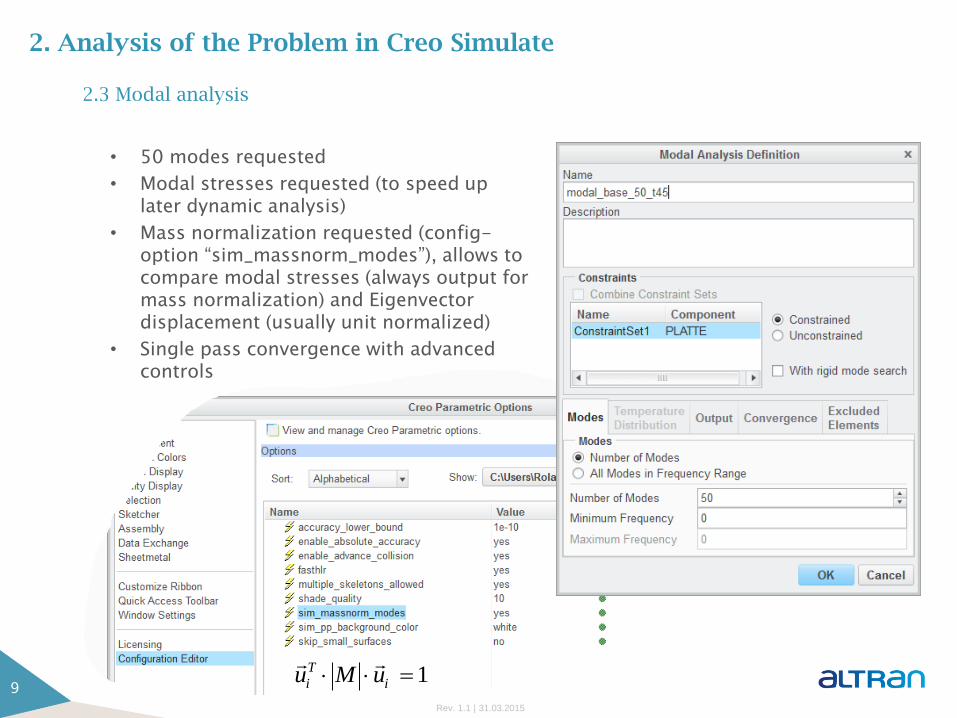
2.3 Modal analysis

• 50 modes requested

• Modal stresses requested (to speed up later dynamic analysis)

• Mass normalization requested (config-option “sim_massnorm_modes”), allows to compare modal stresses (always output for mass normalization) and Eigenvector displacement (usually unit normalized)

• Single pass convergence with advanced controls

9


1 i

T

i uMu

Rev. 1.1 | 31.03.2015

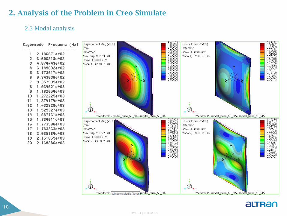
2.3 Modal analysis

10


Rev. 1.1 | 31.03.2015

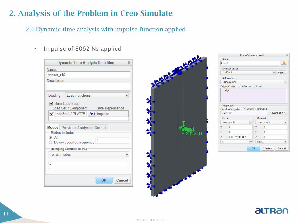
2.4 Dynamic time analysis with impulse function applied

• Impulse of 8062 Ns applied

11


Rev. 1.1 | 31.03.2015

2.4 Dynamic time analysis with impulse function applied

• Time step t=0,1 ms with max. failure index (in scale)

12


• Movie of impact event (in scale, duration 1 ms)

Rev. 1.1 | 31.03.2015

2.5 Dynamic time analysis with half sine wave applied

• Results show max. von Mises stress >50 times higher than yield limit at time t=0,1 ms

• Approach is much too conservative, need to remove conservatism by assuming the impact is in form of a half sine wave with duration TI=T/2 of the first fundamental plate Eigenfrequency f0

• The force-vs-time curve of the half sine impact can be described as follows:

• The impulse then becomes:

• This has been coded into the Simulate form sheet for dynamic time analysis, see right

13


)sin()( max tFtF

NfII

F

dttFIIT

t

6

00

max

0max

10538,52

)sin(

Rev. 1.1 | 31.03.2015

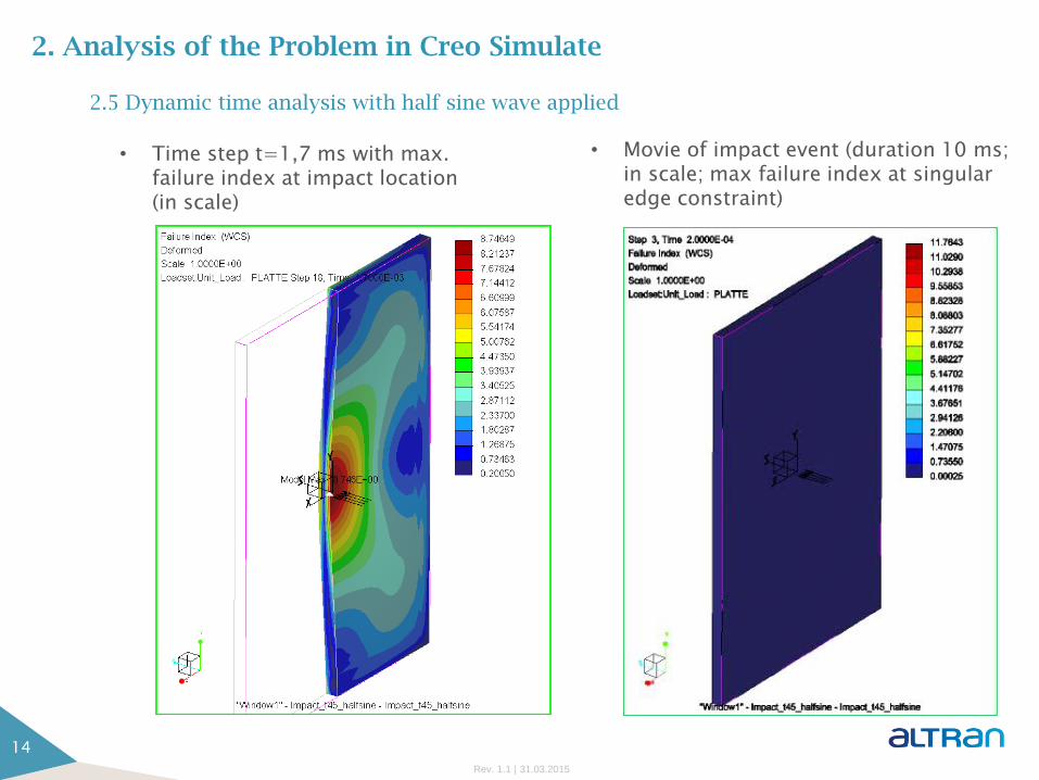
2.5 Dynamic time analysis with half sine wave applied

• Time step t=1,7 ms with max. failure index at impact location (in scale)

14


• Movie of impact event (duration 10 ms; in scale; max failure index at singular edge constraint)

Rev. 1.1 | 31.03.2015

2.6 Conclusions

• With the less conservative approach, max. loading at the impact location is still factor 8.7 above yield

• With the computational approach provided in Creo Simulate therefore no strength proof is possible

• The plate had to be thickened significantly in order not to leave the linear domain of validity

• Anyway, the foreseen steel has a large ductile region that could take significant kinetic energy of the fragment – we need a computational approach that can take this into account

15


engineering strain [%]

engin

eeri

ng s

tress [

MPa]

Rev. 1.1 | 31.03.2015

3.1 The explicit solver for dynamic analysis

• The explicit dynamics analysis procedure in Abaqus/Explicit is based upon the implementation of an explicit integration rule together with the use of diagonal or “lumped” element mass matrices for computational efficiency [1]

• The explicit dynamic procedure requires no iterations and no tangent stiffness matrix: Herein, {Rint}, {Rext} are the internal and external load vectors; i: time increment

• The equations of motion for the body are integrated using the explicit central difference integration rule with u=displacement DOF with derivatives, respectively, and superscripts (i) increment number; (i-1/2), (i+1/2) midincrement values

• The central difference integration operator is explicit in that the kinematic state can be advanced using known values from the previous increment

• The stability limit for each integration time step is given by where max is the highest element frequency in the model

• An analysis typically has some 100,000 increments

16

3. Solution of the Problem in Abaqus/Explicit

)2

1(

)1()()1(

)()()1(

)2

1()

2

1(

2

iiii

iii

ii

utuu

utt

uu

max/2 t

iext

iii RRuCuM int

Rev. 1.1 | 31.03.2015

3.2 Framework for modeling damage and failure in Abaqus

To specify the material failure in Abaqus, four distinct steps are necessary:

1. The definition of the effective (or undamaged) material response (points a-b-c-d‘)

2. A damage initiation criterion (c)

3. A damage evolution law (c-d)

4. A choice of element deletion whereby elements can be removed from the calculations once the material stiffness is fully degraded (d)

Note: D is the overall damage variable (D=0…1). After damage initiation, the stress tensor in the material is given by the scalar damage equation with =stress in the material with absence of damage

17


Note: Image shows true stress vs. log strain, the curve should not be mixed up with a classical tensile test

diagram (engineering stress vs. engineering strain)!

a

b

c

d

d'

(D=1)

)1( D

Rev. 1.1 | 31.03.2015

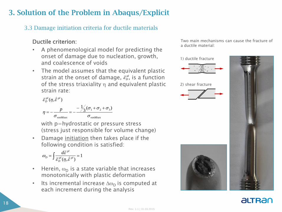
3.3 Damage initiation criteria for ductile materials

Ductile criterion:

• A phenomenological model for predicting the onset of damage due to nucleation, growth, and coalescence of voids

• The model assumes that the equivalent plastic strain at the onset of damage, , is a function of the stress triaxiality and equivalent plastic strain rate: with p=hydrostatic or pressure stress (stress just responsible for volume change)

• Damage initiation then takes place if the following condition is satisfied:

• Herein, D is a state variable that increases monotonically with plastic deformation

• Its incremental increase D is computed at each increment during the analysis

18


1) ductile fracture

2) shear fracture

Two main mechanisms can cause the fracture of a ductile material:

vonMisesvonMises

plpl

D

p

)(3

1

),(

321

1),( plpl

D

pl

D

d

pl

D

Rev. 1.1 | 31.03.2015

3.3 Damage initiation criteria for ductile materials

Shear criterion:

• A phenomenological model for predicting the onset of damage due to shear band localization

• The model assumes that the equivalent plastic strain at the onset of damage, , is a function of the shear stress ratio S and equivalent plastic strain rate:

• Herein, kS is a material parameter (for example 0,3 typically for Aluminum)

• Damage initiation then takes place if the following condition is satisfied:

• Herein, S is a state variable that increases monotonically with plastic deformation

• Its incremental increase S is computed at each increment during the analysis

Local necking:

• This is an instability problem which is computed automatically in nonlinear elastoplastic analysis if volume elements are used

• Just if shell elements are used, special damage initiation criteria for sheet metal instability have to be defined

19


local necking (instability)

max/)(

),(

pkSvonMisesS

pl

S

pl

S

1),( pl

S

pl

S

pl

S

d

pl

S

Rev. 1.1 | 31.03.2015

3.4 Damage evolution

The damage evolution capability for ductile metals

• assumes that damage is characterized by the progressive degradation of the material stiffness, leading to material failure;

• uses mesh-independent measures (either plastic displacement upl or physical energy dissipation) to drive the evolution of damage after damage initiation;

• takes into account the combined effect of different damage mechanisms acting simultaneously on the same material and includes options to specify how each mechanism contributes to the overall material degradation; and

• offers options for what occurs upon failure, including the removal of elements from the mesh.

20


Rev. 1.1 | 31.03.2015

3.5 Definition of the ideal material response curve

Intuitively we may think a simple tensile test is sufficient, but…

• The classical uniaxial tensile test is not well suited to measure the ideal material response of ductile materials, since it shows necking, a superimposed instability problem

• The data can therefore just be used until the maximum value of the engineering stress vs. engineering strain curve is reached

• Refined test methods, for example in [4], or other specimen types [5] must be used to obtain reliable data

What happens during a uniaxial tensile test of a ductile specimen [3]?

• Until the maximum value of the engineering stress/strain-curve is reached, the stress state is uniaxial

• Further elongation leads to instability (necking), what locally creates a two-dimensional stress state at the necked surface and a three-dimensional stress state within the specimen

• The uniaxial stress outside the necked region then decreases, the strain rate in the necked region increases!

• The real uniaxial fracture strain can therefore not easily be measured with this test (see [4] for a refined approach)

• A better orientation for the fracture strain out of this test may be the percentage reduction of area after fracture, Z

21


Rev. 1.1 | 31.03.2015


The uniaxial tensile test

• Fracture strain: (Lu=rupture length, L0=initial length)

• Reduction of area: (Su=smallest cross section at rupture location; S0=initial cross section)

• As longer the tensile test rod, as smaller the engineering strain until failure:

22


Engineering stress-strain curve of soft steel for different ratios of the tensile rod A=L0/d0 [2]

Ag

0

0

S

SSZ u

0

0

L

LLA u

Uniform elongation (without necking)

Non-uniform elongation with necking

Rev. 1.1 | 31.03.2015


Material Laws

• To fit test data, plasticity laws may be used from literature

• For example, Creo Simulate offers three material laws for describing plasticity: linear plasticity, power (potential) law, exponential law [3]

• The laws may be used especially to extrapolate the true stress-strain curve to higher strains, if for example just tensile test data is available

• However, Abaqus requires any tabular input for the curve (true stress vs. log. plastic strain) and interpolates between the data points

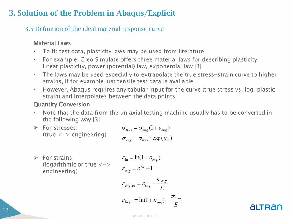
Quantity Conversion

• Note that the data from the uniaxial testing machine usually has to be converted in the following way [3]

For stresses: (true <-> engineering)

For strains: (logarithmic or true <-> engineering)

23


Rev. 1.1 | 31.03.2015

3.6 Iterative procedure for defining a rough material response curve with only very limited

tensile test data available

For the material foreseen for our example problem, just data from 5 tensile test specimens is available, so the following assumptions & simplifications where done:

• No temperature and strain rate dependency

• No stress state dependency (just values for triaxiality =1/3=pure tension entered)

• Damage initiation only according to the simple ductile criteria

• Damage evolution linear for just a small plastic fracture displacement

Then, the following steps have been performed:

1. A 2D axial symmetric FEM-model of the tensile test specimen is created in Abaqus. A small imperfection (diameter reduction) is used to have the start of necking at the specimen center and not at the constraints

2. The ideal material response curve in the region of uniform elongation is simply calculated out of the uniaxial test results (see equations on previous slide)

3. The ideal material response curve after onset of local necking is iteratively trimmed by comparing the measured force of the test (engineering stress) with the reaction force of the FEM analysis (since the analysis delivers only true stresses). Initially, damage is not taken into account in the FEM model

4. After sufficient curve fit, the damage parameter is activated (with element removal for D=1). Start value for the fracture strain is taken from Z and trimmed iteratively until the calculated curve also fits on its “right end” within the measured curve

Note: This is no recommended procedure! It shall only give listeners new to this topic an impression about the difficulties of a simple tensile test!

24


mmu pl

f 3,0

Rev. 1.1 | 31.03.2015



• Comparison of test results with FEM analysis - forces

25


Drop of all the curves (except the input curve) always comes from local necking, not from damage initiation!

Entered curve is without necking!

Here, damage initiation takes place

Rev. 1.1 | 31.03.2015



• Ideal material response curves

26


mmu pl

f

pl

D

3,0

9,0)3/1(

Response curve expressed in the required Abaqus input format

0

1

D

D0D

0D

Rev. 1.1 | 31.03.2015



• Von Mises stress within the 2D axial symmetric FEM of the tensile test specimen

27


Rev. 1.1 | 31.03.2015



• Equivalent plastic strain within the 2D axial symmetric FEM of the test specimen

28


Rev. 1.1 | 31.03.2015

3.7 Transfer to the example problem

Abaqus finite element model

• Uses half symmetry

• Eight linear elements with reduced integration over the protection panel thickness

• Thickness 45 mm, in addition for comparison models with 40 mm and 35 mm thickness

• Same material model for the protection panel as used for the test specimen

• Fragment uses steel with just simple linear behavior

• Contact with friction, friction coefficient 0,1 (conservative)

29


Rev. 1.1 | 31.03.2015


• Animation of the impact event, von Mises stress; from left to right: 45, 40 and 35 mm panel thickness

30


Rev. 1.1 | 31.03.2015


• Animation of the impact event, von Mises stress; from left to right: 45, 40 and 35 mm panel thickness

31


Rev. 1.1 | 31.03.2015

[1] Without further notice, many Abaqus related information of this presentation is taken from the Abaqus 6.12 documentation manuals (Dassault Systèmes Simulia)

[2] Domke: Werkstoffkunde und Werkstoffprüfung, 9. Auflage 1981, Girardet, Essen, ISBN 3-7736-1219-2

[3] Roland Jakel: Basics of Elasto-Plasticity in Creo Simulate, Theory and Application, Presentation at the 4th SAXSIM, 17.04.2012, Rev. 2.1

[4] Sören Ehlers, Petri Varsta: Strain and stress relation for non-linear finite element simulations, Thin-Walled Structures 47 (2009), pp. 1203-1217

[5] Antonin Prantl, Jan Ruzicka, Miroslav Spaniel, Milos Moravec, Jan Dzugan, Pavel Konopík: Identification of Ductile Damage Parameters, 2013 SIMULIA Community Conference (www.3ds.com/simulia)

A good overview about simulating ductile fracture in steel may be found in: Henning Levanger: Simulating ductile fracture in steel using the finite element method: Comparison of two models for describing local instability due to ductile fracture; thesis for the degree of master of science; Faculty of Mathematics and Natural Sciences, University of Oslo, May 2012

32

4. References

http://www.3ds.com/simulia

Dr.-Ing. Roland Jakel Senior Consultant, Structural Simulation Phone: +49 (0) 421 / 557 18 4111 Mobile: +49 (0) 173 / 889 04 19 [email protected]

Henning Maue Global aircraft engineering architect ASDR group Head of Engineering ASDR Germany Technical Unit Manager Airframe Structure Phone: +49 (0) 40 35 96 31 96 122 Mobile: +49 (0) 172 83 63 335 [email protected]

Date post:	06-Feb-2018
Category:	Documents
Upload:	phambao
View:	232 times
Download:	2 times

Linear and Nonlinear Analysis of High Dynamic Impact ... · PDF fileLinear and Nonlinear...

Documents